A PRACTICAL OPTIMUM DESIGN OF STEEL STRUCTURES WITH SCATTER SEARCH METHOD AND SAP2000

A THESIS SUBMITTED TO THE GRADUATE SCHOOL OF NATURAL AND APPLIED SCIENCES

OF MIDDLE EAST TECHNICAL UNIVERSITY

BY

AHMET ESAT KORKUT

IN PARTIAL FULFILLMENT OF THE REQUIREMENTS FOR

THE DEGREE OF MASTER OF SCIENCE IN

CIVIL ENGINEERING

FEBRUARY 2013

  

iii  

Approval of the thesis:

A PRACTICAL OPTIMUM DESIGN OF STEEL STRUCTURES WITH SCATTER SEARCH METHOD AND SAP2000 submitted by AHMET ESAT KORKUT in partial fulfillment of the requirements for the degree of Master of Science in Civil Engineering Department, Middle East Technical University by, Prof. Dr. Canan Özgen Dean, Graduate School of Natural and Applied Sciences _____________________ Prof. Dr. Ahmet Cevdet Yalçıner Head of Department, Civil Engineering _____________________ Assoc. Prof. Dr. Oğuzhan Hasançebi Supervisor, Civil Engineering Dept., METU _____________________ Examining Committee Members: Prof. Dr. Mehmet Polat SAKA Civil Engineering Dept., University of Bahrain _____________________ Assoc. Prof. Dr. Oğuzhan Hasançebi Civil Engineering Dept., METU _____________________ Assoc. Prof. Dr. Uğur Polat Civil Engineering Dept., METU _____________________ Dr. Onur Pekcan Civil Engineering Dept., METU _____________________ Dr. Cenk Tort Civil Engineer, Miteng Engineering _____________________

Date: 01.02.2013 

iv  

I hereby declare that all information in this document has been obtained and presented in accordance with academic rules and ethical conduct. I also declare that, as required by these rules and conduct, I have fully cited and referenced all material and results that are not original to this work.

Name, Last name: Ahmet Esat KORKUT Signature :

v  

ABSTRACT

A PRACTICAL OPTIMUM DESIGN OF STEEL STRUCTURES WITH SCATTER SEARCH METHOD AND SAP2000

Korkut, Ahmet Esat M.Sc., Department of Civil Engineering

Supervisor: Assoc. Prof. Dr. Oğuzhan Hasançebi

February 2013, 66 pages

In the literature, a large number of metaheuristic search techniques have been proposed up to present time and some of those have been used in structural optimization. Scatter search is one of those techniques which has proved to be effective when solving combinatorial and nonlinear optimization problems such as scheduling, routing, financial product design and other problem areas. Scatter search is an evolutionary method that uses strategies based on a composite decision rules and search diversification and intensification for generating new trial points. Broodly speaking, this thesis is concerned with the use and application of scatter search technique in structural optimization. A newly developed optimization algorithm called modified scatter search is modified which is computerized in a software called SOP2012. The software SOP2012 is integrated with well-known structural analysis software SAP2000 using application programming interface for size optimum design of steel structures. Numerical studies are carried out using a test suite consisting of five real size design examples taken from the literature. In these examples, various steel truss and frame structures are designed for minimum weight according to design limitations imposed by AISC-ASD (Allowable Stress Design Code of American Institute of Steel Construction). The results reveal that the modified scatter search technique is very effective optimization technique for truss structures, yet its performance can be assessed ordinary for frame structures.   Key Words: Scatter Search, Structural Optimization, Size Optimization, Discrete Optimization

vi  

ÖZ

ÇELİK YAPILARIN DAĞINIK ARAMA ALGORİTMASI VE SAP2000 İLE PRATİK OPTİMUM TASARIMI

Korkut, Ahmet Esat M.Sc., Department of Civil Engineering

Tez Yöneticisi: Assoc. Prof. Dr. Oğuzhan Hasançebi

Şubat 2013, 66 sayfa

Literatürde, günümüze kadar, çok sayıda metasezgisel arama teknikleri önerilmiş ve bunlardan bir kısmı yapısal optimizasyonda kullanılmıştır. Zamanlama, rotalama, finansal ürün tasarımı ve diğer problem alanları gibi kombinasyonel ve doğrusal olmayan optimizasyon problemlerini çözmek için etkili olduğu kanıtlanan dağınık arama methodu metasezgisel arama tekniklerinden birisidir. Yeni deneme noktaları oluşturmak için bileşik karar kurallarını ve arama çeşitlendirme ve yoğunlaştırmayı temel alan stratejileri kullanan dağınık arama, evrimsel bir yöntemdir. Genel olarak bu tez, dağınık arama tekniğinin yapısal optimizasyonda kullanımı ve uygulanması ile ilgilidir. SOP2012 adlı bir yazılımda bilgisayarlaştırılmış, değiştirilmiş dağınık arama denilen yeni geliştirilmiş bir optimizasyon algoritması tadil edilmiştir. SOP2012 yazılımı çelik yapıların optimum boyut tasarımı için uygulama programlama arabirimini kullanarak, tanınmış yapısal analiz yazılımı SAP2000 ile entegre edilmiştir. Sayısal çalışmalar literatürden alınan beş adet gerçek boyut tasarım örneklerinden oluşan bir test grubu kullanılarak yerine getirilmiştir. Bu örneklerde çeşitli çelik kafes ve çerçeve yapılar, AISC-ASD’nin (Amerikan Çelik Konstrüksiyon Enstitüsünün Emniyet Gerilmesi Tasarım Kuralları) dayattığı tasarım kısıtlamalarına göre asgari ağırlık için tasarlanmıştır. Sonuçlar modifiye dağınık arama tekniğinin kafes yapılar için çok etkili bir optimizasyon tekniği olduğunu ortaya koymuştur, fakat çerçeve yapılar için performans sıradan değerlendirilebilir. Anahtar Kelimeler: Dağınık Arama, Yapısal Optimizasyon, Boyut Optimizasyonu

vii  

Çok Sevgili Annem, Babam ve Eşime

viii  

ACKNOWLEDGEMENTS

The author wishes to express his sincere gratitude to his thesis supervisor, Assoc. Prof. Dr. Oğuzhan Hasançebi, for his invaluable guidance, encouragement and support throughout the course of the studies and to the examining committee for their invaluable suggestions and efforts in reviewing the thesis.

ix  

TABLE OF CONTENTS ABSTRACT ................................................................................................................................................. v ÖZ ................................................................................................................................................................. vi ACKNOWLEDGEMENTS ......................................................................................................................... viii TABLE OF CONTENTS ............................................................................................................................. ix LIST OF FIGURES ...................................................................................................................................... x LIST OF TABLES ....................................................................................................................................... xii LIST OF SYMBOLS ................................................................................................................................... xiii

CHAPTERS 1. INTRODUCTION .................................................................................................................................... 1

1.1 Structural Systems ........................................................................................................................ 1 1.2 Scatter Search Method ................................................................................................................. 2 1.3 Software Development ................................................................................................................. 2 1.4 Outline of the Thesis .................................................................................................................... 2 

2. STRUCTURAL OPTIMIZATION ......................................................................................................... 3 2.1 Introduction .................................................................................................................................... 3  2.2 Elements of Optimization .............................................................................................................. 3  2.3 Mathematical Formulation ............................................................................................................ 5 2.4 Types of the Optimization Problems............................................................................................. 5 3. PROBLEM STATEMENT ...................................................................................................................... 7 3.1 Introduction .................................................................................................................................... 7 3.2 Design Variables ............................................................................................................................ 7 3.3 Objective Function ........................................................................................................................ 7 3.4 Constraints ..................................................................................................................................... 7 3.5 Handling of Constraints ................................................................................................................. 9 4. SCATTER SEARCH METHOD ............................................................................................................. 11 4.1 Introduction .................................................................................................................................... 11 4.2 Literature Survey ........................................................................................................................... 12 4.3 Algorithm of Scatter Search Method ............................................................................................ 14 4.4 Modified Scatter Search Method .................................................................................................. 17

4.4 Sample Problem ............................................................................................................................. 20 5. SOFTWARE DEVELOPMENT WITH SCATTER SEARCH METHOD ........................................... 25 5.1 Introduction .................................................................................................................................... 25 5.2 Capabilities of the Software .......................................................................................................... 25 5.3 User Interface................................................................................................................................ 26 5.4 Creating a Design Problem .......................................................................................................... 27 6. NUMERICAL EXAMPLES .................................................................................................................... 33

6.1 Introduction .................................................................................................................................... 33 6.2 Truss Problems .............................................................................................................................. 33 6.3 Frame Problems ............................................................................................................................. 42

7. CONCLUSIONS ...................................................................................................................................... 49 7.1 Conclusion ..................................................................................................................................... 49 7.2 Final Recommendations ................................................................................................................ 50

REFERENCES ............................................................................................................................................. 51 APPENDICES

A. Details of Used SAP2000 OAPI Functions ............................................................................................ 53 B. SAP2000 Results and Final Outcomes of SOP2012 .............................................................................. 57

x  

LIST OF FIGURES FIGURES

2-1. Definition of design space (Onwubiko, 2000) ............................................................................ 4 2-2. Local and global maxima (Onwubiko, 2000) ............................................................................. 5 2-3. A sizing structural optimization problem is formulated by optimizing the cross-sectional

areas of truss members (Christensen & Klarbring, 2009) .......................................................................... 5 2-4. A shape optimization problem. Find the function n(x), describing the shape of the beam-like

structure (Christensen & Klarbring, 2009) ................................................................................................. 6 2-5. Topology optimization of a truss (Christensen & Klarbring, 2009) .......................................... 6 2-6. Two-dimensional topology optimization (Christensen & Klarbring, 2009) .............................. 6 4-1. Two dimensional reference set (Glover, et al, 2000) ................................................................. 12 4-2. Scatter Search Outline (Glover, Laguna, & Marti, 2003) .......................................................... 15 4-3. A basic design of the method (Glover, et al, 2000) .................................................................... 16 4-4. Modified and standart scatter search method template .............................................................. 17 4-5. Single-point crossover implementation ...................................................................................... 19 4-6. 2-point crossover implementation ............................................................................................... 19 4-7. Uniform crossover implementation ............................................................................................ 19 4-8. The five bar truss problem ................................................................................................... 21 5-1. The SOP2012 windows ............................................................................................................... 26 5-2. File menu ..................................................................................................................................... 26 5-3. View menu ................................................................................................................................... 26 5-4. Define menu ................................................................................................................................ 27 5-5. Optimization menu ...................................................................................................................... 27 5-6. Illustration of load cases and load combination ......................................................................... 27 5-7. Assigned load combinations and unchecked status of automatic code based load

combination option ...................................................................................................................................... 28 5-8. Design code options and deflection consideration status ........................................................... 28 5-9. Setting displacement target ......................................................................................................... 28 5-10. Member grouping notepad file with .txt extension ................................................................... 29 5-11. Main screen and quick menu ..................................................................................................... 29 5-12. Opening the target design .......................................................................................................... 30 5-13. Member grouping and material assignment .............................................................................. 30 5-14. Ready section assignment options to member groups .............................................................. 30 5-15. Pre-design with SAP2000 ......................................................................................................... 31 5-16. Scatter Search Algorithm main form including model options, latest best design screen and

optimization history information screen ..................................................................................................... 31 6-1. 3D view, top view and side view of 354-member braced truss dome (Hasançebi et al., 2009) 34 6-2. Three load cases for 354-member braced truss dome (Hasançebi et al, 2009) .......................... 35 6-3. Design history of 354 member braced truss dome ..................................................................... 36 6-4. 3D view, top view and side view of 582-member space truss (Hasançebi et al, 2009) ............. 38 6-5. Design history of 582-member tower ......................................................................................... 39 6-6. Design history of 693 bar braced vault ....................................................................................... 39 6-7. 3D view, top view, side view of 693-bar braced vault (Hasançebi, 2011) ................................ 41 6-8. 3D view, top view and side view of 132-member unbraced space steel frame (Hasançebi et

al., 2009) ..................................................................................................................................................... 43 6-9. Design history of 132-member unbraced space steel frame ....................................................... 44 6-10. 3D view, top view, side view and member grouping of 568-member unbraced space steel

frame (Hasançebi et al., 2010) .................................................................................................................... 47 6-11. Design history of 568 member unbraced space steel frame ..................................................... 48 B-1. Analysis and design section verification of 354-bar truss dome results obtained by SAP2000

auto design procedure .................................................................................................................................. 57 B-2. Analysis and design section verification of 354-bar truss dome results obtained by SOP2012

with Scatter Search ...................................................................................................................................... 57 B-3. Initial design result of 354-bar truss dome obtained by SOP2012 with Scatter Search ........... 58 B-4. Final design result of 354-bar truss dome obtained by SOP2012 with Scatter Search ............. 58

xi  

B-5. Analysis and design section verification in SAP2000 of 582-bar truss space tower results obtained by SAP2000 auto design procedure ............................................................................................. 59

B-6. Analysis and design section verification in SAP2000 of 582-bar truss space tower results obtained by SOP2012 with Scatter Search .................................................................................................. 59

B-7. Initial design result of 582-bar truss space tower obtained by SOP2012 with Scatter Search .. 60 B-8. Final design result of 582-bar truss space tower obtained by SOP2012 with Scatter Search ... 60 B-9. Analysis and design section verification in SAP2000 of 693-bar braced barrel vault results

obtained by SAP2000 auto design procedure .............................................................................................. 61 B-10. Analysis and design section verification in SAP2000 of 693-bar braced barrel vault results

obtained by SOP2012 with Scatter Search .................................................................................................. 61 B-11. Initial design result of 693-bar braced barrel vault obtained by SOP2012 with Scatter

Search ........................................................................................................................................................... 62 B-12. Final design result of 693-bar braced barrel vault obtained by SOP2012 with Scatter

Search ........................................................................................................................................................... 62 B-13. Analysis and design section verification in SAP2000 of 132-member 4 story irregular

frame results obtained by SAP2000 auto design procedure ........................................................................ 63 B-14. Analysis and design section verification in SAP2000 of 132-member 4 story irregular

frame results obtained by SOP2012 with Scatter Search ............................................................................ 63 B-15. Initial design result of 132-member 4 story irregular frame obtained by SOP2012 with

Scatter Search ............................................................................................................................................... 64 B-16. Final design result of 132-member 4 story irregular frame obtained by SOP2012 with

Scatter Search ............................................................................................................................................... 64 B-17. Analysis and design section verification in SAP2000 of 568-member 10 story frame

results obtained by SAP2000 auto design procedure .................................................................................. 65 B-18. Analysis and design section verification in SAP2000 of 568-member 10 story frame

results obtained by SOP2012 with Scatter Search ...................................................................................... 65 B-19. Initial design result of 568-member 10 story frame obtained by SOP2012 with Scatter

Search .......................................................................................................................................................... 66 B-20. Final design result of 568-member 10 story frame obtained by SOP2012 with Scatter

Search ........................................................................................................................................................... 66

xii  

LIST OF TABLES TABLES 4-1. Illustrative Applications of Scatter Search and Path Relinking (Glover, et all, 2000) ....................... 11 4-2. The dicrete set of sections .................................................................................................................... 21 4-3. The initial seed for the initial population ............................................................................................. 21 4-4. New solution by geometric distribution .............................................................................................. 22 4-5. Initial population set ............................................................................................................................. 22 4-6. Ordered initial population set .............................................................................................................. 22 4-7. The high quality solutions .................................................................................................................... 22 4-8. Distance values of each solution to high quality solutions ................................................................. 23 4-9. Generated subsets ................................................................................................................................. 23 4-10. Single-point crossover implementation ............................................................................................. 23 4-11. 2-point crossover implementation ..................................................................................................... 23 4-12. Uniform crossover implementation ................................................................................................... 23 4-13. Improvement method implementation ............................................................................................... 24 4-14. The solutions from previous step and new generation ...................................................................... 24 6-1. The optimum design obtained with SS for 354 member braced truss dome ...................................... 36 6-2. Comparison of SS with other optimization techniques for 354-bar dome ......................................... 36 6-3. The optimum design obtained with SS for 582 member space truss tower ........................................ 37 6-4. Comparison of SS with other optimization techniques for 582-member tower ................................. 37 6-5. The optimum design obtained with SS for 693 bar braced vault ........................................................ 40 6-6. Comparison of SS with other optimization techniques for 693-bar braced barrel vault .................... 40 6-7. Gravity and lateral loads on 132-member frame (Hasançebi et al., 2009) ......................................... 42 6-8. The optimum design obtained with SS for 132 member 4 story irregular frame ............................... 44 6-9. Comparison of SS with other optimization techniques for 132-member 4 story irregular building.. 44 6-10. Gravity load assignments on 568-member unbraced space steel frame ........................................... 45 6-11. Wind load assignments on 568-member unbraced space steel frame............................................... 45 6-12. The optimum design obtained with SS for 568 member unbraced space steel frame ...................... 48

6-13. Comparison of SS with other optimization techniques for 568-member unbraced space steel frame structure ............................................................................................................................................. 48  

xiii  

LIST OF SYMBOLS

x : design variable vector g(x) : equality constraints

h(x) : inequality constraints x(L ) : the lower of the side constraints x(U) : the upper of the side constraints W : weight A : cross-sectional area Ρ : unit weight L : length Nm : number of structural members Ng : number of design groups g : constraints on stresses s : constraints on slenderness ratios δ : constraints on displacements σ : computed axial stresses (σ)all : allowable axial stresses λ : slenderness ratio (λ)all : allowable slenderness Nj : total number of joints d : computed displacement (d )all : allowable displacement (σt)all : allowable tensile stress E : modulus of elasticity Cc : critical slenderness ratio parameter K : effective length factor r : minimum radii of gyration

: calculated axial stress : allowable axial stress under axial compression force alone : yield strength of the material : computed flexural stresses due to bending for the major axes : computed flexural stresses due to bending for the minor axes : major allowable bending compressive stresses : minor allowable bending compressive stresses : major Euler stresses : minor Euler stresses : reduction factor

Cb : bending coefficient Φ : fitness score

: penalty function coefficient PSize : the size of the set of diverse solutions generated by the Diversification Generation Method b : size of the reference set b1 : size of the high-quality solutions b2 : size of the diverse solutions MaxIter : maximum num ber of iterations P : set of solutions generated with the Diversification Generation Method RefSet : set of solution in the reference set

xiv  

1  

CHAPTER 1

INTRODUCTION

Prior to the use of concrete and steel, the world of architecture consisted of wood, adobe, thatch, and cave dwellings. Along with the development in the construction industry, concrete and steel have become the most widely used materials for construction projects lately. Concrete and steel have numerous benefits and determining the better one as a building material is a very difficult judgement. However steel provide some advantages which make it an ideal structural design material rather than other materials in construction industry especially in commercial building construction. The first and the most important advantage is that the dead weight of steel structures is relatively small because of the high strength/weight ratio of steel. This makes steel preferred structural material especially for high-rise buildings, long-span bridges and structures located in highly seismic areas. The other advantage is energy-absorbing capacity of steel which is an important property for resisting seismic loading such as earthquakes. Due to this property steel can undergo large plastic deformation before collapse and does not experience sudden failure. Predictable material properties are also the other advantages of steel. Properties of steel can be predicted with a high degree of certainty. Apart from these, speed of erection, ease of repair, quality of construction, adaptation of prefabrication, repetitive use and recyclability can be counted as the other advantages of steel.For all these advantages, steel is used in many famous historical structures such as Empire State Building, many modern structures such as stadiums, skyscrapers, bridges, airports and a variety of other structures.

Structural design is a process by which structural solutions are produced for a system to satisfy certain performance criteria (size, shape, etc.) in a safe and economic way. Design of the basic elements of a structure (such as, purlins, girders, columns, girts, etc.) seperately is not difficult, however, in a steel building, the components such as walls, roof, main and secondary framing, and bracing should be designed at the same time due to the fact that these components work together. Thus, combining them into functional and cost efficient system is a complex task.

There are three main steps in a design process; (i) adopting the form and material(s) of the structural system, (ii) analyzing the system to obtain results (stresses, displacements, etc.) of structural behavior

for a given loading, (iii) evaluating the results and verifying behavioral limitations. If the designer follows these steps, infinite number of solutions can be found which will at least

satisfy given structural performance specification and the safety criterion although many will clearly be uneconomic.

In general, to predict the most economic solution is not easy. In practice, this task is usually achieved by developing several feasible designs together with the knowledge, experience and intuition of the designer. Also, a trial and error procedure is carried out to find the different feasible designs in order to make a choice within them and this process could lead to time consuming and very expensive designs. Hence, solving structural design problems by using a design optimization model is more operational rather than depending on intuition or trial-error method.

There are many optimization methods for optimum design of structural systems. Some of these methods are traditional approaches, such as optimality criteria and mathematical programming. Nowadays, a new group of techniques referred to as meta-heuristics are emerging. These technigues use ideas from nature such as biological evolution, nervous systems and use concepts based on mathematical and physical sciences and statistical mechanics. In the field of combinatorial optimization theory, meta-heuristics algorithms have become an important area of research and applications because of having widespread success in dealing with a variety of practical and difficult combinatorial optimization problems.

1.1 Structural Systems

The structural system transfers loads through interconnected structural components or members. Skeletal structures are a specific type of structural systems that are composed of line elements. In general, skeletal structures can be classified into two major categories depending on the type of connections at joints.

2  

1.1.1 Truss Structures Truss structures are made up of connections of straight and slender bars to form one or more

triangular units. On account of its pin type joints, bars are capable of rotating over the pin. Forces from outside or reactions act on the joints. Since a truss can’t transfer moments, members are exposed to only axial forces. Cross sectional area is essential to define the properties of a structural member of a truss structure apart from material properties like modulus of elasticity. 1.1.2 Frame Structures

On the contrary to the truss structures, in the frame structures members are connected to each other by welding and bolting. As a result of this type of connection, joints of frames transfer moments in addition to the axial loads. Rigid frame action causes to the resistance against lateral forces by the development of bending moment and shear force in the joints and members of the frame. As a consequence of its rigid beam-column connections, it is impossible to displace a moment frame laterally without bending the beams and columns. Therefore, bending rigidity and strength of the frame member come to a position that identifies the lateral stiffness and strength for the whole frame. Cross sectional area, torsional constant, bending moments of inertia and section modulus of two dimensions are essential to calculate stresses and displacements of the member in defining the structural properties of a structural frame member. 1.2 Scatter Search Method

Scatter search (SS) was first introduced by Glover (1977) as a heuristic for integer programming. Scatter search method is a new and very effective optimization technique and good alternative to the other meta-heuristic methods. The scatter search method which is an evolutionary approach is originated from strategies for combining decision rules and constraints. Contrary to probabilistic learning approaches the solutions of scatter search are formed by combination strategies that can derive new solutions from combined elements and it is claimed to be superior to “probabilistic learning approaches”. In scatter search method, the reference set of solutions is relatively small and initial population is not constructed in a random manner as opposed to genetic algorithms which is one of the most popular optimization methods. 1.3 Software Development

A computer software called SOP2012 is developed specifically for this study as a size optimization program that is capable of finding optimum cross-sections for the minimum weight design of steel truss and frame buildings using Scatter Search Algorithm. The software supplies various structural system alternatives to the designer by generating structural system layouts in a short time and enables designers to make suitable selection of selection of sections for structural member. It has a very simple and easy-to-use user interface. Scatter Search Method is integrated in SOP2012 to implement optimization procedure. SOP2012 uses SAP2000 a structural analysis program that is accessed by Open Application Programming Interface (OAPI) functions. VB.NET programming language is used for developing SOP2012 because it is compatible with the programming language of OAPI functions released by Computers and Structures, Inc. (SAP2000 API Documentation, 2008). 

1.4 Outline of the Thesis

The thesis is outlined as follows. Chapter 2 describes elements and mathematical formulation of structural optimization. Types of the optimization problems are discussed to understand the classifications of the problems. In chapter 3, the optimization problem is formulated according to AISC-ASD (1989) specifications for both truss and frame structures. Selection of design variables and objective function are described specifically for this study and constraints are discussed for truss and frame structures separately. In chapter 4, principles of the scatter search method is introduced that is used in this study as optimization method and related studies in the literature are reviewed. Chapter 4 also describes the use of modified scatter search method developed in this study for structural design applications. Chapter 5 concentrates on the new optimization software; namely SOP2012 that is developed specifically for this study to find the optimum weight for truss and frame structures. Capabilities and the fundamental operations of the software are also demonstrated. Numerical examples are solved to illustrate the performance of the scatter search optimization technique in chapter 6 where optimum design of three truss structures and two frame structures are studied and discussed. Chapter 7 states the conclusion of the study, recommendations based on the results and subject of research to be studied in the future. There are two appendices to the Guide. Appendix A describes the OAPI functions used in SOP2012. Appendix B presents the screen captures of the design results solved by SOP2012.

3  

CHAPTER 2

STRUCTURAL OPTIMIZATION

2.1 Introduction The optimization concept become popular with considerable advances in computers in the

second half of this century. Optimization methods supply substantial aid to a designer while designing or evaluating the best systems. With these methods, the designer can evaluate more and effective alternatives. Optimization is the process to try to find the best possible solution under given objectives while meeting certain restrictions or requirements. More generally, optimization is the selection of "best available" values for some objective functions from the set of available alternatives.

Engineering design is by nature a decision-making process. In structural design the traditional way can be described as follows. Firstly the requirements for a the specified structure should be investigated. For example in civil enginering, the structures are designed on the basis of permissible stress criterion. Then, a design that is formed by past experience or random selections is suggested to determine whether the design meets the specified requirements or not. If they are not satisfied, there is need to suggest a new design. In this way the problem becomes iterative process and the series of designs are created to find an acceptable final design. At the end, even if such requirements are satisfied, the design may not be optimal. At that point, optimization techniques become the useful and effective tools to make the best possible decision.

Stuctural optimization is defined by Christensen and Klarbring (2009) as “the subject of making an assemblage of materials sustain loads in the best way.” In the structural design process we want to find the structure which has the best performance. To specify the term “best”, an objective should be defined. In general,the objective is to minimize cost in structural optimization; indirectly using the least possible amount of material. Minimizing the weight or making the structure as light as possible makes the design as good as possible. Weight, stiffness, critical load, stress, displacement and geometry are the measures that can be usually used as objective functions in structural optimization problems. Functionality and esthetics can also be considered as the objective on structural performance.

In this chapter, basic concepts of the optimization and the need for optimization are discussed. The elements of the optimization in the structural design process are introduced. The types of the optimization namely size, shape and topology optimizations are also defined. 2.2 Elements of Optimization

For formulation of an optimization problem, design variables are identified first. Design variables are a set of quantities that give a description of the design. In order to specify the acceptable solutions of the design problem, objective function is needed. Objective functions is a criterion by which some of the solutions are preferred with respect to others. Then, the constraint functions are expressed as equalities and inequalities to give description of the design space. In design problem, a region or domain that contains all acceptable solutions is called feasible design space.

2.2.1 Design Variables

Design variables are the quantities that define a structural system. They are varied during the optimization process. There are three types of design variables. A design variable is continuous if it is assumed any value within its bounds. A design variable is called discrete if its value must be selected from a prescribed set of values. An integer variable is the other type of the design variables which must assume only integer values as the name implies.

To clearly identify the design variables is a important process that depends on the type of the optimization problem. From a structural engineering point of view, in the optimization of structural systems such as frames and trusses of fixed configuration, design variables are member sizes. In such cases design variables are generally discrete because member sizes are often selected form a discrete set of sections. For instance, if there exists five different ready sections for sizing a member, a design variable can take an integer value from 1 to 5, each of which represents a different ready section regarding the member size choice.

4  

2.2.2 Objective Function

The objective function is a criterion to represent the quality of the solution. A great deal of care, insight, and experience are needed in selecting the objective function. A number of objective functions have been used in the literature such as minimum cost, minimum weight, maximum mechanical quality, etc. In some cases, a single objective may not be sufficient to evaluate the best solution and two or more criterian may be needed. Situations in which one objective is enough is called as single criterion optimization. Sometimes two or more objectives are required in situations refered to as multicriteria or multigoal optimization.

In the structural optimization applications, the most common objective is the weight minimization of the structure. In reality, cost has greater importance than the weight however obtaining the objective function for the cost of the construction is more complicated since it includes cost of materials, fabrication, transportation, operating and maintenance cost, repair cost, etc. In the literature, many other objective functions exist in structural optimization such as average stiffness of the structure, collapse load, maximum stress and strain, buckling load, and so on.

2.2.3 Constraints

All restrictions imposed on a design process are called constraints. They identify the conditions with numerical values to achieve an acceptable design. Constraints can be classified under two headings: side and behavior constraints. Side constraints refer to the lower and upper bounds on the design variables. These constraints are generally related to functionality, fabrication, or aesthetics. Minimum value of a cross-sectional dimension, minimum slope of a roof structure, minimum thickness of a plate, or maximum height of a truss may be considered among the examples of side constraints. The behavioral constraints derive from mechanical response of the structure under application of loading. The behavior constraints are typically the restrictions on stress, displacement, cracking, fatigue and so on. Both side and behavior constraints can be expressed as a set of equalities and inequalities.

A problem that incorporates constraints is called constrained optimization problem. In some cases, problems do not include any constraints which are called unconstrainted optimization problems.

2.2.4 Design Space

In design optimization problems, design space is a region or domain that is described by design variables in the objective function. A design space is limited by both equality and inequality constraints. The set of all the acceptable points that satisfy the specified constraints is called the feasible region of the objective function.

Figure 2-1: Definition of design space (Onwubiko, 2000)

In the design space, if a point is higher than the other points within its immediate vicinity, it is

known as local maximum. If it is the highest amongst all local maximum points, it is called global maximum. Conversely, the local and global minimum are the smallest point in its immediate vicinity or amongst all local minimum points, respectively. The concept of local and global maximum are shown in Fig. 2-2. In the figure, the point A can be considered local maximum due to the highest point

5  

in its immediate vicinity, but it is not global maximum. The global maximum point is the point D because it is the highest of the four points.

Figure 2-2: Local and global maxima (Onwubiko, 2000)

2.3 Mathematical Formulation

The mathematical formulation of the optimization problem can be illustrated in a general form as follows:

Find x = [x1, x2, ....., xN]T (2.1)

To minimize min f(x) (2.2)

subject to the constraints gj(x) ≤ 0 j = 1,....,m hk(x) = 0 k = 1,....,p (2.3)

xi(L) ≤ xi ≤ xi

(U) i = 1,....,r where x is the design variable vector that consists of N design variables, min f(x) denotes the objective, gj and hk represents the equality and inequality constraints, respectively. xi

(L) and xi(U) are the

side constraints which define the lower and upper bounds adopted for design variables, respectively. 2.4 Types of the Optimization Problems

In the optimization problems, design variables can be selected from a variety of geometric features of the structures. The structural optimization problem can be divided into three main classes depending on type and selection of design variables.

2.4.1 Size Optimization

In size optimization problems, the purpose is to find the best member sizes or dimensions of any structural members in a given structure. Cross-sectional area of a member is the most common design variables used for size optimization problems. Fig. 2-3 illustrates a sizing optimization problem for a truss structure.

Figure 2-3: A sizing structural optimization problem is formulated by optimizing the cross-

sectional areas of truss members (Christensen & Klarbring, 2009) 

6  

2.4.2 Shape Optimization Shape optimization aims to find the best possible geometry of a given structural system by

changing the locations of the nodes or the joints. The connectivity of the structure is not change during the shape optimization process as shown in Fig. 2-4.

Figure 2-4: A shape optimization problem. Find the function n(x), describing the shape of the

beam-like structure (Christensen & Klarbring, 2009)  2.4.3 Topology Optimization

Topology optimization intends to find the best material layout is intended within a given design space meeting the constraints that may be design requirements and specified performance target (see Figs. 2-5 and 2-6). In this type of optimization, the connectivity of the structure is variable, so topology of the structure changes.

Figure 2-5: Topology optimization of a truss (Christensen & Klarbring, 2009)

Figure 2-6: Two-dimensional topology optimization (Christensen & Klarbring, 2009) 

7  

CHAPTER 3

PROBLEM STATEMENT

3.1 Introduction The objective in this research is to implement scatter search in structural optimization problems

from literature, and analyze the performance of scatter search. The investigations will identify strengths and weaknesses of scatter search in this application and provide guidance to potential users concerning the applicability of scatter search to structural optimization problems.

This chapter describes the optimization problem formulation procedure for the structural model. Based on the subjects i.e, design variables, objective function, and constraints discussed in Chapter 2, the optimization problem statement for structural optimization is presented as follows:

3.2 Design Variables

In this study, the design variables are the cross sections for the members. To satisfy practical fabrication requirements, members of the structures are collected in some design groups while modeling the steel optimization problems. A vector of the sections for Nm members of the structure is:

, , … , (3.1)

After grouping, Nm members are grouped into Ng design variables:

, , … , (3.2)

During the optimization process, the sections are selected from an available section list created

by the designer. Since design variables can only be selected from a discrete list, rather than assuming continuous values within a specified range, this problem is referred to as discrete design problem where design variables are called discrete variables. 3.3 Objective Function

The weight (w) minimization of the buildings is selected as the objective function in this study. It can be expressed as follows:

∑ ∑ (3.3)

where W is weight, A is cross-sectional area of the m-th structural member and ρ, L are length and unit weight of the g-th design group, respectively. 3.4 Constraints

In any optimization problem, final solution is controlled by the constraints imposed on the problem. In the present study, constraints are defined according to the provisions of AISC-ASD (1989) design code for both truss and frame type structures.

3.4.1 Constraints for Steel Truss

For truss structures, constraints can be shown in general form as follows:

1 0; 1, … , (3.4)

1 0; 1, … , (3.5)

,

,1 0; 1, … , (3.6)

8  

In Eqns. (3.4-3.6), the functions gm , sm and δj,k represent constraints on stresses, slenderness

ratios and displacements, respectively; σm and (σm)all are the computed and allowable axial stresses for the m-th member, respectively; λm and (λm)all are the slenderness ratio and allowable value for m-th member, respectively; the total number of joints is represented by Nj; and dj,k , and (dj,k )all, are the computed displacements and allowable displacement, respectively. Finally, k and j represent direction and joint id, respectively.

Allowable tensile stress for the members subject to axial tension force is as follows:

(σt)all=0.60Fy

(3.7) (σt)all=0.50Fu

In calculation of allowable tensile stress for the members subject to axial compression force; the

formula changes depending on elastic and inelastic buckling as possible failure modes.

22c

y

EC

F

(3.8)

2

2

3

3

( / )1

2( ) ;

3( / ) ( / )53 8 8

m m my

cc all m c

m m m m m m

c c

K L rF

CC

K L r K L r

C C

(inelastic buckling) (3.9)

2

2

12( ) ;

23( / )c all m cm m m

EC

K L r

(elastic buckling) (3.10)

In Eqns. (3.8-3.10), E is the modulus of elasticity, and Cc is referred to as the critical slenderness

ratio parameter. Km , Lm are the effective length factor and the length of m-th member, respectively. Km is taken as 1 for all members, and rm represents minimum radii of gyration.

The stability constraints for members subjected to axial tension and compression are as follows:

300 m mm

m

K L

r (for tension members)

(3.11) 200m m

mm

K L

r (for compression members)

where, Km , Lm and rm are mentioned before. According to Eqn. (3.11), the maximum slenderness ratio is limited to 300 for tension members, and it is taken as 200 for compression members. 3.4.2 Constraints for Steel Frame

The stress constraints for the members subjected to a combination of axial compression and flexural stress are as follows:

0.15; 1.0 0 (3.12)

.1.0 0 (3.13)

If the axial stress to allowable axial stress ratio is lesser or equal to 0.15, the following can be

used instead of the above expressions:

0.15; 1.0 0 (3.14)

9  

The flexural member under tension should meet the following formula:

.1.0 0 (3.15)

where is the calculated axial stress, denotes the allowable axial stress under axial compression force alone, is the yield strength of the material, and are the computed flexural stresses due to bending for the major and minor axes, respectively, and are the major and minor allowable bending compressive stresses, and represents the major and minor Euler stresses that are divided by a 23/12 as a factor of safety, and are the reduction factor that is obtained from Eqn. (3.16):

,

, ,

0.6 0.4 , , ,

0.85, , . , ,1.00, , . , .

(3.16)

The constraint for the frame members subjected to shear ia as follows:

0.4 (3.17)

The stability constraints for members subjected to axial tension and compression are same as the

stability constraints of truss structures as follows:

300 m mm

m

K L

r (for tension members)

(3.18)

200m mm

m

K L

r (for compression members)

The displacement constraints are considered for frame structures such that the maximum lateral

displacements are limited to be less than H/400, and story drift is restricted to be less than h/400, where H is the total height of the structure and h is the height of a story. 3.5 Handling of Constraints

The constraints are handled by integrating a penalty function term into the objective function. The constraint integrated penalty function is expressed in Eqn. (3.19).

Φ 1 ∑ ∑ ∑ ∑ ∑,

(3.19) 

In Eqn. (3.19), Φ is fitness score which is penalized objective function and represents the

penalty function coefficient to be used to settle the significance. Detailed information about constraints will be given in section 4.4.

10  

11  

CHAPTER 4

SCATTER SEARCH METHOD

4.1 Introduction Scatter search (SS) was first introduced by Glover (1977) as a heuristic for integer programming.

Scatter search method have recently been investigated as an optimization technique which is a good alternative to the other Meta-heuristic methods. The method employs an evolutionary approach that is originated from strategies for combining decision rules and constraints. The goal is to enable the implementation of solution procedures that can derive new solutions from combined elements.

Historically, the prior strategies for combining decision rules were also introduced by Glover (1963) and used in the context of scheduling methods to obtain improved local decision rules for job shop scheduling problems. Then new rules were generated by creating numerically weighted combinations of existing rules and suitably restructured. Before the 1990, there were a limited number of studies with scatter search in the literature. However, nowadays due to recent successful application of the scatter search, there has been accumulated research on the subject matter. Recent applications of the Scatter Search method that have proved highly successful are shown in Table 4-1.

Table 4-1: Illustrative Applications of Scatter Search and Path Relinking (Glover et al, 2000)

The solutions are generated using combination strategies as opposed to probabilistic learning

approaches and it is claimed to be superior to “probabilistic learning approaches” (R Marti et al, 2006). Combination strategies of the method join both diversity (extrapolation) and intensification (interpolation). Scatter Search is closely related to the Tabu Search meta-heuristic, and derive additional advantages by making use of adaptive memory and associated memory.

SS operates on a set of solutions called the reference set. A new solution is formed by combination of at least two reference solutions. Reference set evolves by deleting old solutions and adding new solutions. The reference set may evolve as illustrated in Fig. 4-1. In Fig. 4-1, reference solutions are A, B and C. Firstly, solution 1 is generated from combination of A and B. Then, solution 3 is generated from solutions C and 1, 4 from 1 and 2.

Application Reference

Vehicle RoutingRochat and Taillard (1995); Taillard (1996); Rego (1999); Atan and Secomandi (1999)

Arc Routing Greistorfer (1999)

Quadratic Assignment Cung et al. (1996. 1977)

Financial Product Design Consiglio and Zenios (1996)

Neural Network Training Kelly, Rangaswamy and Xu (1996)

Job Shop Scheduling Yamada and Nakano (1996); Jain and Meeran (1998a)

Flow Shop Scheduluig Yamada and Reeves (1998. 1999); Jain and Meeran (1998b)

Crew Scheduling Lourenfo, Patxao and Portugal (1998)

Graph Drawing Laguna and Marti (1999)

Linear Ordenng Laguna, Marti and Campos (1999)

Unconstrained Optimization Fleurent et al. (1996); Laguna and Marti (2000a)

Bit Representation Rana and Whitley (1997)

Multi-objective Assignment Laguna, Loıırenço and Marti (2000)

Optimizing Simulation Glover, Kelly and Laguna (1996)

Tree Problems Canuto, Resende and Ribetro (1999); Xu, Chiu and Glover (2000)

Mixed Integer Proeranumns Glover, Lokketansen and Woodruff (1999)

12  

Figure 4-1: Two dimensional reference set (Glover et al, 2000)

4.2 Literature Survey In the literature, there are a limited number of studies about scatter search on the structural

optimization although the method has been more extensively used in other areas of engineering optimization. In the following, the basic studies in the development of the method are reviewed first. The major applications of the technique in a variety of different areas of engineering optimization, including structural optimization, are overviewed next.

4.2.1 Studies Related to Development of Scatter Search

In his study, Glover (1998) aimed to improve the concepts of scatter search and path relinking methods. He offers procedures particularly related to implementation of component routines. He also proposed additional implementation procedures, named associated intensification and diversification processes that support the improvement of solutions produced by combination strategies. In the article, he intended to illustrate that different ways can be used while implementing scatter search and path relinking, and his aim was not to consider the best alternatives in detail. In the final stage, he concluded that the SS/PR Template and its subroutines provide facility for the development of initial methods and to ease in studying the additional refinements.

Glover, Laguna & Marti (2003a) discussed the scatter search method’s principles and foundations and illustrated possible application procedures for a class of non-linear optimization problems considering bounded variables. Finally, they emphasize that the study offers useful ideas and issues that provides basis of future advances.

Laguna and Marti (2005) suggested different mechanisms to the scatter search framework for operation key operations. Particularly, they examined strategies related to design and test for updating the reference set, diversity and intensification of the search. A set of 40 test problems are handled including number of variables ranging from 2 to 30. Experiments of the proposed strategies were conducted to assess the merit of each combination. Then, the resulting procedure and genetic algorithm were compared according to performance. As a result, they concluded that according to the results of computational tests, scatter search finds solutions with reasonable quality.

Glover, Laguna & Marti (2006) offered the main procedures and basis of scatter search and its generalized form path relinking. In the article, firstly basic design is represented to supply the tools in relatively simple implementations. They claimed that described processes in the paper are helpful while forming sophisticated applications for hard problems which often arise in practical settings. They also claimed that their flexibility and effectiveness make the scatter search and path relinking successfully adapted optimization technique in solution of a wide range of optimization problems applications and different types of structures. In the article, they accomplished that these research offers systematic and strategically designed rules, rather than following the decisions including random choices that is very common in evolutionary methods.

Herrera, Lazona & Molina(2006) studied the combination method and the local searcher which are the two basic aspects of Continuous Scatter Search (CSS). Specifically, they make an effort to detect the performance of two combinations methods, namely the BLX-a operatör and the classical average combination method, and two local searchers which are the Nelder–Mead simplex algorithm and the Solis and Wets algorithm. In the study, two types of test problems, simple and complex, are solved using number of CSS instances with different evaluation numbers. They concluded from the experiments that favorable combination method was determined as BLX-a for CSS. Finally, they have founded that the best solutions are observed by Nelder Mead simplex algorithm for the simple problems that has the exploitation properties for the complex problems, the Solis and Wets algorithm results in effective improvements because of the exploration ability.

13  

4.2.2 Studies Related to Structural Optimization In their study, Hagishita & Ohsaki (2008) used refined plastic hinge method which is a nonlinear

structural analysis. This increases the computational costs by comparison with linear elastic analysis. In order to reach necessary information on the optimized frame, analysis are carried out with conforming to conventional Load and Resistance Factor Design (LRFD), In the study, three design problems were formulated for minimizing the total structural weight. Different design variables were examined which are the types of semi-rigid connections, the types and locations of braces, and both of them simultaneously. In the study, three problems were also optimized for size optimization according to the cross-sectional properties of beams, columns and braces. The effectiveness of the scatter search method for structural optimization was illustrated by solving these problems. In the final stage, they discussed the effects of the results of the nonlinear analyses on the optimal solutions.

Talaslioglu (2010) optimized the design of grillage by use of Archieve Based Hybrid Scatter Search (AbYSS) optimization algorithm. In the study, two aims exist which are minimization of the weight of grid system and displacement of its joints. AbYSS’ optimization procedures were developed and the design constraints were taken from LRFD_AISC V3. In order to perform the computational procedures of AbYSS, he used a JMETAL, ready evolutionary tool. Besides, in the study, in order to decrease the computational cost of AbYSS’ optimization procedures, DAbYSS was proposed to as a rapid and successful evolutionary optimization tool in the optimization of the design of grillage systems. In DabYSS, two parameters, namely evolutionary number and population size were dynamically changed taking into consideration two quality metrics, named Spread and Igd. In this regard, he offered two approaches named exploiting and exploring based approaches to generate the parameter sets. Three combination sets which are Independent Run, Evaluation Number and Population Size, and four sub-combination sets of genetic parameters values were used to manage each of these approaches. Then, the effect of introducing operation on solution quality was also observed. Finally, he concluded that the proposed optimization tool has a better performance compared to results taken from a pure usage of scatter search methodology.

4.2.3 Studies Related to Other Areas of Engineering Optimization

Lourenço, Marti and Laguna (2000) recommended Scatter Search Method for the generalized assignment problem with multiple objectives. In the problem, subject is the assignment of teaching assistants to proctor final exams at a university. The test problems were taken from real situation from a University in Spain and considered as a multi objective integer program (IP) using two different function type, namely preference function and a workload-fairness function. Weighted objective of both functions’ combinations are also considered. In the study, a scatter search process is defined and compared the results with solutions taken from IP model solved in CPLEX 6.5. At the final stage, it is observed that CPLEX 6.5 results optimal solutions for 4 of the problems among 11 problems. Lourenço, Marti and Laguna were concluded that Suggested Scatter Search Method reaches adequate results.

Debels et al. (2003) presented a hybrid scatter search/electromagnetism meta-heuristic to solve the resource-constrained project scheduling problem. The aim is to supply near-optimal solutions for relatively large problems. In this study, the procedure was developed with combination of principles from scatter search and a heuristic method developed on the basis of electromagnetism theory that a recently suggested for unconstrained continuous objective functions. Standard benchmark problems are examined in the study. The comparison was conducted between results of current heuristics methods. In the resource-constrained project scheduling problem, ability of reaching good results of the procedure was observed. It was also illustrated that the algorithm outperforms from existing heuristics.

Russell and Chiang (2006) used a scatter search framework to solve the vehicle routing problem with time windows (VRPTW). In the study, the subject is to produce suitable solutions and to examine the effects of reference set design parameters based on size, quality and diversity. They used two concepts to join vehicle routing solutions, namely a common arc method and an optimization-based set covering model. In solution improvement, reactive tabu search metaheuristic and tabu search with an advanced recovery feature were operated. The well-known 56 Solomon VRPTW numarical problems were experienced to assess the procedure. 100 customers exist each of these problems and the travel time between nodes is taken to same value with the Euclidean distance. Finally, they concluded that a scatter search framework has very effective solution quality that is capable of compete with the existing best metaheuristics.

Yamashita, Armentano and Laguna (2006) used Scatter Search Method in a project scheduling problem. The objective is selected as minimizing resource availability costs subjected to deadline for the project and order of priority among the activity relations. Three sophisticated strategies which are

14  

dynamic updating of the reference set, the use of frequency-based memory within the diversification generator, and a combination method based on path relinking were implemented. Performance was tested by more than 2400 instances. In the combination of the solutions, different types of subset were performed. Then, comparison is conducted between the proposed procedure and optimal solutions achieved by an exact cutting plane algorithm and upper and lower bounds from the studies in literature. Finally, 95% of the time, the method reached optimum solution or near the optimum solution. In this paper, effects of change in the characteristics of problems on performance of the scatter search method were also examined.

Herrera Lozano and Molina (2006) performed a continuous version of the scatter search. The suggested method works directly with vectors of real components. The goal is to maintenance of the stability between the reliability resulted from the combination method and the accuracy levels supplied by the improvement mechanism. Two combination methods is examined in this study. The BLX-α operator is the first method and one of the most effective combination methods for real-coded genetic algorithms. Average combination method is the other one and the common combination method for continuous scatter search. Two improvement mechanisms were also used, namely the Solis and Wets’ algorithm and the Nelder–Mead simplex algorithm. In addition, Results were compared taken from both continuous scatter search and the other continuous optimization algorithms studied in the literature. At the end, effective performance of the scatter search method regarding the other continuous optimization algorithms was illustrated.

Lopez et al. (2006) used a parallel Scatter Search to optimize the classification of feature subset selection problem. Genetic Algorithms were common for similar types of problem. In the study, a set of problems that have different features were examined. The classification problem includes assigning a class to each problem. In combination of the solutions, two methods were suggested in the Scatter Search procedure. Two sequential algorithms were obtained by these methods and they were compared with a recent Genetic Algorithm and with a parallelization of the Scatter Search. To achieve parallelization, these two combination methods were analyzed at the same time. Finally, performance of the Parallel Scatter Search were found effective than the sequential algorithms.

4.3 Algorithm of Scatter Search Method

The scatter search possesses a very flexible methodology by which each of its elements can be implemented using a variety of ways. Basic processes of the scatter search based on the well known “five methods” are covered in this part of the thesis. A basic outline of scatter search method is presented in Fig. 4-2.

1- Start with P = Ø. Use the Diversification Generation Method to construct a solution x. Apply the Improvement Method to x to obtain the improved solution x* . If x* P then, add x* to, otherwise, discard x*. Repeat this step until |P| = PSize.

2- Order the solutions in P according to their objective function value (where the best solution is first on the list) For (Iter = 1 to MaxIter )

3-   Build RefSet = RefSet1 RefSet2 from P, with |RefSet| = b, |RefSet1| = b1 and |RefSet2| = b2. Take the first b1 solutions in P and add them to RefSet1. Calculate a measure of distance or dissimilarity for each solution in P-RefSet to solution in RefSet. Select the solution x that maximises the distance. Add xto RefSet2, until|RefSet2| = b2. Make NewElements = TRUE. While (NewElements ) do

4- Calculate the number of subsets (MaxSubset) that include at least one new element. Make NewElements = FALSE.

For (SubsetCounter = 1, …, MaxSubset) do 5- Generate the next subsets from RefSet with the Subset Generation Method. 6- Apply the Solution Combination Method to generated subsets to obtain one or more new solutions xs. 7- Apply the Improvement Method to new solutions, to obtain the improved solutions. If ( improved solution is not in RefSet and the objective function value of improved solution is better than the objective function value of the worst element in RefSet1 ) then

8- Add improved solution to RefSet1 and delete the worst element currently in RefSet1.

15  

9- Make NewElements = TRUE. If (improved solution is not in RefSet2 and distance of the improved solution is larger than distance for a solution x in RefSet2) then

10- Add improved solution to RefSet2 and delete the worst element currently in RefSet2. 11- Make NewElements = TRUE.

End if End if

End for End while

If (Iter < MaxIter) then 12- Build a new set P using the Diversification Generation Method. Initialise the generation process with the solutions currently in RefSet1. That is, the first b1 solutions in the new P are the best b1 solutions in the current RefSet.

End if End for

Figure 4-2: Scatter Search Outline (Glover, Laguna, & Marti, 2003) 

To understand the scatter search metodology, the five methods that are prefigured in the scatter search outline should be examined in detail. These methods are as follows; A Diversification Generation Method: The method is used to generate a collection of diverse trial solutions, using an arbitrary trial solution as an input. The quality of the solutions is not important. The method is often customized to specific problems. PSize which is the size of the set of diverse solutions generated by the diversification generation method is usually set to the maximum of 100 or 5*b, where b refers to size of the reference set as discussed in the following. An Improvement Method: This method transforms a trial solution into one or more enhanced trial solutions. It must be able to handle both feasible and infeasible solutions. This is the only component that is not necessary to implement the scatter search algorithm. A Reference Set Update Method: The objective is to generate a collection of both high quality solutions and diverse solutions. The method provides to build and maintain a reference set consisting of the b solutions found. The number of solution included in the reference set is usually less than 20. Solutions gain membership to the reference set according to their quality or their diversity. It consists of the b1 best solutions from the preceding step (solution combination or diversification generation). It also consists of the b2 solutions that have the largest Euclidian distance from the current reference set solutions. A Subset Generation Method: The method produces a subset of its solutions as a basis for creating combined solutions with the solution combination method by operating on the reference set. In general, subsets are constructed by including two solutions, although it can be possible to include three, four or more solutions in construction of subsets. A Solution Combination Method: This method is used to transform a given subset of solutions whose production is mentioned in the previous method into one or more combined solution vectors. It is generally problem specific and it can generate more than one solution. The method can also generate infeasible solutions.

Up to this point, general outline of the procedure is mentioned and the methods that are employed in a scatter search implementation are illustrated. The basic operation of the procedure is also shown in Fig. 4-3.

16  

Figure 4-3: A basic design of the method (Glover, et al, 2000)

In order to provide better insight towards implementation of scatter search, the entire optimization procedure will be reviewed. The scatter search is implemented using a number of parameters. These parameters and their definitions are given as follows:

PSize = the size of the set of diverse solutions generated by the Diversification Generation Method b = the size of the reference set. b1 = the size of the high-quality solutions. b2 = the size of the diverse solutions. MaxIter = maximum num ber of iterations. P = the set of solutions generated with the Diversification Generation Method

RefSet = the set of solution in the reference set. The procedure starts with the generation of Psize solutions with the Diversification

Generation Method. These solutions are originally generated to be diverse and subsequently improved by the application of the Improvement Method. Psize is usually 10 times the size of RefSet. RefSet is constructed by Reference Set Update Method with the first b1 solutions in P according to quality and b2 solutions that are diverse with respect to the members in RefSet. Then the value of True is assigned to the Boolean variable Newelements.

In the next step, the generation of the subsets occurs by applying the Subset Generation Method and Newelements is switched to False. All subsets are subjected to Combination Method to generate new solutions. Then, these solutions are improved with the application of the Improvement Method. If any of the improved solutions from previous step is better (in terms of the objective function value) than the worst solution in RefSet, then the improved solution replaces the worst solution and becomes a new element of RefSet. If any of the improved solutions is not admitted to the RefSet due to its quality, the solutions are tested for their diversity merits. If one of the solutions is diverse, then the solution is added to the reference set and the less diverse solution is deleted.

Final step is performed if Newelements is False and iteration number has not reached maximum iteration number yet. This step provides a seed for set P by a new application of the Diversification Generation Method. That is, new set of diverse solutions P is built by Diversification Generation Method and RefSet is reconstructed by the best solutions in the new set of diverse solutions P.

17  

4.4 Modified Scatter Search Method In this study, a modified scatter search method is developed to solve structural optimization

problem more efficiently using scatter search method. The modified scatter search algorithm differs from the standart one in various aspects. Firstly, the standart scatter search uses the restart mechanism to diversify the solution set while the absence of the new element in the reference set, which resets the results of the previous findings. In modified scatter search, termination condition is determined as maximum number of iteration rather than presence of new elements. Secondly, a useful constraint handling technique that is penalty function approach is integrated to the scatter search which enables to evaluate both feasible and infeasible solutions.

The overall outline of modified scatter search is described as follows (see Fig. 4-4):

Step 1: Create PSet by diversification generation method, then create RefSet from Pset by reference set update method. Step 2: Extract all subsets of a two element subsets from RefSet by subset generation method. Step 3: Combine solutions in each subset and generate combined solution set by combination method, and improve each solution in the set by improvement method. Step 4: Update RefSet by reference set update method from combined solution set comparing it with former RefSet with respect to the quality and diversity. Step 5: Stop if the number of iterations reaches preselected maximum value, otherwise, go to Step 2.

Solution procedure of modified scatter search consists of five methods which are described in detail in the following:

Figure 4-4: Modified and standart scatter search method template

18  

4.4.1 Diversification Generation Method Scatter Search is a population based heuristic method like genetic algorithm. Thus, at first step

an initial population set should be generated. In this study, the Diversification Generation Method is used for generating the diverse initial solution set using initial seed from auto design procedure of SAP2000 and geometric distribution based sampling. The generation is done without considering the objective function. In other words, the Diversification Generation Method focuses on diversification and not on the quality of the resulting solutions.

First, the last design produced by design module of SAP2000 is used for initial seed for the method. Hence, the method starts from a reasonable point rather than choosing a random point which enables the algorithm to find the optimum results very rapidly by decreasing number of iterations and unnecessary computations. While generating the other members of the population, the initial seed is randomized by using geometric distribution as follows;

(4.1)

The geometric distribution formula is as follows;

1 , ∈ 0,1,2, … , ∞ (4.2)

where g corresponds to a geometrically distributed random integer number and φ represents the mean of this specific distribution (Hasançebi, 2007).

Hasançebi (2007) points out that most programming language libraries fails to satisfy a function to sample the geometrically distributed numbers and suggests an easy way to generate these numbers using the following equation:

, , , / (4.3)

where is a uniform random number generated between 0 and 1 for each design variable, and φ can be set to the value given by Eqn. (4.4):

φ (4.4)

The candidate list for design variables consists of the selected ready sections from SAP2000 section list library that is ordered according to their areas and numerated starting from 1. Id of the sections of SAP2000 design results that is integer numbers are assigned to initial numbers of design variables. Then, for each design variable a random number is generated by using geometric distribution formula and it is added or subtracted to the initial number of that design variable. The new number that represents the ready section id from the list is assigned to the design variable. This process is repeated for all the variables until PSet is filled. The size of PSet is selected as 100. 4.4.2 Improvement Method

Implementation of the improvement method is optional for standart scatter search. This method reinforces the intensification aspect. In the present study, the method is used to improve each solution in PSet or combined solution set generated by the Combination Method.

Improvement method starts with the determination of solutions status that is either feasible or infeasible. If the status of solution is determined as infeasible, a random number is added to the number assigned for design variables. The new number corresponds to the section with greater area and structural properties. For the feasible solutions, if ratio of calculated values from behavioral constraints formulas to upper bounds of the formulas is less than 0.7, the assigned numbers for design variables are subtracted by random numbers. In other words, the assigned sections for the design variables satisfy the constraints and can be overdesigned. By decreasing the area and structural properties, design variables are pushed towards the constraint boundaries. 4.4.3 Reference Set Update Method

The Reference Set Update Method generates, or updates, RefSet from combined solution set generated by the Combination Method. The reference set, RefSet, is a collection of both high quality solutions and diverse solutions as mentioned before. Specifically, the reference set consists of the

19  

union of two subsets, RefSet1 and RefSet2, of size b1 and b2, respectively. Firstly, initial reference set is constructed with the selection of the best b1 solutions from P. These solutions are added to RefSet and deleted from P. For each improved solution in P-RefSet, the minimum of the Euclidean distances to the solutions in RefSet is computed. Then, the solution with the maximum of these minimum distances is selected. This solution is added to RefSet and deleted from P and the minimum distances are updated. This process is repeated b2 times. The resulting reference set has b1 high-quality solutions and b2 diverse solutions. In this study , b1 and b2 are taken as 8 and 4, respectively. 4.4.4 Subset Generation Method

The Subset Generation Method extracts all two element subsets from RefSet for the Combination Method. Each subset consists of two candidate solutions to be combined to generate new solutions. 4.4.5 Combination Method

The Combination Method combines the solutions in each subset. In the implementation of the method, crossover that is one of the basic operators in genetic algorithm is used. In this study, three types of crossover are handled namely single-point crossover, 2-point crossover and uniform crossover.

Single-point crossover is the simplest approach among crossover techniques. In the technique, each of the parents is cut at a random crossover site. After the cuts, the portions are exchanged and two new childs are formed (see Fig. 4-5).

Figure 4-5: Single-point crossover implementation

In the 2-point crossover (Fig. 4-6), there are two random crossover sites to cut the parents. Two

new childs are formed by swapping either the inner portion falling between the sites or the outer portions.

Figure 4-6: 2-point crossover implementation

Uniform crossover requires crossover mask which is created by assigning 0 or 1 randomly until

the size of design vector is reached. This mask is used as reference while generating child from the parents. The situations that the mask is 1, members of design vector are carried from parent 1, and the situations that the mask is 0, members of design vector are carried from parent 2 as shown in Fig 4-7. The second child is created by using the complementary of the original mask.

Figure 4-7: Uniform crossover implementation

1. 2. 3. 4. 5. 6. 7. 8. 9. 10. 11. 12. 13. 14. 15. 16.

Parent 1 x1 x2 x3 x4 x5 x6 x7 x8 x9 x10 x11 x12 x13 x14 x15 x16

Parent 2 y1 y2 y3 y4 y5 y6 y7 y8 y9 y10 y11 y12 y13 y14 y15 y16

Child 1 x1 x2 x3 x4 x5 x6 x7 x8 x9 y10 y11 y12 y13 y14 y15 y16

Child 2 y1 y2 y3 y4 y5 y6 y7 y8 y9 x10 x11 x12 x13 x14 x15 x16

crossover site

1. 2. 3. 4. 5. 6. 7. 8. 9. 10. 11. 12. 13. 14. 15. 16.

Parent 1 x1 x2 x3 x4 x5 x6 x7 x8 x9 x10 x11 x12 x13 x14 x15 x16

Parent 2 y1 y2 y3 y4 y5 y6 y7 y8 y9 y10 y11 y12 y13 y14 y15 y16

Child 1 x1 x2 x3 y4 y5 y6 y7 y8 y9 y10 y11 y12 x13 x14 x15 x16

Child 2 y1 y2 y3 x4 x5 x6 x7 x8 x9 x10 x11 x12 y13 y14 y15 y16

2. crossover site1. crossover site

1. 2. 3. 4. 5. 6. 7. 8. 9. 10. 11. 12. 13. 14. 15. 16.

Parent 1 x1 x2 x3 x4 x5 x6 x7 x8 x9 x10 x11 x12 x13 x14 x15 x16

Parent 2 y1 y2 y3 y4 y5 y6 y7 y8 y9 y10 y11 y12 y13 y14 y15 y16

Cros. Mask 1 1 1 1 1 0 0 0 0 1 1 1 0 0 0 0

Child 1 x1 x2 x3 x4 x5 y6 y7 y8 y9 x10 x11 x12 y13 y14 y15 y16

Child 2 y1 y2 y3 y4 y5 x6 x7 x8 x9 y10 y11 y12 x13 x14 x15 x16

20  

4.4.6 Constraint Handling

In his famous article on the constraint handling, Coello (2002) presents a comprehensive survey of the most popular constraint handling approaches used in conjunction with EAs in the literature with particular commentary on their advantages and disadvantages. In the article, the penalty function methods are subcategorized into six groups as static, dynamic, annealing, adaptive, co-evolutionary and death penalties depending on the penalty factor parameter’s way of manipulation. By conducting numerical tests with genetic algorithms on several examples, the performances of various constraint handling approaches are also measured. While the performances of the other penalty function methods came up to be problem-dependent, a satisfactory performance has been obtained with adaptive penalty function methods.

Constraint handling has been achieved using the death penalty method in most of the previous studies related to structural optimization. In this approach, an initial parent population is formed by creating only feasible individuals. So whenever an infeasible offspring is created, the process is repeated until a feasible one is produced. In spite of its simplicity, this approach has two major shortcomings.

Firstly, the need for a repetitive manipulation of evolutionary operators to generate feasible individuals may lead to a poor algorithm in terms of computation time particularly for problems subject to heavy constraints. Secondly, the application of both feasible and infeasible regions is usually more efficient than the application of only feasible regions for the search because the first allows for approaching the optimum from both directions. The use of a penalty function method is favored in the present study in view of the shortcomings

of the abovementioned approach, and the fact that penalty functions are relatively easier to implement and also efficient with a proper parameterization. Subsequently, a constrained objective function is described to evaluate infeasible individuals in proportion to the sum of the constraint violation, Eqn. (4.5).

Φ 1 1 ∑ (4.5)

In Eq. (4), W symbolizes the unconstrained and Φ symbolizes the constrained objective

functions; symbolizes the whole set of normalized constraints, and refers to the penalty coefficient, used to adjust the intensity of penalization as a whole.

Two different implementations of Eqn. (4.5) are practiced based on the manipulation of the penalty coefficient . In the first one, is set to an appropriate static value, such as = 1. In the second one, is permitted to adjust itself automatically during the search, characterizing an adaptive penalty function implementation as formulated in Eqn. (4.6):

. 1 1

. 1 1 (4.6)

where r(t) and r(t-1) refers to the penalty coefficients calculated at generations t and t-1, respectively, b(t-1) denotes the best design at generation t-1, and f is the learning rate parameter of .

According to the experiments with various test problems, the optimal value of f equals to 1.1. In this equation, if the best individuals in the last k generations are feasible, the penalty is reduced by the ratio of 1/f1, f1 > 1.0. On the other hand, in the circumstances that the best individual in the last k generations are infeasible, the penalty is increased by the ratio of f2, f2 > 1.0.

The logic of Eqn. (4.6) is that it continually enforces the algorithm to adopt a search direction along the constraint boundaries. In the cases of the best individual’s being infeasible at the preceding generation, the penalty is intensified fairly to render the feasible regions more attractive for individuals, and thereby guiding the search towards these regions. On the other hand in the cases of the best individual’s being feasible at the preceding generation, then the search is directed to the infeasible regions by relaxing the penalty to some extent. The overall consequence of this action is that throughout the optimization process the search is carried out very close to constraint boundaries.

4.5 Sample Problem

The problem is the five bar truss problem as shown in Fig. 4-4. Objective function is the weight minimization which is the most common objective function used in structural optimization.

21  

Figure 4-8: The five bar truss problem

Before the starting the optimization process, a set of discrete values are collected in a design

pool and numerated starting from 1. Table 4-2: The dicrete set of sections

Then, each of the methods that are needed in the overall procedure are described. 4.5.1 Diversification Generation Method

At the first step, an initial population set should be generated. The initial seed is choosen to be x = (3 , 5 , 6 , 7 , 4).

Table 4-3: The initial seed for the initial population

While generating the other members of the population, the initial seed is randomized by using geometric distribution as follows;

ri= random number between 0 and 1

is equal to square root of number of selected ready section.

For x1ini= 3; r1=0,8 , ,r2 0,3 0,5

For x2ini= 5; r1=0,9 , ,r2 0,7 0,5

..........................

Sequence 

NumberShape A Ix rx Iy ry J

1 W6X20 5,87 41,4 2,66 13,3 1,50 0,240

2 W8X21 6,16 75,3 3,49 9,77 1,26 0,282

3 W12X22 6,48 156 4,91 4,66 0,848 0,293

4 W14X22 6,49 199 5,54 7,00 1,04 0,208

5 W10X22 6,49 118 4,27 11,4 1,33 0,239

6 W8X24 7,08 82,7 3,42 18,3 1,61 0,346

7 W6X25 7,34 53,4 2,70 17,1 1,52 0,461

8 W10X26 7,61 144 4,35 14,1 1,36 0,402

9 W12X26 7,65 204 5,17 17,3 1,51 0,300

10 W16X26 7,68 301 6,26 9,59 1,12 0,262

x 1 x 2 x 3 x 4 x 5

 Solution 1 3 5 6 7 4

Section W12X22 W10X22 W8X24 W6X25 W14X22

22  

For x2ini= 4; r1=0,6 , ,

,

/ √∼ 2,r2 0,9 0,5 4 2 6

Table 4-4: New solution by geometric distribution

Table 4-5: Initial population set

Table 4-6: Ordered initial population set

4.5.2 Reference Set Update Method

From the generated solutions, the high quality solutions are observed as 1, 4, 3. However, to include diversity, the farhest solutions from the best solutions should be taken into Reference Set.

b: reference solutions (b=b1+b2) b1: high–quality solutions b2: diverse solutions

For this problem,size of the refence set is selected as b=5, where b1=3 and b2=2. Table 4-7: The high quality solutions

Calculation of the Euclidean distance between the solution 1 and the solution 2 as follows:

(3, 5, 6, 7, 4) (2, 5, 10, 10, 6)

(12+02+42+32+22)1/2=5,48

The distance values are determined from each solution to high quality solutions in the reference set as shown in Table 4-8. So, solution 6 and solution 7 are diverse solutions and added to b2 of the reference set because they have maximum minimum distance.

b = 1 1, 4, 32 6, 7

x 1 x 2 x 3 x 4 x 5

2 5 10 10 6

 New 

Solution 

 Solution  x 1 x 2 x 3 x 4 x 5 W Penalty φ

1 3 5 6 7 4 169,40 5 174,40

2 2 5 10 10 6 175,50 5 180,50

3 2 4 6 10 3 169,45 10 179,45

4 10 1 5 10 5 171,05 7 178,05

5 2 10 9 6 3 175,25 8 183,25

6 2 10 3 4 10 172,45 10 182,45

7 2 3 8 4 9 171,95 10 181,95

8 1 4 2 7 8 167,35 14 181,35

 Solution  x1 x2 x3 x4 x5 W Penalty φ

1 3 5 6 7 4 169,4 5 174,4

4 10 1 5 10 5 171,05 7 178,05

3 2 4 6 10 3 169,45 10 179,45

2 2 5 10 10 6 175,5 5 180,5

8 1 4 2 7 8 167,35 14 181,35

7 2 3 8 4 9 171,95 10 181,95

6 2 10 3 4 10 172,45 10 182,45

5 2 10 9 6 3 175,25 8 183,25

W Penalty φ

169,4 5 174,4

171,05 7 178,05

169,45 10 179,453   (2 , 4 , 6 , 10 , 3)

 Solution 

1  (3 , 5 , 6 , 7 , 4)

4  (10 , 1 , 5 , 10 , 5)

23  

Table 4-8: Distance values of each solution to high quality solutions

4.5.3 Subset Generation Method At this step, the subsets are generated in order to use in the next step which is Solution Combination Method. Subset generation is conducted by solutions 1, 4, 3, 6, 7. Generated subsets are shown in Table 4-9.

Table 4-9: Generated subsets

4.5.4 Solution Combination Method The combination method forms only two solutions from each subset. In this study, three types of

crossover are handled namely single-point crossover, 2-point crossover and uniform crossover.

Table 4-10: Single-point crossover implementation

Table 4-11: 2-point crossover implementation

Table 4-12: Uniform crossover implementation

1 4 3

5,48 10,30 5,10 5,10

6,08 13,45 7,81 6,08

8,94 14,49 11,40 8,94

6,56 11,36 8,77 6,56

6,08 10,82 7,14 6,08

7   (2 , 3 , 8 , 4 , 9)

8  (1 , 4 , 2 , 7 , 8)

5   (2 , 10 , 9 , 6 , 3)

6  (2 , 10 , 3 , 4 , 10)

Distance to solution Minimum 

distanceSolution

2   (2 , 5 , 10 , 10 , 6)

 Solution 

1  (3 , 5 , 6 , 7 , 4)

Solution 3 ‐ Solution 7

Solution 6 ‐ Solution 7

4  (10 , 1 , 5 , 10 , 5)

3   (2 , 4 , 6 , 10 , 3)

6  (2 , 10 , 3 , 4 , 10)

7   (2 , 3 , 8 , 4 , 9)

Subsets

Solution 1 ‐ Solution 4

Solution 1 ‐ Solution 3

Solution 1 ‐ Solution 6

.........

.........

 Solution  x 1 x 2 x 3 x 4 x 5

1 3 5 6 7 4

4 10 1 5 10 5

Child 1 3 5 6 10 5

Child 2 10 1 5 7 4

 Solution  x 1 x 2 x 3 x 4 x 5

1 3 5 6 7 4

4 10 1 5 10 5

Child 1 3 1 5 7 4

Child 2 10 5 6 10 5

 Solution  x 1 x 2 x 3 x 4 x 5

1 3 5 6 7 4

4 10 1 5 10 5

Cros. Mask 1 0 0 1 0

Child 1 3 1 5 7 5

Child 2 10 5 6 10 4

24  

4.5.5 Improvement Method Solutions in each subset are combined and combined solution set by combination method are

generated, and then each solution in the set are improved by improvement method For the solution is infeasible, a random number is added to the number assigned for design

variables. For the solution is feasible, if ratio of calculated behavioral constraints formulas to upper bounds

of the formulas is less than 0,7, the assigned numbers for design variables are substracted by random numbers.

Table 4-13: Improvement method implementation

Finally, the solutions are improved with the application of the Improvement Method. If any of the improved solutions from previous step is better (in terms of the objective function value) than the worst solution in RefSet, then the improved solution replaces the worst solution and becomes a new element of RefSet. If any of the improved solutions is not admitted to the RefSet due to its quality, the solutions are tested for their diversity merits.

Table 4-14: The solutions from previous step and new generation

Behavioral Random

constraints ratio numbers

1 (3,5,6,7,4) 169,4 5 174,4

Ratio 1=1,18 (infeasible) Ratio 2=0,92 (feasible) Ratio 3=0,78 (feasible) Ratio 4=0,66 (feasible)

Ratio 5=1,09 (infeasible)

r1 = 3

r5 = 2

Fitness

174,5

171,2

0 r4 = 2

Penalty

Ratio 1=0,78 (feasible) Ratio 2=0,92 (feasible) Ratio 3=0,78 (feasible) Ratio 4=0,66 (feasible) Ratio 5=0,78 (feasible)

Ratio 1=0,78 (feasible) Ratio 2=0,92 (feasible) Ratio 3=0,78 (feasible) Ratio 4=0,66 (feasible) Ratio 5=0,78 (feasible)

3 (6,5,6,5,6) 171,2 0

Iteration Current Solution Weight

2 (6,5,6,7,6) 175,5

 Solution  x1 x2 x3 x4 x5 W Penalty φ

1 6 5 6 5 6 171,2 0 171,2

Child 9 3 4 5 7 5 169,4 5 174,4

4 10 1 5 10 5 171,05 7 178,05

3 2 4 6 10 3 169,45 10 179,45

Child 5 1 4 2 8 8 167,35 14 181,35

7 2 3 8 4 9 171,95 10 181,95

..... ..... ..... ..... ..... ..... ..... ..... .....

..... ..... ..... ..... ..... ..... ..... ..... .....

6 2 10 3 4 10 172,45 10 182,45

25  

CHAPTER 5

SOFTWARE DEVELOPMENT WITH SCATTER SEARCH METHOD

5.1 Introduction In this study, a software called SOP2012 is developed to determine the performance of the

scatter search method in structural optimization. SOP2012 is a size optimization program that is capable of finding the optimum for the minimum weight design of both truss and frame structures. It has a very simple and easy-to-use user interface. The software also provides a broad range of structural systems alternatives to the designer by generating structural system layouts in a short time that enables designers to make suitable selection of sections for structural members. Scatter Search Method is integrated into SOP2012 as an optimization algorithm and general information and detailed algorithm about the Scatter Search are given in Chapter 4.

SOP2012 is internally integrated with SAP2000 software such that SOP2012 incorporates only routines and procedures related to optimum design of steel structure, whereas the modeling and structural analysis of investigated structures are carried out by SAP2000. It should be noted that SAP2000 is a well-known program in the realm of the structural design and a full verification of the software using various test problems has been demonstrated by the software developer

Design option of SAP2000 is also used for initial seed for the optimization process in SOP2012. The last design results of any structures supplied by SAP2000 allow SOP2012 to start near optimum or reasonable point which enables SOP2012 to find the optimum results very rapidly by decreasing number of iterations. Thereupon, SOP2012 starts optimization process from a reasonable point rather than choosing a random point during the process.

OAPI functions are used to access SAP2000 v14. This OAPI provides designers a fast and efficient method to access all of the analysis and design options of SAP2000. All of the OAPI functions are listed by Computers and Structures, Inc. in a searchable help file that includes information about over 700 different SAP2000 OAPI functions. Description in detail, the VB6 procedure, some remarks on what the function does and a VBA example of the functions can be found in this help file.

S0P2012 is developed by using VB.NET programming language which is preferred because it is compatible with the programming language of Open Application Programming Interface (OAPI) released by Computers and Structures, Inc. VB.NET also provides very useful support by automatically completing the conservations and preventing wrong or some unintended codes , thus the program requires less programming time. The other advantage of VB.NET is finding a larger number of sources that cover a wide variety of topics while dealing with obstacles.

In order to run SOP2012 properly, there are some recommended requirements. SOP2012 works with SAP2000 v14 and uses profile list library and design codes of SAP2000. Thus users must have SAP2000 with version of v14 including SAP2000’s own ready section profile list library and design code files. SOP2012 also needs to“Notepad” with “.txt” extension to read the member grouping text document prepared by users. 5.2 Capabilities of the Software

SOP2012 is automated to achieve optimum design of steel trusses and frames. In the present form, the software can handle only size optimization, i.e, the structural geometry and topology are kept constant. SOP2012 provides the following features:

It requires a small amount of inputs which are SAP2000 file of the model, group data, section list and some design parameters.

Users can modify material properties by SOP2012 besides SAP2000 The software allows users to do member grouping either one of the two ways:

(i) selecting from a list (ii) importing from member grouping text document.

It enables the user to create his section lists from ready steel profile lists of SAP2000 or user defined sections

Structural analysis, design and optimization algorithm can be managed simultaneously by SOP2012

26  

For structural analysis and calculating design parameters, it uses the libraries provided by SAP2000.

It includes an optimization algorithm to carry out optimization process It handles the requirements of the ASD89 It informs users about weight, fitness and volume of the initial design, best design and

current result Weight and fitness of all designs and assigned sections for the best designs are kept in a

excel file.

5.3 User Interface When SOP2012 is first initiated, the opening screen that includes a title bar, menu items and a

quick menu is displayed in Fig. 5-1.

Figure 5-1: The SOP2012 windows

There are four options in the menu items and they can be listed as follows: FILE: It allows the user to perform basic file commands, including opening new and existing

file. (see Fig. 5-2)

Figure 5-2: File menu

VIEW: The user controls the current view of the program. (see Fig. 5-3)

Figure 5-3: View menu

DEFINE: Using this menu, member grouping are defined by selecting either froma list or

importing from member grouping text document. It also allows the user to assign section lists from ready steel profile lists of SAP2000 or user defined sections (see Fig. 5-4)

27  

Figure 5-4: Define menu

OPTIMIZE: This menu is used for starting the standart SAP2000 design process and performing

the optimization process with the modified scatter search algorithm for a specified problem. (see Fig. 5-5)

Figure 5-5: Optimization menu

5.4 Creating a Design Problem

In this section, preliminary preparations and some commands that are required for implementing SOP2012 will be qverviewed. While using SOP2012, the following steps should be taken related to preliminary preparations and software process steps. 5.4.1 Preparations to SOP2012

Some steps related to preliminary preparations can be listed as follows: - First of all, the geometric model of a structure should be prepared using SAP2000 graphical

user interface. - Load patterns and load cases should be defined and loads should be assigned in SAP2000. - Load combinations should be assigned as it is shown in Fig. 5-6 and there are no restrictions

while naming the combinations.

Figure 5-6: Illustration of load cases and load combinations.

- Load combinations should be also assigned as Design Combo and “Automatically Generate

Load-Based Combos” option should be left unchecked as it is shown in Fig. 5-7. - For truss structures, preliminary preparations are needed related to design code and target

displacement because these issues are handled in SOP2012 software (see , Fig. 5-8). - For frame structures, in the presence of the maximum lateral displacement limit constraint,

design code should be defined and target displacement should be assigned for all critical joints and each load case, as shown in Fig. 5-9.

28  

Figure 5-7: Assigned load combinations and unchecked status of automatic code based

load combination option.

Figure 5-8: Design code options and deflection consideration status.

Figure 5-9: Setting displacement target

29  

- If it is required to collect structural members in a number of groups, group document must be prepared in txt. format. While preparing a group document, structural elements id’s must be separated by a comma. If a set of members where ID’s increase sequentially by one will be refered, they can be designated by putting a dash line between the first ant the last elements ID’s, as shown in Fig. 5-10

Figure 5-10: Member grouping notepad file with .txt extension.

5.4.2 SOP2012 Process Steps

After preliminary preparations are completed, SOP2012 software can be started. The buttons in the menu bar can be used while using the program. The quick menu is another practical way for transition between the forms.

Figure 5-11: Main screen and quick menu. The first step of SOP2012 software is opening of previously defined model in SAP2000

software(see Fig. 5-12). Group document should be imported to the program and material selections should be made in the second step as it is shown in Fig. 5-13.

In the next step, sections should be assigned to previously imported groups in SOP2012. SOP2012 software offers two options for this situation. The first option is that the pre-assigned sections in SAP2000 can be used. The second is using available ready sections from profile library of SAP2000. In the quick menu, section button opens the commonly used form which uses ready sections selected from SAP2000 library as it is shown in Fig. 5-14.

30  

Figure 5-12: Opening the target design.

Figure 5-13: Member grouping and material assignment.

Figure 5-14: Ready section assignment options to member groups.

31  

In the fourth step, the prepared form to design a model in SAP2000 should be opened. A design

model received from SAP2000 at the end of this step will be used as the first model for optimization.

Figure 5-15: Pre-design with SAP2000.

Finally, optimization begins with this step in SOP2012. The information requested on the form

must be filled and optimization should be initiated.

Figure 5-16: Scatter Search Algorithm main form including model options, latest best design

screen and optimization history information screen.

32  

33  

CHAPTER 6

NUMERICAL EXAMPLES 6.1 Introduction

The performance of scatter search in structural size optimization problems has been investigated and experimented using a test suite consisting of three steel trusses and two steel frames. The structures are optimized using modified Scatter Search with population size of 100 and reference set of 12 with best 8 solutions and diverse 4 solutions. The modified scatter search algorithm is forced to terminate of maximum number of 50000 structural analysis in order to give equal opportunity to the techniques used for comparison.

The software SOP2012 discussed in the previous section has been used for performing numerical tests with modified scatter search.

The design constraints in these problems are arranged according to AISC-ASD (1989) design code specifications. In all the numerical experiments, material properties of steel are set to the following values:

Modulus of Elasticity (E) = 29000ksi (203893.6MPa) Yield Stress (Fy) = 36ksi (253.1MPa) Tensile Stress (Fu) = 45ksi (316.4MPa)

6.2 Truss Problems

Three different pin-jointed truss examples are solved with S0P2012. 6.2.1 354-Member Braced Truss Dome

Elevation, plan and 3-D views of a braced dome truss with 40 m (131.23 ft) diameter are shown in the Fig. 6-1. The height of the dome is 8.28 m (27.17 ft) and contains 127 joints and 354 members. 354 members are separated into 22 independent design variables (see Fig. 6-1). They are selected from a database of 37 circular hollow sections in AISC-ASD (1989) steel profile list.

Three load cases considering various combinations of dead (D), snow (S) and wind (W) loads that are calculated according to the provisions of ASCE 7-98 (1998) act as: (i) D + S, (ii) D + S +W (with negative internal pressure), and (iii) D + S +W (with positive internal pressure) to the structure of dome for its design. The unbalanced snow loads are disregarded in the study to avoid excessive computational burden. Three load cases are shown in Fig. 6-2.

In the study, it is assumed that wind load acts on the curved surface area while dead and snow loads act on the projected area. Dead load pressure including the frame elements used for the girts is taken as 200 N/m2. The design snow load ps (in kN/m2) is computed as ps = 830 N/m2 (17.325 lb/ft2) using the equation in ASCE 7-98 (1998). To compute the wind design load, first the velocity pressure is computed as 1115 N/m2. Afterward, the design wind pressure is calculated in view of a combined effect of internal and external pressures acting on the roof. In the calculation of the external wind pressure, the dome is divided into three parts as a windward quarter, a centre half and a leeward quarter as recommended by ASCE 7-98. The net pressure acting on different parts of the dome is obtained by combining internal and external wind pressures (see Fig. 6-2).

The stress and stability restrictions of the members are calculated according to the provisions of AISC-ASD (1989). The displacements of all nodes are restricted to 11.1 cm (4.37 in.) in each direction.

34  

 

                                        

 

 

                   

                                                                

 

 

 

                                                               

 

 

 

 

 

 

 

 

 

 

 

 

   

 

 

 

Figure 6-1: 3D view, top view and side view of 354-member braced truss dome (Hasançebi et al., 2009)

a) 3D view

1

23

22

4

567

8910

1112 13

14

1516

17

18 19

20

21

40 m (131.24 ft)

b) top view

2.175 m  

4.025 m  

5.52 m  

7.59 m  

6.735 m  

8.28 m  

8.28 m  

c) side view

35  

 

 

 

 

 

 

 

 

 

 

 

 

 

 

 

 

 

 

 

 

 

 

 

 

 

 

 

Figure 6-2: Three load cases for 354-member braced truss dome (Hasançebi et al, 2009)

0.200 kN/m2 

0.830 kN/m2 

D 

S 

0.211 kN/m2

1.060 kN/m2

0.674 kN/m2 

8.28 m

10 m10 m 20 m  (65.62 ft)

0.200 kN/m2 

0.830 kN/m2 

D 

S 

8.28 m

40 m  (131.23 ft)

Load Case 1

Load Case 2

8.28 m

0.200 kN/m2 

0.830 kN/m2 

D 

S 

0.191 kN/m2

0.659 kN/m2

0.273 kN/m2 

20 m (65.62 ft)10 m 10 m

Load Case 3

10 m 10 m20 m (65.62 ft)

36  

Table 6-1: The optimum design obtained with SS for 354 member braced truss dome

Standart design procedure of SAP2000 for the model results in the minimum weight of 14529,5 kg, however this solution does not satisfy the stress constraints and fitness score is calculated as 17237,1 under the total constraint violation of 1,19. It should be underlined that the fact that the initial design produced by SAP2000 is infeasible, results from member grouping process. The SAP2000 software does not have any module that allows for member grouping. Instead, each member is treated and designed independently. Before this design is used as a initial seed in the optimization algorithm, it is modified in such a way that section at each member is replaced by largest section of the group which the member belongs to. Since this changes the distribution of internal forces in a indeterminate structure, some members are subjected to highes forces than their design forces under the new distribution of internal forces. This leads to infeasible designs when member grouping is carried out.

Figure 6-3: Design history of 354 member braced truss dome

The optimization starts from the the design obtained by SAP2000 and produces a final design

weight of 14775,7 kg (feasible) through the scatter search algorithm. This design is tabulated in Table 6-1 with section designations assigned to each member group.

Table 6-2: Comparison of SS with other optimization techniques for 354-bar dome.

This example is originally studied in Hasançebi et al. (2009) using various methods. A

comparison of the results obtained by SS and others is presented in Table 6-2. For this structure, Scatter Search (SS), Simulated Annealing (SA) and and Evolution Strategies (ESs) techniques give

1 P2 6,90 (1,07) 12 P2.5 10,97 (1,70)

2 P3 14,39 (2,23) 13 P2.5 10,97 (1,70)

3 P4 20,45 (3,17) 14 P2.5 10,97 (1,70)

4 P3.5 17,29 (2,68) 15 P2.5 10,97 (1,70)

5 P3 14,39 (2,23) 16 P2.5 10,97 (1,70)

6 P3 14,39 (2,23) 17 PX2 9,55 (1,48)

7 P3 14,39 (2,23) 18 PX2 9,55 (1,48)

8 P2.5 10,97 (1,70) 19 P2 6,90 (1,07)

9 P3 14,39 (2,23) 20 P2 6,90 (1,07)

10 P3 14,39 (2,23) 21 P2 6,90 (1,07)

11 P2.5 10,97 (1,70) 22 P2 6,90 (1,07)

Size 

Variable

Ready 

SectionArea, cm2 (in2)

Size 

Variable

Ready 

SectionArea, cm2 (in2)

          Weight   14775,7 kg (32575,2 lb)

14500

15000

15500

16000

16500

17000

17500

0 5000 10000 15000 20000 25000 30000 35000 40000 45000 50000

Fitness Score (kg)

Number of Iteration

Design/Opt. 

MethodSAP2000 SS SA Ess ACO HS SGA

Fitness Score (kg) 17237,1 14775,7 14775,7 14775,7 15221,4 15850,5 16485,0

37  

the same and the least weight (14775,7 kg) and it is considered to be the optimum solution of the problem. When it is compared with the results of other techniques, SA, SS and ESs techniques have shown the identical performance. Ant Colony Optimization (ACO), Harmony Search(HS) and Standard Genetic Algorithms (SGA) methods achieved 4%, 8.8%, 12.6% heavier designs than the design obtained by SA, respectively. 6.2.2 582-Member Space Truss Tower

The second design example is an 80 m. long truss tower which consists of 582 members as shown in Fig. 6-3. The tower is optimized for the least weight with the cross-sectional areas of the members as design variables. The symmetry of the tower around x- and y-axes is considered to group the 582 members into 32 independent size variables. The tower is subjected to a single load case which consists of lateral loads of 5.0 kN (1.12 kips) applied in both x- and y-directions and a vertical load of 30 kN (6.74 kips) applied in the z-direction at all nodes of the tower.

A separate set of 137 economical standard steel units selected from W-shape profile list based on area and radii of gyration properties is used to size the variables. The upper and lower bounds on size variables are taken as 215.0 in.2 (1387.09 cm2) and 6.16 in.2 (39.74 cm2), respectively. Stability limitations and stress of the members are imposed according to the provisions of AISC- ASD (1989). Moreover, the displacements of all nodes are restricted to 8.0 cm (3.15 in.) in any direction.

Standart design procedure of SAP2000 results in a feasible design with a weight of 682015,1 kg. On the other hand, the modified scatter search algorithm produces an optimum design weight of 170379,6 kg. This design is tabulated in Table 6-3 with section designations assigned to each member group.

Table 6-3: The optimum design obtained with SS for 582 member space truss tower

This example is originally studied in Hasançebi et al. (2009) using various methods. A comparison of the results obtained by SS and others is presented in Table 6-4. ESs has obtained the lightest design in this problem with 165200, 8 kg and considered to be the optimum solution of the problem. SS technique gives the fourth good answer with 170379, 6; and only 2,9 % heavier than the ESs. The other minimum weights obtained by SA, ACO, HS and SGA are 0,4%, 1,7%, 3,8% and 5,7% heavier than the one obtained by ESs, respectively.

Table 6-4: Comparison of SS with other optimization techniques for 582-member tower.

 

1 W8X18 33,966 (5,26) 17 W8X18 33,966 (5,26)

2 W14X99 187,91 (29,1) 18 W12X45 84,593 (13,1)

3 W8X31 58,892 (9,12) 19 W8X24 45,719 (7,08)

4 W12X96 182,10 (28,2) 20 W8X10 19,114 (2,96)

5 W6X25 47,527 (7,36) 21 W16X45 85,884 (13,3)

6 W8X18 33,966 (5,26) 22 W8X24 45,719 (7,08)

7 W12X50 94,279 (14,6) 23 W8X10 19,114 (2,96)

8 W8X24 45,719 (7,08) 24 W18X35 66,512 (10,3)

9 W8X18 33,966 (5,26) 25 W8X24 45,719 (7,08)

10 W18X106 200,82 (31,1) 26 W6X9 17,306 (2,68)

11 W8X24 45,719 (7,08) 27 W10X22 41,909 (6,49)

12 W14X48 91,050 (14,1) 28 W8X24 45,719 (7,08)

13 W14X61 115,58 (17,9) 29 W6X15 28,735 (4,45)

14 W16X67 129,14 (20) 30 W6X9 17,306 (2,68)

15 W18X55 104,61 (16,2) 31 W8X24 45,719 (7,08)

16 W8X31 58,892 (9,12) 32 W8X24 45,719 (7,08)

Size 

Variable

Ready 

SectionArea, cm2 (in2)

Size 

Variable

Ready 

SectionArea, cm2 (in2)

          Weight   170379,6 kg (375626,3 lb)

Design/Opt. 

MethodSAP2000 SS SA ESs ACO HS SGA

Fitness Score (kg) 682015,1 170379,6 165651,5 165200,8 167868,8 171223,5 174444,3

38  

 

 

 

 

 

 

 

 

 

 

 

 

 

 

 

 

 

 

 

 

 

 

 

 

 

 

 

Figure 6-4: 3D view, top view and side view of 582-member space truss (Hasançebi et al, 2009)

2

1

3

45

6

78

9

111

1

131

151

6

1711

202

1

22

2225

2

6

2

28

29331

32

12 x 4 m (13.12 ft )  =  

48 m (157.44 ft ) 

8 x 4 m (13.12 ft) =  

32 m (104.96 ft)

a) 3D view

b) side view

c) top view

20 m

6 m 

12 m 

19.02 m 

39  

Figure 6-5: Design history of 582-member tower

6.2.3 693-Bar Braced Barrel Vault

Three dimensional braced barrel vault shown in Fig. 6-4 consists of 259 joints and 693 members which are grouped into 23 independent size variables considering the symmetry of the braced barrel vault about centerline. In Fig. 6-4-a, the member grouping scheme is given. In the Figs. 6-4-b and c, the dimensions of the barrel vault are shown.

It is assumed that the barrel vault is subjected to a positive wind load (WL) pressure of 160 kg/m2, a negative wind load (WL) pressure of 240 kg/m2 and a uniform dead load (DL) pressure of 35 kg/m2. These loads are combined under two separate load cases as follows:

(i) 1.5DL +1.5WL = 1.5(35 +160) = + 292.5 kg/m2 (+2.87 kN/m2) (ii) 1.5DL – 1.5WL = 1.5(35 – 240) = –307.5 kg/m2 (–3.00 kN/m2), along z direction for design

purposes. In any direction, the displacements of all joints are restricted to a maximum value of 0.254 cm

(0.1 in). The stability requirements and strength of steel members are imposed according to AISC-ASD (1989). The list of 37 circular hollow sections issued in AISC-ASD (1989) design specification is used to form structural members.

Figure 6-6: Design history of 693 bar braced vault Standart design procedure of SAP2000 results in a feasible design with a weight of 15691,3 kg.

On the other hand, the modified scatter search algorithm produces an optimum design weight of 4996,5 kg. This design is tabulated in Table 6-5 with section designations assigned to each member group.

0

100000

200000

300000

400000

500000

600000

700000

0 5000 10000 15000 20000 25000 30000 35000 40000 45000 50000

Fitness Score (kg)

Number of Iteration

0

2000

4000

6000

8000

10000

12000

14000

16000

18000

0 5000 10000 15000 20000 25000 30000 35000 40000 45000 50000

Fitness Score (kg)

Number of Iteration

40  

Table 6-5: The optimum design obtained with SS for 693 bar braced vault

This example is originally studied in Hasançebi and Çarbaş (2010) using a standart ant colony optimization (ACO1) and ranked ant colony optimization (ACO2). The solutions to this problem were obtained with SS, ACO1, and ACO2 with design weights of 4996,5 kg, 6068,7 kg and 5503,7 kg, respectively as presented in Table 6-6. SS result takes the first place when it is compared to the results of ACO2 and ACO1.

Table 6-6: Comparison of SS with other optimization techniques for 693-bar braced barrel vault.

 

  

 

 

 

 

 

 

a) Plan view

1 PX3 19,47 (3,02) 13 P2 6,90 (1,07)

2 P1 3,19 (0,494) 14 P1 3,19 (0,494)

3 P.75 2,15 (0,333) 15 PX.75 2,79 (0,433)

4 P1 3,19 (0,494) 16 PX1 4,12 (0,639)

5 P.75 2,15 (0,333) 17 PX1 4,12 (0,639)

6 PXX2.5 25,99 (4,03) 18 PXX2 17,15 (2,66)

7 PX1 4,12 (0,639) 19 P1 3,19 (0,494)

8 P1 3,19 (0,494) 20 P.75 2,15 (0,333)

9 P1 3,19 (0,494) 21 P1 3,19 (0,494)

10 P.75 2,15 (0,333) 22 P.75 2,15 (0,333)

11 P3 14,39 (2,23) 23 P.75 2,15 (0,333)

12 P2 6,90 (1,07)

Size 

Variable

Ready 

SectionArea, cm2 (in2)

          Weight   4996,5 kg (11015,5 lb)

Size 

Variable

Ready 

SectionArea, cm2 (in2)

Design/Opt. 

MethodSAP2000 SS ACO2 ACO1

Fitness Score (kg) 15691,4 4996,5 5503,7 6068,7

  

22.9 m (75.13 ft)

1.5 m 

1.5 m 

1.5 m 

1.5 m 

1.5 m 

1.5 m 

9 m 

41  

 

 

 

 

 

 

 

 

 

 

 

 

b) 3-D view

 

 

 

 

 

 

 

 

 

 

 

 

c) Front view

Figure 6-7: 3D view, top view, side view of 693-bar braced vault (Hasançebi, 2011)

 

3 

4 

1

2

4 

3 2 5 

6

7

5 

2

4 7

3 6

8

9

107

11

12

12

13

8

7

10

14

13

9 1112

12

14

15

15

16

1617

17

18

1819

19

20

20

21

22

23

1

2 

17 17

22

Top Layer 

Bottom Layer 

Bracings

19030 mm1935 

mm1935

mm

1500

mm

4250

mm 

53.30o

12775 mm 14275 mm 

42  

6.3 Frame Problems Before discussing the results of frame problems, it should be stated that there is a difference

between the results obtained in this study and the results referenced from the literature, about evaluation of frame members. This difference is about the bending strength evaluation of frame members caused by using different calculation methods of bending coefficient (Cb). An updated version of bending coefficient formula had been used by the researchers whom presented the referenced studies below. This updated formula is shown in Eqn. 6.1 as;

.

. (6.1)

in which Mmax is the absolute value of the maximum moment in the unbraced beam segment, MA is the absolute value of the moment at the quarter point of the unbraced beam segment, MB is the absolute value of the moment at the center point of the unbraced beam segment, MC is the absolute value of the moment at the three quarter point of the unbraced beam segment length. Using bending coefficients calculated with this formula for structural members increases their bending capacity. Thus, the results in the literature have the edge in the evaluation of strength constraint. However, the results in this study are analyzed by using the initially presented bending coefficients of AISC-ASD89(1989) design code that is implemented in SAP2000 v14. Also, this update cannot be implemented indirectly with programming because there is no corresponding OAPI function for required parameters. This factor should be kept in mind during the discussion of the results.

6.3.1 132-Member Unbraced Space Steel Structure

Three dimensional 4 story irregular shaped unbraced steel frame structure is the first design example for frame structures and this example is studied in Hasançebi et al.(2010). The structure has 70 nodes and 132 members grouped into 30 design variables as shown in the Fig. 6-5. The column groups are selected from 297 W-shape ready sections and beam groups are chosen from 171 economical pre-selected W-shape sections from AISC list with respect to cross sectional areas and inertia properties.

Two load combinations are considered for two load cases, namely gravity load and earthquake load as follows

1st Load Case: (G + E) in positive x direction 2nd Load Case: (G + E) in positive y direction Gravity load consists of dead load, live load and snow load with the magnitude 2.88kN/m2,

2.39kN/m2, 1.20kN/m2, respectively. Earthquake load (E) acts on 1st floor with 29.23kN, the 2nd floor with 55.28kN, the 3rd floor 82.35kN and 4th floor with the 110.15kN as shown in detail in Table 6-7. Stress and stability constraints are imposed according to the provisions of AISC-ASD (1989). Geometric constraint is disregarded in the study to avoid extensive computational requirements.

Table 6-7: Gravity and lateral loads on 132-member frame (Hasançebi et al., 2009)

(lb/ft) (kN/m) (lb/ft) (kN/m) (kips) (kN)

Gravity loads

Roof beams 1011,74 14,77 1193,84 17,42

(dead+snow loads)

Floor beams 1468,40 21,49 1732,70 25,29

(dead+live loads)

Lateral loads 1 6,57 29,23

2 12,43 55,28

3 18,52 82,35

4 24,76 110,15

Beam type

Uniformly distributed load

Outer span beams Inner span beamsFloor 

number

Earthquake design 

load

43  

 

               

                               

Figure 6-8: 3D view, top view and side view of 132-member unbraced space steel frame (Hasançebi et al., 2009)

1 

2 

3

4

5

6

7

8

9

10

11

12

13

14

15

16

17

18

19

20

21

22

23

24

26

25

27

28

29

30

3.66 m 

3.66 m 

3.66 m 

4.57 m 

15.55 m 

7.32 m (24 ft) 7.32 m (24 ft) 7.32 m (24 ft)

7.32 m (24 ft) 

7.32 m (24 ft) 

7.32 m (24 ft) 

a) 3D view

b) front view

c) plan view

44  

Standart design procedure of SAP2000 results in a feasible design with a weight of 110764,1 kg.

On the other hand, the modified scatter search algorithm produces an optimum design weight of 71032,8 kg. This design is tabulated in Table 6-8 with section designations assigned to each member group.

Table 6-8: The optimum design obtained with SS for 132 member 4 story irregular frame

Table 6-9: Comparison of SS with other optimization techniques for 132-member 4 story irregular building.

This problem is originally studied in Hasançebi and Çarbaş (2010) using various methods. A comparison of the results obtained by SS and others is carried out in Table 6-9. The optimum design of the frame was obtained with SA and weights 62992,5 kg. The final designs generated by TS and HS methods are 64732,6 kg and 64925,1 kg, respectively that are slightly higher than SA result. The optimum design obtained by the scatter search method was the heaviest among all because the bending coefficient calculation difference between SS and the other optimization methods becomes dominant.

Figure 6-9: Design history of 132-member unbraced space steel frame

1 W8X31 58,892 (9,12) 16 W18X76 144,00 (22,3)

2 W27X114 216,32 (33,5) 17 W18X60 113,65 (17,6)

3 W12X79 149,81 (23,2) 18 W14X82 154,97 (24)

4 W14X68 129,14 (20) 19 W10X77 145,93 (22,6)

5 W10X88 167,24 (25,9) 20 W24X84 159,5 (24,7)

6 W18X106 200,82 (31,1) 21 W16X77 147,87 (22,9)

7 W16X89 170,47 (26,4) 22 W16X67 129,14 (20)

8 W14X53 100,73 (15,6) 23 W18X86 163,37 (25,3)

9 W12X79 149,81 (23,2) 24 W10X88 167,24 (25,9)

10 W21X111 211,15 (32,7) 25 W14X61 115,58 (17,9)

11 W18X86 163,37 (25,3) 26 W16X50 94,925 (14,7)

12 W10X68 129,14 (20) 27 W24X76 144,64 (22,4)

13 W14X145 275,73 (42,7) 28 W24X68 129,79 (20,1)

14 W18X76 144,00 (22,3) 29 W12X53 100,73 (15,6)

15 W18X55 104,61 (16,2) 30 W18X55 104,61 (16,2)

          Weight   71032,8 kg (156602 lb)

Size 

Variable

Ready 

SectionArea, cm2 (in2)

Size 

Variable

Ready 

SectionArea, cm2 (in2)

Design/Opt. 

MethodSAP2000 SS   SA TS HS

Fitness Score (kg) 110764,1 71032,9 62992,5 64732,6 64925,1

0

20000

40000

60000

80000

100000

120000

0 5000 10000 15000 20000 25000 30000 35000 40000 45000 50000

Fitness Score (kg)

Number of Iteration

45  

6.3.2 568-Member Braced Planar Steel Frame The last design example is Braced Planar Steel Frame with 568 members and 256 nodes as shown

in Fig. 6-6. This problem is studied in Hasançebi et al. (2010). 568 members are grouped by 25 independent size variables as shown in Fig. 6-6 considering

structural properties. Column groups are selected from a set of 297 W-shape ready sections and beam groups are set to be assigned from a 171 W-shape economical ready sections in AISC-ASD (1989) steel profile list.

The frame is subjected to gravity loads i.e, dead (DL), live (LL) and snow (SL) loads, in addition to lateral wind forces. Design dead load and a design live load at all the floors, except the roof, are assumed to be 2.88 kN/m2 (60.13 lb/ft2) and 2.39 kN/m2 (50 lb/ft2), respectively. At the roof level, snow load acts the beams besides the design dead load. The external beams of the frame located at windward and leeward facades at every floor level are subjected to the wind loads as uniformly distributed lateral loads. Gravity loading on beams and wind loading are shown in the following Tables 6-10 and 6-11.

Table 6-10: Gravity load assignments on 568-member unbraced space steel frame

Table 6-11: Wind load assignments on 568-member unbraced space steel frame

Two load combinations are considered for the design of the structure, as follows: The first loading condition: (1.0GL + 1.0WL-x), wind loading acting along x-axis The second loading condition: (1.0GL + 1.0WL-y), wind loading acting along y-axis The combined stress, stability, displacement and geometric constraints are imposed according to

the provisions of AISC-ASD (1989). Upper limit for story drift is 0.36in and maximum lateral displacement restricted to 3.6in.

Standart design procedure of SAP2000 for the model results in the minimum weight of 251880,1 kg, however this solution does not satisfy the stress constraints and fitness score is calculated as 1963696,6 kg under the total constraint violation of 7,8. It should be underlined that the fact that the initial design produced by SAP2000 is infeasible, results from member grouping process. The SAP2000 software does not have any module that allows for member grouping. Instead, each member is treated and designed independently. Before this design is used as a initial seed in the optimization algorithm, it is modified in such a way that section at each member is replaced by largest section of the group which the member belongs to. Since this changes the distribution of internal forces in a indeterminate structure, some members are subjected to highes forces than their design forces under the new distribution of internal forces. This leads to infeasible designs when member grouping is carried out.

(lb/ft) (kN/m) (lb/ft) (kN/m)

Roof beams 505,88 7,38 1011,74 14,77

Floor beams 734,20 10,72 1468,40 21,44

Beam type

Uniformly distributed load

Outer beams Inner beams

46  

 

 

 

 

 

 

 

 

 

 

 

 

 

 

 

 

 

 

 

 

 

 

 

 

 

 

 

a) 3D view

b) elevation view

 84 ft

(25.603 m)

      36 ft 

(10.973 m) 

47  

                                      11 12            13                

                                          

                                                     10  

                                                    

                                                      9 

                                       6  7                8 

 

 

 

14

 

  

                   

              24

                   

 

 

 

 

 

 

* 1st group: inner columns, 2nd group: side columns, 3rd group: corner columns, 4th group: 

outer beams 5th group: inner beams, and so forth. 

Figure 6-10: 3D view, top view, side view and member grouping of 568-member unbraced space steel frame (Hasançebi et al., 2010)

c) plan view

60 ft    (18.288 m) 

   20 ft

(6.1 m)

 

20 ft (6.1 m)

 20 ft (6.1 m)  

 20 ft (6.1 m)  

60 ft    (18.288 m) 

d) member grouping

48  

Table 6-12: The optimum design obtained with SS for 568 member unbraced space steel frame

The optimization starts from the the design obtained by SAP2000 and produces a final design weight of 252965,2 kg (feasible) through the scatter search algorithm. This design is tabulated in Table 6-12 with section designations assigned to each member group.

Table 6-13: Comparison of SS with other optimization techniques for 568-member unbraced space steel frame structure.

This problem is originally studied in Hasançebi et al. (2010) using various methods. A comparison of the results obtained by SS and others is carried out in Table 6-13. The best minimum design is the result of ACO method weighing 241471,6 kg which is followed by the design of sGA method weighing 245566, 1 kg. SS stands at 3rd rank after ACO and sGA techniques. For the frame structure, differences between SS and the other optimization methods in bending coefficient calculation is less important than previous problem. The result of SS is only 4.8% heavier than the minimum weight of this frame. This approves the fact that SS is not the best optimization technique but stands at mid ranks compared to other non-deterministic optimization techniques in view of its performance on discrete size optimization of real size frame structures.

Figure 6-11: Design history of 568 member unbraced space steel frame

1 W12X210 399,07 (61,8) 14 W16X50 94,925 (14,7)

2 W10X60 113,65 (17,6) 15 W18X50 94,925 (14,7)

3 W8X35 66,512 (10,3) 16 W10X45 85,884 (13,3)

4 W8X31 58,892 (9,12) 17 W12X65 123,33 (19,1)

5 W18X46 87,176 (13,5) 18 W10X77 145,93 (22,6)

6 W16X67 129,14 (20) 19 W10X33 62,702 (9,71)

7 W14X99 187,91 (29,1) 20 W10X39 74,261 (11,5)

8 W14X159 301,56 (46,7) 21 W8X31 58,892 (9,12)

9 W18X50 94,925 (14,7) 22 W12X45 84,593 (13,1)

10 W16X50 94,925 (14,7) 23 W8X24 45,719 (7,08)

11 W10X54 102,02 (15,8) 24 W8X24 45,719 (7,08)

12 W12X87 165,31 (25,6) 25 W10X33 62,702 (9,71)

13 W14X109 206,63 (32)

          Weight   252965,2 kg (557698,1 lb)

Size 

Variable

Ready 

SectionArea, cm2 (in2)

Size 

Variable

Ready 

SectionArea, cm2 (in2)

Design/Opt. 

MethodSAP2000 SS PSO ACO HS sGA

Fitness Score (kg) 1963697 252965,2 253261,6 241471,6 259073,7 245566,1

0

200000

400000

600000

800000

1000000

1200000

1400000

1600000

1800000

2000000

0 5000 10000 15000 20000 25000 30000 35000 40000 45000 50000

Fitness Score (kg)

Number of Iteration

49  

CHAPTER 7

CONCLUSIONS

7.1 Conclusion In this study, the aim is to investigate the use of scatter search algorithm in structural

optimization. A modified version of scatter search has been developed for structural optimization, which is computerized in a software called as SOP2012 to determine the performance of the scatter search method on real size frame and truss designs. It is a size optimization program that is capable of finding the optimum for the minimum weight design of both frame and truss structures by using the data extracted from SAP2000.

SOP2012 offers optimum designs for real size steel frame and truss structures subjected to the constraints according to AISC-ASD89 (1989) design code by assigning real size structural steel profiles from AISC profile lists. Because of its easy interaction facility with SAP2000, discrete size optimization of steel structures by scatter search becomes a more practical tool for a designer. Truss or frame designs, materials, loading conditions, constraints, etc. can be modified or changed to assure the requirements of the designer from SAP2000 and then it can be used for optimization process.

In addition to the discrete size optimization of steel structures, there are also some other useful features of the program such as:

It requires a small amount of inputs, namely SAP2000 file of the model, group data, section list and some design parameters.

Users can modify material properties using SOP2012 apart from SAP2000 The software allows users to do member grouping either one of the two ways:

(i) selecting from a list (ii) importing from member grouping text document.

It enables the user to create his section lists from ready steel profile lists of SAP2000 or user defined sections

Structural analysis, design and optimization algorithm can be managed simultaneously by SOP2012

For structural analysis and calculating design parameters, it uses the libraries provided by SAP2000.

It includes an optimization algorithm to carry out optimization process It handles the requirements of the AISC-ASD89 (1989) It informs users about weight, fitness and volume of the initial design, best design and

current result Weight and fitness of all designs and assigned sections for the best designs are kept in a

excel file. The performance of the scatter search method in finding minimum weight design of structures is

tested on two steel frame structures and three steel truss structures taken from the literature. The results produced to these problems using scatter search are compared to previously published results and SAP2000 itself to examine and reveal the effectiveness and capability.

These examples are selected particularly to cover the structures with different structural properties, different conditions and different governing constraints. Looking at the results of the study it can be inferred that SS is a dependable and efficient optimization technique that provides designs significantly lighter than the designs obtained by standard SAP2000 auto design procedure and stands at mid ranks compared to other non-deterministic optimization techniques considering its performance on discrete size optimization of real size steel structures. As a consequence, for saving material, and reducing cost of a steel structure, SOP2012 has proved to be a functional optimization tool. Finally, this program is produced to be a useful tool for civil engineers or structural designers to discover new and possibly better design options for their projects and give them the chance of evaluating the results of their designs within the boundaries.

50  

7.2 Final Recommendations In order to reduce the computational cost of the optimization algorithm, it is very important to

minimize the number of design variables and the size of discrete section set used for the variables. It has been observed that lesser number of size variables and reduced discrete sets cause a shorter computation time.

The experience gained through numerical examples indicate that when a good initial design by SAP2000 auto design procedure is used for generation of initial population, the SS algorithm displays a better performance. It can be concluded from this observation that most recent design of last run of SS can also be used to regenerate a new population for a new run when the optimization process got stuck in a local minimum.

The program can be supplied with new design codes to provide optimized results according to different design codes and to provide a quantitative comparison between designs optimized according to different design codes.

SOP2011 is designed to work with SAP2000 v14, which was the latest SAP2000 release of Computers and Structures Inc. when the programming stage was completed; however a new version of SAP2000 has been released lately as version 15 which is stated to have a better performance with new design codes, etc. The program gives the opportunity of being modified to work compatible with the new release SAP2000 v15. It can also be modified to work simultaneously with ETABS when a similar OAPI document for ETABS becomes available.

51  

REFERENCES

AISC-ASD (American Institude of Steel Construction-Allowable Stress Design). (1989). Manual of steel construction-allowable stress design.

Christensen, P., & Klarbring, A. (2009). An Introduction to Structural Optimization. Sweden: Springer.

Coello, C. A. (2002). Theoretical and numerical constraint-handling techniques used with evolutionary algorithms: a survey of the state of the art. Computer Methods in Applied Mechanics and Engineering, 1245–1287.

Debels, D., Reyck, B., Leus, R., & Vanhoucke, M. (2006). A hybrid scatter search/electromagnetism meta-heuristic for project scheduling. European Journal of Operational Research, 638–653.

Glover, F. (1977). Heuristics for integer programming using surrogate constraints. Decision Sciences, 156-166.

Glover, F. (1998). A template for scatter search and path relinking. Lecture Notes in Computer Science , 1-51.

Glover, F., Laguna, M., & Marti, R. (2000). Fundamentals of scatter search and path relinking . Control and Cybernetics, 653-684.

Glover, F., Laguna, M., & Marti, R. (2003). Scatter Search. Natural Computing Series , 519-537 .

Guide to Structural Optimization. (1997). New York: American Society of Civil Engineers (ASCE).

Marti, R., Laguna, M., & Glover, F. (2003). Scatter search and path relinking: advances and applications. International Series in Operations Research & Management Science , 1-35.

Gorenc, B., Tinyou, R., & Syam, A. (2005). Steel Designers' Handbook. Sydney: University of New South Wales Press.

Hagishita, T., & Ohsaki, M. (2008). Optimal placement of braces for steel frames with semi-rigid joints by scatter search. Computers & Structures, 1983–1993.

Hasançebi, O. (2008). Adaptive evolution strategies in structural optimization: Enhancing their computational performance with applications to large-scale structures. Computers & Structures, 119–132.

Hasançebi, O., & Çarbaş, S. (2011). Ant colony search method in practical structural optimization. International Journal of Optimization in Civil Engineering, 91-105.

Hasançebi, O., & Erbatur, F. (2000). Evaluation of crossover techniques in genetic algorithm based optimum structural design. Computers & Structures, 435–448.

Hasançebi, O., Çarbas, S., Doğan, E., Erdal, F., & Saka, M. P. (2009). Performance evaluation of metaheuristic search techniques in the optimum design of real size pin jointed structures. Computers and Structures, 284–302.

Hasançebi, O., Çarbaş, S., & Saka, M. P. (2010). Improving the performance of simulated annealing in structural optimization. Struct Multidisc Optim, 189-203.

Hasançebi, O., Çarbaş, S., Doğan, E., Erdal, F., & Saka, M. P. (2010). Comparison of non-deterministic search techniques in the optimum design of real size steel frames. Computers & Structures, 1033–1048.

52  

Herrera, F., Lozano, M., & Molina, D. (2006). Continuous scatter search: An analysis of the integration of some combination methods and improvement strategies. European Journal of Operational Research, 450–476.

Knowles, P. (2005). Design of Structural Steelwork. Glasgow and London: Surrey University Press.

Laguna, M., & Marti, R. (2005). Experimental testing of advanced scatter search designs for global optimization of multimodal functions. Journal of Global Optimization, 235-255 .

Lopez, F. G., Torres, M. G., Batista, B. M., Perez, J. A., & Vega, J. M. (2006). Solving feature subset selection problem by a Parallel Scatter Search. European Journal of Operational Research, 477–489.

Marti, R., Laguna, M., & Fred, G. (2006). Principles of scatter search. European Journal of Operational Research, 359–372.

Marti, R., Lourenço, H., & Laguna, M. (2000). Assigning proctors to exams with scatter search. M. Laguna, & J. L. Velarde içinde, Computing Tools for Modeling, Optimization, and Simulation: Interfaces in Computer Science and Operations Research (s. 215-227). Norwell: Kluwer Academic Publishers.

Minimum design loads for buildings and other structures.(1998). American Society of Civil Engineers.

Oktay, S., & Engin, O. (2006). Scatter Search Method For Solving Industrial Problems: Literature Survey. Journal of Engineering and Natural Sciences, 144-154.

Onwubiko, C. (2000). Introduction to Engineering Design Optimization. New Jersey: Prentice-Hall.

Onwubolu, G. C., & Babu, B. V. (2004). New Optimization Techniques in Engineering. Berlin: Springer.

Russell, R. A., & Chiang, W. C. (2006). Scatter search for the vehicle routing problem with time windows. European Journal of Operational Research, 606–622.

Saka, M. P., & Hasançebi, O. (2009). Adaptive harmony search algorithm for design code optimization of steel structures. Studies in Computational Intelligence , 79-120.

SAP2000 Integrated Finite Element Analysis and Design of Structures Steel Design Manual. (2000). California: Computers and Structures Inc.

SAP2000 API Documentation. (2008). California: Computers and Structures Inc.

Segui, W. T. (2007). Steel Design. Toronto: Thomson.

Talaslioglu, T. (2010). Multi-Objective Design Optimization of Grillage Systems by Scatter Search Methodology. International journal of civil and structural engineering, 477-495.

Yamashitaa, D. S., Armentano, V. A., & Laguna, M. (2006). Scatter search for project scheduling with resource availability cost. European Journal of Operational Research, 623–637.

53  

APPENDIX A

DETAILS OF USED SAP2000 OAPI FUNCTIONS OAPI functions used at SOP2012 are listed as follows:

Starting SAP2000 application SapObject.ApplicationStart

The SAP2000 application can be start by using the above OAPI function.

Initializing model SapObject.SapModel.InitializeNewModel

To clear the previous model and then to initialize the program for a new model, the above function can be used.

Opening an existing file SapObject.SapModel.File.OpenFile (FileName)

This OAPI function is used for opening an existing SAP2000 file. Files with sdb extensions are opened as standard SAP2000 files.

Setting present units SapObject.SapModel.SetPresentUnits (Units)

By using above function, the present unit of the model can be set.

Retrieving material property names SapObject.SapModel.PropMaterial.GetNameList (NumberNames, MyName)

Above function retrieves the names of all defined material properties of the specified type.

Defining new group SapObject.SapModel.GroupDef.SetGroup ("Group Name")

For defining new group, this is the corresponding function.

Adding frame objects to group SapObject.SapModel.FrameObj.SetGroupAssign (“Frame Name”, "Group Name")

To add frame objects to a specified group, this function should be used.

Retrieving frame section property names SapObject.SapModel.PropFrame.GetPropFileNameList ("File Name", NumberNames, MyName,

MyType, PropType) Corresponding function retrieves the names of all defined frame section properties of a specified type in a specified frame section property file.

Importing new frame section property SapObject.SapModel.PropFrame.ImportProp ("Section Name", "Material Property", "File Name",

"Section Name") To import a frame section property from a property file, above function can be used.

Defining new auto select list frame section property SapObject.SapModel.PropFrame.SetAutoSelectSteel ("AUTO1", 3, MyName)

Frame section properties can be assigned to an auto select list by using above function.

Setting frame section properties SapObject.SapModel.FrameObj.SetSection

For assigning a frame section property to a frame object, this is the corresponding function.

54  

Retrieving joint pattern names SapObject.SapModel.PointObj.GetNameList

By the above OAPI function, the names of all defined point objects can be retrieved.

Setting steel design code SapObject.SapModel.DesignSteel.SetCode

This function is used for setting the steel design code.

Unlocking model SapObject.SapModel.SetModelIsLocked(False)

To return unlock the locked status of the model, the above function can be used.

Saving model SapObject.SapModel.File.Save

The model file can be saved using its current name by the above OAPI function.

Running analysis SapObject.SapModel.Analyze.RunAnalysis

The above function runs the analysis. The model must be saved before running the analysis.

Starting steel design SapObject.SapModel.DesignSteel.StartDesign

Steel frame design can be started by using above function. The function will fail if analysis results are not available.

Verifying analysis versus design section SapObject.SapModel.DesignSteel.VerifySections

This OAPI function is used for retrieving the names of the frame objects that have different analysis and design sections, if any.

Retrieving frame object names SapObject.SapModel.FrameObj.GetNameList

To retrieve the names of all defined frame objects, the above function can be used.

Retrieving design section SapObject.SapModel.DesignSteel.GetDesignSection

The design section for a specified steel frame object can be retrieved by this function.

Setting frame section property SapObject.SapModel.FrameObj.SetSection

To assign a frame section property to a frame object, this is the corresponding function.

Retrieving analysis case names SapObject.SapModel.RespCombo.GetNameList

This OAPI function retrieves the names of all defined response combinations.

Deselecting all cases and combos SapObject.SapModel.Results.Setup.DeselectAllCasesAndCombosForOutput

For deselecting all analysis cases and response combinations for output, the above function can be used.

Setting combo selected for output SapObject.SapModel.Results.Setup.SetComboSelectedForOutput

The above function sets a response combination selected for output flag.

Retrieving joint pattern names SapObject.SapModel.PointObj.GetNameList

This function is used for retrieving the names of all defined point objects.

55  

Retrieving point displacements SapObject.SapModel.Results.JointDispl

This function reports the joint displacements for the specified point elements. The displacements reported by this function are relative displacements.

Retrieving frame forces for line object SapObject.SapModel.Results.FrameForce

The frame forces for the specified line elements can be reported by using above function.

Retrieving frame section properties SapObject.SapModel.PropFrame.GetSectProps

To get properties of frame section, this OAPI function is the corresponding function.

Retrieving names of points SapObject.SapModel.FrameObj.GetPoints

By using above function, the names of the point objects at each end of a specified frame object can be retrieved.

Retrieving point coordinates of the point SapObject.SapModel.PointObj.GetCoordCartesian

The above OAPI function returns the x, y and z coordinates of the specified point object in the Present Units.

Retrieving material weight and mass per unit volume SapObject.SapModel.PropMaterial.GetWeightAndMass

To use in calculation for weight of the model, this function retrieves the weight per unit volume and mass per unit volume of the material.  

56  

57  

APPENDIX B

SAP2000 RESULTS AND FINAL OUTCOMES OF SOP2012

In this appendix, analysis and design section verification of results obtained by SAP2000 auto design procedure and SOP2012 with Scatter Search are presented using SAP2000 software. Appendix B also includes SOP2012 screen captures of initial design and final design to show the outcomes of the test examples. 354-Bar Truss Dome

Figure B-1: Analysis and design section verification of 354-bar truss dome results obtained by SAP2000 auto design procedure

Figure B-2: Analysis and design section verification of 354-bar truss dome results obtained by SOP2012 with Scatter Search

58  

Figure B-3: Initial design result of 354-bar truss dome obtained by SOP2012 with Scatter Search

Figure B-4: Final design result of 354-bar truss dome obtained by SOP2012 with Scatter Search

59  

582-Bar Truss Space Tower

Figure B-5: Analysis and design section verification in SAP2000 of 582-bar truss space tower results obtained by SAP2000 auto design procedure

Figure B-6: Analysis and design section verification in SAP2000 of 582-bar truss space tower results obtained by SOP2012 with Scatter Search

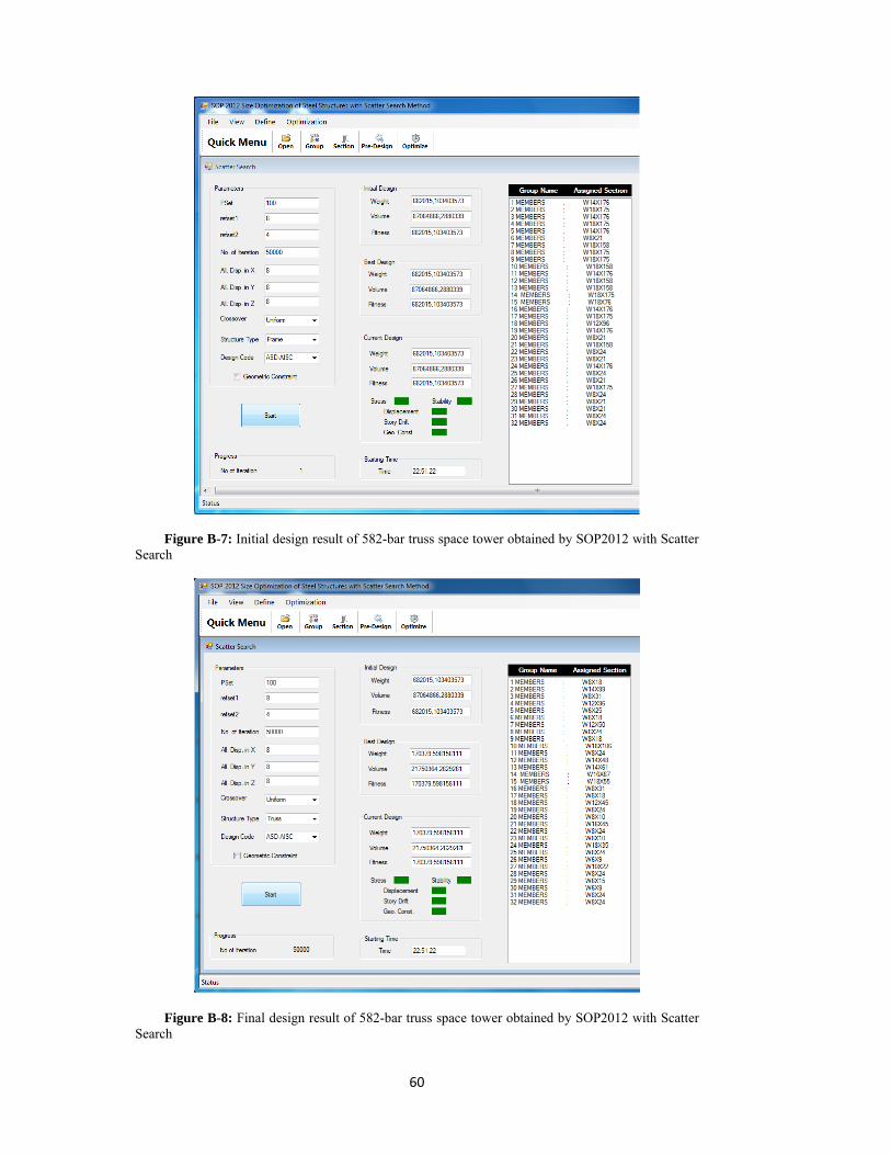
60  

Figure B-7: Initial design result of 582-bar truss space tower obtained by SOP2012 with Scatter Search

Figure B-8: Final design result of 582-bar truss space tower obtained by SOP2012 with Scatter Search

61  

693-Bar Braced Barrel Vault

Figure B-9: Analysis and design section verification in SAP2000 of 693-bar braced barrel vault results obtained by SAP2000 auto design procedure

Figure B-10: Analysis and design section verification in SAP2000 of 693-bar braced barrel vault results obtained by SOP2012 with Scatter Search

62  

Figure B-11: Initial design result of 693-bar braced barrel vault obtained by SOP2012 with Scatter Search

Figure B-12: Final design result of 693-bar braced barrel vault obtained by SOP2012 with Scatter Search

63  

132-Member 4 Story Irregular Frame

Figure B-13: Analysis and design section verification in SAP2000 of 132-member 4 story irregular frame results obtained by SAP2000 auto design procedure

Figure B-14: Analysis and design section verification in SAP2000 of 132-member 4 story irregular frame results obtained by SOP2012 with Scatter Search

64  

Figure B-15: Initial design result of 132-member 4 story irregular frame obtained by SOP2012 with Scatter Search

Figure B-16: Final design result of 132-member 4 story irregular frame obtained by SOP2012 with Scatter Search

65  

568-Member 10 Story Frame

Figure B-17: Analysis and design section verification in SAP2000 of 568-member 10 story frame results obtained by SAP2000 auto design procedure

Figure B-18: Analysis and design section verification in SAP2000 of 568-member 10 story frame results obtained by SOP2012 with Scatter Search

66  

Figure B-19: Initial design result of 568-member 10 story frame obtained by SOP2012 with Scatter Search

Figure B-20: Final design result of 568-member 10 story frame obtained by SOP2012 with Scatter Search