a population study of binocular function
TRANSCRIPT

A population study of binocular function
Article (Accepted Version)
http://sro.sussex.ac.uk
Bosten, Jenny, Goodbourn, P T, Lawrance-Owen, A J, Bargary, G, Hogg, R E and Mollon, J D (2015) A population study of binocular function. Vision Research, 110 (Part A). pp. 34-50. ISSN 0042-6989
This version is available from Sussex Research Online: http://sro.sussex.ac.uk/id/eprint/53325/
This document is made available in accordance with publisher policies and may differ from the published version or from the version of record. If you wish to cite this item you are advised to consult the publisher’s version. Please see the URL above for details on accessing the published version.
Copyright and reuse: Sussex Research Online is a digital repository of the research output of the University.
Copyright and all moral rights to the version of the paper presented here belong to the individual author(s) and/or other copyright owners. To the extent reasonable and practicable, the material made available in SRO has been checked for eligibility before being made available.
Copies of full text items generally can be reproduced, displayed or performed and given to third parties in any format or medium for personal research or study, educational, or not-for-profit purposes without prior permission or charge, provided that the authors, title and full bibliographic details are credited, a hyperlink and/or URL is given for the original metadata page and the content is not changed in any way.

A population study of binocular function Bosten JMa,b*, Goodbourn PTa,c, Lawrance-Owen AJa, Bargary Ga,d, Hogg REa,e and Mollon JDa aDepartment of Psychology, University of Cambridge, UK: [email protected] bSchool of Psychology, University of Sussex, Brighton, UK cSchool of Psychology, University of Sydney, Sydney, Australia dDivision of Optometry and Visual Science, City University, London, UK eCentre for Experimental Medicine, Queen’s University Belfast, Belfast, United Kingdom As part of a genome-wide association study (GWAS) of perceptual traits in healthy adults, we measured stereo acuity, the duration of alternative percepts in binocular rivalry and the extent of dichoptic masking in 1060 participants. We present the distributions of the measures, the correlations between measures, and their relationships to other psychophysical traits. We report sex differences, and correlations with age, interpupillary distance, eye dominance, phorias, visual acuity and personality. The GWAS, using data from 988 participants, yielded one genetic association that passed a permutation test for significance: The variant rs1022907 in the gene VTI1A was associated with self-reported ability to see autostereograms. We list a number of other suggestive genetic associations (p < 10−5). Stereo acuity; stereopsis; dichoptic masking; binocular rivalry; GWAS; individual differences 1. Introduction Human binocular function shows large individual variation. For example, stereopsis –the ability to detect binocular disparities – varies from a “hyper acuity” of few seconds of arc to complete stereo blindness. The characterization of individual differences in binocular function has the potential to yield insights into the underlying biological mechanisms (Wilmer, 2008). With the proliferation of 3D technologies, there is also practical interest in individual differences in binocular function, to ensure that the full range of binocular abilities is catered for. As part of the PERGENIC study into the genetic basis of individual differences in perception, we measured crossed and uncrossed stereo acuity, dichoptic masking and binocular rivalry in a population of 1060 normal healthy adults. Here we present population distributions for each measure, and the correlations between the measures. We also report correlations between these binocular measures, and demographic and other psychophysical measures. Genome-wide association analysis of our data has yielded a number of “suggestive” associations between the binocular measures and single nucleotide polymorphisms (p < 10−5); and one genome-wide significant association with self-reported ability to see autostereograms (p = 1.7 × 10⁻⁸). The latter association passes a permutation test. 1.1 Stereo acuity Stereo acuity is often considered a “hyper acuity”, since under optimal conditions some people are able to detect differences in binocular disparity of a few seconds of arc, differences smaller than the diameter of individual photoreceptors (Westheimer, 1975). However, there is a large range of performance across individuals. Population studies have reported estimates of median stereo acuity ranging from 12.4 to 37.2 seconds of

arc (Bohr & Read, 2013; Coutant & Westheimer, 1993; Zaroff, 2003), but between 1 and 14% of people are stereo blind (Bohr & Read, 2013; Coutant & Westheimer, 1993; Rahi, Cumberland, & Peckham, 2009; W Richards, 1970; Zaroff, 2003). Population estimates of stereo acuity and of the prevalence of deficits may be affected by the method of measurement, by the retinal location, size and duration of the targets, by differences in population sampling and by differences in exclusion criteria between studies (Heron & Lages, 2012). Poor stereopsis has a variety of known causes including strabismus, anisometropia, convergence insufficiency, early unilateral cataract, and unilateral retinal damage. It may also in some cases be caused by direct disruption of the specialist neural machinery that underlies stereopsis. Relative to other visual functions, stereo acuity seems to be disproportionately affected by aging (Wright & Wormald, 1992; Zaroff, 2003); and poor stereo acuity has been noted in vascular dementia (Mittenberg, Choi, & Apple, 2000), Electrophysiological results show that binocular visual neurons can be tuned to retinal disparities (Barlow, Blakemore, & Pettigrew, 1967). Different neural populations are tuned to crossed and uncrossed disparities, and the tuning is finest for stimuli falling close to the horopter (e.g. Poggio, 1979). Several authors have suggested that stereo acuity may be heritable, and Richards (1970) proposed an autosomal model on the basis of psychophysical data from parents and offspring. The evidence suggests that stereopsis develops in infancy between the second and sixth months of life, with crossed stereo acuity developing significantly earlier than uncrossed (Birch, Gwiazda, & Held, 1982). The development of stereopsis requires appropriate stimulation from the environment and can be disrupted by occlusion or misalignment of one eye (Blakemore, 1979; Hubel & Wiesel, 1965). However, there is some evidence to suggest that stereopsis can be acquired in adulthood (Barry, 2012). 1.2 Binocular rivalry Binocular rivalry arises when incompatible images are presented to the right and left eyes. Observers experience an alternation of percepts between the image presented to the left eye and that presented to the right. There are large individual differences in the rate of alternation, with a range spanning at least an order of magnitude (Pettigrew & Carter, 2004). Test–retest reliabilities for average percept duration are moderate to high, with past studies reporting rs = 0.69 (Whittle, 1963), rp = 0.7 (Miller et al., 2010) and rp = 0.8 (Pettigrew & Miller, 1998, in bipolar patients and controls). Variability in rate of rivalry has been found to correlate with patterns of saccadic eye movements (Hancock, Gareze, Findlay, & Andrews, 2012), with level of dichoptic masking (Baker & Graf, 2009), with retinotopic activity in extrastriate visual cortex triggered by the suppressed image (Yamashiro et al., 2014), and with variability in the structure of parietal cortex (Kanai, Bahrami, & Rees, 2010). Rate of rivalry is faster in children than adults (Hudak et al., 2011; Kovacs & Eisenberg, 2004) and declines with increasing age in adulthood (Jalavisto, 1964; Ukai, Ando, & Kuze, 2003). Rate of rivalry has been found to be reduced in bipolar disorder (Miller et al., 2003; Pettigrew & Miller, 1998; Vierck et al., 2013) and in autism (Robertson, Kravitz, Freyberg, Baron-Cohen, & Baker, 2013). Recently, Miller et al. (2010) have inferred from twin data that rate of binocular rivalry is heritable, with 52% of the variance in rivalry rate attributable to additive genetic

factors. Consistent with a reduced rate of rivalry in bipolar disorder, a candidate gene study by Schmack et al. (2013) suggested that the bipolar risk allele (2R) of the D4 dopamine receptor gene DRD4 is associated with slow perceptual switching. 1.3 Dichoptic masking In binocular or dichoptic masking, a stimulus presented to one eye is made harder to detect by a mask presented to the other. Individual differences in dichoptic masking have been noted (Baker & Meese, 2007), though to date no figure for test–retest reliability has been reported. Baker and Graf (2009) have found that individual difference in dichoptic masking are correlated with individual differences in binocular rivalry: Both within and between individuals, stronger masking is associated with longer percept durations in binocular rivalry. This association suggests the two phenomena may arise from a common suppressive process. 2. Methods Our measurements of binocular function were made as part of the PERGENIC genome-wide association study of individual differences in perceptual traits (Goodbourn et al., 2012; Lawrance-Owen et al., 2013). The PERGENIC battery consisted of about 80 perceptual measures and took about 2.5 hours for participants to complete. In the first forty minutes of the session participants were optometrically assessed, were optically corrected if necessary, and were asked to perform some standard clinical tests of vision, including the TNO test. 2.1 Participants One thousand and sixty participants (647 female) took part in the PERGENIC study. They were recruited from the Cambridge area, and many were students at the University of Cambridge. They were paid £25 for taking part. A subset of 105 participants, selected at random, returned for testing in a second session at least one week after the first session, allowing us to measure test–retest reliabilities. Participants were corrected to best optical acuity at the beginning of the session, and were given lenses to wear if acuity improved by at least 0.1 logMAR with the correction. Two hundred and thirty-four participants were given lenses for both eyes, and 110 participants were given lenses for one eye only. As a preliminary measure to guard against population stratification, all participants in our sample were of self-reported European origin. The study was approved by the Cambridge Psychology Research Ethics Committee, and was carried out in accordance with the tenants of the Declaration of Helsinki. All participants gave written informed consent before taking part. 2.2 Visual acuity, sighting dominant eye, pupil size, inter-pupillary distance and phoria Monocular and binocular logMAR visual acuity was measured using an EDTRS chart before and after a refraction using a standardized protocol. We measured sighting dominant eye by a variant of the Miles test (Miles, 1929). Participants were seated facing a Snellen chart for measuring acuity, and asked to stretch out both arms, creating a small aperture with the thumbs and index fingers of both hands. They were asked to fixate on a letter on the chart through the aperture and then, keeping both eyes open, to bring their hands slowly towards their face. The
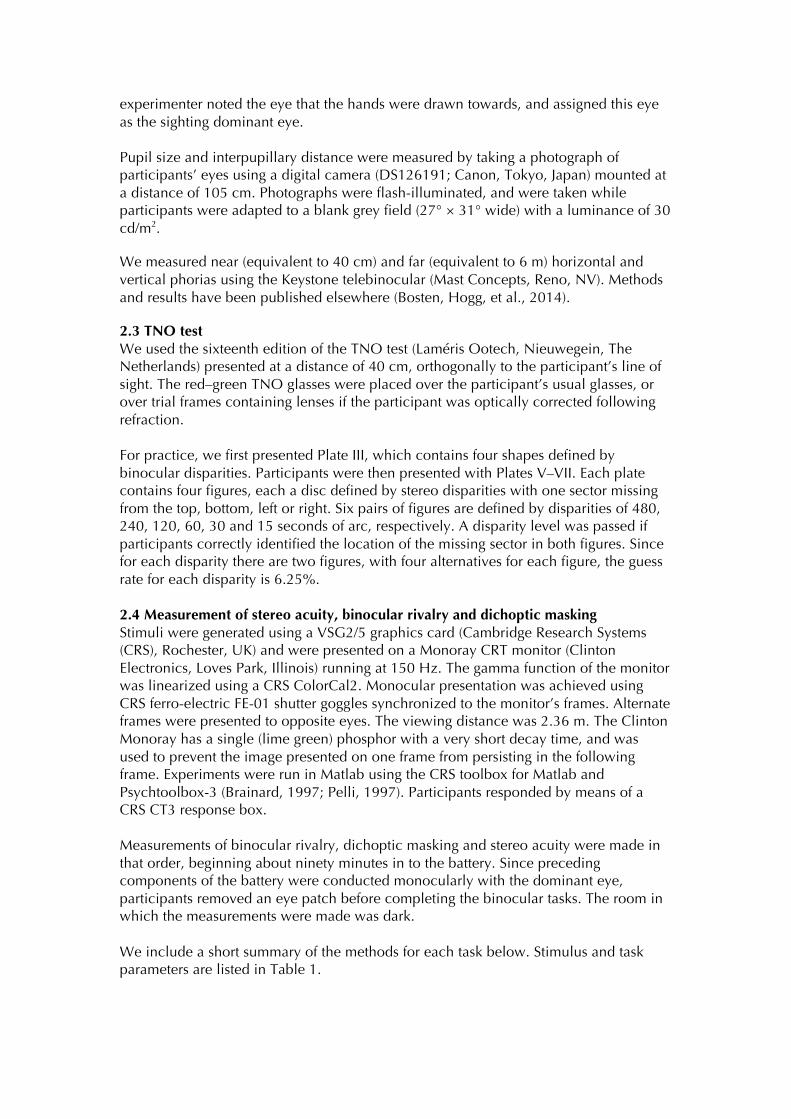
experimenter noted the eye that the hands were drawn towards, and assigned this eye as the sighting dominant eye. Pupil size and interpupillary distance were measured by taking a photograph of participants’ eyes using a digital camera (DS126191; Canon, Tokyo, Japan) mounted at a distance of 105 cm. Photographs were flash-illuminated, and were taken while participants were adapted to a blank grey field (27° × 31° wide) with a luminance of 30 cd/m2.
We measured near (equivalent to 40 cm) and far (equivalent to 6 m) horizontal and vertical phorias using the Keystone telebinocular (Mast Concepts, Reno, NV). Methods and results have been published elsewhere (Bosten, Hogg, et al., 2014).
2.3 TNO test We used the sixteenth edition of the TNO test (Laméris Ootech, Nieuwegein, The Netherlands) presented at a distance of 40 cm, orthogonally to the participant’s line of sight. The red–green TNO glasses were placed over the participant’s usual glasses, or over trial frames containing lenses if the participant was optically corrected following refraction. For practice, we first presented Plate III, which contains four shapes defined by binocular disparities. Participants were then presented with Plates V–VII. Each plate contains four figures, each a disc defined by stereo disparities with one sector missing from the top, bottom, left or right. Six pairs of figures are defined by disparities of 480, 240, 120, 60, 30 and 15 seconds of arc, respectively. A disparity level was passed if participants correctly identified the location of the missing sector in both figures. Since for each disparity there are two figures, with four alternatives for each figure, the guess rate for each disparity is 6.25%. 2.4 Measurement of stereo acuity, binocular rivalry and dichoptic masking Stimuli were generated using a VSG2/5 graphics card (Cambridge Research Systems (CRS), Rochester, UK) and were presented on a Monoray CRT monitor (Clinton Electronics, Loves Park, Illinois) running at 150 Hz. The gamma function of the monitor was linearized using a CRS ColorCal2. Monocular presentation was achieved using CRS ferro-electric FE-01 shutter goggles synchronized to the monitor’s frames. Alternate frames were presented to opposite eyes. The viewing distance was 2.36 m. The Clinton Monoray has a single (lime green) phosphor with a very short decay time, and was used to prevent the image presented on one frame from persisting in the following frame. Experiments were run in Matlab using the CRS toolbox for Matlab and Psychtoolbox-3 (Brainard, 1997; Pelli, 1997). Participants responded by means of a CRS CT3 response box. Measurements of binocular rivalry, dichoptic masking and stereo acuity were made in that order, beginning about ninety minutes in to the battery. Since preceding components of the battery were conducted monocularly with the dominant eye, participants removed an eye patch before completing the binocular tasks. The room in which the measurements were made was dark. We include a short summary of the methods for each task below. Stimulus and task parameters are listed in Table 1.

Table 1. Stimulus and task parameters for crossed and uncrossed stereo acuity, binocular rivalry and dichoptically masked and unmasked contrast sensitivity. Crossed and uncrossed stereo
acuity Binocular rivalry Dichoptically masked and unmasked contrast
sensitivity Stimulus geometry (°)
Ring eccentricity: 0.7 Ring diameter: 0.2 SD of Gaussian: 0.02 Fixation cross: 0.15 x 0.15 Fixation cross stroke: 0.02 Black surround: 2.7 x 2.7 Noise field: 5.8 x 5.8 Noise pixels: 0.06 x 0.06
Grating size: 2 x 2 Grating patial frequency: 2 c.p.d Fixation cross: 0.08 x 0.08 Fixation cross stroke: 0.01
Grating size: 1.26 x 1.26 Grating spatial frequency: 3 c.p.d. Grating eccentricity: 2 Fixation cross: 0.08 x 0.08 Fixation cross stroke: 0.01
Stimulus luminance (cd/m2)
Mean of noise field: 48 Ring (peak): 48 Fixation cross: 97
Mean of grating: 39 Background: 39
Contrast of masking gratings: 0.25 Mean of masking gratings: 39 Mean of test and distractor gratings: 39 Background: 19 Blank squares in inter-trial-interval: 39
Stimulus contrast
Noise field: ~1 Grating: 0.75 Masking gratings: 0.25
Presentation time
Until response had been received 2 minutes 200 ms
Auditory feedback:
Correct: Two 100-ms high tones Incorrect: One 100-ms low tone
A short tone of medium pitch indicated response reception
Correct: Two 100-ms high tones Incorrect: One 100-ms low tone
Training Constant disparity of 140 seconds of arc. Terminated after 8 consecutive correct responses or 60 trials.
Unmasked contrast sensitivity: Target gratings at close to full contrast. Terminated after 3 consecutive correct responses. Masked contrast sensitivity: Target gratings at 0.25. Presentation time decreased from 1500 ms, to 750 ms and then to 200 ms, each after 3 consecutive correct responses. Terminated after 5 consecutive correct responses at 200 ms.
Test blocks 4: Two for crossed disparities, two for uncrossed disparities. Order: ABBA or BAAB.
1 1
Staircases Starting disparity: 245 seconds of arc Maximum disparity: 250 seconds of arc Trials per staircase: 25
N/A Starting contrast: 0.63 Trials per staircase: 25 (unmasked); 30 (masked)
Analysis Data were combined from the 2 staircases for each disparity type. Threshold was defined as the 67% point on the psychometric function.
Data were combined from the 2 staircases for eye. Threshold was defined as the 70% point on the psychometric function.
2.5 Crossed and uncrossed stereo acuity A representation of the stimulus for measuring stereo acuity is given in Figure 1(a). Four Gaussian rings were presented around a central fixation cross, on a square black surround embedded in a square field of pixelated binary random noise, included to aid binocular fusion. The stimuli were identical in the two eyes, except for the position of one of the four Gaussian rings. The separation between the two rings (the binocular disparity) was decided on each trial by a staircase procedure. There was random jitter in the horizontal position of each ring, to prevent the participant completing the task by selecting the ring that had an eccentricity different from the others. The jitter for each ring was randomly assigned on each trial. It was uniformly distributed with a maximum of ±175 seconds of arc. The participant was given the following instructions on the screen: “The goggles you are looking through are 3D goggles. You will see four rings on each trial, and one of the rings should appear to be at a different depth to the others. Your task is to press the button corresponding to the ring that is at a different depth from the others.” Two

examples were then shown, in which one of the rings had either a crossed or an uncrossed binocular disparity of 245 seconds of arc. The participant was instructed to alert the experimenter (by pressing a buzzer) if one ring in each example did not clearly look to be at a different depth from the others. If the experimenter was alerted, he or she entered the experimental room and identified the ring that should appear to be in depth, encouraging the participant to perceive the disparity signal. Whether or not depth was subsequently perceived, the participant then progressed to the main part of the experiment. Following the examples there was a training phase, first for crossed disparities, and then for uncrossed disparities. In the testing phase, thresholds for crossed and uncrossed binocular disparities were measured in separate blocks. According to the block, the participant was instructed to identify on each trial the ring that was either nearer or further than the others. The stimulus remained on screen until the participant had made a response. The disparity on each trial was decided by a ZEST staircase (King-Smith, Grigsby, Vingrys, Benes, & Supowit, 1994; Watson & Pelli, 1983) according to the participant’s responses. The Gaussian luminance profile of the ring stimuli allowed antialiasing, so that disparities smaller than one pixel could be presented.
Figure 1. Stimuli. Panel (a) shows an example of a stimulus for stereo acuity. The target (the top ring here) has a stereo disparity, and two rings are visible in the figure as the rings presented to the right and left eyes have been superimposed. The other three rings have no stereo disparity. Panel (b) shows the stimulus for dichoptic masking. Gratings were presented for 200 ms. The target was oriented orthogonally to the three distractor gratings (presented to the same eye) and the four masking gratings (presented to the opposite eye). Here, the target is the left grating presented to the right eye. 2.6 Binocular rivalry Binocular rivalry was measured at the beginning of the battery of tests of binocular function, but after rivalry for ambiguous figures had already been measured in the previous testing room. The stimuli were centrally presented sinusoidal gratings inside squares. The grating presented to the left eye was oriented along the negative diagonal, and the grating presented to the right eye was oriented along the positive diagonal. There was a central black fixation cross presented to both eyes. Participants were instructed that diagonal gratings of different orientations would be presented to the two eyes. They were told that at some times they would see a grating tilted to the left and at other times they would see the grating tilted to the right. They
x
left eye
right eye
300 ms 200 ms ≤ 5 seconds
x x
xxx
(a) (b)
were instructed to press the left button if they perceived a grating oriented along the negative diagonal and the right button if they perceived a grating oriented along the positive diagonal. They were instructed that in the case of mixed percepts, they should judge the grating that covered most of the square. They were instructed to maintain fixation on the central cross at all times. Both gratings were presented for a period of two minutes. 2.7 Dichoptic masking A representation of the stimulus for dichoptic masking is given in Figure 1(b). The stimulus for measuring unmasked contrast thresholds was the same as for dichoptic masking, but without the mask and the distractor gratings. Stimuli were four sinusoidal gratings oriented along the positive diagonal, presented around a central black fixation cross. The masking gratings were presented to one eye. The test grating was presented to the other eye, at one of the four positions of the masking gratings. It was identical to the masking gratings, except it was oriented along the negative diagonal. Distractor gratings oriented along the positive diagonal were presented at the remaining three positions. The contrast of the test and distractor gratings was decided on each trial by a ZEST staircase. On each trial, prior to and following the presentation of the test and masking gratings there were four blank squares presented at the same locations. Both eyes were tested: Thresholds were measured for contrast in the left eye masked by a stimulus presented to the right eye and vice versa. Unmasked contrast thresholds were measured first. Participants were told that they would see a grating flashed inside one of four squares, and were instructed to press the button that corresponded to the position of the grating. There was a short training period (Table 1), Immediately following training, four interleaved ZEST staircases (two for each eye) tracked the participant’s threshold contrast. On each trial, following presentation of the test stimulus, the participant had up to 5 s to respond. The next trial began after 5 s or following the participant’s response. For measurement of dichoptically masked contrast thresholds, unmasked contrast threshold was not used to adjust the contrast of the mask, as we wanted all participants to receive the same physical stimulus. During a period of training (Table 1), the eye of presentation of the test and masking gratings was decided at random on each trial. Following training, four interleaved ZEST staircases (two for each eye) converged on a participant’s dichoptically masked thresholds. 2.8 Other psychophysical measures We correlated our binocular measures with other psychophysical measures in the PERGENIC test battery, including
1. Detection of gratings of low spatial frequency presented on pulsed and steady pedestals detection of gratings on steady pedestals is discussed in Goodbourn et al. (2012). Detection on a pulsed pedestal used the same method but there was a luminance pedestal (∆I) of 5.3 cd/m2 temporally coincidental with the target grating
2. Detection of coherent motion (Goodbourn et al., 2012). 3. Detection of gratings of low spatial and high temporal frequency (Goodbourn et
al., 2014; Goodbourn et al., 2012).

4. Performance on the Pelli–Robson test (Pelli, Robson & Wilkins, 1988) 5. Detection of S-cone increments and decrements (Bosten, Bargary, et al., 2014;
Goodbourn et al., 2012) 6. Detection of differences in the frequency, duration and order of auditory stimuli
(auditory order is discussed in Goodbourn et al., 2012), and detection of coherent form.
Methods for these measures have already been published, except for detection of differences in auditory frequency and duration, and detection of coherent form. We include brief methods for these below. 2.8.1 Detection of differences in auditory frequency and duration For the auditory frequency task the stimuli were three consecutive tones (peak intensity 65 dB sound pressure level (SPL)) with onsets 0.5 s apart: a reference tone (TR) and two test tones (T1 and T2). TR was a pure sinusoid (440 Hz) of 250 ms duration, with intensity ramped on and off over 10ms. On each trial, one of T1 or T2 matched TR exactly, while the other had a higher frequency. The frequency of the oddball tone was varied adaptively between trials. The participant's task was to identify which of T1 or T2 differed from TR. For the auditory duration task the stimuli were three consecutive tones with onsets 550 ms apart. On each trial, one of T1 or T2 matched TR exactly, while the other had a longer duration. The duration of the oddball tone was varied adaptively between trials. The participant's task was to identify which of T1 or T2 differed from TR. Both tasks were two-alternative forced-choice. Participants completed a set of practice trials to ensure they understood the task. For experimental trials, test intensity was determined according to two independent interleaved ZEST staircases, terminated after 30 trials. Feedback was provided by colored lights. Auditory stimuli were played binaurally via an M-Audio Fast Track USB sound card at a 48 kHz sample rate through Sennheiser HD205 circumaural stereo headphones. 2.8.2 Detection of coherent form Stimuli comprised 0.04° white dots (10% density) within an annulus of inner radius 1.0° and outer radius 10.0°. Background luminance was 30 cd/m2 and dot luminance was 60 cd/m2. The fixation marker was positioned in the centre of the annulus. In each block of trials, orientation information was introduced by one of two methods. In one task, streaks were formed by arranging dots in a Glass pattern (Glass, 1969). Each seed dot in a random array was paired with a daughter dot located 0.5° away. A proportion of signal dots were displaced from the seed dot in the target direction (either upwards and to the left, or upwards and to the right), and remaining dots were displaced in random directions. The proportion of signal dots was varied adaptively between trials. In the other task, stripes were created by modulating dot density across space according to a sine wave (fS = 1.0 c deg−1, φ randomized). The axis of modulation was either from the lower right to the upper left, or from the lower left to the upper right. The amplitude of density modulation was varied adaptively between trials. The participant’s task was to identify the direction in which the texture was tilted (45° to the left or right from vertical). The tasks were two-alternative forced-choice. Participants completed a set of practice trials to ensure they understood the task. For experimental trials, test intensity was

determined according to two independent ZEST staircases, blocked in ABBA order. Staircases terminated after 50 trials. Feedback in the form of auditory tones was provided throughout. Experiments were conducted in a darkened room. All stimuli were generated using Matlab R2007b software with PsychToolbox-3. Responses were collected using a two-button hand-held box. Stimuli were displayed via a specialized video processor (BITS++; Cambridge Research Systems, Rochester, UK) on a gamma-corrected Sony Trinitron monitor operating at 100 Hz. Observers viewed stimuli monocularly using their preferred eye, or—if the difference in visual acuity between eyes was 0.10 logMAR or greater—using the eye with better acuity. They used a headrest to maintain a viewing distance of 0.5 m. 2.9 Questionnaires Before coming to the lab for testing, participants completed a 75-item online questionnaire. Included in the questionnaire were items to gather demographic information (age, sex, ancestry), the mini IPIP to measure the ‘Big 5’ personality traits (Donnellan, Oswalk, Baird, & Lucas, 2006), and items about various visual and auditory attributes. Most relevant for binocular function was an item on ability to see autostereograms: “I am good at seeing Magic Eye puzzles (stereograms).” Participants were required to rate their agreement with the statement on a Likert scale ranging from 1 (strongly disagree) to 5 (strongly agree). We assessed handedness via two questionnaire items, also using a Likert scale. One was “I always use my right hand when writing”; the other, “I always throw a ball with my right hand”. Handedness was quantified as the average Likert score for the two questions. A subset of 555 participants completed a second online questionnaire, about 6 months after completing the psychophysical tests. The second questionnaire included a set of 50 items to measure the Autism Quotient (Baron-Cohen, Wheelwright, Skinner, Martin, & Clubley, 2001). 2.10 GWAS methods Each participant provided a saliva sample using Oragene OG-500 DNA kits (DNA Genotek Inc., Ottawa, Canada). After extraction of DNA, 1008 samples were genotyped using Illumina Human OmniExpress arrays. The BeadChip allowed characterization of 733,202 SNPs. Genotype calling was by custom clustering using GenomeStudio software (Illumina Inc, San Diego, CA). We excluded 20 individuals from the genetic data set following genotyping. For one there was a low call rate; three had sex anomalies; 15 were related individuals or duplicate samples; and one was a population outlier. Nine hundred and eighty-eight individuals remained in the GWAS. We excluded 12.3% of genotyped SNPs. These markers either had greater than 2% missing genotypes (N = 12,706), or had a minor allele frequency below 1% (N = 77,738). After exclusions, 642,758 SNPs remained in the analysis. For each SNP we conducted a quantitative trait analysis using PLINK (Purcell et al., 2007), using ranked data for each phenotype. To control for any residual population stratification in our sample, we used EIGENSOFT (Price et al., 2006) to extract the first three principal components (PCs) of genetic variation. The three PCs were entered, along with sex, as covariates in the regression model for each phenotype.

For each locus that the quantitative trait analysis found to be suggestively associated (p < 10−5), we ran a whole-genome permutation procedure using PLINK: The phenotype–genotype correspondences in our data were randomly shuffled, and genetic association analyses were run for all genotyped SNPs in each of 10 000 permutations. To control for population stratification in the permutation analysis we allowed shuffling only within genetic clusters of participants, identified by PLINK’s clustering facility with identity-by-state as the distance metric. The permuted p-value for each SNP is the proportion of permutations on which the test statistic for any SNP exceeds the test statistic found in the original (unpermuted) association analysis for that particular SNP. The whole-genome permuted p-value is a conservative empirical control for type 1 errors. We imputed SNPs within a 2.5-Mbp region of interest centered on each suggestively associated SNP (P < 10−5) using IMPUTE2 (Howie, Marchini, & Stephens, 2011; Howie, Donnelly, & Marchini, 2009) with the 1000 genomes phased haplotypes (Abecasis et al., 2010). Association analyses of the imputed regions were performed using PLINK, with sex and the three PCs as covariates, as for the analysis of genotyped SNPs. Finally, we did a clustering analysis using PLINK’s clumping function, with a significance threshold for index SNPs of p = 10−5, a significance threshold for clustered SNPs of p = 0.01, a linkage disequilibrium (LD) threshold for clustering of r2 = 0.1, and a physical distance threshold for clustering of 1250 kbp. Clustering defines a region that is in LD with the locus of interest, and which contains other SNPs (the “clustered” SNPs) that are associated with the trait with a specified p-value. The clustered region therefore defines a region in which the polymorphism causally associated with the phenotype is likely to lie.
3. Results 3.1 Exclusions For our adaptive test of stereo acuity, we made no exclusions to the data presented in sections 3.2–3.5. For the TNO test two participants’ data were missing at the point of collection. For binocular rivalry, nine participants’ data were excluded because they made only one button press during the recording session. For unmasked contrast detection, participants’ data were excluded if they did not achieve threshold even at a contrast of 1. There were 17 exclusions for the right eye only and 16 exclusions for the left eye only; an additional 27 participants had data excluded for both eyes. Many participants who had data excluded only for one eye had an identifiable binocular problem such as amblyopia, strabismus, retinal scarring or macular edema. We presume that the participants who performed at the floor on both eyes did not understand the task. A possible reason was that binocular rivalry was run directly before unmasked contrast, and if participants failed to read the instructions, they may have attempted to map the responses required for binocular rivalry (left and right judgments of tilt) on to the unmasked contrast task (four alternative spatial forced choice). For dichoptically masked contrast detection, participants’ data were excluded if they did not achieve threshold even at a contrast of 1. There were 3 exclusions for the right eye only and 8 for the left only. 3.2 Test–retest reliabilities One hundred and five participants were randomly selected to return for testing in a second session. Data from some participants were missing or excluded (section 3.1); the n in Table 2 indicates, for each measure, the number of participants on which test–
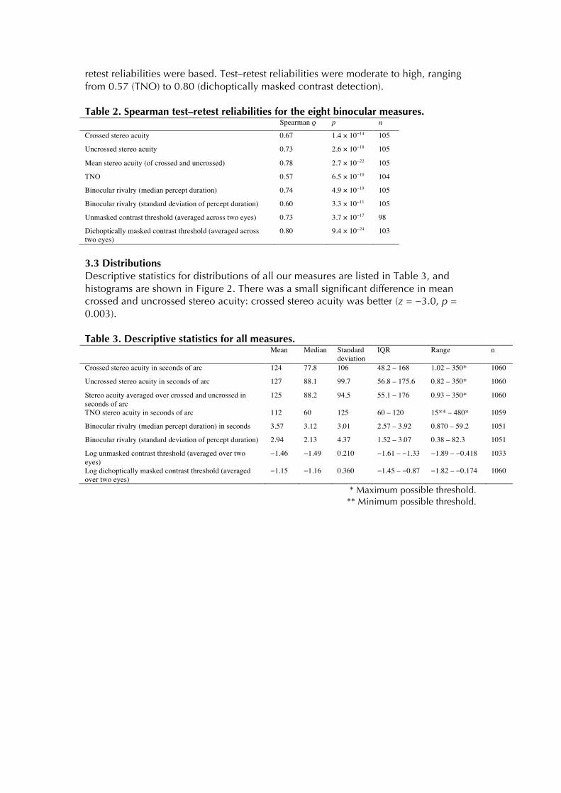
retest reliabilities were based. Test–retest reliabilities were moderate to high, ranging from 0.57 (TNO) to 0.80 (dichoptically masked contrast detection). Table 2. Spearman test–retest reliabilities for the eight binocular measures. Spearman ρ p n
Crossed stereo acuity 0.67 1.4 × 10⁻¹⁴ 105
Uncrossed stereo acuity 0.73 2.6 × 10⁻¹⁸ 105
Mean stereo acuity (of crossed and uncrossed) 0.78 2.7 × 10⁻²² 105
TNO 0.57 6.5 × 10⁻¹⁰ 104
Binocular rivalry (median percept duration) 0.74 4.9 × 10⁻¹⁹ 105
Binocular rivalry (standard deviation of percept duration) 0.60 3.3 × 10⁻¹¹ 105
Unmasked contrast threshold (averaged across two eyes) 0.73 3.7 × 10⁻¹⁷ 98
Dichoptically masked contrast threshold (averaged across two eyes)
0.80 9.4 × 10⁻²⁴ 103
3.3 Distributions Descriptive statistics for distributions of all our measures are listed in Table 3, and histograms are shown in Figure 2. There was a small significant difference in mean crossed and uncrossed stereo acuity: crossed stereo acuity was better (z = −3.0, p = 0.003). Table 3. Descriptive statistics for all measures. Mean Median Standard
deviation IQR Range n
Crossed stereo acuity in seconds of arc 124 77.8 106 48.2 – 168 1.02 – 350* 1060
Uncrossed stereo acuity in seconds of arc 127 88.1 99.7 56.8 – 175.6 0.82 – 350* 1060
Stereo acuity averaged over crossed and uncrossed in seconds of arc
125 88.2 94.5 55.1 – 176 0.93 – 350* 1060
TNO stereo acuity in seconds of arc 112 60 125 60 – 120 15** – 480* 1059
Binocular rivalry (median percept duration) in seconds 3.57 3.12 3.01 2.57 – 3.92 0.870 – 59.2 1051
Binocular rivalry (standard deviation of percept duration) 2.94 2.13 4.37 1.52 – 3.07 0.38 – 82.3 1051
Log unmasked contrast threshold (averaged over two eyes)
−1.46 −1.49 0.210 −1.61 – −1.33 −1.89 – −0.418 1033
Log dichoptically masked contrast threshold (averaged over two eyes)
−1.15 −1.16 0.360 −1.45 – −0.87 −1.82 – −0.174 1060
* Maximum possible threshold. ** Minimum possible threshold.
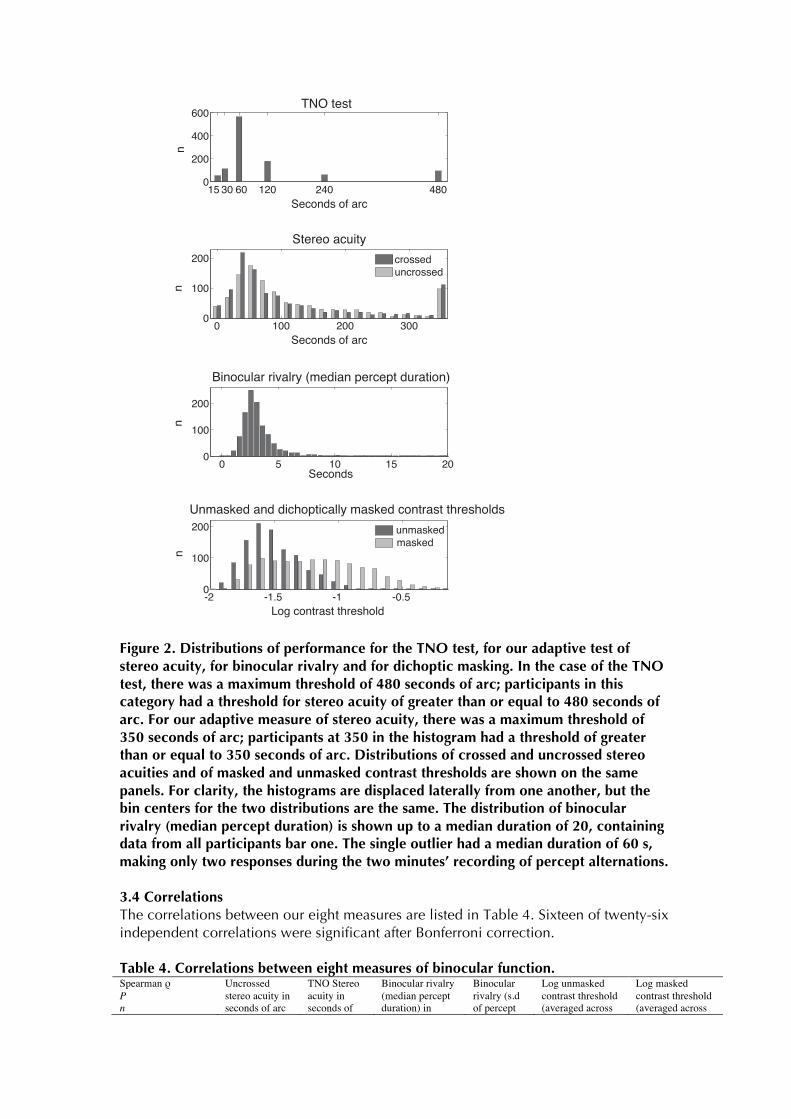
Figure 2. Distributions of performance for the TNO test, for our adaptive test of stereo acuity, for binocular rivalry and for dichoptic masking. In the case of the TNO test, there was a maximum threshold of 480 seconds of arc; participants in this category had a threshold for stereo acuity of greater than or equal to 480 seconds of arc. For our adaptive measure of stereo acuity, there was a maximum threshold of 350 seconds of arc; participants at 350 in the histogram had a threshold of greater than or equal to 350 seconds of arc. Distributions of crossed and uncrossed stereo acuities and of masked and unmasked contrast thresholds are shown on the same panels. For clarity, the histograms are displaced laterally from one another, but the bin centers for the two distributions are the same. The distribution of binocular rivalry (median percept duration) is shown up to a median duration of 20, containing data from all participants bar one. The single outlier had a median duration of 60 s, making only two responses during the two minutes’ recording of percept alternations. 3.4 Correlations The correlations between our eight measures are listed in Table 4. Sixteen of twenty-six independent correlations were significant after Bonferroni correction. Table 4. Correlations between eight measures of binocular function. Spearman ρ P n
Uncrossed stereo acuity in seconds of arc
TNO Stereo acuity in seconds of
Binocular rivalry (median percept duration) in
Binocular rivalry (s.d of percept
Log unmasked contrast threshold (averaged across
Log masked contrast threshold (averaged across
-2 -1.5 -1 -0.50
100
200
a
a
unmaskedmasked
0 5 10 15 200
100
200
a
a
0 100 200 3000
100
200
a
a
crosseduncrossed
15 30 60 120 240 4800
200
400
600
a
TNO test
������Stereo acuity
Seconds of arc
n
Seconds of arc
n
Binocular rivalry (median percept duration)
Seconds
nn
Log contrast threshold
Unmasked and dichoptically masked contrast thresholds
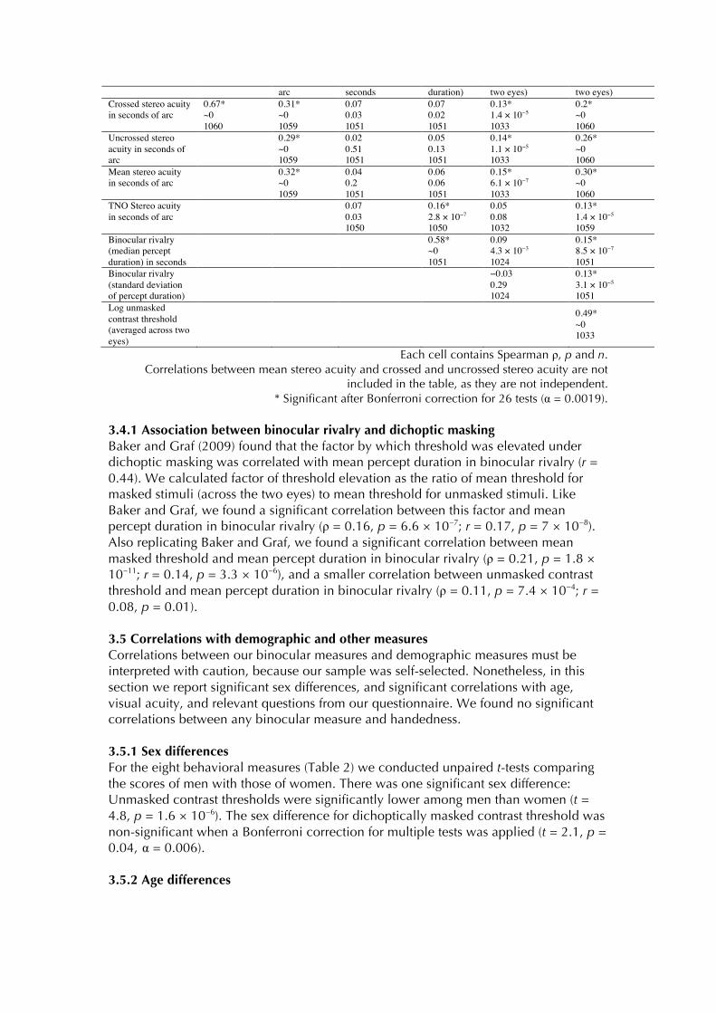
arc seconds duration) two eyes) two eyes) Crossed stereo acuity in seconds of arc
0.67* ~0 1060
0.31* ~0 1059
0.07 0.03 1051
0.07 0.02 1051
0.13* 1.4 × 10−5
1033
0.2* ~0 1060
Uncrossed stereo acuity in seconds of arc
0.29* ~0 1059
0.02 0.51 1051
0.05 0.13 1051
0.14* 1.1 × 10−5
1033
0.26* ~0 1060
Mean stereo acuity in seconds of arc
0.32* ~0 1059
0.04 0.2 1051
0.06 0.06 1051
0.15* 6.1 × 10−7
1033
0.30* ~0 1060
TNO Stereo acuity in seconds of arc
0.07 0.03 1050
0.16* 2.8 × 10−7
1050
0.05 0.08 1032
0.13* 1.4 × 10−5
1059 Binocular rivalry (median percept duration) in seconds
0.58* ~0 1051
0.09 4.3 × 10⁻³
1024
0.15* 8.5 × 10−7
1051 Binocular rivalry (standard deviation of percept duration)
−0.03 0.29 1024
0.13* 3.1 × 10−5
1051 Log unmasked contrast threshold (averaged across two eyes)
0.49* ~0 1033
Each cell contains Spearman ρ, p and n. Correlations between mean stereo acuity and crossed and uncrossed stereo acuity are not
included in the table, as they are not independent. * Significant after Bonferroni correction for 26 tests (α = 0.0019).
3.4.1 Association between binocular rivalry and dichoptic masking Baker and Graf (2009) found that the factor by which threshold was elevated under dichoptic masking was correlated with mean percept duration in binocular rivalry (r = 0.44). We calculated factor of threshold elevation as the ratio of mean threshold for masked stimuli (across the two eyes) to mean threshold for unmasked stimuli. Like Baker and Graf, we found a significant correlation between this factor and mean percept duration in binocular rivalry (ρ = 0.16, p = 6.6 × 10⁻⁷; r = 0.17, p = 7 × 10⁻⁸). Also replicating Baker and Graf, we found a significant correlation between mean masked threshold and mean percept duration in binocular rivalry (ρ = 0.21, p = 1.8 × 10⁻¹¹; r = 0.14, p = 3.3 × 10⁻⁶), and a smaller correlation between unmasked contrast threshold and mean percept duration in binocular rivalry (ρ = 0.11, p = 7.4 × 10⁻⁴; r = 0.08, p = 0.01). 3.5 Correlations with demographic and other measures Correlations between our binocular measures and demographic measures must be interpreted with caution, because our sample was self-selected. Nonetheless, in this section we report significant sex differences, and significant correlations with age, visual acuity, and relevant questions from our questionnaire. We found no significant correlations between any binocular measure and handedness. 3.5.1 Sex differences For the eight behavioral measures (Table 2) we conducted unpaired t-tests comparing the scores of men with those of women. There was one significant sex difference: Unmasked contrast thresholds were significantly lower among men than women (t = 4.8, p = 1.6 × 10⁻⁶). The sex difference for dichoptically masked contrast threshold was non-significant when a Bonferroni correction for multiple tests was applied (t = 2.1, p = 0.04, α = 0.006). 3.5.2 Age differences

Median percept duration in binocular rivalry was significantly correlated with age (ρ = 0.14, p = 2.6 × 10⁻⁶): Older individuals had longer median percept durations. This correlation was observed despite the age restriction on our sample of 16–40 years. 3.5.3 Visual acuity When vision was uncorrected or with usual optical correction, the mean binocular acuity in our sample was −0.152 logMAR, with a standard deviation of 0.10 logMAR and a range −0.30 logMAR (the minimum the chart could measure) to 0.60 logMAR. Giving 334 participants lenses (in addition to their usual correction, if applicable) improved mean acuity in the whole sample to −0.176 logMAR, and the range to −0.3–0.06 logMAR. Table 5 shows that our binocular measures, with the exception of median percept duration in binocular rivalry, were significantly correlated with binocular visual acuity (either uncorrected or with usual correction). Stereo thresholds were significantly correlated with the absolute difference in visual acuity (with usual correction) between the two eyes (mean: 0.046 logMAR, std: 0.081 logMAR), such that a greater interocular difference in acuity was associated with higher stereo thresholds. Median percept duration in binocular rivalry was also significantly correlated with the absolute difference in acuity between the two eyes. The stimulus presented to the eye with better acuity was perceived for a significantly greater proportion of the time than the stimulus presented to the eye with worse acuity (medians 0.529 vs. 0.471; t = 4.65, p = 3.8 × 10⁻⁶). Unmasked contrast thresholds were significantly lower in the eye of best-corrected optical acuity than in the worse eye (t = 2.25, p = 0.025). Thresholds for masked stimuli were significantly lower if the target was presented to the strong eye and the mask to the weak eye than vice versa (t = 3.05, p = 0.0024). Table 5. Correlations between the binocular measures and visual acuity. ρ, p Binocular
visual acuity (usual correction)
Binocular visual acuity (best corrected)
Acuity in better eye (best corrected)
Acuity in worse eye (best corrected)
Absolute interocular acuity difference
TNO Stereo acuity 0.16, 5.1 × 10⁻⁷ 0.20, 9.9 × 10⁻¹¹ 0.16, 4.5 × 10⁻⁷ 0.36, 4.8 × 10⁻³³ 0.33, 5.3 × 10⁻²⁸ Stereo acuity averaged over crossed and uncrossed 0.16, 1.2 × 10⁻⁶ 0.15, 3.7 × 10⁻⁶ 0.11, 4.7 × 10⁻⁴ 0.24, 2.0 × 10⁻¹⁵ 0.22, 6.3 × 10⁻¹³ Unmasked contrast threshold 0.14, 4.1 × 10⁻⁵ 0.18, 6.5 × 10⁻⁸ 0.17, 4.4 × 10⁻⁸ 0.09, 2.7 × 10⁻³ -0.07, 0.03 Dichoptically masked contrast threshold 0.16, 9.9 × 10⁻⁷ 0.18, 7.5 × 10⁻⁹ 0.16, 8.1 × 10⁻⁸ 0.14, 3.6 × 10⁻⁶ 0.03, 0.37 Binocular rivalry (median percept duration) 0.03, 0.35 0.08, 0.02 0.05, 0.11 0.16, 8.7 × 10⁻⁸ 0.18, 7.4 × 10⁻⁹ 3.5.4 Amblyopia If the absolute difference in optimally corrected visual acuity between the two eyes was greater than 0.2 logMAR, we defined the participant as an amblyope. Twenty-eight participants met this criterion. Stereo acuity was significantly worse for amblyopes than for non-amblyopes (t = 5.9, p ~0 for stereo acuity averaged over crossed and uncrossed; t = 9.7, p ~0 for TNO stereo acuity. On the TNO test, mean stereo acuity was 106.1 seconds of arc for non-amblyopes, and 327.8 seconds of arc for amblyopes. For our adaptive test, mean stereo acuity was 122.6 seconds of arc for non-amblyopes and 228.2 seconds of arc for amblyopes. The greater difference between the two groups on the TNO test than on the adaptive test may be because the stimuli of the former contain higher spatial frequencies. Mean percept duration in binocular rivalry was significantly longer for amblyopes than for non-amblyopes (T = 6.0, p = 2.7 x 10⁻⁹). Though there was no difference in mean dichoptically masked contrast thresholds between groups, dichoptically masked

contrast thresholds were significantly greater when the detection stimulus was presented to the amblyope’s weak eye than when it was presented to the strong eye (t = 5.5, p = 1.2 × 10⁻⁶). Amblyopes experience greater dichoptic masking than normal if the mask is presented to their strong eye, but reduced dichoptic masking than normal if the mask is presented to their weak eye. 3.5.5 Sighting eye dominance Sighting eye dominance was available for 988 participants. Of these, 627 (64%) were right-eye dominant. We found no significant differences between right- and left-eye dominant participants for our binocular measures listed in Table 2. There were no significant differences in binocularly masked or unmasked contrast thresholds in the dominant eye compared to the non-dominant eye. In binocular rivalry the stimulus that was presented to the dominant eye was perceived for a significantly greater proportion of time than the stimulus that was presented to the non-dominant eye (t = 3.3, p = 9.3 × 10⁻⁴). The mean proportion of the time the stimulus that was presented to the dominant eye was perceived was 0.516; the median was 0.515. 3.5.6 Inter-pupillary distance There was a small positive correlation between stereo acuity measured using the TNO test and inter-pupillary distance (ρ = 0.07, p = 0.02). From inspection of the scatter plots, there was no evidence of a non-linear relationship between inter-pupillary distance and stereo acuity measured either using the TNO or using our own adaptive test. There was a significant negative correlation between inter-pupillary distance and unmasked contrast threshold averaged across the two eyes (ρ = −0.12, p = 0.0002), but not between inter-pupillary distance and dichoptically masked contrast threshold. 3.5.7 Phorias We correlated near and far vertical and horizontal phorias with our different measures of stereo acuity. Phoria is on a scale from large negative deviations (esophoria) to large positive deviations (exophoria). We also correlated stereo acuity and absolute phoria, in order to test the hypothesis that stereo acuity might be impaired by a large deviation in either direction. Correlations are given in Table 6. Most correlations are surprisingly low. There are four significant correlations between phorias and stereo acuity measured using the TNO test. Stereo acuity decreases with increasing absolute vertical phoria, and increases with increasing raw horizontal phoria. Similarly, crossed stereo acuity increases with increasing horizontal phoria when measured using our own adaptive test, but only significantly for far phoria. Table 6. Correlations between stereo acuity and phorias. Spearman ρ, p
Crossed stereo acuity
Uncrossed stereo acuity
Stereo acuity averaged over crossed and uncrossed
TNO stereo acuity
Near horizontal −0.05, 0.08 0.01, 0.75 −0.01, 0.64 −0.12, 8.4 × 10⁻⁵* Far horizontal −0.13, 2.7 × 10⁻⁵* −0.05, 0.08 −0.09, 0.002 −0.14, 6.3 × 10⁻⁶* Near vertical −0.01, 0.75 −0.04, 0.17 −0.03, 0.30 0.06, 0.05 Far vertical −0.02, 0.53 −0.02, 0.58 −0.02, 0.50 0.06, 0.07 Absolute near horizontal −0.02, 0.57 0.04, 0.24 0.02, 0.56 −0.09, 0.003 Absolute far horizontal 0.01, 0.86 0.02, 0.54 0.01, 0.66 0.09, 0.004 Absolute near vertical 0.04, 0.24 0.01, 0.66 0.03, 0.41 0.11, 2.5 × 10⁻⁴* Absolute far vertical 0.04, 0.23 0.02, 0.42 0.04, 0.24 0.12, 1.1 × 10⁻⁴*
* Significant after Bonferroni correction for 32 comparisons (α = 0.0015). 3.5.7 Other psychophysical measures

Table 7 shows the Spearman coefficients for the correlations between our binocular measures and other psychophysical measures in the PERGENIC battery. All the performance measures (all measures apart from binocular rivalry) are ordered from good to bad performance, so for positive correlations, participants tend to score well or badly on both measures. Applying a Bonferroni correction for 96 tests, we used a significance threshold of α = 5.2 × 10⁻⁴. If a cell in Table 7 is empty, the correlation was not significant. Table 7. Correlations between binocular and other psychophysical measures. 1 2 3 4 5 6 7 8 Threshold for coherent form (sine) 0.21 0.22 0.24 0.11 0.13 0.37 0.37 Threshold for coherent form (Glass) 0.17 0.21 0.20 0.28 0.32 Threshold for gratings of low spatial frequency on pulsed pedestals
0.26 0.26
Threshold for gratings of low spatial frequency on steady pedestals
0.25 0.24
Threshold for gratings of low spatial frequency and high temporal frequency
0.11 0.11 0.20 0.21
Threshold for coherent motion 0.16 0.19 0.19 0.14 0.16 0.16 0.25 0.29 Threshold on Pelli Robson test 0.11 0.15 0.11 Threshold for S-cone increments 0.13 0.11 0.13 0.16 0.22 Threshold for S-cone decrements 0.12 0.11 0.18 0.22 Threshold for differences in auditory order 0.16 0.20 Threshold for differences in auditory frequency 0.12 0.12 0.13 0.13 0.14 Threshold for differences in auditory duration 0.17 0.20 0.20 0.17 0.24 1. Crossed stereo acuity, 2. Uncrossed stereo acuity, 3. Stereo acuity averaged over crossed and
uncrossed, 4. TNO stereo acuity, 5. Binocular rivalry (median percept duration), 6. Binocular rivalry (standard deviation of percept duration), 7. Unmasked contrast threshold,
8. Dichoptically masked contrast threshold. Only correlations significant after correction for 96 comparisons are shown (α = 5.2 × 10⁻⁴)
3.5.9 Self-reported ability on autosterograms The distribution of self-reported ability to see autosterograms is shown in Figure 4(a). Wilmer and Backus (2008) reported in a sample of 194 twins a correlation of rp = 0.45 between stereo acuity measured using the TNO test and self-reported ability to see autostereograms. Like Wilmer and Backus, we found correlations between stereo acuity and self-reported ability on autostereograms, assessed as part of our online questionnaire. The correlation between stereo acuity measured using the TNO test and score on the questionnaire item was ρ = 0.14 (p = 2.5 × 10⁻⁶). Stereo acuity measured using our adaptive test was also correlated significantly with self-reported ability on autostereograms (ρ = 0.17, p = 2.5 × 10⁻⁸ for crossed stereo acuity; ρ = 0.13, p = 4.2 × 10⁻⁵ for uncrossed stereo acuity; ρ = 0.16, p = 7.5 × 10⁻⁸ for the average of the two). The Pearson correlation coefficient for TNO stereo acuity and self-reported ability on autostereograms was 0.12. The effect we have measured is significantly smaller than that reported by Wilmer and Backus. One obvious difference in methods is that we did not allow a “don’t know” category for our questionnaire item, which excluded 52 of Wilmer and Backus’ 194 participants from their correlation. 3.5.10 Personality and AQ We correlated the binocular measures listed in Table 2 with estimates of the Big Five personality traits measured using the mini IPIP. We also correlated them with AQ. We used an alpha of 0.001 (for 48 tests). There was a small significant negative correlation between the mini IPIP personality measure Agreeableness and dichoptically masked contrast threshold (ρ = 0.10, p = 0.001). For Extraversion, there was a significant negative correlation with unmasked contrast threshold (ρ = 0.11, p = 0.0006). There were no significant correlations between AQ and any of our binocular measures.
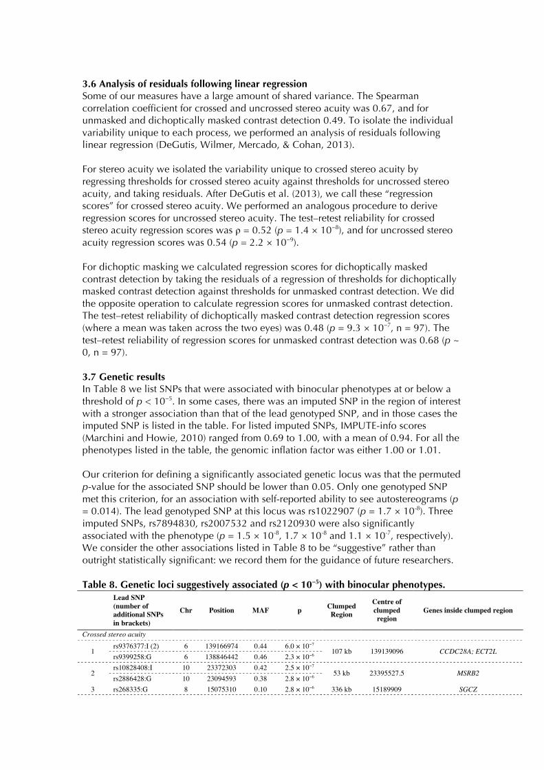
3.6 Analysis of residuals following linear regression Some of our measures have a large amount of shared variance. The Spearman correlation coefficient for crossed and uncrossed stereo acuity was 0.67, and for unmasked and dichoptically masked contrast detection 0.49. To isolate the individual variability unique to each process, we performed an analysis of residuals following linear regression (DeGutis, Wilmer, Mercado, & Cohan, 2013). For stereo acuity we isolated the variability unique to crossed stereo acuity by regressing thresholds for crossed stereo acuity against thresholds for uncrossed stereo acuity, and taking residuals. After DeGutis et al. (2013), we call these “regression scores” for crossed stereo acuity. We performed an analogous procedure to derive regression scores for uncrossed stereo acuity. The test–retest reliability for crossed stereo acuity regression scores was ρ = 0.52 (p = 1.4 × 10⁻⁸), and for uncrossed stereo acuity regression scores was 0.54 (p = 2.2 × 10⁻⁹). For dichoptic masking we calculated regression scores for dichoptically masked contrast detection by taking the residuals of a regression of thresholds for dichoptically masked contrast detection against thresholds for unmasked contrast detection. We did the opposite operation to calculate regression scores for unmasked contrast detection. The test–retest reliability of dichoptically masked contrast detection regression scores (where a mean was taken across the two eyes) was 0.48 (p = 9.3 × 10⁻⁷, n = 97). The test–retest reliability of regression scores for unmasked contrast detection was 0.68 (p ~ 0, n = 97). 3.7 Genetic results In Table 8 we list SNPs that were associated with binocular phenotypes at or below a threshold of p < 10−5. In some cases, there was an imputed SNP in the region of interest with a stronger association than that of the lead genotyped SNP, and in those cases the imputed SNP is listed in the table. For listed imputed SNPs, IMPUTE-info scores (Marchini and Howie, 2010) ranged from 0.69 to 1.00, with a mean of 0.94. For all the phenotypes listed in the table, the genomic inflation factor was either 1.00 or 1.01. Our criterion for defining a significantly associated genetic locus was that the permuted p-value for the associated SNP should be lower than 0.05. Only one genotyped SNP met this criterion, for an association with self-reported ability to see autostereograms (p = 0.014). The lead genotyped SNP at this locus was rs1022907 (p = 1.7 × 10⁻⁸). Three imputed SNPs, rs7894830, rs2007532 and rs2120930 were also significantly associated with the phenotype (p = 1.5 × 10⁻⁸, 1.7 × 10⁻⁸ and 1.1 × 10⁻⁷, respectively). We consider the other associations listed in Table 8 to be “suggestive” rather than outright statistically significant: we record them for the guidance of future researchers. Table 8. Genetic loci suggestively associated (p < 10−5) with binocular phenotypes.
Lead SNP (number of additional SNPs in brackets)
Chr Position MAF p Clumped Region
Centre of clumped region
Genes inside clumped region
Crossed stereo acuity
1 rs9376377:I (2) 6 139166974 0.44 6.0 × 10⁻⁷
107 kb 139139096 CCDC28A; ECT2L rs9399258:G 6 138846442 0.46 2.3 × 10⁻⁶
2 rs10828408:I 10 23372303 0.42 2.5 × 10⁻⁷
53 kb 23395527.5 MSRB2 rs2886428:G 10 23094593 0.38 2.8 × 10⁻⁶
3 rs268335:G 8 15075310 0.10 2.8 × 10⁻⁶ 336 kb 15189909 SGCZ

4 rs12465282:G 2 36619764 0.36 3.2 × 10⁻⁶ 157 kb 36653372.5 CRIM1 5 rs4702797:G 5 11286173 0.11 5.2 × 10⁻⁶ 25 kb 11273646 CTNND2 6 rs4491324:G 12 4082865 0.41 7.4 × 10⁻⁶ 10 kb 4083284 N/A
7 rs8115802:I (1) 20 13857593 0.47 6.6 × 10⁻⁶
336 kb 13858987.5 ESF1; NDUFAF5; SEL1L2; MACROD2 rs6134980:G 20 13833963 0.35 8.0 × 10⁻⁶
8 rs11036885:G 11 5357048 0.07 8.8 × 10⁻⁶ 138 kb 5400722.5 HBE1; OR51B2; OR51B5;
OR51B6; OR51M1; OR51Q1; OR51I1
Uncrossed stereo acuity
9 rs7470783:I (75) 9 83532189 0.07 1.5 × 10⁻⁸
311 kb 83556498 N/A rs17245550:G (1) 9 80972511 0.07 2.2 × 10⁻⁶
10 rs7048502:I (1) 9 3711623 0.03 5.4 × 10⁻⁶
31 kb 2052398.5 N/A rs7871296:G 9 3710068 0.03 6.2 × 10⁻⁶
11 rs35582814:I (1) 20 57440586 0.15 4.3 × 10⁻⁶
140 kb 57384667 GNAS−AS1; GNAS rs8125112:G 20 58856110 0.15 8.4 × 10⁻⁶
Average stereo acuitya
12 rs35600882:I (17) 3 174747248 0.17 1.8 × 10⁻⁷
114 kb 174741283 NAALADL2 rs11928561:G 3 175073529 0.11 5.7 × 10⁻⁶
TNO stereo acuity (rank)
14 rs4533756:G 4 25062976 0.04 7.0 × 10⁻⁶ 7 kb 25062757.5 N/A
Binocular rivalry median percept duration
15 rs6535700:I 4 49981463 0.25 3.2 × 10⁻⁶
266 kb 150820285 N/A rs3923657:G 4 149997646 0.28 6.5 × 10⁻⁶
16
rs117479286:I 20 45970648 0.03 4.4 × 10⁻⁶
212 kb 44550013.5
UBE2C; TNNC2; SNX21; ACOT8; ZSWIM3; ZSWIM1; SPATA25; NEURL2; CTSA;
PLTP; PCIF1; ZNF335; MMP9; SLC12A5
rs3746513:G 20 45965589 0.35 8.2 × 10⁻⁶
Binocular rivalry standard deviation of percept duration
17 rs6442155:I (1) 3 130670 0.20 3.5 × 10⁻⁷
313 kb 43506666.5 SNRK; ANO10 rs9832112:G (1) 3 129625 0.20 5.7 × 10⁻⁷
18 rs12421008:I 11 34627093 0.04 5.9 × 10⁻⁷
32 kb 34637627 EHF rs11032786:G (1) 11 34618757 0.08 9.6 × 10⁻⁷
19 rs72912297:I (83) 7 56219962 0.17 5.5 × 10⁻⁷
1330 kb 56438519.5 SEPT14; ZNF713; MRPS17;
GBAS; PSPH; SUMF2; CCT6A; PHKG1; CHCHD2; NUPR1L rs10499761:G (1) 7 56125950 0.17 3.2 × 10⁻⁶
20 rs17155559:G 5 102946979 0.09 8.5 × 10⁻⁶ 56 kb 102952551.5 N/A 21 rs1956451:G 14 94620193 0.14 8.7 × 10⁻⁶ 178 kb 94672512 IFI27L2; PPP4R4; SERP1NA10
Log unmasked contrast threshold
22 rs1894657:I (1) 22 45522232 0.47 1.3 × 10⁻⁷
26 kb 252591065 FBLN1 rs2018072:G 22 45522611 0.47 5.2 × 10⁻⁷
23 rs75587525:I (1) 9 1311440 0.03 9.7 × 10⁻⁷
33 kb 1302070 N/A rs16927344:G 9 1311310 0.03 2.3 × 10⁻⁶
24 rs871664:G 1 94609478 0.47 4.9 × 10⁻⁶ 270 kb 94721365 ABCA4; ARHGAP29
25 rs11102983:I (1) 1 109434985 0.04 2.0 × 10⁻⁶
254 kb 109951198 PSRC1; MYBPHL; SORT1;
PSMA5; SYPL2; CYB561D1; AMIGO1 rs629001:G 1 109296296 0.07 6.5 × 10⁻⁶
26 rs67102156:I (3) 10 36623082 0.07 5.9 × 10⁻⁶
157 kb 36553598.5 N/A rs7913838:G 10 36310294 0.07 7.2 × 10⁻⁶
27 rs28410795:I 4 178770987 0.43 4.9 × 10⁻⁶
108 kb 179658484 N/A rs1947202:G 4 178784154 0.42 9.0 × 10⁻⁶
28 rs9823729:I 3 178256533 0.50 6.7 × 10⁻⁶
232 kb 177983588.5 N/A rs6808802:G 3 178252979 0.50 9.3 × 10⁻⁶
Log masked contrast threshold
29 rs28844067:I (2) 16 54665636 0.49 2.9 × 10⁻⁸ 54 kb 54712214 N/A

rs11639521:G 16 54675298 0.49 9.4 × 10⁻⁸ 30 rs12904615:G 15 85549722 0.48 3.5 × 10⁻⁶ 604 kb 85820420.5 PDE8A; AKAP13
31 rs6566439:I (6) 18 69704564 0.31 5.3 × 10⁻⁶
63 kb 67368313 DOK6 rs4393673:G 18 69721118 0.30 8.8 × 10⁻⁶
32 rs6427351:G 1 157066950 0.09 8.8 × 10⁻⁶ 8 kb 157070368.5 ETV3L
33 rs8106814:I 19 44938351 0.27 2.6 × 10⁻⁶
73 kb 45477307.5 APOC4−APOC2; CLPTM1; RELB rs10413089:G 19 44952331 0.18 9.5 × 10⁻⁶
Ability to see autostereograms
34 rs7894830:I 10 114394794 0.34 1.5 × 10⁻⁸
58 kb 114419076.5 VTI1A rs1022907:G 10 112635088 0.35 1.7 × 10⁻⁸
Statistics are based on a quantitative trait analysis, using ranked data for each phenotype and 4 covariates (sex and the first 3 genetic PCAs).
Following the SNP identifier is ‘G’ for a genotyped SNP and ‘I’ for an imputed SNP. Imputed SNPs are listed only if the p-value of the association is smaller than that for the most strongly
associated genotyped SNP at the same locus. At some loci more than one SNP was suggestively associated with the phenotype. The number of additional associated SNPs at a given locus is
given in brackets after the SNP identifier. a rs17245550, rs268335, rs7871296, rs10491944, rs4702797 (6.9 × 10⁻⁶ ≥ p ≥ 1.7 × 10⁻⁶)
emerged as suggestive associations for mean stereo acuity but are listed under either crossed or uncrossed stereo acuity.
4.0 Discussion 4.1 Stereo acuity Median stereo acuity for our sample of 1060 participants was 60 seconds of arc for the TNO test and 88.2 seconds of arc for our adaptive test (averaged over measurements for crossed and uncrossed stereo acuity). These median values are larger than those reported in the few other population studies of stereo acuity in adults that we have found, where estimates range from 12.4 to 37.2 seconds of arc (Bohr & Read, 2013; Coutant & Westheimer, 1993; Zaroff, 2003). These differences could be caused by variety of tasks, variety of population samples, or practice effects. In particular, in our adaptive test the stimuli were presented at an eccentricity of 0.7°. We can assess the impact of perceptual learning on stereo thresholds by comparing the performance of our 105 returning participants in the first and second sessions: There was in fact no significant difference between stereo thresholds measured in the first and second sessions (t = 0.4, p = 0.69 for crossed stereo acuity; t = −0.14, p = 0.89 for uncrossed stereo acuity; t = −1.5, p =0.13 for the TNO). Although differences in perceptual learning may contribute to the variability in median stereo thresholds found across studies, but we have found no evidence that it affects performance on our tasks. We found that 8.9% of participants performed at ceiling on the TNO test (480 arc seconds), 10.4% performed at ceiling on our adaptive test for crossed stereo acuity (350 arc seconds), 9.2% performed at ceiling on our adaptive test for uncrossed stereo acuity (350 arc seconds). However, only 5.3% of participants performed at ceiling on both adaptive tests, and only 2.2% of participants performed at ceiling on both adaptive tests and on the TNO test. Thus, in 2.2% of our participants, we could find no evidence of stereopsis. Our results may help to explain why estimates of stereo blindness from population studies have varied widely from 1 to 14% (Bohr & Read, 2013; Coutant & Westheimer, 1993; Rahi et al., 2009; W Richards, 1970; Zaroff, 2003). It may be that particular individuals have particular difficulties with certain tests of stereo acuity. The TNO test was personally administered by experimenters, and we found that some participants

needed encouragement to “tune in” to the disparity information—but once they had, their thresholds could be quite low. (“Tuning in” may be the process of learning to attend to the relevant signal, as proposed by Mollon and Danilova (1996).) For our adaptive test an example stimulus was presented as part of the instructions, and participants called the experimenter if they could not perceive the depth. Again, some participants suddenly perceived depth once their attention was drawn to it. Naïve psychophysical subjects are unlikely to be practised at perceiving disparity information in the absence of other depth cues. They may need time and encouragement to attend to the relevant signal; and, since we have found that individuals can perform at ceiling on some stereo tasks and not others, learning to attend to the relevant signal may not transfer fully between different stereo tasks. 4.1.2 Crossed and uncrossed stereo acuity There is divided opinion over whether crossed and uncrossed stereopsis are subserved by different mechanisms. Whitman Richards proposed not only that crossed and uncrossed stereopsis rely on different neural machinery (Richards, 1971; Richards & Regan, 1973), but that the inheritance of each ability can be described by a simple genetic model (Richards, 1970). In our population, crossed and uncrossed stereo acuities measured using our adaptive test are highly correlated (ρ = 0.67). However, both crossed and uncrossed stereo acuity show significant test–retest reliability when the effect of the other is regressed out (ρ = 0.52 for crossed stereo acuity, and ρ = 0.54 for uncrossed stereo acuity). The correlation between crossed and uncrossed stereo acuity is greater than the reliabilities of the residuals for each ability following regression on the other. But does this imply that the amount of variance shared between crossed and uncrossed stereo acuity is greater than the amount of variance unique to each? The direct comparison neglects the fact that the correlation between measures (over the whole sample of 1060 participants) is within-session, while test–retest reliabilities use data gathered over two independent sessions (from our 105 returning participants). Using data gathered in different sessions will add additional sources of variability. In order to make a fair comparison, we can use inter-test reliabilities (Goodbourn et al., 2012), where performance on one measure gathered in session 1 is correlated with performance on a different measure gathered in session 2, and vice versa. The inter-test reliabilities for crossed and uncrossed stereo acuity are ρ = 0.61 (p = 3.6 x10⁻¹²) and ρ = 0.58 (p = 1.3x10⁻¹⁰). A comparison of inter-test reliabilities (0.61 and 0.58) and the reliabilities of the regression scores (0.52 and 0.54) shows that the proportion of variance shared between crossed and uncrossed stereo acuity tends to be somewhat greater than the proportion of variance unique to either measure. However, the difference between the correlation coefficients is not significant. The shared variance between thresholds for crossed and uncrossed stereo disparities implies that a common mechanism subserves part of the individual variation in crossed and uncrossed stereo acuity. Similarly, the significant test-retest reliabilities of the regression scores shows that part of the individual variation in stereo acuity derives from mechanisms unique to crossed and to uncrossed disparities. 4.2 Correlations between measures We have found significant correlations within our set of binocular measures, as well as between the binocular measures and demographic and anatomical measures, and with other psychophysical measures. Some measures we included in the battery to confirm associations already reported in the literature, and we have replicated these findings in our large sample, though typically with a smaller effect size.

The correlation we might expect to be strongest is between the two measures of stereo acuity, our adaptive test and the TNO test. Yet this correlation is only moderate at ρ = 0.32. Noise in both measures—suggested by the test–retest reliabilities—means that even if the variables were truly perfectly correlated, we would expect to observe a correlation coefficient of only 0.44. Taking the test-retest reliabilities into account, we can estimate the correlation between the “universe scores” (the mean of an infinite number of measurements) as 0.72. The effect sizes of other significant correlations that we have found must also be interpreted with the limits imposed by measurement noise in mind. We have found that stereo acuity is significantly correlated with binocular visual acuity. It is also separately significantly correlated with visual acuity in both the better and the worse eye, though the correlation is stronger with visual acuity in the worse eye. Stereo acuity correlates more strongly still with interocular difference in visual acuity. We found one correlational study for individual differences in visual acuity and individual differences in stereo acuity: Lam et al. (1996) report a negative correlation between interocular difference in visual acuity and stereo acuity. Our results are in concordance with their finding. There are a number of reports that stereo acuity worsens when visual acuity is disrupted using lenses (Costa, Moreira, Hamer, & Ventura, 2010; Goodwin & Romano, 1985; Odell, Hatt, Leske, Adams, & Holmes, 2009), or anisometropia is artificially induced (Brooks, Johnson, & Fischer, 1996; Oguz & Oguz, 2000). Replicating Baker and Graf (2009), we find a significant relationship between the magnitude of dichoptic masking and the rate of binocular rivalry, with stronger masking associated with longer percept durations. We also replicated Wilmer and Backus’ (2008) finding that stereo acuity is positively associated with self-reported ability to see autostereograms. Our finding that rate of binocular rivalry decreases with age replicates earlier reports by Jalavisto (1964) and Ukai et al. (2003). However, these earlier studies included older participants (40–80+ for Jalavisto and 20–64 for Ukai et al.) than did the present study, where ages were restricted from 16 to 40. Our finding of the relationship in young subjects suggests that declining rivalry rates are not caused by optical effects of aging. Indeed, when visual acuity with usual correction is entered as a covariate into the correlation, its size barely changes (ρ = 0.14, p = 4.8 × 10⁻⁶). In unmasked contrast detection, we found a significant sex difference: Men, on average, were 0.3 standard deviations more sensitive than women. Where sex differences in contrast sensitivity have been reported in the literature, they tend to be in the same direction as in the present study (Abramov, Gordon, Feldman, & Chavarga, 2012; Hashemi et al., 2012; Oen, Lim, & Chung, 1994). Brabyn and McGuinness (1979) report an interaction between sex and spatial frequency with females superior at low spatial frequencies and males at high. In other cases no significant sex differences have been found (Owsley, Sekuler, & Siemsen, 1983; Solberg & Brown, 2002). We note that a sample size of 330 would be needed to detect with 80% power an effect of the size that we found in the present study, and that typical past sample sizes have been much smaller than this. However, we must interpret our sex difference with caution because we have not randomly sampled total male and female populations.

Surprisingly, we found only a small correlation (ρ = 0.07) of inter-pupillary distance (IPD) with stereo acuity measured using the TNO test, and no significant correlation with stereo acuity measured using our adaptive test. The correlation between IPD and TNO score was positive, meaning stereo acuity tends to be worse with greater IPD. But what relationship should we expect? In the real world, a greater IPD means greater binocular disparities, and presumably superior ability to detect small differences in depth. But in tests of stereo acuity the binocular disparities are fixed. A given disparity would correspond to smaller differences in real-world depth for someone with a small IPD than for someone with a large IPD. We should therefore expect that performance on these tests would not improve and might even worsen with increasing IPD. Our largely negative finding is supported by previous studies (Eom et al., 2013). Frisby et al. (2003) report a positive correlation between IPD and stereo acuity using the real-depth Howard-Dolman test, as would be expected. We found no significant differences in unmasked or binocularly masked contrast thresholds between the sighting dominant and the non-dominant eyes. This may seem surprising, but is consistent with previous findings that there is no correlation between sighting dominance and “sensory” dominance, defined by best visual performance, for example best acuity, or best contrast sensitivity (Mapp, Ono, & Barbeito, 2003; Porac & Coren, 1975; Suttle et al., 2009). We did find that for binocular rivalry, the stimulus presented to the dominant eye is perceived for a significantly greater proportion of the time than the stimulus presented to the non-dominant eye. This is consistent with earlier results (Handa et al., 2004; Porac & Coren, 1978). Perhaps surprisingly, we found no strong correlations between stereo acuity and phorias, whether phorias were scaled from esophoria to exophoria or were expressed absolutely. The relationship between stereo acuity and phorias has also been investigated in several earlier studies. Lam et al. (2002) also found no significant correlation between phoria and either crossed or uncrossed stereo acuity, but found that in exophores only, crossed stereo acuity was superior to uncrossed stereo acuity. Shippman and Cohen (1983) found that exophores have better crossed than uncrossed stereo acuity while esophores show the opposite pattern. When we break down the data from our adaptive test in the same way, defining exophoria and esophoria (following Lam et al.) as deviations greater than 2 diopters, we find the same pattern as Shippman and Cohen. For near phoria, orthophores show no significant difference between crossed and uncrossed stereo acuity ( crossed = 118.3, uncrossed = 118.8, t = 0.09, p = 0.92), exophores show significantly better crossed than uncrossed stereo acuity ( crossed = 121.7, uncrossed = 128.6, t = 2.29, p = 0.02) and esophores show significantly better uncrossed than crossed stereo acuity ( crossed = 152.7, uncrossed = 135.1, t = 2.25, p = 0.03). This small—though interesting—difference between the groups may result, as Shippman and Cohen suggest, from different asymmetries in Panum’s area between groups. Saladin (1995) found in a large population that stereo acuity worsened with increasing esophoria but was not significantly affected by exophoria. Though our correlations between stereo acuity and phoria are small, there may be non-linear relationships like those found by Saladin. Figure 3 is the equivalent of Saladin’s Figure 1, except that we include crossed and uncrossed stereo acuity, and near and far horizontal phorias, separately. The figure shows a negative linear relationship between crossed stereo acuity and far phoria. For crossed stereo acuity, as Saladin found, esophores are impaired but exophores are not. For uncrossed acuity the relationship with near (but

not far) phorias is U-shaped, with both esophores and exophores impaired relative to orthophores.
Figure 3. Relationship between near and far horizontal phorias and crossed and uncrossed stereo acuity. Data points are omitted where N ≤ 2. We found a number of correlations between binocular performance measures and other psychophysical measures included in the PERGENIC test battery (see Table 7), with effect sizes ranging up to r2 = 0.14. The strongest correlations were between masked and unmasked contrast detection on the one hand, and detection of coherent form and gratings of low spatial frequency on the other. These probably reflect a general ability of contrast sensitivity. There were also substantial correlations between stereo acuity and thresholds for detecting coherent form, but not between stereo acuity and thresholds for detecting gratings of low spatial frequency. Perhaps the strong correlation between stereo acuity and thresholds for coherent form arises because both tasks depend on orientationally selective detectors. More unexpected are correlations with thresholds for coherent motion (r2= 0.04 for stereo acuity and r2= 0.08 for masked contrast detection).
−10 −5 0 5 10 15 2060
80
100
120
140
160
180
200
220
−10 −5 0 5 10 15 2060
80
100
120
140
160
180
200
220Near phoria Far phoria
crosseduncrossed
crosseduncrossed
phoria phoria
ster
eo a
cuity
(s
econ
ds o
f arc
)
exophoriaesophoria exophoriaesophoria
0
20
40
Rec
ombi
natio
n ra
te (c
M/M
b)
0
2
4
6
8
−log 10(p)
Chromosome 10 position (kb)113600 114400 115200
GPAM
TECTB
ACSL5
ZDHHC6
VTI1A
TCF7L2 HABP2
NRAP
CASP7
PLEKHS1
DCLRE1A
NHLRC2
a1 2 3 4 5
a
0
200
400
Likert scale
n
(a)
(b)
(c)

Figure 4. Regional Manhattan diagram for the association between self-reported ability to see autostereograms and the region around rs1022907. Panel (a) shows the distribution of the phenotype, which was agreement with the questionnaire item “I am good at seeing Magic Eye puzzles (stereograms),” on a Likert scale of 1-5. Panel (b) shows association results. Results for genotyped SNPs are drawn with black borders, and results for imputed SNPs are drawn without borders. Saturation is scaled with IMPUTE-info score. The recombination rate is plotted in blue. Panel (c) shows the positions of genes in the region. Exons are indicated by the vertical green lines, and transcription direction by the green arrows. The dashed vertical blue lines in panels (b) and (c) enclose the region of interest identified by clumping analysis. Table 9. Genes in suggestively associated regions that have been associated with brain or eye development and function Brain or eye development CRIM1 Neural morphogenesis Kolle, Georgas, Holmes, Little, & Yamada (2000); Ponferrada et al., (2012)
Retinal vascular stability during development Fan et al. (2014) CTNND2 Regulation of spine and synapse morphogenesis Arikkath et al. (2009) SEPT14 Cortical neuronal migration Shinoda et al. (2010) AMIGO1 Promotes growth and fasciculation of neurites Chen, Hor, & Tang (2012); Kuja-Panula, Kiiltomäki, Yamashiro,
Rouhiainen, & Rauvala, (2003) DOK6 Promotes RET-mediated neurite growth Crowder, Enomoto, Yang, Johnson, & Milbrandt (2004) SLC12A5 Terminates GABA-mediated cortical migration of
Interneurons in the developing brain Bortone & Polleux (2009)
ETV3L Inhibits the action of ETS genes in mediating primary neurogenesis
Janesick et al. (2013)
Brain or eye function CTNND2 Activity dependent synaptic plasticity Brigidi et al. (2014)
Maintenance of dendrites in mature cortex Matter, Pribadi, Liu, & Trachtenberg (2009) SLC12A5 Encodes KCC2, the main K-Cl transporter to
extrude choride for promotion of fast hyperpolarising postsynaptic inhibition in the brain
Rivera et al. (1999)
CRIM1 Candidate gene for plasticity in ocular dominance columns
Rietman, Sommeijer, Levelt, & Heimel (2012)
ABCA4 Encodes an ATP-binding cassette transporter that clears all-trans-retinal aldehyde from photoreceptors
Sun et al. (1999)
Brain or eye pathologies NDUFAF5 Leigh syndrome Benit et al. (2004); Finsterer, (2008) CTNND2 Pathological myopia Li et al. (2011); Liu & Zhang (2014); Lu et al. (2011); Yu et al. (2012)
Cri du Chat syndrome Medina, Marinescu, Overhauser, & Kosik (2000) Age-related cataract Jun et al. (2012)
MACROD2 Autism Anney et al. (2010) ADHD Lionel et al. (2011)
SLC12A5 Schizophrenia Tao et al. (2012) ANO10 Spinocerebellar ataxia Chamova et al. (2012); Vermeer et al. (2010) FBLN1 In a chromosomal section, containing four genes,
that has been associated with vitreoretinal dystrophy Weigell-Weber et al. (2003)
ABCA4 Rod-cone dystrophy Kitiratschky et al. (2008); Maugeri et al. (2000) Fundus flavimaculatus Allikmets et al. (1997); Azarian & Travis (1997); Illing, Molday, & Molday,
(1997) Age-related macular degeneration Fritsche et al. (2012)
4.3 Genetics Because our sample of 988 was small by the standards of GWAS, all our associations, including between rs1022907 and self-reported ability to see autostereograms (p = 1.7 × 10⁻⁸) must be considered preliminary. We list the suggestive associations here as a resource for future researchers, to be independently replicated. Future studies should take account of the fact that the effect sizes of true positives are likely to be inflated by the winner’s curse (Lohmueller et al., 2003; Xiao and Boehnke, 2011), What we can conclude, by the absence of very large genetic associations, is that the individual variability in binocular traits that we have measured in our sample is unlikely to be

monogenic or oligogenic. Instead, the putative genetic determinants of performance on our binocular tasks may be many and varied, with a large number of loci each contributing a small effect. The association between rs1022907 and self-reported ability to see autostereograms was the only association to pass the stringent permutation test (p = 0.014). Since the correlations between self-reported ability to see autostereograms and our psychophysical measures of stereo acuity are fairly low (ρ = 0.14 for TNO and ρ = 0.16 for our adaptive test), the association may not be due to individual differences in stereo acuity. Indeed, when TNO score and score on our adaptive measure of stereo acuity are introduced into the association as covariates, the p-value of the association increases only slightly to 8.8 × 10⁻⁸. A Manhattan diagram for the region around rs1022907 is shown in Figure 4. The associated SNP, rs1022907, lies in an intronic region of the gene VTI1A, which encodes the v-SNARE protein VTI1A. The associated region of interest surrounding rs1022907 also contains the 6th and 7th exons of VTI1A, and the microRNA MIR4295. Two functions of VTI1A may be relevant to the genetic association we find here: It selectively maintains spontaneous (rather than evoked) neurotransmitter release (Ramirez, Khvotchev, Trauterman, & Kavalali, 2012), and it is involved in the development of neurons and axon tracts (Kunwar et al., 2011). Specifically relevant to binocular vision is the finding that in mice double knockout for VTI1A and VTI1B, the optic tract and optic chiasm are diminished. If the association between rs1022907 and self-reported ability to see autostereograms is not driven by individual differences in stereo acuity, what might be driving it? We correlated response on the autostereogram questionnaire item with performance on many other psychophysical and questionnaire measures gathered for PERGENIC. Apart from correlations with stereo acuity, there were significant positive correlations (α = 0.0003, after correction for 169 comparisons) with other self-reported abilities including aptitude for sport and ball sports, and self-reported synesthesia; and there were negative correlations with several measures of mean response time and variability of response times in psychophysical tasks. However, with none of these measures was associated with rs1022907, even at p < 0.05. There are 33 additional loci, containing 68 genes, suggestively associated with binocular traits (see Table 8). Of these, genes that have been implicated previously in brain or eye development, brain function in adults, or brain and eye pathologies may be the most plausible candidates. We summarise existing findings about these candidates in Table 9. An interesting pair are ETV3L and EHF: ETV3L is a retinoic acid target gene that inhibits the action of ETS genes (of which EHF is a member) in mediating primary neurogenesis (Janesick et al., 2013). Two genes (CLPTM1 and ARHGAP29) are associated with cleft lip and palette (Beaty et al., 2010; Leslie et al., 2013; Yoshiura et al., 1998); it may be relevant that there are ocular abnormalities in some patients (Anchlia, Rao, Bonanthaya, Anupama, & Nayak, 2011). ABCA4 is a very plausible candidate for contrast sensitivity: This gene encodes an ATP-binding cassette transporter that is expressed exclusively in retinal photoreceptor cells

and that clears all-trans-retinal aldehyde. It is associated with rod-cone dystrophy (Kitiratschky et al., 2008; Maugeri et al., 2000), fundus flavimaculatus (Allikmets et al., 1997; Azarian & Travis, 1997; Illing, Molday, & Molday, 1997) and age-related macular degeneration (Fritsche et al., 2012). Acknowledgements This work was supported by the Gatsby Charitable Foundation (GAT2903). J.B. was supported by a fellowship from Gonville and Caius College. The authors are grateful to Horace Barlow, Roger Freedman, Graeme Mitchison and Richard Durbin for their role in the initiation of the PERGENIC project, and to Emily Clemente, Julien Bauer, and Kerry Cliffe of Cambridge Genomic Services for their valuable help.
References Abecasis, G. R., Altshuler, D., Auton, A., Brooks, L. D., Durbin, R. M., Gibbs, R. A., … McVean, G. A. (2010). A
map of human genome variation from population-‐scale sequencing. Nature, 467(7319), 1061–1073. doi:10.1038/nature09534
Abramov, I., Gordon, J., Feldman, O., & Chavarga, A. (2012). Sex & vision I: Spatio-‐temporal resolution. Biology of Sex Differences, 3(1), 20.
Allikmets, R., Singh, N., Sun, H., Shroyer, N., Hutchinson, A., Chidambaram, A., … Lupski, J. (1997). A photoreceptor cell-‐specific ATP-‐binding transporter gene (ABCR) is mutated in recessive Stargardt macular dystrophy. Nature Genetics, 15, 236–246.
Anchlia, S., Rao, K. S., Bonanthaya, K., Anupama, B., & Nayak, I. V. (2011). Ophthalmic considerations in cleft lip and palate patients. Journal of Maxillofacial and Oral Surgery, 10(1), 14–19.
Anney, R., Klei, L., Pinto, D., Regan, R., Conroy, J., Magalhaes, T. R., … Hallmayer, J. (2010). A genome-‐wide scan for common alleles affecting risk for autism. Human Molecular Genetics, 19(20), 4072–4082.
Arikkath, J., Peng, I.-‐F., Ng, Y. G., Israely, I., Liu, X., Ullian, E. M., & Reichardt, L. F. (2009). Delta-‐catenin regulates spine and synapse morphogenesis and function in hippocampal neurons during development. The Journal of Neuroscience, 29(17), 5435–5442.
Azarian, S. M., & Travis, G. H. (1997). The photoreceptor rim protein is an ABC transporter encoded by the gene for recessive Stargardt’s disease (ABCR). FEBS Letters, 409(2), 247–252.
Baker, D. H., & Graf, E. W. (2009). On the relation between dichoptic masking and binocular rivalry. Vision Research, 49(4), 451–459.
Baker, D. H., & Meese, T. S. (2007). Binocular contrast interactions: dichoptic masking is not a single process. Vision Research, 47(24), 3096–3107.
Barlow, H. B., Blakemore, C., & Pettigrew, J. D. (1967). The neural mechanism of binocular depth discrimination. The Journal of Physiology, 193, 327–342.
Baron-‐Cohen, S., Wheelwright, S., Skinner, R., Martin, J., & Clubley, E. (2001). The autism-‐spectrum quotient (AQ): evidence from Asperger syndrome/high-‐functioning autism, males and females, scientists and mathematicians. Journal of Autism and Developmental Disorders, 31(1), 5–17.
Barry, S. R. (2012). Beyond the Critical Period: Acquiring Stereopsis in Adulthood. In J. K. E. Steeves & L. R. Harris (Eds.), Plasticity in Sensory Systems (pp. 175–195). Cambridge, UK: Cambridge University Press.
Beaty, T. H., Murray, J. C., Marazita, M. L., Munger, R. G., Ruczinski, I., Hetmanski, J. B., … Scott, A. F. (2010). A genome-‐wide association study of cleft lip with and without cleft palate identifies risk variants near MAFB and ABCA4. Nature Genetics, 42(6), 525–529.
Bénit, P., Slama, A., Cartault, F., Giurgea, I., Chretien, D., Lebon, S., … Rustin, P. (2004). Mutant NDUFS3 subunit of mitochondrial complex I causes Leigh syndrome. Journal of Medical Genetics, 41(1), 14–17.
Birch, E. E., Gwiazda, J., & Held, R. (1982). Stereoacuity development for crossed and uncrossed disparities in human infants. Vision Research, 22, 507–513.
Blakemore, C. (1979). The Development of Stereoscopic Mechanisms in the Visual Cortex of the Cat. Proceedings of the Royal Society B: Biological Sciences, 204(1157), 477–484.
Bohr, I., & Read, J. C. (2013). Stereoacuity with Frisby and revised FD2 stereo tests. PloS One, 8(12), e82999. Bortone, D., & Polleux, F. (2009). KCC2 expression promotes the termination of cortical interneuron
migration in a voltage-‐sensitive calcium-‐dependent manner. Neuron, 62(1), 53–71. Bosten, J. M., Bargary, G., Goodbourn, P. T., Hogg, R. E., Lawrance-‐Owen, A. J., & Mollon, J. D. (2014).
Individual differences provide psychophysical evidence for separate on-‐ and off-‐pathways deriving from short-‐wave cones. Journal of the Optical Society of America. A, 31(4), A47–A54.
Bosten, J. M., Hogg, R. E., Bargary, G., Goodbourn, P. T., Lawrance-‐Owen, A. J., & Mollon, J. D. (2014). Suggestive association with ocular phoria at chromosome 6p22. Investigative Ophthalmology & Visual Science, 55(1), 345–352.
Brabyn, L. B., & McGuinness, D. (1979). Gender differences in response to spatial frequency and stimulus orientation. Perception & Psychophysics, 26(4), 319–324.

Brainard, D. H. (1997). The Psychophysics Toolbox. Spatial Vision, 10(4), 433–436. Brigidi, G. S., Sun, Y., Beccano-‐Kelly, D., Pitman, K., Mobasser, M., Borgland, S. L., … Bamji, S. X. (2014).
Palmitoylation of δ-‐catenin by DHHC5 mediates activity-‐induced synapse plasticity. Nature Neuroscience, 17(4), 522–532.
Brooks, S. E., Johnson, D., & Fischer, N. (1996). Anisometropia and binocularity. Ophthalmology, 103(7), 1139–1143.
Chamova, T., Florez, L., Guergueltcheva, V., Raycheva, M., Kaneva, R., Lochmüller, H., … Tournev, I. (2012). ANO10 c.1150_1151del is a founder mutation causing autosomal recessive cerebellar ataxia in Roma/Gypsies. Journal of Neurology, 259(5), 906–911.
Chen, Y., Hor, H. H., & Tang, B. L. (2012). AMIGO is expressed in multiple brain cell types and may regulate dendritic growth and neuronal survival. Journal of Cellular Physiology, 227(5), 2217–2229.
Costa, M. F., Moreira, S. M., Hamer, R. D., & Ventura, D. F. (2010). Effects of age and optical blur on real depth stereoacuity. Ophthalmic & Physiological Optics, 30(5), 660–666.
Coutant, B. E., & Westheimer, G. (1993). Population distribution of stereoscopic ability. Ophthalmic & Physiological Optics, 13(1), 3–7.
Crowder, R. J., Enomoto, H., Yang, M., Johnson, E. M., & Milbrandt, J. (2004). Dok-‐6, a Novel p62 Dok family member, promotes Ret-‐mediated neurite outgrowth. The Journal of Biological Chemistry, 279(40), 42072–42081.
DeGutis, J., Wilmer, J., Mercado, R. J., & Cohan, S. (2013). Using regression to measure holistic face processing reveals a strong link with face recognition ability. Cognition, 126(1), 87–100.
Donnellan, M., Oswald, F. L., Baird, B. M., & Lucas, R. E. (2006). The mini-‐IPIP scales: tiny-‐yet-‐effective measures of the Big Five factors of personality. Psychological Assessment, 18(2), 192–203.
Eom, Y., Song, J.-‐S., Ahn, S.-‐E., Kang, S.-‐Y., Suh, Y.-‐W., Oh, J., … Kim, H. M. (2013). Effects of interpupillary distance on stereoacuity: the Frisby Davis distance stereotest versus a 3-‐dimensional distance stereotest. Japanese Journal of Ophthalmology, 57(5), 486–492.
Fan, J., Ponferrada, V. G., Sato, T., Vemaraju, S., Fruttiger, M., Gerhardt, H., … Lang, R. A. (2014). Crim1 maintains retinal vascular stability during development by regulating endothelial cell Vegfa autocrine signaling. Development, 141(2), 448–459.
Finsterer, J. (2008). Leigh and Leigh-‐like syndrome in children and adults. Pediatric Neurology, 39(4), 223–235.
Frisby, J., Davis, H., & Edgar, R. (2003). Does interpupillary distance predict stereoacuity for normal observers? Perception, 32(ECVP Abstract Supplement) 73–74.
Fritsche, L. G., Fleckenstein, M., Fiebig, B. S., Schmitz-‐Valckenberg, S., Bindewald-‐Wittich, A., Keilhauer, C. N., … Weber, B. H. (2012). A subgroup of age-‐related macular degeneration is associated with mono-‐allelic sequence variants in the ABCA4 gene. Investigative Ophthalmology & Visual Science, 53(4), 2112–2118.
Glass, L. (1969). Moiré Effect from Random Dots. Nature, 223, 578–580. Goodbourn, P. T., Bosten, J. M., Bargary, G., Hogg, R. E., Lawrance-‐Owen, A. J., & Mollon, J. D. (2014). Variants
in the 1q21 risk region are associated with a visual endophenotype of autism and schizophrenia. Genes, Brain, and Behavior, 13(2), 144–151.
Goodbourn, P. T., Bosten, J. M., Hogg, R. E., Bargary, G., Lawrance-‐Owen, A. J., & Mollon, J. D. (2012). Do different “magnocellular tasks” probe the same neural substrate? Proceedings of the Royal Society B: Biological Sciences, 279, 4263–4271.
Goodwin, R. T., & Romano, P. E. (1985). Stereoacuity degradation by experimental and real monocular and binocular amblyopia. Investigative Ophthalmology & Visual Science, 26(7), 917–923.
Hancock, S., Gareze, L., Findlay, J. M., & Andrews, T. J. (2012). Temporal patterns of saccadic eye movements predict individual variation in alternation rate during binocular rivalry. I-‐Perception, 3(1), 88–96.
Handa, T., Mukuno, K., Uozato, H., Niida, T., Shoji, N., & Shimizu, K. (2004). Effects of Dominant and Nondominant Eyes in Binocular Rivalry. Optometry and Vision Science, 81(5), 377–383.
Hashemi, H., Khabazkhoob, M., Jafarzadehpur, E., Emamian, M. H., Shariati, M., & Fotouhi, A. (2012). Contrast sensitivity evaluation in a population-‐based study in Shahroud, Iran. Ophthalmology, 119(3), 541–546.
Heron, S., & Lages, M. (2012). Screening and sampling in studies of binocular vision. Vision Research, 62, 228–234.
Howie, B., Marchini, J., & Stephens, M. (2011). Genotype imputation with thousands of genomes. G3 (Bethesda), 1(6), 457–470.
Howie, B. N., Donnelly, P., & Marchini, J. (2009). A flexible and accurate genotype imputation method for the next generation of genome-‐wide association studies. PLoS Genetics, 5(6), e1000529.
Hubel, D. H., & Wiesel, T. N. (1965). Binocular interaction in striate cortext of kittens reared with artifical squint. Journal of Neurophysiology, 28(6), 1041–1059.
Hudak, M., Gervan, P., Friedrich, B., Pastukhov, A., Braun, J., & Kovacs, I. (2011). Increased readiness for adaptation and faster alternation rates under binocular rivalry in children. Frontiers in Human Neuroscience, 5, 128.
Illing, M., Molday, L. L., & Molday, R. S. (1997). The 220-‐kDa rim protein of retinal rod outer segments is a member of the ABC transporter superfamily. Journal of Biological Chemistry, 272(15), 10303–10310.
Jalavisto, E. (1964). The phenomenon of retinal rivalry in the aged. Gerontology, 9, 1–8.

Janesick, A., Abbey, R., Chung, C., Liu, S., Taketani, M., & Blumberg, B. (2013). ERF and ETV3L are retinoic acid-‐inducible repressors required for primary neurogenesis. Development, 140(15), 3095–3106.
Jun, G., Moncaster, J. A., Koutras, C., Seshadri, S., Buros, J., McKee, A. C., … Farrer, L. A. (2012). δ-‐Catenin is genetically and biologically associated with cortical cataract and future Alzheimer-‐related structural and functional brain changes. PloS One, 7(9), e43728.
Kanai, R., Bahrami, B., & Rees, G. (2010). Human parietal cortex structure predicts individual differences in perceptual rivalry. Current Biology, 20(18), 1626–1630.
King-‐Smith, P. E., Grigsby, S. S., Vingrys, A. J., Benes, S. C., & Supowit, A. (1994). Efficient and unbiased modifications of the QUEST threshold method: theory, simulations, experimental evaluation and practical implementation. Vision Research, 34(7), 885–912.
Kitiratschky, V. B., Grau, T., Bernd, A., Zrenner, E., Jägle, H., Renner, A. B., … Wissinger, B. (2008). ABCA4 gene analysis in patients with autosomal recessive cone and cone rod dystrophies. European Journal of Human Genetics, 16(7), 812–819.
Kolle, G., Georgas, K., Holmes, G. P., Little, M. H., & Yamada, T. (2000). CRIM1, a novel gene encoding a cysteine-‐rich repeat protein, is developmentally regulated and implicated in vertebrate CNS development and organogenesis. Mechanisms of Development, 90(2), 181–193.
Kovacs, I., & Eisenberg, M. (2004). Human development of binocular rivlary. In D. Alais & R. Blake (Eds.), Binocular rivalry. Boston, MA: MIT Press.
Kuja-‐Panula, J., Kiiltomäki, M., Yamashiro, T., Rouhiainen, A., & Rauvala, H. (2003). AMIGO, a transmembrane protein implicated in axon tract development, defines a novel protein family with leucine-‐rich repeats. The Journal of Cell Biology, 160(6), 963–973.
Kunwar, A. J., Rickmann, M., Backofen, B., Browski, S. M., Rosenbusch, J., Schöning, S., … Fischer von Mollard, G. (2011). Lack of the endosomal SNAREs vti1a and vti1b led to significant impairments in neuronal development. Proceedings of the National Academy of Sciences of the United States of America, 108(6), 2575–2580.
Lam, A. K., Chau, A. S., Lam, W. Y., Leung, G. Y., & Man, B. S. (1996). Effect of naturally occuring visual acuity differences between two eyes in stereoacuity. Ophthalmic and Physiological Optics, 16, 189–195.
Lam, A. K., Tse, P., Choy, E., & Chung, M. (2002). Crossed and uncrossed stereoacuity at distance and the effect from heterophoria. Ophthalmic & Physiological Optics,, 22(3), 189–193.
Lawrance-‐Owen, A. J., Bargary, G., Bosten, J. M., Goodbourn, P. T., Hogg, R. E., & Mollon, J. D. (2013). Genetic association suggests that SMOC1 mediates between prenatal sex hormones and digit ratio. Human Genetics, 132(4), 415–421.
Leslie, E. J., Mansilla, M. A., Biggs, L. C., Schuette, K., Bullard, S., Cooper, M., … Murray, J. C. (2013). Expression and mutation analyses implicate ARHGAP29 as the etiologic gene for the cleft lip with or without cleft palate locus identified by genome wide association on chromosome 1p22. Birth Defects Research Part A, 94(11), 934–942.
Li, Y.-‐J., Goh, L., Khor, C.-‐C., Fan, Q., Yu, M., Han, S., … Saw, S.-‐M. (2011). Genome-‐wide association studies reveal genetic variants in CTNND2 for high myopia in Singapore Chinese. Ophthalmology, 118(2), 368–375.
Lionel, A. C., Crosbie, J., Barbosa, N., Goodale, T., Thiruvahindrapuram, B., Rickaby, J., … Scherer, S. W. (2011). Rare copy number variation discovery and cross-‐disorder comparisons identify risk genes for ADHD. Science Translational Medicine, 3(95), 95ra75.
Liu, J., & Zhang, H. (2014). Polymorphism in the 11q24.1 genomic region is associated with myopia: a comprehensive genetic study in Chinese and Japanese populations. Molecular Vision, 20(197), 352–358.
Lohmueller, K. E., Pearce, C. L., Pike, M., Lander, E. S. & Hirschhorn, J. N. (2003) Meta-‐analysis of genetic association studies supports a contribution of common variants to susceptibility to common disease. Nature Genetics, 33, 177-‐182.
Lu, B., Jiang, D., Wang, P., Gao, Y., Sun, W., Xiao, X., … Zhang, Q. (2011). Replication study supports CTNND2 as a susceptibility gene for high myopia. Investigative Ophthalmology & Visual Science, 52(11), 8258–8261.
Mapp, A. P., Ono, H., & Barbeito, R. (2003). What does the dominant eye dominate? A brief and somewhat contentious review. Perception & Psychophysics, 65(2), 310–317.
Marchini, J. & Howie, B. (2010). Genoytpe imputation for genome-‐wide association studies. Nature Reviews Genetics, 11, 499-‐511.
Matter, C., Pribadi, M., Liu, X., & Trachtenberg, J. T. (2009). Delta-‐catenin is required for the maintenance of neural structure and function in mature cortex in vivo. Neuron, 64(3), 320–327.
Maugeri, A., Klevering, B. J., Rohrschneider, K., Blankenagel, A., Brunner, H. G., Deutman, A. F., … Cremers, F. P. (2000). Mutations in the ABCA4 (ABCR) gene are the major cause of autosomal recessive cone-‐rod dystrophy, American Journal of Human Genetics, 67(4), 960–966.
Medina, M., Marinescu, R. C., Overhauser, J., & Kosik, K. S. (2000). Hemizygosity of delta-‐catenin (CTNND2) is associated with severe mental retardation in cri-‐du-‐chat syndrome. Genomics, 63(2), 157–164.
Miles, W. (1929). Ocular dominance demonstrated by unconscious sighting. Journal of Experimental Psychology, 12, 113–126.
Miller, S. M., Gunther, B. D., Heslop, K. R., Liu, G. B., Mitchell, P. B., Ngo, T. T., … Geffen, L. B. (2003). Slow binocular rivalry in bipolar disorder. Psychological Medicine, 33, 683–692.

Miller, S. M., Hansell, N. K., Ngo, T. T., Liu, G. B., Pettigrew, J. D., Martin, N. G., & Wright, M. J. (2010). Genetic contribution to individual variation in binocular rivalry rate. Proceedings of the National Academy of Sciences of the United States of America, 107(6), 2664–2668.
Mittenberg, W., Choi, E. J., & Apple, C. C. (2000). Stereoscopic visual impairment in vascular dementia. Archives of Clinical Neuropsychology, 15(7), 561–569.
Mollon, J. D., & Danilova, M. V. (1996). Three remarks on perceptual learning. Spatial Vision, 10(1), 51–58. Odell, N. V, Hatt, S. R., Leske, D. A, Adams, W. E., & Holmes, J. M. (2009). The effect of induced monocular blur
on measures of stereoacuity. Journal of the American Association for Pediatric Ophthalmology and Strabismus, 13(2), 136–141.
Oen, F., Lim, T., & Chung, M. P. (1994). Contrast sensitivity in a large adult population. Annals of the Academy of Medicine, Singapore, 23, 322–326.
Oguz, H., & Oguz, V. (2000). The effects of experimentally induced anisometropia on stereopsis. Journal of Pediatric Ophthalmology and Strabismus, 37(4), 214–218.
Owsley, C., Sekuler, R., & Siemsen, D. (1983). Contrast sensitivity throughout adulthood. Vision Research, 23(7), 689–699.
Pelli, D. (1997). The Video Toolbox software for visual psychophysics: transforming numbers into movies. Spatial Vision, 10, 437–442.
Pelli, D., Robson, J., & Wilkins, A. (1988). The design of a new letter chart for measuring contrast sensitivity. Clinical Vision Sciences, 2(3), 187–199.
Pettigrew, J. D., & Carter, O. L. (2004). Perceptual Rivalry as an Ultradian Oscillation. In D. Alais & R. Blake (Eds.), Binocular rivalry (p. 283). Cambridge MA: MIT Press.
Pettigrew, J. D., & Miller, S. M. (1998). A “sticky” interhemispheric switch in bipolar disorder? Proceedings of the Royal Society B: Biological Sciences, 265, 2141–2148.
Poggio, G. E. (1995). Mechanisms of stereopsis in monkey visual cortex. Cerebral Cortex, 5(3), 193–204. Ponferrada, V. G., Fan, J., Vallance, J. E., Hu, S., Mamedova, A., Rankin, S. A., … Lang, R. A. (2012). CRIM1
complexes with ß-‐catenin and cadherins, stabilizes cell-‐cell junctions and is critical for neural morphogenesis. PloS One, 7(3), e32635.
Porac, C., & Coren, S. (1975). Is eye dominance a part of generalized laterality? Perceptual and Motor Skills, 40, 763–769.
Porac, C., & Coren, S. (1978). Sighting dominance and binocular rivalry. American Journal of Optometry and Physiological Optics, 55(3), 208–213.
Price, A. L., Patterson, N. J., Plenge, R. M., Weinblatt, M. E., Shadick, N. A., & Reich, D. (2006). Principal components analysis corrects for stratification in genome-‐wide association studies. Nature Genetics, 38(8), 904–909.
Purcell, S., Neale, B., Todd-‐Brown, K., Thomas, L., Ferreira, M. A. R., Bender, D., … Sham, P. C. (2007). PLINK: a tool set for whole-‐genome association and population-‐based linkage analyses. American Journal of Human Genetics, 81(3), 559–575.
Rahi, J. S., Cumberland, P. M., & Peckham, C. S. (2009). Visual impairment and vision-‐related quality of life in working-‐age adults: findings in the 1958 British birth cohort. Ophthalmology, 116(2), 270–274.
Ramirez, D. M., Khvotchev, M., Trauterman, B., & Kavalali, E. T. (2012). Vti1a identifies a vesicle pool that preferentially recycles at rest and maintains spontaneous neurotransmission. Neuron, 73(1), 121–134.
Richards, W. (1970). Stereopsis and stereoblindness. Experimental Brain Research, 10(4), 380–388. Richards, W. (1971). Anomalous stereoscopic depth perception. Journal of the Optical Society of America,
61(3), 410–414. Richards, W., & Regan, D. (1973). A stereo field map with implications for disparity processing, Investigative
Ophthalmology, 12(12), 904–909. Rietman, M. L., Sommeijer, J.-‐P., Levelt, C. N., & Heimel, J. A. (2012). Candidate genes in ocular dominance
plasticity. Frontiers in Neuroscience, 6, 11. Rivera, C., Voipio, J., Payne, J. , Ruusuvuori, E., Lahtinen, H., Lamsa, K., … Kaila, K. (1999). The K+/Cl-‐ co-‐
transporter KCC2 renders GABA hyperpolarizing during neuronal maturation. Nature, 397(6716), 251–255.
Robertson, C. E., Kravitz, D. J., Freyberg, J., Baron-‐Cohen, S., & Baker, C. I. (2013). Slower rate of binocular rivalry in autism. The Journal of Neuroscience, 33(43), 16983–16991.
Saladin, J. J. (1995). Effects of heterophoria on stereopsis. Optometry and Vision Science,72(7), 487–492. Schmack, K., Sekutowicz, M., Rössler, H., Brandl, E. J., Müller, D. J., & Sterzer, P. (2013). The influence of
dopamine-‐related genes on perceptual stability. The European Journal of Neuroscience, 38(9), 3378–3383.
Shinoda, T., Ito, H., Sudo, K., Iwamoto, I., Morishita, R., & Nagata, K. (2010). Septin 14 Is Involved in Cortical Neuronal Migration via Interaction with Septin 4, Molecular Biology of the Cell, 21, 1324–1334.
Shippman, S., & Cohen, K. R. (1983). Relationship of heterophoria to stereopsis. Archives of Ophthalmology, 101(4), 609–610.
Solberg, J., & Brown, J. (2002). No sex difference in contrast sensitivity and reaction time to spatial frequency. Perceptual and Motor Skills, 94(3), 1053–1055.

Sun, H., Molday, R. & Nathans, J. (1999). Retinal stimulates ATP hydrolysis by purified and reconstituted ABCR, the photoreceptor-‐specific ATP-‐binding cassette transporter responsible for Stargardt disease. The Journal of Biological Chemistry, 274(12), 8269-‐8281.
Suttle, C., Alexander, J., Liu, M., Ng, S., Poon, J., & Tran, T. (2009). Sensory ocular dominance based on resolution acuity, contrast sensitivity and alignment sensitivity. Clinical & Experimental Optometry, 92(1), 2–8.
Tao, R., Li, C., Newburn, E. N., Ye, T., Lipska, B. K., Herman, M. M., … Hyde, T. M. (2012). Transcript-‐specific associations of SLC12A5 (KCC2) in human prefrontal cortex with development, schizophrenia, and affective disorders. The Journal of Neuroscience, 32(15), 5216–5222.
Ukai, K., Ando, H., & Kuze, J. (2003). Binocular rivalry alternation rate declines with age. Perceptual and Motor Skills, 97, 393–397.
Vermeer, S., Hoischen, A., Meijer, R. P. P., Gilissen, C., Neveling, K., Wieskamp, N., … Knoers, N. (2010). Targeted next-‐generation sequencing of a 12.5 Mb homozygous region reveals ANO10 mutations in patients with autosomal-‐recessive cerebellar ataxia. American Journal of Human Genetics, 87(6), 813–819.
Vierck, E., Porter, R. J., Luty, S. E., Moor, S., Crowe, M. T., Carter, J. D., … Joyce, P. R. (2013). Further evidence for slow binocular rivalry rate as a trait marker for bipolar disorder. The Australian and New Zealand Journal of Psychiatry, 47(4), 371–379.
Watson, A. B., & Pelli, D. G. (1983). QUEST: a Bayesian adaptive psychometric method. Perception & Psychophysics, 33(2), 113–120.
Weigell-‐Weber, M., Sarra, G.-‐M., Kotzot, D., Sandkuijl, L., Messmer, E., & Hergersberg, M. (2003). Genomewide homozygosity mapping and molecular analysis of a candidate gene located on 22q13 (fibulin-‐1) in a previously undescribed vitreoretinal dystrophy. Archives of Ophthalmology, 121(8), 1184–1188.
Westheimer, G. (1975). Visual acuity and hyperacuity. Investigative Ophthalmology, 14(8), 570–572. Whittle, P. (1963). Binocular Rivalry. PhD thesis. University of Cambridge. Wilmer, J. B. (2008). How to use individual differences to isolate functional organization, biology, and utility
of visual functions; with illustrative proposals for stereopsis. Spatial Vision, 21(6), 561–579. Wilmer, J. B., & Backus, B. T. (2008). Self-‐reported Magic EyeTM stereogram skill predicts stereoacuity.
Perception, 37(8), 1297–1300. Wright, L., & Wormald, R. (1992). Stereopsis and Ageing. Eye, 6, 473–476. Xiao, R. & Boehnke, M. (2011). Quantifying and correcting for the winner's curse in quantiative-‐trait
assocation studies. Genetic Epidemiology, 35, 133-‐138. Yamashiro, H., Yamamoto, H., Mano, H., Umeda, M., Higuchi, T., & Saiki, J. (2014). Activity in early visual
areas predicts interindividual differences in binocular rivalry dynamics. Journal of Neurophysiology, 111(6), 1190–1202.
Yoshiura, K., Machida, J., Daack-‐Hirsch, S., Patil, S. R., Ashworth, L. K., Hecht, J. T., & Murray, J. C. (1998). Characterization of a novel gene disrupted by a balanced chromosomal translocation t(2;19)(q11.2;q13.3) in a family with cleft lip and palate. Genomics, 54, 231–240.
Yu, Z., Zhou, J., Chen, X., Zhou, X., Sun, X., & Chu, R. (2012). Polymorphisms in the CTNND2 Gene and 11q24.1 Genomic Region Are Associated with Pathological Myopia in a Chinese Population. Ophthalmologica, 228, 123–129.
Zaroff, C. M., Knutelska, M. & Frumkes, T. E. (2003). Variation in Stereoacuity: Normative Description, Fixation Disparity, and the Roles of Aging and Gender. Investigative Ophthalmology & Visual Science, 44(2), 891–900.