a parallel implementation of the andorra kernel ... · a parallel implementation of the andorra...
TRANSCRIPT

A Parallel Implementationof the Andorra Kernel Language
Douglas Frank Palmer
Technical Report TR 97/21
June, 1997
Submitted in total fulfilment of the requirementsof the degree of Doctor of Philosophy
Department of Computer ScienceUniversity of Melbourne
Parkville, VictoriaAustralia


Abstract
The Andorra Kernel Language (AKL), also known as the Agents Kernel Language, is alogic programming language that combines both don’t know nondeterminism and streamprogramming.This thesis reports on the design and construction of an abstract machine, the DAM, forthe parallel execution of AKL programs. Elements of a compiler for the DAM are alsodescribed.As part of the development of the DAM, a bottom-up abstract interpretation for AKL and alogic semantics for the AKL, based on interlaced bilattices have also been developed. Thisthesis reports on the abstract interpretation and the logical semantics.
This thesis is less than 100,000 words in length, exclusive of tables, bibliography and ap-pendices.


Contents
List of Figures v
List of Tables vii
Acknowledgements ix
1 Introduction 31.1 Thesis Outline. . . . . . . . . . . . . . . . . . . . . . . . . . . . . . . . . . . . . . . . . 41.2 Some Preliminaries. . . . . . . . . . . . . . . . . . . . . . . . . . . . . . . . . . . . . . 4
1.2.1 First Order Logic. . . . . . . . . . . . . . . . . . . . . . . . . . . . . . . . . . . 41.2.2 Prolog. . . . . . . . . . . . . . . . . . . . . . . . . . . . . . . . . . . . . . . . . 51.2.3 Constraints. . . . . . . . . . . . . . . . . . . . . . . . . . . . . . . . . . . . . . 61.2.4 Lattices. . . . . . . . . . . . . . . . . . . . . . . . . . . . . . . . . . . . . . . . 6
2 An Overview of Parallel Logic Programming 72.1 Or-Parallelism. . . . . . . . . . . . . . . . . . . . . . . . . . . . . . . . . . . . . . . . . 7
2.1.1 The Hash Window Binding Model. . . . . . . . . . . . . . . . . . . . . . . . . . 72.1.2 The Binding Array Model. . . . . . . . . . . . . . . . . . . . . . . . . . . . . . 82.1.3 The Multi-Sequential Machine Model. . . . . . . . . . . . . . . . . . . . . . . . 112.1.4 The Copying Model . . . . . . . . . . . . . . . . . . . . . . . . . . . . . . . . . 11
2.2 Independent And-Parallelism. . . . . . . . . . . . . . . . . . . . . . . . . . . . . . . . . 122.2.1 Run-Time Detection of Independent And-Parallelism. . . . . . . . . . . . . . . . 132.2.2 Static Detection of Independent And-Parallelism. . . . . . . . . . . . . . . . . . 132.2.3 Conditional Graph Expressions. . . . . . . . . . . . . . . . . . . . . . . . . . . 132.2.4 Combining Independent And-Parallelism and Or-Parallelism. . . . . . . . . . . . 14
2.3 Dependent And-Parallelism. . . . . . . . . . . . . . . . . . . . . . . . . . . . . . . . . . 152.3.1 Committed Choice Languages. . . . . . . . . . . . . . . . . . . . . . . . . . . . 152.3.2 Reactive Programming Techniques. . . . . . . . . . . . . . . . . . . . . . . . . . 172.3.3 Don’t Know Nondeterminism and Dependent And-Parallelism. . . . . . . . . . . 18
2.4 Other Forms of Parallelism. . . . . . . . . . . . . . . . . . . . . . . . . . . . . . . . . . 18
3 The Andorra Model 213.1 The Basic Andorra Model. . . . . . . . . . . . . . . . . . . . . . . . . . . . . . . . . . 213.2 Andorra Prolog. . . . . . . . . . . . . . . . . . . . . . . . . . . . . . . . . . . . . . . . 22
3.2.1 Execution Model. . . . . . . . . . . . . . . . . . . . . . . . . . . . . . . . . . . 223.2.2 Commit. . . . . . . . . . . . . . . . . . . . . . . . . . . . . . . . . . . . . . . . 233.2.3 Cut . . . . . . . . . . . . . . . . . . . . . . . . . . . . . . . . . . . . . . . . . . 25
3.3 The Extended Andorra Model. . . . . . . . . . . . . . . . . . . . . . . . . . . . . . . . 263.4 Andorra Kernel Language. . . . . . . . . . . . . . . . . . . . . . . . . . . . . . . . . . 27
3.4.1 AKL Programs. . . . . . . . . . . . . . . . . . . . . . . . . . . . . . . . . . . . 273.4.2 Execution Model. . . . . . . . . . . . . . . . . . . . . . . . . . . . . . . . . . . 283.4.3 Control . . . . . . . . . . . . . . . . . . . . . . . . . . . . . . . . . . . . . . . . 293.4.4 Using the AKL . . . . . . . . . . . . . . . . . . . . . . . . . . . . . . . . . . . . 31
i

ii CONTENTS
4 The AKL and Logic 354.1 Logical Aspects of the AKL . . . . . . . . . . . . . . . . . . . . . . . . . . . . . . . . . 35
4.1.1 Negation . . . . . . . . . . . . . . . . . . . . . . . . . . . . . . . . . . . . . . . 364.1.2 Commit Guards. . . . . . . . . . . . . . . . . . . . . . . . . . . . . . . . . . . . 364.1.3 Conditional Guards. . . . . . . . . . . . . . . . . . . . . . . . . . . . . . . . . . 374.1.4 Recursive Guards. . . . . . . . . . . . . . . . . . . . . . . . . . . . . . . . . . . 37
4.2 A Bilattice Interpretation of AKL Programs. . . . . . . . . . . . . . . . . . . . . . . . . 374.2.1 Bilattices . . . . . . . . . . . . . . . . . . . . . . . . . . . . . . . . . . . . . . . 384.2.2 A Logic Based onFOUR . . . . . . . . . . . . . . . . . . . . . . . . . . . . . . 384.2.3 Commit Predicates. . . . . . . . . . . . . . . . . . . . . . . . . . . . . . . . . . 39
4.3 A Fixpoint Semantics for the AKL. . . . . . . . . . . . . . . . . . . . . . . . . . . . . . 414.4 The AKL Execution Model. . . . . . . . . . . . . . . . . . . . . . . . . . . . . . . . . . 434.5 Some Examples. . . . . . . . . . . . . . . . . . . . . . . . . . . . . . . . . . . . . . . . 44
4.5.1 Well-Behaved Programs. . . . . . . . . . . . . . . . . . . . . . . . . . . . . . . 464.5.2 Non-Indifferent Programs. . . . . . . . . . . . . . . . . . . . . . . . . . . . . . 474.5.3 Non-Guard Stratified Programs. . . . . . . . . . . . . . . . . . . . . . . . . . . 47
4.6 Related Work. . . . . . . . . . . . . . . . . . . . . . . . . . . . . . . . . . . . . . . . . 48
5 The DAM 495.1 An Overview of Abstract Machines. . . . . . . . . . . . . . . . . . . . . . . . . . . . . 49
5.1.1 The WAM. . . . . . . . . . . . . . . . . . . . . . . . . . . . . . . . . . . . . . . 495.1.2 The JAM . . . . . . . . . . . . . . . . . . . . . . . . . . . . . . . . . . . . . . . 52
5.2 Underlying Architecture . . . . . . . . . . . . . . . . . . . . . . . . . . . . . . . . . . . 545.2.1 Target Architecture. . . . . . . . . . . . . . . . . . . . . . . . . . . . . . . . . . 555.2.2 Locking. . . . . . . . . . . . . . . . . . . . . . . . . . . . . . . . . . . . . . . . 565.2.3 Memory Allocation. . . . . . . . . . . . . . . . . . . . . . . . . . . . . . . . . . 56
5.3 Execution Model . . . . . . . . . . . . . . . . . . . . . . . . . . . . . . . . . . . . . . . 585.3.1 Constraints. . . . . . . . . . . . . . . . . . . . . . . . . . . . . . . . . . . . . . 595.3.2 Indexing . . . . . . . . . . . . . . . . . . . . . . . . . . . . . . . . . . . . . . . 615.3.3 Waiting on Variables. . . . . . . . . . . . . . . . . . . . . . . . . . . . . . . . . 625.3.4 Nondeterminate Promotion. . . . . . . . . . . . . . . . . . . . . . . . . . . . . . 635.3.5 Box Operations. . . . . . . . . . . . . . . . . . . . . . . . . . . . . . . . . . . . 64
5.4 Abstract Architecture. . . . . . . . . . . . . . . . . . . . . . . . . . . . . . . . . . . . . 655.4.1 Registers. . . . . . . . . . . . . . . . . . . . . . . . . . . . . . . . . . . . . . . 665.4.2 Instruction Format. . . . . . . . . . . . . . . . . . . . . . . . . . . . . . . . . . 665.4.3 Terms. . . . . . . . . . . . . . . . . . . . . . . . . . . . . . . . . . . . . . . . . 675.4.4 Boxes. . . . . . . . . . . . . . . . . . . . . . . . . . . . . . . . . . . . . . . . . 695.4.5 Indexing and Modes. . . . . . . . . . . . . . . . . . . . . . . . . . . . . . . . . 755.4.6 Nondeterminate Promotion and Copying. . . . . . . . . . . . . . . . . . . . . . 77
5.5 Performance. . . . . . . . . . . . . . . . . . . . . . . . . . . . . . . . . . . . . . . . . . 785.6 Related Work. . . . . . . . . . . . . . . . . . . . . . . . . . . . . . . . . . . . . . . . . 81
6 An AKL Compiler 836.1 Abstract Interpretation. . . . . . . . . . . . . . . . . . . . . . . . . . . . . . . . . . . . 85
6.1.1 Partitioning the Program. . . . . . . . . . . . . . . . . . . . . . . . . . . . . . . 856.1.2 Determining Types. . . . . . . . . . . . . . . . . . . . . . . . . . . . . . . . . . 866.1.3 Determining Modes. . . . . . . . . . . . . . . . . . . . . . . . . . . . . . . . . 91
6.2 Compilation on Partial Information. . . . . . . . . . . . . . . . . . . . . . . . . . . . . . 956.2.1 Temporary Register Allocation. . . . . . . . . . . . . . . . . . . . . . . . . . . . 966.2.2 Permanent Register Allocation. . . . . . . . . . . . . . . . . . . . . . . . . . . . 98
6.3 Performance. . . . . . . . . . . . . . . . . . . . . . . . . . . . . . . . . . . . . . . . . . 98
7 Conclusions 101

CONTENTS iii
A Benchmark Code 103A.1 nrev(1000). . . . . . . . . . . . . . . . . . . . . . . . . . . . . . . . . . . . . . . . . . . 103A.2 qsort(2500) . . . . . . . . . . . . . . . . . . . . . . . . . . . . . . . . . . . . . . . . . . 103A.3 fib(25) . . . . . . . . . . . . . . . . . . . . . . . . . . . . . . . . . . . . . . . . . . . . . 104A.4 tree(17) . . . . . . . . . . . . . . . . . . . . . . . . . . . . . . . . . . . . . . . . . . . . 104A.5 subset(15). . . . . . . . . . . . . . . . . . . . . . . . . . . . . . . . . . . . . . . . . . . 104A.6 encap(7). . . . . . . . . . . . . . . . . . . . . . . . . . . . . . . . . . . . . . . . . . . . 105A.7 filter(1000) . . . . . . . . . . . . . . . . . . . . . . . . . . . . . . . . . . . . . . . . . . 105A.8 and(50000) . . . . . . . . . . . . . . . . . . . . . . . . . . . . . . . . . . . . . . . . . . 106
B Sample DAM Code 107
C Abbreviations 111

iv CONTENTS

List of Figures
2.1 An Example Program for Or-Parallelism. . . . . . . . . . . . . . . . . . . . . . . . . . . 82.2 Example Or-Parallelism Using Hash Tables. . . . . . . . . . . . . . . . . . . . . . . . . 92.3 Example Or-Parallelism Using Binding Arrays. . . . . . . . . . . . . . . . . . . . . . . 102.4 An Example Independent And-Parallel Program. . . . . . . . . . . . . . . . . . . . . . . 122.5 Example Independent And-Parallelism Call-Graph. . . . . . . . . . . . . . . . . . . . . 122.6 An Example Program Causing a Cross-Product. . . . . . . . . . . . . . . . . . . . . . . 142.7 An Example Dependent And-Parallel Program. . . . . . . . . . . . . . . . . . . . . . . . 15
3.1 An Example And-Parallel Andorra Prolog Execution. . . . . . . . . . . . . . . . . . . . 233.2 An Example Or-Parallel Andorra Prolog Execution. . . . . . . . . . . . . . . . . . . . . 243.3 Example of a Andorra Prolog Commit. . . . . . . . . . . . . . . . . . . . . . . . . . . . 243.4 Example of a Andorra Prolog Commit after Or-Extension. . . . . . . . . . . . . . . . . . 243.5 AKL Computation with Nondeterminate Promotion and Conditional. . . . . . . . . . . . 303.6 Dependent And-Parallelism in the AKL. . . . . . . . . . . . . . . . . . . . . . . . . . . 323.7 Or-Parallelism in the AKL . . . . . . . . . . . . . . . . . . . . . . . . . . . . . . . . . . 33
4.1 The logicFOUR . . . . . . . . . . . . . . . . . . . . . . . . . . . . . . . . . . . . . . . 384.2 A Guard Stratified, Indifferent, Authoritative Program. . . . . . . . . . . . . . . . . . . . 454.3 A Guard Stratified, Indifferent Program. . . . . . . . . . . . . . . . . . . . . . . . . . . 454.4 A Guard Stratified, Indifferent Program with Looping. . . . . . . . . . . . . . . . . . . . 464.5 A Non-Indifferent Program. . . . . . . . . . . . . . . . . . . . . . . . . . . . . . . . . . 474.6 A Non-Guard Stratified Program. . . . . . . . . . . . . . . . . . . . . . . . . . . . . . . 48
5.1 Sample WAM Code. . . . . . . . . . . . . . . . . . . . . . . . . . . . . . . . . . . . . . 525.2 Sample JAM Code. . . . . . . . . . . . . . . . . . . . . . . . . . . . . . . . . . . . . . 545.3 Memory Deallocation Across Processors. . . . . . . . . . . . . . . . . . . . . . . . . . . 585.4 The DAM And-/Choice-Box Tree. . . . . . . . . . . . . . . . . . . . . . . . . . . . . . 595.5 Variable Localisation in the DAM. . . . . . . . . . . . . . . . . . . . . . . . . . . . . . 605.6 Adding a New Local Variable. . . . . . . . . . . . . . . . . . . . . . . . . . . . . . . . . 615.7 Nondeterminate Promotion in the DAM. . . . . . . . . . . . . . . . . . . . . . . . . . . 635.8 Box Messages Senders and Receivers. . . . . . . . . . . . . . . . . . . . . . . . . . . . 655.9 DAM Abstract Architecture. . . . . . . . . . . . . . . . . . . . . . . . . . . . . . . . . . 665.10 Instruction Formats for the DAM. . . . . . . . . . . . . . . . . . . . . . . . . . . . . . . 675.11 DAM Term Representation. . . . . . . . . . . . . . . . . . . . . . . . . . . . . . . . . . 675.12 Sample DAM Code for Constructing[f(X, X)] . . . . . . . . . . . . . . . . . . . . . 695.13 Sample DAM Code for Unifying Terms. . . . . . . . . . . . . . . . . . . . . . . . . . . 715.14 DAM Box Representation. . . . . . . . . . . . . . . . . . . . . . . . . . . . . . . . . . 725.15 DAM Code for Callingp(a, X) . . . . . . . . . . . . . . . . . . . . . . . . . . . . . . 735.16 DAM Code for Trying a Sequence of Choices. . . . . . . . . . . . . . . . . . . . . . . . 745.17 DAM Code for Indexing . . . . . . . . . . . . . . . . . . . . . . . . . . . . . . . . . . . 76
6.1 Compiler Architecture . . . . . . . . . . . . . . . . . . . . . . . . . . . . . . . . . . . . 84
v

vi LIST OF FIGURES

List of Tables
4.1 Boolean operators forFOUR . . . . . . . . . . . . . . . . . . . . . . . . . . . . . . . . . 394.2 Boolean identities onFOUR . . . . . . . . . . . . . . . . . . . . . . . . . . . . . . . . . 40
5.1 Elements of the WAM . . . . . . . . . . . . . . . . . . . . . . . . . . . . . . . . . . . . 505.2 Comparison of Direct Hardware Locking and Hardware/Memory Locking. . . . . . . . . 575.3 Comparison of Heap Allocation Strategies. . . . . . . . . . . . . . . . . . . . . . . . . . 575.4 Box Messages in the DAM. . . . . . . . . . . . . . . . . . . . . . . . . . . . . . . . . . 645.5 Put Instructions for the DAM. . . . . . . . . . . . . . . . . . . . . . . . . . . . . . . . . 685.6 Get Instructions for the DAM. . . . . . . . . . . . . . . . . . . . . . . . . . . . . . . . . 705.7 Arithmetic and Term Construction Instructions for the DAM. . . . . . . . . . . . . . . . 705.8 Box Flags for the DAM. . . . . . . . . . . . . . . . . . . . . . . . . . . . . . . . . . . . 735.9 And-Box Instructions for the DAM. . . . . . . . . . . . . . . . . . . . . . . . . . . . . . 745.10 Choice-Box Instructions for the DAM. . . . . . . . . . . . . . . . . . . . . . . . . . . . 755.11 Indexing and Mode Instructions for the DAM. . . . . . . . . . . . . . . . . . . . . . . . 775.12 Benchmarks. . . . . . . . . . . . . . . . . . . . . . . . . . . . . . . . . . . . . . . . . . 785.13 Single Processor Performance of the DAM. . . . . . . . . . . . . . . . . . . . . . . . . . 795.14 Parallel Performance of the DAM. . . . . . . . . . . . . . . . . . . . . . . . . . . . . . 80
6.1 Abstract Mode Operators. . . . . . . . . . . . . . . . . . . . . . . . . . . . . . . . . . . 926.2 Performance of Selectively Compiled Code. . . . . . . . . . . . . . . . . . . . . . . . . 98
vii

viii LIST OF TABLES

Acknowledgements
I would like to thank my supervisor, Dr. Lee Naish for his patience and support. My discussions withhim were always both entertaining and informative. I would particularly like to thank him for his toleranceof my tendency to vanish and reappear at odd intervals. Thanks also go to the other two members of mysupervisory committee, Harald Søndergaard and Zoltan Somogyi.
Great thanks, also go to Alison Wain, my wife, who was convinced that this was what Ishouldbe doing.Without her moral and financial support, this thesis would never have seen the light of day.
The Department of Computer Science at Melbourne University has always been a friendly and support-ive environment. Particular thanks go to my room-mates, Fergus Henderson, Robert Holt, Peter Schachte,and the “dinner circle” of Chaoyi Pang, Devindra Weerasooriya and Eric Yeo, for their stimulating discus-sions.
Thanks also go to the various lecturers and tutors who have used me as a casual tutor over the years.Especially Linda Stern, Harald Søndergaard and Rex Harris; the best way to learn something is to teach it.To the undergraduates and diploma students: well, it had to be someone.
The management of Applied Financial Services were flexible and supportive while I was writing up.Thankyou to them.
While studying, I was supported by a Commonwealth Postgraduate Research Allowance and later anAustralian Postgraduate Research Award.
ix


LIST OF TABLES 1
— - Uses LaTex

2 LIST OF TABLES

Chapter 1
Introduction
Logic Programming [Kow74] and its practical realisation in Prolog [Rou75] introduced a new paradigmto computer science. Logic programming has a declarative model, where programs are represented byrelationships between entities, rather than by instructions on how to solve problems (the imperative model).Prolog and logic programming have found ready use in areas where problems can be understood in termsof relationships between interacting parts: expert systems, natural language recognition, theorem proving.
An example logic program (in Prolog), which can be used to find paths through a graph, is:
arc(a, b).arc(b, c). arc(b, d).arc(c, e). arc(c, g).arc(d, f). arc(d, g).arc(e, g).
path(X, Y) :- arc(X, Y).path(X, Y) :- arc(X, Z), path(Z, Y).
Each statement in the program is termed aclause. Groups of clauses, with the same name and numberof arguments form apredicate. Predicates are normally referred to asname/args, eg.path/2 .
The program consists of a database of facts, thearc/2 predicate, and a means of constructing paths,thepath/2 predicate. In English,path/2 can be read as “there is a path from X to Y if there is an arcfrom X to Y, also there is a path from X to Y if there is an arc to some intermediate location, Z, and a pathfrom Z to Y.”
This program can be queried by giving it a goal, such as?-path(a, f) , which can be interpreted as“is there a path froma to f ?” A Prolog interpreter essentially acts as a theorem-prover, attempting to find aproof for the goal. Clearly, there is some trial-and-error involved and one of the most interesting aspects ofProlog, and logic programming in general, is its inherent nondeterminism. In searching for a path fromato f , the Prolog interpreter will attempt to construct a series of arcsa → b, b → c , c → e, e → g. At thispoint, there are no arcs which lead out fromg, and the Prolog interpreter is unable to satisfy either part ofthe path definition. The interpreter must backtrack to a suitable point, and attempt to construct an alternateroute tof ; in this casea → b, b → d, d → f .
As an alternative, the program can be interrogated with a query such as?-path(c, X) , which canbe interpreted as “what nodes can be reached fromc?” A Prolog interpreter will construct the first availablesolution from the definition ofpath/2 and return with the answerX = d. If another answer is requested,then the interpreter backtracks to produceX = g andX = g again (derived from the pathc → e, e →g). Similarly, a goal such as?-path(X, f) will give all the nodes that can reachf . The declarativeprogramming ofpath/2 allows it to be used for several different purposes, purposes which would have tobe explicitly programmed into imperative languages.
Declarative programming also allows a certain amount of order independence in its definitions. Forexample, in thepath(X, Y) :- arc(X, Z), path(Z, Y) clause, there is no reason why the
3

4 CHAPTER 1. INTRODUCTION
arc(X, Z) part must be evaluated before thepath(Z, Y) part. Although standard Prolog alwaysevaluates parts of a body in strict left to right order, more advanced versions of Prolog, such as NU-Prolog[ZT86] or SICStus Prolog [SIC88] allow a user-defined order of evaluation.
Rather than order independence, parts of goals can be evaluated in parallel, giving Prolog an inherentlyparallel character. There are essentially two forms or parallelism extractable from Prolog programs: And-parallelism attempts to evaluate individual clauses in parallel; Or-parallelism attempts to parallelise thenondeterminate matching of clauses, evaluating several possible branches simultaneously.
The introduction of parallelism into Prolog introduces several difficulties, especially in the case of and-parallelism. Variables in Prolog are single assignment variables; once given a value, the variable does notchange. Single assignment variables are similar to variables as used in mathematics, representing a commonvalue at all points where they are used. In the case ofarc(X, Z), path(Z, Y) theZ variable is sharedby both parts of the clause. If both parts are run in parallel, then some means of synchronising the two partsmust be found.
A huge variety of attempts to solve the various problems of parallelism in logic programming have beenmade over the years. The Andorra/Agents Kernel Language (AKL) [Jan94] is an attempt to unify many ofthese attempts, as well as provide a general formal structure for handling logic programming. This thesispresents an implementation of the AKL, designed for parallel execution.
1.1 Thesis Outline
This thesis is a report on the implementation of a parallel abstract machine for the AKL.Chapter2 provides an introduction to the various forms of parallelism that logic programming languages
are capable of. Chapter3 is a description of the Andorra model and the AKL.The basic motivation behind the thesis is the design of an abstract machine, the DAM, for the parallel
execution of AKL programs. A description of the DAM can be found in chapter5.A compiler for the abstract machine is discussed in chapter6. Parts of the DAM can be expensive to
execute, especially the machinery that is used to handle nondeterminism. The compiler uses an abstractinterpretation to gather data about the entire program before performing the compilation, enabling moreefficient ordering of the goals within clauses, and the early selection of determinate clauses.
The abstract interpretation uses a logical semantics for the AKL based on bilattices. Bilattices allow anextension to the normal two-valued Boolean logic that can capture the more complex behaviour of the AKL.This logical semantics is described in chapter4, and soundness and completeness theorems are providedfor the AKL. Despite being a by-product of the attempt to produce the DAM, this semantics is probably themost interesting aspect of this thesis.
Original contributions in this thesis are the concept of variable localisation in the DAM, the use of bit-mapped clause sets for clause indexing, the broad type abstract domain and the bilattice formulation of theAKL’s logical semantics.
1.2 Some Preliminaries
This section is intended to provide a convenient reference to the standard terminology used to describe logicprograms. Most of this terminology is derived from Lloyd [Llo84].
1.2.1 First Order Logic
Most logic programming has first order logic as a foundation. This section provides an informal guide tothe terminology of first order logic.
First order theories are built fromvariables, constantsandfunctionandpredicatesymbols. Functionsand predicates have anarity, which is the number of arguments that they take. Atermis defined recursivelyas: a constant is a term and a variable is a term; iff is a function with arityn andt1, . . . , tn are terms thenf(t1, . . . , tn) is a term. Agroundterm contains no variables.
An atomp(t1, . . . , tn) is constructed from a predicatep with arityn and the termst1, . . . , tn. A formulais defined recursively byA, ¬F , F ∧G, F ∨G, F ← G, F ↔ G, ∃xF and∀xG whereA is an atom,x is

1.2. SOME PRELIMINARIES 5
a variable andF andG are formulae. The meaning of the conjunctions is:¬ is negation,∧ is conjunction(and),∨ is disjunction (or),← is implication and↔ is equivalence. The expression
∨s∈S F (s) means
F (s1)∨· · ·∨F (sn) for all s ∈ S, similarly for∧
s∈S F (s). ∃xF means there exists anx for whichF is true.∀xF means thatF is true for allx. A formula isclosedif all variables are quantified by∃ or∀. By an abuseof notation∃F or ∀F can be taken to mean thatF is quantified over all variables that occurF . An atom, orthe negation of an atom is called aliteral. A clauseis a formula of the form∀x1 · · · ∀xp(A1 ∨ · · · ∨An ←B1 ∧ · · · ∧Bm). A definite clauseor program clausehas the form∀x1 · · · ∀xp(A← B1 ∧ · · · ∧Bm).
An interpretationconsists of the domain of the interpretation (D), an assignment of an element ofD toeach constant in the theory, an assignment of an element ofD to eachDn for each function of arityn inthe theory and an assignment of either true or false to eachDn for each predicate of arityn. A Herbrandinterpretationsimply has a domain of all the constants and functions in the theory and interprets a constantc asc and a functionf(t1, . . . , tn) asf(t1, . . . , tn).
An interpretationI is amodelfor a set of closed formulasS if applying the values of the interpretationto eachF ∈ S results inF evaluating to true.I modelsS is denoted byI |= S. A Herbrand modelfor S isa Herbrand interpretation that modelsS. Herbrand models have the convenient property that sets of clausesare only unsatisfiable if they have no Herbrand models.
1.2.2 Prolog
Prolog is the original logic programming language. Most other logic programming languages introducefurther elements of syntax and execution model to the common Prolog base.
Constants in Prolog are represented by initial lower case letters or numbers, eg.foo or 2.2 . Functionsare represented by a lower case functor, and a sequence of arguments in parentheses, eg.f(a, b) ; somefunction symbols can be written as infix operators, eg.A + B is equivalent to+(A, B) . Variables startwith upper case letters or underscores, eg.X or . Variables starting with underscores are anonymousvariables, each different from the other. Lists are denoted by[ e1, . . . , en] , with thee1, . . . , en being theelements of the list, eg.[1, 2, 4, 8] . The construction[ e1, . . . , em | T ] , is a partial list, wheree1, . . . , em comprise the head elements of the list andT is the tail, eg.[push(X) | R] .
Clauses are written asH :- A1, . . . , An whereH is the head of the clause andA1, . . . , An is theclause body, with eachAi a literal. A clause with no literals is called afact. The normal logical meaningfor a clause is∀XH ← ∃Y (A1 ∧ · · · ∧ An) whereX is the set of all the variables that occur in the head,andY is the set of all the variables that appear in the body only.
A substitutionis a mapping from variables to terms, written as{V1/T1, . . . , Vn/Tn}, whereVi is a vari-able andTi is a term. If a substitutionθ is applied to a termT , written asTθ then all instances of variables inθ which are found inT are replaced by the corresponding term. Eg.f(A, g(X,Y )){A/f(a, Y ), X/Y } =f(f(a, Y ), g(X,Y )). Substitutions can be composed to form other substitutions, with the composition ofθandσ written asθσ. A variable in a substitution isbound.
A substitutionθ is aunifier for a set of termsT if {Tiθ : Ti ∈ T } is a singleton. Eg.{A/a,B/c} is aunifier for {f(A, c), f(a,B), f(A,B)}. Themost general unifierfor a set of termsT , written as mgu(T )is the substitutionθ such that all other unifiers ofT can be composed fromθ and some other substitutionφ;θφ = σ. Theunificationof two termsT andS is the computation of mgu(T, S).
A Prolog program is evaluated by means ofSLD-Resolution. A goal consists of a sequence of literalsG1, . . . , Gn. Each step in SLD-Resolution consists of selecting a literal from the goal,Gi and finding aclauseH :- Ai, . . . , Am whereGi andH are unifiable, with most general unifierθ. The new goal isthen(G1, . . . , Gi−1, A1, . . . , Am, Gi+1, . . . , Gn)θ. If the goal eventually dwindles to an empty list, thenθis ananswer substitutionforG1, . . . , Gn.
The function which decides whichGi to select for expansion is called thecomputation rule. Prologuses a computation rule that always selects the left-most literal. A computation rule isfair if a literal willalways eventually be selected; the Prolog computation rule is not fair.
An SLD-Resolution fails when there are no clauses that match the selected atom. In such a case, thecomputationbacktracks: it backs up a step, and selects an alternate clause to try. If no alternate clause exists,then the computation backs up another step, until a new clause is found, or until all steps are eliminatedand the entire computation fails. The order in which clauses are selected is called theselection rule. Prolog

6 CHAPTER 1. INTRODUCTION
uses a strict top-to-bottom selection rule. As forward execution and backtracking alternate, the computationbuilds a tree called anSLD-tree.
An attraction of SLD-Resolution is that it can be shown to correctly compute all the answer substitutionsfor a goal. SLD-Resolution issoundin the sense that any computed answer substitution is logically impliedby the program. SLD-Resolution with a fair computation rule iscompletein the sense that any possiblecorrect answer substitution is always eventually computed.
Thecutallows pruning within a Prolog program and is added to a clause by
H :- A1, . . . Ai, ! , Ai+1, . . . , An
If all the literals to the left of the cut have been eliminated, then the cut prunes the SLD-tree, removing anyalternate clauses which could be found forA1, . . . , Ai+1 and any alternate clauses forH .
1.2.3 Constraints
Prolog essentially uses a Herbrand interpretation, with a few concessions to arithmetic, to decide whether agoal is satisfiable. Substitutions and unification allow an answer to be computed. However, logic program-ming can be extended to cover a wider range of interpretations.Constraint Logic Programming[JL87]extends logic programming to handle a variety of constraint systems, where constraints can be arbitraryclosed formulae built from primitive predicates. Aconstraint theoryis an interpretation of the constraintdomain. A constraintθ is satisfiable in a constraint theoryC if C |= θ. A constraintθ entailsanotherconstraintσ if C |= θ → σ.
Substitutions can be seen to be a special kind of constraint, with{V1/t1, . . . , Vn/tn} being replacedby the constraint{V1 = t1 ∧ · · · ∧ Vn = tn}. The constraint theory ofHerbrand equalityinterprets theequality predicate as equality on Herbrand terms.
1.2.4 Lattices
Lattices are a generalisation of ordered sets and are useful in describing the logical semantics of logicprogramming. This characterisation of lattices is taken from [Llo84].
A relationR on a setS is apartial order if xRx, xRy ∧ yRx→ x = y andxRy ∧ yRz → xRz for allx, y, z ∈ S. A posetis a set with some partial ordering.
If S is a poset with partial order≤ thena is anupper boundofX ⊆ S if x ≤ a for all x ∈ X . Similarly,a is alower boundofX if a ≤ x for all x ∈ X . X may not always have an upper or lower bound, dependingon the nature of the poset. Theleast upper boundof X is the smallest possible upper bound onX and isdenoted by lub(X). Thegreatest lower boundofX is the largest possible lower bound ofX and is denotedby glb(X).
A posetL is acomplete latticeif lub(X) and glb(X) exist for allX ⊆ L. A complete lattice has atopelement, lub(L), denoted by> and abottom element, glb(L), denoted by⊥.
A mappingT : L → L is monotonicif x ≤ y → T (x) ≤ T (y) for all x, y ∈ L. A fixpointof T isan elementa ∈ L whereT (a) = a. The least fixpointof T is defined as lfp(T ) = glb({x : T (x) = x}).Similarly, thegreatest fixpointof T is defined as gfp(T ) = lub({x : T (x) = x}).
X ⊆ L is directedif every finite subset ofX has an upper bound inX . T is continuousif T (lub(X)) =lub(T (X)) for every directed subsetX of L.

Chapter 2
An Overview of Parallel LogicProgramming
This chapter presents a general overview of the bewildering variety of parallel logic programming systems,with the exception of those based on the Andorra principle, which are discussed in chapter3.
Most parallel logic programming systems are based on the familiar Prolog and attempt to provide adegree of transparent parallelism. In principle, there are two basic forms of parallelism which can beexploited in logic programs.Or-Parallelismattempts to derive several answers to a non-determinate goal inparallel.And-Parallelismattempts to execute several parts of a goal in parallel. In turn, and-parallelism cantake two subsidiary forms:Independent and-parallelismevaluates conjunctions that are independent of eachother (ie. no shared variables).Dependent and-parallelismevaluates conjunctions that share information.
Most models of parallelism in logic programming languages view the computation as an and-or tree[Con83]. The computation tree consists of alternating layers of and- and or-nodes. Conjunctions of goalsrunning in parallel are viewed as and-nodes. Disjunctions of possible answers are regarded as or-nodes,with each or-branch representing a choice.
2.1 Or-Parallelism
Or-Parallelism normally takes a logic program and attempts to transparently evaluate successive or-branchesin the computation tree in parallel.
An example of a program where or-parallelism can be exploited is the traditional ancestor program,shown in figure2.1. The query?-ancestor(cedric, gustavus) can proceed in parallel as eachcall to parent(X, Z) produces a new crop of possibilities.
The normal view of or-parallelism is that of several processors, calledworkers, standing ready to exploreor-branches. An or-parallel computation normally proceeds by evaluating a query until a nondeterminatecall is reached. If there are idle workers, several clauses can be evaluated in parallel. When clauses areevaluated in parallel, multiple bindings may be made to a single variable. The essential problem in or-parallelism is how to resolve the multiple binding problem.
2.1.1 The Hash Window Binding Model
The hash window binding model was developed by Borgwardt [Bor84] and is used in the Argonne Na-tional Laboratory’s parallel Prolog [BDL+88] and the PEPSys system [WR87]. Each alternative or-branchmaintains a hash table, called a hash window, for storing conditional bindings. When a process makes abinding to a variable that other processes may be able to bind to, the binding is stored in a hash window.Dereferencing a variable involves searching up through the chain of hash windows until a binding is found.The hash window model differs from the other models presented below (sections2.1.2, 2.1.3and2.1.4) inthat the extra data structures used to handle multiple bindings are associated with the search-tree rather thanwith the worker.
7

8 CHAPTER 2. AN OVERVIEW OF PARALLEL LOGIC PROGRAMMING
parent(jemima, rose).parent(jemima, bill).parent(cedric, rose).parent(cedric, bill).parent(cedric, alonzo).parent(betty, alonzo).parent(rose, fredrick).parent(rose, david).parent(mark, fredrick).parent(mark, david).parent(bill, peter).parent(betty, peter).parent(fredrick, gustavus).
ancestor(X, Y) :- parent(X, Y).ancestor(X, Y) :- parent(X, Z), ancestor(Z, Y).
?-ancestor(cedric, gustavus).
Figure 2.1: An Example Program for Or-Parallelism
By itself the hash window system is very inefficient, as every dereference to a possibly shared variableneeds to work through the ascending chain of hash windows. The shallow binding [BDL+88, WR87]optimisation reduces the need for entries in hash windows. Once a workers starts on a branch of the tree,any variables that it creates and then binds need not be entered into the hash window, as the variable is onlyvisible to the creating worker. The worker can trail variables and backtrack, provided that it does not exportany or-branches to another worker.
Scheduling using hash windows is very flexible. A context switch, where a worker switches to anunexplored part of the computation tree simply involves changing the hash table that the worker uses.
A computation for the example from figure2.1using hash windows is shown in figure2.2. This com-putation has two workers, which are currently exploring alternate branches in the or-tree.
2.1.2 The Binding Array Model
The binding array model has been used in both one version of the SRI-Model [War87] and the Aurorasystem [LBD+90]. Each worker maintains an array of bindings, with shared variables having the sameindex into the array across workers.
When a variable that has not been conditionally bound is conditionally bound, a new binding entryis added to the top of the array, and the variable is associated with the entry. Bindings are stored in theassociated array entry for that worker. Two workers share the same bindings to the extent that their bindingarrays contain the same entries. Each or-node stores the current top of the array. Another worker can acquirean or-branch from a worker by synchronising its bindings up to the index maintained in the or-node. Anexample of the binding array model, using the example from figure2.1and three workers is shown in figure2.3.
When a worker finishes a branch of the computation tree, it needs to be rescheduled to work on anotherbranch of the tree. Moving to another branch of the tree involves unwinding the binding array up to theshared or-node between the original and new branches, and then acquiring the new binding array from thenew branch. Optimal scheduling for the binding array model, therefore, means that a worker has to moveas small a distance as possible from its original position in the tree, to avoid the copying overhead of a largemove.
The Manchester scheduler [CS89] keeps two global arrays, indexed by worker number. The first arraycontains the tasks that each worker has available for sharing, along with information on how far the task

2.1. OR-PARALLELISM 9
ancestor(Z, gustavus)
Z=rose
ancestor(Z1, gustavus)
ancestor(Z, gustavus)
Z=bill
parent(cedric, Z)
parent(Z, gustavus) parent(Z, Z2)parent(Z, Z1)parent(Z, gustavus)
parent(cedric, gustavus)
ancestor(cedric, gustavus)
ancestor(cedric, gustavus)
Z=rose Hash Window Unexplored Branch
Z1 = fredrick
Node Processor Failed Branch
Figure 2.2: Example Or-Parallelism Using Hash Tables

10 CHAPTER 2. AN OVERVIEW OF PARALLEL LOGIC PROGRAMMING
parent(cedric, gustavus)
ancestor(cedric, gustavus)
ancestor(cedric, gustavus)
parent(cedric, Z)Z at 0
ancestor(Z, gustavus) ancestor(Z, gustavus)
parent(Z, gustavus) parent(Z, Z2)parent(Z, gustavus)parent(Z, Z1)
Z1 at 1
ancestor(Z1, gustavus) ancestor(Z1, gustavus)
fredrick
Node Processor Failed Branch
W1 W2
W3
Unexplored Branch
W1 W2 W3
0
1
2
rose bill
david
rose
Figure 2.3: Example Or-Parallelism Using Binding Arrays

2.1. OR-PARALLELISM 11
is from the root of the computation tree. The second array contains information about the status of eachworker, and how far it is from the root if idle. When a worker becomes idle, it is assigned the task with theleast migration cost. If there are no available tasks, workers shadow active workers; when work becomesavailable, the shadowing workers can cheaply pick the work up.
Binding arrays provide a more complex scheduling problem than hash windows, which can be rapidlymoved to any unexplored branch. Binding arrays, however, provide the advantages of constant access timeto bindings. Intuitively, binding arrays should be superior to hash windows in cases where there are fewworkers, leading to fewer large context changes.
2.1.3 The Multi-Sequential Machine Model
The multi-sequential machine model was proposed separately by Ali [Ali86] as the multi-sequential ma-chine and Clocksin (further refined by Alshawi) as Delphi [AM88], Both models are designed to allowor-parallelism with a minimal amount of communication between processes. Clever initialisation of work-ers allow workers to distribute or-branches between themselves with little communication.
The multi-sequential machine model starts a number of workers executing the same program. Eachworker is given a virtual worker number and the number of worker within its group. When an or-branchis reached, the workers split the work amongst themselves; each worker knows how many workers are inthe group, and what its worker number is, so the workers can reach agreement on which branches to takewithout communication. As an example, suppose that 5 workers reach a three way branch, then two workerscould be assigned to the first branch (to further split when encountering another branch), two to the secondand one to the third. Balanced, left-biased and right-biased allocation schemes are all possible allocationstrategies.
When a worker becomes idle after completing all solutions, it is assigned to a local manager. The localmanager collects a group of idle workers and, when the group is large enough, requests work from a busyworker group. The state of the busy worker group is copied to the new group and then the new group isstarted as an independent worker group.
The Delphi model is designed to avoid workers having to exchange state. The model uses bit strings,calledoraclesto control the search space, which has been pre-processed into a binary search tree. A centralmanager sends a worker an oracle, giving a path to search. The path is searched to a given depth, and theneither solutions, failure or additional oracles are returned to the manager. As the program executes, theoracles grow to represent deeper and deeper branches.
When a worker receives an oracle, it can re-synchronise itself by backtracking along its current oracleuntil the two oracles are the same and then following the path of the new oracle to where processing hasstarted. Following the new path may be expensive.
2.1.4 The Copying Model
The copying model was proposed by Ali [AK90] for the Muse or-parallel Prolog system. The copyingmodel, rather than trying to maintain shared bindings for the same variable uses copying of the entireworker’s workspace to allow multiple bindings.
Copying is similar to the binding array model, except that all the workspace is synchronised rather thanjust the variable bindings. When an or-branch becomes available for parallel execution, another worker canacquire the or-branch by asking for a copy of the stacks used in the computation. Only the parts of thestacks that differ between the two workers need to be copied. The worker acquiring the work is then in thesame state as the original worker; it can then backtrack and take the next available or-branch.
Although complete copying is expensive, the corresponding advantage to using copying is that, oncecopying has finished, each worker is largely independent of all other workers and can dereference and bindvariables without any overhead. Performance results suggest that the copying method is often superior tothe binding array method [AK91b].

12 CHAPTER 2. AN OVERVIEW OF PARALLEL LOGIC PROGRAMMING
diff(c, 0).diff(x, 1).diff(A + B, DA + DB) :-
diff(A, DA),diff(B, DB).
diff(A * B, (DA * B) + (A * DB)) :-diff(A, DA),diff(B, DB).
?-diff((x * 5) + (2 * x), D).
Figure 2.4: An Example Independent And-Parallel Program
qsort([P | U], S) :-partition(P, U, U1, U2),qsort(U1, S1),qsort(U2, S2),append(S1, S2, S).
?-qsort([5, 6, 2, 1, 9, 0, 3], S).
qsort(R, SR)
partition(P, I, L, R)
qsort(L, SL)
append(SL, SR, S)
SR
SL
R
L
Figure 2.5: Example Independent And-Parallelism Call-Graph
2.2 Independent And-Parallelism
Independent and-parallelism (IAP) attempts to transparently exploit the parallelism which appears whentwo goals in a conjunction have no common variables. If the goals share no variables, then the two goalscan be evaluated in parallel without the need for any synchronisation between processes.
An example program, a fragment of a differentiator, which can be run with IAP is shown in figure2.4.The clauses that handle compound expressions each calldiff/2 twice recursively. If the expressions areindependent of each other (ground, or no shared variables) then the recursive differentiations can be run inparallel. If the recursive differentiations do contain shared variables (eg.?-diff(X * X, D) ) then therecursive differentiations must be run in sequence.
The central problem in IAP is the construction of a call-graph showing which literals in a clause mustbe run in sequence and which can be run in parallel. An example call-graph is shown in figure2.5. Thelargest difference in implementations of IAP is whether the call-graphs are constructed by run-time checks,static analysis at compile-time, or by some hybrid of the two.

2.2. INDEPENDENT AND-PARALLELISM 13
2.2.1 Run-Time Detection of Independent And-Parallelism
The flow of dependency between subgoals can be detected at run-time and the call-graph adjusted dynami-cally.
An example of the run-time approach is Lin and Kumar’s bit-vector model [LK88]. The bit vectormodel essentially associates a token with each variable in a clause. The tokens are passed from literal toliteral, with a literal becoming available for execution when it holds the tokens for all the shared variablesthat it uses. If a literal fails, backtracking to the literal which was the producer of a token allows the skippingof irrelevant speculative computation.
In the bit vector model, each variable in a clause is associated with a bit vector which has bits set foreach literal in the clause which uses the variable. Each literal has a bit-vector mask associated with it,indicating the position of the literal in the clause. In the example shown in figure2.4, the third clause hasfour variables,A, B, DA andDBwith the bit vectors of10 for A andDAand01 for B andDB. The literalmasks are00 for diff(A, DA) and10 for diff(B, DB) . If a variable is bound to a ground term, thenthe bit vector for the variable is set to all zeros. If two variables become dependent, then the bit vectors ofboth variables are or-ed together.
The finish vector is a bit vector where the bits are set to0 as each literal completes. In the aboveexample, the finish vector is11 at the start of the clause,01 if diff(A, DA) has completed and00 whenall literals have completed.
Detecting whether a literalG is ready to run consists of seeing whether(∨vV ) ∧ vG ∧ F is zero for allvariablesV in G, wherevV is the bit vector for variableV , vG is the literal mask andF is the finish vector.
In the example, ifdiff/2 is called with?-diff(x + c, D) , thenvA = 00, vB = 00, vDA =10, vDB = 01, asA andB are both ground. Fordiff(A, DA) the readiness condition is(00 ∨ 10) ∧00∧ 11 = 00. Fordiff(B, DB) the readiness condition is(00∨ 01)∧ 10∧ 11 = 00. As both readinessconditions are zero, both literals can be run in parallel.
If the call is ?-diff(X + X, D) thenvA = 11, vB = 11, vDA = 10, vDB = 01, asA andB aredependent on each other. Fordiff(A, DA) the readiness condition is(11 ∨ 10) ∧ 00 ∧ 11 = 00. Fordiff(B, DB) the readiness condition is(11 ∨ 01) ∧ 10 ∧ 11 = 10. The first literal is ready to run,the second literal must wait. After the first literal completes, the finish mask is set to01 and the readinesscondition for the second literal is now(11 ∨ 01) ∧ 10 ∧ 01 = 00. The second literal can now be safelyevaluated.
2.2.2 Static Detection of Independent And-Parallelism
Dynamic detection of IAP is expensive, especially the tests for groundness and variable independence,although groundness tests can be cached [DeG84]. An alternative to expensive run-time checks is to performa static analysis of the data-flow dependencies of the program for some top-level goal and generate a singlecall-graph for the goal.
The method used in [Cha85] is to use a static analysis where variables are classified into sets of groundvariables, independent variables and groups of variables that may be dependent on each other. The mostpessimistic assumptions are made about variable aliasing, ensuring safe parallel execution.
2.2.3 Conditional Graph Expressions
The purely dynamic models of IAP tend to produce excess run-time testing. Static analysis restricts theamount of parallelism available. Hybrid methods, such as program graph expressions [DeG84] and condi-tional graph expressions (CGEs) [Her86a, Her86b] attempt to tread a path between the two extremes.
CGEs consist of compiled expressions specifying the conditions under which a set of literals or otherCGEs can be run in parallel; these conditions can be evaluated at run-time. CGEs have the form( C =>G) whereG is a list of literals and other CGEs andC is a list of conditions. The conditions can be anyof the tests:true , false , ground( Vars ) or indep( Vars ) . The testground( Vars ) is true ifall variables inV ars are ground. The testindep( Vars ) is true if all variables inV ars are mutuallyindependent.
If the conditions in a CGE all evaluate to true, then the list of literals or CGEs can be executed inparallel. Otherwise, the list must be executed sequentially.

14 CHAPTER 2. AN OVERVIEW OF PARALLEL LOGIC PROGRAMMING
p(a).p(b).
q(c).q(d).
r(X, Y) :- p(X), q(Y)
?-r(X, Y)
Figure 2.6: An Example Program Causing a Cross-Product
Applying the principles of CGEs to the example differentiator produces:
diff(A + B, DA + DB) :-(indep(A, B), indep(A, DB), indep(B, DA), indep(DA, DB) =>
diff(A, DA)diff(B, DB)
)
This CGE will detect most IAP, although it will miss some parallelism that the bit-vector method wouldcatch. Eg. the parallelism in?-diff(X + c, X + 0) will be detected by the bit-vector method, butwill be rejected by theindep(X, X) test.
Conditional graph expressions are well suited to optimisation by compile-time analysis, as the expres-sions can be grouped and manipulated by various forms of static analysis [MH90, XG88].
Conditional graph expressions also provide a means for handling nondeterministic and-parallelism. Afailure while executing sequentially can be handled in the normal backtracking manner. A failure inside aCGE which is executing in parallel can cause all parallel calls to be killed and the computation to backtrackto the first choice outside the CGE. A failure outside a parallel CGE which backtracks into the CGE needsto search (right to left) along the list of goals in the CGE for a choice; the goals to the right of the choicethen need to be restarted.
2.2.4 Combining Independent And-Parallelism and Or-Parallelism
Independent and-parallelism and or-parallelism are essentially orthogonal in their effects on a program.The main implementation difficulty that combining the two presents is the effect of two subgoals runningin parallel producing multiple answers.
For example, in the program shown in figure2.6 the subgoalsp(X) andq(Y) can clearly be run inand-parallel. However, if or-parallelism is allowed in these subgoals then each subgoal can independentlyproduce a set of or-parallel bindings,{{ X/a }, { X/b }} for p(X) and{{ Y/c }, { Y/d }} for q(Y) . Thesesolutions need to be combined via some sort of cross-product operation:
{{ X/a }, { X/b }} ⊗ {{ Y/c }, { Y/d }} ={{ X/a, Y/c }, { X/a, Y/d }, { X/b, Y/c }, { X/b, Y/d }}
The And/Or process model [Con83], and its practical realisation in OPAL [Con92] uses a tree of and-and or-processes to collect solutions. Or-processes collect incremental copies of non-ground terms.
The PEPSys system [WR87] uses hash windows (section2.1.1) to maintain or-parallelism. Creating across-product essentially means creating a cross-product of the candidate hash windows. IAP ensures thatthere will be no conflicting variable bindings in the hash windows created by different and-branches. Joincells are used to link hash windows for each possible element of the cross-product.
The ACE system [GH91] is a combination of conditional graph expressions and the copying model foror-parallelism. A group of workers executing a set of IAP subgoals makes a single area, which can becopied in total.

2.3. DEPENDENT AND-PARALLELISM 15
p(0, []).p(N, [N | R)) :- N > 0, N1 is N - 1, p(N1, R).
sum([], S, S).sum([N | R], S, S1) :- S2 is S + N, sum(S2, S1).
?-p(5, L), sum(L, 0, S).
Figure 2.7: An Example Dependent And-Parallel Program
The Reduce-OR model [Kal87] maintains sets of variable bindings, called tuples, for each branch ofan and-parallel computation. These tuples are lazily combined where the execution graph joins to make across product.
The AO-WAM [GJ89] builds a tree of and- and or-nodes, extended by crossproduct- and sequential-nodes. The crossproduct-nodes combine solutions in a similar manner to the Reduce-OR model.
2.3 Dependent And-Parallelism
Dependent and-parallelism (DAP) or stream and-parallelism takes a view of parallelism similar to Hoare’scommunicating sequential processes [Hoa78]. Subgoals within a clause are executed as individual pro-cesses, with shared variables acting as conduits of information between the processes.
An example program capable of DAP is shown in figure2.7. If called with a number and variable asarguments, thep/2 predicate produces a stream of numbers, with the variable being progressively instan-tiated to form a list. Thesum/3 predicate can incrementally consume this list of numbers, constructing apartial sum as each number is produced byp/2 . The shared variableL acts as a communication channelbetween the two subgoals, synchronising the two processes.
Clearly, this example is expected to act as a producer-consumer pair, withp/2 acting as the producerandsum/3 acting as the consumer. However, Prolog-like logic programming languages are inherentlymodeless, and conditionally bind variables while searching for a solution. Ifsum/3 is called with anuninstantiated first argument, then it will try the first clause, conditionally binding the variable to[] .However,p/2 is also executing at this time and will attempt to bind the variable to[5 | L1] . Some sortof mode information is needed to identify the expected producers and consumers of bindings.
If a producer of a binding makes a conditional binding, then this binding will be used by any consumerwhich shares a variable with the producer. If a failure occurs, then some form of distributed backtracking isneeded, with consumers being resynchronised.
2.3.1 Committed Choice Languages
The distributed backtracking problem, described above, led to an abandonment of the standard Prolog-stylenondeterminism (don’t know nondeterminism) in exchange for a form of nondeterminism which ensuresthat there is only a single solution to a query, eliminating the problems of backtracking (don’t care non-determinism). If there are several solutions to a goal, then all solutions, bar one, are nondeterminatelyeliminated. The computation then commits to the remaining solution. This process of commitment givesthe class of languages that support this feature the name of Committed Choice Languages (CCLs).
The various committed choice languages: Concurrent Prolog [Sha83], Parlog [CG86], GHC [Ued86]and KL1 [UC90] all share similar features. Over time, these languages have devolved as features thatare difficult to implement and do not seem to be needed by programmers are stripped from them. Anentertaining review of the CCLs and their devolution can be found in [Tic95].
CP [Sar87] is a formal unification of the various features of don’t know and don’t care nondeterminism,and the various synchronisation features that different CCLs supply. The Andorra model, discussed inthe next chapter, and Parallel NU-Prolog [Nai88] have similar behaviour to CCLs, but allow restrictednondeterminism.

16 CHAPTER 2. AN OVERVIEW OF PARALLEL LOGIC PROGRAMMING
Syntax
Clauses in CCLs are written as
H :- G1, . . . , Gn | B1, . . . , Bm
whereH is the head of the clause,G1, . . . , Gn is theguardandB1, . . . , Bm is thebody. The | elementis the commit operator, separating the guard from the body. When a predicate is called, all clauses in thepredicate attempt to solve their guards in parallel. If a guard succeeds, then any other non-failed guards arepruned, and the computation commits to that clause and begins executing the body atoms. The program infigure2.7, rewritten in the CCL style would be:
p(0, []).p(N, [N | R)) :- N > 0 | N1 is N - 1, p(N1, R).
sum([], S, S).sum([N | R], S, S1) :- | S2 is S + N, sum(S2, S1).
Flat CCLs restrict guard atoms to being primitive operations, such as unification and arithmetic compar-ison, as opposed to deep guards, where the guards may be arbitrary literals. Examples of flat CCLs are FCP[YKS90] and Flat GHC [UF88]. The main motivation for introducing flat languages is the difficulty of im-plementing deep guards. A full implementation of deep guards requires separate binding environments foreach guard computation, making it as least a hard a problem as or-parallelism. Crammond’s JAM [Cra88]for Parlog only allows one deep guard to be evaluated at a time, allowing deep guards, but eliminating asource of parallelism.
Modes
CCLs also need to provide some mechanism for specifying which subgoals are producers of bindings andwhich are consumers — modes. Each CCL provides different means of supplying mode information. Thedifferent ways of declaring modes, roughly in decreasing order of flexibility (and implementation difficulty)are:
1. Read Only VariablesConcurrent Prolog provides read-only variable annotations. Variables that aremarked with a? in a literal are read-only and may not be bound by that literal. In the example infigure2.7, the initial query would be written as?-p(5, L), sum(?L, 0, S) .
2. Ask:Tell Clauses in Concurrent Prolog may have an Ask:Tell part at the start of the clause. Con-straints in the Ask part of the clause must be supplied externally to the clause. The Tell part of theclause atomically exports the bindings that it contains. The first clause ofp/2 in the example wouldbe written asp(N, L) :- N = 0 : L = [] .
3. SuspensionThe GHC and KL1 suspension rule forces a clause to suspend when a guard attempts tobind a variable that is external to the clause. The first clause ofp/2 in the example would be writtenasp(N, L) :- N = 0 | L = [] . Suspension is similar to the Ask:Tell notation above, butthe body part is not guaranteed to be atomic.
4. Mode Declarations Parlog and Parallel NU-Prolog both use mode declarations on predicates toindicate which arguments are input and which are output. Arguments which are marked as inputcause the goal to suspend until the argument is sufficiently instantiated to satisfy any candidate guardswithout requiring further variable bindings. if the guard attempts to bind the argument. In the aboveexample,sum/3 has a mode of?-mode sum(?, ?, ↑) in Parlog and?-lazyDet sum(i,i, o) in Parallel NU-Prolog and calls tosum/3 would suspend until the first argument is bound,although the argument need not be ground. Mode declarations are less flexible than rules based onindividual variables. The program below is an example of a GHC program which can not be given asimple mode declaration:

2.3. DEPENDENT AND-PARALLELISM 17
and(X, Y) :- X = 0 | Y = 1.and(X, Y) :- X = 1 | Y = 0.and(X, Y) :- Y = 0 | X = 1.and(X, Y) :- Y = 1 | X = 0.
2.3.2 Reactive Programming Techniques
Dependent And-Parallelism allows an array of programming techniques, that are impossible in ordinaryProlog-like systems, with their left-to-right computation rule. Since goals can be suspended until informa-tion becomes available, networks of processes can be created, passing streams of data between themselves.
Stream Programming
Lists in DAP can be regarded as streams of data, with producers and consumers acting as processes passingstreams of messages to each other. As an example, the following predicate (in GHC) filters an incomingstream, removing any adjacent duplicate elements:
unique([], O) :- true | O = [].unique(I, O) :- I = [ ] | O = I).unique([X, X | I1], O) :- true | unique([X | I1], O).unique([X, Y | I1], O) :- X ∼= Y | O = [X | O1], unique([Y | O1], O).
Duplicating streams is a matter of repeating variables in a goal. For example,unique(I, U), replace(U, a, b, U1), replace(U, a, c, U2) has tworeplace/4filters, each being fed from the same stream contained inU.
Themerge/3 predicate can be used to combine two streams into a single stream:
merge([], I2, O) :- true | O = I2.merge(I1, [], O) :- true | O = I1.merge([X | I1], I2, O) :- true | O = [X | O1], merge(I1, I2, O1).merge(I1, [X | I2], O) :- true | O = [X | O1], merge(I1, I2, O1).
This predicate relies on the commit operator eliminating alternate clauses when a guard has been satis-fied. When a binding appears on an input stream, an eligible clause is committed to, regardless of the stateof the other input stream. The merge predicate produces a nondeterminate merging of the two streams, withthe order of the output stream matching the order that elements appeared on the two input streams.
Object Oriented Programming
Objects can be represented as processes which communicate using streams of messages. A predicate re-ceives the messages and responds to each message appropriately; the clauses of the predicate provide themethod definitions for the object. An example of an object implementation is:
io([], ) :- true | true.io([open(Name) | R], ) :- true |
open file(Name, Handle),io(R, Handle).
io([close | R], Handle) :- true |close file(Handle),io(R, x).
io([write(C) | R], Handle) :- true|write file(Handle, C),io(R, Handle).

18 CHAPTER 2. AN OVERVIEW OF PARALLEL LOGIC PROGRAMMING
This object represents a simple file stream, which receives anopen message, followed by a sequence ofwrite messages, followed by aclose message. Access to the object is granted by the message stream.If there are to be several objects that use this object, then each object produces a message stream and themessage streams are merged. An example to theio/2 predicate in use is?-io([open(foo)|Io],x), merge(Io1, Io2, Io), writer1(Io1), writer2(Io2).In this example, the object is represented by the stream onIo . The two writers produce streams of messageswhich are merged and forwarded to theIo stream.
Incomplete Messages
Incomplete messages [Sha86] extend the object-oriented model described above by providing a mechanismfor back communication. If an uninstantiated variable is included in the arguments of a message, thatvariable may be bound by the predicate which is handling the object’s messages. An example of incompletemessages is this stack implementation:
stack([], ) :- true | true.stack([push(X) | R], S) :- true | stack(R, [X | S]).stack([pop(X) | R], S) :- true | S = [X | S1], stack(R, S1).stack([top(X) | R], S) :- true | S = [X | ], stack(R, S).
In this example, if thepop message is sent with an uninstantiated variable as its argument, then thevariable will be bound to whatever is on top of the stack.
2.3.3 Don’t Know Nondeterminism and Dependent And-Parallelism
The CCLs described above all rely on don’t care nondeterminism to avoid the sticky problems of distributedbacktracking. Other approaches combine don’t know nondeterminism and DAP.
Ptah [Som87, SRV88, Som89] uses strict mode declarations to identify the producers and consumers ofvariable bindings. The strict mode declarations allow a data-flow graph to be built for the computation. If apart of the computation fails, the source of the original binding that caused the failure is known and whichparts of the computation must be retried and which parts need to be restarted. can be deduced.
Ptah allows the reactive programming of section2.3.2. However, the amount of mode informationneeded to identify producers and consumers can make for a quite onerous task, removing the attractiveconciseness of logic programming.
Shen’s Dynamic Dependent And-Parallel Scheme (DDAS) [She92, She93] provides transparent ex-ploitation of and-parallelism. Conceptually, the scheme is a token-passing system similar to the IAP modeldiscussed in section2.2.1. Each variable has a producer token which is initially given to the left-most and-node that refers to the variable. As and-nodes complete, producer tokens are passed on to the next and-nodethat refers to the variable. If an and-node which does not hold the producer token for a variable attemptsto bind the variable, it suspends until an and-node to the left binds the variable, or it acquires the producertoken.
In practise, the DDAS is implemented by using a variety of the CGEs discussed in section2.2.3. CGEsare used to partition goals into independent groups of goals, with the goals within the groups potentiallydependent on each other. Rather than assign producer tokens to each variable, each group has a singleproducer token that passes from left to right along the group.
The DDAS can be regarded as an attractive form of IAP; it transparently provides the same behaviour asProlog, without some of the restrictions of IAP. The reproduction of Prolog-like behaviour means that thereactive programming techniques discussed in section2.3.2are not possible, although allowing a flexiblecomputation rule for the DDAS is an intriguing idea.
2.4 Other Forms of Parallelism
The preceding sections have discussed the major forms of parallelism inherent in logic programs. Theseforms of parallelism are those considered throughout the rest of this thesis. However, there are a number

2.4. OTHER FORMS OF PARALLELISM 19
of additional approaches to parallelism in logic programs; a brief summary of these approaches is givenbelow.
Both or- and independent and- parallelism attempt to transparently extract parallelism from Prolog-like programs. Dependent and-parallelism, despite the use of CCLs, still attempts to supply an impliedmodel of parallelism. Process-oriented logic programming languages, such as Delta-Prolog [PN84] or CS-Prolog [FF92] use explicit message passing operators to transmit and receive messages between essentiallyunconnected Prolog processes.
Data-flow models, such as Kacsuk’s 3DPAM [Kac92] or Zhang’s DIALOG [ZT91], model the and-ortree by means of tokens passing between the nodes of the tree.
Reform parallelism [Mil91] is a form of vector parallelism where recursively defined predicates areflattened into iterative loops and constructed so as to allow execution on a vector parallel processor.

20 CHAPTER 2. AN OVERVIEW OF PARALLEL LOGIC PROGRAMMING

Chapter 3
The Andorra Model
The basis of the Andorra model can be reduced to a single statement:“Do the determinate bits first.”This simple statement provides both a way of unifying dependent and- and or-parallelism and an efficientcomputation rule for logic programs. The Andorra Kernel Language allows nondeterministic independentand-parallelism to be also united under the Andorra flag.
Dependent and-parallelism is much simpler to implement when the computation is determinate. Theproblems of distributed backtracking over several cooperating computations tends to prevent mixing depen-dent and- and or-parallelism, with the exceptions of DDAS and Ptah. Independent and-parallelism avoidsthe major problems of distributed backtracking by prohibiting and-parallel calls from influencing each other.As a result, dependent and-parallel languages tend to be committed choice languages — Concurrent Prolog,Parlog, GHC — which enforce determinism.
The roots of the Andorra model can be found in Naish’s thesis [Nai86]. Naish proposed that a desirablecomputation rule would choose atoms in the following order: tests that were likely to fail, deterministiccalls, non-deterministic calls with a finite number of solutions, non-deterministic calls likely to cause loopsand uninstantiated system predicates (eg. negation). The Andorra model collapses this list into a simpledistinction between deterministic calls and non-deterministic calls. This distinction can be made by simplerun-time tests, making the Andorra model an efficient computation rule [Nai93].
Early versions of the Andorra model for dependent and-parallelism go back to Yang’s P-Prolog [YA87],where sets of alternate clauses were chosen by means of explicitly grouping them together. Naish’s paral-lel NU-Prolog [Nai88] is also implicitly organised about the Andorra model; goals delay until sufficientinformation becomes available to commit to a single clause.
3.1 The Basic Andorra Model
The Andorra model was first named by D.H.D. Warren at a Gigalips meeting in 1987, who pointed out thatdeterminism could be made the basis of transparently exploiting dependent and-parallelism. This model istheBasic Andorra Modelor BAM. A description of the BAM can be found in Santos Costa’s thesis [SC93].The BAM recognises two basic operations:
• Any literals that can be detected as deterministic are reduced (in parallel, if possible)
(A1, . . . , Ai, . . . , An)⇒ (A1, . . . , B1, . . . , Bm, . . . , An)
• If no literals are detected to be deterministic, then a goal is selected, and forked into a set of alternateconfigurations.
(A1, A2, . . . , An)⇒ (B11, . . . , B1m1 , . . . A2, . . . , An) ∨ · · · ∨ (Bl1, . . . , Blml, . . . A2, . . . , An)
As an example of the BAM, consider the program
21

22 CHAPTER 3. THE ANDORRA MODEL
p(b, a, a).p(a, b, a).p(a, a, b).
and the query?-p(X, Y, Z), p(Z, W, W) . Initially, p(X, Y, Z) could match any of thethree clauses ofp/3 . However, this query can be computed determinately, since only one clause ofp/3matchesp(Z, W, W) . The first step of a BAM computation, therefore, is the reduction stepp(X, Y, Z), p(Z, W, W) ⇒ p(X, Y, b) . The goal is nowp(Z, Y, b) which now alsomatches a single clause ofp/3 , and can also be reduced with a final substitution of{W/a, X/a, Y/a, Z/b}.
The BAM is an idealised description of the Andorra model. To become a practical system, an instanceof the BAM needs to supply such details as how determinism is detected and how extra-logical features(eg. cut) are handled. There are a number of applications of the BAM: Andorra-I [SCWY91b] is a parallelversion of the BAM which executes Prolog programs. Andorra-I includes a sophisticated pre-processorthat allows Andorra-I programs to act exactly like a Prolog program. Andorra Prolog [HB88] is an initialattempt to apply the Andorra model to Prolog. Pandora [BG89] uses the Andorra model in conjunction withParlog. NUA-Prolog [PN91] is a basic application of the BAM to Prolog, using negations instead of cuts.
3.2 Andorra Prolog
Andorra Prolog [HB88] is an instance of the BAM. Andorra Prolog provides semantics for cut and commitoperators, missing from the BAM, and formalises the execution model in terms of a series of configurations.While never fully implemented, unlike Andorra-I, Andorra Prolog is of interest as one of the predecessorsof the AKL, discussed in section3.4. In particular, the configuration-based approach forms a natural bridgebetween Andorra Prolog and the AKL.
3.2.1 Execution Model
The execution model presented here is based on that of Haridi and Brand [HB88]. The implicit node-treebuilt in [HB88] has been made explicit; the explicit node-tree makes the relationship between AndorraProlog and the AKL (section3.4) more apparent.
Programs in Andorra Prolog consist of a set of definite clauses in the form:H :- G,B The head,H , is a single atom. The guard,G, and the body,B, are sequences of atoms, withG restricted to simpletests, such as==/2 , </2 or atom/1 .
Given a substitutionθ, an atomA, and a clauseS ≡ H :- G,B, S is acandidate clausefor A ifAθ unifies withH , andG is satisfiable in the context ofθσ, whereσ = mgu(Aθ,H). In an Andorra Prologcomputation, each atom in a goal is associated with a list of candidate clauses.
A goal is a pair(A,C), whereA is an atom andC = [C1, . . . , Cn] is a list of candidate clauses forA.(A,C) is determinateif C contains a single clause. Aconfigurationis (L, θ,N)mode whereL is a list ofgoals,θ is a substitution,N is a list of child configurations andmode is one ofAnd, Or or Failure. Aninitial query,?- A1, . . . , An, is written as([(A1, C1), . . . , (An, Cn)], ε, [])And, where eachCi is the set ofcandidate clauses forAi andε is the empty substitution.
An Andorra Prolog computation then proceeds using the operations of failure, and-reduction, and-extension and or-extension, in the following order of priority:
1. Failure: If the configuration is(L, θ,N)And and there is a goal inL with an empty clause list, thenthe configuration is changed to(L, θ,N)Failure.
2. And-reduction: If the configuration is(L, θ,N)And and there is a determinate goal,Li = (A, [H :- G,B]) in L, thenAθ is unified withH to give a new substitutionσ. Theconfiguration is then changed to
L′
1, . . . , L′i−1,
(G1, CG1), . . . , (Gl, CGl), (B1, CB1), . . . , (Bm, CBm),
L′i+1, . . . , L
′n
, θσ,N
And

3.2. ANDORRA PROLOG 23
n(0, 0). (C1)n(N, s(R)) :- N > 0, N1 is N - 1, n(N1, R). (C2)
e(0). (C3)e(s(s(E))) :- e(E). (C4)
?-n(3, V), e(V).
([(n(3, V) , [C2]), (e(V) , [C3, C4])], ε, [])And
⇓([(n(2, R) , [C2]), (e(V) , [C4])], { V/s(R)}, [])And
⇓([(n(1, R1) , [C2]), (e(R1) , [C3, C4])], { V/s(R), R/s(R1)}, [])And
⇓([(n(0, R2) , [C1]), (e(R1) , [C4])], { V/s(R), R/s(R1), R1/s(R2)}, [])And
⇓([(e(R1) , [])], { V/s(R), R/s(R1), R1/s(R2), R2/0}, [])And
⇓([(e(R1) , [])], { V/s(R), R/s(R1), R1/s(R2), R2/0}, [])F ailure
Figure 3.1: An Example And-Parallel Andorra Prolog Execution
whereG = G1, . . . , Gl, B = B1, . . . , Bm, CA is the candidate clause list for atomA andL′j is Lj
with all clauses in the candidate clause list forLj which are not compatible withσ removed.
The guard part of the clause needs to be included in the final configuration, since it may include suchatoms asX < 1, whereX is a variable.
3. And-extension: If the configuration is(L, θ,N)And and there are no determinate goals inL then theconfiguration is changed to(L, θ,N)Or.
4. Or-extension: If the configuration is([(A,C), L2, . . . , Ln], θ,N)Or andC = [C1, . . . , Cm] is non-empty then the configuration is changed to:
([(A, [C2, . . . , Cm]), L2, . . . , Ln], θ,N · [([(A, [C1]), L2, . . . , Ln], θ, [])And])Or
whereN ·M is the concatenation of two lists.
The Andorra Prolog execution model builds a tree of nodes, with and- and failure-nodes at the leaves andor-nodes at higher levels of the tree. Since or-extension chooses the left-most and first clause for extension,the Andorra Prolog search rule closely follows the Prolog search rule.
Andorra Prolog computations are implicitly parallel. And-parallelism occurs when several and-reduc-tions are applied to a single configuration concurrently. Or-parallelism occurs if separate configurationsare reduced or extended concurrently. Example Andorra Prolog computations for and-parallelism and or-parallelism are shown in figures3.1and3.2respectively.
3.2.2 Commit
Commits are permitted in Andorra Prolog immediately after a guard; a clause can be written asH :- G, | , B. Tests in the guard,G, must be completely solved before the commit operator isapplied, although unifications may proceed. When the guard is completely solved, the commit operatorprunes all other candidate clauses from the list of candidate clauses. If several candidate clauses havesolved guards, then a single clause is (nondeterministically) chosen. An example of the commit operator isshown in figure3.3.
At or-extension, unsolved guards and their commit operators are carried with the or-extended con-figurations. When the guard is solved, the commit operator eliminates all other nodes in the parent or-configuration. See figure3.4for an example of commit occurring after or-extension.

24 CHAPTER 3. THE ANDORRA MODEL
nondet(a). (C1)nondet(b). (C2)
?-nondet(X).
([(nondet(X) , [C1, C2])], ε, [])And
⇓([(nondet(X) , [C1, C2])], ε, [])Or
⇓([(nondet(X) , [C2])], ε, [([(nondet(X) , [C1])], ε, [])And])Or
⇓([], ε, [([], { X/a }, [])And, ([(nondet(X) , [C2])], ε, [])And, ])Or
⇓([], ε, [([], { X/a }, [])And, ([], { X/b }, [])And])Or
Figure 3.2: An Example Or-Parallel Andorra Prolog Execution
max(X, Y, X) :- X >= Y, | . C1max(X, Y, Y) :- X =< Y, | . C2
?-max(5, 5, Z).
([(max(5, 5, X) , [C1, C2])], ε, [])And
⇓ Both5 >= 5 and5 =< 5 are solved.([], { Z/5 }, [])And
Figure 3.3: Example of a Andorra Prolog Commit
p(X, a) :- X >= 0, | . C1p(X, b) :- X =< 0, | . C2
q(0). C3q(2). C4
?-p(Y, Z), q(Y).
([(p(Y, Z) , [C1, C2]), (q(Y) , [C3, C4])], ε, [])And
⇓([(p(Y, Z) , [C1, C2]), (q(Y) , [C3, C4])], ε, [])Or
⇓([], ε,
[([{Y >= 0, | }, (q(Y) , [C3, C4])], { Z/a}, [])And,([{Y =< 0, | }, (q(Y) , [C3, C4])], { Z/b }, [])And
])Or⇓(
[], ε,
[([], { Z/a}, [([{Y >= 0, | }], { Y/0 }, [])And, ([{Y >= 0, | }], { Y/2 }, [])And])Or,
([], { Z/b }, [([{Y =< 0, | }], { Y/0 }, [])And, ([{Y =< 0, | }], { Y/2 }, [])F ailure])Or
])Or⇓ Choose one of the possible commits
([], ε, [([], { Z/a}, [])Or, ([], { Z/b }, [([], { Y/0 }, [])And, ])Or])Or
Figure 3.4: Example of a Andorra Prolog Commit after Or-Extension
3.2. ANDORRA PROLOG 25
The commit operator, as defined for Andorra Prolog, does not exactly act in an intuitive manner. Forexample, the program
p(a) :- | .p(b) :- | .
works in a similar manner to the GHC program,
p(X) :- true, | , X = a.p(X) :- true, | , X = b.
rather than the expected1 GHC program,
p(X) :- X = a, | , true.p(X) :- X = b, | , true.
Explicit test predicates are needed to make the Andorra Prolog program act like a GHC program. Theprogram above can be rewritten as
p(X) :- X == a, | .p(X) :- X == b, | .
The ==/2 predicate only accepts input bindings. The predicate is therefore forced to wait untilX isbound.
3.2.3 Cut
The cut operator (!) is similar to the Prolog cut operator. The use of cut in Prolog assumes a left-to-rightcomputation rule. For example, given the program:
p(1) :- !.p(2).
the query?-p(X), X = 2 would fail in Prolog, but succeed in an Andorra Prolog computation. Thisproblem occurs whenever cuts which remove solutions from the program occur — red cuts, as opposed togreen cuts which simply eliminate redundant solutions.
The solution suggested in Haridi and Brand’s description of Andorra Prolog is to have a relaxed formof cut, one which acts as a normal cut during or-extension, but relaxes and acts in a similar manner to acommit during and-reduction.
The implementation of Andorra-I [SCWY91b] provides a mechanism that enforces the semantics of theProlog cut. A preprocessor identifies red cuts, and inserts a sequencing operator (written as:: ) intothe code. All goals to the left of the sequencing operator must complete before any goals to the right areexecuted. In the above example, the query would be re-written as?-p(X) :: X = 2 , producingProlog-like behaviour.
1Expected in the sense that unifications to the left of the commit operator are intuitively part of the guard.

26 CHAPTER 3. THE ANDORRA MODEL
3.3 The Extended Andorra Model
The BAM described in section3.1 is simple, but it cannot detect deep determinism. For example, it wouldbe useful to extract determinism from a program such as:
p(X, Y, a) :- member(X, Y).p(X, Y, b) :- not member(X, Y).
In this case, a sufficiently instantiated call top/3 would be deterministic. However the BAM executionmodel would not recognise this possibility2, andp/3 would have to wait for forking. Generally, implemen-tations of the BAM are flat, relying on head arguments and a few test predicates to detect determinism.
The BAM also prevents nondeterministic independent and-parallelism, as a single goal is chosen forforking.
The Extended Andorra Model (EAM) was designed by Warren to allow the detection of most parallelismwithin a logic program. A Description of the EAM can be found in Santos Costa’s thesis [SC93]. EAMcomputations are formally defined in terms a set of rewrite rules on trees ofboxes:.
And-box: [∃X : θ ∧ C1 ∧ · · · ∧ Cm] where eachX is the set of variables local to the and-box,θ is a set ofconstraints on variables external to the and-box and eachCi is either an atom or box.
Or-box: {C1 ∨ · · · ∨Cn} where eachCi is a box.
Choice-box: {G1 % C1 ∨ · · · ∨Gn % Cn} where % is a guard operator (either cut or commit), eachGi
is a list of guard atoms and boxes and eachCi is a list of body atoms and boxes.
The EAM computation proceeds by applying the following rewrite rules:
Reduction:
A⇒ {[∃Y1 : θ1 % Ci] ∨ · · · [∃Yn : θn % Cn]}
Reduction expands an atom into an or-box.
Promotion:
[∃X : S ∧ [∃Y,W : Z = θ(W ) ∧ C] ∧ T ]⇒ [∃X,W : X = θ(W ) ∧ S ∧ [∃Y : C] ∧ T ]
Promotion moves constraints from an inner (determinate) and-box to an outer and-box.
Substitution:
[∃X,Z : Z = θ(W ) ∧ C]⇒ [∃X : Cθ]
Substitution imposes a constraint (substitution) on a variable and propagates the consequences of thesubstitution throughout the tree.
Forking:
[∃X : {C1 ∨ · · · ∨ Cn} ∧G]⇒ {[∃X : C1 ∧G] ∨ · · · ∨ [∃X : Cn ∧G]}
Forking distributes a guard across a conjunction. Forking usually implies that the configuration in-side the or-box has suspended on some variable. Forking is normally immediately followed by apromotion.
2Unless there was anextremelysophisticated compiler available.

3.4. ANDORRA KERNEL LANGUAGE 27
The EAM prevents over-eager computation by two control rules. An and-box suspends if it attempts toconstrain a variable external to it. Suspension of an and-box allows dependent and-parallelism. Forking isalways tried last, allowing the Andorra principle to be applied.
If the producer of a variable binding can be identified, then the computation can be allowed to eagerlyfork, with a system oflazy copyingonly copying the configuration of a forking operation when a forkedbox suspends. The forking rule then becomes:
[∃X : {C1 ∨ · · · ∨ Cn} ∧G]⇒ {[∃X : C1 ∧G] ∨ [∃X : C2 ∧Gp] ∨ · · · ∨ [∃X : Cn ∧Gp]}
where theGp are references to the originalG.To allow lazy copying, variables need to be classified as eitherguessable, non-guessableor other. Vari-
ables are marked as guessable if it is certain that the variable will be constrained nondeterministically.Variables are marked as non-guessable if forking should only be tried as a last resort. Variables can eitherbe marked by some programmer supplied annotation, or by some pre-processor.
3.4 Andorra Kernel Language
The EAM represents an idealised model of parallelism in logic programming. The EAM is designed toextract the maximum amount of parallelism from logic programs without much attention being applied toefficiency or control. An actual implementation of the EAM needs to refine parts of the raw EAM executionmodel and provide some means for controlling execution.
The Andorra Kernel Langauge (AKL) is an instance of the EAM which uses guards to provide a simplercontrol model. Guarded clauses are used to separate guards and bodies, to allow deep guards and to identifywhich variables can be constrained. A number of different guard operators are permitted, describing avariety of pruning behaviours. The odd behaviour of the Andorra Prolog pruning operators (section3.2.2)has been replaced by a simple set of well-behaved pruning rules.
The EAM suspends an and-box when a external variable is about to be constrained. Since the AKLuses guard operators to separate the speculative parts of a clause from the body of the clause, the AKL canspeculatively pre-compute parts of a clause which would be suspended in a pure EAM computation.
The model for AKL presented here is a combination of the original Kernel Andorra Prolog (KAP)described by Haridi and Janson [HJ90] and the later Andorra Kernel Language [JH91]. The model retainsthe constraint-based description of the original KAP, but includes such elements as thebagof/3 predicateintroduced by the AKL. The AKL terminology of using? for wait operators, | for commit operatorsand -> for conditional operators, instead of:, | and! respectively, has been used.
3.4.1 AKL Programs
Guarded clauses are built using the following grammar (seq. is an abbreviation of sequence)< guarded clause> ::= < head> :- < guard>< guard operator>< body>
< head> ::= < program atom>< guard> ::= < seq. of atoms>< body> ::= < seq. of atoms>< atom> ::= < program atom>|< constraint atom>|< aggregate>
< aggregate> ::= bagof (< variable>,< body>,< variable>< guard operator> ::= ? | -> | |
Constraint atomsare formulas in some constraint system. The choice of the constraint system used ismade by the implementation, but it at least needs to be capable of using the Prolog constraint system ofsyntactic equality on terms. The existence of some constraint algorithm is assumed (unification in the caseof equality) that can establish the consistency of conjunctions of constraints, and simplify them as required.
Program atomsare atomic formulas of the formp(t1, . . . , tn) wheret1, . . . , tn are terms. In a guardor body, a formula of the formp(t1, . . . , tn) can be treated as being equivalent toX1 = t1, . . . , Xn =tn, p(X1, . . . , Xn), whereX1, . . . , Xn are distinct variables. The head atom can be rewritten asp(X1, . . . , Xn) :- X1 = t1, . . . , Xn = tn.

28 CHAPTER 3. THE ANDORRA MODEL
A predicate definitionis a finite sequence of guarded clauses, each with the same head atom and guardoperator. Aprogramis a finite sequence of predicate definitions.
The bagof/3 predicate only allows variables as first and third arguments. More complex formsof bagof/3 are possible, where terms are used instead of variables in these arguments. However, themore complex forms ofbagof/3 can be reduced to the simple form by rewritingbagof(T1;G;T2) asbagof(V ; (G, V = T1);U) , U = T2.
3.4.2 Execution Model
The AKL execution model is described in terms ofconfigurations, nested expressions built from atoms, andterms called boxes. Configurations can be built from the following grammar:
< configuration> ::= < and-box>|< or-box>< and-box> ::= and(< seq. of local goals>;< constraint>)<set of vars>< or-box> ::= or
(< seq. of configurations>
)| fail
< local goal> ::= < atom>|< choice-box>|< bagof-box>< choice-box> ::= choice
(< seq. of guarded goals>
)| fail
< bagof-box> ::= bagof(< variable>;< goal>;< variable>)< guarded goal> ::= < configuration>< guard operator>< seq. of atoms>
< goal> ::= < configuration>|< local goal>|< guarded goal>In the following rules,R andS are used to denote sequences of configurations or goals,θ andσ are
used to denote constraints,% to represent a generic guard operator,G to represent guard sequences ofgoals,B to represent body sequences of goals andV,W,X andY to represent sets of variables.
In an and-boxand(R; θ)V the constraint,θ, is quietif it only constrains variables occurring inV .The execution model starts with a query,G, being written asand(G; true)vars(G) and proceeds accord-
ing to the following set of transition rules:Theconstraint imposition rule
and(R, op(σ), S; θ)V ⇒ and(R,S;σ ∧ θ)V
is applied wheneverop(σ) is a constraint operation producing the constraintσ, andσ and the environmentof the box are compatible.
Theenvironment synchronisation rule
and(R, op(σ), S; θ)V ⇒ fail
occurs wheneverσ and the environment of the box are incompatible.The local forking rule
A ⇒ choice(
and(G1; true)V1% B1, . . . ,and(Gn; true)Vn
% Bn
)converts a program atomA which does not occur in the body of a guarded goal into a choice-box.A :- G1 % B1, . . . , A :- Gn % Bn is the predicate definition ofA, with the arguments ofAsubstituted for formal parameters and the local variables of theith clause replaced by the variables inVi.The ordering of clauses within the predicate definition is important and must be preserved. The local forkingrule is similar to a call in an ordinary Prolog execution.
Thefailure propagation rule
and(R, choice() , S; θ)V ⇒ fail
may be used to fail an and-box whenever one of the child choice-boxes has failed.Thecut rule
choice(R, and(;σ)V -> B,S
)⇒ choice
(R, and(;σ)V -> B
)and thecommit rule
choice(R, and(;σ)V | B,S
)⇒ choice
(and(;σ)V | B
)

3.4. ANDORRA KERNEL LANGUAGE 29
are the pruning rules of AKL and are only applied ifσ is quiet. The cut rule provides behaviour similarto the Prolog cut (! ), and eliminates solutions after its application. The commit rule provides symmetricalpruning behaviour similar to the commit of GHC.
The above rules provide a mechanism for building a configuration corresponding to the guards whichmatch some query. The Andorra model specifies that any guard which is now determinate can be promoted,and any constraints applied to the immediate environment. Thedeterminate promotion rule
and(R, choice
(and(; θ)V % B
), S;σ
)W⇒ and(R,B, S;σ ∧ θ)V ∪W
is the Andorra part of AKL. If the guard operator is a conditional (-> ) or commit ( | ) guard, thenθmust be quiet for the determinate promotion rule to take effect.
In addition to the determinate promotion rule, some mechanism is need to allow the controlled executionof non-determinate branches of the computation, after all other determinate avenues of computation havebeen explored. Thenon-determinate promotion rule
and(R1, choice
(S1, and(;σ)V ? B,S2
), R2; θ
)W⇒
or(
and(R1, B,R2; θ ∧ σ)V ∪W , and(R1, choice
(S1, S2
), R2; θ
)W
)is used to provide controlled don’t-know non-determinism. The non-determinate promotion rule is onlyapplied to an and-box that isstable. An and-box is stable if no other rule can be applied to the and-box, andno external constraint can affect the and-box.
Theguard distribution rule
choice(R, or
(G,S
)% B, T
)⇒ choice
(R,G % B, or
(S)
% B, T)
is applied to distribute the effects of a non-determinate promotion up to the next choice-box.Bagof-boxes provide a form of aggregation. Bagof-boxes can be created by encountering abagof/3
program atom:
bagof(X,B, Y ) ⇒ bagof(X ; and(B; true){X} ;Y
)Bagof-boxes are controlled by thebagof rules
and(R, bagof(X ; fail ;Y ) , T ; θ)V ⇒ and(R, T ; θ ∧ Y = [])V
and(R1, bagof
(X ; or
(S1, and(;σ)W , S2
);Y), R2; θ
)V⇒
and(R1, bagof
(C; or
(S1, S2
);Y ′) , R2; θ ∧ Y = [X ′|Y ′] ∧ σ′)
W∪V ∪{X′,Y ′}
whereσ is quiet, andσ′ is σ with the variables renamed so thatX is replaced byX ′. The bagof rules donot preserve the order of solutions.
Given a goalG, a AKL computation starts with an and-boxand(G; true)vars(G) and ends with witheither an and-boxand(; θ)vars(G)∪vars(θ) or an or-box
or(
and(; θ1)vars(G)∪vars(θ1), and(; θ2)vars(G)∪vars(θ2)
, . . .), eachθi is a solution ofG.
3.4.3 Control
The computation rules described above implicitly contain a hierarchy of control. At the most basic level,rules involving guessing, in this case the nondeterminate promotion rule, should be applied only after allother guess-free rules have been exhausted. The combination of the determinate promotion rule and delay-ing the nondeterminate promotion rule produces behaviour similar to Andorra Prolog and the BAM, withdeterminate promotion replacing and-reduction and nondeterminate promotion replacing or-extension.
The use of the conditional operator provides an effect similar to the cut operator of Prolog. Completionof a conditional guard in a clause causes all clauses below that clause to be removed. In addition, anyspeculative computation that has occurred in the guard is pruned, and the first answer accepted. As anexample, consider the program in figure3.5 which allows two possible choices during nondeterminate

30 CHAPTER 3. THE ANDORRA MODEL
p(X, Z) :- q(X, Y) -> Y = Z.
q(X, Y) :- X = a , Y = b ? true.q(X, Y) :- X = a , Y = c ? true.q(X, Y) :- X = b , Y = d ? true.?- p(a, Z)
and(p(X, Z) ; X = a){X, Z}⇓
and(
choice(
and(q(X, Y) ; ){Y } -> Y = Z)
; X = a){X, Z}
⇓
and
choice
and
(choice
(and(X = a, Y = b ; ) ? trueand(X = a, Y = c ; ) ? trueand(X = b, Y = d ; ) ? true
);
){Y }
-> Y = Z
; X = a
{X, Z}
⇓
and
(choice
(and
(choice
(and (; Y = b) ? trueand (; Y = c) ? true
);
){Y }
-> Y = Z
); X = a
){X, Z}
⇓
and
(choice
(or
(and(; Y = b){Y } -> Y = Z
and(; Y = c){Y } -> Y = Z
) ); X = a
){X, Z}
⇓
and
(choice
(and(; Y = b){Y } -> Y = Z
and(; Y = c){Y } -> Y = Z
); X = a
){X, Z}
⇓and
(choice
(and(; Y = b){Y } -> Y = Z
); X = a
){X, Z}
⇓and(Y = Z; X = a ∧ Y = b){X, Y, Z}
⇓and(; X = a ∧ Y = b ∧ Y = Z){X, Y, Z}
Figure 3.5: AKL Computation with Nondeterminate Promotion and Conditional
promotion. When these two solutions are promoted to the parent choice-box, the conditional guard operatoreliminates the second choice, producing identical behaviour to a Prolog program where the-> has beenreplaced by a! .
A similar effect occurs if commit operators are used in place of conditional operators, but with symmet-ric pruning.
The quietness condition, applied to conditional and commit guarded predicates, ensures that over-eagercommitment does not occur. An example of the effect of the quietness condition is:
p(a) :- true ? true.p(b) :- true ? true.
q(c) :- true | true.q(a) :- true | true.
?- p(X), q(X)
The configuration produced by the callq(X) ischoice
(and(;X = c) | true , and(;X = a) | true
). If the quietness condition were not enforced,

3.4. ANDORRA KERNEL LANGUAGE 31
one of these clauses would be chosen by the commit rule. The first clause could be promoted, leading tothe constraintX = c being promoted and the failure of the computation. Enforcing the quietness conditionensures that the configuration produced fromp(X) is nondeterministically promoted, and the solutionX = a is computed.
3.4.4 Using the AKL
This section describes some of the uses the AKL can be put to. The examples in this section are largelyderived from [JH91].
Dependent And-Parallelism
The determinate promotion rule can be used to provide dependent and-parallelism. Figure3.6 shows theexecution path of a simple dependent and-parallel program. In the figure, parts of execution that can beperformed in parallel, are. The producer,p(2, X) and the consumer,c(X) quickly settle down to analternating pattern, where the consumer is consuming a binding as the producer gets the next binding ready.
Or-Parallelism
Or-parallelism in the AKL is handled by use of nondeterminate promotion and stability. Figure3.7showsan example or-parallel computation. After the initial nondeterminate promotion, the remaining two clausesare free to be nondeterminately promoted again.
Nondeterministic Independent And-Parallelism
Nondeterministic independent and-parallelism can be produced by delaying output bindings until nondeter-minate promotion has occurred. Several nondeterminate computations are encapsulated by placing them inguards.
p(a) :- true ? true.p(b) :- true ? true.p(c) :- true ? true.
q(b) :- true ? true.q(c) :- true ? true.q(d) :- true ? true.
p1(X) :- p(Y) ? X = Y.
q1(X) :- q(Y) ? X = Y.
r(X) :- p1(Y), q1(Z) ? X = Y, X = Z.?-r(X)
In the above program the guards ofp1/1 andq1/1 have local environments that are not restricted bythe external environment. The calls top/1 andq/1 are able to independently execute and nondeterminis-tically promote. A join occurs inr/1 after bothp1(Y) andq1(Z) have completely nondeterministicallypromoted. The join is implicit in the nondeterminate promotion rule, which occurs when part of a config-uration is copied; and-boxes with inconsistent constraints are eliminated by application of the environmentsynchronisation rule.
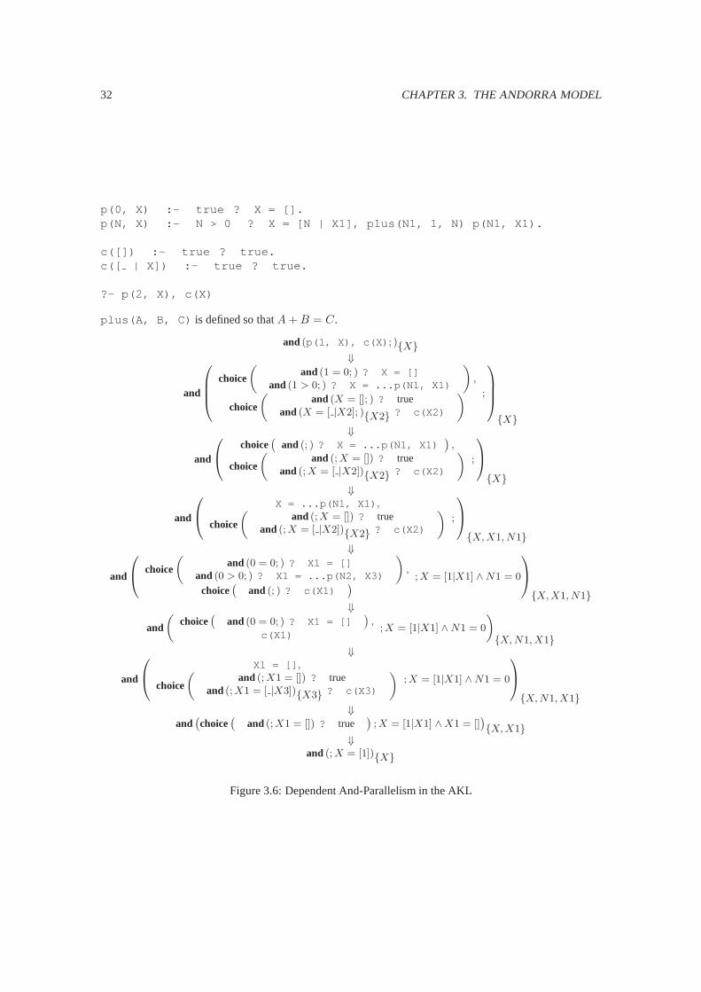
32 CHAPTER 3. THE ANDORRA MODEL
p(0, X) :- true ? X = [].p(N, X) :- N > 0 ? X = [N | X1], plus(N1, 1, N) p(N1, X1).
c([]) :- true ? true.c([ | X]) :- true ? true.
?- p(2, X), c(X)
plus(A, B, C) is defined so thatA+B = C.
and(p(1, X), c(X) ; ){X}⇓
and
choice
(and(1 = 0; ) ? X = []
and(1 > 0; ) ? X = ...p(N1, X1)
),
choice
(and(X = []; ) ? true
and(X = [ |X2]; ){X2} ? c(X2)
) ;
{X}
⇓
and
choice
(and (; ) ? X = ...p(N1, X1)
),
choice
(and(; X = []) ? true
and(; X = [ |X2]){X2} ? c(X2)
);
{X}
⇓
and
X = ...p(N1, X1) ,
choice
(and(; X = []) ? true
and(; X = [ |X2]){X2} ? c(X2)
);
{X, X1, N1}
⇓
and
choice
(and(0 = 0; ) ? X1 = []
and(0 > 0; ) ? X1 = ...p(N2, X3)
),
choice(
and (; ) ? c(X1)) ; X = [1|X1] ∧ N1 = 0
{X, X1, N1}
⇓and
(choice
(and(0 = 0; ) ? X1 = []
),
c(X1); X = [1|X1] ∧ N1 = 0
){X, N1, X1}
⇓
and
X1 = [] ,
choice
(and(; X1 = []) ? true
and(; X1 = [ |X3]){X3} ? c(X3)
); X = [1|X1] ∧ N1 = 0
{X, N1, X1}
⇓and
(choice
(and(; X1 = []) ? true
); X = [1|X1] ∧ X1 = []
){X, X1}
⇓and (; X = [1]){X}
Figure 3.6: Dependent And-Parallelism in the AKL

3.4. ANDORRA KERNEL LANGUAGE 33
p(X, Y) :- X = a ? Y = c.p(X, Y) :- X = b ? Y = b.p(X, Y) :- X = c ? Y = a.
?-p(X)
and(p(X, Y) ; true){X, Y }⇓
and
(choice
(and (X = a; true) ? Y = cand (X = b; true) ? Y = band (X = c; true) ? Y = a
); true
){X, Y }
⇓
and
(choice
(and(; X = a) ? Y = cand(; X = b) ? Y = band(; X = c) ? Y = a
); true
){X, Y }
⇓
or
and (Y 1 = c; X1 = a){X1, Y 1}and
(choice
(and(; X = b) ? Y = band(; X = c) ? Y = a
); true
){X, Y }
⇓
or
and(; X1 = a ∧ Y 1 = c){X1, Y 1}and(Y 2 = b; X2 = b){X2, Y 2}and
(choice
(and(; X = c) ? Y = a
); true
){X, Y }
⇓
or
and(; X1 = a ∧ Y 1 = c){X1, Y 1}and(; X2 = b ∧ Y 2 = b){X2, Y 2}and(Y = a; X = c){X, Y }
⇓
or
and(; X1 = a ∧ Y 1 = c){X1, Y 1}and(; X2 = b ∧ Y 2 = b){X2, Y 2}and(; X = c ∧ Y = a){X, Y }
Figure 3.7: Or-Parallelism in the AKL

34 CHAPTER 3. THE ANDORRA MODEL

Chapter 4
The AKL and Logic
Since the AKL is intended to be alogic programming language, an AKL program is intended to have alogical semantics. This chapter covers the logical structure of the AKL, and introduces a fixpoint semanticsfor the language that can be used as the concrete semantics for abstract interpretation (see chapter6). Thischapter builds upon the work of Fitting [Fit91] on applying bilattices to logic programming and applies thebilattice model to committed-choice languages in general and the AKL in particular.
4.1 Logical Aspects of the AKL
Before considering the logical aspects of the AKL, it is necessary to provide an intended interpretation of anAKL program. The intended interpretation maps a programP onto a set of logical formulaeΣP . The AKLexecution model should be sound in the sense that any answer computed should be a logical consequenceof ΣP , and complete in the sense that all possible logical consequences ofΣP are computed.
The basic logical structure of AKL program is given in [Fra94]. A constraint theory,T C, is assumed,with a constraint,σ, holding ifT C |= σ. Each predicate in the program is given a completed definition:
Definition 4.1.1 Thecompleted definition, ΣP of an AKL programP is given by replacing each predicatep/n :
p(x) :- G1(x,y) % B1(x,y)· · ·
p(x) :- Gm(x,y) % Bm(x,y)
by:
∀xp(x)↔
∃y1(G1(x,y1) ∧B1(x,y1))∨
· · · ∨∃ym(Gm(x,ym) ∧Bm(x,ym))
if % is ? or | . If % is -> , the predicate is replaced by:
∀xp(x)↔
∃y1(G1(x,y1) ∧B1(x,y1))∨(¬∃y1(G1(x,y1)) ∧ ∃y2(G2(x,y2) ∧B2(x,y2))∨
· · · ∨
¬∃y1(G1(x,y1))∧· · · ∧
(¬∃ym−1(G1(x,ym−1))∧∃ym(Gm(x,ym) ∧Bm(x,ym)
The boldfacex, y andz are used to represent vectors of variables.
35

36 CHAPTER 4. THE AKL AND LOGIC
4.1.1 Negation
Negation as failure is introduced into the AKL by using conditional guards. Ifp(X) is a predicate, thennot p(X) is given by
not p(X) :- p(X) -> false.not p(X) :- true -> true.
or more usefully, since we are only interested in seeing whether one branch succeeds,
not p(X) :- some p(X) -> false.not p(X) :- true -> true.
some p(X) :- p(X) | true.
4.1.2 Commit Guards
The presence of the commit operator (| ) in the AKL tends to produce difficulties with negation. Considerthe standard definition formerge/3 :
merge([], B, O) :- | O = B.merge(A, [], O) :- | O = A.merge([X | A], B, O) :- | O = [X | O1], merge(A, B, O1).merge(A, [X | B], O) :- | O = [X | O1], merge(A, B, O1).
A query such asmerge([1], [2], [1, 2]) may succeed or fail, depending on the exact path ofthe computation. Similarly,merge([1], [2], X), not merge([1], [2], X) may succeed,breaking the identityA ∧ ¬A ≡ false.
Franzen [Fra94] avoids the difficulties with commit by examining only those predicates with authorita-tive guards:
Definition 4.1.2 An AKL program,P , is authoritativeif for every clause of the form
H(x) :- G(x,y) | B(x,y, z).
in P
T C ∪ ΣP |= G(x,y)→ (H(x)↔ ∃zB(x,y, z))
Authoritative guards guarantee that it does not matter which clause is chosen, in the case of two guardssucceeding, as both bodies produce the same results. An example of a predicate with authoritative guardsis:
min(X, Y, Z) :- X =< Y | Z = X.min(X, Y, Z) := X >= Y | Z = Y
Authoritative guards restrict the commit operator to simply pruning equivalent solutions to the predicate.Unfortunately,merge/3 is not authoritative, excluding a large class of reactive programs from this logicalinterpretation of the AKL.

4.2. A BILATTICE INTERPRETATION OF AKL PROGRAMS 37
4.1.3 Conditional Guards
Nondeterminate promotion within a conditional guard can produces cases where the guard prunes alterna-tives within the guard computation that are implied by the completed definition (definition4.1.1). As anexample, consider the program:
p :- r(X) -> X = a.
r(X) :- ? X = b.r(X) :- ? X = a.
In this case,p/0 will fail, as the second solution tor(X) is pruned. However, the completed definitionof r/1 is ∀Xr(X) ↔ (X = b ∨X = a) and therefore that ofp/0 is p ↔ true. The solution adopted byFranzen is to restrict the set of programs examined to those with indifferent guards:
Definition 4.1.3 An AKL program,P , is indifferentif, for every clause of the form
H(x) :- G(x,y) -> B(x,y, z).
in P ,T C ∪ ΣP |= G(x,y) ∧G(x,w)→ (∃zB(x,y, z)↔ B(x,w, z))
Most AKL programs are intended to be indifferent, although an insistence on indifference eliminatesonce/1 -style predicates written with conditional guards, which are intended to accept the first solution toa query. Such predicates can be used to accept a single permutation of some set of values, such as a registerallocation. However these predicates can be re-cast as commit-guarded predicates without damaging theintended behaviour of the predicate.
4.1.4 Recursive Guards
Recursive guards present a problem in the AKL, as it is possible for a program to enter an infinite loop, eventhough the logical semantics for the program have a definite value. As an example, consider the predicatep/1 :
p(0).p(s(X)) :- p(X) ? true.
Calling this program with?-p(s(s(s(0)))) will result in a response oftrue . However callingthis program with the query?-p(X) will result in an infinite loop, as the recursive guard is tried within anew environment with each local fork. Since the AKL always expands guards (a deterministic operation)in preference to nondeterminate promotion, this query will never terminate.
Generally, recursive guards should be avoided in the AKL; they produce infinite loops and make theprogram unstratified, since a recursive call within a conditional guard results in a recursive form of negation.For this reason only guard-stratified programs are used.
Definition 4.1.4 A programP is guard-stratifiedif it can be partitioned into programsP1, . . . , Pl withP1 ∪ · · · ∪ Pl = P such that each guard of each clause inPk contains only primitive constraints, or atomsdefined by clauses inP1 ∪ · · · ∪ Pk−1
4.2 A Bilattice Interpretation of AKL Programs
The introduction of authoritative AKL programs weakens the number of uses that a logical interpretation ofAKL can be put to. Authoritative guards are intended to eliminate the situations where a query can eithersucceed or fail, keeping the logical definition within the bounds of a classical two-valued logic, with successmapping onto true and failure onto false.
An alternative to insisting on authoritative guards is to move beyond two-valued logic, and introduce amulti-valued logic which contains a value that maps on to the notion of “sometimes succeeds — sometimesfails.”

38 CHAPTER 4. THE AKL AND LOGIC
HHHHHHHH
HHHHHHHH
��������
6
-
��������
>
v
⊥
false true
≤
Figure 4.1: The logicFOUR
4.2.1 Bilattices
Bilattices were introduced to logic programming by Fitting [Fit91] with the intention of modelling uncertainand unknown information. The characterisation of bilattices given here is taken from [Fit91], with somechanges in notation1.
Definition 4.2.1 An interlaced bilatticeis a set,B, together with two partial orderings,≤ andv, such that:
1. each of≤ andv givesB the structure of a complete lattice.
2. the lub and glb operations for each partial ordering are monotone with respect to the other partialordering.
4.2.2 A Logic Based on FOUR
The AKL, needs the simplest form of bilattice,FOUR[Bel77]. The Hasse diagram forFOUR is shown infigure4.1.
For the purposes of the AKL,> is interpreted as meaning “both succeeds and fails” and⊥ has a meaningof undefined, which can be interpreted as either “still being computed,” “infinite loop” or “deadlocked,”depending on context. The values true and false are interpreted as “always succeeds” and “always fails.”With these meanings,v can be interpreted as an ordering on the range of possible results a program cangive.
The standard Boolean operations of logical and (∧), or (∨) and not (¬) now have a set of dual operationsbased on thev ordering: indecisive-and (u), indecisive-or (t) and indecisive-not (−) 2. Using theFOURbilattice, the standard Boolean operators, and their duals, are given in table4.1. The four basic operators arederived froma ∧ b ≡ glb≤(a, b), a ∨ b ≡ lub≤(a, b), a u b ≡ glbv(a, b) anda t b ≡ lubv(a, b). Negationis a reflection about thev axis and indecisive negation a reflection about the≤ axis. Implication is definedby a→ b ≡ ¬− a ∨ b and equivalence bya↔ b ≡ (a→ b) ∧ (a← b).
The quantification operators can be interpreted as conjunction or disjunction over the domain of a vari-able:∃xa(x) ≡
∨y∈dom(x) a(y) and∀xa(x) ≡
∧y∈domx a(y)
3.
1In this thesis,≤ is used instead of the≤t in [Fit91]. Similarly, v is used in place of≤k, u in place of⊗ andt in place of⊕.2 These names derive from the idea that indecisive-or can’t make up its mind about truetfalse; the initial motivation for introducing

4.2. A BILATTICE INTERPRETATION OF AKL PROGRAMS 39
a b a ∧ b a ∨ b a u b a t b ¬a −a a→ b a↔ btrue true true true true true false true true truetrue > > true true > false true > >true ⊥ ⊥ true ⊥ true false true ⊥ ⊥true false false true ⊥ > false true false false> true > true true > > ⊥ true >> > > > > > > ⊥ true true> ⊥ false true ⊥ > > ⊥ ⊥ false> false false > false > > ⊥ ⊥ ⊥⊥ true ⊥ true ⊥ true ⊥ > > ⊥⊥ > false true ⊥ > ⊥ > true false⊥ ⊥ ⊥ ⊥ ⊥ ⊥ ⊥ > > true⊥ false false ⊥ ⊥ false ⊥ > true >false true false true ⊥ > true false true falsefalse > false > false > true false true ⊥false ⊥ false ⊥ ⊥ false true false true >false false false false false false true false true true
Table 4.1: Boolean operators forFOUR
The combination ofFOUR and the operations defined above form an extended Boolean algebra, sat-isfying the normal identities of a Boolean algebra. These identities are summarised in table4.2; most areconsequences of the properties of interlaced bilattices (see [Fit91]).
4.2.3 Commit Predicates
Armed with the bilattice described above, it is now possible to describe a logical interpretation of a commit-guarded predicate. If two guards can potentially succeed and one body succeeds and the other body fails,then the truth-values of these two clauses can be combined via indecisive-or into a truth-value of>.
Intuitively the failure of a guard should give the clause a truth-value of⊥. This means that the clausewill not appear in the truth-value of the predicate. A guard operator should have the following properties:
a‖b ={⊥ if a = ⊥ or a = falseb otherwise
This guard operator can be defined asa‖b ≡ (¬a t true) u (a t false) u b.All predicates in the AKL follow the negation as failure rule; if no clause succeeds, then a truth value
of false is assumed. As a special case, all guard operators failing is also assumed to mean a truth value offalse. With the above definition ofa‖b, all guards failing will yield a truth value of⊥. While this truthvalue may be aesthetically satisfying it does not match the definition of the language, and an explicit termfor failure needs to be introduced. If a predicate is defined by a set of clauses,
H(x) :- Gi(x,y) | Bi(x,y, z), 1 ≤ i ≤ n,
then the additional term for failure can be defined as:
fail(G1, . . . , Gn) ={
false if allGi are false or>⊥ otherwise
fail(G1, . . . , Gn) ≡ G1 u · · · uGm u false matches this definition.
a multi-valued logic. In [Fit91] indecisive-not is called confluence.3 Similar quantification operators can be defined for the indecisive operators. These operators play no part in the fixpoint semantics
for the AKL and are therefore ignored.

40 CHAPTER 4. THE AKL AND LOGIC
Nulla ∧ false= false a ∨ true= truea u ⊥ = ⊥ a t > = >Identitya ∧ true= a a ∨ false= aa u > = a a t ⊥ = aIdempotenta ∧ a = a a ∨ a = aa u a = a a t a = aInverse¬¬a = a −− a = aa ∧ ¬ − a = false a ∨ ¬ − a = truea u ¬ − a = ⊥ a t ¬ − a = >Commutativea ∧ b = b ∧ a a ∨ b = b ∨ aa u b = b u a a t b = b t aAssociative(a ∧ b) ∧ c = a ∧ (b ∧ c) (a ∨ b) ∨ c = a ∨ (b ∨ c)(a u b) u c = a u (b u c) (a t b) t c = a t (b t c)Distributivea ∧ (b ∨ c) = (a ∧ b) ∨ (a ∧ c) a ∧ (b u c) = (a ∧ b) u (a ∧ c)a ∧ (b t c) = (a ∧ b) t (a ∧ c)a ∨ (b ∧ c) = (a ∨ b) ∧ (a ∨ c) a ∨ (b u c) = (a ∨ b) u (a ∨ c)a ∨ (b t c) = (a ∨ b) t (a ∨ c)a u (b ∧ c) = (a u b) ∧ (a u c) a u (b ∨ c) = (a u b) ∨ (a u c)a u (b t c) = (a u b) t (a u c)a t (b ∧ c) = (a t b) ∧ (a t c) a t (b ∨ c) = (a t b) ∨ (a t c)a t (b u c) = (a t b) u (a t c)Absorptiona ∧ (a ∨ b) = a a ∨ (a ∧ b) = aa u (a t b) = a a t (a u b) = aDeMorgan’s¬(a ∧ b) = ¬a ∨ ¬b ¬(a ∨ b) = ¬a ∧ ¬b¬(a u b) = ¬a u ¬b ¬(a t b) = ¬a t ¬b−(a ∧ b) = −a ∧−b −(a ∨ b) = −a ∨−b−(a u b) = −a t−b −(a t b) = −a u−b
Table 4.2: Boolean identities onFOUR

4.3. A FIXPOINT SEMANTICS FOR THE AKL 41
FOUR can now be used to give a logical interpretation of the AKL. The interpretations of? and-> guarded predicates are the same as section4.1. A set of commit-guarded clauses,
H(x) :- Gi(x,y) | Bi(x,y, z), 1 ≤ i ≤ n,
now has the logical interpretation:
∀xH(x)↔
∃y1(G1(x,y1)‖B1(x,y1))t· · · t
∃ym(Gm(x,ym)‖Bm(x,ym))t(∃y1G1(x,y1) u · · · u ∃ymGm(x,y) u false)
4.3 A Fixpoint Semantics for the AKL
A fixpoint semantics for the AKL can now be derived in terms of some suitable immediate consequencesoperator. The treatment here follows that of [Fit91].
Definition 4.3.1 An interpretationis a mappingv from a subset of ground atomic formulae toFOUR. Theinterpretation isin the constraint theoryT C provided that for each constraintθ, if T C |= θ thenvθ = trueand ifT C 6|= θ thenvθ = false.I denotes the domain of interpretations.
It may be possible to extend the constraint theory to handle the full four values ofFOUR. However, theproofs of the soundness and completeness theorems (theorems4.4.1and4.4.2) require constraints to onlyhave two values.
Throughout this section functional notation is used to reduce the number of parentheses;v θ is inter-preted as the application of the mappingv to the argumentθ.
Definition 4.3.2 Thecompositionof two interpretations,v1 andv2, denoted byv1 � v2, is defined as
(v1 � v2)A ={v1A if A ∈ dom(v1)v2A otherwise
Definition 4.3.3 Given two interpretationsv1 and v2, v1 ≤ v2 if for all closed atomic formulaeA ∈dom(v1), v1A ≤ v2A. A similar definition holds forv.
Definition 4.3.4 If v is an interpretation andφ a closed formula, thenvφ is constructed by interpreting∧in φ as∧ onFOUR, ∨ in φ as∨ onFOUR, etc.
An immediate consequences operator for an AKL program can now be defined. The immediate conse-quences operator is intended for use on guard stratified program. The operator takes two arguments: the firstargument is the interpretation provided by previous stratifications, the second is the current interpretation.
Definition 4.3.5 LetP be an AKL program.ΦP : I → I → I is defined as follows:
1. If H(x) :- Gi(x,y) ? Bi(x,y, z) ∈ P then
ΦP p v H(x) = (p � v)
∃y1, z1G1(x,y1) ∧B1(x,y1, z1)∨
· · · ∨∃ym, zmGm(x,ym) ∧Bm(x,ym, zm)

42 CHAPTER 4. THE AKL AND LOGIC
2. If H(x) :- Gi(x,y) -> Bi(x,y, z) ∈ P then
ΦP p vH(x) = (p � v)
∃y1, z1G1(x,y1) ∧B1(x,y1, z1)∨· · · ∨
¬∃y1G1(x,y1)∧. . .∧¬∃ym−1Gm−1(x,ym−1)∧∃ym, zmGm(x,ym) ∧Bm(x,ym, zm)
3. If Hi((x)) :- Gi(x,y) | Bi(x,y, z) ∈ P then
ΦP p v H(x) = (p � v)
∃y1, z1G1(x,y1))‖B1(x,y1, z1)t· · · t
∃ym, zmGm(x,ym))‖Bm(x,ym, zm)t(∃y1G1(x,y1) u · · · u ∃ymGm(x,ym) u false)
4. ΦP p v φ = (p � v)φ otherwise.
Definition 4.3.6 GivenP , an indifferent, guard stratified program , withQ as one of the stratifications, andan interpretation,p, then:
ΦQ p ↑ 0 = p.ΦQ p ↑ α = ΦQ p(ΦQ p ↑ (α− 1)), if α is a successor ordinal.ΦQ p ↑ α = lub{ΦQ p ↑ β : β < α}, if α is a limit ordinal.
Proposition 4.3.1 SupposeP is an indifferent, guard stratified program, partitioned into sub-programs{P1, . . . , Pm}. Further suppose that there exists an interpretation,p, which is inT C, and has a domaincovering all guards inPi = Q. ThenΦQ p is continuous.
Proof The proof is a suitable variation of that in [Llo84]. ΦQ p is continuous iflub(ΦQ pX) =ΦQ p lub(X) for all directed sets X.
Since both≤ andv are defined in a pointwise fashion on interpretations (definition4.3.3), it is clearthat lub(X)φ = lub(X φ) for all formulaeφ ∈
⋃dom(X) for both orderings.
ΦQ p lub(X)H = t, t ∈ FOURiff H ↔ φ ∈ ΣQ and lub(X)φ = tiff H ↔ φ ∈ ΣQ and lub(X φ) = tiff lub(ΦQ pX H) = t 2
Corollary 4.3.1 ΦQ p has a least fixpoint and greatest fixpoint, with lfp(ΦQ p) = ΦQ p ↑ ω. See [Llo84].
Theorem 4.3.1 (Fixpoint characterisation of the AKL)Suppose P is an indifferent, guard stratified program, partitioned into sub-programs
{P1, . . . , Pm}. Further suppose thatp is a model inT C for P1 ∪ · · · ∪Pi−1. ThenΦPi p ↑ ω is a model forT C ∪ P1 ∪ · · · ∪ Pi.
Proof This proof is, again, a variation on [Llo84]. To start with,v is a model forPi if ΦPi p v v v sincev is a model forPi if, for eachH ↔ φ ∈ ΣPi , v H = v φ. SinceΦPi p ↑ ω = lfp(ΦPi p) it follows thatΦPi p (ΦPi p ↑ ω) v ΦPi p ↑ ω. 2

4.4. THE AKL EXECUTION MODEL 43
4.4 The AKL Execution Model
The fixpoint semantics for the AKL derived in section4.3provide a suitable model for the intended mean-ing of an AKL program. However, the AKL itself follows a top-down execution model and it becomesnecessary to derive the relationship between the fixpoint semantics and the execution model.
The AKL execution model consists of a series of transitions over configurations. IfA andB are con-figurations (as defined in section3.4) thenA ⇒t B is a derivation fromA to B via the execution rulet. If the execution rule is obvious from the context, thenA ⇒ B is a suitable shorthand. Multiple un-specified transitions, can be written asA ⇒∗ B. A configurationA is a terminal configurationif thereexists no admissible transitionA ⇒ B. A terminal configurationA is anend configurationif A has theform choice
(and(; θ1)vars(θ1)
? true , . . . ,and(; θn)vars(θn) ? true). Terminal configurations
that are not end configurations aredeadlock configurations.A logical mapping for AKL configurations is also necessary. Following the model of sections4.1and
4.2.3each box can be mapped onto a logical interpretation in a manner similar to that of [Fra94], butadjusted to the new definition for commit.
Definition 4.4.1 Thelogical interpretationof a configurationC, written asC∗, is defined recursively as:
1. fail∗ = false.
2. A∗ = A, whereA is an atom or primitive constraint. In particular,true ∗ = true.
3. (A,B)∗ = A∗ ∧B∗
4. and(R; θ)∗V = ∃V (R∗ ∧ θ).
5. choice(G1 ? B1, . . . , Gn ? Bn
)∗ = G∗1 ∧B∗
1 ∨ · · · ∨G∗n ∧B∗
n.
6. choice(G1 -> B1, . . . , Gn -> Bn
)∗ = G∗1 ∧B∗
1 ∨ · · · ∨ ¬G∗1 ∧ · · · ∧ ¬G∗
n−1 ∧G∗n ∧B∗
n.
7. choice(G1 | B1, . . . , Gn | Bn
)∗ = G∗1‖B∗
1 t · · · tG∗n‖B∗
n t (G∗1 u · · · uG∗
n u false).
8. or(C1, . . . , Cn
)∗ = C∗1 ∨ · · · ∨ C∗
n
Lemma 4.4.1 Given a programP with modelv and an initial goalG, and the transition sequenceA =choice
(and(G; true)vars(G) ? true
)⇒∗ B thenvB∗ v v∃G.
Proof The proof proceeds by induction on the number of transitions. Clearly, for zero transitions,vA∗ =v∃G. Suppose that the proposition holds forA ⇒∗ C and the next transition in the sequence isC ⇒t B,then each transition can be examined:
In the cases of constraint imposition, environment synchronisation, failure propagation, determinatepromotion and non-determinate promotion, the transition is a re-arrangement of the expressionC∗ follow-ing the identity rules ofFOUR. ObviouslyvB∗ = vB∗.
In the case of local forking, the transition isH ⇒ choice
(and(G1; true)vars(G1) % B1, . . . ,and(Gn; true)vars(Gn) % Bn
)for someH . Since
H ↔ φ ∈ ΣP hasφ given by definitions in4.1.1and section4.2.3, and these are the same as the definitiongiven in definition4.4.1, it must be thatvC∗ = vB∗.
In the case of an application of the cut rule, there exists a final guardG = and(; θ)V andvG = truesinceT C |= θ. In this case all subsequent guards have¬G in them, and must therefore havev¬G = false.From the identity rules ofFOUR, vC∗ = vB∗.
If a commit rule is applied, then all surroundingt parts of the expression inC∗ are removed. Sincetis defined in terms of lub onv it follows thatC∗ v B∗. 2
Lemma4.4.1can be used to provide a soundness theorem for the AKL:

44 CHAPTER 4. THE AKL AND LOGIC
Theorem 4.4.1 (Soundness of AKL) IfP is an indifferent, stratified AKL program,G a goal andchoice
(and(G; true)vars(G) ? true
)⇒∗ B whereB is an end configuration, thenΣP ∪ T C |=
B∗ v ∃G
Proof By application of lemma4.4.12
In theorem4.4.1, B will be a collection of constraints which are modelled byT C. Thev is necessary,rather than implication, sinceG may have a truth value of> and true→ > has a truth value of>.
Theorem4.4.1also serves as a proof of soundness of failure, since the end configuration may befail .Completeness is a little more difficult for AKL programs. Assuming that the program actually termi-
nates, then it is not possible for completeness to be meaningfully defined for programs that have predicateswith a truth value of>. However completeness is possible for the subset of authoritative AKL programsand queries that terminate.
Theorem 4.4.2 (Completeness of AKL) IfP is an authoritative, indifferent, guard stratified AKL program,G a goal andchoice
(and(G; true)vars(G) ? true
)⇒∗ B whereB is an end configuration then
ΣP ∪ T C |= ∃G↔ B∗
Proof If P is authoritative, then using definition4.1.2, it is not possible forG to have a truth value of>.B consists only of constraints, and constraints must have a truth value of true or false. SinceΣP ∪ T C |=B∗ v ∃G, B∗ is true or false and∃G is either true, false or⊥ then∃G is either true or false and therefore,from the Hasse diagram ofFOUR ΣP ∪ T C |= G↔ B∗. 2
The above theorem also shows the relationship between the logical semantics derived by the fixpointconstruction given here and the semantics given in [Fra94]. Provided a program is authoritative, indifferentand guard stratified, no goal has a truth-value of> and (with the exception of undefined goals — thosehaving a truth value of⊥) the true and false truth values must match.
Since there is a value of⊥ for undefined truth values, a more accurate model of the truth value of anAKL configuration can be derived by giving unevaluated atoms a truth value of⊥.
Definition 4.4.2 The execution interpretationof a configurationC, written asC+ is the same as that ofthe logical interpretation ofC, replacing all instances of∗ by + with the exception of case 2. For case 2A+ = ⊥ if A is an atom or primitive constraint.
Lemma 4.4.2 Given a programP with modelv and a configurationC, thenv(C+) v v(C∗).
Proof Both C∗ andC+ are monotone with respect to their sub-components. This is clearly true in allcases except case 7 in definition4.4.1, since the∧ and∨ operations are monotone onv. In case 7, thetoperator builds alub of its arguments and is therefore also monotone onv.
Since the difference betweenC∗ andC+ is thatC+ replaces any atomA with ⊥ instead ofv(A) and⊥ v v(A) it follows thatC+ v C∗. 2
4.5 Some Examples
This section gives some examples of theΦP operator acting on programs with various degrees of well-behavedness. For convenience,ΦPi is used instead ofΦPi (ΦPi−1 ↑ ω).

4.5. SOME EXAMPLES 45
p(X, Y) :- X = a ? Y = b. q(X, Y) :- p(X, Y) -> true.p(X, Y) :- X = b ? Y = a. q(X, Y) :- p(X, Z) -> q(Z, Y).
P1 = {p/2 }
ΦP1 ↑ 0 = {p(X, Y ) ↔ ⊥}ΦP1 ↑ 1 = {p(X, Y ) ↔ (X = a ∧ Y = b) ∨ (X = b ∧ Y = a)}
ΦP1 ↑ ω = ΦP1 ↑ 1
P2 = {q/2 }
ΦP2 ↑ 0 = ΦP1 ↑ ω ∪ {q(X, Y ) ↔ ⊥}
ΦP2 ↑ 1 = ΦP1 ↑ ω ∪
q(X, Y ) ↔
(X = a ∧ Y = b) ∨ (X = b ∧ Y = a)∨(
(¬(X = a ∧ Y = b) ∨ (X = b ∧ Y = a))∧∧(X = a ∨ X = b) ∧ ⊥
)
ΦP2 ↑ 2 = ΦP1 ↑ ω ∪
q(X, Y ) ↔
(X = a ∧ Y = b)∨(X = b ∧ Y = a)∨(X = a ∧ Y = a)∨(X = b ∧ Y = b)
ΦP2 ↑ ω = ΦP2 ↑ 2
Figure 4.2: A Guard Stratified, Indifferent, Authoritative Program
p(X, Y) :- X = a | Y = b.p(X, Y) :- X = a | Y = a.
q :- p(a, b).
P1 = {p/2 , q/0 }
ΦP1 ↑ 0 = {p(X, Y ) ↔ ⊥, q ↔ ⊥}
ΦP1 ↑ 1 =
{p(X, Y ) ↔
(((X 6= a t true) u (X = a t false) u Y = bt((X 6= a t true) u (X = a t false) u Y = at
(X = a u false)
), q ↔ ⊥
}
ΦP1 ↑ 2 =
{p(X, Y ) ↔
(((X 6= a t true) u (X = a t false) u Y = bt((X 6= a t true) u (X = a t false) u Y = at
(X = a u false)
), q ↔ >
}
ΦP1 ↑ ω = ΦP1 ↑ 2
Figure 4.3: A Guard Stratified, Indifferent Program

46 CHAPTER 4. THE AKL AND LOGIC
p :- p
q(X) :- p | X = a.q(X) :- true | X = b.
P1 = {p/0 }
ΦP1 ↑ 0 = {p ↔ ⊥}ΦP1 ↑ ω = ΦP1 ↑ 0
P2 = {q/1 }
ΦP2 ↑ 1 = ΦP1 ↑ ω ∪ {q(X) ↔ ⊥}ΦP2 ↑ 1 = ΦP1 ↑ ω ∪ {q(X) ↔ X = b}
ΦP2 ↑ ω = ΦP2 ↑ 1
Figure 4.4: A Guard Stratified, Indifferent Program with Looping
4.5.1 Well-Behaved Programs
Well-behaved programs are guard stratified and indifferent. An example well-behaved program, which isalso authoritative, is shown in figure4.2. In this programq/2 computes the transitive closure ofp/2 , witha conditional guard to ensure thatq/2 is used for queries only.
An example non-authoritative, well-behaved program is shown in figure4.3. In this case a race conditionexists between the two clauses ofp/2 , which will result in a query toq/0 either succeeding or failing. Asa resultq/0 has a truth value of>.
Another example of a well-behaved program is a program with an infinite loop in it. In figure4.4, p/0has no single truth value and so retains a truth value of⊥. If this truth value is fed into the guard ofq/1then the other clause completely describes the predicate. Operationally, if the computation rule is fair, thesecond guard ofq/2 will succeed before the first guard and prune the first guard away.
The fixpoint for the semantics does not necessarily perfectly reflect the actual behaviour of an AKLprogram. Clearly if the commit rule prunes unfairly then some of the success configurations implied by thefixpoint semantics will never be reached. The fixpoint semantics take no account of modes, which can leadto certain unreachable configurations being defined as true. For example, the program
p(X, Y) :- X = a | Y = b.p(X, Y) :- X = b | Y = a.
q(X, Y) :- true | Y = a.q(X, Y) :- X = a | Y = b.
r(X) :- p(X, Y), q(Y, X).
has a fixpoint of
p(X,Y )↔ (X = a‖Y = b) t (X = a‖Y = b) t (X = a uX = b u false)q(X,Y )↔ Y = a t (X = a‖Y = b)r(X)↔ (X = a tX = b)
This fixpoint for r/1 is correct if r/1 is called with a fully constrained argument —?-r(b) mayfail, depending on whetherp(b, Y) or q(Y, b) is first called. However ifr/1 is called with an uncon-strained argument, then only one solution can be reached:X = a.

4.5. SOME EXAMPLES 47
p(X) :- true ? X = a.p(X) :- true ? X = b.
one p(X) :- p(Y) -> X = Y.P1 = {p/1 }
ΦP1 ↑ 0 = {p(X) ↔ ⊥}ΦP1 ↑ 1 = {p(X) ↔ (X = a ∨ X = b)}
ΦP1 ↑ ω = ΦP1 ↑ 1
P2 = {one p/1 }
ΦP2 ↑ 0 = ΦP1 ↑ ω ∪ {one p(X) ↔ ⊥}ΦP2 ↑ 1 = ΦP1 ↑ ω ∪ {one p(X) ↔ (X = a ∨ X = b)}
ΦP2 ↑ ω = ΦP2 ↑ 1and (one p(X) ; ){X}
⇓∗
and
(choice
(and(
choice(
and (; ) ? Y = aand (; ) ? Y = b
);){Y }
-> X = Y
);
){X}
⇓∗
and
(choice
(and (; Y = a){Y } -> X = Y
and (; Y = b){Y } -> X = Y
);
){X}
⇓∗
and(
choice(
and (; Y = a){Y } -> X = Y)
;){X}
⇓∗and (; X = a){X}
Figure 4.5: A Non-Indifferent Program
4.5.2 Non-Indifferent Programs
Figure4.5shows a program which is not indifferent, along with its fixpoint and the actual AKL computationwhich will occur.
The AKL computation implies a fixpoint of
ΦP2 ↑ ω = {p(X)↔ (X = a ∨X = b), one p(X)↔ X = a}
which contains less possible successes than the fixpoint computed by theΦP operator. Since non-indifferentprograms contain alternate solutions within their guards, some of which will be pruned away by the condi-tional guard operator, non-indifferent programs generally succeed less times than the fixpoint would imply.Non-indifference in conditional guards contains some similarities to red cuts, so this behaviour is not unex-pected.
4.5.3 Non-Guard Stratified Programs
Figure4.6shows a non-guard stratified program, along with its fixpoint derived fromΦP and an examplecomputation. Not being guard stratified does not prevent a program from having its fixpoint calculated.However non guard-stratified programs contain hidden infinite loops which are caused by new environmentscontained in the guards being able to speculatively bind unconstrained arguments and continue. If the query?-e(s(s(0))) was tried, the program would terminate.
Guard stratification is not strictly needed to make negation monotone, as is the case with stratificationof negation using theTP operator. Predicates within guards are not assumed to be false, but rather⊥ untilthey are completely computed. As an example,
p :- not q.
q :- not p.
simply has a fixpoint of{p↔ ⊥, q ↔ ⊥}.

48 CHAPTER 4. THE AKL AND LOGIC
e(0).e(s(X)) :- o(X) ? true.o(s(X)) :- e(X) ? true.
P1 = {e/1 , o/1 }
ΦP1 ↑ 0 = {e(X) ↔ ⊥, o(X) ↔ ⊥}ΦP1 ↑ 1 =
{e(X) ↔ (X = 0 ∨ (X = s(X1) ∧ ⊥)),
o(X) ↔ (X = s(X1) ∧ ⊥)
}
ΦP1 ↑ 2 =
{e(X) ↔ (X = 0 ∨ (X = s(s(X1)) ∧ ⊥)),o(X) ↔ (X = s(0) ∨ (X = s(s(X1)) ∧ ⊥)
}
ΦP1 ↑ 3 =
{e(X) ↔ (X = 0 ∨ X = s(s(0) ∨ (X = s(s(s(X1))) ∧ ⊥)),
o(X) ↔ (X = s(0) ∨ (X = s(s(s(0))) ∨ (X = s(s(X1)) ∧ ⊥)
}...
and (e(X) ; ){X}⇓∗
and
(choice
(and (; X = 0) ? true ,
and (o(X1) ; X = s(X1)){X1} ? true ,
);
){X}
⇓∗
and
(choice
(and (; X = 0) ? true ,
and
(choice
(and (; X1 = s(0)) ? true ,
and (o(X2) ; X1 = s(s(X2))){X2} ? true ,
); X = s(X1)
){X1}
? true ,
);
){X}
.
.
.
Figure 4.6: A Non-Guard Stratified Program
4.6 Related Work
TheFOUR based logic used above has a strong relationship to the stable model semantics developed byGelfond and Lifschitz [GL88]. The stable model semantics uses two sets: one for successes (S) and one forfailures (F ). An immediate consequences operator is developed that uses bothS andF to construct furtheratoms;H ← S1, . . . , Sn,¬F1, . . . ,¬Fm results inH being included in the nextS if eachSi ∈ S and eachFj ∈ F .
The relationship betweenFOUR and the stable model semantics has been examined by Giordano et al[GMS96]: G ↔ ⊥ if G 6∈ S ∪ F , G ↔ > if G ∈ S ∩ F , G ↔ true if G ∈ S − F andG ↔ false ifG ∈ F − S.
Naish [Nai89] uses four different sets to represent potential success and failure in committed choiceprograms, splitting success sets into definite and potential success sets and failure into definite and potentialfailure sets.
Gabbrielli and Levi [GL92] use an unfolding mechanism to derive a fixpoint semantics for committedchoice programs. The unfolding mechanism is careful to retain the reactive behaviour of the program,ensuring that spurious successes are not possible and that deadlocks are correctly modelled.
The main advantage to usingFOUR for formulating the semantics of a logic program is that the programretains its original logical flavour.

Chapter 5
The DAM
This chapter presents an abstract machine for use with the AKL: Doug’s Abstract Machine, or the DAM.The DAM is intended for parallel execution of AKL programs and, therefore, has a number of featuresintended to model parallel execution. As a preliminary step, two existing abstract machines are described,to provide a foundation for the description of the DAM.
5.1 An Overview of Abstract Machines
Most programming languages have a computation model that can be reduced to a handful of basic opera-tions. For example, Prolog can be reduced, via SLD resolution, to unification, term expansion and branchchoice operations. C can be reduced to arithmetic, control flow and stack operations.
From this perspective, a programming language can be considered to have an ideal machine, whichdirectly models the computation model of the language. The primitive operations for the language can thenbe encoded into a sequence of simple, assembly-like instructions. This “abstract machine” is similar inconception to an ordinary computer architecture, but may allow instructions that are not directly realisableon a real architecture; an example is the normal implementation of unification in Prolog, which may notterminate.
The instruction set, registers, data areas, etc. of an abstract machine can be optimised towards thecomputation model of a particular language. The language can then be compiled into these abstract machineinstructions and executed by an emulator1. The advantages of using an abstract machine and compiler ratherthan an interpreter are obvious: rather than interpreting a program, the emulator does not need to do a greatdeal of work in decoding the program; each instruction tends to be fairly simple and can therefore beoptimised effectively by the emulator; the compiler can be used to statically make optimisation decisionson the abstract instruction set.
This section briefly describes two abstract machines: the WAM and the JAM. Both these machines haveinfluenced the design of the DAM and provide a basis for comparison. The JAM is a parallel implementationof Parlog. The WAM is included as an example of a reasonably efficient abstract machine design for a logicprogramming language (Prolog).
5.1.1 The WAM
The WAM, or Warren Abstract Machine, is an abstract machine formalised for use with Prolog. Elementsfrom the WAM design can be seen in most abstract machines for logic programming languages. A completedescription of the WAM can be found in [War83]. A more approachable description can be found in[AK91a].
The basic WAM architecture consists of three main data areas, a set of registers and an instruction set.These elements are summarised in table5.1. The original WAM specification drew a distinction between
1 Or an actual physical machine, if such a thing is achievable. An example is the CARMEL series of processors for FCP [HG91].
49

50 CHAPTER 5. THE DAM
Heap Stores permanent structuresData Areas Stack Stores temporary structures: environments and choice-
pointsTrail Used to reset some variables that have been bound on
backtrackingPush-Down List A stack for use during unificationP Program pointerCP Continuation pointer (return address)E Environment (stack frame)B Choice-point
Registers A Top of stackH Top of heapTR Top of trailHB Heap position corresponding to creation ofBS Structure pointer into heapX0, X1, ... Temporary registersget constant, ... Get instructionsput constant, ... Put instructionsunify constant, ... Unify instructions
Instructions call, ... Predicate callallocate, ... Environment allocationtry, ... Choice point creationswitch on term, ... Indexing
Table 5.1: Elements of the WAM
the set of temporary registers,X1, X2, ..., and the set of argument registers,A1, A2, .... In actual practise,no distinction needs to be drawn between them. (However, see section5.1.2.)
Execution Model
The WAM treats a Prolog program, suitably encoded into WAM instructions in a similar manner to anordinary imperative-language program. Each predicate call is treated in a similar manner to an imperativelanguage procedure call; arguments are loaded into registers rather than the stack (an advantage whenusing an abstract machine is that you can use a huge number of registers) and the return address is loadedinto theCP register rather than stacked. Argument values and the return address are only stacked whennecessary. Each clause is treated in a similar manner to a procedure definition, with a stack frame (calledthe environment) being used to store local values between calls within the procedure.
The major point of departure from the traditional imperative execution model is the creation of a stackof choice points and a trail. Choice points record snapshots of the WAM state at the start of a predicate call.When the computation fails, usually as the result of a unification failure, the WAM state is unwound backto the first choice point on the stack, a process known as backtracking. This choice point can be used torecover the machine state and then try the next clause in the series of clauses defining a predicate. Uponexecution of the last clause in a predicate, the choice point corresponding to that predicate is removed fromthe stack. A subsequent failure therefore, returns to the previous choice point.
To unwind the state of the WAM, a trail is used to record the changes that have been made since the lastchoice-point was created. When a variable is bound to a new value, the variable is added to the trail stack.Upon failure, the trail is unwound back to the position recorded in the current choice point. Each variablerecorded in the trail is returned to the unbound state.
The WAM provides a primitive form of automatic memory management. New structures are built fromblocks of word-size cells on the heap, the top of which is referenced by theH register. Upon failure, theH register is reset to the position given in the current choice point (and theHB register), recovering anymemory used in speculative computation. The stack register,A, and the trail registerTR are similarly reset.

5.1. AN OVERVIEW OF ABSTRACT MACHINES 51
Successful computations continuously increase the size of the heap and some form of garbage collectionexists in most fully implemented WAM systems.
Representation
The most common representation of structures in the WAM consists of a series of cells. The cells are usuallya convenient word size for the underlying hardware to implement (eg. 32 or 64 bits).
Prolog terms are represented by words containing a value and a tag. The tags take between 2 and 8 bitsand give the type of the term. The remainder of the word usually contains a reference to another term orstructure or, in the case of a constant, the value of the constant. Since all references in the WAM are word-aligned and the value of a term is often a reference to another term, the lower bits of the word are usuallyused to record the tag for references. The tags usually represent variables, constants, integers, references tostructures and references to lists.
Bound and unbound variables share the same tag. Bound variables are represented by containing areference to the term to which the variable is bound or, in the case of a constant, the actual value of theterm representation. Unbound variables are represented by a reference to themselves. Since variables arewords, they can be conveniently manipulated by placing them in registers; taking a copy of the value of anunbound variable turns it into a reference to that variable. A variable is bound to another term by placingthe term representation into the variable’s cell.
Complex structures with an arity greater than 0 are constructed on the heap. The structure consists ofa header cell, containing the structure and its arity, followed byn cells containing the arguments of thestructure. The entire structure is represented by a tagged word containing a reference to the structure. Sincelists are used a great deal in Prolog, lists are simply represented by two cells. A reference to a list is givena different tag to that of a normal structure.
Instructions
Instructions in the WAM are represented by a series of byte codes, followed by arguments and possibleimmediate operands. The instructions can be divided into a number of families.
Get instructions test a register against some term, and if the register is an unbound variable, binds thevariable to that term. If the register fails the test, then the computation fails and backtracking occurs.
Put instructions construct new terms. Put instructions are used to construct the terms used in a predicatecall.
Unify instructions are used to test or construct the arguments of structures. A unify instruction is pre-ceded by a get or put instruction, which puts the WAM into two possible modes: read or write. In readmode, the unify instructions act in a similar manner to get instructions. In write mode the unify instructionsact like put instructions. When a getstructure instruction is executed, the WAM is placed in read mode ifthe argument being examined is bound to a structure, or write mode if the argument is an unbound variable.
Call instructions invoke predicates. Before calling a predicatename/n, the firstn X registers are loadedwith the arguments to the predicate. TheCP register is set to point to the instruction immediately followingthe call instruction andP is set to the address of the code for the predicate being called. At the end of eachclause, a proceed instruction returns by setting theP register back to the value of theCP register.
Environmentsare allocated by use of anallocateinstruction, and deallocated by adeallocateinstruction.Environments save the currentCP register and provide a stack frame with a number of permanent registers,for use if terms need to be stored between predicate calls. The permanent registers take the place of thelocal variables of an imperative language and are referred to asY registers.
Choice pointinstructions control the creation of choice-points. The set of clauses in a predicate isencoded into a try–retry–trust sequence. Try instructions create and initialise a choice point, and try the firstclause in the sequence of possibly matching clauses. Retry instructions follow try instructions and use andupdate the choice point created by the first try instruction. Trust instructions remove the choice point andcommit the computation to the last clause (since all previous clauses have been tried).
Indexinginstructions allow the WAM to restrict the number of clauses tried. An argument to the pred-icate is tested, and if it is bound to a non-variable term, the set of clauses tried can usually be restricted.The switchon term instruction divides the predicate into four classes of clauses, based on the term in the

52 CHAPTER 5. THE DAM
p([]).p([a(X) | Rest]) :- q(f(X), X), p(Rest).
switch_on_term Lv,Lc,Ll,LsLs: fail % No non-list structuresLv: try_me_else Lv1 % Try first clauseLc: get_nil X1 % Test against []
proceed % Return if OKLv1: trust_me % Remove choice-pointLl: allocate 2 % Create environment
get_list X1 % Test for listunify_variable X3 % Get a(X) part for laterunify_variable Y1 % Save Restget_structure X3,a/1 % Test for a(X)unify_variable Y2 % Save Xput_structure f/1,X1 % Construct arguments to qunify_value Y2 % Make f(X)put_value Y2,X2call q/2,1 % Make the callput_value Y1,X1 % Get Rest back againdeallocate % Recover environmentexecute p/1 % Tail recursive call
Figure 5.1: Sample WAM Code
argument: a variable, a constant, a list or a structure. There are similar instructions for testing the actualvalues of arguments.
A sample piece of Prolog code and equivalent WAM instructions is shown in figure5.1
Optimisation
There are several simple optimisations that are usually performed on WAM code:
• The last call in any clause can usually have the clause environment removed before it is invoked andthe continuation point for the clause used for the call. This optimisation is a generalisation of thetail-recursion optimisation.
• If a predicate has only one applicable clause, either via indexing or from only having one clause, thenno choice point needs to be created.
• Variables are always bound so that the younger variable points to the older variable. The stack isalways placed so that stack variables always refer to the heap. With this assumption, only thosevariables on the heap outside the range between theHB andH registers need to be trailed.
• New variables could be created on the heap. However many variables are created as return argumentsto calls within a clause. These variables can be created as unsafe variables within the environment ofthe clause. If an unsafe variable is still unbound upon its last use, the variable is moved to the heap.
5.1.2 The JAM
The JAM, or Jim’s Abstract Machine, was developed by Crammond to provide an abstract machine for theparallel execution of Parlog. A complete description of the JAM can be found in [Cra88]. The JAM sharesseveral common points with the WAM, but has been designed to accommodate the attributes of Parlog:parallelism, suspension and guard computations. The instruction set and unification primitives are almost

5.1. AN OVERVIEW OF ABSTRACT MACHINES 53
identical to the WAM and will not be discussed unless some significant difference occurs. See section5.1.1for a discussion of the WAM.
The JAM, like Parlog, is similar to Conery’s And/Or process model [Con83]. Each conjunction of goalsis represented by an And-process. Each uncommitted predicate call is represented by an Or-Process. A treeof And- and Or-processes is used to represent the computation. Most of these processes will not actuallybe running at a given time. They will either be suspended and waiting for a variable to be bound, or queuedand waiting for a processor.
Each actual processor in the JAM represents an independent element, capable of executing any of theprocesses in the And/Or tree.
Execution Model
The execution model of the JAM is that of a set of processors, each with a work queue containing runnableprocesses. A processor with no work on its queue can search other processors for work and request workfrom another processor’s queue. Each process represents a node in the And/Or tree.
The memory architecture of the JAM is more complex than that of the WAM, although no trail isnecessary as backtracking does not occur. The following data areas are used by the JAM (running fromhigh memory to low memory addresses):
Run Queue The list of runnable processes.
Process StackTemporary environment space for each process.
Temporary Heap A heap for use while executing a guard.
Permanent Heap The heap for constructing terms.
Argument Stack Sets of arguments for each process.
Program Program area.
The temporary and permanent heaps may be merged. Data areas from each processor are interleaved,so that all stacks, heaps and queues are grouped together; the JAM uses a similar system to the WAM inbinding high address variables to low address variables.
An attempted unification in the JAM can result in three possible states: success, failure or suspension.Suspension occurs when a variable external to a guard is tested against a term and that variable is unbound.At this point, the process is added to the variable’s suspension list and the process is suspended. When thatvariable is bound the process is woken, and the test re-applied.
A call in the JAM can either proceed sequentially or in parallel. Sequential calls can be executed directlyby the processor making the call. Parallel calls are queued, to be executed when the processor has no morework to do. In both cases, an area of the argument stack is allocated and arguments pushed onto the stack.A suitable Or-process is created to execute the resulting call.
Clauses in the JAM can also be tried either in sequence or in parallel, using a modification of the try–retry–trust sequence of the WAM.
Representation
Terms in the JAM are represented by a similar tagged format to those of the WAM. Unbound variablesare represented by a separate tag to references, since an unbound variable may have a list of suspendedprocesses attached to it.
Processes are represented by a process structure, which is built on the heap for each process created,and recovered or garbage collected at the end of the process. Each process contains a reference to itsparent process, a program pointer, a count of the number of child processes, a flag word, a pointer to theroot process, a pointer to the process arguments, a pointer to the process environment and a link for theprocess’s attachment to either a suspension list or processor queue.
There is no need for a separate choice point structure for the JAM, since an or-process structure servesa similar purpose.

54 CHAPTER 5. THE DAM
mode p(?).
p([]).p([X | R]) <- : q(X), p(R).
try L1 % Parallel clause trytry_one L2 % Final clause
L1: wait_nil,A1 % Wait on first argument for []commit % Commit to this clauseproceed % End of clause
L2: wait_list,A1 % Wait on first argumentallocate 2 % Keep X and Runify_y_variable Y1 % Get Xunify_y_variable Y2 % Get Rcommit % Commit to this clausepush_y_value Y1 % Set up q(X)call_promoted q/1,1 % Call q(X) in parallelput_y_value Y2,A1 % Call p(X)call_promoted_last p/1,1 % Tail recursive call
Figure 5.2: Sample JAM Code
Instructions
The instruction format for the JAM is similar to that of the WAM. Get, put, unify and indexing instructionsplay an almost identical role to those of the WAM. The JAM adds instructions to allow guarded computa-tions, wait instructions and sequential or parallel call and try instructions.
Thecommitinstruction forces all other branches of an or-process to be killed, leading to a single clausebeing available for promotion.
Wait or suspension instructions force a suspension of a process if the variable that they are testing isunbound. Otherwise, wait instructions behave in a similar manner to get instructions.
An example piece of Parlog code and equivalent JAM instructions are shown in figure5.2.
5.2 Underlying Architecture
The machine architecture underlying an abstract machine has a significant effect on the design of an abstractmachine. In theory, an abstract machine can be implemented on any architecture, but for efficiency reasonsit is best to take advantage of the strengths of a given machine and avoid its weaknesses.
There is no unifying paradigm for parallel architectures similar to the familiar von-Neumann architec-ture for sequential machines. Machines are usually classified by their approach towards processor commu-nication, synchronisation, memory locality and the expected number of processors running in parallel. Allof these four factors affect each other, so some combinations are more likely than others.
All parallel systems necessarily involve a set of processors executing instructions semi-independently.Parallel machines are usually categorised by the Flynn taxonomy [Fly66]. The first rough division betweenparallel machines is between single instruction, multiple data (SIMD) machines and multiple instruction,multiple data (MIMD) machines. The processors of SIMD machines all execute a single program in lock-step. SIMD machines are well suited to problems that exhibit a high degree of data parallelism, such asdatabase queries or matrix calculations. SIMD machines lend themselves well to massive parallelism, sincethere are few control problems associated with them. In MIMD machines, each processor can execute anindividual program. MIMD machines are suited to most general forms of parallelism.
Architectures can be roughly divided into scalable architectures (where the performance of the systemis roughly proportional to the number of processors present) and non-scalable architectures (where per-formance of the system tends to tail off as new processors are added). Another way of looking at these

5.2. UNDERLYING ARCHITECTURE 55
architectures is by describing them as massively or modestly parallel. While not a hard and fast distinction,massively parallel architectures tend to have over 100 processors, modestly parallel architectures belowthat.
Parallel systems can be divided into fragmented memory and unfragmented memory architectures. Sys-tems with unfragmented memory share a common memory pool. Contention tends to limit unfragmentedmemory systems to a modest level of parallelism. Each processor can access any area of unfragmentedmemory by address. Fragmented memory systems break the memory space into independent units, asso-ciated with some controller, such as a processor or a dedicated memory controller. Access to fragmentedmemory is mediated by the controller.
Usually processors need to communicate with other processors. Shared memory communication sys-tems allocate an area of memory common to both processors. Information can be deposited and retrievedfrom an agreed rendezvous point in memory. Shared memory communication systems usually require asystem of locks to prevent contention. Message passing communication systems associate a message bufferwith each processor. Any communication can be represented by sending and processing messages.
Some real-world examples of this taxonomy are: the first Connection Machine (scalable, SIMD, frag-mented memory, message passing), the SGI (non-scalable, MIMD, unfragmented memory, shared memory)and the Transputer (scalable, MIMD, fragmented memory, message passing).
Each type of choice described above represents a trade-off between competing sets of requirements.Contention tends to force massively parallel systems to use fragmented memories. Fragmented memoriestend to enforce a message passing communication system. Some hybrid systems impose a hierarchy of or-ganisation to support the efficiency of shared-memory communication between small groups of processorswhile retaining the massive parallelism possible through local memory and message passing. An exam-ple is the Parallel Inference Machine [Got87], where small clusters of processors share local memory butmessages are exchanged between clusters. The KSR1 [FBR93] maintains a logically unfragmented addressspace, with each processor maintaining a cache and no processor “owning” an address. The Data DiffusionMachine (DDM) [WH88] allows shared memory access to a system with local memory by providing ahierarchy of data directories. In both the KSR1 and DDM, a memory request can be referred to anotherprocessor and data copied to the requesting processor; a memory address does not correspond to a fixedmemory location and multiple copies of data for the same memory address may exist.
5.2.1 Target Architecture
In designing an abstract machine for the AKL, a target architecture needs to be chosen. The underlyingarchitecture of the system will have a great influence on the final design of the abstract machine.
The choice of target architecture for the DAM has been partially influenced by the availability of hard-ware: no SIMD, scalability or massive parallelism. The machines available all use global, shared memoryfor parallelism. However local or global memory can easily be simulated on different architectures, as canshared memory or message passing. The choice of a target architecture in these cases rests more with thenature of the task.
Logic programs tend to share structures a great deal. Large structures such as lists can be referencedby a single pointer to the start of the list. A strictly distributed structure would require copies of termsto be made when a non-local processor needs to refer to those terms. A variety of incremental copyingschemes have been designed for use with distributed architectures [Nak92, Foo94]. The existence of theDDM suggests that shared memory could be used for reading terms, leaving the actual location of the termto the underlying system [RDC92].
The issue of using shared memory with locks or message passing for updating shared structures is moreproblematic. In an implementation of AKL, most data structures will be updated by a single processormost of the time. If it could be arranged that the structure representing data is located on the processorthat “owns” it, then a message passing system would allow that processor to update the state of the boxwithout the need to lock the data structure each time. The message passing approach also encourages anobject-oriented view of the AKL system, with each piece of data acting as an object. That advantage may beoffset by the data structure now having a preferred processor, leading to a granularity problem. In particular,stream and-parallelism in the AKL tends to result in several processes sharing an and-box; each non-owningworker would need to request changes from the owning worker, leading to a bottleneck. An initial design

56 CHAPTER 5. THE DAM
did take the message passing approach, with disappointing results. LeBlanc and Markatos report that theadvantages to message passing are often outweighed by the effects of load imbalance [LM92].
The assumed target architecture for the abstract machine can therefore be summarised as:
• Multiple Instruction, Multiple Data.Each processor can execute a separate thread of the computation.
• Modestly Parallel.Only a few (possibly less than 10) processors. Since logic programs can readilycreate parallel nodes for both and- and or- nodes, it can be assumed that the processors rapidly becomesaturated with work and that a great deal of code is going to be called sequentially.
• Shared Memory.All terms and structures are readily available by reference, with no copying neededbetween processors.
• Locking. Access to shared structures is via explicit locking, rather than message passing. Eachstructure has no preferred processor.
5.2.2 Locking
Each structure in an AKL computation may need to be locked, and may stay locked for an indeterminateamount of time (e.g. while localising a variable, section5.3.1). In systems with hardware locks, only alimited number are available. In systems which provide operating system based software locks, the lockstend to be fairly large (eg. 20 bytes for a Solaris 2.3 lock) and their use needs to be limited.
An alternative is to directly use a native atomic update instruction. Use of such hardware specifics,however, tends to destroy the portability of the system.
The approach taken here, and used in [Cra88], is to use a limited number of hardware/software locks,in conjunction with hashing. Each structure that needs to be locked has an associated status bit assignedto it. Since each structure can be identified by a reference to it, the structure is locked by first locking ahardware/software lock, based on a hash-value derived from the reference. When the lock is acquired, thelocking bit in the structure can be set and the hardware/software lock unlocked. A structure can be unlockedsimply by clearing the locking bit in the structure.
A test of the hashing technique, run over a million operations and 12K words of memory on an SGIsystem with 6 processors produces the results summarised in table5.2. Three tests were run: using hardwarelocks only, using mixed hardware/memory locks, with each processor ranging over all memory and usingmixed hardware/memory locks, with each processor restricted to a separate area of memory. The timesrepresent a lock followed by an immediate unlock.
In general the use of hardware/memory or software/memory locks imposes a 30% – 40% performancepenalty over simply using hardware or software locks. With the exception of 4 locks, performance isrelatively insensitive to the number of locks available for all tests. An increase in the number of processorsincreases the probability of contention, leading to a consistent increase in times, especially in the case of 4locks, where contention is greatest. Memory locking over separate areas shows a consistent performanceimprovement over the shared memory tests. This improvement cannot be due to a lack of contention, sincethe hardware locks are still shared between the memory areas. The costs of ensuring cache coherence seemsto be a likely explanation.
An alternative to using hardware locks is to use a software locking scheme such as that of Michaeland Scott [MS93]. Software locks can show significant performance improvement over hardware locks.However special requirements, such as speed bounds, makes implementation of software locks unattractive.
The locking model chosen for the DAM is a mixed hardware and memory or software and memorylocking scheme, depending on hardware and operating system support, with more locks than processors.
5.2.3 Memory Allocation
Since the expected target architecture for the DAM follows a global memory model, it is possible to allocateall memory requirements for each processor from a common pool. While this is memory efficient, it requireslocking for each request for memory. An alternative is to allow each processor access to a private heap,eliminating the need for locking.

5.2. UNDERLYING ARCHITECTURE 57
LocksProcessors Model 4 8 16 32 64
Lock 3.0 3.1 3.0 2.9 3.31 Memory 4.0 3.9 3.9 3.8 4.5
Separate 3.8 3.8 3.9 3.9 4.5Lock 3.7 3.1 3.9 3.8 3.9
2 Memory 5.1 5.3 4.8 4.9 5.4Separate 4.1 4.5 3.9 4.8 4.7Lock 3.8 3.9 3.7 4.0 3.5
3 Memory 5.4 5.1 5.6 5.4 4.8Separate 5.3 4.5 5.0 5.0 4.6Lock 4.1 3.9 4.1 4.0 3.8
4 Memory 6.0 5.8 5.3 5.5 5.5Separate 5.5 5.0 5.0 5.4 5.2Lock 4.5 4.4 4.2 4.1 4.0
5 Memory 6.1 5.9 6.0 5.8 5.6Separate 5.5 5.4 5.7 5.3 5.1Lock 5.1 4.5 4.3 4.2 4.2
6 Memory 6.4 6.1 6.0 5.7 5.8Separate 5.8 5.7 5.6 5.6 5.4
All results in s,±20%
Lock: Hardware locking onlyMemory: Hware./memory locking, shared memorySeparate: Hware./memory locking, separate memory
Table 5.2: Comparison of Direct Hardware Locking and Hardware/Memory Locking
Processors1 2 3 4 5 6
Overhead 0.2 0.2 0.2 0.2 0.2 0.2Separate 1.0 1.0 1.1 1.1 1.1 1.1Locking 6.3 18.8 29.1 35.9 43.6 44.9All result in s,±10%.Overhead: test overhead with no allocationLocking: single heap with lockingSeparate: independent heaps
Table 5.3: Comparison of Heap Allocation Strategies

58 CHAPTER 5. THE DAM
Free List
Free List
Figure 5.3: Memory Deallocation Across Processors
Intuitively, a single heap allocation strategy represents a bottleneck. As a test, a million allocation/de-allocation pairs of randomly generated block sizes were run on a simple top-of-heap allocation strategyfor 1–6 processors, performing either with a single heap and locking, or each with a private heap. Theresults are summarised in table5.3. Using locking results in a massive overhead on what should be a simpleoperation. Each processor therefore should be given a private heap to manipulate.
Heap allocation follows a “fast fit” allocation strategy [Sta80]. The heap consists of a top of heap pointerand a set of free lists, grouped into blocks of size ranging from 1 word to 64 words (the maximum structuresize). A request to the heap for memory first checks to see if an appropriate block is already available inthe free list. Otherwise, a block is allocated from the top of the heap. Deallocated blocks are added to theappropriate free block list.
A block of memory that has been allocated by one processor can be deallocated by another processor.If the block is returned to the allocating processor’s heap, then there will be a need for locking as the blockis deallocated — something to be avoided. Since the block to be deallocated is under the control of theprocessor deallocating the block, it makes sense to simply add the memory block to the free list in the heapof the deallocating processor (see figure5.3).
A comparison of a simple top-of-heap allocation and the fast fit method was run using ten millionrandomly generated block sizes between 1 and 64 words. The results, correcting for overhead, were 4.3sfor the top-of-heap allocation method, and 6.4s for the fast fit method. This represents an overhead of 48%,which is acceptable in exchange for greatly reduced memory usage.
5.3 Execution Model
The DAM builds an And-Or tree of and-, choice- and bagof-boxes (figure5.4). Or-boxes have been elimi-nated by combining the nondeterminate promotion and guard distribution rules into a single operation.
Activeboxes are boxes that have further work to do.Waitingboxes are boxes that are waiting for anexternal event (such as a child box to complete, a variable to be bound, etc.).Killed boxes are boxes thathave either failed or been killed by a parent box.
Each box contains two program pointers. Theprogram pointerof a box contains the next abstract in-struction that the box will perform if the box becomes active. Each processor is assigned a machine capableof executing the work waiting to be done in a box. This machine is called aworker. The continuation

5.3. EXECUTION MODEL 59
Active
X
f(Y)
Y Z
State
And-Box
Choice-Box
Variable
Local variables
Continuation
Program
G H
c
I
Name
Constraint
Wait Child
Active
Wait Child Wait Child
Wait Commit
Figure 5.4: The DAM And-/Choice-Box Tree
pointerof a box contains the next abstract instruction that the parent box will perform if the current boxsuspends, fails or completes.
And-boxes contain links to a number of other objects. The local variable list is a linked list of all thosevariables local to the and-box. The localised variable list contains local copies of variables obtained froma parent and-box (see section5.3.1). An and-box isquiet if there are no localised variables within the boxthat have not been constrained by their parent variables.
Each box also contains a count of the number of workers currently active within it, the number of childboxes that it has, and the number of suspended child boxes. A box issuspendedif it is in a waiting state,there are no workers active within it, and the number of child boxes equals the number of suspended childboxes. An and-box isstableif the box is suspended and quiet.
5.3.1 Constraints
The constraint system used in the DAM is the familiar constraint system of equality over Herbrand terms[Llo84]. Terms are built from constants, function symbols with a fixed number of arguments, and variables.
Variable Localisation
The AKL computation model allows a hierarchy of constraints, with both variables and constraints beinglocal to a specific and-box. A child and-box inherits the constraints and variables of its parents, but mayadd additional variables and constraints itself. The scope of a variable or constraint, therefore, encompassesthe and-box that it is local to, and any child boxes from that and-box. If an and-box adds a constraint to avariable local to some parent and-box, some mechanism is needed to ensure that the scope of the constraintis respected.
One solution to this problem is to use hash-tables to record the local constraints on a variable. Thisapproach has been taken by Moolenaar and Demoen for the ParAKL system [MD93]. Another approach istaken by Montelius and Ali in the Penny parallel abstract machine, where each variable that is constrainedfurther down the and-box hierarchy maintains a list of suspensions [MA96]. Both these approaches have anon-constant access time for determining bindings.

60 CHAPTER 5. THE DAM
X X
X
Xb
Fail
X
X
Xb
X
Xb a
Test
Initial Tree Localisation Promotion Consistency
Figure 5.5: Variable Localisation in the DAM
The approach taken by the DAM is to treat each variable as a parent variable and a hierarchy of localisedcopies. When a variable not local to an and-box is constrained, a chain of localised variables is createdbetween the parent and-box of the variable and the and-box which constrains the variable. In effect a newvariable (with binding) is created that is valid for the constraining and-box. In most cases further referencesto the variable will use this localised copy, leading to a constant access time. This localised variable canthen be used within the scope of the and-box as if it was the original variable referred to. Upon promotion,the immediate parent of the localised variable can be given the constraint contained in the localised variable.
If a parent variable is constrained the tree of localised variables below the parent can be tested, failingany and-boxes that contain incompatible constraints.
The operations of localisation, promotion and parent constraint testing are shown in figure5.5.Localised variables allow constant access time. However, creating a localised variable is a non-constant
time operation, as each level of and-box needs to be searched for an existing localised variable and, ifabsent, a new localised variable created. Creating a localised variable also requires a variable to be allocatedto each level as opposed to a single hash-window cell in ParAKL or suspension in Penny. In practise, AKLprograms tend to have a fairly shallow nesting of and-boxes [Mon97], reducing the cost of long chains oflocalised variables.
Adding Local Variables
As local variables are created, they need to be added to the list of local variables maintained by the and-boxthat owns them. This list is maintained so that the variables in a promoted and-box can have their and-boxentries adjusted to be that of the new and-box. The simplest way to avoid contention when adding to anand-box is to lock the and-box as each new variable is created.
There are two reasons for wanting to avoid locking the and-box on variable creation: variable creation isextremely common and having to lock every time a variable is created will lead to a loss of performance andproducer-consumer type programs tend to have producers and consumers sharing an and-box, as and-boxes

5.3. EXECUTION MODEL 61
W1 W2
A B C D
X Y
W1 W2
A B C D
XY
Figure 5.6: Adding a New Local Variable
are promoted, and the shared and-box becomes a bottleneck.It is possible to avoid the expense of locking, in most cases, if each worker uses a local variable to act
as the head of the local variable list. Since each worker is holding a unique local variable as the head of thelocal list, there will be no contention when adding a new variable. The new variable can then be insertedinto the local variable list without locking. Figure5.6shows an example of two workers adding variables.
An alternative to maintaining a list of local variables is to mark a promoted and-box as promoted and toallow the locality checks to follow the chain of promoted and-boxes up to the actual and-box [MA96]. Thismethod is superior to the method in the DAM, as it both saves on the memory used by the list and the timetaken to promote the variables. The cost of following the and-box chain is relatively trivial.
5.3.2 Indexing
The standard WAM implementation allows indexing on the some argument to a call, usually the first al-though some implementations (eg. NU-Prolog) allow indexing on any argument. Three instructions allowdifferent code branches to be selected, based on the overall type of the argument (variable, constant, list orstructure) and the exact value of the constant or structure. In most cases this level of indexing is sufficient;an initial split between the sets of possible clauses is created, and each clause from the set tried in turn.Singleton clause sets can executed immediately without creating a choice-point.
In the DAM, the creation of choice- and and-boxes is a more expensive operation than the creation ofa choice-point in the WAM, and it makes sense to pay more attention to indexing issues. If a single clausecan be found, then a choice-box and and-box may not need to be created. Instead of simply indexing on anargument, a more thorough indexing on all arguments should uncover more cases of simple determinism.

62 CHAPTER 5. THE DAM
Naively, it should be simple to generate a decision tree covering all possible combinations of boundand unbound arguments. However, the size of the decision tree rapidly grows and, in general, creating adecision tree is NP-Hard [PN91]. An example of a predicate that generates an exponential decision tree isp/6 :
p(0, 1, 0, , , no).p(0, , , 1, 0, no).p(1, 0, , 0, , no).p( , 1, 0, , 0, no).p( , , , , , yes).
p/6 is a disguised form of the 3-satisfiability problem [GJ79] for the formulaF = (x1 ∨ ¬x2 ∨ x3) ∧(x1 ∨ ¬x4 ∨ x5) ∧ (¬x1 ∨ x2 ∨ x4) ∧ (¬x2 ∨ x3 ∨ x5). Any path in the decision tree that commits to thelast clause can be read as a solution to the problem.
There are several ways of avoiding exponential decision trees. If the expected input modes are known(e.g. from a moded logic programming language such as Concurrent Prolog or Pandora) then the decisiontree can be generated directly [KS88, KT91]. Alternately, partial indexing is possible, abandoning theindexing when the decision tree becomes too complex and simply trying clauses [SCWY91b].
The approach taken in the DAM is to use theclause setapproach developed for NUA-Prolog [PN91].The set of possible clauses is represented by a bit-vector, with each set bit representing a candidate clause.Arguments can then be examined and the set of candidate clauses intersected with the current clause set. Ifthe clause set reduces to a single bit, then the corresponding clause can be committed to. If the clause setreduces to more than one bit, the clause set can be used as a filter to select clauses.
The clause set approach avoids NP-Hardness by never maintaining a complete path from argumentbindings to clauses. Any attempt to find a solution toF would require intersecting all combinations ofclause sets to see which reduce to the singleton last clause. The tradeoff is the run-time intersection ofbit-vectors — reasonably fast on any halfway decent computer.
5.3.3 Waiting on Variables
Creating and destroying boxes for speculative computation can be extremely wasteful. In many cases, muchspeculative computation can be avoided if the full expansion of the box is left until some variables becomebound. As an example, consider the predicatestack/2 :
stack([], ) :- true ? true.stack([push(X) | R], S) :- true ?
stack(R, [X | S]).stack([pop(X) | R], S) :- true ?
S = [X | S1],stack(R, S1).
stack([top(X) | R], S) :- true ?S = [X | ],stack(R, S).
If the first argument of a call to this predicate is sufficiently bound, the abstract machine can immediatelychoose a suitable clause without creating any speculative and-boxes. If the wait-guards instack/2 arereplaced by conditional or commit guards, the first argument must be bound to ensure quietness.
In these cases it is sensible to delay the execution of a choice-box until the arguments to the choice-box are sufficiently instantiated. The DAM therefore allows boxes to be added to the dependents list of avariable and the box then waits on the variable. When a variable is bound and the dependents list checked,the box can be made active again.
Boxes with wait guards can benefit from waiting on some variables. However these boxes must even-tually be made available for nondeterminate promotion. Two forms of waiting on variables are required.Strong waitingmeans that the variable must be instantiated before the choice-box will proceed. Strongwaiting is suitable for conditional and commit guards.Weak waitingallows the box to beforced. A forcedbox ignores any further weak waiting on variables and proceeds to expand the choice box.

5.3. EXECUTION MODEL 63
Suspended
X
X=a X=a
X’
X’=a
X
X=a X=a
Stable
SuspendedSuspended
Suspended Suspended Suspended Suspended
Wait
Wait
Active Suspended
Suspended
Suspended
Wait
Wait
Active
Suspended
Suspended
Figure 5.7: Nondeterminate Promotion in the DAM
5.3.4 Nondeterminate Promotion
Nondeterminate promotion is achieved in the DAM by copying part of the box tree generated by the pro-gram’s execution. Copying is also used in Montelius and Ali’s implementation of Penny [MA96].
When an and-box becomes stable, the tree below the and-box is searched for a choice-box which has asits first and-box an and-box which has completed its guard and is waiting for commitment. This choice-boxcan then be used as the basis for a single nondeterminate promotion. Only the first child box in a choice-box is examined; completed candidates further down the list of and-boxes are ignored to ensure correctbehaviour within a box guarded by conditional guards.
Choice-boxes that are weakly waiting on a variable may also be used for nondeterminate promotion.A weakly waiting choice-box may be forced, leading to a complete expansion of the box and a possiblefurther nondeterminate promotion.
The search for a suitable candidate for nondeterminate promotion proceeds depth-first, left-to-right.There is no particular reason for this choice, beyond the desire to emulate the Prolog search rule and thesimplicity of the search. A more intelligent search rule would examine other alternatives and choose thosewith the minimum number of alternatives and the minimum number of constraints. Moolenaar and Demoenhave found that an intelligent search rule can improve search performance by 2–3 times [MD94]. Anotherapproach would be to provide a programmable search system, similar to Pandora [Bah91].
When a choice-box is selected for copying, a duplicate of the parent and-box and all child-boxes iscreated and added to the parent choice box. The and-box selected for promotion is moved to the choice-boxand made active. In addition the choice-box from which the and-box was taken may become active, due tohaving only one child left and being eligible for determinate promotion.
When a duplicate of a configuration is made, any unbound local variables also need to be copied, as doany structures that are not ground.
An example copying operation is shown is figure5.7. During nondeterminate promotion, once a choice-box has been selected for nondeterminate promotion, the and-box above it and the and-box’s children, alongany with variables and bindings within the scope of the tree, is duplicated. The duplicated box tree contains

64 CHAPTER 5. THE DAM
Message DescriptionActive The box has become active.ActiveChild A child box has become active.AddChild Add a new child box.Collect Collect a term for a bagof-box.Commit Commit to determinate promotion.Copy Make a copy of the box and children.CopyChild Add a copied child.DoneChild A child box has been promoted.Enter A worker has entered this boxExit A worker has left this boxFail The box has failed.FailChild A child box has failed.Force The weakly waiting box has become active.Kill Kill the box.NonDetCandidate Request a candidate for nondeterminate promotion.NonDetPromote Nondeterminately promote this box.Promote Promote the variables local to this box.Recover Recover this box for the heap.RecoverChild A child box can be recovered.RequestConditional Request a conditional pruning.RequestCommit Request a commit pruning.Suspend The box has suspended.SuspendChild A child box has suspended.TakeContinuation Acquire the continuation pointer.
Table 5.4: Box Messages in the DAM
all boxes except for the child of the choice-box selected for nondeterminate promotion. As a result, thereare now two configurations, with at least one configuration ready for determinate promotion.
5.3.5 Box Operations
Boxes communicate with each other by (conceptually) passing messages. Most messages work upwardsfrom child boxes to parent boxes, however a parent box may kill a child box, or cause it to commit orpromote. The messages that may be passed between boxes are shown in table5.4 and the senders andreceivers are summarised in figure5.8. Boxes, usually via abstract machine instructions, may also sendmessages to themselves. In practise, messages sends are simply direct procedure calls. Multiple messagesare handled by locking the box, ensuring that only one message is processed at a time.
Bagof-boxes use similar messages to choice-boxes, although bagof boxes cannot cause an and-box tocommit. Bagof-boxes may also be sent the Collect message, adding a new element to the list generated bythe bagof-box. Variables may also send Fail or Active messages to boxes.
When a box is created, it is added to the parent box by means of an AddChild message. If the box is tobe run immediately, it also takes a worker from the parent box.
The box then continues until it either suspends, fails or promotes. Upon suspension, the box sends aSuspendChild message to its immediate parent, which can in turn suspend and send further SuspendChildmessages. Suspended boxes can be woken by Active or NonDetPromote messages, whereupon they sendActiveChild messages to their parents. If the box fails, it sends a FailChild message to the parent. If theparent box is a choice-box, the choice-box records the failure and waits until only one child box remains,in which case the remaining child box is sent a Commit message.
When an and-box promotes, it sends a Promote message to the grandparent and-box to pass all localvariables upwards. It also sends a TakeContinuation message to the parent choice-box, to acquire the storedcontinuation point in the choice-box, if any exists. Finally the and-box sends a DoneChild message upwards

5.4. ABSTRACT ARCHITECTURE 65
ActiveChild
AddChild
CopyChild
DoneChild
FailChild
RecoverChild
SuspendChild
ActiveChild
AddChild
CopyChild
DoneChild
FailChild
RecoverChild
SuspendChild
Copy
Kill
NonDetCandidate
Recover
Active
Copy
Enter
Exit
Fail
Force
Suspend
Active
Commit
Copy
Enter
Exit
Fail
Force
Suspend
Copy
Kill
NonDetCandidate
Recover
RequestConditional
RequestCommit
TakeCondinuation
NonDetPromote
Promote
Fail
Active
Active
Commit
NonDetPromote
Figure 5.8: Box Messages Senders and Receivers
to detach the and-box and parent choice-box and deallocate them. All further processing is performed bythe grandparent and-box, which also inherits the worker which performed the promotion.
If an and-box becomes stable, the and-box recursively sends NonDetCandidate messages to its children,searching for a suitable candidate choice-box with a first child available for nondeterminate promotion. Thecandidate is sent a NonDetPromote message, which in turn sends a NonDetPromote message to its parentand-box. The and-box then makes a copy of itself and all child-boxes via Copy messages. As boxes copy,they attach themselves to the appropriate parent box by means of CopyChild messages.
A box may be killed if a parent box has failed, or a pruning operation has eliminated the box. When abox receives a Kill message, it terminates, and sends further Kill messages to all its children.
When a box terminates, either through failure, promotion or being killed, it may be recovered for reuseby the heap. Promoted boxes may be recovered immediately. Failed and Killed boxes may still haveworkers active within them. As a result, they may not be immediately recoverable. When a worker findsitself in a dead box, it exits the box, and sends a RecoverChild message to its parent. The top-level deadbox accumulates all RecoverChild messages until all workers have left that part of the tree, and then sendsRecover messages to each child box. A box receiving a Recover message is deallocated.
5.4 Abstract Architecture
The abstract architecture of the DAM is based around a set of workers, with each worker assigned to aseparate processor. Each worker maintains a heap, from which it can allocate memory for terms, variables,box structures, environments and other objects. Each worker also maintains a trail for use during copying.All workers share a lock table of hardware locks, program and symbol table stores, a common work queueand a global status register. Figure5.9shows the an outline of the DAM abstract architecture.

66 CHAPTER 5. THE DAM
Program Store
Symbol Table
Work Queue
Lock Table
Global Status
Heap
Top Free List
Trail
Top
Registers
B,E
P,CP
X0,...,X255
Worker 1
CS, CT, VP
Heap
Top Free List
Trail
Top
Registers
B,E
P,CP
X0,...,X255
Worker 2
CS, CT, VP
Heap
Top Free List
Trail
Top
Registers
B,E
P,CP
X0,...,X255
Worker 3
CS, CT, VP ...
Figure 5.9: DAM Abstract Architecture
5.4.1 Registers
Each worker also maintains a register set, which is used to execute the program. The DAM registers consistof:
P The program counter: a pointer into the program store giving the next abstract instruction to execute.
CP The continuation pointer: a program address to continue with after the current box has suspended orended.
B The current box: a pointer to the box environment that the program is executing in.
E The environment pointer: a pointer to an array of permanent registers, for use by the current box.
VP The local variable pointer: a pointer to the local variable to use when adding new local variables to thecurrent and-box.
CS The clause set register: a 32-bit set for computing clause sets.
CT The clause table register: a pointer to a clause table corresponding to the bits in the clause set.
X0,...,X255 Temporary registers: A set of temporary registers, each holding a single term.
In addition to these registers, the permanent registers provided by the environment are denoted byY0,Y1, ....
5.4.2 Instruction Format
The instruction format for the DAM is a sequence of 4-byte words, the first byte containing the instructioncode and the following three bytes containing simple arguments. Any immediate arguments, such as con-stant values or program addresses to jump to, follow the initial instruction word. All immediate argumentsare word-sized.
Sample instructions and their layout are shown in figure5.10. The actual instructions will be introducedin the sections describing the operations of the DAM.

5.4. ABSTRACT ARCHITECTURE 67
PutValueXY 2,1 1 0213
1 5 0 0 LabelGetConstant 5,$’a’,&Label
Call 1,’append’/3 25 1 Address of ’append’/3
Term representing ’a’
0 0
Figure 5.10: Instruction Formats for the DAM
Reference 00Reference0
Cons Term
Term
G 00 Arity Constant
Term
Term
Structure 10
101 00 00000 ConstantConstant
101 01 Signed IntegerInteger
101 10 ReferenceFloat
ReferenceList 1100G
Reference 11GStructure 01
Reference 11Relocation 100
L Dependents
And-Box
Next Variable
Parent
Next Variable
Variable
Localised 01
Variable L Dependents
And-Box
Next Variable
01
Terms Heap Structures
G = Groundness bit
L = Variable lock bit
Float
Floating Point Number
Double Precision
Figure 5.11: DAM Term Representation
5.4.3 Terms
Most terms in the DAM are represented in a similar manner to the WAM. Each term is represented as a32 bit, tagged word which either contains a reference to another term, an actual value or a reference to astructure on the heap. A summary of the various term structures is shown in figure5.11.
The lowest two bits of each term supplies a tag value. This tag value allows the references to berepresented by the reference address, as references are word-aligned and the low tag bits of a reference aretwo 0s.
The highest bit indicates whether the term is ground or not. Initially the groundness bit of a term is setto 0, unless it is known from compilation that the term represented is indeed a ground term. If the term islater tested for groundness and found to be ground, then the groundness bit can be set, eliminating the needto re-test for groundness. This approach is similar to that used by DeGroot for restricted and-parallelism[DeG84].
Variables have a lower tag value of 1. It is no longer possible to represent a variable as a reference toitself, as the variable may have a number of dependent localised variables and delayed boxes attached to it.Rather than use an extra word of memory, the reference part of the variable is set to point to the first pieceof the dependency list.

68 CHAPTER 5. THE DAM
Instruction DescriptionPutValueXY n,m Copy the contents ofXn to Ym.PutValueYX n,m Copy the contents ofYnto Xm.PutValueXX n,m Copy the contents ofXn to Xm.PutConstant n,$’c’ Put the constantc into Xn.PutList n Construct a cons structure on the heap, and put a refer-
ence to this structure intoXn.PutStructure n,$’f’/a Construct a structure with functorf and aritya on the
heap, and put a reference to this structure intoXn.PutVariableX n Construct a new variable, local to the current box on the
heap and put a reference to the variable intoXn. Add thisvariable to the list of local variables in the box.
PutLiteral n,literal Put a reference to the ground structure given byLiteralinto Xn.
PutListArgument n,a,m Copy the contents ofXn into theath argument (ie. 1 isthe head of the list, 2 is the tail) of the list referenced byXm.
PutStructureArgument n,a,m Copy the contents ofXn into the ath argument of thestructure referenced byXm.
Table 5.5: Put Instructions for the DAM
A non-localised variable is represented on the heap by a structure of three words. While the variableis unbound, the first word contains a variable tag and a reference to the dependency list. When a variablebecomes bound, this word is set to the term that the variable is bound to. The second word contains areference to the and-box that contains the variable in its environment. The following word contains areference to the next variable in the list of variables local to the and-box.
A localised variable is represented on the heap by a structure containing five words. The first threewords are identical to those of a parent variable. Word 4 contains a reference to the immediate parent of thelocalised variable. The fifth word contains a reference to the next word in the parent dependency list.
Constants in the form of symbolic constants, integers and floats have a lower tag value of 2. The highbit of the term is the groundness bit, which can always be set to 1. The next two bits identify the type ofconstant: 0 for a symbolic constant, 1 for an integer and 2 for a floating point number. Symbolic constantsare represented by an arity (which must be 0) and an index into the symbol table. Integers are representedby signed 27 bit integers. Floating point numbers are represented by a reference to a two-word entry on theheap, containing a double-precision floating point number.
References to lists and other structures have a lower tag value of 3. The groundness bit is set to reflectthe known groundness state of the structure referenced. The next two high bits contain the type of reference,either to a list (cons cell) or a structure.
Cons cells are represented on the heap by a pair of terms; the head and tail of the list. Structuresare constructed on the heap as a header word, containing the structure name and arity, and a number offollowing words containing terms.
An additional term is the relocation term, identified by a lower tag of 3 and an upper tag of 2. Relocationterms are used to mark already copied terms on the heap when copying for nondeterminate promotion (seesection5.4.6).
Term Instructions
Term instructions are mostly concerned with performing the unification operations of the constraint systemand moving terms between temporary and permanent registers.
Terms are constructed by a sequence of put instructions, similar to the WAM. The DAM avoids read/wr-ite unify instructions for reasons given below. Complex structures are built by a sequence of put and put-argument instructions, where sub terms are built and then placed in the appropriate term position. The put

5.4. ABSTRACT ARCHITECTURE 69
DAM Code WAM CodePutList 0PutStructure 1,$’f’/2PutVariable 2PutStructureArgument 2,1,1PutStructureArgument 2,2,1PutListArgument 1,1,0PutConstant 1,$’[]’PutListArgument 1,2,0
put structure $’f’/2,X1unify variable X2unify value X2put list X0unify value X1unify nil
Figure 5.12: Sample DAM Code for Constructing[f(X, X)]
instructions supported by the DAM are summarised in table5.5.Sample code for constructing the term[f(X, X)] is shown in figure5.12, along with equivalent
WAM code for comparison.Unification is somewhat more complex in the DAM than in the WAM, as variable locking and local-
isation needs to be taken into consideration. The approach taken by the DAM is to divide the operationsof the get-type instructions into two groups: testing and binding instructions. Testing instructions simplytest a term to see if it is bound to a particular term, failing the and-box if the test fails or continuing if thebox succeeds. If the term being tested is a variable, then the term that the variable will bind to is to beconstructed and the variable is bound to the term. Before construction and binding the variable needs to belocked, to ensure no other worker can bind the variable, and localised.
Unification is decomposed in this manner for two reasons: Firstly, in a parallel system, if there are twoworkers examining a variable then one may be a reader and one a writer. If the reader worker outruns thewriter worker while performing a sequence of unify instructions, the reader worker may read garbage. Byseparating test and bind operations, the DAM can lock a variable, completely construct the term the variablewill be bound to and then bind and unlock it in one operation. Secondly, a suitably optimising compilershould be able to detect when locking, localisation and binding operations are not needed. Making theseoperations separate instructions allows them to be compiled out of the code.
The instructions for unification are summarised in table5.6. Sample code for the unificationY =[f(X, X)] is shown for both the DAM and WAM in figure5.13. As can be seen, the WAM codeis considerably more compact. DAM code for all but the most simple unifications tends to suffer from“code sprawl,” as each individual combination of input modes is individually handled. However the DAMcode constructs terms efficiently, using put instructions, and avoids the creation of temporary variables, anexpensive operation in the DAM.
The DAM also supports some simple arithmetic and term operations as primitives, summarised in table5.7. These primitives can be combined with various mode-testing instructions (see section5.4.5), get andput instructions to provide implementations of predicates such asplus/3 or functor/3 .
5.4.4 Boxes
Box structures in the DAM are built on the heap and have the formats given in figure5.14. Each box hasa header word that identifies the box as a box using the same tag bits as constants and structure headers.These tags can be used while copying to avoid relocation clashes. The header word also contains the typeof box and a locking bit to allow the box to be locked while changing it.
All DAM boxes have the same basic structure: a header word, a set of flag and state bits, pointersto other boxes in the structure and the current program and continuation pointers. The box also containsa reference to the environment for the box and to a vector of arguments. Each box also keeps a countof the number of active workers in the box, the number of children and suspended children. If a box issuspended until a variable becomes bound, the box is linked into the dependents list of that variable. Thebox also carries a reference to the variable that the box is suspended on; only one variable can be used forsuspension at present, more complex suspensions can be built by using predicates with commit guards.

70 CHAPTER 5. THE DAM
Instruction DescriptionGetConstant n,$’c’,&label Test the contents ofXn. If a variable, then continue. If
the constant given byc jump to label. Otherwise fail.GetList n,&label Test the contents ofXn. If a variable, then continue. If a
list reference jump tolabel. Otherwise fail.GetStructure n,$’f’/a,&label Test the contents ofXn. If a variable, then continue. If a
structure reference to a structure with functorf and aritya, jump tolabel. Otherwise fail.
GetVariable n,m Unify the terms inXn and Xm, locking and localisingvariables as appropriate. This instruction implements ageneral unification algorithm.
GetListArgument n,a,m Get the contents of theath argument of the list referencedby Xnand put it intoXm.
GetStructureArgument n,a,m Get the contents of theath argument of the structure ref-erenced byXnand put it intoXm.
Lock n,&label Lock the variable referenced byXn. If the variable hasbecome bound, then jump tolabel, otherwise continue.
Localise n,&label Localise the variable referenced byXn. If Xn is localisedto a variable, then continue, otherwise jump tolabel.
BindConstant n,$’c’ Bind the variable referenced byXn to the constantc.BindValue n,m Bind the variable referenced byXm to the term inXn.
Table 5.6: Get Instructions for the DAM
Instruction DescriptionPlus l,n,m Xl andXncontain numbers or ground terms that are arith-
metic expressions.Xm := Xl+Xn.Times l,n,m Similar to Plus, except thatXm := Xl×Xn.Subtract l,n,m Similar to Plus, except thatXm := Xl−Xn.Divide l,n,m Similar to Plus, except thatXm = XldivXn.Eval n,m Evaluate the ground arithmetic expression inXn and
place the result inXm.Equal n,m,&label Xn andXmcontain numbers. IfXn = Xm then jump to
label, otherwise continue. Floats are tested to an accuracyof 10−6.
Less n,m,&label Similar to Equal, but jump ifXn < Xm.LessEq n,m,&label Similar to Equal, but jump ifXn ≤ Xm.GetArg l,n,m Xn contains a number,Xl a structure reference. Copy the
contents of theXnth argument of the structure referencedby Xl to Xm.
PutArg l,n,m Xn contains a number,Xm a structure reference. Copythe contents ofXl into theXnth argument of the structurereferenced byXm.
GetFunctor l,n,m Take the structure referenced byXl and put the constantfunctor name intoXnand the integer arity intoXm.
PutFunctor l,n,m Xl contains a constant andXn contains a number. Con-struct a structure on the heap with the functorXl and arityXn. Put a reference to the structure in registerXm.
Table 5.7: Arithmetic and Term Construction Instructions for the DAM

5.4. ABSTRACT ARCHITECTURE 71
DAM Code WAM CodeL1: GetList 0,&L2
Lock 0,&L1Localise 0,&L1PutList 1PutStructure 2,$’f’/2PutVariable 3PutStructureArgument 3,1,2PutStructureArgument 3,2,2PutStructureArgument 2,1,1PutConstant 2,$’[]’PutStructureArgument 2,2,1BindValue 1,0Jump &L7
L2: GetListArgument 0,1,1L3: GetStructure 1,$’f’/2,&L4
Lock 1,&L3Localise 1,&L3PutStructure 2,$’f’/2PutVariable 3PutStructureArgument 3,1,2PutStructureArgument 3,2,2BindValue 2,1Jump &L5
L4: GetStructureArgument 1,1,3GetStructureArgument 1,2,2GetVariable 2,3
L5: GetStructureArgument 0,2,1L6: GetConstant 1,$’[]’,&L7
Lock 1,&L6Localise 1,&L6BindConstant 1,$’[]’
L7:
get list X0unify variable X1unify variable X2get structure $’f’/2,X1unify variable X3unify value X3get nil X2
Figure 5.13: Sample DAM Code for Unifying Terms

72 CHAPTER 5. THE DAM
Local Variables
Localised Variables
No. of Localised Variables
Output Variable
100 11
Register
Register
Previous environment
0 11 10No. of Registers
Continuation
Environment
Program
Box
Bagof-Box
And-Box
Flags
Parent Box
Child Box
Left Sibling Box
Right Sibling Box
Last Child Box
Type Lock
Choice-BoxClause Set
Clause Table
Suspended Variable
No. of Children
No. of Suspensions
Environment
Argument Vector
Suspension Link
No. of Processors
Continuation
Figure 5.14: DAM Box Representation
And-boxes contain the heads of two lists of variables: those variables local to the and-box and thoselocalised to the and-box. The and-box also maintains a count of the number of localised variables that havenot been constrained by a parent variable. Choice-boxes contain the current clause set word and clause tablefor indexing purposes (see section5.4.5). Bagof-boxes contain a reference to the list to which completedbagof-calls are added.
The state of the box is represented by a set of flag bits, summarised in table5.8. The Active, WaitChil-dren, WaitQuiet, WaitGuard, WaitVar and New bits are mutually exclusive. When a box is killed by someexternal event, the box may be marked dead or failed, but still be active or queued. This state is used toensure that the box is not deallocated until all processing has completed.
The WaitVar state indicates that the box has been suspended on a variable. The suspension can comein two forms: a strong suspension indicates that the box is committed to waiting for the variable to becomebound, a weak suspension indicates that the box can be woken by the The StrongWait bit indicates a boxnot available for nondeterminate promotion.
The messages described in section5.3.5are implemented by directly modifying the box structure, withlocking to ensure mutual exclusion. Messages sent to boxes that have been flagged as dead are abandoned.
An argument vector is used to load theX registers with values when a box is taken from the workqueue. The argument vector is simply a structure built on the heap, with a suitable arity and functor of$arg . Bagof-boxes have an argument vector equal in size to the arguments of the second argument in thebagof call. If the call has no arguments, or the arguments are all stored in an environment, then the pointerto the argument vector is set to a null value.
An environment contains a vector of permanent registers, along with the size of the vector. A referenceto the immediate parent environment is also maintained, to allow a return to the parent at the end of theclause. The environment also contains the continuation point for the call. The continuation point is initiallyset to a null value, and is initialised with the continuation point taken from the parent choice-box uponpromotion.
Box Instructions
Box instructions are largely concerned with the creation and removal of boxes and environments. Boxinstructions are also associated with the flow of control within the computation. The box instructions aresummarised in tables5.9and5.10.
A predicate call within the DAM consists of loading the lowest X registers with the arguments to the

5.4. ABSTRACT ARCHITECTURE 73
Flag DescriptionActive The box is currently active on a processor.WaitChildren The box is waiting for all children to complete.WaitQuiet The box is waiting until it becomes quiet.WaitCommit The box has completed its guard and is waiting to be pro-
moted.WaitVar The box is waiting on a variable.New The box is a new box, being constructed.Fail The box has failed.Killed The box has failed or been killed.Commit The box has committed to a single clause.StrongWait The box is waiting on a variable, with no nondeterminate
promotion possible.Force The box should ignore any weak waits on variables.Copy The box is to be copiedNonDet The box is for nondeterminate promotion.
Table 5.8: Box Flags for the DAM
DAM Code WAM CodePutConstant 0,$’a’PutVariable 1PutValueYX 1,1Call 1,’p’/2
put constant $’a’,X0put variable Y1,X1Call ’p’/2,2
Figure 5.15: DAM Code for Callingp(a, X)
call and transferring control to the predicate code. The predicate code makes a choice-box if there is localnondeterminism, or if the predicate is going to wait for a variable to be bound. If the predicate call isdeterministic, no choice or and-box needs to be constructed. If a predicate is to be spawned to execute on adifferent worker, the choice-box can be created immediately by the calling box, and queued.
A choice-box creates child and-boxes by executing a series of try instructions. Again an and-box is onlycreated by the and-box code if this proves to be necessary. Alternatively an and-box can be created by achoice-box wishing to queue a choice for parallel execution.
Call and Try instructions may attempt to perform parallel calls or tries, producing and- and or-paral-lelism. Even if a parallel call or try is requested by the instruction, a parallel call is only executed if thereis a idle worker on the work queue waiting for something to be queued. Otherwise the call or try acts asa sequential instruction. A sequential call or try is more efficient than a parallel call, as the box need notnecessarily be created, and the box does not have to be queued and the arguments reloaded. Rather thanbuilding the parallel call directly, the DAM design assumes that most calls will be sequential calls, andbuilds the choice-box and argument vector as a special case.
The sequences of abstract instructions for the DAM and WAM for making the callp(a, X) is shownin figure5.15. These sequences are almost identical, the major differences being that the DAM will makethe call a parallel call if possible and the WAM reduces the size of the environment where possible.
The code for executing a sequence of choices in both the DAM and WAM is shown in figure5.16. Themajor differences between the two sequences is that the DAM separates the operations more directly. TheDAM uses a choice-box to perform the same function as a WAM choice-point. However a choice-box canbe created remotely, so the creation operation is separated from the try and retry operations.

74 CHAPTER 5. THE DAM
Instruction DescriptionAndBox If the current box is not an and-box, make a new and-box
on the heap and make it the current box.Allocate n Make a new environment withn permanent variables on
the heap, saveCP, and make it the current environment.Deallocate Recover the oldCP andE registers and deallocate the old
environment.Call p,’pr’/a If p is 1, attempt to make a parallel call topr/a by con-
structing and queueing a choice-box. Ifp is 0, call thepredicate directly by settingP to the start of the predicatecode andCP to the next instruction.
Execute ’pr’/a SetP to the start of the predicatepr/a , allowing a se-quential call at the end of the clause.
Proceed Return to the calling predicate at the instruction given byCP.
Fail Fail the current box.WaitChildren If the current box has child boxes, wait for all child-boxes
to complete.WaitQuiet If the current box is not quiet, wait for the box to become
quiet.WaitCommit If the Commit flag is not set for the current box, wait for
the parent choice-box to commit to this box.RequestConditional Request the parent choice-box to the current box to prune
any following sibling boxes.RequestCommit Request the parent choice-box to prune any sibling boxes
and commit to this box.Promote Promote the local variables and localised variables con-
tained in the current and-box to the grandparent and-box.Raise Exit the current and-box and make the grandparent and-
box the current box.Collect n,m Bind the output variable of a bagof-box toXmand make
Xm the new output variable.Halt Similar to a Proceed instruction but intended for the top-
level and-boxes in the computation.
Table 5.9: And-Box Instructions for the DAM
DAM Code WAM CodeChoiceBox 2Try 1,1,&L1Try 2,1,&L2Try 3,0,&L3Defer
try 2,L1retry L2trust L3
Figure 5.16: DAM Code for Trying a Sequence of Choices

5.4. ABSTRACT ARCHITECTURE 75
Instruction DescriptionChoiceBox n If the current box is not a choice-box, make a new ar-
gument structure and copy the firstn temporary regis-ters into the argument structure. Make a new choice-boxstructure on the heap and make it the current box.
BagofBox Make a new bagof-box on the heap and make it the cur-rent box.
Try c,p,&label Try a clause starting atlabel if c is 0, orc is containedin the current clause set. Ifp is 1, try to make a parallelcall by constructing and queueing an and-box. If this isa non-parallel call, set theCP register to the followinginstruction and jump tolabel.
TryOne If the current box is a choice-box, remove the choice boxand make the current box the parent and-box.
Defer If only one child and-box remains for this choice-box,then commit to that and-box and make the and-box active.Otherwise, take the continuation point from the currentchoice-box and jump to that continuation point.
Quit Terminate the program.Slave Enter the work queue and wait for a piece of queued
work.
Table 5.10: Choice-Box Instructions for the DAM
5.4.5 Indexing and Modes
The implementation of NUA-Prolog [PN91] constructed clause sets on the heap. The clause sets could beof any size, and could therefore be adapted to any predicate, no matter how large. This generality carried aconsiderable cost, both in memory usage and the time taken to search for a singleton bit. A simpler solutionis to restrict the clause set to 32 bits and have the clause set contained in the register [Han92, CRR92].
Since theCS register is limited to 32 bits it can only handle up to 32 clauses. Most predicates are lessthan 32 clauses in size so this is rarely a problem. In the case of predicates with more than 32 clauses,a decision tree can be used to perform an initial split on some suitably chosen argument, until the set ofpossible clauses reduces to 32 or below. If the set of possible clauses stubbornly remains above 32, theinitial clauses can be tried until only 32 clauses remain, in which case clause set indexing can be used.
Associated with the clause set is a clause table, pointed to by theCT register. The clause table simplyconsists of a vector of program addresses, corresponding to each clause in the clause set. If the clause setreduces to a single element at any time, the clause table is consulted to see which clause to commit to.
Strong and weak delays are achieved by suspending on a variable. The box is added to the list ofdependents and the box then waits. As well as being added to the list of dependents, the box also recordsthe variable that the box has suspended upon. In the case of a box being forced, the box has to be removedfrom the dependents list of the variable. If the box is copied, the copied box must be added to the dependentslist of the copied variable.
Weak waits are forced by setting the Force flag in the box and queueing the box. The box is removedfrom the variable’s dependents list. A box with the Force flag set ignores any weak suspension instructions;strong suspensions are still obeyed, however.
Indexing Instructions
The DAM provides a rich set of instructions for indexing and testing modes, summarised in table5.11.Sample DAM and WAM code for indexing on a simple program is shown in figure5.17. The DAM en-courages use of specialised forms of clauses for single clause commitment. If the clauses are wait guarded(or conditional or commit guarded and suitably quiet) it is possible to ignore the process of creating an

76 CHAPTER 5. THE DAM
p(a, b) :- true ? true.p(b, b) :- true ? true.p(b, c) :- true ? true.
DAM Code WAM CodeClauseTable 7,(&O1,&O2,&O3)SwitchOnTerm 0,&L3,&L1,Fail,Fail
L1: SwitchOnValue 2,($a:&O1, $b:&L2),FailL2: ClauseSet 6L3: SwitchOnTerm 1,&L6,&L4,Fail,FailL4: SwitchOnValue 2,($b:&L5, $c:&O3),FailL5: ClauseSet 3L6: ChoiceBox 2
Try 1,0,&C1,&T2GetArguments 2
T2: Try 2,0,&C2,&T3GetArguments 2
T3: TryLast 3,&C3,&O3Defer
O1: TryOne...
C1: ...
O2: TryOne...
C2: ...
O3: TryOne...
C3: ...
switch on term 0,L1,L2,L4,L4L1: try 2,C1
retry C2trust C3
L2: switch on const 0,(a:C1,b:L3)L3: try 2,C2
trust C3
L4: failC1: ...
C2: ...
C3: ...
Figure 5.17: DAM Code for Indexing

5.4. ABSTRACT ARCHITECTURE 77
Instruction DescriptionSwitchOnTerm n,&v,&c,&l,&s Examine the contents ofXn and jump tov if a variable,
c if a constant, integer or floating point value,l if a listreference ands if a structure reference.
SwitchOnValue n,&table,&fail Examine the contents ofXn which is a constant or struc-ture reference. Use the value of the constant or functorand arity of the structure as a key to the hash table,ta-ble. If the value is found in the hash table, jump to thecorresponding program address, otherwise jump tofail.
ClauseTable set,&table Make the current clause setset(an integer) and the cur-rent clause tabletable.
ClauseSet set Intersect the current clause set withset (an integer). Ifthe resulting clause set is empty, fail the current box. Ifthe resulting clause set has a single element, jump to thecorresponding entry in the clause table.
JumpVar n,&label If Xncontains a reference to a variable, jump tolabel.JumpGround n,m,&label If Xn contains a ground structure, then jump tolabel.
Otherwise, place a reference the first unbound variablein the structure intoXm.
Suspend n,w,&label Strongly suspend on the variable referenced byXn,restarting atlabel when the variable becomes bound. Ifw is 1, then weakly suspend or skip this instruction if thecurrent box has the Force flag bit set.
Table 5.11: Indexing and Mode Instructions for the DAM
and-box, localising variables and promoting, since all of this is going to happen unconditionally.
5.4.6 Nondeterminate Promotion and Copying
Nondeterminate promotion is handled in the DAM by queueing the choice-box that is to be promoted withthe NonDet flag bit set. The essential approach of the AKL is to be “or-phobic,” wherever possible, sonondeterminate promotions are never executed immediately.
When a worker takes a box with the NonDet flag from the queue, it performs a nondeterminate pro-motion on the box rather than executing the box immediately. Eventually the worker will execute the childand-box that has been chosen for promotion.
Stream and-parallelism tends to create scattered blocks of related data, as the various and-computationsinterleave. The binding array and copying models of or-parallelism (see sections2.1.2and2.1.4) rely onbindings being available as a contiguous block for efficiency while copying.
The multi-sequential machine model (see section2.1.3) relies on workers shadowing the initial branchesof an or-parallel computation. These workers would be more profitably employed performing any and-parallelism that was available. The Delphi model requires special pre-processing and worker re-synchron-isation appears to be potentially expensive.
The hash window model (see section2.1.1) has been used successfully in the ParAKL machine [MD93].However, use of localised variables in the DAM means that there are no readily available hash windows formaintaining multiple bindings.
The DAM copies box-trees in a manner similar to copying garbage collection. This approach is alsoused in the AGENTS abstract machine [Jan94] and the Penny system [MA96]. Each object that is part of thestructure being copied is allocated a new block of memory and copied across. As each structure is copiedits first word is replaced by a relocation term, giving the address of the copied object. Further attempts tocopy an already relocated object simply use this relocation term. Each relocation term is trailed and the trailunwound at the end of copying.

78 CHAPTER 5. THE DAM
nrev(1000) Naive reverse with 1000 elementsqsort(2500) Quicksort with 2500 elementsfib(25) Fibonacci number of 25tree(17) Generate a balanced binary tree of depth 17subset(15) Generate all subsets of a set of 15 elementsencap(7) Generate a cross product of two subsets of 7 elements.filter(1000) Filter a list of 1000 elements by selecting the elements
contained in another list.and(50000) Test the and boolean operator with various combinations
of modes.
Table 5.12: Benchmarks
Starting at the head of the sub-tree, a duplicate of each box is constructed, copying the flags, programand continuation pointers. And-boxes make copies of their environments, and local and localised variablelists. Or-boxes make copies of their arguments.
Local variable lists need only have those local variables that are still unbound copied; bound variableshave their bindings copied when the and-boxes environment is copied. Localised variable lists are copied intwo passes, ignoring any localised variables that have been entailed by their parents. Initially copies of eachlocalised variable are made and the original variables given relocation pointers. After all localised variableshave been copied, each new localised variable has the term that it is bound to copied.
Terms are copied recursively, with each term being checked for groundness before a copy is made.Ground terms do not need to be copied. The use of groundness bits means that a ground term is only everchecked once for groundness, making the copying of ground terms a great deal more efficient.
Child boxes are only copied after the environment and variables of the parent box has been copied,meaning that all references to variables outside the scope of child boxes have been relocated before-hand.
Child boxes can be copied in parallel since no child box can have bindings referring to a sibling box.Boxes for parallel copying are queued with the Copy flag-bit set, and the copy is made on the heap of theworker which acquires the box from the queue. The copying worker can also trail relocation references onits own trial, and unwind the trail at the end of the copy, since the copying of a child box cannot have aneffect on the environment of the parent box. To avoid queueing marginal prospects for copying, only thosechild-boxes with at least one child-box themselves are considered for parallel copying.
5.5 Performance
This section presents some performance results for the DAM. The benchmarks are summarised in table5.12and code for the benchmarks can be found in appendixA. nrev(1000)andqsort(2500)test dependentand-parallelism.fib(25) and tree(17) test determinate independent and-parallelism.subset(15)tests or-parallelism. encap(7) tests nondeterminate independent and-parallelism.filter(1000) tests deep guardperformance.and(50000)tests clause set indexing.
Running more standard nondeterminate benchmarks on the DAM, such as the SEND + MORE =MONEY problem reveals a peculiarity with the scheduling of nondeterminism on the DAM. The workqueue on the DAM tends to produce behaviour similar to breadth-first search, as both a nondeterminatepromotion and the remainder of the promoted choice-box are scheduled for execution. As a result, theDAM takes almost as long to compute 1 solution to the SEND + MORE = MONEY problem as it takes tocompute all solutions.
For purposes of comparison, the benchmarks were run on the following implementations:
NU-Prolog [ZT86] An example of a sequential Prolog system built around the WAM. Version 1.6.5 wasused.
AGENTS [Jan94] The SICS sequential AGENTS abstract machine, version 1.0.

5.5. PERFORMANCE 79
Benchmark NU-Prolog AGENTS Penny DAM DAM (no locks)nrev(1000) 2100 6800 8300 8400 6500qsort(2500) 1300 3000 5200 4800 3400fib(25) 4300 4800 5800 4900 4200tree(17) 2900 3900 5000 5300 4400filter(1000) 830 2300 5000 18000 17000subset(15) 430 13000 7600 13000 12000encap(7) 300 5000 2500 3100 3000and(50000) 2600 6000 8500 7800 5900All results in ms,±10%
Table 5.13: Single Processor Performance of the DAM
Penny[MA96] The experimental SICS parallel AKL abstract machine.
DAM Doug’s Abstract Machine.
All systems were compiled using gcc or g++ version 2.7.2.1 using the -O2 optimisation level for gccand the -O3 optimisation level for g++.2 The benchmarks were run on a Sun SparcServer 1000 with four50MHz processors on a 40MHz bus running the Solaris 2.3 (SunOS 5.3) operating system. All benchmarkswere run using the RT (real time) scheduling class, to ensure the highest CPU availability possible.
Both parallel systems tended to produce variable times for most benchmarks, with the variability be-coming more pronounced as the number of processors increased. The times quoted are the mean of threeconsistent trials, with there being approximately 10% variation between most trials.
Single processor performance for the DAM for a set of benchmarks is shown in table5.13. In additionto the normal DAM, a sequential version of the DAM where all locking was removed was also tested.
As might be expected, the sequential NU-Prolog system outperforms all the AKL systems. In mostcases, the performance of NU-Prolog is 3-4 times that of the best AKL system. The additional overheadcaused by the manipulation of boxes and handling of local/non-local variables would reasonably cost thatmuch.
When considerable non-determinism is present, in thesubset(15)andencap(7)benchmarks, NU-Prologoutperforms the AKL systems by anywhere from 7 to 40 times. Since NU-Prolog uses backtracking, asopposed to the copying mechanisms used the AKL systems, the massive improvement in performance ina nondeterminate program can be attributed to the superiority of backtracking to copying; when copying,the DAM needs to trail anything that it is relocating as well as copying it — clearly trailing, copying andunwinding must take longer than simply trailing and unwinding.
Thefib(25) benchmark results are the results where the AKL most closely match the performance ofNU-Prolog. This benchmark involves a large number of arithmetic operations; operations that are notusually part of the core abstract machine. In this case, all implementations are more likely to be equal.Since thetree(17)benchmark is very similar tofib(25), but involves less arithmetic and shows a similarperformance difference between the Prolog and AKL implementations, the arithmetic operations are likelyto be the prime cause of this anomaly.
In general, the DAM tends to outperform Penny on the simpler benchmarks, where box constructioncan be avoided. On the simpler benchmarks, the DAM with no locks is roughly equal to AGENTS inperformance. In thefilter(1000)benchmark, where deep guards and a great deal of box creation occurs, theDAM is much more inefficient than the AGENTS and Penny systems.
Theand(50000)benchmark shows similar performance to the AGENTS system when the overhead oflocks is removed. Theand(50000)also shows the expense of box creation; profiling of the program showedthat 12% of time was spent creating and removing choice-boxes.
In the nondeterminate benchmarks,subset(15)andfib(7), the DAM and AGENTS implementationstend to show similar performance; an expected result, since nondeterminate promotion tends to use a lot of
2Optimisation levels were left as set by the authors of the programs. -O3 level inclines functions declared as such, a practise usuallyignored in C, where#define s are used instead, but encouraged in C++

80 CHAPTER 5. THE DAM
ProcessorsBenchmark System 1 2 3 4nrev(1000) DAM 8400 5600 3800 3600
Penny 8300 5300 4400 3700qsort(2500) DAM 4800 3800 3600 3700
Penny 5200 2900 1600 1500fib(25) DAM 4900 3200 2500 2400
Penny 5900 3600 2500 1700tree(17) DAM 5300 4200 3100 3600
Penny 5000 2600 1900 1600subset(15) DAM 13000 11000 9200 9200
Penny 7600 5500 4900 4600encap(7) DAM 3100 2400 2100 2300
Penny 2500 1900 1700 1700filter(1000) DAM 19000 18000 19000 20000
Penny 5000 5300 5200 5200and(50000) DAM 7800 14000 24000 26000
Penny 8500 16000 19000 20000All results in ms,±10%
Table 5.14: Parallel Performance of the DAM
time copying. Penny outperforms the DAM and AGENTS on non-determinate benchmarks. Since Pennyuses a similar copying algorithm to the other AKL systems, this difference is more likely to be a result of amore highly optimised implementation than some underlying architectural difference.
For programs that contain little nondeterminism, there is approximately 20% performance cost, largelytraceable to the costs of locking. Nondeterminate promotion is designed to avoid most locking and so doesnot suffer so much from the performance penalty. With locking removed, the DAM performs comparablyto the AGENTS machine and Penny; the extra speed of the DAM in some cases can be explained by theinlined arithmetic functions available on the DAM.
Parallel processor performance for the DAM is summarised in table5.14. Performance results for 4processors should be regarded with some caution, as the system used for the benchmarks has 4 processors,and contention with the operating system is possible when all processors are being used.
The DAM and Penny tend to show roughly the same 1 processor performance for the simpler deter-minate programs, but a more linear speed-up as more processors are added. In most cases, the parallelspeed-up for the is nowhere near linear, a disappointing result. There seem to be two reasons for this result:
Profiling the DAM shows that the ChoiceBox instruction is very expensive, taking over 100 times theamount of time that the simpler instructions take. The dependent and-parallel programs tend to use choice-boxes to synchronise and so pay the penalty.
The work queue can become saturated with tiny pieces of work, leading to a granularity problem. Thisis the case with the fib(25) test, since many tiny Fibonacci numbers are computed towards the end of thecomputation, and many of these will be queued in parallel. Theand(50000)benchmark contains a greatdeal of fragmentary parallelism. Most calls toand/3 are simple and incur little overhead if performed se-quentially. The subset(15) and encap(7) programs tend to perform many small nondeterminate promotions,leading to contention at the work queue.
Thefilter(1000) benchmark has little inherent parallelism, and so little or no parallel speed-up shouldbe expected. In fact, the parallel overhead tends to cause both systems to perform worse on essentiallysequential programs when more processors are added.
No memory benchmarks have been included. Memory benchmarks are difficult to come by, as theyare generally not published, and measurement in systems that do not supply statistics is very difficult.NU-Prolog can be expected to be generally most memory conservative, since it does not need box and sus-pension structures for the benchmarks described here. The DAM can be expected to use the most memory.

5.6. RELATED WORK 81
The need for large variables (over one cell in size) and the size of box structures tends to make the DAMmemory-wasteful. Thy middle ground between NU-Prolog and the DAM can be expected to be occupiedby AGENTS and Penny.
5.6 Related Work
The closest relation to the DAM is the Penny parallel machine and its sequential predecessor, the AGENTsabstract machine [MA96, Jan94]. Both these machines use a system of configuration-stacks to control thecomputation, rather than the box-based approach of the DAM. In the Penny architecture, workers movefrom box to box in a localised fashion, taking work from an immediate parent or child box; in contrast,the DAM uses a queue and activates a box by placing it on the queue. Scheduling involves other workersacquiring outstanding tasks from an owning worker, rather than the DAM’s approach of workers picking upany outstanding work from a common queue. The tendency of the DAM to perform breadth-first search, andthe granularity problems that it experiences suggests that the DAM should use a stacking-based schedulerfor at least some of its work.
The ParAKL system [MD93] uses hash tables to maintain multiple binding environments.The Andorra-I system [SCWY91a] is intended for use with the basic Andorra model and therefore
does not need the complications of multiple binding environments. Similarly, Pandora [Bah91] is based onParlog and the JAM and does not need to consider such complications.

82 CHAPTER 5. THE DAM

Chapter 6
An AKL Compiler
This chapter covers the compiler for the DAM. The DAM contains several expensive operations: the cre-ation and destruction of boxes, locking and localising variables, and copying parts of the box-tree duringnon-determinate promotion. A useful compiler for the DAM needs to be able to minimise the number oftimes these operations are performed.
A compiler is essentially a program that translates a program in one language, the source language, intoa program in another language, the target language, with the same semantics. The target language is usuallya lower-level language than the source language. An optimising compiler does this translation in such away as to minimise some characteristic of the output program, such as the time the program will take to runor the memory space that the program takes.
A block diagram for the DAM compiler for the is shown in figure6.1. This compiler follows thetypical structure of a logic programming compiler. Individual clauses are compiled into streams of abstractinstructions. All clauses for a predicate are then analysed and apreludeconstructed: a set of instructionscontrolling indexing and nondeterminism. The instruction stream is passed through a peephole optimiserand the resulting stream is then written to a file. The abstract interpretation step is not part of a normalcompiler, but is part of the DAM compiler. The abstract interpretation step allows the program to beanalysed and information about the nature of predicates passed to the clause compilation and indexing partsof the compiler, with the aim of producing a more efficient compilation.
An optimising compiler gathers information about the expected behaviour of a program. This informa-tion is then used to tailor the product of the compiler so that it executes in a more efficient manner. Usuallycompilers arelocal; the compiler works on one unit — a clause or predicate — at a time, and does not useinformation gathered from the compilation of other units. Alternatively a compiler can beglobal to varyingdegrees. Global compilers gather information about all parts of a program that are available, and use thatinformation to optimise the compiler output. Possible global optimisations are:
Goal Ordering: Computations are most efficient when the goals in a clause are ordered so that dataflows from producers to consumers. Although the AKL execution model is largely insensitive to goalordering issues, the DAM is most efficient when predicates are called with suitably bound variables; creatinga choice-box and delaying a call are expensive operations and should be avoided.
Determinacy: If a call to a predicate is determinate, it may not be necessary to create a choice-boxand and-box for a local environment. Determinacy can be achieved in two ways. Firstly if the predicate isknown to be dependent on some arguments being bound to be determinate, the call can be delayed until theappropriate arguments are bound. Secondly, complete indexing of clauses can also help detect determinategoals.
This chapter concentrates on the more interesting aspects of the compiler; those parts where the com-piler deviates from simply converting goals into lists of unification and call instructions. The compiler isintended to optimise the DAM instructions produced, eliminating the most costly operations where possi-ble. Optimisation is achieved at two levels: an abstract interpretation which gathers the types and modes ofeach predicate, and in-line optimisations produced by gathering requirements from the future stages of themeta-interpretation.
83

84 CHAPTER 6. AN AKL COMPILER
p(X, Y) :- q(X) -> Y = a.p(X, Y) :- true -> Y = b.
p(i, o).q(i).
q(X) :- X = a | true.q(X) :- X = f(Y) | Y = a.
PreludeCompilation
ClauseCompilation
q(X) :- X = a | true.
ClauseCompilation
q(X) :- X = f(Y) | Y = a.
AbstractInterpretation
p(_, {a, b}).q({a, f(a)})
q(X) :- X = a | true.q(X) :- X = f(Y) | Y = a.
Optimisation
...... ...
SwitchOnTerm 0,&0,&1,Fail,&20: Suspend
1: GetConstant 0,$a,&11 2: GetStructure 0,$f/1,&21
CompiledCode
Figure 6.1: Compiler Architecture

6.1. ABSTRACT INTERPRETATION 85
6.1 Abstract Interpretation
Abstract interpretation was introduced by Cousot and Cousot [CC77] as a method of formally derivingprogram properties. Using an abstract interpretation involves an approximate execution of the program,which is guaranteed both to halt and work with a superset of the possible values of the actual program. Theinformation derived from the approximate execution can then be used to annotate the program in severalways, giving a compiler clues as to the most efficient way to compile pieces of program.
The simple semantics of logic programming languages make them ideal for abstract interpretation,and abstract interpretation models have been used for several purposes, such as variable dependence testsfor independent and-parallelism [MH92], specialising versions of predicates [Win92] and compile-timegarbage collection [MWB90].
An abstract interpretation involves two posets, aconcrete domain, denoted by< E,≤>, that is anaccurate representation of the computation and anabstract domain< D,v> that represents some usefulabstraction of the concrete domain. The two domains are related by means of a concretisation functionγ : D → E and an abstraction functionα : E → D. Each operations in the concrete domain, is mappedonto an abstract operations′ in the abstract domain.
To be a safe abstract interpretation, the domains must beadjoined[MS92].
Definition 6.1.1 LetD andE be complete lattices. The monotonic functionsγ : D → E andα : E → Dareadjoinediff ∀d ∈ D, d = α(γ(d)) and∀e ∈ E, e ≤ γ(α(e)).
In most logic programming languages, abstract interpretations can be built to model either top-down orbottom-up execution (eg. SLD-resolution and theTP fixpoint semantics respectively in the case of Prolog).An example of top-down abstract interpretations is the general framework described by Bruynooghe etal. [BJ88], Another example is multiple specialisation [JLW90], which allows the creation of multiple,specialised versions of a predicate, selected by run-time tests. Most specific logic programs [MNL88] canbe used to generate more efficient versions of programs; an example of bottom up abstract interpretation isthe generation of most specific programs [MS92].
Abstract interpretations may also be based on a parallel or sequential model of interpretation. Bottom-up execution is implicitly parallel, as each new fact can be computed independently of all other possiblefacts. Bottom-up abstract interpretations therefore, are also implicitly parallel. Top-down execution models,especially committed-choice languages, may be sensitive to deadlock and race conditions. As a result,the abstract interpretation must take account of these possibilities. An example of a top-down abstractinterpretation that handles parallelism is Codish’s suspension analysis [Cod91].
The main existing form of abstract interpretation for the AKL is that of Sj¨oland and Sahlin [SS95] whichuses top down interpretation to derive a set of pre- and post- call domain equations which can be solved.A variety of methods for solving the equations are examined by Sch¨on [Sch95]. An alternative to directlyusing top-down abstract interpretation for top-down, parallel execution models is to build an equivalentbottom-up execution model and use that model to derive the abstract interpretation. This technique has theadvantage that it side-steps the inherent complexities of explicitly modelling parallelism, while producingthe same results in some areas. An example of this technique is the abstract interpretation developed byFoster and Winsborough for Strand [FW91], used to avoid copying of modified data structures.
The compiler described here uses abstract interpretation to provide more accurate indexing of clausesthroughout the program, and to provide accurate mode information for determining call orders and calldelaying. The bottom-up abstract interpretation used in this compiler uses the fixpoint semantics developedin chapter4, extended to allow explicit mode information as a concrete domain.
6.1.1 Partitioning the Program
The fixpoint semantics in chapter4 rely on a program being guard stratified. Before being able to performany abstract interpretation the program must be partitioned into guard-stratified layers. Stratifications canbe built by building a call graph between all the predicates in the program. The program is then partitionedin the following manner:
If p andq are two predicates, thenp ≤ q is defined recursively by:p ≤ q if any clause ofq contains adirect reference top, and ifp ≤ q andq ≤ r thenp ≤ r. The partition of a programP consists of the set

86 CHAPTER 6. AN AKL COMPILER
of equivalence classes of the predicates inP with respect to≤. A programP is guard stratified if, for allclauses inP , the predicates in the guard of all clauses ofq, p havep < q.
As an example, the program
p1(X) :- true ? p4(X)p1(X) :- p2(X, Y) ? p4(Y)
p2(f(X), Y) :- true -> X = Y.p2(g(X), Y) :- p3(X) -> X = Y.
p3(a) :- true ? true.p3(b) :- true ? true.
p4(X) :- p3(X) ? true.p4(c) :- true ? p1(a).
has the partition{{p1, p4}, {p2}, {p3}}. The program is clearly guard stratified.The partition of a programP can be built by constructing a directed graph of all calls in the program
and then computing the transitive closure. All arcs on the graph where both(p, q) and(q, p) exist are partof the same equivalence class.
In the above example program, the directed graph consists of the edges
{(p1, p2), (p1, p4), (p2, p3), (p4, p1), (p4, p3)}
with a transitive closure of
{(p1, p2), (p1, p3), (p1, p4), (p2, p3), (p4, p1), (p4, p2), (p4, p3)}
Clearly, the only pair of arcs here is(p1, p4), (p4, p1), making the equivalence classes{{p1, p4},{p2}, {p3}}
Checking that the program is guard stratified essentially means ensuring that all predicates in eachequivalence class do not call each other in their guards. If a program is not guard-stratified, a warning isissued, and those predicates which are not guard stratified are excluded from the abstract interpretation —they are assumed to have the most general type and mode.
6.1.2 Determining Types
A major aim of applying abstract interpretation to the AKL is to determine the types of terms that variablesmay be bound to. Type determination leads to more efficient indexing of clauses and earlier detection ofdeterminacy. For example in the program
p(X) :- q1(X) -> r(X).p(X) :- q2(X) -> s(X).
q1(f(a)).q1(f(b)).
q2(f(b)).q2(g(b)).
the predicatep/1 needs its argument to be bound to be determinate. A simple indexing algorithm wouldnot be able to deduce that this is possible. However an indexing algorithm that has the expected successpatterns ofq1/1 andq2/1 will be able to more efficiently indexp/1 , eliminating useless speculativecomputation.
The concrete domain for types is the domain of constraints over Herbrand equality. In order to aidanalysis a normal form is chosen. The approach taken throughout the abstractions developed below is togroup terms together by their position in a term tree.Tracesprovide a consistent way of referring to theposition of sub-terms within terms.

6.1. ABSTRACT INTERPRETATION 87
Definition 6.1.2 A traceis a sequence, recursively defined as follows: the empty trace,ε, is a trace andi.t,wherei ∈ N andt is a trace, is a trace.N is the domain of natural numbers.
The domain of traces is denoted byT R.Traces are ordered by
ε ≤ tsh.st ≤ th.tt if sh < thsh.st ≤ th.tt if sh = th andst ≤ tt
The concatenation of two tracess andt is denoted bys · t. By an abuse of notation the concatenationof s andi.ε is also written ass · i.
The application of a tracet to a termr, written asr � t is defined as:
r � t =
r if t = εri � tt if t = i.tt, r = f(r1, . . . , rn) and1 ≤ i ≤ n⊥ otherwise
Definition 6.1.3 A constraint is intrace conjunctive formif it consists of a set of constraints:θ1 ∧ · · · ∧ θn
where eachθi is of the formVs = c, Vs = f(Vs·1, . . . , Vs·m) or Vs = Vt wheret ≤ s.A constraintconstrainsVs if there is someθi Vs = c or Vs = f(Vs.1, . . . , Vs.m), orVs = Vt where the
constraint constrainsVt.The domain of constraints in trace conjunctive form is denoted byCF .A set of constraints is intrace disjunctive formif it is in the formσ1 ∨ · · · ∨ σl where eachσi is in trace
conjunctive form.
Lemma 6.1.1 Any constraint consisting of equalities of terms can be put in trace disjunctive form.
Proof Any constraint can be put into disjunctive normal form. We begin by renaming all variables to beof the formVi.ε. Any equalities of the formf(S1, . . . , Sn) = f(T1, . . . , Tn) can be replaced byS1 =T1 ∧ · · · ∧ Sn = Tn. Any equalities of the formVt = f(T1, . . . , Tn) can then be replaced byVt =f(Vt.1, . . . , Vt.n) ∧ Vt.1 = T1 ∧ · · · ∧ Vt.n = Tn Any equalities of the formVs = Vt can be rewritten asVt = Vs if s ≤ t. 2
Trace form provides a convenient canonical form for the analysis of types. Using trace form we candefine a type system that is specialised towards the instantiation patterns of variables.
Definition 6.1.4 A broad typeis one of the following elements:
1. A lattice of base types such asatom, the set of all atoms,term the set of all non-atomic terms orintegerthe set of all integers. Two base types that must exist are>, the universal type indicating allterms, and⊥, the empty type. Base types have a functionψ defined to be the set of functor/aritypairs that can be represented by that base type (e.g.ψ(integer) = {0/0, 1/0,−1/0, 2/0,−2/0, . . .},where integers, as constants, have an arity of 0)
2. F (T1, . . . , Tn), whereF = {f1/n1, . . . , fm/nm} is a set of functor/arity pairs,n = max(n1, . . . ,nm) and eachTi, 1 ≤ i ≤ n is a broad type.
The symbolB is used to represent the set of all broad types.Broad types have a similar trace application operator to terms (see definition6.1.2).The functor set for a broad type is defined as
Ψ(T ) ={F if T = F (T1, . . . , Tn)ψ(T ) if T is a base type

88 CHAPTER 6. AN AKL COMPILER
Broad types represent a set of terms, with all possible terms that can be built from the typetree. As an example, the broad type{f/1, g/2}({a/0, b/0}, {a/0, c/0}) represents the set of terms{f(a), f(b), g(a, a), g(a, c), g(b, a), g(b, c)}.
The broad type {[]/0, ./2}(>, {[]/0, ./2}(>,>)) represents the set of terms{[], .( , []), .( , .( , ))} or the first three possible lists.
Broad types are both less flexible and less precise than the regular types used by (for example) Zobel[Zob90]. It is not possible to represent a general recursive type, such aslist = {[], .(>, list)} using broadtypes. It is also not possible to separate arguments in broad types, e.g.{f({a, b}), g({c, d})}. Howeverbroad types are well suited to the role they play in the AKL; broad types provide a suitable abstraction forthe purposes of clause set indexing.
Definition 6.1.5 Theunificationof two broad typesT andS, written asT ∧ S is given by
1. If T = > thenS.
2. If T andS are base types glb(S, T ).
3. If T = F (T1, . . . , Tn) andS is a base type, then{f/n : f/n ∈ FT andf/n ∈ ψ(S)}.
4. If T = F (T1, . . . , TnT ) andS = G(S1, . . . , SnS) then (F ∩ G)(T1 ∧ S1, . . . , Tn ∧ Sn) wheren = min(nT , nS). If any ofTi ∧ Si =⊥ orF ∩G = ∅ then this is equivalent to⊥.
Theunionof two broad typesT andS, written asT ∨ S is given by
1. If T = ⊥ thenS.
2. If T andS are base types lub(S, T ).
3. If T = F (T1, . . . , Tn) andS is a base type, thenR whereR is a base type andT ≤ R andS ≤ R.
4. If T = F (T1, . . . , TnT ) andS = G(S1, . . . , SnS) then (F ∪ G)(T1 ∨ S1, . . . , Tn ∨ Sn) wheren = max(nT , nS), andTi =⊥ if i > nT , similarly forS.
Both unification and union are commutative operators.
Examples of unification and union of broad types are:
{f/1, g/2}(>, integer)∧ {f/1}(atom) = {f/1}(atom)
and{f/1, g/2}(>, integer)∨ {f/1}(atom) = {f/1, g/2}(>, integer)
Definition 6.1.6 Thedepthof a broad type is a function depth: B → N, defined as follows:
depth(T ) ={
1 if T is a base type1 + max(1, depth(Ti)) if T = F (T1, . . . , Tn).
The concrete domain,E, for this type abstraction is the set of constraints in trace disjunctive form. Fortwo elementse1, e2 ∈ E, we have an ordering defined ase1 ≤ e2 if e1 → e2. Our abstract domain is overthe set of mappingsD = ℘(V → B) where a variable is mapped onto a broad type. Only base variables (ie.variables with a single element trace) need to be included in the mapping.
We can define the concretisation functions and abstraction functions for moving between broad typesand constraints in trace normal form in the following way:
Definition 6.1.7 Theconcretisation functionγ : V × B → E is defined, forγ(Vt, d), as:
1. The constraintisBase(Vt), if d = B whereB is some base type. The base types> and⊥ aremapped onto the constraints true and false respectively.

6.1. ABSTRACT INTERPRETATION 89
2. The constraint (Vt = f1(Vt·1, . . . , Vt·m1)
∨ · · · ∨(Vt = fn(Vt·1, . . . , Vt·mn)
∧ γ(Vt·1, d1) ∧ · · · ∧ ∧γ(Vt·m, dm)
if d = {f1/m1, . . . , fn/mn}(d1, . . . , dm).
The concretisation functionγ : D → E is defined asγ(d) =∧
V ∈dom(d) γ(V, d(V )).
Definition 6.1.8 The abstraction functionα : V ×E → B is defined as
α(Vt, e) =
α(Vt, e1) ∨ · · · ∨ α(Vt, en) if e = e1 ∨ · · · ∨ en
α(Vs, e) if e = e1 ∧ · · · ∧ Vt = Vs ∧ · · · ∧ en
b if e = e1 ∧ · · · ∧ isBase(Vt) ∧ · · · ∧ en
{c/0}() if e = e1 ∧ · · · ∧ Vt = c ∧ · · · ∧ en
{f/m}(α(Vt·1, e), . . . , α(Vt·m, e)) if e = e1 ∧ · · · ∧Vt = f(Vt·1, . . . , Vt·m) ∧ · · · ∧ en
b is the base type corresponding toisBase(V ).The abstraction functionα : E → D is defined asα(e)(V ) = α(V, e) for all V of the formVi.ε.
Lemma 6.1.2 The functionsα andγ as defined in definitions6.1.8and6.1.7are adjoined.
Proof The proof consists of an induction on the depth of the abstract domain element for each variable.Since the definition ofα decouples variables, only individual variables need to be considered.
If depth(T ) = 1 then T is a base type. In such a caseγ(V, T ) = isBase(V ) andα(V, isBase(V )) = T . Similarly γ(V, α(V, isBase(V ))) = isBase(V ).
Suppose the proposition holds for all types of depth less than n, then ifT = F (T1, . . . , Tm) wheredepth(Ti) < n, 1 ≤ i ≤ m.
γ(Vt, T )) =(∨
f/m∈F V = f(Vt·1, . . . , Vt·m))∧ γ(Vt·1, T1) ∧ · · · ∧ γ(Vt·m) from the definition ofγ.
This function can be distributed across the disjunctions to give a normal form. From the definition ofα wehaveα(Vt, γ(Vt, T )) =
∨f/m∈F {f/m}(α(Vt·1, γ(Vt·1, T1)), . . . , α(Vt·m, γ(Vt·1, Tm)) which since the propo-
sition holds for eachT1, . . . , Tm and from the definition of union of broad types we haveα(Vt, γ(Vt, T )) = F (T1, . . . , Tm) = T .
To prove thatγ(α(e)) ≤ ewe use the constraint property that(c1∧c2)∨(c3∧c4) ≤ (c1∨c3)∧(c2∨c4).For a constrainte, the set of constraints for a variableVt can be written as{Vt = fi(Vt·1, . . . , Vt·mi) : 1 ≤ i ≤ l}and we haveα(Vt, e) = {f1/m1, . . . , fl/ml}(T1, . . . , Tm) wherem = max(m1, . . . ,ml) from the defini-tion of broad type union. Applyingγ to this function produces
γ(Vt, α(Vt, e)) =
(Vt = f1(Vt·1, . . . , Vt·m1)
∨ · · · ∨(Vt = fl(Vt·1, . . . , Vt·ml
)
∧ γ(Vt·1, T1) ∧ · · · ∧ ∧γ(Vt·m, Tm)
and using the above properties of constraints,e ≤ γ(α(e)). 2
With a type system we are only concerned with the type of constraints that may allow a query to succeed.The abstract interpretation for types collapses the four truth values discussed in chapter4 into two states:possibly true and definitely false. The types describe the situations under which a predicate is possibly true.
Definition 6.1.9 A type abstractionwith depthk is a mapping of predicates onto termsp/n → p(T1, . . . , Tn), where depth(Ti) ≤ k, 1 ≤ i ≤ n. The domain of type abstractions is denoted byT A.

90 CHAPTER 6. AN AKL COMPILER
Assuming that the program,P , can be guard-stratified into a set of sub-programs,{P1, . . . , Pm}, theΦP operator is replaced by an abstractΦ′
P operator. This abstract operator takes a set of definitions andproceeds to successively approximate the workings of theΦP operator:
Definition 6.1.10 The variable projection functionΠ : T × B × V → B is defined asΠ(t, T, V ) =∧t�s=V T � s if T containsV , and> otherwise.
Given a goalG = G1, . . . , Gn, where eachGi = pi(ti1, . . . , timi) a type abstractionA and a variableV , the type model of V , written as Λ(G,A, V ) is defined as Λ(G,A, V ) =∧
1≤i≤n Π(G,A(pi/mi), V )Φ′
P : T A × T A → T A is defined asΦ′P (A,B)(p/n) = A(p/n) if p/n ∈ dom(A), and
Φ′P (A,B)(p/n) = p(T1, . . . , Tn) if p/n ∈ dom(B), where eachTi is given by∨p(V1,...,Vn) :- Gj % Bj
Λ((Gj , Bj), A ∪B, Vi)
Example 6.1.1 An example of the operation of theΦ′P for the program:
p([], As, Bs) :- true ? As = 0, Bs = 0.p([a | R], As, Bs) :- true ? p(R, As1, Bs), plus(As1, 1, As).p([b | R], As, Bs) :- true ? p(R, As, Bs1), plus(Bs1, 1, Bs).
q(L, T) :- p(L, As, Bs) -> plus(As, Bs, T).q(L, T) :- true -> T = 0.
This program is guard stratified into two levels:{{p/3 }, {q/2 }}. For the purposes of this example thebase type lattice has a base type ofI for the set of integers, andplus/3 has an initial type ofplus(I, I, I).The depth of the type abstraction is set to 2.
The first stratification has the fixpoint calculation:
Φ′P1↑ 0 = {p/3 → p(>,>,>)}.
Φ′P1↑ 1 = {p/3 → p({[]/0, ./2}({a/0, b/0}(),>), I, I)}.
Φ′P1↑ 2 = {p/3 → p({[]/0, ./2}({a/0, b/0}(), {[]/0, ./2}({a/0, b/0},>)), I, I)}.
Φ′P1↑ ω = Φ′
P1↑ 2
The second stratification has the fixpoint calculation:
Φ′P2↑ 0 = {q/2 → q(>,>)}.
Φ′P2↑ 1 = {q/2 → q(>, I)}.Φ′
P2↑ ω = Φ′
P2↑ 1
Indexing Predicates
The information gathered by the fixpoint calculations can be used to provide accurate indexing of clausesusing the clause set indexing from chapter5. Broad types are particularly useful for clause set indexingas they reflect the way functors are gathered together at each point. For indexing purposes, each clause isnumbered, and the types for each variable in the guard are computed. These types can then be used to buildan indexing tree for each argument.
Definition 6.1.11 Suppose we have a suitable type abstraction for a programA and a predicatep/n definedby a series of clausesp(V1, . . . , Vn) :- Gi % Bi, 1 ≤ i ≤ m. Each clause generates anindexingexpressionp(Ti1, . . . , Tin)→ i where eachTij is given byTij = Λ(Gi, A, Vj)
Theexplicit argument setfor a tracet and set of indexing expressions{P → i} is defined as⋃{Ψ(P � t) : P � t is not a base type}.
Given a tracet and explicit argument setE for a set of indexing expressions{P → i}, thecandidateclause setfor some functor/arity pairf/l ∈ E is {i : f/l ∈ Ψ(P � t)}.
Thealternate clause setfor a tracet and set of indexing expressions{P → i} with explicit argumentsetE is defined as{i : Ψ(P � t)− E 6= ∅}

6.1. ABSTRACT INTERPRETATION 91
The candidate clause set gives the set of clauses that can be explicitly indexed by functor/arity pairs.The alternate clause set gives the set of clauses that can be successful, but cannot be explicitly indexed. Thecandidate clause sets for the interesting traces ofp/3 in example6.1.1are:
1 {[]/0→ {1}, ./2→ {2, 3}}1.1 {a/0→ {2}, b/0→ {3}}
The candidate clause sets for the trace1 of q/2 in example6.1.1is{[]/0→ {1, 2}, ./2→ {1, 2}}. The alternate clause set for same trace is{2}.
6.1.3 Determining Modes
Modes carry information about the degree of constraint needed to ensure that a predicate becomes de-terminate, or at least not deadlock. The system of mode inferencing described here is designed to allowthe compiler to order atoms within a goal and to delay calls until the arguments to the call have becomesufficiently instantiated.
Mode inferencing is somewhat more subtle than type inferencing. In the case of some wait-guardedand conditional-guarded predicates it is possible to use the failure of other clauses to deduce the necessarymodes for a clause.
p(a, Y) :- true ? Y = b.p(b, Y) :- true ? Y = c.p(X, Y) :- true ? Y = a.
q(a, Y) :- true -> Y = b.q(b, Y) :- true -> Y = c.q(X, Y) :- true -> Y = a.
The last clause ofp/2 can only be determinately promoted if both preceding clauses have failed. Tofail the preceding clauses ofp/2 must have had the first argument bound to some variable, and thereforethe last clause implicitly assumes a bound first variable in the case of determinism. In a conditional guardedpredicate, such asq/2 , each clause is dependent on the failure of the preceding clauses and therefore carriesimplicit mode information. The last clause ofq/2 is dependent on the failure of the previous two clauses,and must have X bound in order to proceed.
The AKL is only implicitly moded. To allow abstract interpretation of an AKL program’s modes weneed to introduce a suitable concrete domain.
Definition 6.1.12 Themodingof a predicatep(V1, . . . , Vn) is a set of triples of constraintsu = {< θi, θw, θo >} such that if there is a computation
and(p(V1, . . . , Vn); θ){V1, . . . , Vn}∪vars(θ)⇒∗ choice
(. . . ,and(;σ)vars(σ) , . . .
)the computation will complete with no nondeterminate promotions and withθi∧θw∧θo ↔ σ if θ → θi∧θw.The computation will complete with one or more nondeterminate promotions and withθi ∧ θw ∧ θo ↔ σ ifθ → θi, but notθ → θi ∧ θw. Otherwise, the computation will deadlock.
θi represents an input mode, such as a constraint in the guard of a commit- or conditional-guardedpredicate.θw represents a writable mode, such as a constraint in the guard of a wait-guarded predicate.Writable modes indicate constraints that can be promoted during nondeterminate promotion but could inpreference be externally satisfied.θo represents an output mode, the constraints that are imposed by thebody of a clause.
Modings are ordered, with two modings ofp/n , u andv havingu ≤ v if for all < θi, θw, θo >∈ u thereexists some< σi, σw, σo >∈ v such thatθi → σi, θi ∧ θw → σi ∧ σw andθi ∧ θw ∧ θo → σi ∧ σw ∧ σo.Intuitively u ≤ v if u is a stricter moding thanv.
The domain of modings is denoted byM.

92 CHAPTER 6. AN AKL COMPILER
m ∧ n m ∨ n m . nn
i w o vi i w o iw w w o w
m o o o o ov i w o v
ni w o v
i i w o vw w w o v
m o o o o vv v v v v
ni w o v
i i i i iw w w w w
m o o o o ov i w o v
Table 6.1: Abstract Mode Operators
An example mode forq/2 , defined above, is{< X = a, true, Y = b >,< X = b, true, Y = c >,<X 6= a ∧X 6= b, true, Y = a >} The initial constraintX = z will cause the computation to complete withthe final constraint ofX = z∧Y = a. However an initial constraint of true will deadlock, as true6→ X = a,true 6→ X = b and true6→ X 6= a ∧X 6= b.
The abstract domain is intended to model these mode partitions, allowing the construction of strong orweak delays in the abstract machine.
Definition 6.1.13 An mode symbolis one ofMS = {i, w, o, v}, with i < w < o < v.A mode treeis either the modev orm(M1, . . . ,Mn) wherem is one ofi, w or o andM1, . . . ,Mn are
mode trees.Mode trees have a similar definition of the depth function to broad types (see definition6.1.4) and
can be decomposed by the application of traces (see definition6.1.2). The mode function is defined asmode(v) = v and mode(m(M1, . . . ,Mn)) = m.
Mode trees are partially ordered bym v v or m(M1, . . . ,Mn) v l(L1, . . . , Ln), wherem ≤ l andeachMi v Li, 1 ≤ i ≤ n.
A mode abstractionis a mapping from predicatesp(V1, . . . , Vn) to mode tree definitions of the formp(M1, . . . ,Mn).
The domain of mode trees is denoted byMT and that of mode abstractions is denoted byMA.
Informally, i stands for input,w for writable,o for output andv for unconstrained variable. The abstrac-tion is intended to model variables which are constrained byθi by i, θw by w andθo by o. Unconstrainedvariables are modelled byv.
To allow the modelling of operations on modes, mode trees have the following join and union operators.Generally input modes are overwritten by any output modes that have been produced.
Definition 6.1.14 The join of two mode symbolsm andn, written asm ∧ n, theunion, written asm ∨ n,and thetie, written asm . n, are defined in table6.1.
The join of two mode treesM andN , written asM ∧N is defined as
M if N = vN if M = v(m ∧ n)(M1 ∧N1, . . . ,Ml ∧Nl, Nl+1, . . . , Nk) if M = m(M1, . . . ,Ml),
N = n(N1, . . . , Nk)andl ≤ k
(m ∧ n)(M1 ∧N1, . . . ,Mk ∧Nk,Mk+1, . . . ,Ml) if M = m(M1, . . . ,Ml),N = n(N1, . . . , Nk)andl ≥ k
Theunionof two mode treesM andN , written asM ∨ N is defined in a similar manner to the join,replacing the join of the mode symbols with the union. Similarly thetie of two mode trees, written asM.Nis defined by using the tie operator instead of the join operator.
The above mode tree representation does not allow the direct representation of negation. Mode treesimplicitly represent a conjunction of constraints, and the negation operation converts a conjunction into a
6.1. ABSTRACT INTERPRETATION 93
disjunction, eg.¬X = f(a)↔ X 6= f( )∨ (X = f(Y )∧ Y 6= a). Similarly negations of constraints withmultiple variables tends to separate the variables during negation, eg.¬(X = a∧Y = b)↔ X 6= a∨Y 6= b.However it would be useful to be able to represent some of the effects of negation on modes. In these cases,the representation of negated modes must be reduced to an inaccurate approximation of the negation.
Definition 6.1.15 The inversionof a mode treeM , written as−M is defined as
v if M = vm(v, . . . , v) if M = m(M1, . . . ,Mn)
We are now in a position to define suitable abstraction and concretisation functions for moving betweenpredicate mode trees and modings.
Definition 6.1.16 Theconcretisation functionγ :MA→M is defined as
γ(P ) =⊗
mode(P�t) 6=v
γ(Vt, P � t)
where< θi, θw, θo > ⊗ < σi, σw, σo >=< θi ∧σi, θw ∧σw, θo ∧σo > andγ : V ×MT →M is definedas
γ(V,M) =
< true, true, true> if mode(M) = v< nonvar(V ), true, true> if mode(M) = i< true, nonvar(V ), true> if mode(M) = w< true, true, nonvar(V ) > if mode(M) = o
wherenonvar(Vt) is a shorthand for∨Vt = t(Vt·1, . . . , Vt·n) for all functor/arity pairs and constants in
the constraint domain; ie.nonvar(Vt) requiresVt to be constrained to be some non-variable term.
As an example,γ(p(i(v, w())) =< nonvar(V1), nonvar(V1.2), true>.
Definition 6.1.17 Theabstraction functionα :M→MA is defined by
α(u)(p(V1, . . . , Vn)) � t =∨
θ∈u(p(V1,...,Vn)
α(Vt, θ)
whereα : V ×M→MS is defined as
α(V,< θi, θw, θo >) =
i if θi constrainsVw if θw constrainsVo if θo constrainsVv otherwise
An example abstraction ofp(V1, V2) → {< V1 = a, true, V2 = b >,< V1 = b, true, V2 = a >} isp(i, o).
Lemma 6.1.3 The functionsγ andα as defined in definitions6.1.16and6.1.17are adjoined.
Proof The proof is an induction on the depth of the mode tree in a similar manner to the proof of lemma6.1.2. Since variables are separated during abstraction, we need only consider individual predicate argu-ments and predicates of one variable.
If we have a mode treeM with depth(M) = 1 thenM = v. In this caseγ(v) =< true, true, true > andα(< true, true, true>) = v, soα(γ(M)) = M , andγ(α(< true, true, true >)) =< true, true, true >.
Suppose that the proposition holds for mode trees of depth< n. In such a case, we haveM =m(M1, . . . ,Mn). If m = i thenγ(p(M)) =< nonvar(V1), true, true> ⊗γ(V11,M1)⊗· · ·⊗γ(V1n,Mn).Since γ(V11,M1), . . . , γ(V1n,Mn) do not constrainV1, the final constraints will all be of the form< nonvar(V1) ∧ θi, θw, θo > andα(V1, < nonvar(V1) ∧ θi, θw, θo >) = i. By the induction hypothe-sis, this relationship holds true forM1, . . . ,Mn and thereforeα(γ(p(M)) = p(M). A similar argumentholds for the mode symbolsw ando.

94 CHAPTER 6. AN AKL COMPILER
Suppose all modings of a predicate< θi, θw, θo > haveθi constrainingV1. Then eachα(V1, <θi, θw, θo >) = i and the union of all the mode symbols isi. In such a case,α(p(V1)) = p(i(M1, . . . ,Mn))andγ(p(M)) =< nonvar(V1), true, true> ⊗γ(V11,M1)⊗ · · · ⊗ γ(V1n,Mn). Since eachθi → nonvar(V1) we haveu(p(V1) ≤ γ(α(u)p(V1)), since the induction hypothesis holds for eachM1, . . . ,Mn. A similar argument holds for the mode symbolsw ando. 2
With a pair of suitably adjoined domains, it is now possible to define an approximateΦP function formodes. ThisΦ′
P function must be able to approximate the effects of guards on the modes that are produced.In particular theΦ′
P operator must preserve the effects of guards. For example in the program
p(X) :- X = a -> X = a.
p/1 should have the modep(i), despite the implicit mode ofo in the body. The tie operator can be usedto preserve guard modes. We also need to be able to make modes more restrictive.
Definition 6.1.18 Themode restriction operatorfor a mode treeM and mode symboln, written asM ↑ nis defined as
M ↑ n ={v if M = v(min(n,m))(M1 ↑ n, . . . ,Ml ↑ n) if M = m(M1, . . . ,Ml)
We can now define a suitable approximation to theΦP operator.
Definition 6.1.19 Thevariable projection functionΠ : T ×MT ×V →MT is defined asΠ(t,M, V ) =∧t�s=V M � s if t containsV andv otherwise.
Given a goalG = G1, . . . , Gn, where eachGi = pi(ti1, . . . , timi), a mode abstractionu and a variableV , the mode of V , written as Λ(G,A, V ) is defined to be Λ(G,A, V ) =∧
1≤i≤n Π(G,A(pi/mi), V )Φ′
P :MA×MA→MA is defined as
1. Φ′P (A,B)(p(V1, . . . , Vn) = A(p(V1, . . . , Vn)) if p(V1, . . . , Vn) ∈ dom(A).
2. Φ′P (A,B)(p(V1, . . . , Vn)) = p(M1, . . . ,Mn) if p(V1, . . . , Vn) ∈ dom(B) and
p(V1, . . . , Vn) :- Gi ? Bi ∈ P, 1 ≤ i ≤ m, where eachMj =∨
1≤i≤m(Λ(Gi, B, Vj) ∧−Λ(G1, B, Vj)∧· · ·∧−Λ(Gi−1, B, Vj)∧−Λ(Gi+1, B, Vj)∧· · ·∧−Λ(Gm, B, Vj)) ↑ w.Λ(Bi, B, Vj).EachG1, . . . , Gi−1, Gi+1, . . .Gm may only restrict one head variable.
3. Φ′P (A,B)(p(V1, . . . , Vn)) = p(M1, . . . ,Mn) if p(V1, . . . , Vn) ∈ dom(B) and
p(V1, . . . , Vn) :- Gi -> Bi ∈ P, 1 ≤ i ≤ m, where eachMj =∨
1≤i≤m(Λ(Gi, B, Vj) ∧−Λ(G1, B, Vj) ∧ · · · ∧ −Λ(Gi−1, B, Vj)) ↑ i . Λ(Bi, B, Vj). EachG1, . . . , Gi−1 may only restrictone head variable.
4. Φ′P (A,B)(p(V1, . . . , Vn)) = p(M1, . . . ,Mn) if p(V1, . . . , Vn) ∈ dom(B) and
p(V1, . . . , Vn) :- Gi % Bi ∈ P, 1 ≤ i ≤ m, where eachMj =∨
1≤i≤m(Λ(Gi, B, Vj)) ↑i . Λ(Bi, B, Vj).
Example 6.1.2 This example of the modeΦ′P operator is on the program
p([], X) :- true | X = 0.p([ | R], X) :- true | p(R, X1), plus(X1, 1, X).
q(L, X) :- p(L, X1) ? X = X1.q(L, X) :- L = infinite ? X = -1.

6.2. COMPILATION ON PARTIAL INFORMATION 95
This program is guard-stratified into{{p/2 }, {q/2 }}. Assuming a depth limit of 3 and thatplus/3has the modeplus(o, o, o), the fixpoint calculation for the first stratification is:
Φ′P1↑ 0 = {p(V1, V2)→ p(v, v)}
Φ′P1↑ 1 = {p(V1, V2)→ p(i(v, v), o)}
Φ′P1↑ 2 = {p(V1, V2)→ p(i(v, i(v, v)), o)}
Φ′P1↑ ω = Φ′
P1↑ 2
The fixpoint calculation for the second stratification is:
Φ′P2↑ 0 = {q(V1, V2)→ p(v, v)}
Φ′P2↑ 1 = {q(V1, V2)→ q(w(v, i(v, v)), o)}
Φ′P2↑ ω = Φ′
P2↑ 1
Generating Delays
Mode abstraction has two uses. The first and most obvious use is to provide information so that suit-able delay instructions can be constructed during the indexing of the predicate. If, for some tracet,mode(p(M1, . . . ,Mn) � t) = i, a strict delay can be added for thet argument to the indexing code forp/n . If mode(p(M1, . . . ,Mn) � t) = w then a weak delay can be used for thet argument.
Ordering Goals
The second use of mode information is to allow the compiler to order goals within clauses to provide anoptimal flow of bindings. The AKL assumes no particular order of execution in a list of atoms, beyond thatof guards completing before bodies are executed. The compiler is therefore free to re-order atoms withingoals to maximise execution efficiency. Efficiency is improved whenever moded predicates are called withbindings already in place, allowing an immediate commit to some clause.
The DAM is designed for use on parallel systems with a small number of processors, and these proces-sors will rapidly be given work. After all processors have been assigned work, each processor will executeany goals sequentially. In general the normal mode of execution for any list of goals is a sequential firstto last pattern. The modes available to the compiler from the abstract interpretation allow the goals of thesequence to be simply ordered.
To allow ordering, we assume an initial sequence of goalsG = G1, . . . , Gn and that there is a modeabstractionA for the program. For each pair of goalsGi, Gj we defineGi ≤ Gj if there exists a variable,V ∈ vars(G) and tracest in Gi ands in Gj where mode(A(Gi) � t) ≤ mode(A(Gj) � s) for all V ∈vars(Gi)∩ vars(Gj) whereGi � t = Gj � s = V . If there is a cycle then, by the above definition,Gi ≤ Gj
andGj ≤ Gi. In the case of a cycle, the original order of the goals is maintained, on the assumption thatthe programmer has some reason for ordering the goals in that way. Goal ordering is then a simple matterof topologically sorting the goals into descending order.
As an example, consider the goalp(X, Y), q(Y, X), r(X) where the mode abstraction isA ={p(V1, V2)→ p(i(), o()), q(V1, V2)→ q(i(), i()), r(V1)→ r(o()), }
In this case we havep(X,Y ) ≤ r(X) as bothp(X,Y ) � 1 andr(X) � 1 isX , and mode(A(p(X,Y )) �1) = i,mode(A(r(X)) � 1) = o. We also haveq(X,Y ) ≤ r(X). For the above example,q(X,Y ) ≤p(Y,X), since mode(A(p(X,Y )) � 2) = o,mode(A(p(Y,X)) � 1) = i.
Sorting the goals gives the sequencer(X), p(X, Y), q(Y, X) .
6.2 Compilation on Partial Information
The advantages of logic programming languages for compilers have been recognised since [War80]. Mostcompilation can be viewed as a meta-interpretation of the source code, evaluating it to the point that itcan be transformed into another target language. Since the source and target languages are unlikely tohave an exact mapping between statements, this approach tends to become muddied by collecting forwardinformation about the interpretation.

96 CHAPTER 6. AN AKL COMPILER
Logic programming languages allow a more direct approach to compiler writing by using logical vari-ables and difference lists. The use of logical variables means that exact decisions about some elements,such as register allocations, can be deferred until enough information is available. At that point it is possi-ble to “fill in” the elements associated with the logical variables before continuing. The use of differencelists allows compilation to proceed as an interpretation of the code, with the various parts of the code beingassembled at the end.
The AKLs determinacy condition can be used to make a compiler even closer to the ideal of a linearcode interpreter1. Decisions can be deferred until enough data becomes available by allowing each pointin the compilation to combine data from the “past” — pre-built terms, permanent register allocations, etc— with data from the “future” — specific register positions, modes, etc. Provided that the compiler cancontinue with the meta-interpretation, the deferrable parts of the compilation can be spawned, to awaitsufficient information. This view of AKL compilation is also used in the AGENTs compiler supplied bySICS.
6.2.1 Temporary Register Allocation
Since the DAM is a register-based abstract machine, each term in the computation will need to be allocateda register for its lifetime within the computation. An optimal register allocation minimises the amountof moves between pairs of registers and between registers and memory; the optimal allocation eliminatesunnecessary “register shuffling”.
Since the DAM has 256 temporary registers it is unlikely that temporary terms will have to be movedfrom and to temporary storage between calls. The DAM uses a register passing convention for passingarguments to calls; an ideal register allocation would ensure that terms which are used as arguments to callsare always pre-placed.
Generating an optimal register allocation is known to be an NP-hard problem [MJT91]. However regis-ter allocation for the DAM essentially needs to satisfy only two criteria: a term remains in a register whileit is in use and a term is placed in a calling register if it is to be used in the next call.
Register allocation in the DAM compiler consists of two streams. The forward stream consists ofregister allocations made in the computation’s past, where terms are matched against logical variables. Thebackward stream consists of allocation requests from the future, where a register is requested as having‘any’ register, or a specific register number. When a term stops being requested by the future, the term canbe discarded from the set of register allocations, allowing the register to be re-allocated. The two streamapproach combines both optimal register placement and liveness analysis.
Following Matyska et al. [MJT91], we use the following terminology. Aninline call is a call to aprimitive inline predicate, eg. unification or arithmetic operations. Anout of linecall is a call to any otherpredicate. Achunkis a sequence of zero or more inline calls, terminated by the end of the clause, a guardoperator or an out of line call.
The domain of registers is denoted byR = {0 . . .m}, wherem is the maximum register number —255 in the case of the DAM.
Definition 6.2.1 A register assignmentis a functionA : T → ℘R which maps any term onto a set oftemporary registers; the registers that currently hold a reference to the term.A represents the domain ofregister assignments.
Theused register setfor a register assignmentA is defined as
Used(A) = ∪{A(t) : t ∈ dom(A)}
Definition 6.2.2 A liveness setis a functionL : T → ℘R∪{⊥,>}which maps any term onto the registersthat could best be used to hold the term; on to⊥ if the term is no longer live, or onto> to indicate a “don’tcare” assignment. For the purposes of set union and intersection⊥ ≡ {} and> ≡ R. L represents thedomain of liveness sets.
Theunavailable register setfor a liveness setL and termt is defined as
Unavail(L, t) = ∪{L(s) : s ∈ dom(L) ands 6= t}1At least in concept; actual execution is liable to become very intricate.

6.2. COMPILATION ON PARTIAL INFORMATION 97
Definition 6.2.3 Theclash setbetween an assignmentA and liveness setL is the functionClash : A×L →℘T where
Clash(A,L) = {t : L(t) 6= ⊥ andA(t) ∩ L(t) = ∅}
Definition 6.2.4 An assignment functionis a functionAss : P ×A× L → A×L.
Given a chunkc with predicatesp1, . . . , pn and some assignment function, we have a correspondingsequence of register assignments and liveness sets(A1, L1), . . . , (An+1, Ln+1) whereA1 is some initialregister assignment,Ln+1 = {t→ ⊥ : t ∈ T } andAss(pi, Ai, Li) = (Ai+1, Li+1). Assuming that allregister transfers, both permanent and temporary, take up a similar amount of time,2 the cost of a particularassignment functionAss for the chunkc is given by
Cost(Ass, c) = Σn+1i=1 |Clash(Ai, Li)|
An optimal assignment function forc minimisesCost(Ass, c).Given a predicatepi(ti1, . . . , tim) and lettingT = {ti1, . . . , tim}, the register assignment function for
the DAM uses the following elements:If pi is an inline predicate then
Li ={t→ Li+1(t) : t 6∈ T }∪{t→ Li+1(t) : Li+1(t) 6= ⊥}∪{t→ > : Li+1(t) = ⊥ ∧ t ∈ T }
If pi is an out of line predicate then
Li ={t→ Li+1(t) : t 6∈ T }∪{t→ {j : t = tij} : Li+1(t) = >}∪{t→ Li+1(t) ∪ {j : t = tij} : Li+1(t) 6= >}
The register assignment for the DAM is computed as follows:If pi is an inline predicate, thenAi+1 = Am
i where
Aji =
{t→ Aj−1i (t)− {Ra(tij , Aj−1
i , Li} : t 6= tij}∪{t→ Ai(t) ∪ {Ra(tij , Aj−1
i , Li)} : t = tij}
Ra(t, A, L) is defined to be the lowest element of the first non-empty set in the sequence:A, L(t) −Unavail(L, t),R− Unavail(L, t) orR andA0
i = Ai.If pi is an out of line predicate, thenAi+1 = Am
i where
Ai+1 ={t→ Ai(t)− 1, . . . ,m : t 6∈ T }∪
{t→ (Ai(t)− {k : t 6= tik, 1 ≤ k ≤ m}) ∪ {j} : t = tij}
As an example, consider the chunkA = f(X), p(A, A) whereA1 = {X → {1}} (all terms notincluded in the set are assumed to bet → ∅). The sequence of liveness sets isL3 = {}, L2 = {A →{1, 2}}, L1 = {A → {1, 2}, X → >}. The sequence of register assignments isA1 = {X → {1}}, A2 ={X → {1}, A→ {2}}, A3 = {A→ {1, 2}}.
Once a register has been assigned, appropriate instructions can be inserted into the instruction stream toallow the construction of the term in the register.
2In the DAM, temporary and permanent registers are stored as vectors in memory, so this assumption is justified. More complexmachines, with different transfer costs, need a more complex weighting

98 CHAPTER 6. AN AKL COMPILER
ProcessorsBenchmark Compiler 1 2 2 4nrev(500) Full 1900 1300 900 900
No Modes 2000 1500 1000 1100No Indexing 15000 13000 13000 24000
bad-qsort(1000) Full 1700 1300 1200 1200No Goal-Ordering 3500 3000 2800 2900
and(10000) Full 1600 2700 4700 7000No Clause Sets 5300 6300 7800 8700No Indexing 6200 7300 8400 8800
All results in ms,±10%.
Table 6.2: Performance of Selectively Compiled Code
6.2.2 Permanent Register Allocation
Permanent register assignment can follow the same pattern as temporary register assignment. Requests forterms needed in the future can be passed back to the origin of the term and a permanent register assignedto the term on the construction of the term. Register assignment occurs during the last use of the term inthe permanent register, allowing re-use of permanent registers. A permanent register assignment is neededwherever a term is used in two chunks.
Following section6.2.1, we use the previous definitions of register assignment, liveness set and registerassignment function (definitions6.2.1, 6.2.2and6.2.4). The register assignment function for permanentregister assignment, is given for a predicatep(t1, . . . , tn), T = {t1, . . . , tn} by:
Li = {Li+1(t) : t 6∈ T } ∪ {t→ {min(R− Unavail(Li+1, t))} : t ∈ T }
If p is an in-line predicate, thenAi+1 = Ai
If p is an out of line predicate, then
Ai+1 ={t→ ∅ : Li(t) = ⊥}∪{Ai(t) : t 6∈ T andLi(t) 6= ⊥}∪{t→ Ra(t, Ai, Li) : t ∈ T andLi(t) 6= ⊥}
As an example, the permanent register assignment for the clause?- p(X) :- q(1, Y), r(X), s(Y))would have the liveness set sequenceL1 = {Y → {1}, X → {2}}, L2 = {Y → {1}, X → {2}},L3 = {Y → {1}} andL4 = ∅ and the register assignment sequenceA1 = {X → {2}}, A2 = {X →{2}, Y → {1}},A3 = {Y → {1}}, A4 = ∅.
6.3 Performance
The effects on performance that the abstract interpretations and optimisations have can be measured byselectively crippling the compiler and seeing what effect that has on the speed of compiled programs.
Three benchmarks were run with parts of the compiler removed.nrev(500)is the naive reverse bench-mark described in section5.5. bad-qsort(1000)is the quicksort benchmark described in section5.5, butwith the goals in the clauses reversed, to create an inefficient goal ordering.and(10000)is the and operatorbenchmark described in section5.5. Only those benchmarks where the compiler can introduce additionalefficiency have been included in the compiler results. Smaller versions of these benchmarks were used, asthe DAM tended to run into memory problems while executing the crippled versions of the full benchmarks.The results are summarised in table6.2.
On the naive reverse benchmark, the removal of moding code does not affect the performance of thebenchmark appreciably; although consistent, most improvements are within the bounds of error. This resultis unsurprising, as the calls to the reverse and append predicates are likely to have fully instantiated argu-ments when called. When run in parallel, the suspensions still create choice-boxes, the most expensive part

6.3. PERFORMANCE 99
of the computation, leading to only a minor improvement in performance. Removal of indexing produces aspectacular drop in performance, as numerous choice- and and-boxes are created and speculative bindingsmade. With 4 processors, the performance is almost double the sequential performance; if a call with boundvariables is made, then the call can quickly commit to the correct clause, if a call with unbound variables ismade, then the call must suspend and then be re-woken when a constraint fails.
Goal-ordering improves the performance of the bad quicksort program so that it runs as well as a sen-sibly ordered program (which is what has been produced by the goal ordering). The overhead associatedwith the non-goal ordered program is largely the creation of choice-boxes (again).
Using clause sets provides a very clear performance improvement. Without clause sets, most calls toand/3 will create at least two and-boxes. With clause sets, a determinate call can be detected and a clausecommitted to before any and box is created.

100 CHAPTER 6. AN AKL COMPILER

Chapter 7
Conclusions
The benchmarks taken for the DAM show that, sequentially at least, the DAM is an efficient abstract ma-chine for use with the AKL. However the expense of some operations and granularity problems make itsparallel performance less than optimal. In addition, the selection rule of the DAM tends to encourage broadexploration for solutions, rather than a narrow, focused search for an initial solution.
In hindsight, there are a large number of implementation decisions that I would change if I were tore-implement the DAM. Clause sets are an obvious success, and I think that localised variables are a niceway of looking at the problem of multiple constraints on a variable, albeit more memory expensive thansuspensions or hash windows. Other than these two elements, the DAM could do with a re-design:
• To be truly useful, the nondeterministic behaviour of the DAM will need to be modified. The DAMessentially schedules on a first-come, first-served basis, with work being added to the work queueas it appears. To control nondeterminism, a scheduler will need to both restrict nondeterministicpromotion until all determinate work has been processed and ensure that the remaining choices in anondeterministically promoted choice-box are left until the branch that has been promoted has beenfully explored. The DAM should still be able to explore branches in or-parallel if the workers areavailable.
A possible solution to this problem is a scheduling algorithm which maintains a queue of and-parallelwork, a stack of available nondeterminate promotions and a stack of branches split from nondeter-minate promotions. Work can be preferentially allocated from the and-parallel queue, the nonde-terminate promotion stack and the branch stack in that order. By preferentially exploring a singlebranch during nondeterminate promotion, the search is narrowed. However idle workers will still beable to acquire work from the nondeterminate promotion and branch stacks if no and-parallel work isavailable.
• Granularity remains a significant problem. Ideally, idle workers should only acquire box with asuitable amount of further work to be done. However it is not easy to pre-estimate the amount ofwork that a box contains when deciding whether to queue the work. It is possible that work canbe divided into two classes: light-weight work, such as woken and committed boxes, and smallnondeterminate promotions and heavy-weight work, such as parallel calls and large nondeterministicpromotions. Light work can be performed in-line by the worker that detects the work. Heavy workcan be queued.
Abstract interpretation may be able to detect likely cases of large or small amounts of work, and suit-ably annotate clauses with simple conditional statements in a manner similar to CGEs. An exampleof this approach would be an expression that limits parallel calls on the Fibonacci benchmark to thosewith input arguments of (eg.) 4 or more, preventing work fragmentation [DLH90].
• The copying approach to nondeterminism seems to be the simplest approach to implementing theAKL. Some way of introducing backtracking would improve nondeterminate performance, however.
101

102 CHAPTER 7. CONCLUSIONS
• When I started to design the DAM, I was influenced by the RISC approach to architecture, hence thesplitting of the get and unification instructions into separate testing, locking and binding instructions.Since these instructions tend to be simple and not take very much time to execute, the overheadassociated with decoding them tends to dominate. For example, most variables are local, so theLocalise instruction normally does nothing. The splitting of testing and structure creation tends tocreate a code explosion whenever complex terms are unified. A re-implementation of the DAM wouldreturn to the traditional WAM-style get and unify instructions, although I am still concerned about thepossibility of two processors, one reading and one writing the same term getting into a race condition.
• Variables, particularly unconstrained variables are too big. The Penny approach, where unconstrainedvariables can be represented by a single cell is very much superior.
• Box creation is too expensive. Part of the expense of box creation is the linking of boxes togetherand the locking overheads that this entails. If only a single processor can access a box, some wayof avoiding locking is needed. A scheme of shallow backtracking, where and- and choice- boxes arelazily created would also help.
• The DAM uses a unified heap. Separating the heap into a heap, a box stack and an environment stackwould allow easier memory reclamation.
The most interesting aspect of this work on the AKL is probably the fixpoint semantics developed inchapter4. This semantics was originally developed to allow a suitable semantics for the bottom-up abstractinterpretation of the AKL, a language with elements of committed-choice, and the logical difficulties thatthat introduces. By extending Boolean logic to the bilattice model and providing semantics in this logic forcommit operators, a coherent logical semantics can be built for the AKL and for other, simpler committed-choice languages.
A missing feature in the fixpoint semantics for the AKL is that it has no concept of deadlock. Extendingthe semantics by including the moded forms given in chapter6 would provide a more accurate semantics.

Appendix A
Benchmark Code
This appendix contains the code for the various benchmarks used to test the system.
A.1 nrev(1000)
generate(0, L) :- true -> L = [].generate(N, L) :- true -> L = [N | L1], N1 is N - 1, generate(N1, L1).
nrev([], L) :- true ? L = [].nrev([X | Rest], Rev) :- true ? nrev(Rest, Rev1), append(Rev1, [X], Rev).
append([], I, O) :- true ? I = O.append([X | Rest], I, O) :- true ? O = [X | ORest], append(Rest, I, ORest).
?- generate(1000, L), nrev(L, L2).
A.2 qsort(2500)
generate(0, S, L) :- true -> L = [].generate(N, S, L) :-
true->L = [S | L1],S1 is ((S * 2311) + 25637) mod 4081,N1 is N - 1,generate(N1, S1, L1).
qsort([], T, S) :- true ? T = S.qsort([P | U], T, S) :-
true?partition(P, U, UL, UR),qsort(UL, T, SL),qsort(UR, [P | SL], S).
partition( P, [], L, R) :-true?L = [],
103

104 APPENDIX A. BENCHMARK CODE
R = [].partition(P, [X | U], L, R) :-
X >= P?L = [X | L1],partition(P, U, L1, R).
partition(P, [X | U], L, R) :-X < P?R = [X | R1],partition(P, U, L, R1).
?- generate(2500, 10, L), qsort(L, [], L2)
A.3 fib(25)
fib(0, FN) :- true -> FN = 1.fib(1, FN) :- true -> FN = 1.fib(N, FN) :-
true->N1 is N - 1,fib(N1, FN1),N2 is N - 2,fib(N2, FN2),add(FN1, FN2, FN).
% ?- mode explicitly adds mode information to a predicate?- mode add(i, i, o).add(A, B, C) :- C is A + B.
?- fib(25, ).
A.4 tree(17)
tree(0, T) :- true -> T = nil.tree(N, T) :-
true->T = t(N, T1, T2),N1 is N - 1,tree(N1, T1),tree(N1, T2).
?- tree(17, ).
A.5 subset(15)
% Style used by NU-Prolog and DAMsstest(X) :- subset(X, S) ? fail.sstest( X) :- true ? true.

A.6. ENCAP(7) 105
% Style used by AGENTS and Pennysstest(X) :- unordered bagof(R, subset(X, R), L).
subset([], S) :- true ? S = [].subset([X | X1], [X | S1]) :- true ? subset(X1, S1).subset([ X | X1], S) :- true ? subset(X1, S).
?- sstest([1, 2, 3, 4, 5, 6, 7, 8, 9, 10, 11, 12, 13, 14, 15])
A.6 encap(7)
% Style used by NU-Prolog and DAMencap :- xprod([1, 2, 3, 4, 5, 6, 7], R) ? fail.encap.
% Style used by AGENTS and Pennyencap :- unordered bagof(R, xprod([1, 2, 3, 4, 5, 6, 7], R), L).
xprod(X, S1-S2) :- xprod1(X, S1), xprod1(X, S2).
xprod1(X, S) :- subset(X, S1) ? S = S1.
subset([], S) :- true ? S = [].subset([X | X1], [X | S1]) :- true ? subset(X1, S1).subset([ X | X1], S) :- true ? subset(X1, S).
A.7 filter(1000)
filter :-allowed(1000, A),generate(1000, L),filter(L, A, L1).
allowed(N, L) :- N =< 0 -> L = [].allowed(N, L) :- true ->
L = [N | L1],N1 is N - 10,allowed(N1, L1).
generate(0, L) :- true -> L = [].generate(N, L) :- true ->
L = [N | L1],N1 is N - 1,generate(N1, L1).
filter([], A, F) :- true -> F = [].filter([L | LR], A, F) :-
memberchk(L, A)->F = [L | FR],filter(LR, A, FR).

106 APPENDIX A. BENCHMARK CODE
filter([ L1 | LR], A, F) :- true ->filter(LR, A, F).
memberchk(A, [A | R]) :- true -> true.memberchk(A, [ A | R]) :- true -> memberchk(A, R).
A.8 and(50000)
andtest :- andtest1(50000).
andtest1(0).andtest1(N) :- N > 0 ?
and(1, 0, X),and(1, Y, X),and( , 1, Y),N1 is N - 1,andtest1(N1).
and(0, 0, 0) :- true ? true.and(0, 1, 0) :- true ? true.and(1, 0, 0) :- true ? true.and(1, 1, 1) :- true ? true.

Appendix B
Sample DAM Code
This appendix contains the compiled code forpartition/4 in the quicksort benchmark given in sectionA.2.
PRED ’partition’/4
0: SwitchOnTerm 0,&1,&2,Fail,Fail1: ChoiceBox 4
Suspend 0,1,&02: SwitchOnTerm 1,&3,&11,&4,Fail3: ChoiceBox 4
Suspend 1,1,&24: GetListArgument 1,1,5
SwitchOnTerm 5,&5,&6,&6,&65: ChoiceBox 4
Suspend 5,1,&46: ChoiceBox 4
Try 0,0,&21Try 0,0,&31Defer
11: TryOne12: GetConstant 1,$’[]’,&1313: GetConstant 2,$’[]’,&14
Lock 2,&13Localise 2,&13BindConstant 2,$’[]’
14: GetConstant 3,$’[]’,&15Lock 3,&14Localise 3,&14BindConstant 3,$’[]’
15: Proceed
21: AndBoxAllocate 4GetListArgument 1,1,4LessEq 4,0,FailPutValueXY 0,0PutValueXY 1,1PutValueXY 2,2
107

108 APPENDIX B. SAMPLE DAM CODE
PutValueXY 3,3WaitCommitPromoteRaisePutValueYX 2,2
22: GetList 2,&23Lock 2,&22Localise 2,&22PutList 3PutValueYX 1,1GetListArgument 1,1,4PutListArgument 4,1,3PutVariableX 4PutListArgument 4,2,3BindVariable 3,2Jump &25
23: GetListArgument 2,1,3PutValueYX 1,1GetListArgument 1,1,4GetVariable 4,3
25: PutValueYX 0,0PutValueYX 1,1GetListArgument 1,2,1PutValueYX 2,2GetListArgument 2,2,2PutValueYX 3,3Deallocate 4Execute ’partition’/4
31: AndBoxAllocate 4GetListArgument 1,1,4Less 0,4,FailPutValueXY 0,0PutValueXY 1,1PutValueXY 2,2PutValueXY 3,3WaitCommitPromoteRaisePutValueYX 3,3
32: GetList 3,&33Lock 3,&32Localise 3,&32PutList 4PutValueYX 1,1GetListArgument 1,1,5PutListArgument 5,1,4PutVariableX 5PutListArgument 5,2,4BindVariable 4,3Jump &35
33: GetListArgument 3,1,4PutValueYX 1,1

109
GetListArgument 1,1,5GetVariable 5,4
35: PutValueYX 0,0PutValueYX 1,1GetListArgument 1,2,1PutValueYX 2,2PutValueYX 3,3GetListArgument 3,2,3Deallocate 4Execute ’partition’/4
LAST

110 APPENDIX B. SAMPLE DAM CODE

Appendix C
Abbreviations
AKL Andorra Kernel Language or Agents Kernel Language
BAM Basic Andorra Model
CCL Committed-Choice Language
CGE Conditional Graph Expression
DAP Dependent And-Parallelism
DAM Doug’s Abstract Machine
DDAS Dynamic Dependent And-Parallel Scheme
DDM Data Diffusion Machine
GHC Guarded Horn Clauses
IAP Independent And-Parallelism
JAM Jim’s Abstract Machine
KAP Kernel Andorra Prolog
KL1 Kernel Language 1
MIMD Multiple Instruction Multiple Data
SIMD Single Instruction Multiple Data
WAM Warren Abstract Machine
111

112 APPENDIX C. ABBREVIATIONS

Bibliography
[AK90] Khayri A. M. Ali and Roland Karlsson. The Muse Or-Parallel Prolog model and its per-formance. In Saumya Debray and Manuel Hermenegildo, editors,Proceedings of the 1990North American Conference on Logic Programming, pages 757–776, Austin, 1990. ALP, MITPress.
[AK91a] Hassan Ait-Kaci. Warren’s Abstract Machine: A Tutorial Reconstruction. MIT Press, 1991.
[AK91b] Khayri A. M. Ali and Roland Karlsson. Scheduling Or-parallelism in Muse. In Koichi Fu-rukawa, editor,Proceedings of the Eighth International Conference on Logic Programming,pages 807–821, Paris, France, 1991. The MIT Press.
[Ali86] Khayri A. M. Ali. Or-parallel execution of prolog on a mutli-sequential machine.Interna-tional Journal of Parallel Programming, 15(3):189–214, June 1986.
[AM88] H. Alshawi and D. B. Moran. The delphi model and some preliminary experiments. InRobert A. Kowalski and Kenneth A. Bowen, editors,Proceedings of the Fifth InternationalConference and Symposium on Logic Programming, pages 1578–1589, Seatle, 1988. ALP,IEEE, The MIT Press.
[Bah91] Reem Bahgat.Pandora: Non-Deterministic Parallel Logic Programming. PhD thesis, Impe-rial College, 1991.
[BDL+88] Ralph Butler, Terry Disz, Ewing Lusk, Robert Olson, Ross Overbeek, and Rick Stevens.Scheduling OR-Parallelism: An Argonne perspective. In Robert A. Kowalski and Kenneth A.Bowen, editors,Proceedings of the Fifth International Conference and Symposium on LogicProgramming, pages 1590–1605, Seatle, 1988. ALP, IEEE, The MIT Press.
[Bel77] N. D. Belnap. A useful four-valued logic. In J. Michael Dunn and G. Epstein, editors,ModernUses of Multiple-Valued Logic, pages 8–37. Reidel, 1977.
[BG89] R. Bahgat and S. Gregory. Pandora: Non-deterministic parallel logic programming. In Gior-gio Levi and Maurizio Martelli, editors,Proceedings of the Sixth International Conference onLogic Programming, pages 471–486, Lisbon, 1989. The MIT Press.
[BJ88] Maurice Bruynooghe and Gerda Janssens. An instance of abstract interpretation integratingtype and mode inferencing. In Robert A. Kowalski and Kenneth A. Bowen, editors,Pro-ceedings of the Fifth International Conference and Symposium on Logic Programming, pages669–683, Seatle, 1988. ALP, IEEE, The MIT Press.
[Bor84] P. Borgwardt. Parallel Prolog using stack segments on shared-memory multiprocessors. InProc. International Symposium on Logic Programming, pages 2–11, Atlantic City, 1984.IEEE, Computer Society Press.
[CC77] P. Cousot and R. Cousot. Abstract interpretation: a unified lattice model for static analysis ofprograms by construction or approximation of fixpoints. InConference Record of the FourthACM Symposium on Principles of Programming Languages, pages 238–252, Los Angeles,California, January 1977.
113

114 BIBLIOGRAPHY
[CG86] Keith L. Clark and Steve Gregory. Parlog: parallel programming in logic.ACM Transactionson Programming Languages and Systems, 8(1):1–49, January 1986.
[Cha85] Jung-Heng Chang. High performance execution of logic programs based on a static data de-pendency analysis. Technical Report UCB/CSD 86/263, Univerity of California at Berkeley,1985.
[Cod91] Michael Codish.Abstract Interpretation of Sequential and Concurrent Logic Programs. PhDthesis, Weizmann Institute of Science, January 1991.
[Con83] John S. Conery.The AND/OR process model for parallel interpretation of logic programs.Ph.D. thesis, Department of Information and Computer Science, University of California,Irvine, June 1983.
[Con92] John S. Conery. The opal machine. In Peter Kacsuk and Michael J. Wise, editors,Implemen-tations of Distributed Prolog, pages 159–185. Wiley, 1992.
[Cra88] Jim Crammond.Implementation of Committed Choice Languages on Shared Memory Mul-tiprocessors. PhD thesis, Department of Computing, Imperial College of Science and Tech-nology, London, England, May 1988.
[CRR92] Ta Chen, I. V. Ramakrishnan, and R. Ramesh. Multistage indexing algorithms for speedingProlog execution. In Krzysztof Apt, editor,Proceedings of the Joint International Conferenceand Symposium on Logic Programming, pages 639–653, Washington, USA, 1992. The MITPress.
[CS89] A. Calderwood and P. Szeredi. Scheduling or-parallelism in Aurora: The Manchester sched-uler. In Giorgio Levi and Maurizio Martelli, editors,Proceedings of the Sixth InternationalConference on Logic Programming, pages 419–435, Lisbon, 1989. The MIT Press.
[DeG84] Doug DeGroot. Restricted and-parallelism. InProceedings of the 1984 International Con-ference on Fifth Generation Computer Systems, pages 471–478, Tokyo, Japan, November1984.
[DLH90] Saumya K Debray, Nai-Wei Lin, and Manuel Hermenegildo. Task granularity analysis inlogic programs. InProceedings of SIGPLAN Conference on Programming Language Designand Implementation, pages 174–188, June 1990.
[FBR93] Steve Frank, Henry Burkhadt, and James Rothric. The KSR1: Bridging the gap betweenshared memory and mpps. InProceedings of COMPCON, pages 285–294, Spring 1993.
[FF92] Sz. Ferenczi and I. Fut´o. CS-Prolog: A communicating sequential prolog. In Peter Kacsukand Michael J. Wise, editors,Implementations of Distributed Prolog, pages 357–378. Wiley,1992.
[Fit91] Melvin Fitting. Bilattices and the semantics of logic programming.The Journal of LogicProgramming, 11(1 & 2):91–116, July 1991.
[Fly66] M. J. Flynn. Very high speed computing systems.Proceedings of the IEEE, 54(12):1901–1909, December 1966.
[Foo94] Wai-Keong Foong. A directory-based scheme of implementing distributed shared memoryfor multi-transputer systems. InAustralasian Workshop on Parallel and Real-Time Systems,pages 135–149. Victoria University of Technology, 1994.
[Fra94] Torkel Franz´en. Some formal aspects of AKL. Research Report R94:10, Swedish Institute ofComputer Science, Kista, Sweden, 1994.

BIBLIOGRAPHY 115
[FW91] Ian Foster and Will Winsborough. Copy avoidance through compile-time analysis and localreuse. In Vijay Saraswat and Kazunori Ueda, editors,Logic Programming, Proceedings ofthe 1991 International Symposium, pages 455–469, San Diego, USA, 1991. The MIT Press.
[GH91] Gopal Gupta and M. Hermenegildo. Ace: And/or-parallel copying-based execution of logicprograms. In Anthony Beaumont and Gopal Gupta, editors,Proceedings of the ICLP91 Pre-Conference Workshop on Parallel Execution of Logic Programs, Paris, France, June 1991.
[GJ79] Michael R. Garey and David S. Johnson.Computers and Intractibility. W.H. Freeman, SanFrancisco, 1979.
[GJ89] G. Gupta and B. Jayaraman. Combined And-Or Parallism on Shared Memory Multiproces-sors. In Ewing L. Lusk and Ross A. Overbeek, editors,Proceedings of the North AmericanConference on Logic Programming, pages 332–349, Cleveland, Ohio, USA, 1989.
[GL88] Michael Gelfond and Vladimir Lifschitz. The stable model semantics for logic programming.In Robert A. Kowalski and Kenneth A. Bowen, editors,Proceedings of the Fifth InternationalConference and Symposium on Logic Programming, pages 1081–1086, Seatle, 1988. ALP,IEEE, The MIT Press.
[GL92] Maurizio Gabbrielli and Giorgio Levi. Unfolding and fixpoint semantics of concurrent con-straint logic programs.Theoretical Computer Science, 105(1):85–128, 1992.
[GMS96] Laura Giordano, Alberto Martelli, and Maria Luisa Sapino. Extending negation as failureby abduction: A three valued stable model semantics.The Journal of Logic Programming,26(1):31–68, 1996.
[Got87] A. Goto. Parallel inference machine research in FGCS project. InProceedings of the US-Japan AI Symposium 87, pages 21–36, 1987.
[Han92] Werner Hans. A complete indexing scheme for WAM-based abstract machines. TechnicalReport TR92-11, RWTH Aachen, Lehrstuhl f¨ur Informatik II, 1992.
[HB88] Seif Haridi and Per Brand. Andorra Prolog — an integration of Prolog and committed choicelanguages. InProceedings of the 1988 International Conference on Fifth Generation Com-puter Systems, pages 745–754, Tokyo, Japan, December 1988.
[Her86a] Manuel V. Hermenegildo. An abstract machine for restricted AND-parallel execution oflogic programs. In Ehud Shapiro, editor,Proceedings of the Third International Conferenceon Logic Programming, Lecture Notes in Computer Science, pages 25–39, London, 1986.Springer-Verlag.
[Her86b] Manuel V. Hermenegildo. Efficient management of backtracking in AND-Parallelism. InEhud Shapiro, editor,Proceedings of the Third International Conference on Logic Program-ming, Lecture Notes in Computer Science, pages 40–54, London, 1986. Springer-Verlag.
[HG91] Arie Harsat and Ran Ginosar. CARMEL-4: The unify-spawn machine for FCP. In Koichi Fu-rukawa, editor,Proceedings of the Eighth International Conference on Logic Programming,pages 840–854, Paris, France, 1991. The MIT Press.
[HJ90] Seif Haridi and Sverker Janson. Kernel Andorra Prolog and its computation model. In DavidH. D. Warren and Peter Szeredi, editors,Proceedings of the Seventh International Conferenceon Logic Programming, pages 31–46, Jerusalem, 1990. The MIT Press.
[Hoa78] C.A.R. Hoare. Communicating sequential processes.Communications of the ACM,21(8):666–677, 1978.
[Jan94] Sverker Janson.AKL: A Multiparadigm Programming Language. PhD thesis, Uppsala Uni-versity, 1994.

116 BIBLIOGRAPHY
[JH91] Sverker Janson and Seif Haridi. Programming paradigms of the Andorra Kernel Language.In Vijay Saraswat and Kazunori Ueda, editors,Logic Programming, Proceedings of the 1991International Symposium, pages 167–186, San Diego, USA, 1991. The MIT Press.
[JL87] Joxan Jaffar and Jean-Louis Lassez. Constraint logic programming. InProceedings of theFourteenth Conference on the Princliples of Programming Languages, pages 111–119. ACMPress, 1987.
[JLW90] Dean Jacobs, Anno Langen, and Will Winsborough. Multiple specialization of logic programswith run-time test. In David H. D. Warren and Peter Szeredi, editors,Proceedings of theSeventh International Conference on Logic Programming, pages 717–731, Jerusalem, 1990.The MIT Press.
[Kac92] Peter Kacsuk. Distributed data driven Prolog abstract machine. In Peter Kacsuk andMichael J. Wise, editors,Implementations of Distributed Prolog, pages 89–118. Wiley, 1992.
[Kal87] L. V. Kale. The REDUCE-OR process model for parallel evaluation of logic programs. InJean-Louis Lassez, editor,Proceedings of the Fourth International Conference on Logic Programming, MIT Press Series in Logic Programming, pages 616–632, Melbourne, 1987. TheMIT Press.
[Kow74] R. Kowalski. Predicate logic as programming language. In Jack L. Rosenfeld, editor,Pro-ceedings of the Sixth IFIP Congress (Information Processing 74), pages 569–574, Stockholm,Sweden, August 1974.
[KS88] Shmuel Kliger and Ehud Shapiro. A decision tree compilation algorithm for FCP (|, :, ?). InRobert A. Kowalski and Kenneth A. Bowen, editors,Proceedings of the Fifth InternationalConference and Symposium on Logic Programming, pages 1315–1336, Seatle, 1988. ALP,IEEE, The MIT Press.
[KT91] M. Korsloot and E. Tick. Compilation techniques for nondeterminate flat concurrent logicprogramming languages. In Koichi Furukawa, editor,Proceedings of the Eighth InternationalConference on Logic Programming, pages 457–471, Paris, France, 1991. The MIT Press.
[LBD+90] Ewing Lusk, Ralph Butler, Terrence Disz, Robert Olson, Ross Overbeek, Rick Stevens,D.H.D. Warren, Alan Calderwood, Peter Szeridi, Seif Haridi, Per Brand, Mats Carlsson, An-drzej Ciepielewski, and Bogumil Hausman. The Aurora or-parallel Prolog system.NewGeneration Computing, 7(2, 3):243–271, 1990.
[LK88] Y. J. Lin and V. Kumar. And-parallel execution of logic programs on a shared memory mul-tiprocessor: A summary of results. In Robert A. Kowalski and Kenneth A. Bowen, editors,Proceedings of the Fifth International Conference and Symposium on Logic Programming,pages 1123–1141, Seatle, 1988. ALP, IEEE, The MIT Press.
[Llo84] John W. Lloyd.Foundations of Logic Programming. Springer series in symbolic computation.Springer-Verlag, New York, 1984.
[LM92] Thomas LeBlanc and Evangelos Markatos. Shared memory vs. message passing in sharedmemory multiprocessors. Technical report, University of Rochester, Rochester, NY 14627,April 1992.
[MA96] Johan Montelius and Khari A. M. Ali. An and/or-parallel implementation of AKL.NewGeneration Computing, 14(1):31–52, 1996.
[MD93] Remco Moolenaar and Bart Demoen. A parallel implementation for AKL. InProgrammingLanguage Implementation and Logic Programming: PLILP’93, pages 246–261, 1993.

BIBLIOGRAPHY 117
[MD94] Remco Moolenaar and Bart Demoen. Hybrid tree search in the Andorra model. In Pas-cal Van Hentenryck, editor,Proceedings of the Eleventh International Conference on LogicProgramming, pages 110–123. MIT Press, 1994.
[MH90] K. Muthukumar and M. V. Hermenegildo. The DCG, UDG, and MEL methods for automaticcompile-time parallelization of logic programs for independent and-parallelism. In DavidH. D. Warren and Peter Szeredi, editors,Proceedings of the Seventh International Conferenceon Logic Programming, pages 221–236, Jerusalem, 1990. The MIT Press.
[MH92] K. Muthukumar and M. Hermenegildo. Compile-time derivation of variable dependencyusing abstract interpretation.The Journal of Logic Programming, 13(1, 2, 3 and 4):315–347,1992.
[Mil91] H akan Millroth. Reforming compilation of logic programs. In Vijay Saraswat and KazunoriUeda, editors,Logic Programming, Proceedings of the 1991 International Symposium, pages485–502, San Diego, USA, 1991. The MIT Press.
[MJT91] L. Matyska, A. Jergov´a, and D. Toman. Register allocation in WAM. In Koichi Furukawa,editor, Proceedings of the Eighth International Conference on Logic Programming, pages142–156, Paris, France, 1991. The MIT Press.
[MNL88] K. Marriott, L. Naish, and J.-L. Lassez. Most specific logic programs. In Robert A. Kowalskiand Kenneth A. Bowen, editors,Proceedings of the Fifth International Conference and Sym-posium on Logic Programming, pages 909–923, Seatle, 1988. ALP, IEEE, The MIT Press.
[Mon97] Johan Montelius.Exploiting Fine-grain Parallelism in Concurrent Constraint Languages.PhD thesis, Uppsala University, Uppsala, Sweden, April 1997.
[MS92] Kim Marriott and Harald Søndergaard. Bottom-up dataflow analysis of normal logic pro-grams.The Journal of Logic Programming, 13(1, 2, 3 and 4):181–204, 1992.
[MS93] Maged Michael and Michael Scott. Fast mutual exclusion, even with contention. Technicalreport, University of Rochester, Rochester, NY 14627, June 1993.
[MWB90] Anne Mulkers, William Winsborough, and Maurice Bruynooghe. Analysis of shared datastructures for compile-time garbage. In David H. D. Warren and Peter Szeredi, editors,Pro-ceedings of the Seventh International Conference on Logic Programming, pages 747–762,Jerusalem, 1990. The MIT Press.
[Nai86] Lee Naish. Negation and control in Prolog. Number 238 in Lecture Notes in ComputerScience. Springer-Verlag, New York, 1986.
[Nai88] Lee Naish. Parallelizing NU-Prolog. In Robert A. Kowalski and Kenneth A. Bowen, editors,Proceedings of the Fifth International Conference and Symposium on Logic Programming,pages 1546–1564, Seatle, 1988. ALP, IEEE, The MIT Press.
[Nai89] Lee Naish. Proving properties of committed choice logic programs.The Journal of LogicProgramming, 7(1):63–84, July 1989.
[Nai93] Lee Naish. Applying the Andorra principle.Australian Computer Science Communications,15(1):191–201, 1993.
[Nak92] K. Nakajima. Distributed implementation of kl1 on the multi-psi. In Peter Kacsuk andMichael J. Wise, editors,Implementations of Distributed Prolog, pages 89–118. Wiley, 1992.
[PN84] Luis Pereira and Roger Nasr. Delta Prolog: A distributed logic programming language. InProceedings of the International Conference on Fifth Generation Computer Systems, pages283–291, Tokyo, Japan, November 1984.

118 BIBLIOGRAPHY
[PN91] Doug Palmer and Lee Naish. NUA-Prolog: An extension to the WAM for parallel Andorra.In Koichi Furukawa, editor,Proceedings of the Eighth International Conference on LogicProgramming, pages 429–442, Paris, France, 1991. The MIT Press.
[RDC92] S Raina, Warren D. H. D., and J. Cownie. Parallel prolog on a scalable multiprocessor. InPeter Kacsuk and Michael J. Wise, editors,Implementations of Distributed Prolog, pages27–44. Wiley, 1992.
[Rou75] P. Roussel. Prolog: Manuel de r´eference et d’utilisation. Technical report, Universit´e d’Aix-Marseille, Groupe d’Intelligence Artificielle, 1975.
[Sar87] Vijay A. Saraswat. The concurrent logic programming language CP: definition and opera-tional semantics. InConference Record of the Fourteenth ACM Symposium on Principles ofProgramming Languages, pages 49–62, Munich, West Germany, January 1987.
[SC93] Vitor Santos Costa.Compile-Time Analysis for the Parallel Execution of Logic Programs inAndorra-I. PhD thesis, University of Bristol, Bristol, UK, August 1993.
[Sch95] Erik Sch¨on. On the computation of fixpoints in static program analysis with an application ofanalysis of AKL. Technical Report R95:06, Swedish Institute of Computer Science, October1995.
[SCWY91a] Vıtor Santos Costa, David H. D. Warren, and Rong Yang. The Andorra-I engine: A parallelimplementation of the basic Andorra model. In Koichi Furukawa, editor,Proceedings of theEighth International Conference on Logic Programming, pages 825–839, Paris, France, 1991.The MIT Press.
[SCWY91b] Vıtor Santos Costa, David H. D. Warren, and Rong Yang. The Andorra-I preprocessor: Sup-porting full Prolog on the basic Andorra model. In Koichi Furukawa, editor,Proceedings ofthe Eighth International Conference on Logic Programming, pages 443–456, Paris, France,1991. The MIT Press.
[Sha83] Ehud Y. Shapiro. A subset of Concurrent Prolog and its interpreter. Technical Report ICOTTR-003, Institute for New Generation Computer Technology, Tokyo, Japan, 1983.
[Sha86] E. Shapiro. Concurrent Prolog: A progress report. InFundamentals of Artificial Intelligence,number lncs 232, pages 277–313. Springer-Verlag, 1986.
[She92] Kish Shen. Exploiting dependent and-parallelism in Prolog. The dynamic dependent and-parallel scheme (DDAS). In Krzysztof Apt, editor,Proceedings of the Joint InternationalConference and Symposium on Logic Programming, pages 717–731, Washington, USA,1992. The MIT Press.
[She93] Kish Shen. Implementing dynamic dependent and-parallelism. In David S. Warren, editor,Proceedings of the Tenth International Conference on Logic Programming, pages 167–183.MIT Press, June 1993.
[SIC88] SICS. Sicstus Prolog user’s manual. Technical Report R88007B, Swedish Institute of Com-puter Science, 1988.
[Som87] Z. Somogyi. A system of precise models for logic programs. In Jean-Louis Lassez, edi-tor, Proceedings of the Fourth International Conference on Logic Pro gramming, MIT PressSeries in Logic Programming, pages 769–787, Melbourne, 1987. The MIT Press.
[Som89] Zoltan Somogyi.A parallel logic programming system based on strong and precise modes.PhD thesis, Department of Computer Science, University of Melbourne, Melbourne, Aus-tralia, January 1989. Technical Report 89/4.

BIBLIOGRAPHY 119
[SRV88] Zoltan Somogyi, Kotagiri Ramamohanarao, and Jayen Vaghani. A stream and-parallel exe-cution algorithm with backtracking. In Robert A. Kowalski and Kenneth A. Bowen, editors,Proceedings of the Fifth International Conference and Symposium on Logic Programming,pages 1142–1159, Seatle, 1988. ALP, IEEE, The MIT Press.
[SS95] Thomas Sj¨oland and Dan Sahlin. Fixpoint analysis of type and alias in AKL programs.Technical Report R94:13b, Swedish Institute of Computer Science, January 1995.
[Sta80] T. A. Standish.Data Structure Techniques. Addison-Wesley, 1980.
[Tic95] Evan Tick. The deevolution of concurrent logic programming languages.JLP, 23(1, 2, 3):89–124, 1995.
[UC90] K. Ueda and T. Chikayama. Design of the kernel language for the parallel inference machine.The Computer Journal, 33(6):494–500, 1990.
[Ued86] Kazunori Ueda.Guarded Horn Clauses. PhD thesis, University of Tokyo, Tokyo, Japan,March 1986.
[UF88] K. Ueda and K Furukawa. Transformation rules for ghc programs. In ICOT, editor,Proceed-ings of the International Conference on Fifth Generation Computer Systems, pages 582–591,ICOT, Japan, December 1988.
[War80] David H. D. Warren. Logic programming and compiler writing.Software Practise and Expe-rience, 10(2):97–125, 1980.
[War83] David H.D. Warren. An abstract Prolog instruction set. Technical Note 309, SRI International,Menlo Park, California, October 1983.
[War87] D.H.D. Warren. The SRI model for or-parallel execution of Prolog: Abstract design andimplementation. InProceedings of the 1987 Symposium on Logic Programming, pages 92–102, San Francisco, August - September 1987. IEEE, Computer Society Press.
[WH88] David H. D. Warren and Seif Haridi. The data diffusion machine: A scalable shared virtualmemory multiprocessor. In ICOT, editor,Proceedings of the International Conference onFifth Generation Computer Systems, pages 943–952, ICOT, Japan, December 1988.
[Win92] Will Winsborough. Multiple specialization using minimal-function graph semantics.TheJournal of Logic Programming, 13(1, 2, 3 and 4):259–290, 1992.
[WR87] H. Westphal and P. Robert. The PEPSys model: Combining backtracking, AND- and OR-parallelism. InProceedings of the 1987 Symposium on Logic Programming, pages 436–448,San Francisco, August - September 1987. IEEE, Computer Society Press.
[XG88] H. Xia and W.K. Giloi. A hybrid scheme for detecting and-parallelism in Prolog programs.In International Conference on Supercomputing, pages 539–559. ACM Press, July 1988.
[YA87] Rong Yang and Hideo Aiso. P-Prolog: a parallel logic language based on exclusive relation.New Generation Computing, 5(1):79–95, 1987.
[YKS90] E. Yardeni, S. Kliger, and E. Shapiro. The languages FCP(:,?) and FCP(:).New GenerationComputing, 7(2, 3):89–107, 1990.
[Zob90] Justin Zobel.Types in Logic Programming. PhD thesis, University of Melbourne, 1990.
[ZT86] Justin Zobel and James Thom. NU-Prolog reference manual, version 1.0. Technical Report86/10, Department of Computer Science, University of Melbourne, Melbourne, Australia,1986.

120 BIBLIOGRAPHY
[ZT91] Kang Zhang and Ray Thomas. A non-shared binding scheme for parallel Prolog implemen-tation. In John Mylopoulos and Ray Reiter, editors,Proceedings of the 12th InternationalJoint Conference on Artifical Intelligence, pages 877–882. Morgan Kaufmann Publishers,Inc., August 1991.

Index
Abstract interpretation,85Abstract machine,49Abstraction function,85
broad type,89mode,93
ACE, 14Adjoined functions,85, 89, 93AGENTS,77, 78Agents kernel language,seeAKLAKL, 4, 27And-box,28, 58And-extension,23And-or tree,7And-reduction,22And/Or process model,14, 53Andorra kernel language,seeAKLAndorra model,15, 21
andorra prolog,22basic,21, 22extended,26
Andorra prolog,22Andorra-I,22, 25, 81AO-WAM, 15Architecture,54Argonne parallel Prolog,7Argument vector,72Arity, 4Ask-tell constraint,16Assignment function,97Atom, 4Aurora,8Authoritative program,36, 43, 44
Backtracking,5, 50Bagof-box,28BAM, 21Base type,87, 90Basic andorra model,seeBAMBenchmarks,78, 103Bilattice,38Binding array model,8, 77Bit-vector model,13Body
AKL, 27Andorra Prolog,22
Committed choice language,16Boolean algebra,38Box, 28
and,26, 28bagof,28choice,26, 28copying,77flags,72messages,64, 72or, 26, 28quiet,59representation,69stable,29, 59states,58
Broad type,87abstraction function,89concretisation function,88
Call graph,12Candidate clause,22CCL, seeCommitted choice languageCGE,seeConditional Graph ExpressionChoice point,50Choice-box,28, 58Chunk,96Clash set,97Clause,4, 5
AKL, 27Andorra Prolog,22Committed choice language,16
Clause set,62, 75, 88, 90Clause table,75Closed formula,4Commit,16, 23, 28, 36, 39Committed choice language,15, 21Compiler,83
global,83Completed definition,35Completeness,6, 35, 43Composition,41Computation rule,5Concretisation function,85
broad type,88mode,93
Concurrent Prolog,15, 16, 21
121

122 INDEX
Conditional,28, 37Conditional Graph Expression,13Conditional graph expression,18Configuration
AKL, 28Andorra Prolog,22deadlock,42end,42terminal,42
Confluence,38Constant,4, 5
representation,68Constraint,6, 27, 59
quiet,28theory,35trace form,87
Continuation pointer,49, 58, 66Continuous,6, 42Copying,11, 27, 68, 77CP,15Cut,6, 25, 28
Red,25
DAM, 49box,64clause set,62delay,62environment,72instructions,66locking,56nondeterminate promotion,77registers,66target architecture,55terms,67unification,69variable,59worker,65
DAP, seeParallelism, dependent andData areas,49DDAS, seeParallelism, dynamic dependentDecision tree
NP-Hardness of generation,61Definite clause,4Delay,62, 75, 95Delphi,11, 77Depth,88Determinism,15, 21, 29, 83
Andorra Prolog,22Directed,6Domain,85Doug’s abstract machine,seeDAM
EAM, 26Entailment,6
Environment,50Examples
AKL, 31, 44, 103Andorra Prolog,23Andorra prolog,23binding array,8bit-vector model,13call-graph,12combining parallelism,14conditional,29conditional graph expression,14DAM, 69, 73, 75, 107dependent and parallelism,15, 31fixpoint, 44goal ordering,95hash window,8incomplete messages,18independent and parallelism,12, 31JAM, 54mode,94object oriented programming,18or parallelism,31quietness,30type model,90WAM, 52, 69, 73, 75
Execution modelDAM, 58JAM, 53WAM, 50
Extended Andorra model,seeEAM
Failure,22, 28, 39, 50First order logic,seeLogicFixpoint,6, 41, 42, 85Flat,16, 26Flynn taxonomy,54Formula,4FOUR,38Function,4, 5Functions
gfp, 6glb, 6lfp, 6lub, 6mgu,5
GHC,15, 16, 21Goal,5Goal ordering,83Ground term,4, 67Guard
AKL, 27Andorra Prolog,22commit,36, 39

INDEX 123
Committed choice language,16conditional,37recursive,37
Guard stratified program,37, 44, 46, 85, 89Guarded Horn Clauses,seeGHC
Hash window,7, 77Herbrand equality,6, 59Herbrand interpretation,5Herbrand model,5
IAP, seeParallelism, independent andIncomplete messages,18Indecisive operator,38Indexing,61, 75, 86, 90Indexing expression,90Indifferent program,37, 44, 46Inline call,96Instructions,49, 51, 54, 66, 68, 72, 75Interlaced bilattice,38Interpretation,5, 41
configuration,43intended,35
JAM, 16, 49, 52Jim’s Abstract Machine,seeJAM
KAP, seeAKLKernel Andorra Prolog,seeAKLKernel Language 1,seeKL1KL1, 15, 16
Lattice,6List, 5, 17
representation,51, 68Literal, 4Liveness set,96Locking,56, 60Logic, 4Lower bound,6
Machine architecture,54Memory allocation,50, 56Merge predicate,17, 36MIMD, 54Mode,15, 16, 62, 75, 91
abstraction function,93concretisation function,93inversion,93
Mode abstraction,92Mode restriction operator,94Mode symbol,92Mode tree,92Model,5, 42Moding,91
Monotonic function,6Most general unifier,5Multi-sequential machine,11, 77Muse,11
Negation,36, 92Nondeterminism,3, 15, 18, 29, 63, 77NU-Prolog,3, 61, 78
Object oriented programming,17Optimising compiler,83Or-box,28Or-extension,23Oracle,11Out of line call,96
P-Prolog,21Pandora,22, 81ParAKL, 59, 77, 81Parallel NU-Prolog,15, 16, 21Parallelism,4, 7
combining,14, 18data-flow,19dependent and,15, 21, 31dynamic dependent,18independent and,12, 31or, 7, 31process-oriented,19reform,19
Parlog,15, 16, 21Partial order,6Penny,59, 63, 77, 79, 81PEPSys,7, 14Performance,78, 98Poset,6Predicate,4Program Graph Expression,13Program pointer,49, 58, 66Programming techniques,17, 31Prolog,3, 5Ptah,18
Quantification,4, 38Quietness,28, 59
Reactive programming,17Read only variable,16Reduce-OR model,14Register allocation
cost,97NP-Hardness,96permanent,98temporary,96
Register assignment,96Registers,49, 66

124 INDEX
Scalable architecture,54Scheduling,8, 77, 80, 101Selection rule,5SICStus Prolog,3SIMD, 54SLD-resolution,5SLD-tree,5Soundness,6, 35, 43SRI-Model,8Stable box,29, 59Stable model semantics,48Static analysis
independent and-parallelism,13Stratified,37Stream programming,17Structure
representation,51Substitution,5Suspension,seeDelaySuspension rule,16
Term,4copying,78representation,51, 67
Trace,86Trail, 50Type,86
base,87, 90broad,87
Type abstraction,89Type model,89
Unavailable register set,96Unification,5, 69
broad type,88mode,92
Upper bound,6Used register set,96
Variable,4, 5copying,78guessable,27local,59, 78localised,59, 68, 78parent,59representation,51, 67
Variable projection,89, 94
WAM, 49Warren abstract machine,seeWAMWorker,7, 65