a numerical bifurcation analysis of ow around a …veldman/scripties/duyff...master's thesis a...
TRANSCRIPT
� � A numerical bifurcation analysis
of flow around a circular cylinder
Maarten Duyff
Department of
Mathematics
�

� �
Master’s Thesis
A numerical bifurcation analysis
of flow around a circular cylinder
Maarten Duyff
Supervisor:Dr.ir. K.W.A. LustDepartment of MathematicsUniversity of GroningenP.O. Box 8009700 AV Groningen October 2006

Contents
1 Introduction 3
1.1 The project . . . . . . . . . . . . . . . . . . . . . . . . . . . . . . . . . . . . . 3
1.2 The flow problem . . . . . . . . . . . . . . . . . . . . . . . . . . . . . . . . . . 4
1.3 Software for numerical bifurcation analysis . . . . . . . . . . . . . . . . . . . . 6
2 The theory 9
2.1 Linear stability . . . . . . . . . . . . . . . . . . . . . . . . . . . . . . . . . . . 9
2.1.1 Steady-state solutions . . . . . . . . . . . . . . . . . . . . . . . . . . . 10
2.1.2 Periodic solutions . . . . . . . . . . . . . . . . . . . . . . . . . . . . . . 10
2.2 Continuation . . . . . . . . . . . . . . . . . . . . . . . . . . . . . . . . . . . . 12
2.2.1 The predictor . . . . . . . . . . . . . . . . . . . . . . . . . . . . . . . . 12
2.2.2 The corrector . . . . . . . . . . . . . . . . . . . . . . . . . . . . . . . . 13
2.3 The stability results from literature . . . . . . . . . . . . . . . . . . . . . . . . 14
2.3.1 First instability by Jackson . . . . . . . . . . . . . . . . . . . . . . . . 14
2.3.2 Second instability by Barkley . . . . . . . . . . . . . . . . . . . . . . . 15
2.3.3 Numerical results . . . . . . . . . . . . . . . . . . . . . . . . . . . . . . 16
3 Numerical methods 21
3.1 DNS . . . . . . . . . . . . . . . . . . . . . . . . . . . . . . . . . . . . . . . . . 21
3.1.1 What does DNS do? . . . . . . . . . . . . . . . . . . . . . . . . . . . . 21
3.1.2 Numerical methods . . . . . . . . . . . . . . . . . . . . . . . . . . . . . 22
3.1.3 DNS interface . . . . . . . . . . . . . . . . . . . . . . . . . . . . . . . . 24
3.2 PDEcont . . . . . . . . . . . . . . . . . . . . . . . . . . . . . . . . . . . . . . 24
3.2.1 What does PDEcont do? . . . . . . . . . . . . . . . . . . . . . . . . . 24
3.2.2 Numerical methods . . . . . . . . . . . . . . . . . . . . . . . . . . . . . 24
3.2.3 PDEcont interface . . . . . . . . . . . . . . . . . . . . . . . . . . . . . 27
3.3 What to do? . . . . . . . . . . . . . . . . . . . . . . . . . . . . . . . . . . . . 27
4 Implementation 29
4.1 Implementation methods . . . . . . . . . . . . . . . . . . . . . . . . . . . . . . 29
4.1.1 Possible methods . . . . . . . . . . . . . . . . . . . . . . . . . . . . . . 29
4.1.2 Our method . . . . . . . . . . . . . . . . . . . . . . . . . . . . . . . . . 29
4.2 Implementation with files . . . . . . . . . . . . . . . . . . . . . . . . . . . . . 30
4.2.1 Files for data exchange between PDEcont and DNS . . . . . . . . . . 30
4.2.2 Files for initialization and results of PDEcont . . . . . . . . . . . . . . 31
4.2.3 Implementation of the IO routines . . . . . . . . . . . . . . . . . . . . 32
1
2 CONTENTS
4.2.4 Testing the IO routines . . . . . . . . . . . . . . . . . . . . . . . . . . 334.2.5 Implementation of the system definition . . . . . . . . . . . . . . . . . 35
4.3 Matlab . . . . . . . . . . . . . . . . . . . . . . . . . . . . . . . . . . . . . . . . 38
5 Results 41
5.1 Results with simulation . . . . . . . . . . . . . . . . . . . . . . . . . . . . . . 415.1.1 Estimates of the eigenvalues . . . . . . . . . . . . . . . . . . . . . . . . 415.1.2 Frequencies of the vortex shedding at different Reynolds numbers . . . 43
5.2 Results with PDEcont . . . . . . . . . . . . . . . . . . . . . . . . . . . . . . . 455.2.1 First results . . . . . . . . . . . . . . . . . . . . . . . . . . . . . . . . . 455.2.2 The Hopf bifurcation . . . . . . . . . . . . . . . . . . . . . . . . . . . . 46
5.3 Performance . . . . . . . . . . . . . . . . . . . . . . . . . . . . . . . . . . . . . 48
6 Evaluation 51
6.1 Implementation difficulties and possible weaknesses in the combination . . . . 516.2 Performance . . . . . . . . . . . . . . . . . . . . . . . . . . . . . . . . . . . . . 526.3 Further research . . . . . . . . . . . . . . . . . . . . . . . . . . . . . . . . . . 52
A Description of subroutines for data transfer 53
Bibliography 56

Chapter 1
Introduction
Many physical phenomena can be described by partial differential equations (PDEs). Chang-ing the physical parameter γ in these PDEs will cause changes in the behavior of the system.We are interested in changes of the stability of the state when the physical parameter γ isvaried. (A state is stable if a small perturbation of the state disappears over time.) Fromthese solutions we can make a bifurcation diagram where a characteristic quantity of the stateis plotted as function of the physical parameter γ.There are also ranges of values γ where the state is not stable. Close to the critical thresholdγc of the physical parameter where the stability changes, systems become more sensitive, suchthat small perturbations may trigger some drastic changes in the state. The threshold γc iscalled a bifurcation point.A nice example of a physical system that became unstable is the famous Tacoma Narrowssuspension bridge. The bridge collapsed a few months after the opening. The forces of thewind on the bridge led to a transition between purely vertical oscillations and torsional be-havior which lead to the collapse of the bridge. To prevent such situations, engineers canperform a bifurcation analysis on such systems.A bifurcation analysis of a system can sometimes be done in a laboratory where a scaledmodel is build of the system. The physical parameter γ can be varied and one can see howsmall changes of the parameters effect the state of the system. This kind of analysis is oftenvery expensive. Nowadays it is also possible to do the bifurcation analysis numerically bysimulating a model with the computer. This is much cheaper and it is much easier to changesome physical parameters.A numerical bifurcation analysis can be done in two ways: by repeated simulations or bycontinuation. In the repeated simulation approach, we run the simulation code for differentvalues of γ and look at the behavior of the system. The second way is to use a continuationtechnique which will give accurate results on the location of the bifurcation point γc.
1.1 The project
In this project we perform a numerical bifurcation analysis of a flow problem: the Navier-Stokes flow of a fluid around a circular cylinder. There is already a lot of literature availableabout this flow problem. At a low Reynolds number the flow will be time independent, a“steady state”. When the Reynolds number is increased a Hopf bifurcation occurs, and the
3

4 CHAPTER 1. INTRODUCTION
flow becomes periodic. At higher Reynolds numbers, the well known “Von Karman vortexstreet” appears. Both states are fully two dimensional. The flow problem is explained inSection 1.2.For the numerical bifurcation analysis we use PDEcont, a software library for time stepper-based bifurcation analysis of large scale systems, created by K. Lust [1]. For the simulationwe use a three dimensional direct numerical simulation code (DNS) from the mathematicaldepartment of Rijksuniversiteit Groningen [2]. We use this code in a two dimensional mode.Both software codes are explained in some detail in Chapter 3 and in Section 1.3 we give ashort summary of available software for numerical bifurcation analysis.The goals of this project are performing a numerical bifurcation analysis of the flow problemand detecting possible weaknesses and difficulties in the combination of PDEcont and theDNS code. We hope that with the combination of PDEcont and DNS we can obtain resultswhich are in good agreement with the results from literature summarized in Section 2.3.After the introduction of the flow problem and the available software we explain the mathe-matical theories in Chapter 2. In Chapter 3 we explain the software used in detail and whatwe have to do for performing a bifurcation analysis on our flow problem. In Chapter 4 weexplain how we did it. The results are given in Chapter 5 and in the end we have a finaldiscussion in Chapter 6.
1.2 The flow problem
Let us now look at our flow problem. Consider an infinitely long circular cylinder placedperpendicular to a uniform open flow. When the fluid starts flowing, a wake appears behindthe cylinder. In this project we only study the two dimensional behavior of the cylinderwake. Therefore it is sufficient to use the two dimensional Navier-Stokes equations for ourflow problem. The incompressible Navier-Stokes equations describe the flow behavior in ourproblem. Despite the fact that in our flow problem there are no walls and the cylinder isinfinitely long, we have to choose a calculation domain D large enough with proper boundaryconditions. It is very important that the walls have no influence on the behavior of the wake.The two-dimensional Navier-Stokes equations are written as follows:
∇ · u = 0∂u
∂t= −(u · ∇)u −∇p +
1
Re∇2
u. (1.1)
The vector u = (u(x, y, t), v(x, y, t)) denotes the velocity with components u and v in the xand y directions. Pressure is denoted by p(x, y, t) and the time by t.The domain D with C the cylinder is defined as
D := {(x, y)| − a ≤ x ≤ −a,−a ≤ y ≤ b}\C(0, r).
The outflow boundary conditions are chosen such that there exists no stress at the outflow.In our project the following boundary conditions are used. On the cylinder surface a no-slipcondition is applied. At the left boundary (the inflow), a Dirichlet condition (u = 0, v = 1) isapplied. On the upper and lower boundaries x = ±a homogeneous Neumann conditions
∂u
∂n= 0, (1.2)
∂v
∂n= 0 (1.3)

1.2. THE FLOW PROBLEM 5
are used. In this way we try to simulate a domain without these upper and lower walls. Atthe outflow boundary y = b we use
ν∂u
∂y(x, b) = 0 (1.4)
∂v
∂y(x, b) = 0 (1.5)
p(x, b) = 0. (1.6)
The first condition (1.4), where ν denotes the kinematic viscosity, means physically thatthere is no viscous normal stress. This is physically a good choice, but mathematically thereis not enough information to obtain a unique solution. For mathematical reasons an extracondition (1.5) is added. The pressure on the right boundary is set to zero (1.6). Due tothese outflow conditions the flow has no stress leaving the domain. The boundary conditionsare summarized in Fig. 1.1.
Inlet Outlet
∂u∂n
= 0
∂v∂n
= 0
∂v∂n
= 0
x = a
y = 0 y = b
p = 0
∂v∂y
= 0∂u∂n
= 0
x
y ν ∂u∂y
= 0u = 0
v = 1
x = −a
y = −a
Figure 1.1: Schematic view of the problem on the domain D with border Γ
The Reynolds number is the most important parameter in this system. The Reynolds numberis defined as
Re := U∞d/ν (1.7)
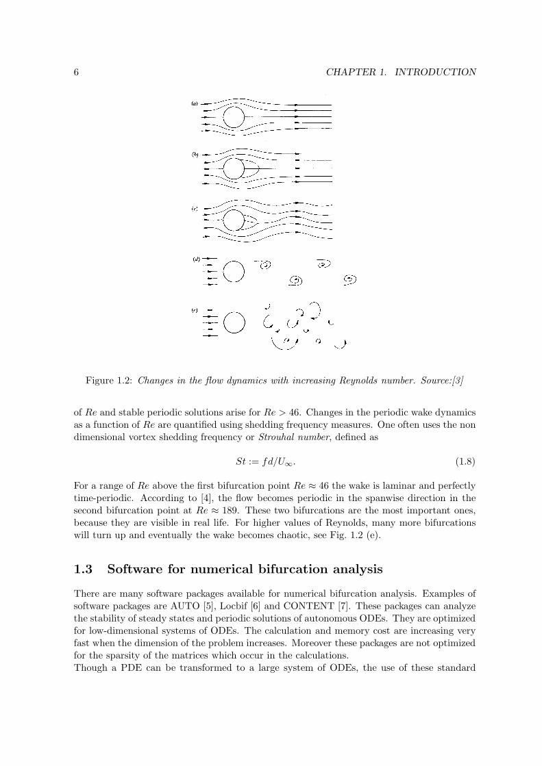
where U∞ denotes the flow velocity far from the cylinder, d is the cylinder-diameter and ν isthe kinematic viscosity. In our case the U∞ = 1 at the inflow boundary. When this Reynoldsnumber is increasing the behavior of the flow, affected by a disturbance, in the cylinder wakechanges. In Fig. 1.2 (taken from [3]) it is illustrated how the flow changes. At a very lowReynolds number the flow is laminar, steady and does not separate from the cylinder (a).When 6 < Re < 46 the flow separates from the cylinder but it is still steady and laminar (b).At Re > 46 the flow becomes time-periodic with the wake oscillating in space (c) and (d).The flow in figure (d) is called the “Von Karman vortex street”. This behavior is still twodimensional with no velocity in the spanwise direction z. After some bifurcations the flowbecomes turbulent (e) and the behavior is fully three dimensional. The Reynolds number Reis the natural branching parameter in this bifurcation problem.
The critical value of Re ≈ 46 marks the transition from stationary solutions to time-periodicsolutions as shown in Fig. 1.2(c)(d). This transition is called a supercritical Hopf bifurcation,because stable stationary solutions become unstable stationary solutions at this critical value
6 CHAPTER 1. INTRODUCTION
Figure 1.2: Changes in the flow dynamics with increasing Reynolds number. Source:[3]
of Re and stable periodic solutions arise for Re > 46. Changes in the periodic wake dynamicsas a function of Re are quantified using shedding frequency measures. One often uses the nondimensional vortex shedding frequency or Strouhal number, defined as
St := fd/U∞. (1.8)
For a range of Re above the first bifurcation point Re ≈ 46 the wake is laminar and perfectlytime-periodic. According to [4], the flow becomes periodic in the spanwise direction in thesecond bifurcation point at Re ≈ 189. These two bifurcations are the most important ones,because they are visible in real life. For higher values of Reynolds, many more bifurcationswill turn up and eventually the wake becomes chaotic, see Fig. 1.2 (e).
1.3 Software for numerical bifurcation analysis
There are many software packages available for numerical bifurcation analysis. Examples ofsoftware packages are AUTO [5], Locbif [6] and CONTENT [7]. These packages can analyzethe stability of steady states and periodic solutions of autonomous ODEs. They are optimizedfor low-dimensional systems of ODEs. The calculation and memory cost are increasing veryfast when the dimension of the problem increases. Moreover these packages are not optimizedfor the sparsity of the matrices which occur in the calculations.Though a PDE can be transformed to a large system of ODEs, the use of these standard

1.3. SOFTWARE FOR NUMERICAL BIFURCATION ANALYSIS 7
packages often becomes prohibitively expensive. There are just a few software packages avail-able for continuation and bifurcation analysis of solutions of PDEs. A well known packageis PLTMG [8]. But this package is not capable of analyzing the stability of the calculatedsolution and can not detect some types of bifurcation points like the Hopf bifurcation. K.Lustdeveloped a continuation software package PDEcont [1]. This is a time stepper-based contin-uation code for large systems. PDEcont can analyze the stability of steady-states as well asperiodic solutions.

8 CHAPTER 1. INTRODUCTION

Chapter 2
The theory
Now we need some mathematical theory about stability. We have to investigate the stabilityof isolated steady states and isolated periodic solutions. In this project one of the goals is todo a stability analysis over a range of Reynolds numbers and try to find the first instability atRe ≈ 46. In this chapter we give theory to determine the stability information correspondingto the solutions and a technique to compute solutions in a range of Reynolds numbers. Withthe stability information we can locate bifurcation points like the Hopf bifurcation.
2.1 Linear stability
Many physical models can be written as a system of autonomous ordinary differential equa-tions (ODEs)
dy
dt= f(y, γ) (2.1)
where f : Rn × R → R
n. γ ∈ R is a parameter. Let y∗ be a steady state or a periodicsolution (y∗(t)) of (2.1). Assume we apply a small perturbation u′
0 at t = t0. To investigatethe evolution of the perturbation in time, we substitute the perturbed solution y∗(t) + u′(t)in (2.1). Using a first order Taylor expansion of f(y∗ + u′, γ), we obtain the equation
du′(t)
dt= fy(y
∗(t); γ)u′(t), u′(0) = u′0 (2.2)
for the linear evolution of the perturbation u′(t) in time. The matrix fy(y∗(t); γ) ∈ R
n×n
operates on the perturbation u′(t) which means this matrix is important for determiningwhether a solution is stable or not. The solution u′(t) of (2.2) is
u′(t) = eR t
0fy(y∗(τ);γ)dτ u′
0. (2.3)
In our flow problem we have to deal with two types of solutions, namely the steady state y∗
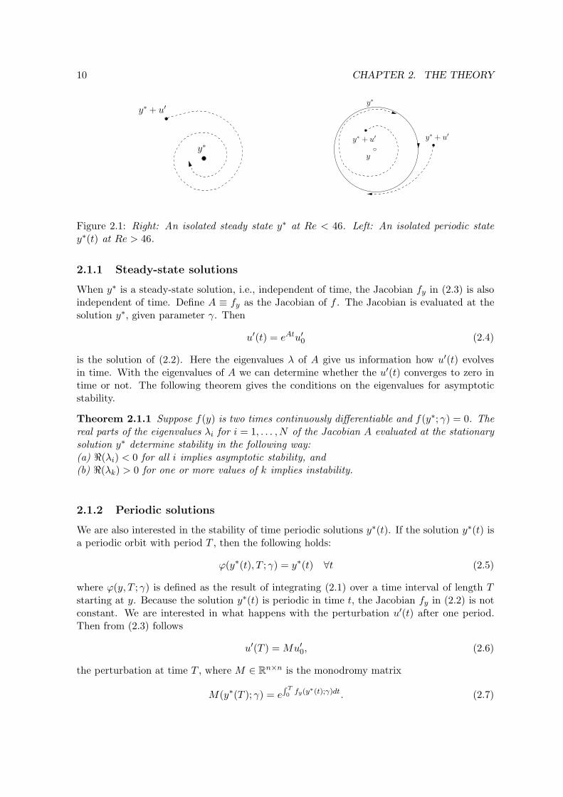
and the periodic solution y∗(t). The meaning of these solutions y∗ and y∗(t) is illustrated inFig. 2.1. When a perturbation u′
0 to y∗ converges to zero in time, y∗ is called asymptoticallystable. In the right figure there is also an unstable steady solution, marked with ◦. In ourflow problem described in Section 1.2, we saw that at Re ≈ 46 a transition takes place froma steady state to a time periodic state. The figure on the left illustrates the situation forRe < 46 and on the right the situation for Re > 46.
9
10 CHAPTER 2. THE THEORY
y∗
y∗ + u′
y∗ + u′ y∗ + u′
y∗
y
Figure 2.1: Right: An isolated steady state y∗ at Re < 46. Left: An isolated periodic statey∗(t) at Re > 46.
2.1.1 Steady-state solutions
When y∗ is a steady-state solution, i.e., independent of time, the Jacobian fy in (2.3) is alsoindependent of time. Define A ≡ fy as the Jacobian of f . The Jacobian is evaluated at thesolution y∗, given parameter γ. Then
u′(t) = eAtu′0 (2.4)
is the solution of (2.2). Here the eigenvalues λ of A give us information how u′(t) evolvesin time. With the eigenvalues of A we can determine whether the u′(t) converges to zero intime or not. The following theorem gives the conditions on the eigenvalues for asymptoticstability.
Theorem 2.1.1 Suppose f(y) is two times continuously differentiable and f(y∗; γ) = 0. Thereal parts of the eigenvalues λi for i = 1, . . . , N of the Jacobian A evaluated at the stationarysolution y∗ determine stability in the following way:(a) <(λi) < 0 for all i implies asymptotic stability, and(b) <(λk) > 0 for one or more values of k implies instability.
2.1.2 Periodic solutions
We are also interested in the stability of time periodic solutions y∗(t). If the solution y∗(t) isa periodic orbit with period T , then the following holds:
ϕ(y∗(t), T ; γ) = y∗(t) ∀t (2.5)
where ϕ(y, T ; γ) is defined as the result of integrating (2.1) over a time interval of length Tstarting at y. Because the solution y∗(t) is periodic in time t, the Jacobian fy in (2.2) is notconstant. We are interested in what happens with the perturbation u′(t) after one period.Then from (2.3) follows
u′(T ) = Mu′0, (2.6)
the perturbation at time T , where M ∈ Rn×n is the monodromy matrix
M(y∗(T ); γ) = eR T
0fy(y∗(t);γ)dt. (2.7)

2.1. LINEAR STABILITY 11
The eigenvalues of M give us the information about the evolution of u′.
The monodromy matrix can also be derived differently. Say ϕ(y0, τ ; γ) is a solution of (2.1).Thus
∂ϕ(y0, τ ; γ)
∂τ= f(ϕ(y0, τ ; γ), γ). (2.8)
Differentiating this with respect to y0 gives us the matrix differential equation
∂
∂τ
∂ϕ
∂y0
∣
∣
∣
∣
(y0,τ,γ)
=∂f
∂y
∣
∣
∣
∣
(ϕ(y0,τ,γ),γ)
∂ϕ
∂y0
∣
∣
∣
∣
(y0,τ,γ)
(2.9)
with initial condition
∂ϕ
∂y0
∣
∣
∣
∣
(y0,0,γ)
= I. (2.10)
The solution at time T of the differential equation (2.9) is
∂ϕ
∂y0
∣
∣
∣
∣
(y0,T,γ)
= eR T
0fy(ϕ(y0,τ ;γ),γ)dτ = M(y0, T, γ) (2.11)
where M is again the monodromy matrix. Here M is written as the derivative of ϕ withrespect to the state vector y. The eigenvalues µ of M are called Floquet multipliers. µ isdefined as
µ = eσT , (2.12)
where σ is called the Floquet exponent and plays the same role as the eigenvalues λ of A.The eigenvectors of M are called Floquet modes. We give a theorem about the properties ofthe Floquet multipliers for stability.
Theorem 2.1.2 Let (y∗, T ; γ) determine a periodic solution of (2.1). Let M be the mon-odromy matrix for this orbit. Let µ1 = 1, µ2, . . . , µN be the N eigenvalues of M .Then:(a) The periodic orbit determined by (y∗, T ; γ) is asymptotically stable if |µi| < 1, i = 2, . . . , N .(b) The periodic orbit determined by (y∗, T ; γ) is unstable if |µi| > 1 for at least one value of i.
A bifurcation occurs if a Floquet multiplier crosses the unit circle. There are three possiblescenarios: Floquet multiplier µi = 1, µi = −1 and µi = e±iσ [1].
If a solution y∗ at a parameter value γ from system (2.1) is stable and γ is close to γc,then a small perturbation in the parameter γ can lead to another solution y. In our flowproblem, when we are close to Re = 46 a small perturbation can lead to a transition to aperiodic solution y∗(t). Two complex conjugate eigenvalues cross the imaginairy axis and thereal part becomes positive. A Hopf bifurcation occurs.At the Hopf bifurcation the two complex conjugate eigenvalues are λ = ±βi, where β denotesthe initial angular velocity of the periodic solution. Thus β = 2πf with f the frequency.

12 CHAPTER 2. THE THEORY
From the definition of the Floquet multiplier (2.12) the complex conjugate eigenvalues λ aremapped to 1 as
e±βiT = e±2πiT−1T = e±2πi = 1. (2.13)
This means that two Floquet multipliers equal to one marks the beginning of the periodicregime.
Definition 2.1.1 A bifurcation from a branch of equilibria to a branch of periodic oscillationsis called a Hopf bifurcation.
This happens in our system at Re ≈ 46. At Re ≈ 189 there is a bifurcation to a threedimensional state. Unfortunately we can not find this instability, because we use the DNScode in a two dimensional mode.
2.2 Continuation
Now we know how to calculate the stability of solutions y∗ and are able to locate bifurcationsby computing the dominant eigenvalue of Floquet multiplier. We have to determine therightmost eigenvalues of A or the largest in modulus eigenvalues of M to see whether asolution is stable or not. Of course we are interested in the whole branch of stable solutionsand the values of our branching parameter γ where stability is lost.With the technique of continuation we can calculate a branch of stable and unstable solutions.The continuation process contains two steps. First a predictor step, where a new point onthe branch is predicted and second the corrector step where the predicted point is refined toa new point on the branch.
2.2.1 The predictor
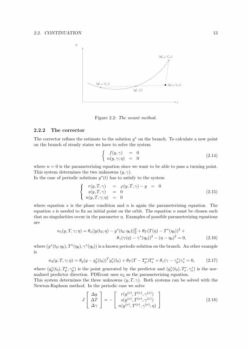
The predictor predicts the next point on the branch based on already known points. PDE-cont predicts new points by means of polynomial extrapolation using already known points(y, γ), where a point consists of a state y at a corresponding value of γ. In PDEcont a linearextrapolation method is used, called the secant predictor. In Fig. 2.2 the main idea is shown.First the search direction is computed based on known points. Then a parameter step istaken in that direction.However, a good continuation code does not parameterize the state vector y with the branch-ing parameter γ. When the state vector is parameterized by γ, the continuation code getproblems when the tangent to the curve y(γ) becomes vertical, i.e. a turning point occurs.So, good continuation codes use a new parameter η such that (y(η), γ(η)). The secant methodneeds the current point (y∗i , γ
∗i ) and the previous point (y∗i−1, γ
∗i−1) to compute a search di-
rection an takes a parameter step ∆η. After the prediction, the estimate ( ˆyi+1, ˆγi+1) of thenext solution must be refined to (y∗i+1, γ
∗i+1). (see Fig. 2.2) This is done by the corrector.
2.2. CONTINUATION 13
γ
(y∗i−1, γ∗i−1)
(y∗i+1, γ∗i+1)
( ˆyi+1, ˆγi+1)
y
(y∗i , γ∗i )
Figure 2.2: The secant method.
2.2.2 The corrector
The corrector refines the estimate to the solution y∗ on the branch. To calculate a new pointon the branch of steady states we have to solve the system
{
f(y, γ) = 0n(y, γ; η) = 0
(2.14)
where n = 0 is the parameterizing equation since we want to be able to pass a turning point.This system determines the two unknowns (y, γ).In the case of periodic solutions y∗(t) has to satisfy to the system
r(y, T, γ) = ϕ(y, T, γ) − y = 0s(y, T, γ) = 0
n(y, T, γ; η) = 0(2.15)
where equation s is the phase condition and n is again the parameterizing equation. Theequation s is needed to fix an initial point on the orbit. The equation n must be chosen suchthat no singularities occur in the parameter η. Examples of possible parameterizing equationsare
n1(y, T, γ; η) = θx||y(t0; η) − y∗(t0; η0)||22 + θT (T (η) − T ∗(η0))
2 +
θγ(γ(η) − γ∗(η0))2 − (η − η0)
2 = 0, (2.16)
where (y∗(t0; η0), T∗(η0), γ
∗(η0)) is a known periodic solution on the branch. An other exampleis
n2(y, T, γ; η) = θy(y − y∗p(t0))T y∗s(t0) + θT (T − T ∗
p )T ∗s + θγ(γ − γ∗
p)γ∗s = 0, (2.17)
where (y∗p(t0), T∗p , γ∗
p) is the point generated by the predictor and (y∗s(t0), T∗s , γ∗
s ) is the nor-malized predictor direction. PDEcont uses n2 as the parameterizing equation.This system determines the three unknowns (y, T, γ). Both systems can be solved with theNewton-Raphson method. In the periodic case we solve
J
∆y∆T∆γ
= −
r(y(ν), T (ν), γ(ν))
s(y(ν), T (ν), γ(ν))
n(y(ν), T (ν), γ(ν); η)
(2.18)
14 CHAPTER 2. THE THEORY
where J is the Jacobian matrix
J =
∂r(y(ν),T (ν),γ(ν))∂y
∂r(y(ν),T (ν),γ(ν))∂T
∂r(y(ν),T (ν),γ(ν))∂γ
∂s(y(ν),T (ν),γ(ν))∂y
∂s(y(ν),T (ν),γ(ν))∂T
∂s(y(ν),T (ν),γ(ν))∂γ
∂n(y(ν),T (ν),γ(ν))∂y
∂n(y(ν),T (ν),γ(ν))∂T
∂n(y(ν),T (ν),γ(ν))∂γ
, (2.19)
followed by the update
y(ν+1) = y(ν) + ∆y, (2.20)
T (ν+1) = T (ν) + ∆T, (2.21)
γ(ν+1) = γ(ν) + ∆γ, (2.22)
where we use (y(0), T (0), γ(0)) from the predictor as starting point. In the Jacobian matrix(2.19) we see derivatives of r(y, T, γ) = ϕ(y, T, γ) − y with respect to y, T and γ. In the firstderivative,
∂r(y, T, γ)
∂y=
∂ϕ(y, T, γ)
∂y− I = M − I (2.23)
we recognize the monodromy matrix M (2.11) explained in the previous section. This matrixis also needed for the determination of the stability.
2.3 The stability results from literature
There is already a lot of literature about this particular stability problem. Therefore twoarticles, which are referenced in many studies about this flow problem, are used for the mainidea. The first instability at Re ≈ 46 was studied by Jackson in [3]. This is a bifurcation from atwo dimensional to a two dimensional state and hence it can be analyzed in a two dimensionaldomain. The second instability, at Re ≈ 189, is a bifurcation to a three dimensional state.This bifurcation was studied by Barkley [9]. We will not calculate this instability in thisproject, but we can see how Barkley used a flow solver to find this instability.
2.3.1 First instability by Jackson
The first instability is found by Jackson [3]. At Re < 46 the solution is a stable steady-state.At Re ≈ 46 a Hopf bifurcation occurs and the flow becomes periodic in time. The frequencyof the periodic solution is quantified by the Strouhal number (1.8).After space discretisation of the Navier-Stokes equations (1.1) the system can be rewritten as
Bdy
dt= f(y,Re), (2.24)
where f : Rn × R → R
n. B is a singular matrix, because the continuity equation is timeindependent. Jackson was interested in the value of Reynolds where the Hopf bifurcationoccurs. He calculated the solutions y∗ and the the corresponding eigenvalues for the stabilityanalysis. He was interested in the equilibria y∗ which are solutions of
f(y;Re) = 0. (2.25)
2.3. THE STABILITY RESULTS FROM LITERATURE 15
At the Hopf bifurcation point a pair of complex conjugate eigenvalues crosses the imaginaryaxis. Jackson used extended-system techniques which give accurate results for the criticalReynolds and Strouhal number. He used the following extended system:
f(y;Re) = 0,fyξr + ωBξi = 0,fyξi − ωBξr = 0,
(ek)T · ξr = 0,(ek)T · ξi = 1,
where the subscripts r and i denote the real and imaginary part of the eigenvector ξ. Thisextended system determines a Hopf bifurcation point, the real and imaginary parts of thebifurcating eigenvector and the corresponding angular frequency ω and Reynolds number Re.The complex eigenvalues can be traced with the continuation technique.This approach is much cheaper than time-dependent calculations for determining these quan-tities. However, this technique does not give directly the time-dependent behavior at valuesgreater than the critical Reynolds number Re ≈ 46.
2.3.2 Second instability by Barkley
The second instability at Re ≈ 189, which corresponds with three-dimensional flow, has beenfound by Barkley and Henderson [9]. Because three-dimensional simulations are very expen-sive, a two dimensional flow is calculated. With an artificial periodic flow in the spanwisedirection z the second instability can be found. A two dimensional periodic solution y∗(t) isobtained with direct numerical simulation from (1.1). The techniques Barkley used to calcu-late the periodic solutions are discussed in detail in Henderson and Karniadakis [10]. For thecontinuation of the solution at different Reynolds numbers Barkley used a shooting technique[1]. For the stability analysis a three-dimensional perturbation u
′(x, y, z, t) is added to theperiodic solution y∗(t). The evolution of the perturbation u′(t) is described by a linearizedNavier-Stokes equation.The system is homogeneous in the spanwise direction z and the perturbation can be decom-posed in space by a Fourier transform
u′(x, y, z, t) =
∫
∞
−∞
u′
β(x, y, t)eiβzdβ. (2.26)
The decomposition of the perturbed pressure p′ is similar. In the linearized equation themodes with different wave numbers β do not couple. Now take for example a perturbation
u′(x, y, z, t) = (u′
β(x, y, t) cos βz, v′β(x, y, t) cos βz,w′β(x, y, t) sin βz),
p′(x, y, z, t) = p′β(x, y, t) cos βz. (2.27)
This perturbation will remain in this form under M(y∗;Re) and hence every wave num-ber β can be considered separately. After substituting the chosen perturbations in equation(2.2) the unknown components (u′
β , v′β, w′β) and pressure p′β from (2.27) can be computed.
These unknowns are functions of x, y and t. What follows is an extra parameter β, the wavenumber. The main objective of Barkley is to determine the precise range of Re and β forwhich a perturbation of the periodic solution grows. Via Floquet analysis the stability of thetime-dependent periodic solution y∗(t) is determined. The method used to find the Floquet
16 CHAPTER 2. THE THEORY
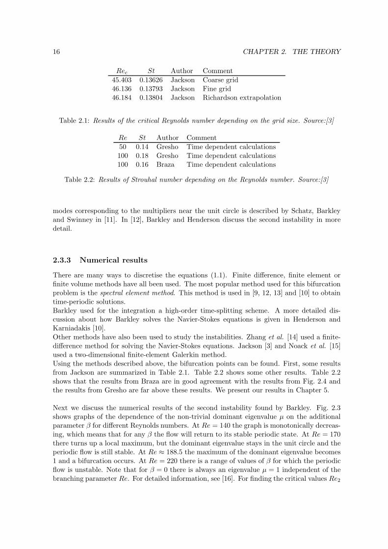
Rec St Author Comment
45.403 0.13626 Jackson Coarse grid46.136 0.13793 Jackson Fine grid46.184 0.13804 Jackson Richardson extrapolation
Table 2.1: Results of the critical Reynolds number depending on the grid size. Source:[3]
Re St Author Comment
50 0.14 Gresho Time dependent calculations100 0.18 Gresho Time dependent calculations100 0.16 Braza Time dependent calculations
Table 2.2: Results of Strouhal number depending on the Reynolds number. Source:[3]
modes corresponding to the multipliers near the unit circle is described by Schatz, Barkleyand Swinney in [11]. In [12], Barkley and Henderson discuss the second instability in moredetail.
2.3.3 Numerical results
There are many ways to discretise the equations (1.1). Finite difference, finite element orfinite volume methods have all been used. The most popular method used for this bifurcationproblem is the spectral element method. This method is used in [9, 12, 13] and [10] to obtaintime-periodic solutions.Barkley used for the integration a high-order time-splitting scheme. A more detailed dis-cussion about how Barkley solves the Navier-Stokes equations is given in Henderson andKarniadakis [10].Other methods have also been used to study the instabilities. Zhang et al. [14] used a finite-difference method for solving the Navier-Stokes equations. Jackson [3] and Noack et al. [15]used a two-dimensional finite-element Galerkin method.Using the methods described above, the bifurcation points can be found. First, some resultsfrom Jackson are summarized in Table 2.1. Table 2.2 shows some other results. Table 2.2shows that the results from Braza are in good agreement with the results from Fig. 2.4 andthe results from Gresho are far above these results. We present our results in Chapter 5.
Next we discuss the numerical results of the second instability found by Barkley. Fig. 2.3shows graphs of the dependence of the non-trivial dominant eigenvalue µ on the additionalparameter β for different Reynolds numbers. At Re = 140 the graph is monotonically decreas-ing, which means that for any β the flow will return to its stable periodic state. At Re = 170there turns up a local maximum, but the dominant eigenvalue stays in the unit circle and theperiodic flow is still stable. At Re ≈ 188.5 the maximum of the dominant eigenvalue becomes1 and a bifurcation occurs. At Re = 220 there is a range of values of β for which the periodicflow is unstable. Note that for β = 0 there is always an eigenvalue µ = 1 independent of thebranching parameter Re. For detailed information, see [16]. For finding the critical values Re2

2.3. THE STABILITY RESULTS FROM LITERATURE 17
Rec βc Author Comment
188.5 1.585 Barkley Spectral element170 1.75 Konig, Noack and Eckelmann Galerkin
Table 2.3: Results with different methods.
and β, stability computations are performed at Re = 187 and Re = 190 for β = 1.4, 1.5, 1.6and 1.7. With two-dimensional fit the critical values are Re = 188.6 and β = 1.584. Atthis value the dominant eigenvalue or Floquet multiplier leaves the unit circle and the flowbecomes fully three-dimensional. Table 2.3 shows the two result from Barkley, Noack, Konig
Figure 2.3: Parameter dependence of the dominant Floquet multiplier on the spanwise wavenumber β Source:[9]
and Eckelmann [15]. Konig, Noack and Eckelmann used in their Galerkin projection methoda much lower number of grid elements than Barkley. The experimental results for the secondinstability were very inaccurate, so they were satisfied with their numerical results at thattime.
To find an accurate result for the second instability in the third dimension, the mesh size ofthe grid has influence on the critical Reynolds number. The mesh dependence of the periodicsolutions and the stability calculation, is discussed in [9]. In [4] different sub-domains of thesolution are used to analyze the Floquet multipliers.
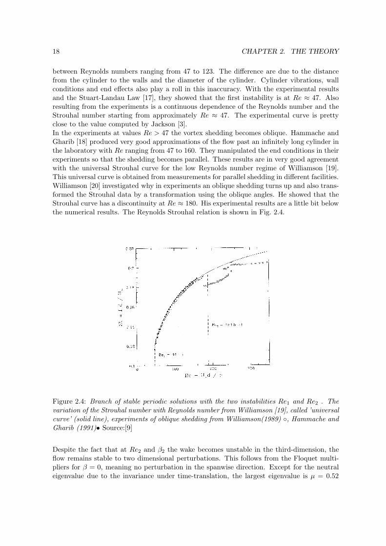
In Fig.2.4 the main results are shown. The two important critical values Re1 ≈ 46 andRe2 ≈ 188.5 and the branch of stable periodic solutions are depicted.To verify the numerical results, experimental results are needed. It is very difficult to findthe two important instabilities in experiments. What can be found is the branch of periodicsolutions, or equivalently, the relation between the Strouhal number and the Reynolds num-ber. A lot of experiments have been done by Mathis, Provensal and Boyer [17]. They didexperiments with Reynolds numbers ranging from 40 to 300. The first instability is found
18 CHAPTER 2. THE THEORY
between Reynolds numbers ranging from 47 to 123. The difference are due to the distancefrom the cylinder to the walls and the diameter of the cylinder. Cylinder vibrations, wallconditions and end effects also play a roll in this inaccuracy. With the experimental resultsand the Stuart-Landau Law [17], they showed that the first instability is at Re ≈ 47. Alsoresulting from the experiments is a continuous dependence of the Reynolds number and theStrouhal number starting from approximately Re ≈ 47. The experimental curve is prettyclose to the value computed by Jackson [3].In the experiments at values Re > 47 the vortex shedding becomes oblique. Hammache andGharib [18] produced very good approximations of the flow past an infinitely long cylinder inthe laboratory with Re ranging from 47 to 160. They manipulated the end conditions in theirexperiments so that the shedding becomes parallel. These results are in very good agreementwith the universal Strouhal curve for the low Reynolds number regime of Williamson [19].This universal curve is obtained from measurements for parallel shedding in different facilities.Williamson [20] investigated why in experiments an oblique shedding turns up and also trans-formed the Strouhal data by a transformation using the oblique angles. He showed that theStrouhal curve has a discontinuity at Re ≈ 180. His experimental results are a little bit belowthe numerical results. The Reynolds Strouhal relation is shown in Fig. 2.4.
Figure 2.4: Branch of stable periodic solutions with the two instabilities Re1 and Re2 . Thevariation of the Strouhal number with Reynolds number from Williamson [19], called ’universalcurve’ (solid line), experiments of oblique shedding from Williamson(1989) ◦, Hammache andGharib (1991)• Source:[9]
Despite the fact that at Re2 and β2 the wake becomes unstable in the third-dimension, theflow remains stable to two dimensional perturbations. This follows from the Floquet multi-pliers for β = 0, meaning no perturbation in the spanwise direction. Except for the neutraleigenvalue due to the invariance under time-translation, the largest eigenvalue is µ = 0.52

2.3. THE STABILITY RESULTS FROM LITERATURE 19
which means that the perturbation is decreasing by factor of about two per period. Thiseigenvalue stays in the unit-circle until at least Re = 250, the end of Barkleys computationswhich means that the two-dimensional flow is stable under two dimensional perturbations forRe ≤ 250. Noack, Konig and Eckelmann [15] confirmed that all the eigenvalues which are as-sociated with the two-dimensional Floquet modes stay in the unit circle for Re ≈ 50 up to 500.

20 CHAPTER 2. THE THEORY
Chapter 3
Numerical methods
We already introduced the codes used in this project in Section 1.3. Now we explain how wereached our first goal, the numerical bifurcation analysis of our flow problem. We use DNSfor time integration and PDEcont for calculating the branches of solutions y∗ depending ofRe. In this chapter we describe both codes in some more detail. We want to know how thesecodes work, because these codes have to work together. Therefore we need information aboutthe in- and output of both programs. There are different ways to couple both codes. Wedecided to couple the codes by exchanging data by files. This is probably the easiest way todo this. We come back to this topic later in Chapter 4.We also describe some numerical tools the codes use and how the computations are done.We know that there are two methods for doing a numerical bifurcation analysis: repeatedsimulations and continuation. Both ways are done in this project. We will see that the firstmethod is not very efficient. For the first method only the DNS code is used to simulate theflow from a certain initial condition y0 = y(t0) in time. In this way we can look how thebehavior of the flow changes when the physical parameter Re is changing. The results arepresented in Section 5.1.For the second method we use PDEcont in combination with DNS. In Chapter 4 we showhow this is realized. The results are presented in Chapter 5.
3.1 DNS
3.1.1 What does DNS do?
On a predefined domain DNS gives us ϕ(y0, T ;Re), the time integration over the time intervalT starting from the initial state y0 at a given Reynolds number Re. From the introductionwe already know that we have two regimes in our flow problem: A steady state regime forRe . 46 and a periodic regime for Re & 46 (see Fig. 2.1). In Fig. 3.1 we show some resultsfrom DNS started with values of Re in a different regime.
21
22 CHAPTER 3. NUMERICAL METHODS
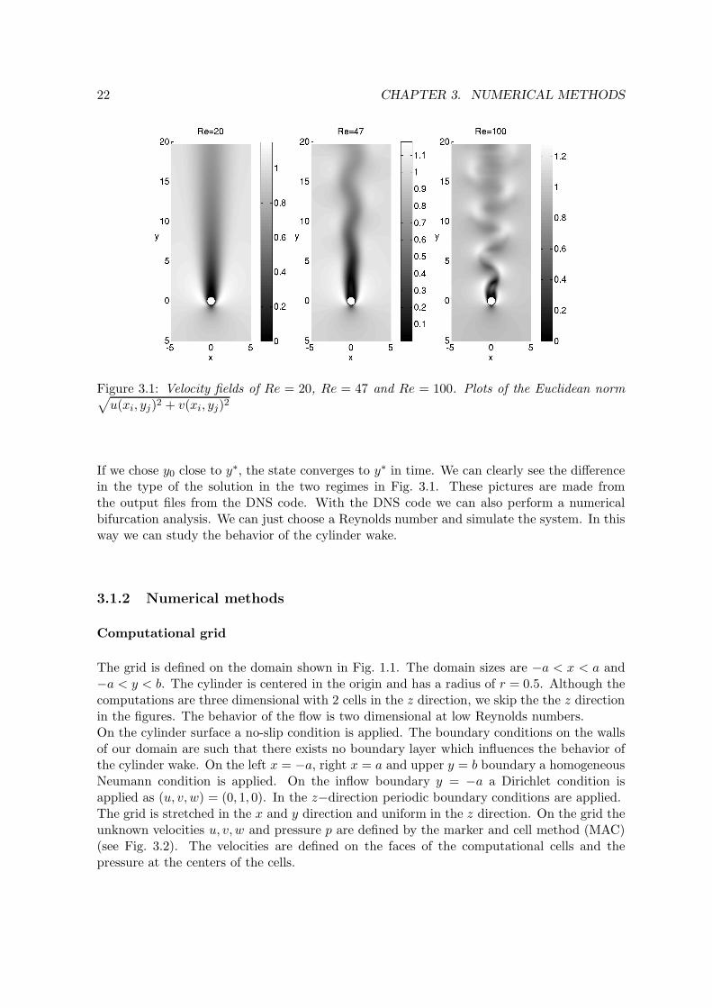
Figure 3.1: Velocity fields of Re = 20, Re = 47 and Re = 100. Plots of the Euclidean norm√
u(xi, yj)2 + v(xi, yj)2
If we chose y0 close to y∗, the state converges to y∗ in time. We can clearly see the differencein the type of the solution in the two regimes in Fig. 3.1. These pictures are made fromthe output files from the DNS code. With the DNS code we can also perform a numericalbifurcation analysis. We can just choose a Reynolds number and simulate the system. In thisway we can study the behavior of the cylinder wake.
3.1.2 Numerical methods
Computational grid
The grid is defined on the domain shown in Fig. 1.1. The domain sizes are −a < x < a and−a < y < b. The cylinder is centered in the origin and has a radius of r = 0.5. Although thecomputations are three dimensional with 2 cells in the z direction, we skip the the z directionin the figures. The behavior of the flow is two dimensional at low Reynolds numbers.On the cylinder surface a no-slip condition is applied. The boundary conditions on the wallsof our domain are such that there exists no boundary layer which influences the behavior ofthe cylinder wake. On the left x = −a, right x = a and upper y = b boundary a homogeneousNeumann condition is applied. On the inflow boundary y = −a a Dirichlet condition isapplied as (u, v,w) = (0, 1, 0). In the z−direction periodic boundary conditions are applied.The grid is stretched in the x and y direction and uniform in the z direction. On the grid theunknown velocities u, v,w and pressure p are defined by the marker and cell method (MAC)(see Fig. 3.2). The velocities are defined on the faces of the computational cells and thepressure at the centers of the cells.

3.1. DNS 23
p
ppp
p
y
x
u u
u u u u
u uv
v
v
v
v
v
v
v
hx
hypw peuw uc ue
un
us
vx
vn
Figure 3.2: Left: Locations of the pressure p and velocity components u, v. Note that the cellsare not necessarily squares. They may be stretched in one or more directions. Right: Thesolid square is the control cell around uc.
Spatial discretization
For the spatial discretization a finite-volume method is applied. The discretization is basedon the conservation of the physical quantities u, v and uses control cells around the unknownsu, v; see right picture in Fig. 3.2. In the control cells both conservation of mass and impulseis required. The convective flux −u(u · n) and diffusive flux through the control cells arediscretised by a second order symmetry-preserving method [2]. In the right figure in Fig. 3.2the control cell K for velocity uc is shown.
Time integration
The time integration uses a second-order Adams-Bashforth method. Herefore, first the solu-tion at time levels n and n − 1 are extrapolated to
un+ 1
2 =3
2u
n −1
2u
n−1. (3.1)
The extrapolated value is used to calculate the convective and diffusive fluxes in the controlcells of u, v and w. Next, the velocity field u
n is updated by integration over one time step
u∗ = u
n + δt(convective + diffusive)n+ 12 , (3.2)
indicating that the convective and diffusive term are evaluated with the velocity from (3.1).After the time integration, the updated velocity field u
∗ does not satisfy ∇ · u∗ = 0. We usethe pressure equation to fix this.
Pressure equation
To compute the velocity field un+1 we still have to add the pressure gradient
un+1 = u
∗ − δt∇pn+1, (3.3)
24 CHAPTER 3. NUMERICAL METHODS
where u∗ has been computed by (3.2). Since we want ∇ ·nn+1 = 0, the pressure pn+1 can be
solved from the equation
∇ · (un − dt∇pn+1) = 0 ⇒
∇2pn+1 =1
dt∇ · un. (3.4)
The pressure equation (3.4) is solved with ICCG in the spectral space using fast Fouriertransformation (FFT). The ICCG method is an advanced Conjugate Gradient method (CG)with an incomplete Cholesky factorization as pre-conditioner [21]. With the pressure from(3.4) we can calculate the new state u
n+1 with (3.3).
3.1.3 DNS interface
The DNS code needs a lot of information. First of all, to work properly, it needs someinformation to configure the numerical methods discussed in previous section. The propertiesof the time integration, convergence criteria for the Poisson solver and order of discretizationare needed. Furthermore it needs settings about the size of the calculation domain, thenumber of cells and the boundary conditions. There are also some problem related settings:the Reynolds number Re, time step δt and the number of time steps nt. The product of thelatter two specifies the time integration interval. And finally some output settings determiningthe storage of the state vector at every time interval.When starting the DNS code, the user can choose to start with an initial state vector. Whenthere is no initial state vector defined, DNS starts computing the flow with a zero state vector.In our project, the DNS code always has to start with a given state vector.
3.2 PDEcont
3.2.1 What does PDEcont do?
PDEcont computes branches of solutions y of a physical system and the corresponding sta-bility information with the theory described in chapter 2. It uses a Newton-based singleshooting technique combined with a Picard iteration process. With PDecont we can get anoverview of all the asymptotic solutions y, i.e., stable and unstable solutions in a certain rangeof the physical parameter γ. The critical values γc, where certain instabilities occurs, can bealso found. Due to this continuation code we get a good understanding of the behavior of aphysical system in certain conditions. With this kind of research, we hope to avoid eventslike the collapse of the Tacoma Narrows suspension bridge.To understand how PDEcont works we continue with the numerical methods used by PDE-cont.
3.2.2 Numerical methods
The Floquet multipliers µ of the monodromy matrix M characterize the stability of a periodicsolution y∗(t). It is too expensive to compute all the Floquet multipliers and moreover, mostof these multipliers aren’t even interesting.A property of the physical system we investigate is the fact that most multipliers are closeto zero and thus are not able to cause any instability of y∗(t). The instability is caused by
3.2. PDECONT 25
those multipliers which are close to the unit circle. PDEcont computes only these dominantmultipliers of M . To define the most dominant Floquet multipliers of the system, PDEcontuses the following assumption.
Assumption 3.2.1 Let y∗ = (y∗(t0), T∗) denote an isolated solution to (2.15), and let B be
a small neighborhood of y∗(t). Let M(y) = ∂ϕ∂y(t0)(y) for y ∈ B and denote its eigenvalues by
µi, i = 1, ..., N . Assume that for all y ∈ B precisely p eigenvalues lie outside the disk
Cρ = {|z| < ρ}, 0 < ρ < 1 (3.5)
and no eigenvalues has modulus ρ; i.e., for all y ∈ B
|µ1| ≥ |µ2| ≥ · · · ≥ |µp| > ρ > |µp+1|, · · · , |µN |. (3.6)
The dominant Floquet multipliers defined by this assumption and the corresponding eigenvec-tors are computed using an orthogonal subspace iteration technique. PDEcont computes thebasis for the p-dimensional subspace U ⊂ R
N of the generalized eigenvectors corresponding toµ1, · · · , µp. Let the column vectors of Vp ∈ R
N×p define an orthonormal basis for the subspaceU of R
N and the column vectors of Vq ∈ RN×(N−p) = R
N×q define an orthonormal basis forU⊥, the orthogonal complement of U in R
N . These matrices Vp and Vq can be computedby the real Schur factorization of M . Note that Vq is a huge matrix and we do not want tocompute this matrix in the final algorithm.Now we can construct orthogonal projectors P and Q of R
N onto the subspaces U and U⊥
respectively as
P := VpVTp ,
Q := VqVTq = IN − VpV
Tp . (3.7)
Now for any y(t0) ∈ RN there exists a unique decomposition
y(t0) = Vpp + Vq q = Py(t0) + Qy(t0). (3.8)
Consider the system (2.18),
M − I bT bγ
cTs ds,T ds,γ
cTn dn,T dn,γ
∆y∆T∆γ
= −
rsn
, (3.9)
where we abbreviated the derivatives in the iteration matrix. By multiplying the first Nequations with [Vq Vp]
T and substituting (3.8) into (3.9) we can write the system in terms ofthese matrices Vp and Vq. This gives the possibility to split the system into a q− and a p−dimensional subsystem, where p << q.We also know V T
p Vq = 0p×q, VTq Vp = 0q×p and V T
q MVp = 0, where the latter equation holdssince U is an invariant subspace of M(y(t0), T, γ)). We get the following system:
V Tq MVq − Iq 0 0 V T
q bγ
V Tp MVq V T
p MVp − Ip V Tp bT V T
p bγ
cTs Vq cT
s Vp ds,T ds,γ
cTnVq cT
n Vp dn,T dn,γ
∆q∆p∆T∆γ
= −
V Tq r
V Tp r
sn
. (3.10)
26 CHAPTER 3. NUMERICAL METHODS
From the system (3.10) we can write the q system as
(V Tq MVq − Iq)∆q = −(V T
q r + V qT bγ∆γ). (3.11)
Since (V Tq MVq − Iq) is nonsingular by construction we can transform (3.11) into
∆q = −(V Tq MVq − Iq)
−1(V Tq r + V qT bγ∆γ). (3.12)
We split the ∆q into two components ∆qr and ∆qγ as
∆q = ∆qr + ∆γ∆qγ, (3.13)
and obtain two separate subsystems
(V Tq MVq − Iq)∆qr = −V T
q r and (V Tq MVq − Iq)∆qγ = −V T
q bγ . (3.14)
Each of these subsystems is solved approximately by a Picard iteration scheme. To avoidcomputing the large matrix Vq, we use the projectors P,Q (3.7) by multiplying every iterationstep with Vq. Let b denote either r or bγ . The Picard iteration is
∆q[0] = 0,
∆q[i] = VqVTq M∆q
[i−1]b + VqV
Tq b
= QM∆q[i−1]b + Qb, i = 1, · · · , l,
∆qb = ∆q[l]b
(3.15)
where ∆qb = ∆qr if b = r and ∆qb = ∆qγ if b = bγ . Substituting ∆q into (3.10) and rewritingin terms of the components ∆qr and ∆qγ we get
V Tp MVp − Ip V T
p bT V Tp (bγ + MV T
q ∆qγ)
cTs Vp ds,T ds,γ + cT
c Vq∆qγ
cTnVp dn,T dn,γ + cT
n Vq∆qγ
∆p∆T∆γ
= −
V Tp (r + MVq∆qr)
s + cTs Vq∆qr
n + cTnVq∆qr
.(3.16)
First the two systems (3.14) are solved approximately using Picard iteration (3.15). Then wecompute ∆p,∆T and ∆γ from (3.16) and finally ∆q is computed with (3.13)The nice thing of this approach is that PDEcont computes branches of solutions and alsoreturns stability information at little or no extra cost.
Variable step size
In PDEcont we use a variable step size. It is not safe to fix the step size ∆η, because whenthe step size is too large there is the possibility to jump to another branch or jump over abifurcation point. PDEcont decides how large the step is, the convergence of the Newton-Picard iterations. When the parameter step ∆η in the computed direction is too large, theNewton-Picard step will fail. As a result, half the steplength ∆η will be used. When theNewton-Picard step succeeds, the steplength will grow by a factor. The behavior of thesteplength can be configured by the user. For detailed information see the manual [22].

3.3. WHAT TO DO? 27
3.2.3 PDEcont interface
First of all, to run the PDEcont code a lot of work is required. We can only start PDEcontwhen the system to investigate, is implemented. A lot of settings PDEcont needs are depen-dent on how the user has implemented the system. However PDEcont still needs a lot ofsettings for configuring the solver and the continuation method. Also some settings of thesolution type and branch type are required.The solver has to deal with three iteration processes, namely the Newton-Raphson iteration,orthogonal subspace iteration and the Picard iteration. Every iteration process needs a lot ofsetting as thresholds, convergence criteria, maximum number of iteration steps, etc.Also the continuation method requires a lot of settings. PDEcont uses a variable stepsizemethod. Here settings are needed for minimum, maximum and starting stepsize, some con-stants which have to do with the behavior of the stepsize, the range of the branching parameterγ and the number of branch points to compute in that range. Finally PDEcont needs of coursea starting point (y, T, γ) close to a branch. All the details are in the PDEcont manual [22].
3.3 What to do?
For this project we want to compute the branch of steady-states and periodic solutions andgive an accurate result of the location of the Hopf bifurcation. We have to implementour flow problem into PDEcont and compute the branches in combination with the DNScode. PDEcont is the main program. PDEcont starts the continuation process with a pointxi = (yi, Ti, Rei). As a result PDEcont gives the point on the branch x∗
i = (y∗i , T∗i , Re∗i ). To
find this point x∗i , the solver from PDEcont needs to compute some directional derivatives
and the derivatives with respect to Re and T of ϕ(y, T,Re) at every iteration step. This isexplained in section 2.2. The ϕ is computed by the DNS code. This means that the DNScode needs a y, T and Re. While running, PDEcont gives DNS the y, T and Re. DNS sendsthe results back and PDEcont uses these results to continue the continuation process. Thisexchange of information is very important to couple the codes. In the Fig. 3.3 we give aschematic view of the information exchange.
In the next chapter we describe in detail how this is done.

28 CHAPTER 3. NUMERICAL METHODS
D N S
t
n
o
c
E
D
P
y, T, Re
yi, Ti, Rei
ϕ(yi, Ti, Rei)
y∗, T ∗, Re∗
Figure 3.3: Schematic view of the data exchange between PDEcont and DNS.
Chapter 4
Implementation
From section 3.3 we know that both programs have to work together and that some informa-tion must be exchanged between the codes. Therefore we have to create some communicationroutines and implement them in PDEcont. When PDEcont needs a solution of a time inte-gration it gives the proper information to the DNS code. The DNS code gets the calculationjob from PDEcont and when finished it gives the results back to PDEcont.The communication routines are created with the knowledge we have of the format of the filescontaining Re, T and y. These routines are created specific for this DNS code and cannot beused for other purposes.
4.1 Implementation methods
There are different methods of implementing a system into PDEcont. The implementationmethod is very dependent on the simulation code and the creative powers of the programmer.In this project, we have to find out to what extent the DNS code can be used for timestepper-based bifurcation analysis. We can interpret this again into different implementation methods.We discuss two of them.
4.1.1 Possible methods
Our first idea was to use the DNS code for what it is and do all the necessary data exchangeshown in Fig. 3.3 by ASCII files. The communication routines read and write the data in theproper format. Nothing of the concerning content of the DNS code is skipped or changed.The second possibility is to split up the DNS code in a subroutine that does the initializationsand a subroutine for the time integration and link both routines into PDEcont. The codesare written in different programming languages, namely DNS in Fortran and PDEcont in C.This method requires thus more programming in both languages Fortran and C, but whenfinished, it is probably easier to run and easier to debug. We used the first method and willnot discuss the second method any further.
4.1.2 Our method
We have chosen to exchange the data Re, T and y by files and leave the DNS code for what itis. The method we used makes the implementation and the connection easy, because we don’thave to strip down the DNS code and all the programming work will be in C. This means
29
30 CHAPTER 4. IMPLEMENTATION
the program work is a lot easier compared with the other method we mentioned. Althoughsome small changes in the DNS code are required. These are discussed in Chapter 6. Wethink that the communication between the codes slows down the performance. More of thismethod in our final discussion in Chapter 6.
4.2 Implementation with files
4.2.1 Files for data exchange between PDEcont and DNS
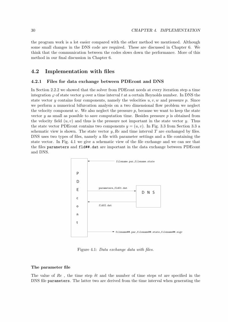
In Section 2.2.2 we showed that the solver from PDEcont needs at every iteration step a timeintegration ϕ of state vector y over a time interval t at a certain Reynolds number. In DNS thestate vector y contains four components, namely the velocities u, v,w and pressure p. Sincewe perform a numerical bifurcation analysis on a two dimensional flow problem we neglectthe velocity component w. We also neglect the pressure p, because we want to keep the statevector y as small as possible to save computation time. Besides pressure p is obtained fromthe velocity field (u, v) and thus is the pressure not important in the state vector y. Thusthe state vector PDEcont contains two components y = (u, v). In Fig. 3.3 from Section 3.3 aschematic view is shown. The state vector y,Re and time interval T are exchanged by files.DNS uses two types of files, namely a file with parameter settings and a file containing thestate vector. In Fig. 4.1 we give a schematic view of the file exchange and we can see thatthe files parameters and fld##.dat are important in the data exchange between PDEcontand DNS.
D N S
t
n
o
c
E
D
P
parameters,fld01.dat
fld02.dat
filename.par,filename.state
filename##.par,filename##.state,filename##.eigv
Figure 4.1: Data exchange data with files.
The parameter file
The value of Re , the time step δt and the number of time steps nt are specified in theDNS file parameters. The latter two are derived from the time interval when generating the
4.2. IMPLEMENTATION WITH FILES 31
parameter file. The file parameters is divided into sections and every section contains somesettings of parameters. An important section is for example
----- Time integration --------------------------
nt = 1398
dt = 4.9956631298147492e-03
beta = 5.0000000000000003e-02
The important parameters from the parameter file are Re, nt, dt, nsf. nsf is easily missedand very important. This value plays an important role in the output of DNS. This parameteris an integer and every nsf time steps the state is stored in the state file. Since we are onlyinterested in the state at time step nt, nsf must be a divisor of nt to store the final state.We take nsf equal to nt, because storing the state every nsf time steps will slow down thecomputations.
The state vector file
Another important file can be found in the dat/ directory of DNS, namely the state filefld##.dat containing the state vector y. The state file fld##.dat contains 3 data elements,namely the time t, the state vector in a matrix with 4 columns (u, v,w, p) at time t andfinally the state in a matrix with 3 columns (u, v,w) at time t − δt, where δt is the timestep defined in the file parameters. The run number ## in the state filename is defined inthe Makefile of DNS. This number specifies the file containing the initial state vector y(t0).Every time integration has a run number and the output files containing the result has therun number ##+1 in the file name. The setting in this file is very important to start withthe file containing the initial state vector. For example, fld01.dat contains the state vectory(t0). As a result DNS generates the file fld02.dat containing the state vector ϕ(y(t0), t;Re).
Somehow PDEcont has to read from and write information to these files. The state vector yand parameters Re, dt, nt are written to the standard input filenames of DNS, fld01.dat andparameters respectively. The resulting state of DNS is always written to the file fld02.dat.We use the same run number for every run, so we don’t need to recompile the code.
4.2.2 Files for initialization and results of PDEcont
PDEcont also uses some files. As a result, PDEcont gives a solution (y∗, T ∗, Re∗) on thebranch with the corresponding stability information of this branch point. To analyze all thebranch points we save every point in files. The names of the files are defined as filename##where the filename is defined by the user through the command line options of PDEcont.The ## is the number of the point on the branch assigned by PDEcont. PDEcont restartsthe numbering from one at every run.To make clear the contents of the files, we defined three types of files: files with the extensions.par, .state and .eigv, containing the parameter settings, the state vector y and the corre-sponding eigenvalues respectively. These files are defined only for the output of PDEcont.(SeeFig. 4.1) It is also possible to restart the continuation process with the output files .par and

32 CHAPTER 4. IMPLEMENTATION
.state.
The .state files contains two data elements, namely the time t and the state y∗(t) =(u∗, v∗, w = 0, p = 0) on the branch. This file is not the same as the state file .dat from DNS.Remember that the state file from DNS contains 3 data elements, namely the time t, the statey(T ) = ϕ(y(t0);Re) containing the four components (u, v,w, p) and the state at y(T − δt)containing three components (u, v,w). These state files are thus not directly useable for DNS.When a branch point is computed, PDEcont stores the state to filename##.state.
The format of the .par files are exactly the same as the format of the parameter file DNS usesand contains exactly the same information. PDEcont starts with a solution y = (y(t0), T,Re)close to the branch, where T =nt∗dt. The corresponding parameter settings of the newbranch point are stored in filename##.par.
Finally, when the next point on the branch is found, the corresponding stability informa-tion is stored in the .eigv file.
We start PDEcont with a point (y, T,Re) close to the branch. PDEcont needs two startingfiles filename.state and filename.par containing y and T,Re respectively. The filename
can be specified by the use in the configuration file of PDEcont. When the next branch pointis found all the necessary information is stored in the files filename## and from the lastcalculated point PDEcont continuous to compute the next branch point.
4.2.3 Implementation of the IO routines
Now we know which files are important and we have seen in Fig. 4.1 that two types of files areused for the data exchange between PDEcont and DNS. We need two routines which are ableto read the files containing the parameter settings and the files containing the state vector.We have to keep in mind that the files fld##.dat and the .state files do not have the sameformat. Note that the format of the .par files and parameters is the same.We also need two routines which are able to write the parameter files and the state files.With these four IO routines PDEcont must be able to read data and change data in thesefiles. We created the routines ReadPar, WritePar, ReadState and WriteState based onthe known format of the parameters and fld##.dat from DNS. The routines are written inC such that they can be implemented in PDEcont. The technical details of these IO routinescan be found in the appendix.
ReadPar
This routine is programmed to read the .par files and the file parameters from DNS. Thesefiles have a fixed format. This routine scans the files for the parameter names Re, nt, dt,
nsf and stores the values of these parameters in memory, such that PDEcont can use thesesettings.
WritePar
When this routine is called, the parameter values of Re, nt, dt, nsf stored in memory arewritten to a .par file or parameters. Because the format is fixed the initial filename.par

4.2. IMPLEMENTATION WITH FILES 33
will be copied, but only the changed parameter values of Re, nt, dt, nsf are overwrittento the new target file. This target file could be a new filename##.par or parameters.
ReadState
This routine has two modes, namely reading a DNS state file fld##.dat or a PDEcontdatabase file filename##.state. There is a small difference between both files as alreadyexplained. With an argument from this routine we can decide to read the third data element,y(T − δt), from fld##.dat. We can skip this element when reading a .state file. This isalso a very important option when computing points on the periodic branch. When PDEcontis computing points on a steady-state branch we don’t need the y(T − δt). When computingpoints on the periodic branch we need the derivative of the state y(t) to time T which wecompute from y(T ) and y(T − δt).
WriteState
When this routine is called, the current state y = (u, v) in memory is written to a file. Thisroutine has also two modes. It can write fld##.dat files and .state files. The difference isagain the third data element y(T − δt). When the state y = (u, v) is needed by DNS, then wewrite the state to the format of fld##.dat with the proper arguments of this routine, wherew and p are zero. The state y(T −δt) needed for this format is unknown and instead we writethe state y = (u, v) with w = 0. The effect of this on the calculations from DNS is discussedin chapter 6. If the state is a branch point then y∗ = (u∗, v∗) is written to a .state file.
4.2.4 Testing the IO routines
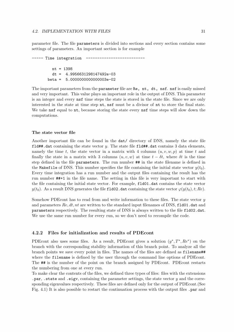
After creating the IO routines we have to test if the routines work properly. We give now thedescription of our test. The test gives an idea how the PDEcont is connected to DNS. Thefollowing situation is executed with a small C program which is just a sequence of calls to theIO routines. It is a test of the communication between a C program and the DNS code withfiles.
Imagine we start with y∗(t0) on the branch of periodic solutions and call it point1. Wehave two data files of this point1, namely point1.par with the parameter settings andpoint1.state containing the state y∗(t0) = (u∗(t0), v
∗(t0)). The routine ReadPar reads theinitial parameters from point1.par. ReadState reads the state from point1.state andWriteState copies it to fld01.dat. This file fld01.dat contains the initial vector field(u∗(t0), v
∗(t0), w = 0, p = 0) for the DNS code. Assume that after the first call of ReadPar
the parameters are changed by PDEcont. The new parameter values are copied with WritePar
to the standard parameter file parameters.Now DNS has the necessary files to integrate y∗(t0) over a time interval nt*dt at Re. Asa result we have fld02.dat with the corresponding parameter settings parameters. Thesefiles are again read and written to the resulting files point2.par and point2.state. Noticethat the format of these resulting files is in such a way that the process can be repeated.After the test it is very important that no data is missing. Furthermore we have to makesure that no digits are lost. After calling ReadPar and Writepar we compare a small part
34 CHAPTER 4. IMPLEMENTATION
ReadPar
WritePar
ReadState
WriteState
DNS
fld02.dat
WriteState
Readstate
Change parameters
ReadPar
WritePar
point1.statepoint1.par
fld01.dat
point2.par point2.state
parameters
Figure 4.2: Schematic view of the communication between DNS and the C program which usesthe IO routines.
of point1.par with parameters. Between the read and write routines there is a parameterchange. We present a part of the files below to show that ReadPar and Writepar works fine.
point1.par
----- Physical parameters ------------------------
Re = 8.0000000000000000e+01
----- Time integration --------------------------
nt = 60
dt = 2.0000000000000000e-03
beta = 8.0000000000000002e-02
parameters
4.2. IMPLEMENTATION WITH FILES 35
----- Physical parameters ------------------------
Re = 9.0000000000000000e+01
----- Time integration --------------------------
nt = 70
dt = 2.0000000000000000e-03
beta = 8.0000000000000002e-02
Furthermore we compare the first few lines of the state files fld02.dat resulting from DNSwith point2.state after calling ReadState and WriteState. The first line of both filescontains the time t at which this state occurs. Then follows the state y(t) at time t. Note thedifference expained between the .dat file and the .state file as explained.
fld02.dat
0.3002000000000010E+03
0.0000000000000000E+00 0.1000000000000000E+01 ... ...
0.6377042586634170E-05 0.1000000000000000E+01 ... ...
0.1256226285825501E-04 0.1000000000000000E+01 ... ...
0.1855667991431518E-04 0.1000000000000000E+01 ... ...
0.2438159870673748E-04 0.1000000000000000E+01 ... ...
point2.state
3.0020000000000101e+02
0.0000000000000000e+00 1.0000000000000000e+00 ... ...
6.3770425866341704e-06 1.0000000000000000e+00 ... ...
1.2562262858255010e-05 1.0000000000000000e+00 ... ...
1.8556679914315180e-05 1.0000000000000000e+00 ... ...
2.4381598706737479e-05 1.0000000000000000e+00 ... ...
The test program is executed successfully. From this test we can conclude that with the fourIO routines it is possible to let a C program, like PDEcont, and a Fortran program exchangedata with each other.
4.2.5 Implementation of the system definition
PDEcont is a continuation code, but the code doesn’t know anything about our flow problemand its governing equations. We now continue with the implementation of our flow problem.In PDEcont a system definition API is defined [22], Application Program Interface. This is aset of routines which are needed for the implementation of a system. This is possible, because

36 CHAPTER 4. IMPLEMENTATION
for a stability analysis PDEcont always needs the same ingredients. These ingredients areshown in Chapter 2. A programmer can use these routines to implement a system and letPDEcont perform a bifurcation analysis on it. The input and output of the routines arealready defined in the code [22]. The programmer has to program the routines.
System API
The following routines are used to implement a system :
• SysInit(): This is the initialization phase of the system. The routine reads settingsfrom the configuration file, not related with the calculations. For example the filenamefilename containing the initial state y and parameter settings or some time integrationsettings.
• SysHelp() : This routine gives information about the system and its parameters.
• SysStart(): Read starting state y, period T expressed in dt and nt, value of branchingparameter Re. These values are found in the file defined in the routine SysInit.
• SysPrintStateR(): Prints certain data to screen.
• SysStoreState(): This routine can be used to create the files filename##.par, filename##.stateand filename##.eigv. The files get a unique number for every new point on the branch.The filename is specified by the user with a PDEcont command line option.
• SysRHS(): In this routine the user can define the f(y, γ). We do not need this routinein our experiments.
• SysIntegrate(): This routine integrates over a time interval T . Due to the choice ofthe implementation method this routine contains the connection to DNS code by meansof the IO routines. It also returns the derivative of the state y with respect to T whenneeded.
• SysMV(): Matrix vector multiplication with a matrix like the monodromy matrix. Thismultiplication is the directional derivative of ϕ in the direction of vector v. This routinecomputes MVp in the iteration scheme of (3.16) and is also used in the Picard iterations.
• SysDDpar():This routine computes the derivative of ϕ with respect to the continuationparameter Re.
• SysSysDim(): This routines returns the dimension of our system.
For the implementation of our flow problem in PDEcont we have to program the API routines.Together with our IO routines PDEcont must be able to do a numerical bifurcation analysis.We know from Chapter 2, PDEcont solves the new point on the branch by iterating to theexact solution y∗. For this, PDEcont needs the derivatives of ϕ with respect to T and γ andmatrix-vector products with M = ∂ϕ/∂y. For this the routines SysIntegrate, SysDDpar
and SysMV are used. We explain these most important routines in detail.

4.2. IMPLEMENTATION WITH FILES 37
SysInit
This routine reads some values of variables. The values of these variables do not changeduring the calculation of a branch of solutions. All these values are stored in a configuration(Cfg) file. In our case the following values are read from the Cfg file:-fname: The name of the file containing the starting point on a branch-diff order: The order of the finite difference method for computing a derivative-h difference: Determines the finite difference stepsize.-integration info: Value for printing the used finite difference method to screen.
Also some memory for workspaces is reserved.
SysStart
This routine reads from the file, specified in the SysInit routine, the initial branching pa-rameter value Re, initial value of the period T and the initial state vector y. This routineis used only in the start of PDEcont. Here comes the IO routines in use, namely ReadPar
and ReadState. The length of the time interval T must be calculated from dt and nt. Thisroutine also creates the grid for the DNS code.
SysIntegrate
In our experiment this routine is in fact the connection to the DNS code. It looks very similarto our IO routine test. This routine sends the state y, T and Re to DNS. DNS returns theresult ϕ(y, T ;Re). In Chapter 4.2.1, we saw that in result file fld##.dat the final state andthe state at a previous time step can be found. In combination with the time step dt wemake a first order approximation of
∂ϕ(y(t0), T,Re)
∂T≈
ϕ(y(t0), T,Re) − ϕ(y(t0), T − dt,Re)
dt. (4.1)
This derivative is only computed when computing a periodic solution.
SysMV
In the iteration process (3.16) we can see that at every iteration step we need the matrix vectormultiplication MV where V contains p vectors. It is also needed in the Picard iterationprocess. The matrix-vector multiplication MV is computed by a finite difference method.For the directional derivative a first, second and fourth order finite difference method isimplemented. The user can choose the order in the configuration file. The value of h is alsodefined in the this file. The settings for the finite differences are initialized in the SysInit
routine. We used a first order approximation of the matrix vector multiplication, namely
M(y(t0), T,Re)v ≈ϕ(y(t0) + hv, T,Re) − ϕ(y(t0), T,Re)
h, (4.2)
38 CHAPTER 4. IMPLEMENTATION
in all our experiments. Here
h = hdifference||u||2||v||2
. (4.3)
SysDDpar
The derivative of ϕ with respect to the branching parameter Re is calculated with this routine.For this derivative we also use a finite difference technique. Here it is also possible to use afirst, second or fourth order method. The settings of this finite difference method are equalto the settings from SysMV, hence in all our experiments we used a first order approximationof this derivative,
∂ϕ(y(t0), T,Re)
∂Re≈
ϕ(y(t0), T,Re + h) − ϕ(y(t0), T,Re)
h. (4.4)
SysStoreState
When a branch point (y∗, T ∗, Re∗) is found, this routine creates the files .state, .par and.eigv containing the state vector y∗, parameters T,Re and the corresponding eigenvaluesrespectively. The latter file gives us the stability information. With Matlab we can visualizethe results. (See Section 4.3).
SysPrintStateR
This routine prints the following data to screen: the 2 norm of the u and v component, thecurrent value of the branching parameter Re and the current value of the period T .
All these routines together with the IO routines must be programmed is a C file called thesystem implementation file. After the proper configuration of the Makefile of PDEcont theroutines from system implementation file will be implemented in PDEcont.
4.3 Matlab
As a result of defining the special files .par, .state and .eigv we are forced to create aMatlab routine to read all the data from these specific files for visualizing the results. We areinterested in the stability of the branch points calculated in a specific range of the physicalparameter Re. Every branch point, which represents the state vector y∗ in the .state file hasa corresponding .par file which gives the location of Re and the stability information in the.eigv file. To get a good overview of the stability of the branch points y∗ in a certain rangeof Re we have to collect for every Re value from the .par files the corresponding stabilityinformation from .eigv files. Since we have two regimes in our flow problem, namely thesteady-state and the periodic regime we have two different procedures in our Matlab routine.In the steady-state regime, the routine collects at every branch point y∗i the correspondingRei number and the right most eigenvalue λi and plot this λi as function of Rei.In the periodic regime, the routine collects at every branch point y∗i the corresponding Rei

4.3. MATLAB 39
number and the largest in modulus non trivial Floquet multiplier µi and plots this µi asfunction of Rei.

40 CHAPTER 4. IMPLEMENTATION

Chapter 5
Results
In this project we have two goals, namely the numerical bifurcation analysis of the flowproblem and finding out if the Newton-Picard method in PDEcont works with the DNS codefor this problem. For the second goal of this project the discretization errors in DNS arenot very important. However, for our first goal it is nice to have results which are in goodagreement with results from literature. Therefore we did calculations on different domains.To study the combination of PDEcont and DNS we used a small domain with relatively fewcells. To find the Hopf bifurcation we used a larger domain with more cells. The flow problemis situated in a space with no boundaries. Probably our results are better when we chooseour domain very large, such that the boundary conditions have no influence on the cylinderwake.
5.1 Results with simulation
5.1.1 Estimates of the eigenvalues
First we choose a suitable observation point in the calculation domain, not far from thecylinder, where a lot is happening with the flow. This point corresponds to the ith componentof the state vector y ∈ R
n. To investigate the stability of the system, we follow the trajectoryof the yi = (ui, vi) components in this fixed point. When we are in the steady state regimeRe < 46, the trajectory of the solution yi(t) will converge to y∗i for t → ∞. In time, yi(t) willapproximately evolve as
yi(t) − y∗i ≈ eλdt(yi(t0) − y∗i ) (5.1)
where λd is the dominant eigenvalue of A. With these trajectories of ui or vi we can makeestimates of this dominant eigenvalue λd which determines the rate of convergence to y∗i .
For the periodic solution at Re > 46, we can do something similar. Any trajectory startingclose enough to the periodic solution will converge to it, and the asymptotic speed at whichthis happens is governed by the dominant non-trivial Floquet multiplier µd.
Estimate the rightmost eigenvalues of the steady state
If we follow the rightmost eigenvalues λd when Re goes to the critical Reynolds number Rec,we shall see that there is a pair of complex conjugate eigenvalues leaving the complex left
41

42 CHAPTER 5. RESULTS
half plane. At Rec ≈ 46, <(λd) = 0 and =(λd) = β 6= 0. We will now estimate the complexpart of λd from the trajectory yi(t). For this estimate we used the grid with domain sizea = 30, b = 20 and number of grid points nx = 200, ny = 240, because the results from ourexperiments using this grid are in good agreement with the results from literature.We calculated the trajectory yi(t) at Re = 45 with initial state yi(t0) at Re = 47. From thistrajectory we can estimate β close to the Hopf bifurcation. The trajectory yi(t) is shown inthe left panel of Fig. 5.1. We can make an estimate of β from the frequency f = T−1 of thevelocity component ui(t) of yi(t). From the yi(t) follows f ≈ 0.117 and thus β = 2πf ≈ 0.74.Near the Hopf bifurcation, at Re = 45, the dominant eigenvalue has =(λd) ≈ 0.74.In the left panel of Fig. 5.1, we see that the maximum of the amplitude of the oscillationsdecreases over time which means that <(λd) < 0. To estimate the rate of convergence we usethe amplitude of yi(t). We denote E[j] as the jth maximum of yi(t) − y∗i . Then from (5.1)E[j] approximately evolves as
E[j+1] ≈ e<(λd)T E[j]. (5.2)
Taking the logarithm of (5.2) we obtain
ln E[j+1] ≈ <(λd)T + ln E[j], (5.3)
and finally
<(λd) ≈ln E[j+1] − ln E[j]
T. (5.4)
From the right panel of Fig. 5.1 we can estimate the real part. As a result we estimated<(λd) ≈ −0.0082, where T = f−1 ≈ 8.547.With this result we can validate the stability analysis from PDEcont in the neighbourhoodwhen following the branch of steady states.
0 10 20 30 40 50−0.07
−0.06
−0.05
−0.04
−0.03
−0.02
−0.01
0
time
u
1 2 3 4 5 6
−4
−3.95
−3.9
−3.85
−3.8
−3.75
−3.7
−3.65
−3.6
−3.55
j
ln E
[j]
Figure 5.1: Left : Velocity ui(t) (solid curve) in a fixed point against time at Re = 45. Thedashed line is the stable steady state. Right : The ln E[j] as function j.
Estimate dominant Floquet multiplier Re > 46
To estimate this multiplier at Re = 47, close to the Hopf bifurcation point, we first determinedthe maximum of the velocity component ui at our observation point. Then we started a
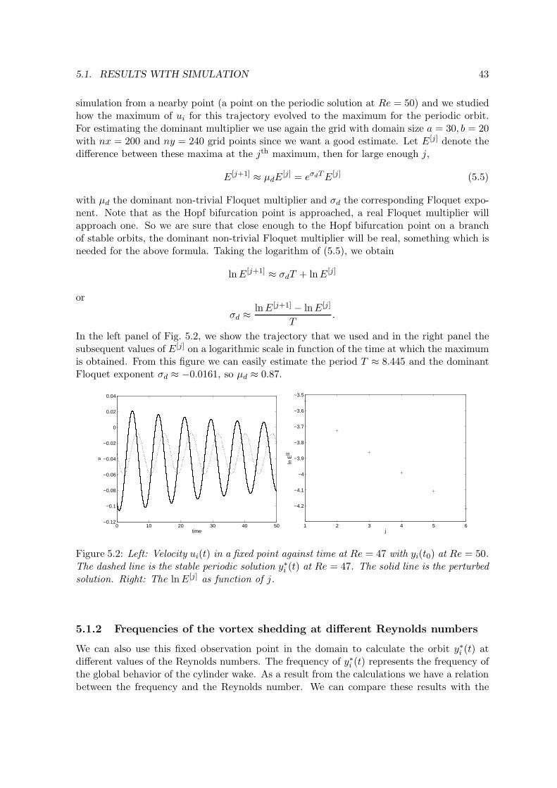
5.1. RESULTS WITH SIMULATION 43
simulation from a nearby point (a point on the periodic solution at Re = 50) and we studiedhow the maximum of ui for this trajectory evolved to the maximum for the periodic orbit.For estimating the dominant multiplier we use again the grid with domain size a = 30, b = 20with nx = 200 and ny = 240 grid points since we want a good estimate. Let E[j] denote thedifference between these maxima at the jth maximum, then for large enough j,
E[j+1] ≈ µdE[j] = eσdT E[j] (5.5)
with µd the dominant non-trivial Floquet multiplier and σd the corresponding Floquet expo-nent. Note that as the Hopf bifurcation point is approached, a real Floquet multiplier willapproach one. So we are sure that close enough to the Hopf bifurcation point on a branchof stable orbits, the dominant non-trivial Floquet multiplier will be real, something which isneeded for the above formula. Taking the logarithm of (5.5), we obtain
ln E[j+1] ≈ σdT + ln E[j]
or
σd ≈ln E[j+1] − ln E[j]
T.
In the left panel of Fig. 5.2, we show the trajectory that we used and in the right panel thesubsequent values of E[j] on a logarithmic scale in function of the time at which the maximumis obtained. From this figure we can easily estimate the period T ≈ 8.445 and the dominantFloquet exponent σd ≈ −0.0161, so µd ≈ 0.87.
0 10 20 30 40 50−0.12
−0.1
−0.08
−0.06
−0.04
−0.02
0
0.02
0.04
time
u
1 2 3 4 5 6
−4.2
−4.1
−4
−3.9
−3.8
−3.7
−3.6
−3.5
j
ln E
[j]
Figure 5.2: Left: Velocity ui(t) in a fixed point against time at Re = 47 with yi(t0) at Re = 50.The dashed line is the stable periodic solution y∗i (t) at Re = 47. The solid line is the perturbedsolution. Right: The ln E[j] as function of j.
5.1.2 Frequencies of the vortex shedding at different Reynolds numbers
We can also use this fixed observation point in the domain to calculate the orbit y∗i (t) atdifferent values of the Reynolds numbers. The frequency of y∗i (t) represents the frequency ofthe global behavior of the cylinder wake. As a result from the calculations we have a relationbetween the frequency and the Reynolds number. We can compare these results with the
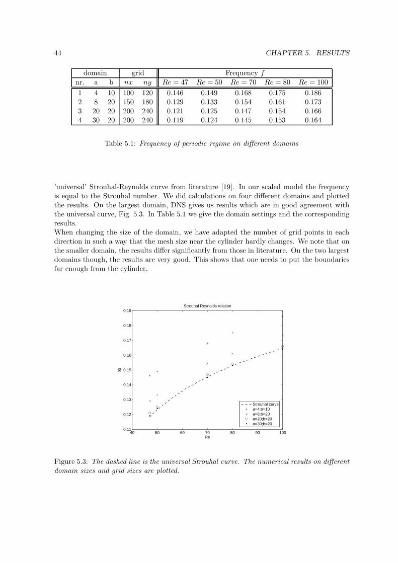
44 CHAPTER 5. RESULTS
domain grid Frequency f
nr. a b nx ny Re = 47 Re = 50 Re = 70 Re = 80 Re = 100
1 4 10 100 120 0.146 0.149 0.168 0.175 0.1862 8 20 150 180 0.129 0.133 0.154 0.161 0.1733 20 20 200 240 0.121 0.125 0.147 0.154 0.1664 30 20 200 240 0.119 0.124 0.145 0.153 0.164
Table 5.1: Frequency of periodic regime on different domains
’universal’ Strouhal-Reynolds curve from literature [19]. In our scaled model the frequencyis equal to the Strouhal number. We did calculations on four different domains and plottedthe results. On the largest domain, DNS gives us results which are in good agreement withthe universal curve, Fig. 5.3. In Table 5.1 we give the domain settings and the correspondingresults.When changing the size of the domain, we have adapted the number of grid points in eachdirection in such a way that the mesh size near the cylinder hardly changes. We note that onthe smaller domain, the results differ significantly from those in literature. On the two largestdomains though, the results are very good. This shows that one needs to put the boundariesfar enough from the cylinder.
40 50 60 70 80 90 1000.11
0.12
0.13
0.14
0.15
0.16
0.17
0.18
0.19
Re
St
Strouhal Reynolds relation
Strouhal curvea=4;b=10a=8;b=20a=20;b=20a=30;b=20
Figure 5.3: The dashed line is the universal Strouhal curve. The numerical results on differentdomain sizes and grid sizes are plotted.
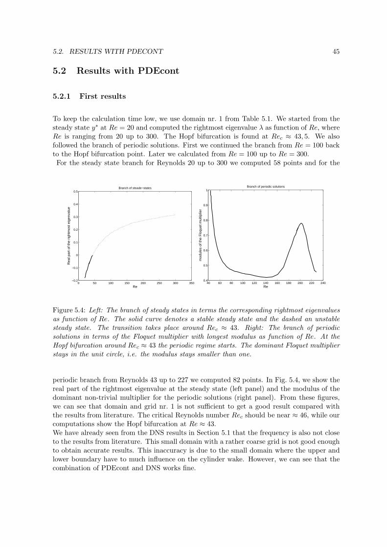
5.2. RESULTS WITH PDECONT 45
5.2 Results with PDEcont
5.2.1 First results
To keep the calculation time low, we use domain nr. 1 from Table 5.1. We started from thesteady state y∗ at Re = 20 and computed the rightmost eigenvalue λ as function of Re, whereRe is ranging from 20 up to 300. The Hopf bifurcation is found at Rec ≈ 43, 5. We alsofollowed the branch of periodic solutions. First we continued the branch from Re = 100 backto the Hopf bifurcation point. Later we calculated from Re = 100 up to Re = 300.For the steady state branch for Reynolds 20 up to 300 we computed 58 points and for the
0 50 100 150 200 250 300 350−0.2
−0.1
0
0.1
0.2
0.3
0.4
0.5
Re
Rea
l par
t of t
he r
ight
mos
t eig
enva
lue
Branch of steade−states
40 60 80 100 120 140 160 180 200 220 2400.4
0.5
0.6
0.7
0.8
0.9
1
Re
mod
ules
of t
he F
loqu
et m
ultip
lier
Branch of periodic solutions
Figure 5.4: Left: The branch of steady states in terms the corresponding rightmost eigenvaluesas function of Re. The solid curve denotes a stable steady state and the dashed an unstablesteady state. The transition takes place around Rec ≈ 43. Right: The branch of periodicsolutions in terms of the Floquet multiplier with longest modulus as function of Re. At theHopf bifurcation around Rec ≈ 43 the periodic regime starts. The dominant Floquet multiplierstays in the unit circle, i.e. the modulus stays smaller than one.
periodic branch from Reynolds 43 up to 227 we computed 82 points. In Fig. 5.4, we show thereal part of the rightmost eigenvalue at the steady state (left panel) and the modulus of thedominant non-trivial multiplier for the periodic solutions (right panel). From these figures,we can see that domain and grid nr. 1 is not sufficient to get a good result compared withthe results from literature. The critical Reynolds number Rec should be near ≈ 46, while ourcomputations show the Hopf bifurcation at Re ≈ 43.We have already seen from the DNS results in Section 5.1 that the frequency is also not closeto the results from literature. This small domain with a rather coarse grid is not good enoughto obtain accurate results. This inaccuracy is due to the small domain where the upper andlower boundary have to much influence on the cylinder wake. However, we can see that thecombination of PDEcont and DNS works fine.

46 CHAPTER 5. RESULTS
domain grid Hopf bifurcation Rc
nr. a b nx ny Rec
1 4 10 100 120 43.75 < Rec < 43.852 8 20 150 180 45.46 < Rec < 45.563 20 20 200 240 45.96 < Rec < 46.064 30 20 200 240 46.34 < Rec < 46.43
Table 5.2: The location of Hopf on different domains
5.2.2 The Hopf bifurcation
We can locate the Hopf bifurcation at Rec by starting the continuation process on both sidesof the bifurcation point Re ≈ 46. We start on the steady state branch and continue thebranch until the real part of the dominant eigenvalue becomes positive. The point where<(λ) = 0 marks the Hopf bifurcation.We can also start the continuation process on the periodic branch and follow the branch untilthe non-trivial dominant Floquet multiplier becomes one, i.e., there are two Floquet multi-pliers equal to one which marks the beginning of the periodic regime. This should be closeto the the initial Reynolds number found during the continuation of the steady state branch.In the previous section we showed that on a small domain with a coarse grid, the results arenot accurate enough.
Starting in steady state regime
Now we present the results of more accurate computations for locating the Hopf bifurcationRec. These computations are performed on different domains and grids, also used in Section5.1. In Table 5.2 we present the boundaries of the interval in which the Hopf bifurcation canbe found. Fig. 5.5 shows the real part of the rightmost eigenvalue pair for the four grids. Thelocation of the Hopf bifurcation Rec is marked where these curves crosses the value zero.
We can see from Fig. 5.5 that the location of the Hopf bifurcation Rec gets closer to the valuefrom literature Rec ≈ 46 [3] when our domain gets larger. The walls at x = ±a have muchinfluence on the behavior of the cylinder wake. For good results these must be far away fromthe cylinder, i.e., a should be very large.
In Section 5.1 we estimated the complex part of the dominant eigenvalue λd at Re = 45,near the Hopf bifurcation. The estimate is done from computations on the largest domainwith the most accurate grid we used. With this estimate we can validate the results fromPDEcont. At Re ≈ 45 the imaginary part of the rightmost eigenvalue computed by PDEcontis approximately 0.73 which is close to our estimate from the simulation. It is not reallypossible to compare the real parts of the rightmost eigenvalue from PDEcont and the esti-mate, because these values are too small. But since the imaginary part is already close to ourestimate, the combination of PDEcont and DNS gives good results for the steady state regime.

5.2. RESULTS WITH PDECONT 47
43 43.5 44 44.5 45 45.5 46 46.5 47−16
−14
−12
−10
−8
−6
−4
−2
0
2x 10
−3
Re
Rea
l par
t of t
he r
ight
mos
t eig
enva
lue
Hopf bifurcation
a=4;b=10a=8;b=20a=20;b=20a=30;b=20
Figure 5.5: Curves of the real part of the rightmost eigenvalues as function of the Reynoldsnumber on different domains and grid sizes.
Starting in the periodic regime
In Fig. 5.6 the results of the dominant Floquet multiplier µd as function of Reynolds atdifferent domain sizes and grids are presented. We can see that from the other side of thebifurcation point, the Rec marks the beginning of the periodic branch and the dominant non-trivial Floquet multiplier is 1.
We also estimated the dominant Floquet multiplier µd close to the Hopf bifurcation in Section5.1. The non trivial dominant Floquet multiplier computed by PDEcont is approximately 0.96which does not at all match with our estimate 0.88 from simulation. The estimated periodT ≈ 8.445 is close to the period computed by PDEcont T = 8.463. It is not clear what causesthe discrepancy between the estimate of the Floquet multiplier and the computed value.

48 CHAPTER 5. RESULTS
43.5 44 44.5 45 45.5 46 46.5 470.82
0.84
0.86
0.88
0.9
0.92
0.94
0.96
0.98
1
Re
mod
ules
of t
he F
loqu
et m
ultip
lier
Hopf bifurcation
a=4;b=10a=8;b=20a=20;b=20a=30;b=20
Figure 5.6: A plot of the dominant Floquet multiplier µ as function of Re. The periodicregime starts where the dominant Floquet multiplier becomes equal to one.
5.3 Performance
Clustering of the Floquet multipliers
In the Newton-Picard method of PDEcont, we have to choose a radius ρ which defines whichFloquet multiplier are considered to be “large” and are included in the dominant subspace. Ifthe number of such vectors is too large, the Newton-Picard method becomes inefficient. Theoptimal value of ρ is problem dependent. In our flow problem, we varied the ρ at differentparts on the branches, since we sometimes had convergence problems. In our flow problemmost Floquet multipliers are clustered around zero. This is a good condition for PDEcont.In Fig. 5.7 we see the dominant Floquet multipliers. Since we used ρ ≈ 0.5, we typically hadonly about 2 basis vectors.
Computation time
To give an idea of the computation times, we approximated the time needed to compute asteady state or a periodic branch point with different domains. The choice of radius ρ in theNewton-Picard process has a lot of influence on the computation times. These are shown inTables 5.3 and 5.4. Computing the full branch of steady state solutions on grid nr. 1 (58points) took about 3.5 days, computing the whole branch of periodic solutions (82 points)about 5 days. So the computations are very time-consuming. A speedup should come from aparallel implementation of the CFD code.
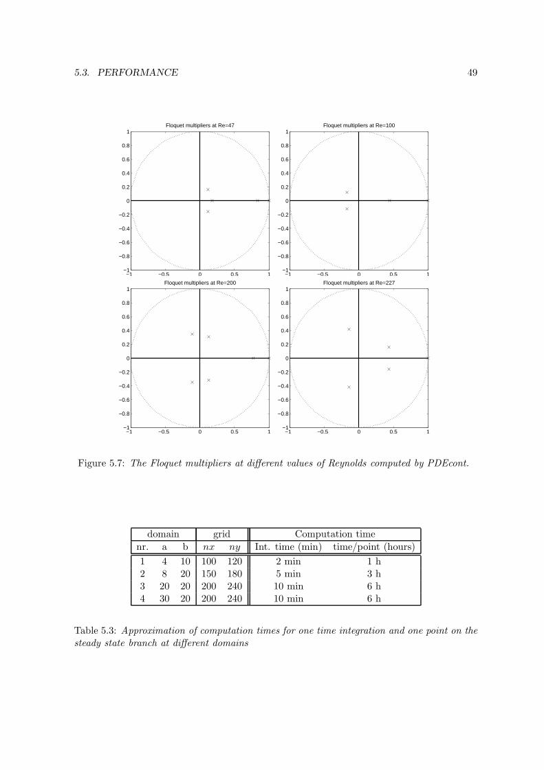
5.3. PERFORMANCE 49
−1 −0.5 0 0.5 1−1
−0.8
−0.6
−0.4
−0.2
0
0.2
0.4
0.6
0.8
1Floquet multipliers at Re=47
−1 −0.5 0 0.5 1−1
−0.8
−0.6
−0.4
−0.2
0
0.2
0.4
0.6
0.8
1Floquet multipliers at Re=100
−1 −0.5 0 0.5 1−1
−0.8
−0.6
−0.4
−0.2
0
0.2
0.4
0.6
0.8
1Floquet multipliers at Re=200
−1 −0.5 0 0.5 1−1
−0.8
−0.6
−0.4
−0.2
0
0.2
0.4
0.6
0.8
1Floquet multipliers at Re=227
Figure 5.7: The Floquet multipliers at different values of Reynolds computed by PDEcont.
domain grid Computation time
nr. a b nx ny Int. time (min) time/point (hours)
1 4 10 100 120 2 min 1 h2 8 20 150 180 5 min 3 h3 20 20 200 240 10 min 6 h4 30 20 200 240 10 min 6 h
Table 5.3: Approximation of computation times for one time integration and one point on thesteady state branch at different domains

50 CHAPTER 5. RESULTS
domain grid Computation time
nr. a b nx ny Int. time (min) time/point (hours)
1 4 10 100 120 1.5 min 1.5 h2 8 20 150 180 4.5 min 4.5 h3 20 20 200 240 8.5 min 8.5 h4 30 20 200 240 8.5 min 9.5 h
Table 5.4: Approximation of computation times for one time integration and one point on thebranch of periodic solutions at different domains
Chapter 6
Evaluation
In this project we had two objectives, namely the numerical bifurcation analysis of our flowproblem and finding out if PDEcont does work for our flow problem and with this DNS code.We showed in Chapter 5 that with the combination of PDEcont and DNS it is possible tocompute the steady state and periodic branch in a whole range of Reynolds numbers. Wewill see that there is an interesting event on the branch of periodic solutions which can leadto further research.We also showed that it is possible to locate the Hopf bifurcation very accurately. The locationof the Hopf bifurcation is in good agreement with the result from literature.
6.1 Implementation difficulties and possible weaknesses in the
combination
We are very satisfied with the results obtained with the combination of PDEcont and theDNS code. There were no real problems in the implementation of DNS in PDEcont with themethod used. However, due to the implementation method we used, it was hard to find errorswhen something went wrong. The DNS code and PDEcont only communicate with each otherby files. In this way it is hard to find possible errors when a time integration fails in the DNScode, because PDEcont has not enough control over the time integration. Probably with thesecond implementation method, mentioned in Chapter 4, it would have been easier to findsuch rare errors. This is an inconvenience in the combination of PDEcont and DNS, but it isa consequence of the chosen implementation method.We mention also three small things which need some extra attention. First we have tonotice that since PDEcont uses the output of DNS for further calculations, this output mustbe accurate enough. We changed the number of digits of the output of DNS to obtain thenecessary accuracy for PDEcont. A second issue we encountered was the fact that for startingthe DNS code, we also needed the state at the previous time step. The previous state was notcomputed by PDEcont and thus we copied the current state instead of the previous state. Asa result the time integration method will behave like a forward Euler method instead of anAdams-Bashforth method in the first time step. Thirdly, in the current implementation, thesimulation code runs in its source directory and all the paths are hard-coded in the systemdefinition files. We need to switch to a more flexible setup to make it possible to run severalinstances of the code on a single machine, each in its own directory, without having to changethe source for each test.
51
52 CHAPTER 6. EVALUATION
We can conclude that the combination works perfectly, but an other implementation methodwould probably be more proper.
6.2 Performance
This flow problem is very suitable for PDEcont since the spectrum of the Floquet multipliersis nicely clustered (see Fig. 5.7). For accurate results with the combination of PDEcont andDNS, we need domain nr. 4 in our experiments. This results in very long computation timesas we saw in Table 5.3 and 5.4. For this reason we did not compute the steady state andperiodic branch in the range of Reynolds 20 up to 300 on this grid.We did compute these branches in this range on domain nr. 1 to show that we are able tocompute branches in a whole range of Reynolds numbers. We computed the branch of steadystates very successfully. The branch of periodic solutions has some convergence problemsat Re ≈ 227. At this branch point the Floquet multipliers are still nicely clustered. Theproblems already occur in the computation of the basis. It is very likely that the finitedifference used for the matrix-vector products are not longer accurate enough and we suspectthat this is caused by non-smooth behaviour of the DNS code. It is possible that the DNScode is not sufficiently ’smooth’. To continue the branch from Re ≈ 227 we could try thefollowing:-Increase the accuracy of the Poisson solver in the DNS code,-Fix the number of iteration steps in the Poisson solver,-Use a higher order finite difference method in PDEcont to compute the derivatives of ϕ.However, if the failure is caused by too non-smooth behaviour of the DNS code, this will beof little help.For computing the matrix-vector products and the derivatives of ϕ with respect to T and Re,a first order finite difference method was sufficient for our flow problem for smaller Reynoldsnumbers.
6.3 Further research
Notice that in the periodic regime the Floquet multiplier with largest modulus is increasingvery fast around Re ≈ 170. After a local maximum at Re ≈ 200 the Floquet multiplierdecreases in modulus and does not leave the unit circle (see right Fig. 5.4). This event mighthave something to do with the second instability around Re ≈ 189.We used the DNS code in a two dimensional mode to find the steady state and the peri-odic branch. Unfortunately, due to the two dimensional mode of DNS, we were not ableto find the second instability at Re ≈ 189. There is a possibility to use the DNS code in athree dimensional mode and try to find the second instability as Barkley did in his research [4].

Appendix A
Description of subroutines for data
transfer
ReadPar
Synopsis
int ReadPar(par fname in, sdir)
Description of Parameters
char *par fname in: Read the parameters from this file.char *sdir: The directory of the source file.
Return values
IO SUCCESS, 0 : SuccessfulIO FAILURE, 1 : Failed
Action
The routine ReadPar() reads the parameter settings from the DNS code such that PDEcontcan use the necessary parameter values. The following parameters and their values can befound in the input file:branching parameter, the Reynolds number : Re,time step : dt,number of time steps : nt,time integration parameter : nsf.
WritePar
Synopsis
int WritePar(par fname in, par fname out, sdir, ddir )
Description of Parameters
char *par fname in: File name to copy the unchanged parameters from.char *par fname out: The file name with the new parameters.char *sdir: The directory of the source file.
53

54 APPENDIX A. DESCRIPTION OF SUBROUTINES FOR DATA TRANSFER
char *ddir: The destination directory of the new file.
Return values
IO SUCCESS, 0 : SuccessfulIO FAILURE, 1 : Failed
Action
The routine WritePar() writes the new parameter values to a given file name in the destina-tion directory. This new can be read by the DNS code. This routine reads the parametersfrom the input file. The unchanged parameter values are copied from the input file to thenew file. The following parameter values can be updated in a new file:branching parameter, Reynolds number : Re,time step : dt,number of time steps : nt,time integration parameter : nsf.
ReadState
Synopsis
int ReadState(state fname in, state, state o, sdir)
Description of Parameters
char *state fname in : File to read the state vector from.double *state: Pointer to state vector.double *state o: Pointer to old state, one time step before state.char *sdir: The directory of the sourse file.
Return values
IO SUCCESS, 0 : SuccessfulIO FAILURE, 1 : Failed
Action
The routine ReadState() reads the state (u, v,w, p) from fldxx.dat. It converts the vectors uand v into one vector (u(1), v(1), u(2), v(2), · · · , u(total), v(total)), where total is the totalnumber of grid points. The column vector is stored in the variable state. The w and pcomponents in the fld##.dat file are not stored in memory.The previous time step is storedin the variable state o. The routine has to know the total number of discritization points.The total length of a column vector in the standard DNS state input file fld##.dat is 3 timestotal. It contains 3 identical 2D vector fields (u, v,w, p). Of course only one is read.
WriteState
Synopsis
int WriteState(state fname out, state, state o, ddir)

55
Description of Parameters
char *state fname out : Write the state vector to this file.double *state: Pointer to state vector.double *state o: Pointer to old state, one time step before state.char *ddir: The destination directory of the file.
Return values
IO SUCCESS, 0 : SuccessfulIO FAILURE, 1 : Failed
Action
The routine WriteState() writes the known state in memory [u(1), v(1), u(2), v(2), · · · ] to anew file. The format will be the standard DNS input format or to an output file of PDEcont.The two columns w and p are added as the third and fourth column in the new file. The wand p components are fixed to zero. In the case for writing a DNS input file, the current statewill be written two times to the file, since there is no old state.

56 APPENDIX A. DESCRIPTION OF SUBROUTINES FOR DATA TRANSFER

Bibliography
[1] K. Lust. Numerical bifurcation analysis of periodic solutions of partial differential equa-tions. PhD thesis, Katholieke Universiteit Leuven, 1997.
[2] R. W. C. P. Verstappen and A. E. P. Veldman. Symmetry-preserving discretization ofturbulent flow. Journal of Computational Physics, 187:343–368, 2003.
[3] C. P. Jackson. A finite-element study of the onset of vortex shedding in flow past variouslyshapes bodies. J. Fluid Mech., 182:23–45, 1987.
[4] D. Barkley. Confined three-dimensional stability analysis of the cylinder wake. PhysicalReview, E 71:1–3, 2005.
[5] E. J. Doedel, A. R. Champneys, T. J. Fairgrieve, Y. A. Kuznetsov, B. Sandstede, andX. J. Wang. AUTO97: Continuation and bifurcation software for ordinary differentialequations., 1997. Technical report.
[6] A. I Khibnik, Yu. A Kuznetsov, V. V. Levitin, and E. N. Nikolaev. Locbif, version 2:Interactive local bifurcation analyzer. CAN Expertise Centre, 1992. Amsterdam.
[7] Yu. A. Kuznetsov and V. V. Levitin. CONTENT, a multiplatform continuation environ-ment., 1996. Technical report.
[8] R. E. Bank. PLTMG, a software package for solving elliptic partial differential equations:users guide 7.0. Frontiers in Applied Mathematics. SIAM, 15 edition, 1994.
[9] D. Barkley and R.D. Henderson. Three-dimensional floquet stability analysis of thewake of a circular cylinder. J. Fluid Mech., 322:215–241, 1996.
[10] R. D. Henderson and G. E. Karniadakis. Unstructured spectral element methods forsimulation of turbulent flows. J. Comp. Phys., 122:191–217, 1995.
[11] M. F. Schatz, D. Barkley, and H. L. Swinney. Instability in spatially periodic open flow.Physics of Fluids, 7:344–358, 1996.
[12] R. D. Henderson and D. Barkley. Secondary instability in the wake of a circular cylinder.Physics of Fluids, 8:1683–1685, 1996.
[13] O. Posdziech and R. Grundmann. Numerical simulation of the flow around an infinitelong circular cylinder in the transition regime. Springer-Verslag, 2001.
[14] H. Zhang, U. Fey, and B. R. Noack. On the transition of the cylinder wake. Physics ofFluids, 7:779–794, 1995.
57
58 BIBLIOGRAPHY
[15] B. R. Noack, M. Konig, and H. Eckelmann. Three-dimensional stability analysis of theperiodic flow around a circular cylinder. Physics of Fluids, A5:1279–1281, 1993.
[16] R. Seydel. Practical Bifurcation and Stability Analyses, From Equilibrium to Chaos.Springer-Verlag, 1994.
[17] M. Provensal, C. Mathis, and L. Boyer. Benard-von Karman instability: transient andforced regimes. J. Fluid Mech., 182:1–22, 1987.
[18] M. Hammache and M. Gharib. An experimental study of the parallel and oblique vortexshedding from circular cylinders. J. Fluid Mech., 232:567–590, 1991.
[19] C. H. K. Williamson. Defining a universal and continuous Strouhal-Reynolds numberrelationship for the laminar vortex shedding of a circular cylinder. Physics of Fluids,31:2742–2744, October 1988.
[20] C. H. K Williamson. Oblique and parallel modes of vortex shedding in the wake of acircular cylinder at low reynolds numbers. J. Fluid Mech., 206:579–627, 1989.
[21] F. W. Wubs. Computational methods of science. Rijksuniversiteit Groningen, 2003.
[22] K. Lust. PDEcont, a timestepper-based continuation code for large-scale systems., 1997.Technical report.