a novel trigonometric localization system for experimental ... · a novel localization system for...
TRANSCRIPT
A NOVEL LOCALIZATION SYSTEM FOR EXPERIMENTAL
AUTONOMOUS UNDERWATER VEHICLES
by
Russell Walter Morin
_________________________
A Thesis
Submitted to the Faculty
of the
WORCESTER POLYTECHNIC INSTITUTE
in partial fulfillment of the requirements for the
Degree of Master of Science
In
Mechanical Engineering
April 16, 2010
APPROVED:
Dr. Islam I. Hussein, Major Advisor
Dr. William R. Michalson, Committee Member
Dr. Alexander M. Wyglinski, Committee Member
Dr. James D. Van de Ven, Graduate Committee Representative
i
Abstract Localization is a classic and complex problem in the field of mobile robotics. It becomes
particularly challenging in an aqueous environment because currents within the water can move
the robot. A novel localization module and corresponding localization algorithm for
experimental autonomous underwater vehicles is presented. Unlike other available positioning
systems which require fixed hardware beacons, this custom built module relies only on
information available from sensors on-board the vehicle and knowledge of its bounded domain.
This allows the user to save valuable time which would otherwise be devoted to the setup and
calibration of a beacon or sensor network. The module uses three orthogonal ultrasonic
transducers to measure distances to the tank boundaries. Using the measured tri-axial orientation
of the vehicle, the algorithm analytically determines the robot’s position within the domain in
absolute coordinates. Certain vehicle states do not allow the position to be completely resolved
by the algorithm alone. In this case, state estimation is used to estimate the robot position until its
state is no longer indeterminate. The modular design of this system makes it ideal for application
on underwater vehicles which operate in a bounded environment for research purposes. An
experimental version of the module was constructed and tested in the WPI swimming pool and
showed successful localization under normal conditions.
ii
Acknowledgements I would like to extend my thanks to Professors Hussein and Michalson for the wonderful
opportunity and numerous intellectual challenges they provided to me with this thesis. This
project has cemented my view that Mechanical Engineering is an all encompassing discipline
which requires knowledge from other areas of study. I thoroughly enjoyed gaining from my
experiences while implementing theory and practice in a true WPI fashion.
I further wish to thank all those members of the WPI community who have helped me
along the way. There are too many to list, but most notable among them are Pam St. Louis,
Barbara Furhman, Barbara Edilberti, Tracey Coetzee, Tom Angelotti, Pat Morrison, and Paul
Bennett.
Finally, I would like to thank my family and friends for their love and support during this
project. They offered encouragement and listened to me when I needed motivation the most.

iii
Table of Contents Abstract i
Acknowledgements ii
Table of Contents iii
Table of Figures vi
List of Nomenclature viii
1 Introduction - 1 -
2 Localization Systems and Methods - 5 -
2.1 Passive Localization Systems - 5 -
2.2 Active Localization - 9 -
2.3 Need for a Custom Localization System - 14 -
3 Electrical Design - 15 -
3.1 Sonar Module Requirements - 16 -
3.2 Previous Work - 16 -
3.3 Sonar Signal Processing Circuit - 19 -
3.4 Receive Circuit - 20 -
3.5 Transmit Circuit - 22 -
3.6 Auxiliary Temperature Sensor - 26 -
3.7 Computer Circuit Design and Fabrication - 27 -
3.8 Sonar Module Costs - 29 -
4 Electrical Debugging and Testing - 30 -
4.1 Initial Inspection - 30 -
4.2 MSP430 Processor Testing - 30 -
4.3 Receive Circuit Testing - 31 -
4.4 Transformer Testing - 31 -
iv
4.5 Transmit Circuit Testing - 32 -
4.6 I2C Communication Testing - 38 -
4.7 Signal Attenuation Testing - 39 -
4.8 Combined Transmit and Receive Testing - 42 -
4.9 Sonar Module Diagnostics - 43 -
5 Received Signal Processing - 44 -
5.1 Hardware Signal Processing - 44 -
5.2 Software Signal Processing - 49 -
5.3 Overall Signal Processing Algorithm - 61 -
6 Trigonometric Submarine Localization - 63 -
6.1 Orientation 1 - 65 -
6.2 Determining the Tank Depth Profile - 68 -
6.3 Singular Cases - 69 -
6.4 Simulation of Submarine Localization - 71 -
7 Module Housing Design - 73 -
8 Experimental Localization Testing - 77 -
8.1 Measurements around Water Jets - 78 -
8.2 Localization Testing - 80 -
9 Conclusions - 84 -
10 Recommendations and Future Work - 85 -
11 Bibliography - 87 -
12 Appendices - 92 -
12.1 Appendix A – Electrical Schematics - 92 -
12.2 Appendix B – Board Layouts - 101 -
12.3 Appendix C - Sonar Module Cost Breakdown - 104 -
v
12.4 Appendix D – Sonar Module Diagnostics - 105 -
12.5 Appendix E – Component Datasheets - 112 -
12.6 Appendix F – Attenuation Experiment - 113 -
12.7 Appendix G – Threshold Determination Experiments - 120 -
12.8 Appendix H – Localization Algorithm Mathematics - 126 -
12.9 Appendix I – Software Explanations - 132 -
12.10 Appendix J – Attached Files - 134 -
vi
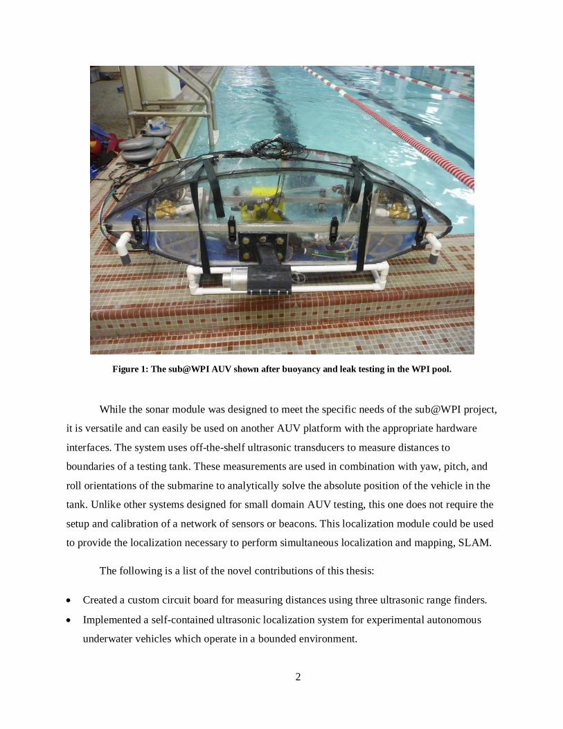
Table of Figures Figure 1: The sub@WPI AUV shown after buoyancy and leak testing in the WPI pool. - 2 -
Figure 2: A block diagram of the sonar module layout. - 15 -
Figure 3: Airmar P23 ultrasonic transducers purchased for the sonar module. - 18 -
Figure 4: Electrical schematic of the I2C circuit. - 20 -
Figure 5: Schematic of the voltage divider used to create the 1.25V reference for op-amps. - 21 -
Figure 6: The schematic layout of the PSim simulation for the custom transducer. - 25 -
Figure 7: Simulated current and voltage at the transducer from PSIM. - 26 -
Figure 8: Electrical schematic of the auxiliary temperature sensor circuit. - 26 -
Figure 9: Completed circuit board layout for the sonar module. Traces on top are red and traces
on bottom are blue. - 28 -
Figure 10: The custom circuit board for the sonar module. - 28 -
Figure 11: One of the custom wound transformers used on the sonar module. - 32 -
Figure 12: Image showing the rewiring necessary to make the transmit circuit function. - 33 -
Figure 13: Two oscilloscope traces showing the signals driving the Power MOSFETs operating
at 200 kHz. - 34 -
Figure 14: Top side of the transmit circuit test board shown with channel 1 configured. - 35 -
Figure 15: Bottom side of the transmit circuit test board shown with channel 1 configured. - 36 -
Figure 16: Two transducers placed in the water tank to test the transmit circuit. - 37 -
Figure 17: Two oscilloscope traces showing the transmitted and received signals during an early
test. - 37 -
Figure 18: Two transducers oriented towards the same wall to measure the reflected signal. - 38 -
Figure 19: Plot of the attenuation of the received ultrasonic signal over a range of distances. - 41 -
Figure 20: An example of a received pulse from initial transmitting and receiving testing. - 43 -
Figure 21: Magnitude response of the digital low-pass filter. - 52 -
Figure 22: A comparison of the filtered noise to an unfiltered noise signal in the WPI pool. - 54 -
Figure 23: The distribution of the amplitude of the filtered noise in the WPI pool. - 56 -
Figure 24: Example of the distance measurement distribution for a threshold of 1800. - 58 -
Figure 25: A graphical depiction of the signal processing algorithm to calculate the time-of-flight
of the ultrasonic signal. - 62 -
Figure 26: Depiction of the coordinate and quadrant systems for the pool. - 64 -
vii
Figure 27: The four potential situations the submarine can be in for any given angle in
orientation 1. - 65 -
Figure 28: The first potential configuration for this orientation. The sensor beams intersect with
the right and top sides of the pool as viewed from above. The corresponding equations are shown
below this caption. - 66 -
Figure 29: The second potential configuration for this orientation. The sensor beams intersect
with the left and top sides of the pool as viewed from above. The corresponding equations are
shown below this caption. - 67 -
Figure 30: The depth profile of the WPI swimming pool measured with the sonar module. - 69 -
Figure 31: The first singular case for this orientation. Only the y coordinate can be determined in
this case. - 70 -
Figure 32: The second singular case for this orientation. Only the x coordinate can be determined
in this case. - 70 -
Figure 33: Screenshot of the localization simulation program shown with the red line indicating
the submarine heading. - 72 -
Figure 34: A ProEngineer CAD assembly of the module housing and the sensors. - 73 -
Figure 35: Rapid prototyped module housing after soaking in sodium hydroxide to remove the
internal supports. - 74 -
Figure 36: Completely assembled sensor housing for the sonar module. - 75 -
Figure 37: An image from ProEngineer showing the placement and orientation of the final sonar
module on the underside of the submarine. - 76 -
Figure 38: Top side of the completed sonar module board. - 77 -
Figure 39: Bottom side of the completed sonar module board. - 78 -
Figure 40: The sensor module placed in the stream of a water jet. - 79 -
Figure 41: The sonar module placed underwater for initial localization testing. - 80 -
Figure 42: The fixture used to keep the sensor in a given location for testing. - 81 -
Figure 43: A depiction of the localization test results. - 83 -

viii
List of Nomenclature AC – Alternating current
ADC – Analog to digital convertor
ADC12 – The 12 bit analog to digital convertor in the MSP430
AUV – Autonomous underwater vehicle
CAD – Computer aided design
CAN MUVE – Coordination and Navigation of Multiple Vehicles
DC – Direct current
DFT – Discrete Fourier Transform
DMM – Digital multi-meter
DRC – Design rule checking
FIR – Finite impulse response; a type of digital filter
Gerber Files – Files generated by an electrical CAD software package which are used to manufacture a circuit board
IC – Integrated circuit
I2C – Inter-integrated circuit; a bidirectional two wire communication protocol to send data between integrated circuits
IAR – Short for IAR Embedded Workbench, the software used to interface with the MSP430
IIR – Infinite impulse response; a type of digital filter
LBL – Long baseline; a type of underwater localization system
MAC – Multiply and accumulate; a hardware accelerated multiplier on the MSP430
MATLAB – Short for Matrix Laboratory; a software package used for solving problems involving matrices
MOSFET – Metal Oxide Semiconductor Field Effect Transistor
MQP – Major Qualifying Project; an undergraduate senior-level comprehensive design experience required for graduation at Worcester Polytechnic Institute
MSP430, MSP430F2410 – A low power microprocessor from Texas Instruments used for the sonar module
Multisim – A program used to simulate electronic circuits

ix
PADS – A suite of software programs used in the design, layout and fabrication of circuit boards
PC/104 – The central processing computer onboard the sub@WPI submarine
PowerSIM – Also known as PSIM; a program used to simulate electronic circuits geared towards power electronics
ProEngineer – A mechanical CAD package used for the module housing design
Python – A free cross-platform high-level programming language
Rapid prototyping – Any method of quickly generating a model which is faster than conventional manufacturing
RealTerm – A free serial communication and capturing program
RF – Radio frequency
SLAM – Simultaneous localization and mapping
SNR – Signal to noise ratio
sub@WPI – An experimental AUV under development at Worcester Polytechnic Institute
TDOA – Time delay of arrival
TOF – Time-of-flight; the time a signal takes to travel to an object and return to the transmitting sensor.
Turns-ratio – The ratio of the number of windings on the secondary side of a transformer to the number of windings on the primary side.
USBL – Ultra-short baseline; a type of underwater localization system
WPI – Worcester Polytechnic Institute
1
1 Introduction Underwater robotics is a dynamic and rapidly expanding field of research. As the field
grows and reaches new depths, vehicles are being developed to perform increasingly complex
maneuvers with less intervention from human operators. For these experimental vehicles to
succeed in their assigned tasks they invariably require knowledge of their current position within
their environment. Without frequently updated position information, the robot can quickly drift
away from its desired location. Though many underwater positioning systems have been
developed, they are often cost prohibitive, require additional hardware external to the robot to be
placed in the environment, or are developed for use in open water. The localization systems
available, detailed in Chapter 2, would not be ideal for use in a small scale test tank, such as a
swimming pool. Because underwater vehicles must first be proven in a test environment before
moving to open water and placement of localization beacons can be a tedious process, there
exists a unique niche for a positioning system designed to localize a craft within a test tank using
only self contained hardware. The research described in this thesis seeks to fill that void by
developing a simple, versatile, and low-cost localization system suitable for research vessels
used for testing and development.
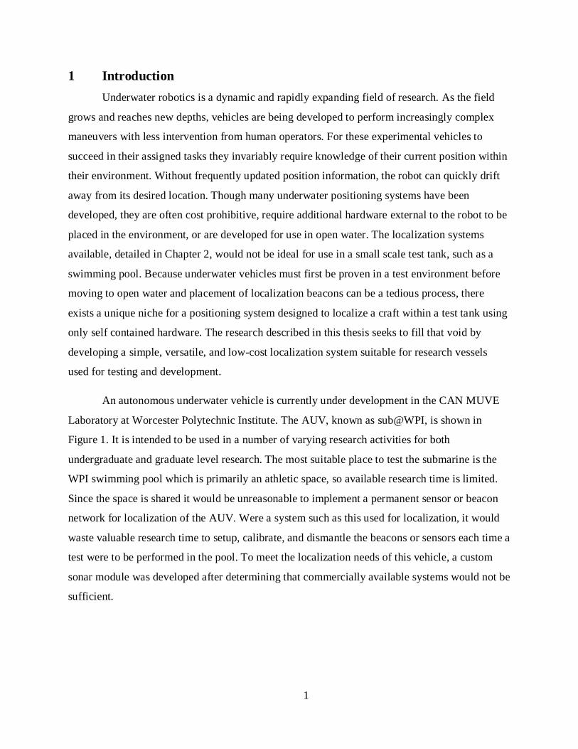
An autonomous underwater vehicle is currently under development in the CAN MUVE
Laboratory at Worcester Polytechnic Institute. The AUV, known as sub@WPI, is shown in
Figure 1. It is intended to be used in a number of varying research activities for both
undergraduate and graduate level research. The most suitable place to test the submarine is the
WPI swimming pool which is primarily an athletic space, so available research time is limited.
Since the space is shared it would be unreasonable to implement a permanent sensor or beacon
network for localization of the AUV. Were a system such as this used for localization, it would
waste valuable research time to setup, calibrate, and dismantle the beacons or sensors each time a
test were to be performed in the pool. To meet the localization needs of this vehicle, a custom
sonar module was developed after determining that commercially available systems would not be
sufficient.
2
Figure 1: The sub@WPI AUV shown after buoyancy and leak testing in the WPI pool.
While the sonar module was designed to meet the specific needs of the sub@WPI project,
it is versatile and can easily be used on another AUV platform with the appropriate hardware
interfaces. The system uses off-the-shelf ultrasonic transducers to measure distances to
boundaries of a testing tank. These measurements are used in combination with yaw, pitch, and
roll orientations of the submarine to analytically solve the absolute position of the vehicle in the
tank. Unlike other systems designed for small domain AUV testing, this one does not require the
setup and calibration of a network of sensors or beacons. This localization module could be used
to provide the localization necessary to perform simultaneous localization and mapping, SLAM.
The following is a list of the novel contributions of this thesis:
• Created a custom circuit board for measuring distances using three ultrasonic range finders.
• Implemented a self-contained ultrasonic localization system for experimental autonomous
underwater vehicles which operate in a bounded environment.
3
• Developed and validated a localization algorithm which uses three distance measurements to
the boundaries of a bounded environment to determine the absolute position of a vehicle.
Currently, there are no other systems which are designed to meet the needs of the
sub@WPI. The closest thing to the system developed in this thesis would be a localization
system using three Tritech Digital Altimeters. These modules provide distance measurements
over a range of up to 100 m with a resolution of 1 mm. They are designed for use in open water
applications, but could be adapted for the submarine. The range and resolution of these devices
come at a steep cost, with each axis costing $3,220 [1]. Beacon based systems such as long
baseline (LBL) and ultra short baseline (USBL) are used in open water localization. They can
provide distances resolutions between 0.01 m and 10 m over a range of 5 km to 10 km for LBL
and a range of 4 km for USBL. The range and resolution of these technologies decreases in
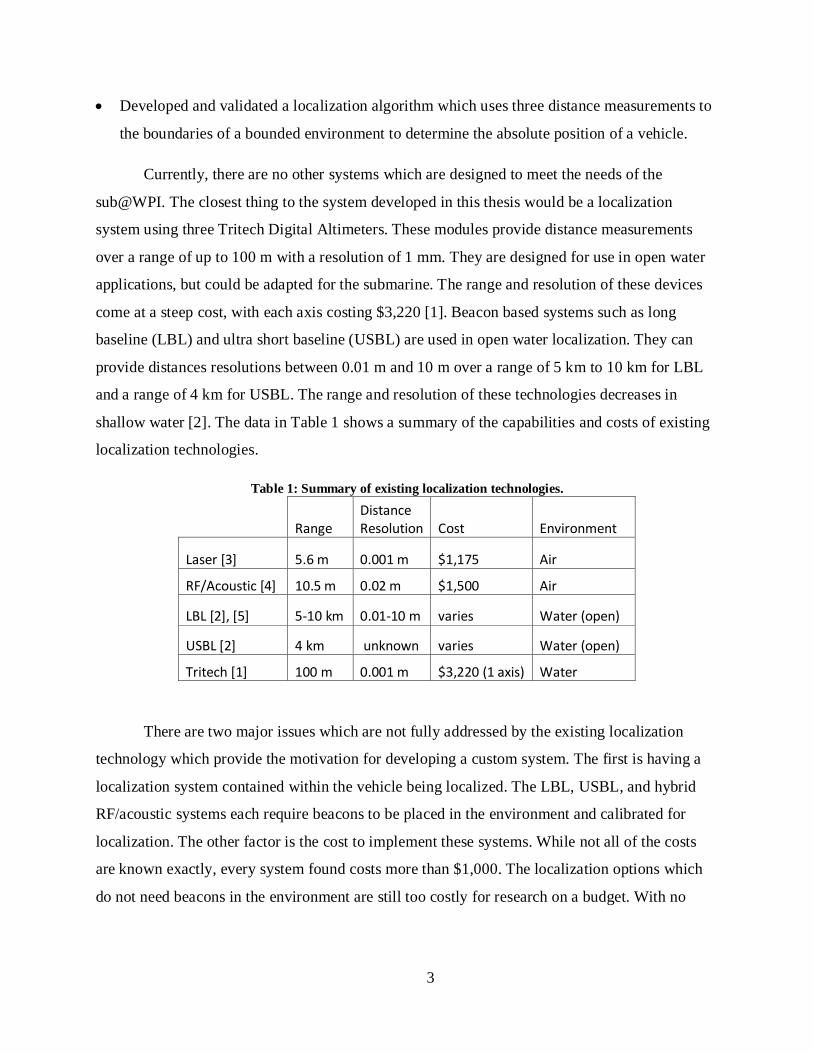
shallow water [2]. The data in Table 1 shows a summary of the capabilities and costs of existing
localization technologies.
Table 1: Summary of existing localization technologies.
Range
Distance Resolution Cost Environment
Laser [3] 5.6 m 0.001 m $1,175 Air
RF/Acoustic [4] 10.5 m 0.02 m $1,500 Air
LBL [2], [5] 5-10 km 0.01-10 m varies Water (open)
USBL [2] 4 km unknown varies Water (open)
Tritech [1] 100 m 0.001 m $3,220 (1 axis) Water
There are two major issues which are not fully addressed by the existing localization
technology which provide the motivation for developing a custom system. The first is having a
localization system contained within the vehicle being localized. The LBL, USBL, and hybrid
RF/acoustic systems each require beacons to be placed in the environment and calibrated for
localization. The other factor is the cost to implement these systems. While not all of the costs
are known exactly, every system found costs more than $1,000. The localization options which
do not need beacons in the environment are still too costly for research on a budget. With no
4
clear option for self-contained localization at a reasonable price, a custom system was developed
to meet that need.
This thesis details the development of a custom, ultrasonic, localization module for
autonomous underwater vehicles. Chapter 2 discusses the existing localization systems and
methods employed by other researchers. The design and fabrication of the electronics for the
sonar module is detailed in Chapter 3. Chapter 4 is about the debugging and testing done after
receiving the fabricated boards and while developing the signal processing techniques that would
be used. Chapter 5 explains the signal processing methods used to measure distances with the
ultrasonic pulses. The derivation of the algorithm to be implemented on the submarine is
explained in Chapter 6. It uses the distance measurements from the sonar module to calculate its
position. The design and construction of the sensor housing is discussed in 7. The results of the
initial localization testing are presented in Chapter 8. Chapter 9 offers conclusions based upon
the work and Chapter 10 has recommendations and future work to be completed.

5
2 Localization Systems and Methods Localization is a classic problem in the field of robotics, and without accurate location
information, robots would be greatly limited in the tasks they perform. A wide variety of
solutions exist for robotic localization, however they are not suited for all applications.
Localization systems can be grouped into two major categories. Passive localization systems
gather information from their environment or beacons placed within their environment and active
systems transmit energy into their environment and measure the effect. This chapter discusses
the positioning systems in use for robotic systems. After explaining the state of the art, the need
for the system developed in this thesis is explained.
2.1 Passive Localization Systems Passive localization systems do not transfer energy to their environment for the purpose
of localization, but rather use sensors to measure their surroundings. There are a number of
different passive sensing systems, among which are deduced reckoning, beacon-based
navigation, and vision-based navigation.
2.1.1 Deduced Reckoning
Deduced reckoning, or dead reckoning as it is often called, is sometimes used as a means
of robot localization. The robot begins at a known starting point and uses assumptions about the
vehicle’s dynamics to figure out its position relative to the starting location. If the robot
dynamics do not exactly follow the computer model, this method alone can lead to large errors in
position measurements. Dead reckoning is often used in conjunction with sensors on the vehicle
which measure things such as distance traveled, velocity, and acceleration. These dynamically
fused measurements can produce more accurate localization.
2.1.2 Inertial Navigation
An inertial navigation system measures the accelerations of a vehicle and uses this data to
calculate the movements of the vehicle relative to its previously known position. The
acceleration measurements are integrated with respect to time to find the vehicle velocity and
then again to get position. The double integration causes large errors in the position estimates to
accumulate very quickly. The actual sensor, an inertial measurement unit or IMU, is also
expensive compared to other sensor options and has a high rate of drift [6].

6
Inertial navigation systems are the most successful when combined with other sensors
because the other sensor values can be used to reset the integration of the IMU and stop the error
from growing unbounded. One such implementation described in [7] uses an IMU with GPS and
an acoustic positioning system. A Kalman filter is used to provide the best estimate of the
vehicle location given the three potentially conflicting sensor values.
2.1.3 Beacon-Based Localization
Many robotic systems employ a set of beacons placed throughout the environment for
localization. These beacons are at specific locations which are known to the robot. The beacons
transmit signals which are received by the robot and used to calculate the distance between the
robot and each beacon. With the information about the position of the beacons and their
respective distances from the robot, the receiver can analytically determine its location in 2D or
3D space. The process of determining a robots location in this manner is known as trilateration
and is explained in [8]. Essentially, trilateration calculates the intersection point of theoretical
spheres with centers located at each beacon and with radii equal to the distances to each beacon.
2.1.3.1 Global Positioning System
Likely the most well known beacon based positioning system, the Global Positioning
System or GPS, is a widely used method for localization for surface based robotics. A network of
24-32 satellites orbits the Earth in medium earth orbit and broadcast their locations periodically
to receivers on the ground. Each broadcast signal is sent with a time stamp and the location of
the satellite so the receiver can determine the time-of-flight of the signal and use it to calculate
the distance. If 4 or more different signals are received, the receiving unit can calculate its
position on the surface to within a few meters.
With uncertainties of several meters, a small scale robot which employs GPS alone will
have difficulty moving in a complex environment. Also, the path loss of the GPS signals through
water is such that they cannot be detected more than a few centimeters beneath the water. GPS
has been implemented for underwater localization in [9] by using it to locate a surface vehicle
which then located the underwater vehicles and beacons relative to its position using acoustic
sensors.
7
A number of different localization systems have been developed which have reasonable
resolutions on a small scale. Many of these systems were developed to simulate GPS in a
laboratory environment. Some of these systems have been adapted for use with underwater
vehicles.
2.1.3.2 Acoustic Beacons
A passive acoustic localization system can be achieved by placing acoustic sources in
fixed locations within the environment and measuring their position relative to the robot. The
method outlined in [10] uses multiple microphones placed at different locations on the robot. The
sound from the beacons arrives at each microphone at different times and the relative time
difference can be used to determine the position of the source.
Other implementations of this type do not require beacons at all. Instead, the passive
sonar system developed in [11] makes use of ambient noise in its surroundings for localization.
Like the previous paper, it uses multiple separate detectors to determine the time delay of arrival,
abbreviated as TDOA. The arrival information is used to calculate the angle from which the
signal came and the signal strength is used to estimate the range. A system such as this could
potentially be implemented on the sub@WPI, but the need for multiple maneuverable sensors
would increase the complexity and cost for accurate, low-budget localization purposes.
2.1.3.2.1 Hybrid RF/Acoustic Localization
The Cricket Indoor Localization System was developed at the Massachusetts Institute of
Technology and uses a combination of radio frequencies and acoustic sensors for localization.
The system uses the difference in speeds between radio and acoustic waves to measure the time
of flight. Both pulses are sent at the same time from a Cricket beacon. The radio pulse arrives at
the Cricket listener almost instantly compared to the time of flight for the sound. When the radio
pulse arrives, the system starts a timer which counts until the corresponding acoustic pulse is
received. With this method, there is no need for the transmitter and receiver to be synchronized
as with GPS [4].
Researchers at the Universities of Wyoming and Eastern Oregon developed a multi-robot
localization scheme which uses hardware similar to that provided by MIT’s Cricket system. This
system calculates the distances between agents within a network of robots and uses trilateration
8
to determine their relative locations. These locations are used to control the robots and keep them
in prescribed formations during operations [12].
2.1.4 Vision-Based Localization
Some positioning systems use digital cameras to gather information about a vehicle’s
surroundings in order to determine its relative position. One such method presented in [13], [14]
captures images below the robot as it moves through the environment. Landmarks within the
images are used to match overlapping images and create a single representation of the domain.
Once the map of the domain has been generated, the computer can compare incoming images to
the mosaic and determine its location. This approach is susceptible to varying light conditions.
Also, the relative homogeneity of the imaged surface is a major factor in its success because of
the need to overlap images.
Another implementation of a visual localization system similar to those above is detailed
in [15]. It uses a combination of vision sensors and inertial sensors to perform simultaneous
localization and mapping, abbreviated SLAM. The use of additional sensor information with the
video allows the robot to continue localization when the position determined from the video
alone is uncertain.
The localization system developed in [16] compares images taken with two video
cameras. The processor identifies a series of landmarks which occur in both images. If these
landmarks appear in successive sets of images, their relative positions within each image can be
used to calculate their three dimensional position. This approach assumes that the robot is
moving at a constant velocity in order to determine the relative distance moved between frames.
Evolution Robotics, Inc. has developed a different type of passive vision based
localization system which uses infrared sources as beacons and a proprietary detector as a
receiver [17]. The infrared sources are projected like spotlights onto a surface within the
environment. Each source has an individual ID which can be determined by the robot. The
detector on the robot measures the location and heading direction of the visible beacons and uses
that information to triangulate its location in the environment [17].
9
2.2 Active Localization Active localization systems actively emit energy into their environment and measure the
response to this energy to determine their location. Due to their nature, these types of systems are
only used when vehicle stealth is not critical. There are a multitude of active localization
methods available, among which are electrolocation, radar, laser scanners, active vision, and
active acoustic ranging. This section describes these methods and examines their suitability for
localization of the sub@WPI submarine.
2.2.1 Electrolocation
Some research groups have begun testing systems which use electrolocation for
determining position. Electrolocation is inspired by certain types of fish which have been found
to emit a weak electric field for detecting objects. Objects in close proximity to the fish will
cause detectable disturbances in the electric field. The system developed in [18] uses a robot with
four electrodes, two for producing the electric field and two for receiving. The electrical
conductivity of the water is an important factor with this system, though it has been proven to
work in both fresh and salt water situations. The electrolocation experiments were conducted
under very controlled conditions in a laboratory over a relatively short range. This approach is
currently not suitable for mobile robot localization; however, it is an interesting area of research.
2.2.2 Radar
One of the oldest methods of active localization is radar, which stands for Radio
Detection and Ranging. In the years leading up to World War 2, several independent groups
were working to develop radar systems to use as a warning system for incoming aircraft. Radar
was successfully demonstrated in the 1920s, but the impending war was a catalyst for increased
development funding. A radio wave of a known wavelength is transmitted and a receiver listens
for an echo from that signal bouncing off a target. The wavelength of the transmitted pulse limits
the resolution of the measured range. Some of the early systems were only able to detect if a
target was present using interference between the received and transmitted signal, but they could
not determine the range or location of the target [19].
Since its early beginnings, radar has been greatly improved and has been adapted for
some robotic applications. A team at Carnegie Mellon University used a millimeter wavelength
radar system for short range localization and mapping measurements in [20]. Researchers at the
10
Australian Centre for Field Robotics developed a custom millimeter wavelength radar system to
be used on an unmanned aerial vehicle [21]. Millimeter wave radar has also been used to
implement a SLAM algorithm as presented in [22].
The main problem with using radar as a means of localization in an underwater
environment is the tradeoff between range and resolution. The millimeter wave radar systems
used for the projects described above would be attenuated quickly in water because of their
relatively high frequency. Longer wavelength radar could be used, but it would only provide
very coarse distance measurement capability. Coarse distance measurements would not be useful
for a small-scale localization system.
2.2.3 Laser scanners
Another method of active localization is the use of a laser range finder or laser scanner. A
laser is shined on the environment and precision electronics measure the time it takes for the
light to return. By scanning around the robot over a range of angles, a map of surrounding area
can be developed. This map can either be used to localize the robot based on an existing map or
to develop a map as the robot moves using an algorithm like SLAM. Laser scanners have the
advantage of being highly accurate. However, commercially available laser scanners can be
prohibitively expensive. Examples of the costs are the Hokuyo UTM-30LX laser scanner for
$5590 [23] and the lower range Hokuyo URG-04LX-UG01 laser scanner for $1175 [3].
Laser scanning systems have been implemented for underwater applications. In [24] a
custom system was developed which uses laser pointers and a color digital camera. The vehicle
is held stationary while the laser pointers are scanned over an object and successive images are
captured. The orientation of the laser pointers is used to triangulate the location of the point of
reflection relative to the vehicle in each image. The individual points are then used to develop a
map of the environment. This system is heavily dependent on the clarity of the water and the
available light [24].
2.2.4 Active Vision Systems
An active vision system shines a light source on its environment and measures the
response. The light used is not necessarily in the visible spectrum. Often infrared is used in

11
situations where visible light would hinder the performance of the system. Infrared is also used
for stealth reasons when visible light would alert casual observers of the vehicles presence.
One of the simplest forms of active vision systems is an infrared proximity detector. An
infrared source is shined on a target surface and the reflection is measured with a photodiode.
The intensity of the reflected light corresponds with the distance to the reflecting surface. These
sensors are limited in their use for localization because they have a relatively short range and are
highly sensitive to other sources of infrared light, such as the sun. Also, wavelengths in the
infrared portion of the spectrum would not be ideal or use underwater because they are absorbed
by the water.
A Korean company called Hagisonic has developed an active vision based positioning
system which is commercially available. The Hagisonic StarGazer system illuminates spatially
placed reflectors with infrared lights and records their location in an image captured with an
onboard CCD. Each reflector has a unique series of dots which allows it to be identified in the
image. Other dots on the reflector serve to provide orientation information so the robot can
determine the heading to the reflector. Using the heading information and the image taken by the
CCD, the system can return the robot position relative to the reflector [25]. A system such as this
could be used underwater, but it would be greatly dependent on the clarity of the water. Also, as
stated above, the infrared light used to illuminate the reflectors would be quickly absorbed
underwater which would greatly limit its range.
2.2.5 Active Acoustic Ranging
One of the most prevalent forms of localization in underwater environments is the use of
active acoustic ranging, also known as sonar. Active acoustic ranging systems can be
implemented in a variety of different configurations, several of which are presented in this
section.
The method described in [26] uses an active ultrasonic ranging system to measure the
environment around the robot. The robot uses six static ultrasonic sensors to cover all the area
around the robot. The distance measurements are used to create a map of the surrounding area.
One of the major shortcomings of an ultrasonic ranging sensor is that the transmitted pulse is not
always reflected directly back to the receiver, particularly when the angle between the sensor

12
axis and the reflector is small. If the signal does eventually return to the receiver by multi-path
reflection, an incorrect distance measurement is recorded. To account for these inevitable errors
in measurement, certain data processing techniques are employed. Leonard and Durrant-Whyte
utilize an Extended Kalman Filter to compare the expected location of the vehicle with the
measured location and use this comparison to estimate the robot position. The Kalman filter
estimate allows a map to be constructed as the robot moves in a SLAM algorithm. The problem
with applying a similar approach to this research for the submarine is that it relies on discrete
landmarks extracted from the generated maps for localization [26]. The ultrasonic localization
system presented in this thesis would effectively use the entire boundary of the environment for a
SLAM implementation.
Two popular approaches to active acoustic localization are long baseline (LBL) and ultra-
short baseline (USBL). An LBL system is given this name because it uses multiple beacons or
transponders with a long distance between them, known as the baseline. It contrasts with USBL
configurations in which sensors placed near each other on a single surface vessel and the position
of each is determined with GPS. For LBL, the beacons can either be placed in static locations for
confined testing or dragged on a line behind a surface vehicle in open water applications. When
pulled behind a moving vessel, the onboard GPS is used to provide the absolute location of the
beacons. With both configurations, the AUV transmits a signal which is received by a beacon
and the beacon in turn transmits a response back to the AUV. The time of flight is measured and
used to calculate the range to the transponder. Though this type of system employs beacons or
transponders, it is not a passive localization system because the robot actively sends signals to
the beacons for localization. In [27], a custom LBL system is implemented which is fused with
vehicle velocity data to implement a Kalman filter. The research presented in [2], considers the
benefits of a few different types of localization systems including LBL and USBL systems.
While these systems are usually thought of on a kilometer scale, they could be implemented in a
smaller test environment. One of the major drawbacks to either system is the need for calibrating
and localizing the beacons followed by calibrating the AUV to the beacons. A SLAM algorithm
could be performed if the calibration were not done, but this would not provide the best
positioning data [2].

13
Researchers have also worked to improve the performance of LBL systems by combining
LBL with other sensors. One such AUV project, described in [5], uses a combination of LBL and
Doppler-based navigation. The Doppler-based navigation method measures the frequencies of
echoed ultrasonic pulses and uses the difference in frequency between the transmitted and
received signals to determine the vehicle velocity in the direction the pulse was sent. By
combining the velocity measurements with an LBL localization system, they were able to
produce more accurate localization results [5].
The mobile robot described in [28] uses a scanning ultrasonic sensor to measure the
distances to the nearest object 360 degrees around itself. These scans are used to localize the
robot on a known map based on the detected landmarks. The scans require filtering because
when the ultrasonic transducer is not nearly perpendicular with a reflecting surface, the signal
will not travel directly back to the sensor, and any received echo yields a distance much longer
than in actuality. The landmarks are extracted primarily by finding straight lines within the scans
which correspond to the edges of landmarks. If enough lines are detected, the robot can uniquely
calculate its position in the environment [28].
A commercially available underwater ultrasonic distance measurement system is sold by
Tritech International. This system operates at either 200 or 500 kHz and offers ranges at 100 and
50 meters respectively. The Tritech PA200 and PA500 Digital Altimeters both have a resolution
of 1 mm for distance measurements. This alone would make them an ideal solution for
localization of the sub@WPI. However, each unit costs $3220 which is far outside the budget for
this project, especially where three units would be needed for localization [1].
2.2.5.1 Challenges to Active Acoustic Ranging
While widely used for localization, acoustic ranging is by no means a perfect solution to
the positioning problem. When an ultrasonic transducer is placed perpendicular to a flat surface,
it is highly likely that a signal will reflect off the surface directly back to the sensor. As the angle
between the sensor and the reflecting surface deviates from perpendicular, the likelihood that the
signal will not be reflected directly back to the sensor increases. The performance at these angles
is better for textured reflecting surfaces, but they will still not yield accurate results at all angles.
14
If the transmitted signal does not immediately return to the sensor, one of two things can
happen. One possible track is that it could continue reflecting around the environment and never
return to the sensor before it has attenuated. In this case the software will trigger a timeout when
no response is seen after a given interval. The other possibility is that the signal reflects off of
two or more surfaces and then finds its way back to the transducer. For this situation the
algorithm will calculate a larger distance to the boundary than in actuality. These distance
measurement errors could lead to substantial errors in the calculated position of a robot.
2.3 Need for a Custom Localization System
Several of the localization systems described in the previous section have been tested and
proven underwater; however, no currently available localization system was sufficient to meet
the unique needs of the sub@WPI AUV. Beacon based passive localization systems were ruled
out early in the decision making process because one of the desired features was a lack of
external hardware needed for localization. The use of odometry and inertial measurements was
discarded because of the potential for accumulated errors due to drift. A vision based system was
considered, but it was considered too complicated to implement in an environment with few
distinctly identifiable landmarks to use as references.
This left only the active localization systems to choose from. Radar and electrolocation
were dismissed because they are infeasible for our application. The high cost of a laser scanner
and the need for relatively high water clarity to measure long distances removed them from the
running. Only active acoustic localization remained as a means for positioning the submarine.
None of the existing systems were especially suited for the needs of the sub@WPI. Because of
this, it was decided that a custom self-contained active acoustic ranging system would be built
for localization of the sub@WPI. The system is made of an inexpensive custom circuit board and
off-the-shelf components, so it is much more economical than comparable systems. Also, it does
not require the additional time to setup and calibrate a network of beacons each time the
submarine will be operated which makes more efficient use of the allotted pool testing time.
15
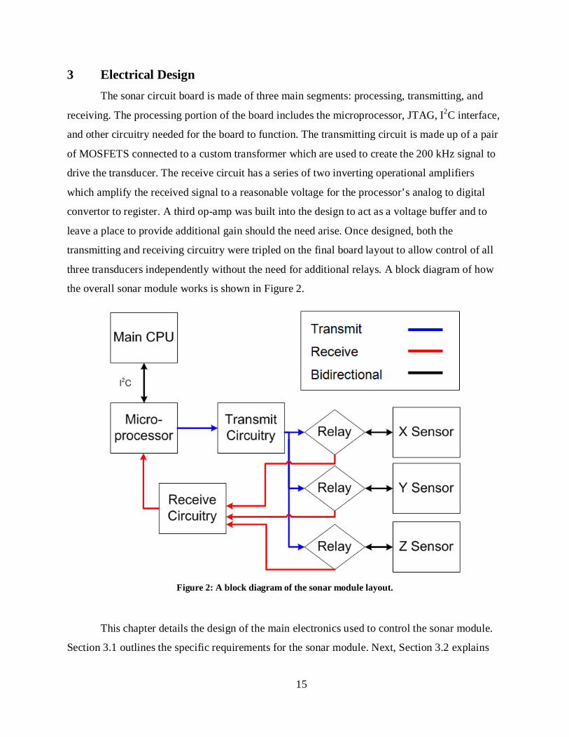
3 Electrical Design The sonar circuit board is made of three main segments: processing, transmitting, and
receiving. The processing portion of the board includes the microprocessor, JTAG, I2C interface,
and other circuitry needed for the board to function. The transmitting circuit is made up of a pair
of MOSFETS connected to a custom transformer which are used to create the 200 kHz signal to
drive the transducer. The receive circuit has a series of two inverting operational amplifiers
which amplify the received signal to a reasonable voltage for the processor’s analog to digital
convertor to register. A third op-amp was built into the design to act as a voltage buffer and to
leave a place to provide additional gain should the need arise. Once designed, both the
transmitting and receiving circuitry were tripled on the final board layout to allow control of all
three transducers independently without the need for additional relays. A block diagram of how
the overall sonar module works is shown in Figure 2.
Figure 2: A block diagram of the sonar module layout.
This chapter details the design of the main electronics used to control the sonar module.
Section 3.1 outlines the specific requirements for the sonar module. Next, Section 3.2 explains

16
the previous work done by last year’s MQP group to create the initial design for the sonar board.
That section also lists some of the remaining challenges still facing the project after the MQP.
Sections 3.3-3.6 explain the design work and simulations performed to finalize the board design.
The preparations to have the boards fabricated are detailed in Section 3.7. Section 3.8 discusses
the costs incurred for the development of the sonar module.
3.1 Sonar Module Requirements
The sonar module described in this thesis needed to meet certain requirements which
were not met by any of the previously existing localization methods outlined in Chapter 2. The
first major requirement is that the sonar system must be self contained within or attached to the
AUV. Any additional hardware setup would subtract from the overall research time allotted with
setup and cleanup time. Secondly, the module must be made from off the shelf components
whenever possible, with the exception of a custom circuit board, to reduce complexity and save
time. The module should be able to determine the three dimensional location of the AUV to
within 0.20 m of its absolute location. The minimum measurable distance must be no greater
than 1.00 m and the module should be capable of measuring distances up to 20.00 m. Finally, the
module must fit within the budget of the sub@WPI project and should not cost more than $500
to build.
3.2 Previous Work During the 2008 academic year, a group of WPI students worked on the design and
fabrication of an autonomous submarine to be used for research and development of search
algorithms for their Major Qualifying Project. Part of their work was the initial design and
development of the circuitry for an ultrasonic positioning system. This system would allow the
submarine to determine its three-dimensional location within a pool or tank and use that data in
control feedback loops to execute complex algorithms. This section briefly explains the
architecture of the sub@WPI and then details the previous work performed on the development
of the sonar module.
3.2.1 Submarine Architecture
The sub@WPI submarine is 1.2 m long, 0.6 m in height, and 0.7 m wide. It contains two
ballast tanks, fore and aft, to regulate its depth and stability. A central pump supplies these tanks
and also provides water for four water jets on the corners of the submarine. These water jets are
17
used to dynamically stabilize the submarine. Locomotion for the submarine is provided by two
custom thrusters. The thrusters use magnetic couplings to drive the propellers so no dynamic
sealing is needed to keep water out of the motors [29].
The sub@WPI is controlled by a PC/104 embedded computer running a Linux operating
system. A 16 channel data acquisition board is connected to the PC/104 to read the sensors on
the submarine. These sensors include a pressure sensor, temperature sensor, a custom leak
sensor, a battery voltage sensor, and the sonar module. The water jets and ballast tanks are
regulated by solenoid valves. The solenoid valves and motors are controlled by second custom
circuit board [29].
3.2.2 Sonar Module
To begin with, the group constructed a simple setup using 40 kHz air-based ultrasonic
transducers as a test platform. The proposed sensor would be measuring the time that it takes for
a transmitted pulse to be returned to the same transducer as an echo. Because these are such time
sensitive measurements, a dedicated microprocessor was chosen to transmit, measure, and
process the ultrasonic signals before sending them to the central PC/104. Initially, the
transducers were connected to an oscilloscope to measure the signals. During later experiments,
a PC was used in place of the submarine’s central processor so the measured signals could be
analyzed and plotted using MATLAB [29].
After working with these air-based transducers and performing several experiments, it
was determined that they did not transmit enough power to be effective underwater over any
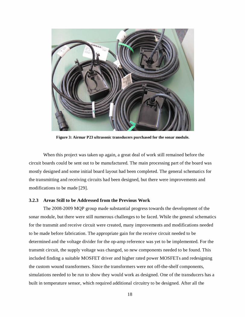
reasonable distance. The team decided to pursue a transducer traditionally used for commercially
available fish finding systems because they are already known to function well underwater. The
Airmar P23 transducer was chosen for its size, price, and the detailed specifications available
from the manufacturer which aided with design. An image of the transducers purchased for the
sonar module can be seen in Figure 3. In normal operation, the Airmar transducers are controlled
by an electronic fish finder which generates the 200 kHz pulse, amplifies the received signal, and
processes the signal to determine if there are fish within the sensor’s beam. The sonar module
needed to be designed to perform all these tasks and communicate its measurements to the rest of
the submarine [29].
18
Figure 3: Airmar P23 ultrasonic transducers purchased for the sonar module.
When this project was taken up again, a great deal of work still remained before the
circuit boards could be sent out to be manufactured. The main processing part of the board was
mostly designed and some initial board layout had been completed. The general schematics for
the transmitting and receiving circuits had been designed, but there were improvements and
modifications to be made [29].
3.2.3 Areas Still to be Addressed from the Previous Work
The 2008-2009 MQP group made substantial progress towards the development of the
sonar module, but there were still numerous challenges to be faced. While the general schematics
for the transmit and receive circuit were created, many improvements and modifications needed
to be made before fabrication. The appropriate gain for the receive circuit needed to be
determined and the voltage divider for the op-amp reference was yet to be implemented. For the
transmit circuit, the supply voltage was changed, so new components needed to be found. This
included finding a suitable MOSFET driver and higher rated power MOSFETs and redesigning
the custom wound transformers. Since the transformers were not off-the-shelf components,
simulations needed to be run to show they would work as designed. One of the transducers has a
built in temperature sensor, which required additional circuitry to be designed. After all the
19
schematics were updated, the components needed to be individually placed on the circuit board
and each wire routed to connect appropriately.
The previous work was focused on the electrical design of the sonar module and did not
delve into the signal processing or localization algorithm aspects of the problem. An innovative
method for processing the received signal within the limitations of the hardware needed to be
designed. The signal processing methodology is outlined in Chapter 5. Once a received signal is
processed and a measured distance is output from the sonar module, the AUV needs to use this
data to determine its location. A custom localization algorithm was developed to determine the
position of the submarine using the three measured distances and the measured orientation of the
submarine. The details of the localization algorithm are explained in Chapter 6.
The packaging or mounting of the sonar module was not addressed by the previous work.
A compact mounting bracket was designed to mount the sensors orthogonally and conform to the
submarine’s unique hull shape. The mechanical aspects of the sonar module design are discussed
in Chapter 7.
3.3 Sonar Signal Processing Circuit
The sonar module is based around the MSP430F2410 low power microprocessor
manufactured by Texas Instruments. The module was designed with a separate processor from
the main PC/104 because the ultrasonic measurements are highly time sensitive. Regardless of
the current subroutine being performed by the PC/104, the separate microprocessor on the sonar
board can update its position measurements without interrupting other submarine functions. The
sonar module is able to obtain sonar readings independently of the main processor and can
supply data to the processor as it is requested.
At each point on the sonar module where the voltage is critical, including the reference
voltage and power connections, they are two decoupling capacitors connected between that point
and ground. Though a casual observer may think these components are extraneous, they are
important to the operation of the circuit. The capacitors isolate noise in different sections of the
board to keep it from interfering with other sections. This allows us to use a single ground plane
for AC and DC instead of keeping them separate.
20
The general purpose digital input/output pins available on the MSP430 are used to
control the transmit circuitry. The MSP430 has two analog to digital convertors built into the
processor itself. The higher precision 12-bit ADC, which is often called ADC12, was chosen to
process the signals from the receive circuit. Each channel of the receive circuit is connected to
one of the analog input pins assigned to this ADC.
Once the signal has been transmitted, received, and processed by the MSP430, the
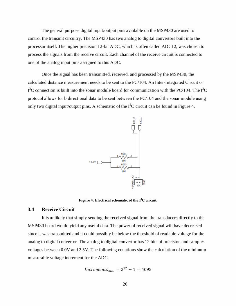
calculated distance measurement needs to be sent to the PC/104. An Inter-Integrated Circuit or
I2C connection is built into the sonar module board for communication with the PC/104. The I2C
protocol allows for bidirectional data to be sent between the PC/104 and the sonar module using
only two digital input/output pins. A schematic of the I2C circuit can be found in Figure 4.
Figure 4: Electrical schematic of the I2C circuit.
3.4 Receive Circuit It is unlikely that simply sending the received signal from the transducers directly to the
MSP430 board would yield any useful data. The power of received signal will have decreased
since it was transmitted and it could possibly be below the threshold of readable voltage for the
analog to digital convertor. The analog to digital convertor has 12 bits of precision and samples
voltages between 0.0V and 2.5V. The following equations show the calculation of the minimum
measurable voltage increment for the ADC.
𝐼𝐼𝐼𝐼𝐼𝐼𝐼𝐼𝐼𝐼𝐼𝐼𝐼𝐼𝐼𝐼𝐼𝐼𝐼𝐼𝐴𝐴𝐴𝐴𝐴𝐴 = 212 − 1 = 4095
21
𝑉𝑉𝑉𝑉𝑉𝑉𝐼𝐼𝐼𝐼𝐼𝐼𝐼𝐼𝐼𝐼𝐼𝐼𝐼𝐼𝐼𝐼𝐼𝐼𝐼𝐼𝐼𝐼𝐼𝐼
=2.5𝑉𝑉4095
= 611𝜇𝜇𝑉𝑉
To make sure that the signals received are above this minimum, operational amplifiers
are employed to amplify the signal voltage to a more desirable level. An operational amplifier is
an integrated circuit made of several transistors and other components. The sonar module uses
the op-amps in the inverting op-amp configuration; however, they are useful for a large array of
practical applications [30].
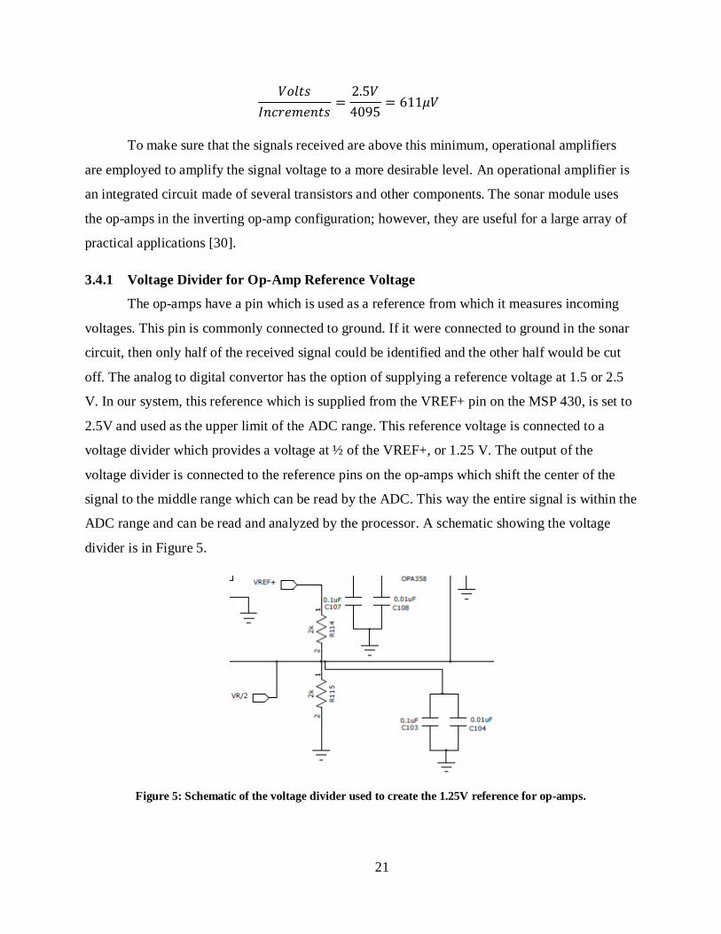
3.4.1 Voltage Divider for Op-Amp Reference Voltage
The op-amps have a pin which is used as a reference from which it measures incoming
voltages. This pin is commonly connected to ground. If it were connected to ground in the sonar
circuit, then only half of the received signal could be identified and the other half would be cut
off. The analog to digital convertor has the option of supplying a reference voltage at 1.5 or 2.5
V. In our system, this reference which is supplied from the VREF+ pin on the MSP 430, is set to
2.5V and used as the upper limit of the ADC range. This reference voltage is connected to a
voltage divider which provides a voltage at ½ of the VREF+, or 1.25 V. The output of the
voltage divider is connected to the reference pins on the op-amps which shift the center of the
signal to the middle range which can be read by the ADC. This way the entire signal is within the
ADC range and can be read and analyzed by the processor. A schematic showing the voltage
divider is in Figure 5.
Figure 5: Schematic of the voltage divider used to create the 1.25V reference for op-amps.
22
3.5 Transmit Circuit The transmit circuit had the most amount of work remaining to be done. Each channel of
the transmit circuit makes use of three digital input/output pins from the MSP430
microprocessor. One of the pins is used to trigger the relay to be connected to the secondary side
of the transformer so a signal can be transmitted. Since the transducer would draw an immense
amount of power if it were run at a high duty cycle, the relay used was configured to be normally
connected to the receive circuit. Whenever a pulse needs to be transmitted, the trigger pin is
turned on briefly to connect it to the transducers, then the relay switches back to receive mode to
capture the corresponding echo.
The other two pins are used to control two power MOSFETs which are used to create the
driving signal for the transducer. Between the microprocessor and the MOSFETs is a MOSFET
driving integrated circuit which does the actual driving of the MOSFETs. The driving IC is used
to control the MOSFETs because the pins on the microcontroller output 3.3 volts when they are
in a high position and the MOSFETs are designed to be switched with 5.0 volts.
The MOSFETs are used in unison to control the flow of current through a custom built
transformer. The transformer has a center-tap on the primary coil side. This center tap allows the
direction of current flow in the secondary coil to be switched depending on which MOSFET is
turned on. The MOSFETs are turned on and off out of phase from each other to generate a 200
kHz pulse.
3.5.1 Change from 24 Volts Supply to 12 Volts
The original transmit circuit designed by the MQP group required a 24V supply from the
submarine. This was chosen for convenience because at that point there were other major
components of the submarine which required 24V to operate. Since then, the submarine design
was further optimized as to eliminate all other needs for a 24V supply. With the 24V supply no
longer a convenient choice for the sonar module, the design was modified to run on a 12V supply
which can be obtained directly from the batteries.
The original transformer was made to deliver 200 Watts to the ultrasonic transducer, and
this specification was held with the new transformer. The process used by the MQP group to
23
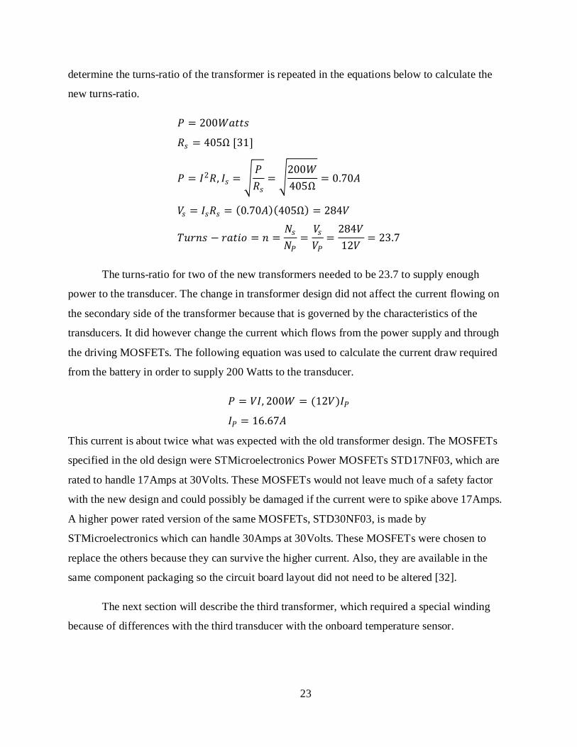
determine the turns-ratio of the transformer is repeated in the equations below to calculate the
new turns-ratio.
𝑃𝑃 = 200𝑊𝑊𝑊𝑊𝐼𝐼𝐼𝐼𝐼𝐼
𝑅𝑅𝐼𝐼 = 405Ω [31]
𝑃𝑃 = 𝐼𝐼2𝑅𝑅, 𝐼𝐼𝐼𝐼 = 𝑃𝑃𝑅𝑅𝐼𝐼
= 200𝑊𝑊405Ω
= 0.70𝐴𝐴
𝑉𝑉𝐼𝐼 = 𝐼𝐼𝐼𝐼𝑅𝑅𝐼𝐼 = (0.70𝐴𝐴)(405Ω) = 284𝑉𝑉
𝑇𝑇𝑇𝑇𝐼𝐼𝐼𝐼𝐼𝐼 − 𝐼𝐼𝑊𝑊𝐼𝐼𝑟𝑟𝑉𝑉 = 𝐼𝐼 =𝑁𝑁𝐼𝐼𝑁𝑁𝑃𝑃
=𝑉𝑉𝐼𝐼𝑉𝑉𝑃𝑃
=284𝑉𝑉12𝑉𝑉
= 23.7
The turns-ratio for two of the new transformers needed to be 23.7 to supply enough
power to the transducer. The change in transformer design did not affect the current flowing on
the secondary side of the transformer because that is governed by the characteristics of the
transducers. It did however change the current which flows from the power supply and through
the driving MOSFETs. The following equation was used to calculate the current draw required
from the battery in order to supply 200 Watts to the transducer.
𝑃𝑃 = 𝑉𝑉𝐼𝐼, 200𝑊𝑊 = (12𝑉𝑉)𝐼𝐼𝑃𝑃
𝐼𝐼𝑃𝑃 = 16.67𝐴𝐴
This current is about twice what was expected with the old transformer design. The MOSFETs
specified in the old design were STMicroelectronics Power MOSFETs STD17NF03, which are
rated to handle 17Amps at 30Volts. These MOSFETs would not leave much of a safety factor
with the new design and could possibly be damaged if the current were to spike above 17Amps.
A higher power rated version of the same MOSFETs, STD30NF03, is made by
STMicroelectronics which can handle 30Amps at 30Volts. These MOSFETs were chosen to
replace the others because they can survive the higher current. Also, they are available in the
same component packaging so the circuit board layout did not need to be altered [32].
The next section will describe the third transformer, which required a special winding
because of differences with the third transducer with the onboard temperature sensor.
24
3.5.2 Special Transformer Winding for Second Transducer Type
As mentioned in the previous section, only two of the transformers matching windings.
While making the adjustment in transformer winding to account for the change in power supply,
it was discovered that the sensors purchased did not all have identical electrical characteristics.
One of the three transducers has a built in temperature sensor and correspondingly has a different
equivalent resistance. Below the same calculations performed for the first transformed are
recalculated for the second transformer.
𝑃𝑃 = 200𝑊𝑊𝑊𝑊𝐼𝐼𝐼𝐼𝐼𝐼
𝑅𝑅𝐼𝐼 = 525Ω [33]
𝑃𝑃 = 𝐼𝐼2𝑅𝑅, 𝐼𝐼𝐼𝐼 = 𝑃𝑃𝑅𝑅𝐼𝐼
= 200𝑊𝑊525Ω
= 0.62𝐴𝐴
𝑉𝑉𝐼𝐼 = 𝐼𝐼𝐼𝐼𝑅𝑅𝐼𝐼 = (0.617𝐴𝐴)(525Ω) = 324𝑉𝑉
𝑇𝑇𝑇𝑇𝐼𝐼𝐼𝐼𝐼𝐼 − 𝐼𝐼𝑊𝑊𝐼𝐼𝑟𝑟𝑉𝑉 = 𝐼𝐼 =𝑁𝑁𝐼𝐼𝑁𝑁𝑃𝑃
=𝑉𝑉𝐼𝐼𝑉𝑉𝑃𝑃
=324𝑉𝑉12𝑉𝑉
= 27
The resistance of the second type of transducer is higher and which means less current
flows through it for a given power. This gives a correspondingly higher voltage drop across the
sensor and leads to the higher turns-ratio of 27.
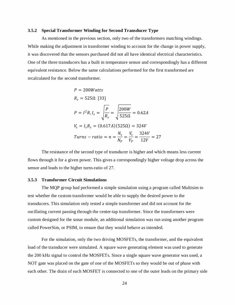
3.5.3 Transformer Circuit Simulations
The MQP group had performed a simple simulation using a program called Multisim to
test whether the custom transformer would be able to supply the desired power to the
transducers. This simulation only tested a simple transformer and did not account for the
oscillating current passing through the center-tap transformer. Since the transformers were
custom designed for the sonar module, an additional simulation was run using another program
called PowerSim, or PSIM, to ensure that they would behave as intended.
For the simulation, only the two driving MOSFETs, the transformer, and the equivalent
load of the transducer were simulated. A square wave generating element was used to generate
the 200 kHz signal to control the MOSFETs. Since a single square wave generator was used, a
NOT gate was placed on the gate of one of the MOSFETs so they would be out of phase with
each other. The drain of each MOSFET is connected to one of the outer leads on the primary side
25
of the transformer and the source of each MOSFET is connected to ground. A constant DC
voltage supply was connected to the center tap on the transformer. A resistor representing the
equivalent resistance of the transducer was placed on the secondary side of the transformer. With
the circuit completed, special measurement elements were added to measure the voltage and
current at various locations in the circuit. A screenshot of the simulation schematic can be found
in Figure 6.
Figure 6: The schematic layout of the PSim simulation for the custom transducer.
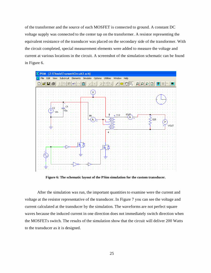
After the simulation was run, the important quantities to examine were the current and
voltage at the resistor representative of the transducer. In Figure 7 you can see the voltage and
current calculated at the transducer by the simulation. The waveforms are not perfect square
waves because the induced current in one direction does not immediately switch direction when
the MOSFETs switch. The results of the simulation show that the circuit will deliver 200 Watts
to the transducer as it is designed.
26
Figure 7: Simulated current and voltage at the transducer from PSIM.
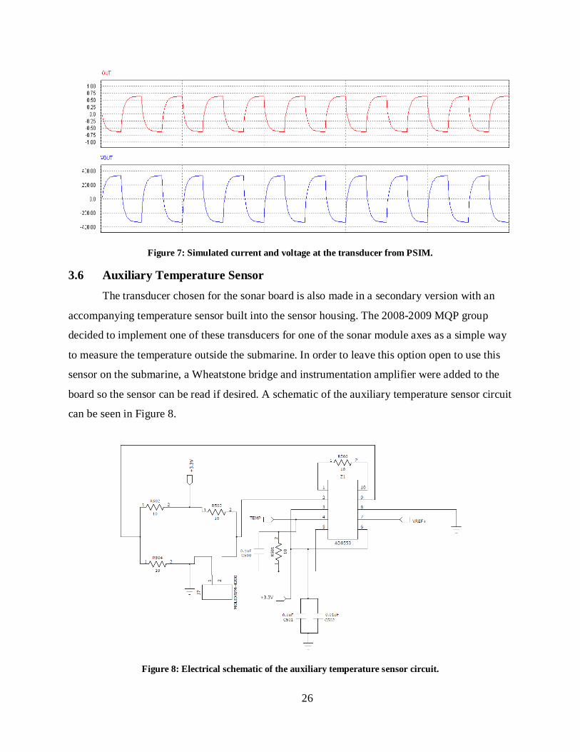
3.6 Auxiliary Temperature Sensor The transducer chosen for the sonar board is also made in a secondary version with an
accompanying temperature sensor built into the sensor housing. The 2008-2009 MQP group
decided to implement one of these transducers for one of the sonar module axes as a simple way
to measure the temperature outside the submarine. In order to leave this option open to use this
sensor on the submarine, a Wheatstone bridge and instrumentation amplifier were added to the
board so the sensor can be read if desired. A schematic of the auxiliary temperature sensor circuit
can be seen in Figure 8.
Figure 8: Electrical schematic of the auxiliary temperature sensor circuit.
27
The transducer with the temperature sensor has different electrical characteristics than the
transducer that is solely used for distance measured. While both operate at 200 kHz, they have
different equivalent resistances and capacitances. Section 3.5 describes how the different
properties of the sensors were accounted for when designing the board. Also, this transducer has
a different connector than the other two to accommodate the extra conductor for the temperature
sensor. The connector will need to be changed to fit the RCA connector on the sonar board.
3.7 Computer Circuit Design and Fabrication All of the electrical design for the board was performed using a software package
produced by Mentor Graphics called PADS. PADS is made of three separate modules which
were used during various stages of the design process. PADS Logic was used to create the
electrical schematics for the board. Once the schematics were mostly finalized, PADS Layout
was employed to simulate the layout of the physical components on the board. Several iterations
were performed during the layout process in order to find a layout which provided ease of
debugging and minimal space requirements. After the layout was completed, the final step in
design was to decide where the connections between each component would be placed. This step
was done using PADS Router. When all the traces had been placed, PADS was used to generate
Gerber files for manufacturing the PCBs. Before sending the files to the manufacturer, they were
processed by an automated online Design Rule Checking (DRC) system. This program processes
the files to ensure that the board can be physically manufactured as it is designed. Once the
circuit had passed through the DRC process, the files were submitted to Advanced Circuits to be
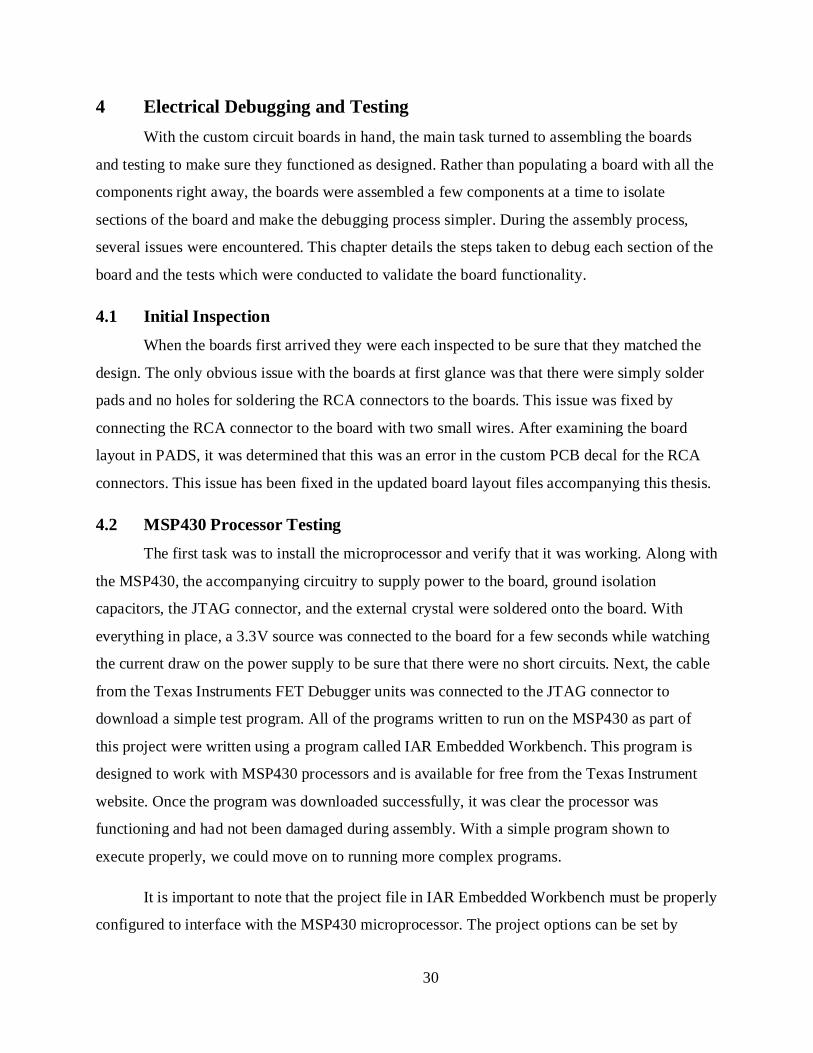
fabricated. The layout of the completed circuit board can be seen in Figure 9. The circuit boards
from Advanced Circuits, one of which can be seen in Figure 10, arrived about a week after they
were ordered. The complete schematics for the sonar board are in Appendix A – Electrical
Schematics.
28
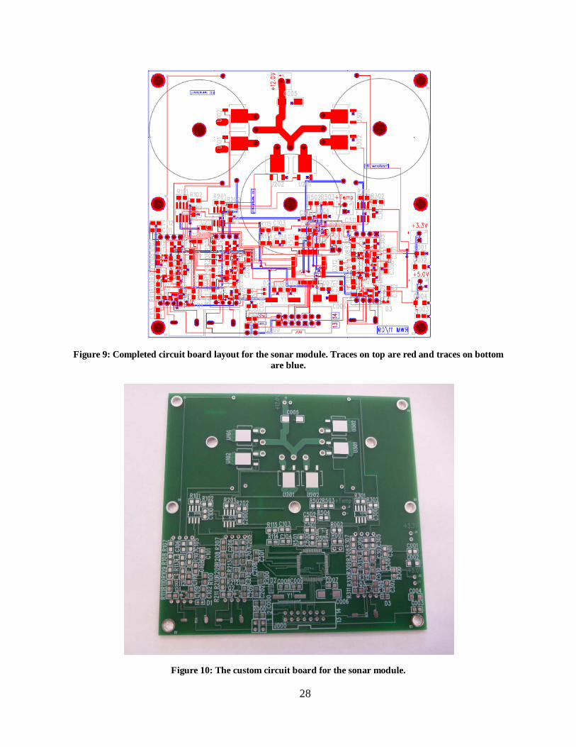
Figure 9: Completed circuit board layout for the sonar module. Traces on top are red and traces on bottom
are blue.
Figure 10: The custom circuit board for the sonar module.

29
3.8 Sonar Module Costs
One of the criteria for the sonar module was that it be inexpensive compared to other
commercially available alternatives. The largest cost for the module was the three transducers
which each cost $60.28. The custom circuit boards were $156.20 to purchase 4, but we were
given 1 free, for a total of 5. This gives an average cost per board of $31.24. The electrical
components for a single board cost $117.65. This cost includes the relays, custom transformers,
and necessary passive electronic components. The housing and mounting plate for the sonar,
discussed in Chapter 7, were both built with WPI’s rapid prototyping machine. The cost for the
materials for these parts was $31.20. If more than one module were to be produced at a time,
some of these costs would decrease significantly due to price breaks on the electronic
components and boards for larger quantities. Even built as a single prototype, the entire module
only cost $360.93, well below the design specified cost of $500.00. A detailed breakdown of the
cost for each component of the sonar module can be found in Appendix C - Sonar Module Cost
Breakdown.
.
30
4 Electrical Debugging and Testing With the custom circuit boards in hand, the main task turned to assembling the boards
and testing to make sure they functioned as designed. Rather than populating a board with all the
components right away, the boards were assembled a few components at a time to isolate
sections of the board and make the debugging process simpler. During the assembly process,
several issues were encountered. This chapter details the steps taken to debug each section of the
board and the tests which were conducted to validate the board functionality.
4.1 Initial Inspection When the boards first arrived they were each inspected to be sure that they matched the
design. The only obvious issue with the boards at first glance was that there were simply solder
pads and no holes for soldering the RCA connectors to the boards. This issue was fixed by
connecting the RCA connector to the board with two small wires. After examining the board
layout in PADS, it was determined that this was an error in the custom PCB decal for the RCA
connectors. This issue has been fixed in the updated board layout files accompanying this thesis.
4.2 MSP430 Processor Testing The first task was to install the microprocessor and verify that it was working. Along with
the MSP430, the accompanying circuitry to supply power to the board, ground isolation
capacitors, the JTAG connector, and the external crystal were soldered onto the board. With
everything in place, a 3.3V source was connected to the board for a few seconds while watching
the current draw on the power supply to be sure that there were no short circuits. Next, the cable
from the Texas Instruments FET Debugger units was connected to the JTAG connector to
download a simple test program. All of the programs written to run on the MSP430 as part of
this project were written using a program called IAR Embedded Workbench. This program is
designed to work with MSP430 processors and is available for free from the Texas Instrument
website. Once the program was downloaded successfully, it was clear the processor was
functioning and had not been damaged during assembly. With a simple program shown to
execute properly, we could move on to running more complex programs.
It is important to note that the project file in IAR Embedded Workbench must be properly
configured to interface with the MSP430 microprocessor. The project options can be set by
31
pressing the key sequence Alt-F7. The model number of the processor, in this case
MSP430F235, must be selected in the Device section on the Target tab of the General Options
Category. The Driver option on the Setup tab of the Debugger category needs to be changed
from Simulator to FET Debugger. Changing this option is critical. If the option is left with
Simulator selected, the code will compile and seem to download to the processor, but will only
run in a virtual machine on the PC.
4.3 Receive Circuit Testing After verifying that the processor was functioning properly, the next section of the circuit
that was tested was the receive circuitry. This was tested first because a function generator could
be temporarily substituted for the transmit portion of the circuit. The op-amps were soldered in
place and power was applied briefly to check for any short circuits. This was done one op-amp at
a time to isolate any problems with the individual op-amps. Only the op-amps for one of the
three axes were soldered in place for this initial testing. Once the testing was completed and all
the known problems with the receive circuitry were fixed, the remaining two axes were
populated and tested.
In Section 3.4, it is explained that the op-amps use a voltage reference supplied from the
MSP430 processor. By default, this voltage reference is turned off and connected to ground. The
two possible reference voltages generated are 1.5V and 2.5V, but the sonar module is designed
around the 2.5V reference. A short test program was written to set the appropriate registers in the
processor to turn on the voltage reference. When the program was downloaded to the chip and
run, a digital multi-meter was used to verify that the VREF+ pin on the MSP430 was outputting
2.5V. Because the voltage reference for the op-amps is 1.25V from the voltage divider, the
multi-meter was also used to check that voltage on pin 1 of all three op-amps was 1.25V. This
step was critical to the receive circuit because without a working voltage reference, only half the
signal could be measured.
4.4 Transformer Testing To supply the necessary power to the ultrasonic transducers, custom transformers were
designed and assembled as described in Section 3.5. Though the simulations showed that the
transformers would behave as designed, they were not purchased components, so they were
tested to validate their functionality before installing them in the transmit circuit. To test the
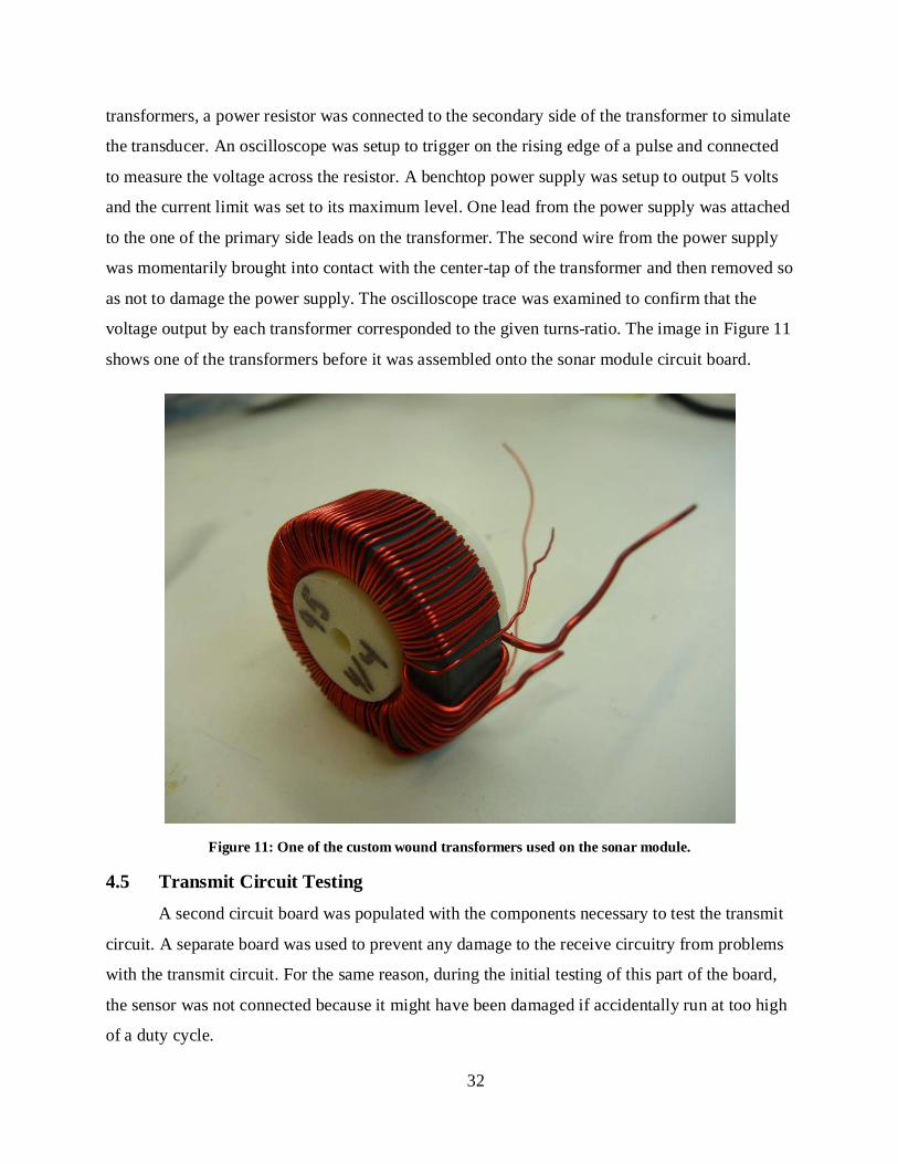
32
transformers, a power resistor was connected to the secondary side of the transformer to simulate
the transducer. An oscilloscope was setup to trigger on the rising edge of a pulse and connected
to measure the voltage across the resistor. A benchtop power supply was setup to output 5 volts
and the current limit was set to its maximum level. One lead from the power supply was attached
to the one of the primary side leads on the transformer. The second wire from the power supply
was momentarily brought into contact with the center-tap of the transformer and then removed so
as not to damage the power supply. The oscilloscope trace was examined to confirm that the
voltage output by each transformer corresponded to the given turns-ratio. The image in Figure 11
shows one of the transformers before it was assembled onto the sonar module circuit board.
Figure 11: One of the custom wound transformers used on the sonar module.
4.5 Transmit Circuit Testing A second circuit board was populated with the components necessary to test the transmit
circuit. A separate board was used to prevent any damage to the receive circuitry from problems
with the transmit circuit. For the same reason, during the initial testing of this part of the board,
the sensor was not connected because it might have been damaged if accidentally run at too high
of a duty cycle.
33
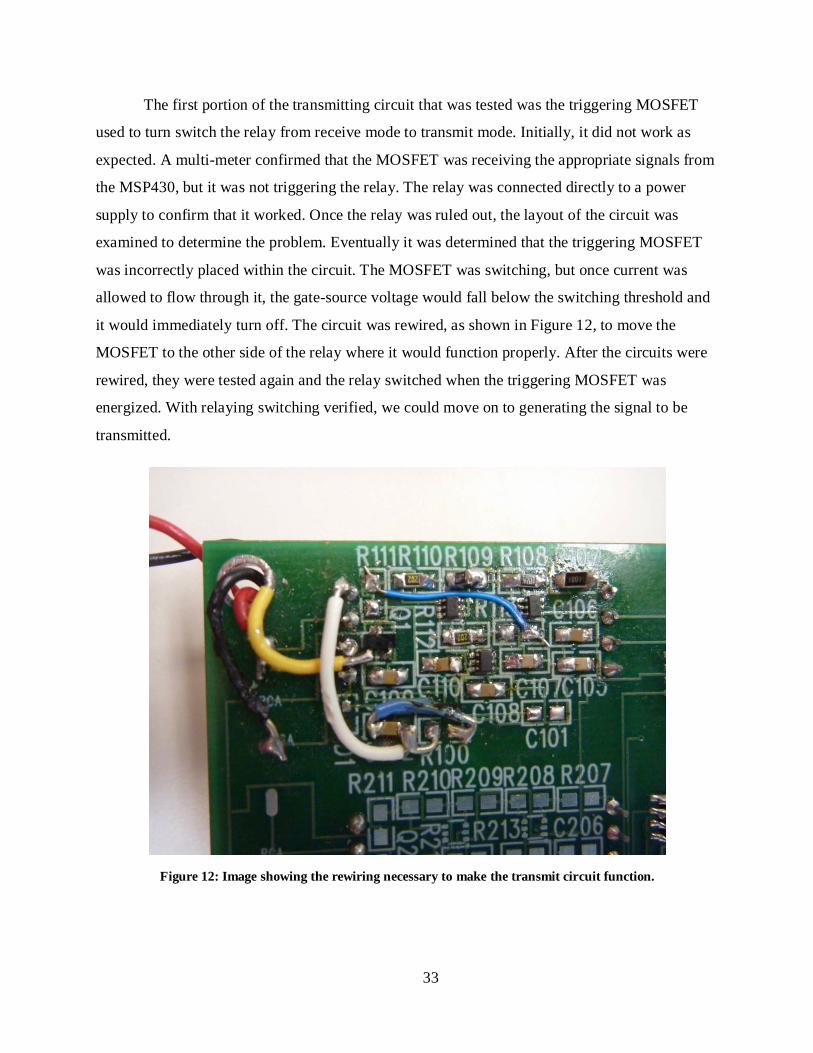
The first portion of the transmitting circuit that was tested was the triggering MOSFET
used to turn switch the relay from receive mode to transmit mode. Initially, it did not work as
expected. A multi-meter confirmed that the MOSFET was receiving the appropriate signals from
the MSP430, but it was not triggering the relay. The relay was connected directly to a power
supply to confirm that it worked. Once the relay was ruled out, the layout of the circuit was
examined to determine the problem. Eventually it was determined that the triggering MOSFET
was incorrectly placed within the circuit. The MOSFET was switching, but once current was
allowed to flow through it, the gate-source voltage would fall below the switching threshold and
it would immediately turn off. The circuit was rewired, as shown in Figure 12, to move the
MOSFET to the other side of the relay where it would function properly. After the circuits were
rewired, they were tested again and the relay switched when the triggering MOSFET was
energized. With relaying switching verified, we could move on to generating the signal to be
transmitted.
Figure 12: Image showing the rewiring necessary to make the transmit circuit function.
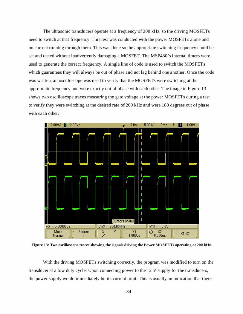
34
The ultrasonic transducers operate at a frequency of 200 kHz, so the driving MOSFETs
need to switch at that frequency. This test was conducted with the power MOSFETs alone and
no current running through them. This was done so the appropriate switching frequency could be
set and tested without inadvertently damaging a MOSFET. The MSP430’s internal timers were
used to generate the correct frequency. A single line of code is used to switch the MOSFETs
which guarantees they will always be out of phase and not lag behind one another. Once the code
was written, an oscilloscope was used to verify that the MOSFETs were switching at the
appropriate frequency and were exactly out of phase with each other. The image in Figure 13
shows two oscilloscope traces measuring the gate voltage at the power MOSFETs during a test
to verify they were switching at the desired rate of 200 kHz and were 180 degrees out of phase
with each other.
Figure 13: Two oscilloscope traces showing the signals driving the Power MOSFETs operating at 200 kHz.
With the driving MOSFETs switching correctly, the program was modified to turn on the
transducer at a low duty cycle. Upon connecting power to the 12 V supply for the transducers,
the power supply would immediately hit its current limit. This is usually an indication that there
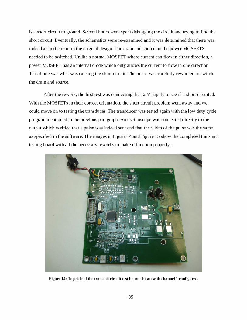
35
is a short circuit to ground. Several hours were spent debugging the circuit and trying to find the
short circuit. Eventually, the schematics were re-examined and it was determined that there was
indeed a short circuit in the original design. The drain and source on the power MOSFETS
needed to be switched. Unlike a normal MOSFET where current can flow in either direction, a
power MOSFET has an internal diode which only allows the current to flow in one direction.
This diode was what was causing the short circuit. The board was carefully reworked to switch
the drain and source.
After the rework, the first test was connecting the 12 V supply to see if it short circuited.
With the MOSFETs in their correct orientation, the short circuit problem went away and we
could move on to testing the transducer. The transducer was tested again with the low duty cycle
program mentioned in the previous paragraph. An oscilloscope was connected directly to the
output which verified that a pulse was indeed sent and that the width of the pulse was the same
as specified in the software. The images in Figure 14 and Figure 15 show the completed transmit
testing board with all the necessary reworks to make it function properly.
Figure 14: Top side of the transmit circuit test board shown with channel 1 configured.
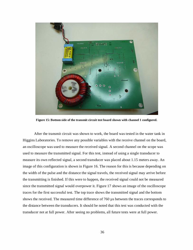
36
Figure 15: Bottom side of the transmit circuit test board shown with channel 1 configured.
After the transmit circuit was shown to work, the board was tested in the water tank in
Higgins Laboratories. To remove any possible variables with the receive channel on the board,
an oscilloscope was used to measure the received signal. A second channel on the scope was
used to measure the transmitted signal. For this test, instead of using a single transducer to
measure its own reflected signal, a second transducer was placed about 1.15 meters away. An
image of this configuration is shown in Figure 16. The reason for this is because depending on
the width of the pulse and the distance the signal travels, the received signal may arrive before
the transmitting is finished. If this were to happen, the received signal could not be measured
since the transmitted signal would overpower it. Figure 17 shows an image of the oscilloscope
traces for the first successful test. The top trace shows the transmitted signal and the bottom
shows the received. The measured time difference of 760 µs between the traces corresponds to
the distance between the transducers. It should be noted that this test was conducted with the
transducer not at full power. After seeing no problems, all future tests were at full power.
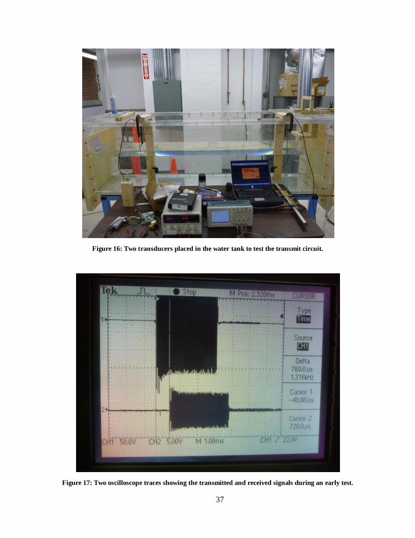
37
Figure 16: Two transducers placed in the water tank to test the transmit circuit.
Figure 17: Two oscilloscope traces showing the transmitted and received signals during an early test.
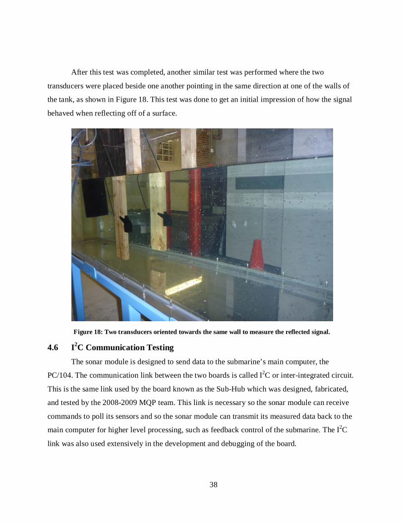
38
After this test was completed, another similar test was performed where the two
transducers were placed beside one another pointing in the same direction at one of the walls of
the tank, as shown in Figure 18. This test was done to get an initial impression of how the signal
behaved when reflecting off of a surface.
Figure 18: Two transducers oriented towards the same wall to measure the reflected signal.
4.6 I2C Communication Testing The sonar module is designed to send data to the submarine’s main computer, the
PC/104. The communication link between the two boards is called I2C or inter-integrated circuit.
This is the same link used by the board known as the Sub-Hub which was designed, fabricated,
and tested by the 2008-2009 MQP team. This link is necessary so the sonar module can receive
commands to poll its sensors and so the sonar module can transmit its measured data back to the
main computer for higher level processing, such as feedback control of the submarine. The I2C
link was also used extensively in the development and debugging of the board.
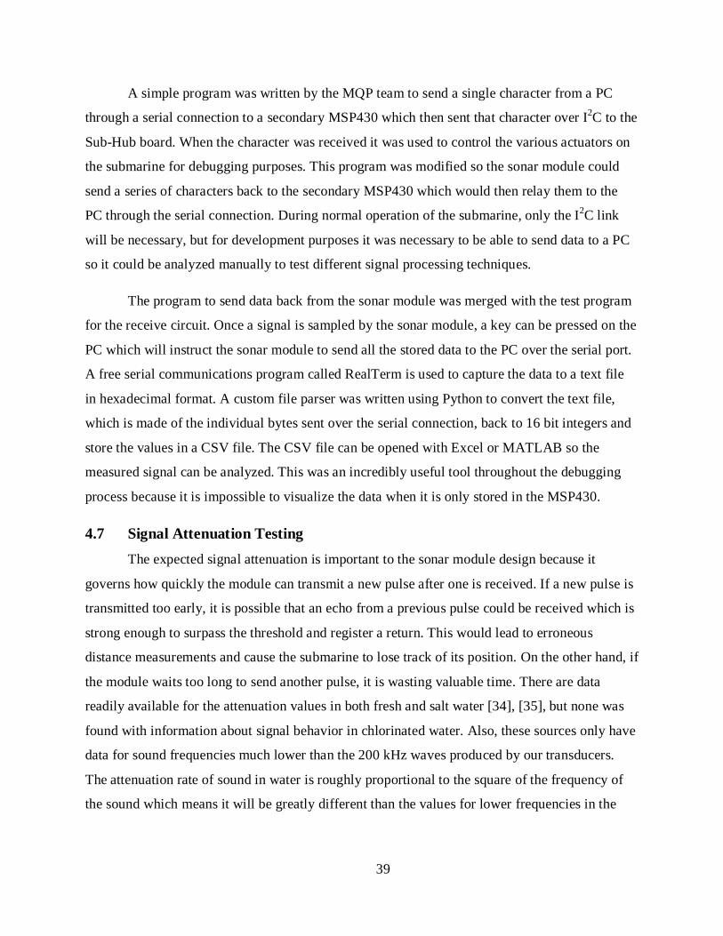
39
A simple program was written by the MQP team to send a single character from a PC
through a serial connection to a secondary MSP430 which then sent that character over I2C to the
Sub-Hub board. When the character was received it was used to control the various actuators on
the submarine for debugging purposes. This program was modified so the sonar module could
send a series of characters back to the secondary MSP430 which would then relay them to the
PC through the serial connection. During normal operation of the submarine, only the I2C link
will be necessary, but for development purposes it was necessary to be able to send data to a PC
so it could be analyzed manually to test different signal processing techniques.
The program to send data back from the sonar module was merged with the test program
for the receive circuit. Once a signal is sampled by the sonar module, a key can be pressed on the
PC which will instruct the sonar module to send all the stored data to the PC over the serial port.
A free serial communications program called RealTerm is used to capture the data to a text file
in hexadecimal format. A custom file parser was written using Python to convert the text file,
which is made of the individual bytes sent over the serial connection, back to 16 bit integers and
store the values in a CSV file. The CSV file can be opened with Excel or MATLAB so the
measured signal can be analyzed. This was an incredibly useful tool throughout the debugging
process because it is impossible to visualize the data when it is only stored in the MSP430.
4.7 Signal Attenuation Testing The expected signal attenuation is important to the sonar module design because it
governs how quickly the module can transmit a new pulse after one is received. If a new pulse is
transmitted too early, it is possible that an echo from a previous pulse could be received which is
strong enough to surpass the threshold and register a return. This would lead to erroneous
distance measurements and cause the submarine to lose track of its position. On the other hand, if
the module waits too long to send another pulse, it is wasting valuable time. There are data
readily available for the attenuation values in both fresh and salt water [34], [35], but none was
found with information about signal behavior in chlorinated water. Also, these sources only have
data for sound frequencies much lower than the 200 kHz waves produced by our transducers.
The attenuation rate of sound in water is roughly proportional to the square of the frequency of
the sound which means it will be greatly different than the values for lower frequencies in the
40
literature [36]. Since the sonar module will be operating in a chlorinated environment and at a
higher frequency, the attenuation rate for the transmitted sound was determined experimentally.
An experiment was conducted to determine the attenuation of the transmitted sonar signal
in the pool water. Two transducers were used for this test, with one connected to a board setup to
transmit a single pulse and the other connected only to the oscilloscope. A second channel on the
oscilloscope was connected to the transmitting transducer and the oscilloscope was configured to
trigger when the pulse was transmitted so it could capture both the transmitted and received
pulses. An oscilloscope was used instead of the receive channel on the sonar module because it
can capture the peak voltage signal whereas the sonar module would modify the received voltage
with the op-amps. Were the receive channel used instead, the peak voltages could be above the
maximum value of the ADC and we would not be able to determine by how much the signal had
attenuated.
The transducers were placed underwater near the edge of the pool at a set distance apart
from each other. With the oscilloscope ready to capture a pulse, the IAR Embedded Workbench
was used to start the transmitting board and send the pulse. An image was taken of the captured
signal on the oscilloscope and the corresponding image number and oscilloscope settings were
recorded. This process was repeated over a range of several meters at 50 centimeter intervals.
One data point is missing because a support column next to the pool obstructed the structure
holding the sensor.
Each image was manually analyzed to determine the average received voltage. These
voltages were then used to calculate the received power given the known resistance of the
transducer. The received and transmitted powers were compared and converted to decibels. The
measurements from the experiment are shown plotted in Figure 19 below.
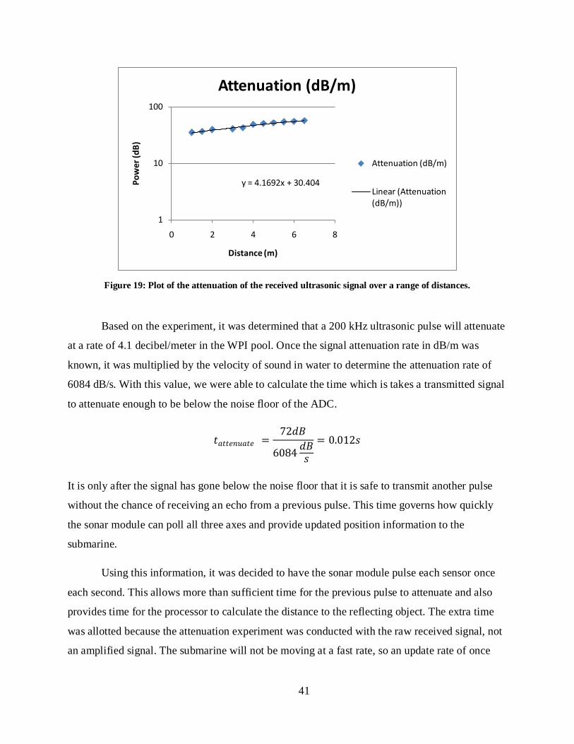
41
Figure 19: Plot of the attenuation of the received ultrasonic signal over a range of distances.
Based on the experiment, it was determined that a 200 kHz ultrasonic pulse will attenuate
at a rate of 4.1 decibel/meter in the WPI pool. Once the signal attenuation rate in dB/m was
known, it was multiplied by the velocity of sound in water to determine the attenuation rate of
6084 dB/s. With this value, we were able to calculate the time which is takes a transmitted signal
to attenuate enough to be below the noise floor of the ADC.
𝐼𝐼𝑊𝑊𝐼𝐼𝐼𝐼𝐼𝐼𝐼𝐼𝑇𝑇𝑊𝑊𝐼𝐼𝐼𝐼 =72𝑑𝑑𝑑𝑑
6084 𝑑𝑑𝑑𝑑𝐼𝐼= 0.012𝐼𝐼
It is only after the signal has gone below the noise floor that it is safe to transmit another pulse
without the chance of receiving an echo from a previous pulse. This time governs how quickly
the sonar module can poll all three axes and provide updated position information to the
submarine.
Using this information, it was decided to have the sonar module pulse each sensor once
each second. This allows more than sufficient time for the previous pulse to attenuate and also
provides time for the processor to calculate the distance to the reflecting object. The extra time
was allotted because the attenuation experiment was conducted with the raw received signal, not
an amplified signal. The submarine will not be moving at a fast rate, so an update rate of once
y = 4.1692x + 30.404
1
10
100
0 2 4 6 8
Pow
er (d
B)
Distance (m)
Attenuation (dB/m)
Attenuation (dB/m)
Linear (Attenuation (dB/m))
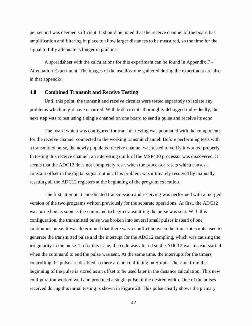
42
per second was deemed sufficient. It should be noted that the receive channel of the board has
amplification and filtering in place to allow larger distances to be measured, so the time for the
signal to fully attenuate is longer in practice.
A spreadsheet with the calculations for this experiment can be found in Appendix F –
Attenuation Experiment. The images of the oscilloscope gathered during the experiment are also
in that appendix.
4.8 Combined Transmit and Receive Testing Until this point, the transmit and receive circuits were tested separately to isolate any
problems which might have occurred. With both circuits thoroughly debugged individually, the
next step was to test using a single channel on one board to send a pulse and receive its echo.
The board which was configured for transmit testing was populated with the components
for the receive channel connected to the working transmit channel. Before performing tests with
a transmitted pulse, the newly populated receive channel was tested to verify it worked properly.
In testing this receive channel, an interesting quirk of the MSP430 processor was discovered. It
seems that the ADC12 does not completely reset when the processor resets which causes a
constant offset in the digital signal output. This problem was ultimately resolved by manually
resetting all the ADC12 registers at the beginning of the program execution.
The first attempt at coordinated transmission and receiving was performed with a merged
version of the two programs written previously for the separate operations. At first, the ADC12
was turned on as soon as the command to begin transmitting the pulse was sent. With this
configuration, the transmitted pulse was broken into several small pulses instead of one
continuous pulse. It was determined that there was a conflict between the timer interrupts used to
generate the transmitted pulse and the interrupt for the ADC12 sampling, which was causing the
irregularity in the pulse. To fix this issue, the code was altered so the ADC12 was instead started
when the command to end the pulse was sent. At the same time, the interrupts for the timers
controlling the pulse are disabled so there are no conflicting interrupts. The time from the
beginning of the pulse is stored as an offset to be used later in the distance calculation. This new
configuration worked well and produced a single pulse of the desired width. One of the pulses
received during this initial testing is shown in Figure 20. This pulse clearly shows the primary
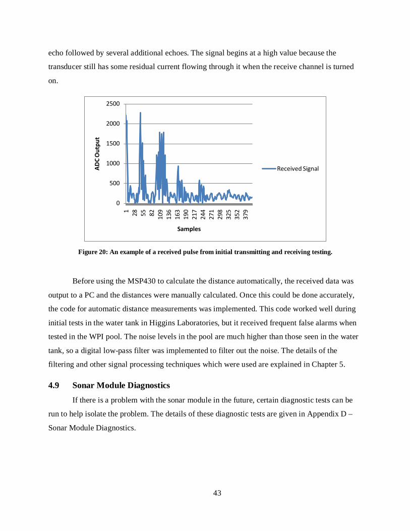
43
echo followed by several additional echoes. The signal begins at a high value because the
transducer still has some residual current flowing through it when the receive channel is turned
on.
Figure 20: An example of a received pulse from initial transmitting and receiving testing.
Before using the MSP430 to calculate the distance automatically, the received data was
output to a PC and the distances were manually calculated. Once this could be done accurately,
the code for automatic distance measurements was implemented. This code worked well during
initial tests in the water tank in Higgins Laboratories, but it received frequent false alarms when
tested in the WPI pool. The noise levels in the pool are much higher than those seen in the water
tank, so a digital low-pass filter was implemented to filter out the noise. The details of the
filtering and other signal processing techniques which were used are explained in Chapter 5.
4.9 Sonar Module Diagnostics
If there is a problem with the sonar module in the future, certain diagnostic tests can be
run to help isolate the problem. The details of these diagnostic tests are given in Appendix D –
Sonar Module Diagnostics.
0
500
1000
1500
2000
2500
1 28 55 82 109
136
163
190
217
244
271
298
325
352
379
AD
C O
utpu
t
Samples
Received Signal
44
5 Received Signal Processing When one of the submarine’s transducers receives an echoed signal after a transmission,
the signal must be processed. The signal processing is necessary for two primary reasons:
determining the strength of the signal and calculating the time-of-flight. Firstly, the processor
must decide if the signal is strong enough to be classified as a primary echo and not a secondary
echo or other noise. The solid walls of the tank act as acoustic mirrors, allowing the transmitted
sound to be reflected several times before it attenuates. It is possible that the sensor could receive
one of these secondary echoes which, if mistaken for a primary echo, could lead to an incorrect
distance measurement and ultimately an incorrect localization calculation. Also, because the tank
is an inherently noisy acoustic environment due to the filtration system and other machinery in
the area, the signal processor needs to be able to distinguish the echoes of its transmitted signals
from other environmental disturbances.
The second reason for signal processing is to determine the time the signal took to travel
to the reflecting surface and return to the sensor. This time is commonly referred to as the time –
of-flight or TOF. Using the TOF and the speed of sound in water, the sonar module can calculate
the distance to the object which reflected the signal. The distances measured on the three axes of
the module are transmitted back to the PC/104 where the location of the submarine can be
calculated.
This chapter explains in detail the electronic and software based methods used to
condition and process the signal to ultimately calculate the distance measurement required. First,
the electronic amplification and filtering will be discussed. Once the signal has undergone these
processes, it is converted to a digital signal which can then be analyzed by the microprocessor.
The received digital signal is further processed to decide if the signal is useful and to calculate
the distance if so.
5.1 Hardware Signal Processing It is important to perform some hardware signal processing before a signal is fed into the
processor for a number of reasons. If the received signal is sufficiently attenuated, it may not
produce a large enough voltage to be read by the MSP430’s analog to digital convertor. Since the
returned signal could be weak, it is possible that it could fall below the noise level of the tank
45
and blend in with the background sounds. Hardware based filters can be used to remove certain
frequencies of noise which will lead to a cleaner signal for the MSP430 to process. The hardware
processing methods used here have the benefit of working in real time whereas the software
based processing are discrete and limited by the speed of the ADC and the MSP430’s processor.
5.1.1 Amplification
Based on the experimental data from Chapter 3, we know that the 200 kHz ultrasonic
signal attenuates at a rate of 4.1 dB/meter in the chlorinated water. This means there will be a
large deviation in the strength of a signal reflected at close range and one reflected from a
surface on the far side of the pool. Signals which have traveled a relatively long distance might
have attenuated enough to make them difficult to distinguish from the background noise.
To account for the reduction in signal strength, the incoming signal is amplified to bring
the desired signal out of the noise. It is important to note that the noise is amplified too, so the
gain for amplification should not be chosen arbitrarily. Two inverting operational amplifiers are
used in series to increase the voltage of the received signal. The amplification will likely cause
the sensor to saturate at short range because the op-amps will try to amplify a voltage outside of
their output range. There is no danger of over-amplifying in this scenario because we are only
concerned with the time that the signal amplitude reaches a given threshold and not by how
much it surpasses that threshold. If the sensor becomes saturated from a short range reflection
because of the gain, this will not have any effect on the distance measurement.
The two op-amps built into the receive circuit are configured as inverting op-amps. This
means that a positive voltage input gives a negative voltage output and vice versa. However, the
op-amps themselves can only output voltages between 0.0V and 3.3V. This means that a positive
input voltage into the first op-amp would be amplified to 0.0V because of the negative gain.
Likewise, a negative voltage input would survive the first op-amp, being amplified to a positive
voltage, but would be lost going through the second amplifier. To stop this problem from
occurring, the op-amps use a reference voltage generated by a voltage divider to offset the
signals to the middle of the band which can be read by the ADC. The voltage divider reference is
designed to nominally be 1.25V. With this voltage reference, both positive and negative input
voltages can be amplified without automatically hitting the upper or lower rail of the sensor.
46
Both op-amps are AC coupled with a capacitor in series with the input resistor. The AC
coupling means that only AC signals will pass through since any DC signal will be blocked by
the capacitor. Without the AC coupling, the second op-amp would amplify both the received
signal and the 1.25V reference, causing it to saturate constantly. The AC coupling ensures that
only the received signal is amplified.
5.1.1.1 Op-Amp Gains
The original design of the receive circuit by the MQP group called for a total gain of 324
(-18 twice) through the op-amps using 2 kΩ and 36 kΩ resistors. These values were chosen as
placeholders to be replaced with other resistors once the characteristics of the background noise
and sound attenuation were better known. After basic noise measurements were conducted in the
pool, it was determined that this was much more gain than was needed. The gain of 324 was, in
fact, too much because it raised the level of noise high enough were discerning a pulse within the
noise was difficult. The gain was changed to a total gain of 10 with a gain of -5 for the first op-
amp and -2 for the second. This value provides sufficient gain to measure signals at the furthest
distances that will be measured while keeping the noise level at much lower amplitude.
5.1.2 Analog to Digital Conversion
Once the received signal has been amplified, it must be converted from its continuous
analog form to a discrete digital signal which can in turn be processed by the software on the
MSP430. The model of MSP430 used for this sonar module has two analog to digital convertors,
ADC10 and ADC12, which have 10 and 12-bits of resolution respectively. The ADC12 was
chosen for the sonar measurements to take advantage of the extra resolution it offers. Being a 12-
bit ADC, the ADC12 outputs a digital value from 0 to 4095, depending on the amplitude of the
input signal between 0.0V and 2.5V. The hardware is capable of sampling at a rate of up to
200,000 samples per second. The following is the formula which is used to perform the
conversion.
𝑁𝑁𝐴𝐴𝐴𝐴𝐴𝐴 = 4095 ∗𝑉𝑉𝐼𝐼𝑁𝑁 − 𝑉𝑉𝑅𝑅−𝑉𝑉𝑅𝑅+ − 𝑉𝑉𝑅𝑅−
47
It has internal voltage references, 𝑉𝑉𝑅𝑅+ and 𝑉𝑉𝑅𝑅− in the formula above, which can be set
programmatically to adjust the range of voltages accepted for conversion. The sonar module is
configured to use a range from 0.0V to 2.5V for input to the ADC [37].
5.1.2.1 Nyquist-Shannon Sampling Rate
In signal processing, the Nyquist-Shannon Sampling Theorem is commonly used to
determine how often a signal must be sampled so that none of the information is lost in the
analog to digital conversion. The Nyquist-Shannon Sampling Theorem states:
“If a function contains no frequencies higher than W, it is completely determined by giving its
ordinates at a series of points spaced 1/2 W seconds apart [38].”
This is another way of stating that the rate at which a signal is sampled must be at least twice the
maximum frequency of the signal being measured to fully reconstruct the signal from the
measurements. This is known as the Nyquist-Shannon Sampling Rate. As a consequence of this
phenomenon, an ADC can only fully reconstruct signals with frequencies which are less than
half of the ADC sampling rate.
The maximum sampling rate of the ADC12 on the MSP430 is around 200,000 samples
per second and the pulses transmitted by the transducers are at 200 kHz. Were it necessary to
completely reconstruct the received signal, this would present a problem and the ADC would
probably have to be replaced with a faster version. However, the received signal measured by the
sonar module is not communicating any data in the pulse itself, but only in the time it arrives at
the sensor. The envelope of the signal is sufficient to determine the time of arrival, and for this
reason, the module does not need to satisfy the Nyquist-Shannon sampling rate.
5.1.2.2 Sub-Nyquist-Shannon Rate Sampling
The maximum rate at which the MSP430’s 12 bit ADC can convert a signal is around
200 kHz. With the output center frequency of the transducers at 200 kHz, there is no way this
hardware configuration can satisfy the Nyquist-Shannon Rate and completely reconstruct the
signal. Were the sonar module intended to transmit encoded data through its pulses, this might
pose a problem; however, the module does not need to reconstruct the signal and is primarily
concerned with its relative strength. The only information which is critical in the case of the
sonar module is the time-of-flight of the signal. Sub-sampling has no effect on the speed of the
48
signal, so the time-of-flight will not be changed. Therefore, the signal can be sampled at a lower
rate than the Nyquist-Shannon rate and still produce the necessary information.
A consequence of sampling a signal at a lower frequency than its constitutive
components is that the high frequency components above the sampling rate are folded down onto
the lower frequency signals with the sampling rate acting as a pivot point. This is known as
signal aliasing because a higher frequency signal appears as if it were a lower frequency. The
signal aliasing effect is exploited to alias the 200 kHz signal from the transducer to a much lower
frequency which can be detected by the ADC12. The sampling frequency was chosen so that the
aliased version of the signal appears in a section of the spectrum which yields a high signal to
noise ratio.
5.1.2.2.1 Measuring the Sampling Rate of the ADC12
The documentation for the MSP430 gives information about the maximum conversion
rate of the ADC, but this rate can only be achieved under optimal conditions with minimal
processing between samples. The formula given in the documentation for calculating the total
time to capture and convert a sample is the following:
𝐼𝐼 = 𝐼𝐼𝐼𝐼𝑠𝑠𝐼𝐼𝐼𝐼 + 𝐼𝐼𝐼𝐼𝑊𝑊𝐼𝐼𝑎𝑎𝑉𝑉𝐼𝐼 + 𝐼𝐼𝐼𝐼𝑉𝑉𝐼𝐼𝑐𝑐𝐼𝐼𝐼𝐼𝐼𝐼
𝐼𝐼𝐼𝐼𝑊𝑊𝐼𝐼𝑎𝑎𝑉𝑉𝐼𝐼 = 𝑆𝑆𝑆𝑆𝑇𝑇0 ∗ 𝐴𝐴𝐴𝐴𝐴𝐴12𝐴𝐴𝐶𝐶𝐶𝐶
𝐼𝐼𝐼𝐼𝑉𝑉𝐼𝐼𝑐𝑐𝐼𝐼𝐼𝐼𝐼𝐼 = 13 ∗ 𝐴𝐴𝐴𝐴𝐴𝐴12𝐴𝐴𝐶𝐶𝐶𝐶
The synchronization time is a small fixed time which depends on the exact model of the
processor and varies within a range of values depending on the batch of processors. The sample
time is the amount of time during which the ADC is gathering data. In the case of the sonar
module, we do not want to sample at the maximum rate, so we use the available ADC registers to
adjust it. The sampling time can be changed using either the SHT0 (sample hold time) register or
by changing the speed of the ADC’s clock reference ADC12CLK. The conversion time is fixed
at 13 clock cycles and can be adjusted by changing the speed of ADC12CLK [37].
Since the actual value of the synchronization time is unknown, the exact sampling rate
cannot be determined by the above formula. Instead, a few lines of code are added to an ADC
sampling program to measure the sample rate of the ADC directly using the on-board timers.
Before the ADC is configured, the onboard Timer A is setup without any interrupts enabled. This
49
turns on the register TAR which begins counting between 0 and 65535 continuously. Each time
the ADC triggers an interrupt the sample is read and processed as normal. The final line of code
where the process sample output is replaced with a statement to store the value of the TAR
register instead.
Once a sequence of data is gathered, it is transferred to a PC for analysis. When the data
is plotted, it produces a constant slope line or a saw-tooth pattern if TAR returned to zero during
sampling. The slope of the line is the number of processor cycles between each successive
sample of the ADC. Using this value and the software selectable speed of the ADC12CLK, the
sampling rate of the ADC can be determined with much greater certainty than the supplied
equation. This same method was also used to measure the execution time of different interrupt
service routines to make sure they had enough time to process before another interrupt triggered.
5.1.2.2.2 Determining the Ideal Sampling Rate for the ADC12
With the sampling rate of the ADC12 easily measured using software, the next step was
to determine the ideal sampling rate. Since the signal we desire to measure is being aliased onto a
lower frequency band, it is important to make that aliased frequency one which is not prevalent
within the background noise in the test environment. If the signal were aliased to a frequency
similar to a source of noise, it would increase the likelihood of a false reading because of the
decreased signal to noise ratio. One of the major limiting factors for the ADC sampling rate is
the amount of time needed for processing the received signal each time the interrupt triggers.
5.2 Software Signal Processing The analog to digital convertor samples the received signal and stores the values in the
ADC memory registers. Each time the sampling occurs, an interrupt is triggered so the value can
be moved to another location. The data is stored in the MSP430’s RAM because writing to the
flash memory would take too long. Once stored in RAM, the data is processed to determine if an
echo has been received.
5.2.1 Digital Low-Pass Filtering
The data output by the ADC12 is a mixture of environmental noise, electronics noise, and
the desired signal. One method of removing the high frequency noise from the data is to use a
digital low-pass filter. Like the name implies, a low-pass filter allows frequencies below a certain
50
value to pass and attenuates frequencies above that value. This is particularly useful with the
sonar module because we are using signal aliasing to our advantage and can decide where our
signal will fall in the spectrum. By choosing an appropriate sampling rate, the received signal
was made to appear in the low frequency end of the received spectrum. A cutoff frequency was
then chosen to remove the noise above the desired signal.
There are a number of types of digital filters available, but a finite impulse response, FIR,
low-pass filter was chosen for this application. Unlike an infinite impulse response, IIR, the FIR
has the advantage of always having a stable response, a fixed output delay, and fixed set of
coefficients for a given filter behavior [39], [40]. The equation which describes an FIR filter is
given as the following.
𝑠𝑠(𝐼𝐼) = 𝑏𝑏(𝑘𝑘)𝑥𝑥(𝐼𝐼 − 𝑘𝑘)𝑀𝑀−1
𝑘𝑘=0
In this equation, the output signal 𝑠𝑠(𝐼𝐼) is a summation of a series of M delayed inputs multiplied
by the filter coefficients. The delayed inputs are stored in a circular buffer where the newest
input constantly replaces the oldest input in the buffer. As the number of coefficients increases,
the output of the filter approaches the behavior of an ideal filter. The increased filter performance
comes at the cost of the additional computing time necessary to compute the additional multiply
and sum operations [39], [40].
5.2.1.1 Determining FIR Filter Coefficients
The processing time for the FIR filter is incredibly important because all the necessary
calculations need to be performed before the next ADC interrupt triggers. After some
experimentation using MATLAB, it was determined that 7 coefficients would be sufficient to
produce the desired filtering. To further increase the efficiency of the filter, an 8th coefficient
with a value of 0 was added so bitwise operations could be used to implement the circular buffer
instead of the more time intensive modulus division operation.
The coefficients of the filter are determined by first computing the value of the following
function for all 𝐼𝐼.
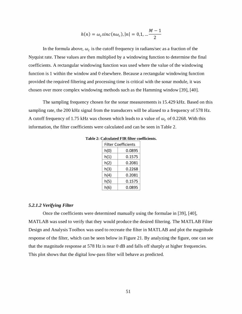
51
ℎ(𝐼𝐼) = 𝜔𝜔𝐼𝐼𝐼𝐼𝑟𝑟𝐼𝐼𝐼𝐼(𝐼𝐼𝜔𝜔𝐼𝐼), |𝐼𝐼| = 0,1, …𝑀𝑀 − 1
2
In the formula above, 𝜔𝜔𝐼𝐼 is the cutoff frequency in radians/sec as a fraction of the
Nyquist rate. These values are then multiplied by a windowing function to determine the final
coefficients. A rectangular windowing function was used where the value of the windowing
function is 1 within the window and 0 elsewhere. Because a rectangular windowing function
provided the required filtering and processing time is critical with the sonar module, it was
chosen over more complex windowing methods such as the Hamming window [39], [40].
The sampling frequency chosen for the sonar measurements is 15.429 kHz. Based on this
sampling rate, the 200 kHz signal from the transducers will be aliased to a frequency of 578 Hz.
A cutoff frequency of 1.75 kHz was chosen which leads to a value of 𝜔𝜔𝐼𝐼 of 0.2268. With this
information, the filter coefficients were calculated and can be seen in Table 2.
Table 2: Calculated FIR filter coefficients. Filter Coefficients h(0) 0.0895 h(1) 0.1575 h(2) 0.2081 h(3) 0.2268 h(4) 0.2081 h(5) 0.1575 h(6) 0.0895
5.2.1.2 Verifying Filter
Once the coefficients were determined manually using the formulae in [39], [40],
MATLAB was used to verify that they would produce the desired filtering. The MATLAB Filter
Design and Analysis Toolbox was used to recreate the filter in MATLAB and plot the magnitude
response of the filter, which can be seen below in Figure 21. By analyzing the figure, one can see
that the magnitude response at 578 Hz is near 0 dB and falls off sharply at higher frequencies.
This plot shows that the digital low-pass filter will behave as predicted.
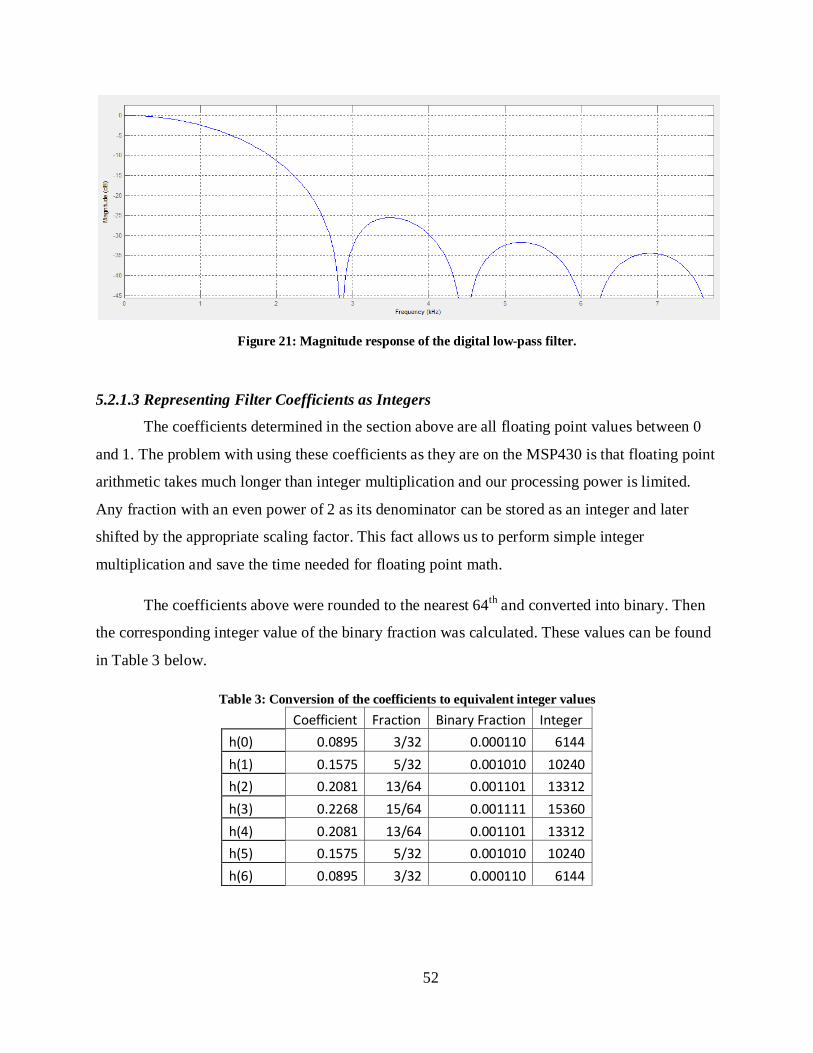
52
Figure 21: Magnitude response of the digital low-pass filter.
5.2.1.3 Representing Filter Coefficients as Integers
The coefficients determined in the section above are all floating point values between 0
and 1. The problem with using these coefficients as they are on the MSP430 is that floating point
arithmetic takes much longer than integer multiplication and our processing power is limited.
Any fraction with an even power of 2 as its denominator can be stored as an integer and later
shifted by the appropriate scaling factor. This fact allows us to perform simple integer
multiplication and save the time needed for floating point math.
The coefficients above were rounded to the nearest 64th and converted into binary. Then
the corresponding integer value of the binary fraction was calculated. These values can be found
in Table 3 below.
Table 3: Conversion of the coefficients to equivalent integer values
Coefficient Fraction Binary Fraction Integer
h(0) 0.0895 3/32 0.000110 6144 h(1) 0.1575 5/32 0.001010 10240 h(2) 0.2081 13/64 0.001101 13312 h(3) 0.2268 15/64 0.001111 15360 h(4) 0.2081 13/64 0.001101 13312 h(5) 0.1575 5/32 0.001010 10240 h(6) 0.0895 3/32 0.000110 6144
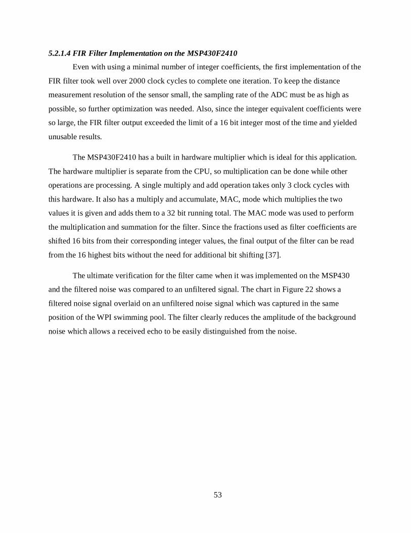
53
5.2.1.4 FIR Filter Implementation on the MSP430F2410
Even with using a minimal number of integer coefficients, the first implementation of the
FIR filter took well over 2000 clock cycles to complete one iteration. To keep the distance
measurement resolution of the sensor small, the sampling rate of the ADC must be as high as
possible, so further optimization was needed. Also, since the integer equivalent coefficients were
so large, the FIR filter output exceeded the limit of a 16 bit integer most of the time and yielded
unusable results.
The MSP430F2410 has a built in hardware multiplier which is ideal for this application.
The hardware multiplier is separate from the CPU, so multiplication can be done while other
operations are processing. A single multiply and add operation takes only 3 clock cycles with
this hardware. It also has a multiply and accumulate, MAC, mode which multiplies the two
values it is given and adds them to a 32 bit running total. The MAC mode was used to perform
the multiplication and summation for the filter. Since the fractions used as filter coefficients are
shifted 16 bits from their corresponding integer values, the final output of the filter can be read
from the 16 highest bits without the need for additional bit shifting [37].
The ultimate verification for the filter came when it was implemented on the MSP430
and the filtered noise was compared to an unfiltered signal. The chart in Figure 22 shows a
filtered noise signal overlaid on an unfiltered noise signal which was captured in the same
position of the WPI swimming pool. The filter clearly reduces the amplitude of the background
noise which allows a received echo to be easily distinguished from the noise.
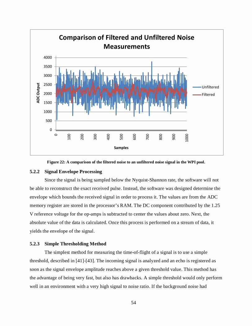
54
Figure 22: A comparison of the filtered noise to an unfiltered noise signal in the WPI pool.
5.2.2 Signal Envelope Processing
Since the signal is being sampled below the Nyquist-Shannon rate, the software will not
be able to reconstruct the exact received pulse. Instead, the software was designed determine the
envelope which bounds the received signal in order to process it. The values are from the ADC
memory register are stored in the processor’s RAM. The DC component contributed by the 1.25
V reference voltage for the op-amps is subtracted to center the values about zero. Next, the
absolute value of the data is calculated. Once this process is performed on a stream of data, it
yields the envelope of the signal.
5.2.3 Simple Thresholding Method
The simplest method for measuring the time-of-flight of a signal is to use a simple
threshold, described in [41]-[43]. The incoming signal is analyzed and an echo is registered as
soon as the signal envelope amplitude reaches above a given threshold value. This method has
the advantage of being very fast, but also has drawbacks. A simple threshold would only perform
well in an environment with a very high signal to noise ratio. If the background noise had
0
500
1000
1500
2000
2500
3000
3500
40000
100
200
300
400
500
600
700
800
900
1000
AD
C O
utpu
t
Samples
Comparison of Filtered and Unfiltered Noise Measurements
Unfiltered
Filtered
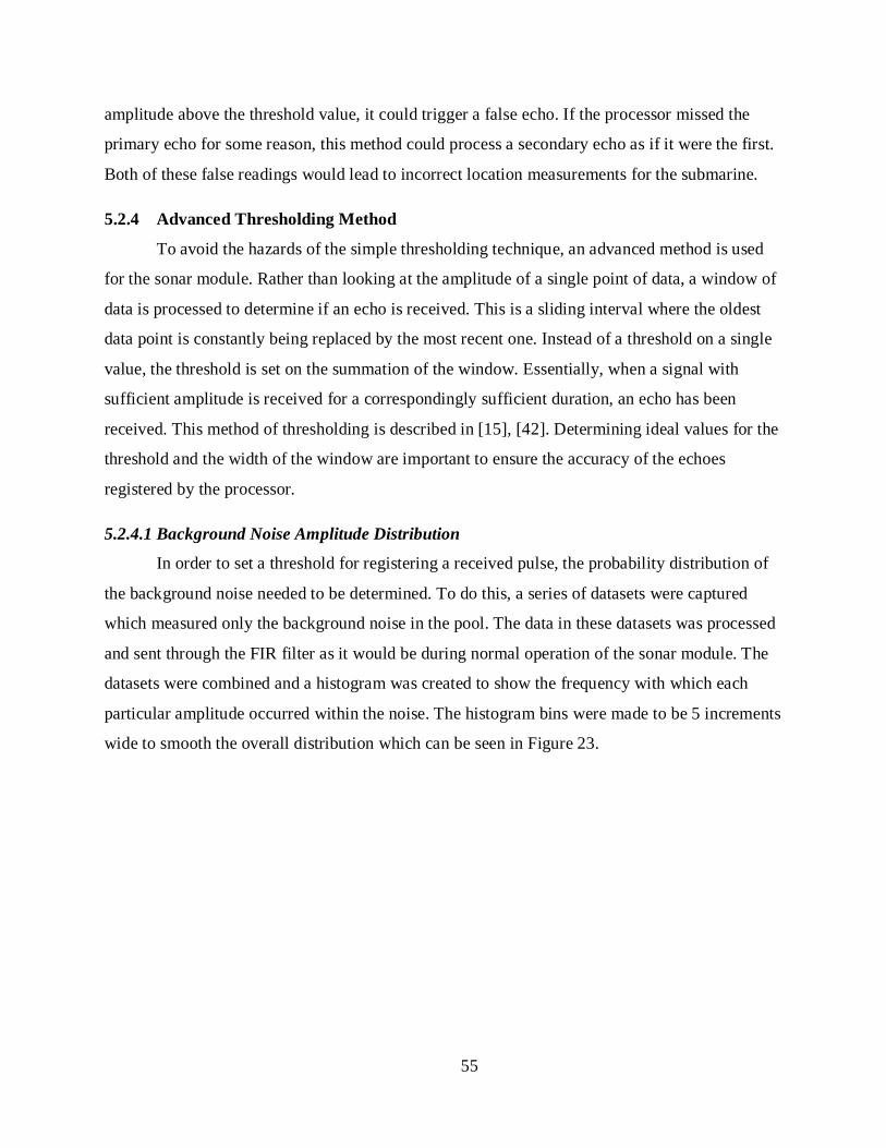
55
amplitude above the threshold value, it could trigger a false echo. If the processor missed the
primary echo for some reason, this method could process a secondary echo as if it were the first.
Both of these false readings would lead to incorrect location measurements for the submarine.
5.2.4 Advanced Thresholding Method
To avoid the hazards of the simple thresholding technique, an advanced method is used
for the sonar module. Rather than looking at the amplitude of a single point of data, a window of
data is processed to determine if an echo is received. This is a sliding interval where the oldest
data point is constantly being replaced by the most recent one. Instead of a threshold on a single
value, the threshold is set on the summation of the window. Essentially, when a signal with
sufficient amplitude is received for a correspondingly sufficient duration, an echo has been
received. This method of thresholding is described in [15], [42]. Determining ideal values for the
threshold and the width of the window are important to ensure the accuracy of the echoes
registered by the processor.
5.2.4.1 Background Noise Amplitude Distribution
In order to set a threshold for registering a received pulse, the probability distribution of
the background noise needed to be determined. To do this, a series of datasets were captured
which measured only the background noise in the pool. The data in these datasets was processed
and sent through the FIR filter as it would be during normal operation of the sonar module. The
datasets were combined and a histogram was created to show the frequency with which each
particular amplitude occurred within the noise. The histogram bins were made to be 5 increments
wide to smooth the overall distribution which can be seen in Figure 23.
56
Figure 23: The distribution of the amplitude of the filtered noise in the WPI pool.
5.2.4.2 Calculation of Summation Window Width and the Threshold Value
The threshold value used by the processor to determine if an echo has been received is of
critical importance and should not be chosen arbitrarily. If the threshold is too low, the
background noise in the tank could trigger false returns. On the other hand, if the threshold is too
high, some of the received echoes may fall below the threshold and would be missed. The
threshold and the window over which the received data is integrated must be chosen to minimize
the probability of false alarm and the probability of missed detection.
5.2.4.2.1 Summation Window Width
The summation window width was determined by examining the raw data from an
echoed pulse received through the sonar module. After receiving several different echoes at
varying distances, it was determined that the filtered ADC signal is the highest for three ADC
cycles when the echo is received. This makes sense because the width of the transmitted signal is
around 1.5 ms and each ADC cycle is about 650 µs. Unless things line up perfectly, it is logical
that the received pulse will span three ADC cycles. The summation window was consequently
0
50
100
150
200
250
300
350
400
450
500
4 48 92 136
180
224
268
312
356
400
444
488
532
576
620
664
708
752
796
840
884
928
972
Freq
uenc
y, #
of s
ampl
es
Amplitude
Frequency

57
chosen to be three samples wide to best capture a single return pulse and also reduce
computation time.
5.2.4.2.2 Determining the Threshold Value
Once the width of the summation window was decided, a threshold for the integration
over this window needed to be determined. In order to determine the best threshold for
measuring distances, a series of 11 thresholds were tested to determine how well they performed.
The sonar module was placed in the pool facing one of the walls 8.86 meters away. It was not
disturbed during any of the data collection so the distance would be fixed. For each potential
threshold, a series of 6000 distance measurements were gathered to establish the distribution.
A modified version of the transmit/receive program was created which would log the
measured distance for a series of pulses in RAM which could later be retrieved and processed on
a PC. Each pulse is separated by a delay time to allow the previous signal to attenuate before
another is sent. The program was tuned to an acceptable data collection rate where 1500 distance
measurements could be gathered in 30-45 seconds, depending on the distance being measured.
In Section 5.2.4.1, the distribution of the noise showed that the majority of the filtered
noise has amplitude less than 500, so the threshold increments began at 1500. The thresholds
tested were from 1500 to 3000 at 150 point increments. The 1500 measurements obtained by the
data collection program nearly fill all the memory available on the MSP430, so the program was
run multiple times at each potential threshold to get 6000 data points.
When the data was gathered, a histogram was created to show how often a given distance
measurement occurred. An example of one of these histograms is shown in Figure 24. The
histograms for all 11 thresholds tested are in Appendix G – Threshold Determination
Experiments.

58
Figure 24: Example of the distance measurement distribution for a threshold of 1800.
With the histograms generated for each threshold, the data were analyzed. At thresholds
lower than 2100, the largest frequency of returns occurs at a shorter distance than is actually
being measured. This phenomenon makes sense, because with a lower threshold there is a greater
potential for the noise to be high enough to trigger an early response. What are more concerning
are the distance measurements which are much shorter than the actual distance. These erroneous
distance measurements would lead to large errors in the calculated position of the vehicle. These
errors stop occurring at thresholds above 1800 because the magnitude of the noise is no longer
large enough to trigger a false alarm.
After these initial reactions, the data were further analyzed to determine the percentage of
distance measurements which yielded accurate results. In addition to this, the percentages of
measurements which were within 5 and 10 cm of the true distance were also calculated. The
results of these calculations can be found in Table 4. These data were used to decide upon a
threshold of 2100, which is highlighted in the table. A threshold of 2100 had the highest
0
200
400
600
800
1000
1200
1400
1600
1800
20005
635
1265
1895
2525
3155
3785
4415
5045
5675
6305
6935
7565
8195
8825
9455
1008
510
715
1134
511
975
1260
513
235
1386
514
495
Freq
uenc
y
Distance measured, mm
Distance Measurement Distribution for Threshold = 1800
Threshold = 1800
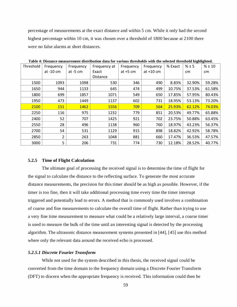
59
percentage of measurements at the exact distance and within 5 cm. While it only had the second
highest percentage within 10 cm, it was chosen over a threshold of 1800 because at 2100 there
were no false alarms at short distances.
5.2.5 Time of Flight Calculation
The ultimate goal of processing the received signal is to determine the time of flight for
the signal to calculate the distance to the reflecting surface. To generate the most accurate
distance measurements, the precision for this timer should be as high as possible. However, if the
timer is too fine, then it will take additional processing time every time the timer interrupt
triggered and potentially lead to errors. A method that is commonly used involves a combination
of coarse and fine measurements to calculate the overall time of flight. Rather than trying to use
a very fine time measurement to measure what could be a relatively large interval, a coarse timer
is used to measure the bulk of the time until an interesting signal is detected by the processing
algorithm. The ultrasonic distance measurement systems presented in [44], [45] use this method
where only the relevant data around the received echo is processed.
5.2.5.1 Discrete Fourier Transform
While not used for the system described in this thesis, the received signal could be
converted from the time domain to the frequency domain using a Discrete Fourier Transform
(DFT) to discern when the appropriate frequency is received. This information could then be
Table 4: Distance measurement distribution data for various thresholds with the selected threshold highlighted. Threshold Frequency
at -10 cm Frequency at -5 cm
Frequency at Exact Distance
Frequency at +5 cm
Frequency at +10 cm
% Exact % ± 5 cm
% ± 10 cm
1500 1093 1098 530 346 490 8.83% 32.90% 59.28% 1650 944 1133 645 474 499 10.75% 37.53% 61.58% 1800 699 1857 1071 549 650 17.85% 57.95% 80.43% 1950 473 1449 1137 602 731 18.95% 53.13% 73.20% 2100 151 1462 1556 709 564 25.93% 62.12% 74.03% 2250 116 975 1232 779 851 20.53% 49.77% 65.88% 2400 52 707 1425 921 702 23.75% 50.88% 63.45% 2550 28 496 1138 960 760 18.97% 43.23% 56.37% 2700 54 531 1129 915 898 18.82% 42.92% 58.78% 2850 2 263 1048 881 660 17.47% 36.53% 47.57% 3000 5 206 731 774 730 12.18% 28.52% 40.77%
60
used to calculate the phase shift between the transmitted and received signals to aid in the TOF
measurement or to determine the vehicle velocity relative to the reflected surface. A DFT is used
in [46] to combine simple TOF and phase-shifting methods for increased accuracy.
The tradeoff with using a method such as this is the additional computational time
necessary for the DFT. This might be acceptable for larger and more powerful systems, but the
MSP430 would not be able to do this processing in real time. To use this method, the entire
received pulse would need to be stored in memory and processed after sufficient time has passed
for the signal to attenuate. There is not enough RAM available on the MSP430, so this data
would need to be moved to the Flash memory, further increasing the computation time. Because
of the desire for a more timely response, the window summation method described above is
employed for the sonar module.
5.2.5.2 Measurement Precision
The precision of the TOF measurements is limited by the sampling rate of the ADC.
Since the ADC samples the signal at discrete times, the arrival time for any signal arriving
between samples is not accurately determined. Below are the calculations for the minimum
resolvable time and the corresponding minimum resolvable distance based upon the chosen ADC
sampling rate.
∆𝐼𝐼 = 1
𝑓𝑓𝐼𝐼𝑊𝑊𝐼𝐼𝑎𝑎𝑉𝑉𝐼𝐼=
115429 𝑆𝑆𝐻𝐻
= 64.81𝜇𝜇𝐼𝐼
∆𝑑𝑑 = ∆𝐼𝐼 ∗𝐼𝐼2
= 4.81 𝐼𝐼𝐼𝐼
To provide the most up to date position information to the submarine, the amount of time
spent processing data and transmitting it back to the main vehicle processor must be minimized.
If we tried to store and process the entire received signal on the MSP430 it would take a lot of
extra processing time. Likewise if all of the received data were transmitted to the PC/104 for
processing, the transmitting time would use valuable time. To increase the speed of the data
processing, only a small window of the signal is stored at any given time. If this window does
not satisfy the signal processing criteria, the oldest data piece is removed and the newest data
from the ADC is shifted into the window. Once the summation of the data within this sliding
window reaches the threshold, a pulse has been received and the distance can be calculated. With
61
this method, the processor only needs to perform simple calculations each time the interrupt
triggers and the only data that needs to be transmitted back to the PC/104 is the final measured
distance. The width of this summation window and the value of the threshold are determined in
Section 5.2.4.2.
5.2.5.3 Calculation of Time of Flight and Distance to Target
With a properly defined threshold value, it is fairly certain that when the signal passes
that threshold, an echo has been received. When the threshold is passed, the timers and ADC are
stopped and the time of flight is calculated. The calculations for the time of flight and the
distance to the reflecting object are shown below.
𝐼𝐼𝑓𝑓𝑉𝑉𝑟𝑟𝑓𝑓ℎ𝐼𝐼 = 𝐼𝐼𝐼𝐼𝑉𝑉𝑊𝑊𝐼𝐼𝐼𝐼𝐼𝐼 + 𝐼𝐼𝑓𝑓𝑟𝑟𝐼𝐼𝐼𝐼
𝑑𝑑𝐼𝐼𝑊𝑊𝐼𝐼𝑓𝑓𝐼𝐼𝐼𝐼 =𝐼𝐼 ∗ 𝐼𝐼𝑓𝑓𝑉𝑉𝑟𝑟𝑓𝑓ℎ𝐼𝐼
2
The time of flight is calculated using the sum of the coarse and fine time measurements. This
time is then multiplied by the speed of sound in water, c, to get the total distance traveled.
Finally, this value is divided by two to yield the desired distance measurement between the
submarine and the reflecting surface.
5.3 Overall Signal Processing Algorithm The flow chart in Figure 25 illustrates the flow of information as it is transmitted,
received, and processed by the MSP430. First, the signal is generated and transmitted by the
transducer. After transmission, the transducer switches to receive mode and the incoming signals
are processed. They go through hardware processing first before being converted to a digital
signal and stored in the MSP430. The software then processes the signal to find an echo which
crosses the threshold. Once the threshold is reached, the processor determines the time-of-flight
and calculates the corresponding distance which can then be sent to the submarine’s main
computer.
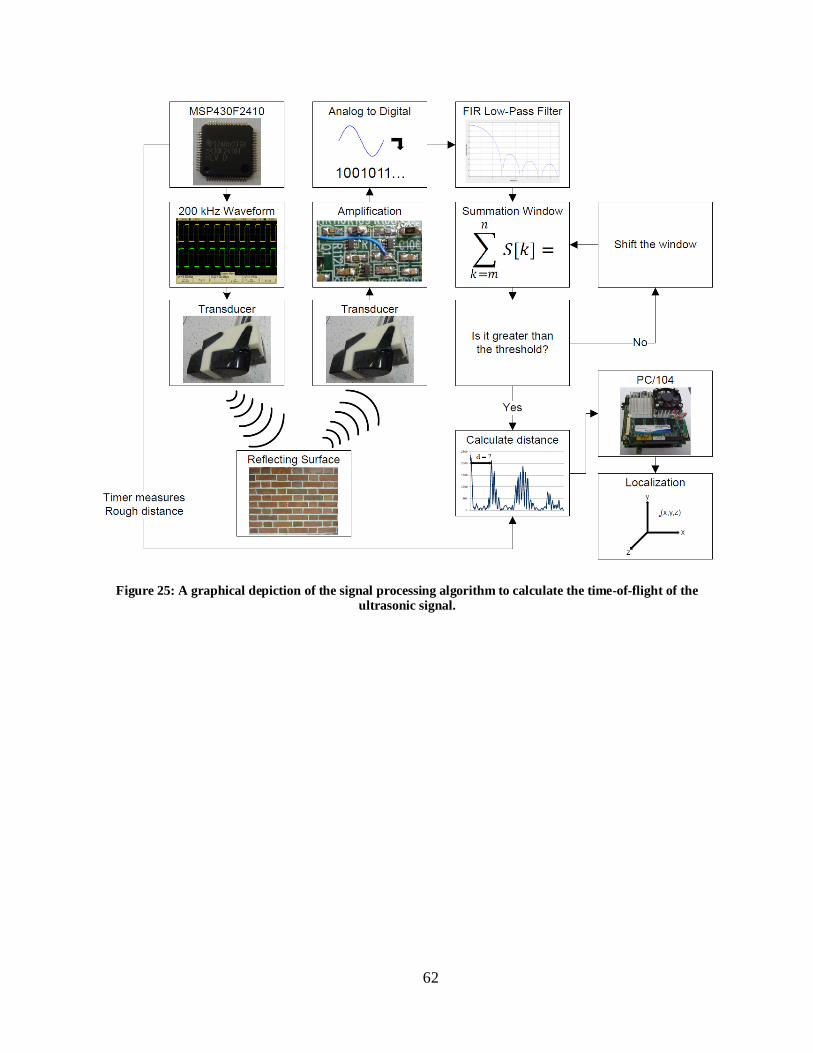
62
Figure 25: A graphical depiction of the signal processing algorithm to calculate the time-of-flight of the
ultrasonic signal.

63
6 Trigonometric Submarine Localization The sonar module presented in this thesis uses three distance measurements from
ultrasonic transducers in conjunction with the yaw, pitch, and roll angles measured by the
submarine sensors to determine the submarine position in a pool or tank. Along with these sensor
measurements, the submarine requires prior knowledge of the tank geometry including the depth
profile if it is not of constant depth. For the purposes of this thesis, a tank with a rectangular
horizontal cross section and a depth which varies with position is considered. Using these data,
the submarine can autonomously determine its three dimensional position within the tank in most
situations. When faced with one of the situations where the geometric solution does not work,
other methods can be employed to estimate the position until it can be measured again. This
algorithm assumes that the distance measurements received from the sonar module are from a
single reflection off a surface directly in the path of each sensor. This assumption may not be
valid for all measurements, and the method for handling this is discussed in Section 6.3.2.
Another assumption made with this iteration of the algorithm is that the roll and pitch
angles of the submarine are minimal. In essence, the submarine is assumed to be horizontal to
within 3-4 degrees. Larger angles could cause the ultrasonic sensors to measure an unintended
surface and the mathematics will not work. It is also assumed that the submarine will not travel
deep enough where one of the horizontal beams will reflect off of the bottom surface of the pool.
Future versions of this algorithm will seek to operate without these assumptions.
To simplify the trigonometry and calculations which the computer must perform, the first
step in the process is to project the three distance vectors measured with the transducers onto a
new coordinate system. The global coordinate system for the tank is placed at one corner of the
pool with the x-y plane corresponding to the surface of the water. The positive z axis extends
from the water level downwards and is equivalent to the depth of the submarine. The x and y
axis transducer measurements are projected onto the horizontal plane, with respect to the tank,
and the z axis transducer measurement is projected onto an axis normal to this plane. Below are
the projection equations used for this projection portion of the algorithm.
𝑑𝑑𝑎𝑎1 = 𝑑𝑑𝐼𝐼1 cos(𝜑𝜑)
𝑑𝑑𝑎𝑎2 = 𝑑𝑑𝐼𝐼2 cos(𝜌𝜌)

64
𝑑𝑑𝑎𝑎3 = 𝑑𝑑𝐼𝐼3 cos(𝜑𝜑) cos(𝜌𝜌)
The subscripts 𝐼𝐼 and 𝑎𝑎 correspond to the measured and projected distances respectively. The
angles 𝜌𝜌 and 𝜑𝜑 refer to the roll and pitch angle of the vehicle with respect to the fixed global
coordinate system. Throughout the remainder of this chapter, the sides of the tank will be
referenced by their position in this horizontal projection: left side, top side, right side, and lower
side.
Once the measurements are in this coordinate system, the same set of rules for
determining position can be applied regardless of the orientation of the vehicle. The situations
presented in this chapter are grouped into four orientations, based on the four possible quadrants
in which the yaw angle can lie. The yaw angle is measured between vector created by the
horizontal projection of the distance 𝑑𝑑𝑎𝑎1 and the positive x axis of the global coordinate system.
Please note that the coordinate system used for these calculations is not standard because the y-
axis is flipped. Figure 26 below shows the quadrants which correspond to each orientation.
Figure 26: Depiction of the coordinate and quadrant systems for the pool.
For each orientation, there are two sub cases which depend on which sides of the tank intersect
with the ultrasonic beams. There are also some cases where one of the coordinates cannot be

65
measured accurately. These singular situations, which will be explained later in Section 6.3, can
be correctly identified by the algorithm and then processed accordingly to determine the location
of the sub. Section 6.3 also explains some potential solutions for when the submarine finds itself
in one of these circumstances.
Section 6.1 explains the algorithm calculations for the first orientation in detail. Because
the calculations for the remaining three orientations are very similar, they are not discussed in the
main body of this thesis. The figures and equations which correspond to these orientations can be
found in Appendix H – Localization Algorithm Mathematics.
6.1 Orientation 1 The first orientation corresponds to a yaw angle which lies in the first quadrant of the
coordinate system. For any given orientation, there are four theoretical combinations of the sides
of the tank with which the sonar beams can intersect. The beams can intersect either two adjacent
sides, a different set of adjacent sides, two opposite sides, or the same side. These are depicted in
Figure 27. Both situations where the beams intersect with adjacent sides, the top two, can be
solved using the equations in this section, while the other two cases, the bottom two, are singular
and cannot be completely solved. The problem becomes finding a method of differentiating
between these cases with only the orientation of the vehicle and the projected distances known.
Figure 27: The four potential situations the submarine can be in for any given angle in orientation 1.
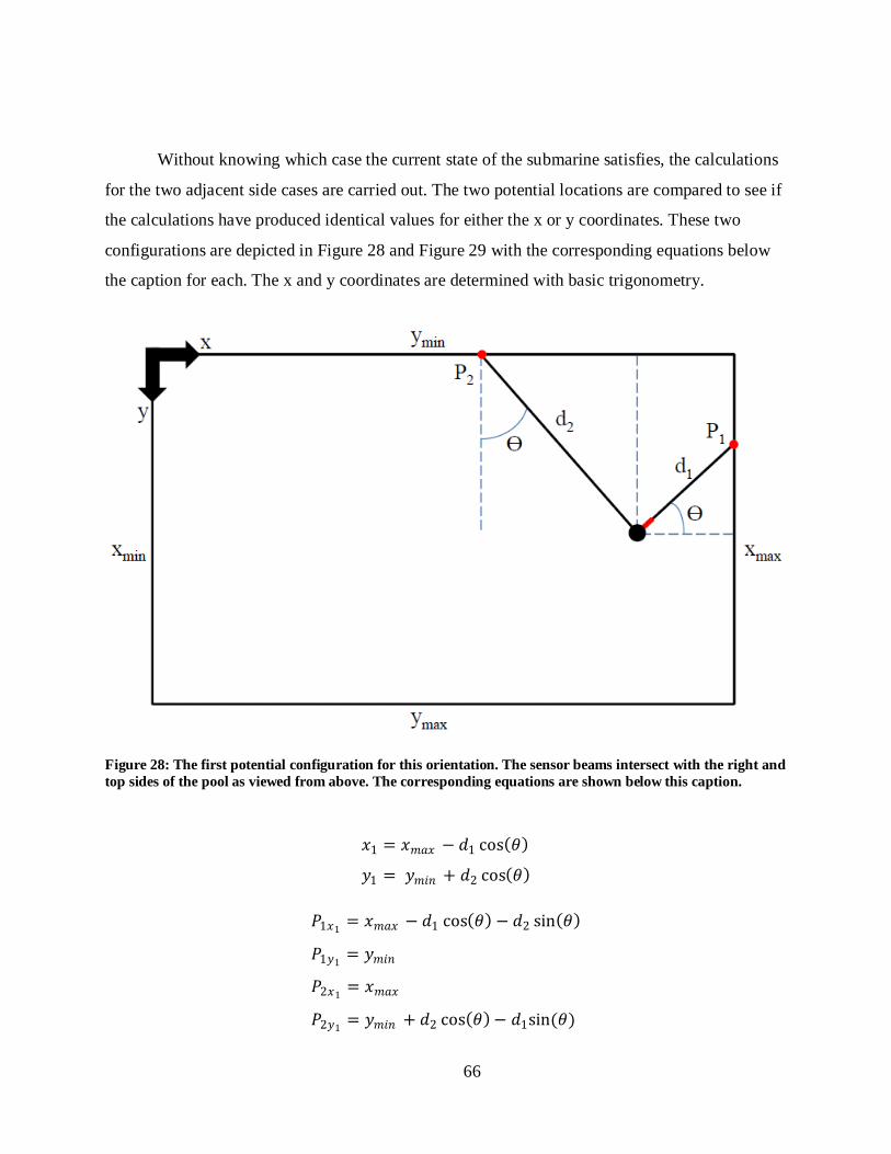
66
Without knowing which case the current state of the submarine satisfies, the calculations
for the two adjacent side cases are carried out. The two potential locations are compared to see if
the calculations have produced identical values for either the x or y coordinates. These two
configurations are depicted in Figure 28 and Figure 29 with the corresponding equations below
the caption for each. The x and y coordinates are determined with basic trigonometry.
Figure 28: The first potential configuration for this orientation. The sensor beams intersect with the right and top sides of the pool as viewed from above. The corresponding equations are shown below this caption.
𝑥𝑥1 = 𝑥𝑥𝐼𝐼𝑊𝑊𝑥𝑥 − 𝑑𝑑1 cos(𝜃𝜃)
𝑠𝑠1 = 𝑠𝑠𝐼𝐼𝑟𝑟𝐼𝐼 + 𝑑𝑑2 cos(𝜃𝜃)
𝑃𝑃1𝑥𝑥1 = 𝑥𝑥𝐼𝐼𝑊𝑊𝑥𝑥 − 𝑑𝑑1 cos(𝜃𝜃) − 𝑑𝑑2 sin(𝜃𝜃)
𝑃𝑃1𝑠𝑠1 = 𝑠𝑠𝐼𝐼𝑟𝑟𝐼𝐼
𝑃𝑃2𝑥𝑥1 = 𝑥𝑥𝐼𝐼𝑊𝑊𝑥𝑥
𝑃𝑃2𝑠𝑠1 = 𝑠𝑠𝐼𝐼𝑟𝑟𝐼𝐼 + 𝑑𝑑2 cos(𝜃𝜃)− 𝑑𝑑1sin(𝜃𝜃)
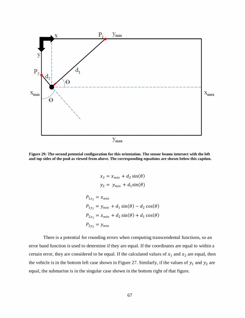
67
Figure 29: The second potential configuration for this orientation. The sensor beams intersect with the left and top sides of the pool as viewed from above. The corresponding equations are shown below this caption.
𝑥𝑥2 = 𝑥𝑥𝐼𝐼𝑟𝑟𝐼𝐼 + 𝑑𝑑2 sin(𝜃𝜃)
𝑠𝑠2 = 𝑠𝑠𝐼𝐼𝑟𝑟𝐼𝐼 + 𝑑𝑑1sin(𝜃𝜃)
𝑃𝑃1𝑥𝑥2 = 𝑥𝑥𝐼𝐼𝑟𝑟𝐼𝐼
𝑃𝑃1𝑠𝑠2 = 𝑠𝑠𝐼𝐼𝑟𝑟𝐼𝐼 + 𝑑𝑑1 sin(𝜃𝜃) − 𝑑𝑑2 cos(𝜃𝜃)
𝑃𝑃2𝑥𝑥2 = 𝑥𝑥𝐼𝐼𝑟𝑟𝐼𝐼 + 𝑑𝑑2 sin(𝜃𝜃) + 𝑑𝑑1 cos(𝜃𝜃)
𝑃𝑃2𝑠𝑠2 = 𝑠𝑠𝐼𝐼𝑟𝑟𝐼𝐼
There is a potential for rounding errors when computing transcendental functions, so an
error band function is used to determine if they are equal. If the coordinates are equal to within a
certain error, they are considered to be equal. If the calculated values of 𝑥𝑥1 and 𝑥𝑥2 are equal, then
the vehicle is in the bottom left case shown in Figure 27. Similarly, if the values of 𝑠𝑠1 and 𝑠𝑠2 are
equal, the submarine is in the singular case shown in the bottom right of that figure.

68
If the calculations pass this first check and the submarine is not in a singular situation, we
can move on to determining which set of equations is valid for the current state of the robot. To
do this, the points at which the axes of the sonar beams intersect with the sides of the pool are
calculated. With these calculations, one set of equations will produce intersection points which
lie on the boundaries of the tank and the other will yield at least one intersection point which is
outside the bounds of the pool. The set of equations which yields both intersection points on the
perimeter of the pool is set which corresponds to the location of the vehicle in the horizontal
plane.
With the x and y position of the submarine determined, the final step is to determine the z
position. In a tank with a fixed depth, the projected distance 𝑑𝑑𝑎𝑎3 can be simply subtracted from
the depth to determine the height below the water’s surface. For the more general case, where the
tank depth varies with position, the following equation is used.
𝐻𝐻 = 𝐻𝐻(𝑥𝑥, 𝑠𝑠) − 𝑑𝑑𝑎𝑎3
After examining the pool, the depth of the pool only varies along the length of the pool
and not along the width. This allows the previous equation to be simplified so it is only a
function of x.
𝐻𝐻 = 𝐻𝐻(𝑥𝑥) − 𝑑𝑑𝑎𝑎3
The equations used to determine the location of the submarine in the other three
quadrants of the horizontal plane are available in Appendix H – Localization Algorithm
Mathematics.
6.2 Determining the Tank Depth Profile The test tank for the sub@WPI project is the WPI swimming pool. The pool varies in
depth along its length, but has constant depth along its width. The depth profile is needed to
determine the function 𝐻𝐻(𝑥𝑥) mentioned in the previous section. Using the z-axis ultrasonic
transducer, the depth of the pool was measured at 50 centimeter increments along its length. Two
of the increments were not measured because the columns surrounding the pool were in the way.
The points at the shallowest end of the pool were not included because they were below the
measurable range of the sensor. A polynomial curve was fit to the measured points to create a
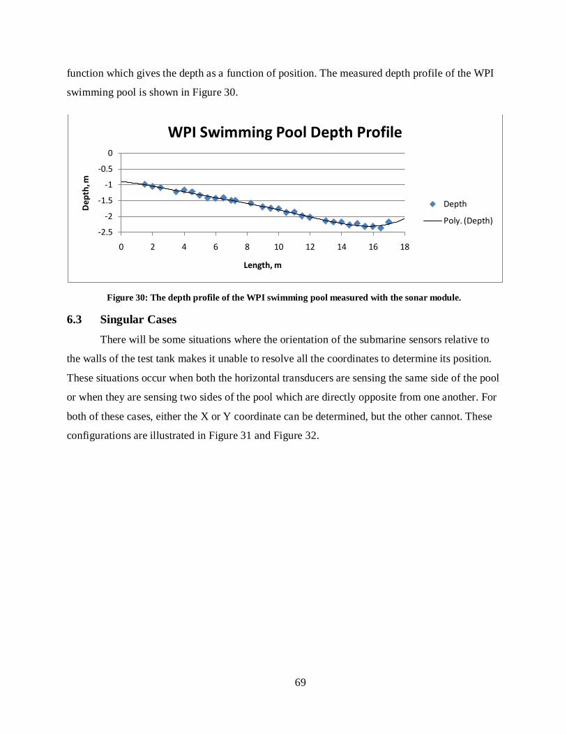
69
function which gives the depth as a function of position. The measured depth profile of the WPI
swimming pool is shown in Figure 30.
Figure 30: The depth profile of the WPI swimming pool measured with the sonar module.
6.3 Singular Cases There will be some situations where the orientation of the submarine sensors relative to
the walls of the test tank makes it unable to resolve all the coordinates to determine its position.
These situations occur when both the horizontal transducers are sensing the same side of the pool
or when they are sensing two sides of the pool which are directly opposite from one another. For
both of these cases, either the X or Y coordinate can be determined, but the other cannot. These
configurations are illustrated in Figure 31 and Figure 32.
-2.5
-2
-1.5
-1
-0.5
0
0 2 4 6 8 10 12 14 16 18
Dep
th, m
Length, m
WPI Swimming Pool Depth Profile
Depth
Poly. (Depth)
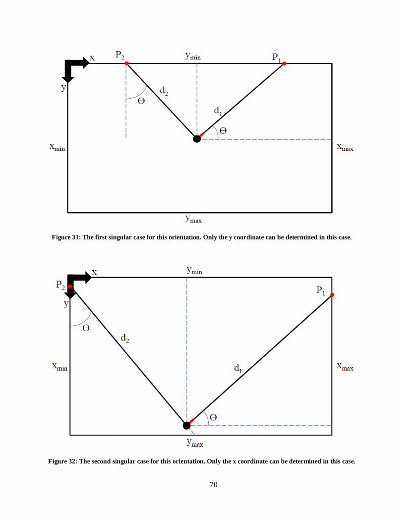
70
Figure 31: The first singular case for this orientation. Only the y coordinate can be determined in this case.
Figure 32: The second singular case for this orientation. Only the x coordinate can be determined in this case.

71
6.3.1 Localization with Singular Cases
There are a few potential ways in which the unknown coordinate can be determined. One
possible way which was investigated is using a secondary echo return to determine the distance
to one of the other surfaces in the tank. While this is technically possible in an ideal world, it
would require a detailed knowledge of the multipath behavior of the signal. The geometric
solution is based on the assumption that the received signal is reflected directly from the surface
in the direct line of sight of the sensor. This assumption can be made because the sensors have a
very narrow band of sensitivity. At 15 degrees to either side of the central axis of the sensor, the
sensitivity is at -20 dB and continues to decrease at larger angles. For this reason, there is a high
degree of confidence that any received echo is from a surface directly in line with the sensor axis
[31] ,[33]. In a noisy environment, it would not be reasonable to assume that this assumption will
hold for secondary echoes. Also, in order to use secondary echoes as part of the signal processing
algorithm, they would have to be measured for every cycle of the sensor. This would waste
valuable processing time and slow down the overall operation speed of the sensor.
In the event that the submarine finds itself in a situation where one of its coordinates is
unknown, it can be estimated using a technique known as feedback estimation. Essentially the
unknown coordinate will be estimated using its last known value and the vehicle’s dynamics
since that point. When the coordinate is able to be measured again, the estimate will be replaced
by the measured coordinate.
6.3.2 State Estimation Feedback
State estimation feedback is a common method used to estimate the state of a system
when the sensors used to measure the state have a high degree of noise. The state of the system
will be defined as the submarine’s three dimensional position within the pool. When the position
of the submarine determined by the algorithm is uncertain, the previous position of the
submarine and the submarine dynamics will be fed back and integrated to make an estimate of
the new position. This estimate will be updated when the submarine enters a determinate
configuration again [47].
6.4 Simulation of Submarine Localization
During the derivation of the algorithm described in the previous section, a simple
simulation program was written using Python to verify the calculations would yield the correct
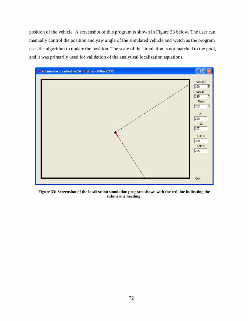
72
position of the vehicle. A screenshot of this program is shown in Figure 33 below. The user can
manually control the position and yaw angle of the simulated vehicle and watch as the program
uses the algorithm to update the position. The scale of the simulation is not matched to the pool,
and it was primarily used for validation of the analytical localization equations.
Figure 33: Screenshot of the localization simulation program shown with the red line indicating the
submarine heading.

73
7 Module Housing Design The sonar module is designed to be mounted on the underside of an autonomous
underwater vehicle, specifically the sub@WPI, which is currently under development as an
ongoing MQP in the CAN MUVE laboratory at WPI. Due to space constraints, the housing for
the module was designed to fit the three sensors in the smallest possible space. Considerations
for the manufacturability of the housing and necessary modifications to the sensors for mounting
were also taken into account. The housing was designed using the computer aided design
software package ProEngineer. An image of the assembly containing the housing and the sensors
can be found in Figure 34 below.
Figure 34: A ProEngineer CAD assembly of the module housing and the sensors.
Due to time constraints and the busy schedule of the machine shop, the part was designed
to be built using the school’s rapid prototyping machine, a Dimension 1200es SST [48]. The
machine deposits a thin filament of ABS plastic in a series of layers to create the 3D geometry of
the part. An acrylic based support structure is also deposited in each layer where there is
overhanging geometry. The support structure is later dissolved using a solution of Sodium
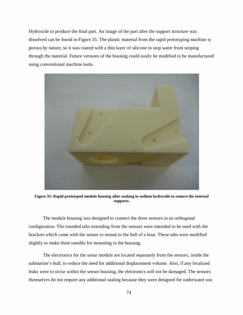
74
Hydroxide to produce the final part. An image of the part after the support structure was
dissolved can be found in Figure 35. The plastic material from the rapid prototyping machine is
porous by nature, so it was coated with a thin layer of silicone to stop water from seeping
through the material. Future versions of the housing could easily be modified to be manufactured
using conventional machine tools.
Figure 35: Rapid prototyped module housing after soaking in sodium hydroxide to remove the internal
supports.
The module housing was designed to connect the three sensors in an orthogonal
configuration. The rounded tabs extending from the sensors were intended to be used with the
brackets which came with the sensor to mount to the hull of a boat. These tabs were modified
slightly to make them useable for mounting to the housing.
The electronics for the sonar module are located separately from the sensors, inside the
submarine’s hull, to reduce the need for additional displacement volume. Also, if any localized
leaks were to occur within the sensor housing, the electronics will not be damaged. The sensors
themselves do not require any additional sealing because they were designed for underwater use.
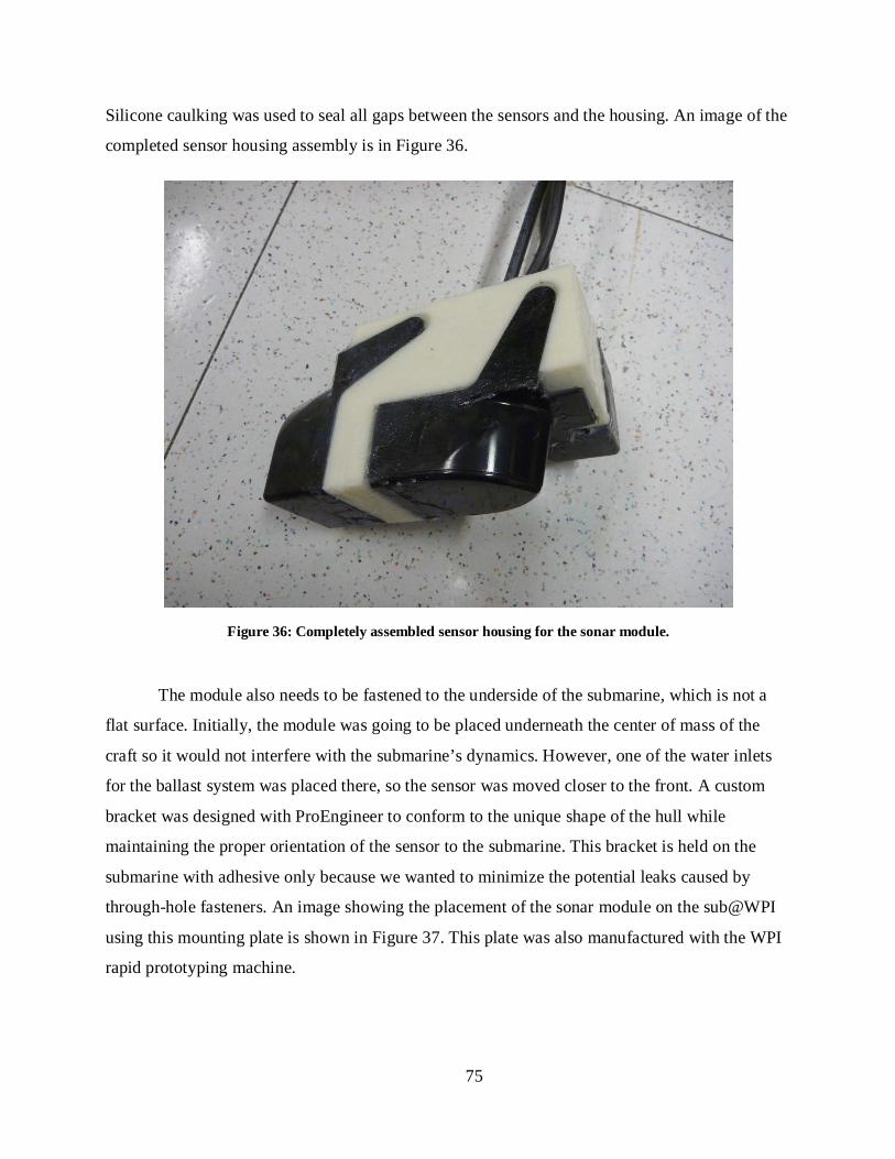
75
Silicone caulking was used to seal all gaps between the sensors and the housing. An image of the
completed sensor housing assembly is in Figure 36.
Figure 36: Completely assembled sensor housing for the sonar module.
The module also needs to be fastened to the underside of the submarine, which is not a
flat surface. Initially, the module was going to be placed underneath the center of mass of the
craft so it would not interfere with the submarine’s dynamics. However, one of the water inlets
for the ballast system was placed there, so the sensor was moved closer to the front. A custom
bracket was designed with ProEngineer to conform to the unique shape of the hull while
maintaining the proper orientation of the sensor to the submarine. This bracket is held on the
submarine with adhesive only because we wanted to minimize the potential leaks caused by
through-hole fasteners. An image showing the placement of the sonar module on the sub@WPI
using this mounting plate is shown in Figure 37. This plate was also manufactured with the WPI
rapid prototyping machine.
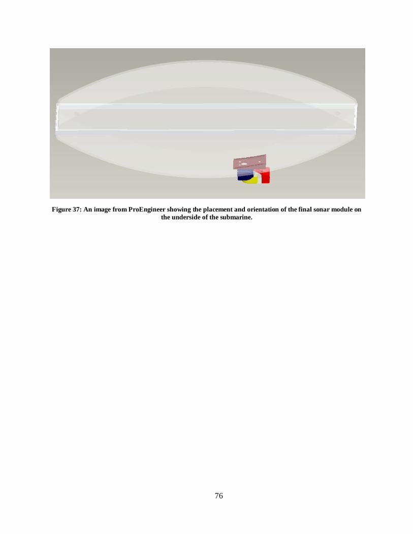
76
Figure 37: An image from ProEngineer showing the placement and orientation of the final sonar module on
the underside of the submarine.
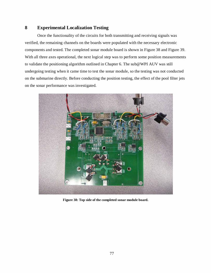
77
8 Experimental Localization Testing Once the functionality of the circuits for both transmitting and receiving signals was
verified, the remaining channels on the boards were populated with the necessary electronic
components and tested. The completed sonar module board is shown in Figure 38 and Figure 39.
With all three axes operational, the next logical step was to perform some position measurements
to validate the positioning algorithm outlined in Chapter 6. The sub@WPI AUV was still
undergoing testing when it came time to test the sonar module, so the testing was not conducted
on the submarine directly. Before conducting the position testing, the effect of the pool filter jets
on the sonar performance was investigated.
Figure 38: Top side of the completed sonar module board.
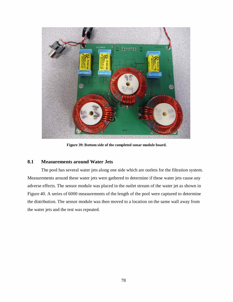
78
Figure 39: Bottom side of the completed sonar module board.
8.1 Measurements around Water Jets The pool has several water jets along one side which are outlets for the filtration system.
Measurements around these water jets were gathered to determine if these water jets cause any
adverse effects. The sensor module was placed in the outlet stream of the water jet as shown in
Figure 40. A series of 6000 measurements of the length of the pool were captured to determine
the distribution. The sensor module was then moved to a location on the same wall away from
the water jets and the test was repeated.
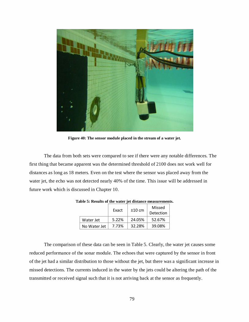
79
Figure 40: The sensor module placed in the stream of a water jet.
The data from both sets were compared to see if there were any notable differences. The
first thing that became apparent was the determined threshold of 2100 does not work well for
distances as long as 18 meters. Even on the test where the sensor was placed away from the
water jet, the echo was not detected nearly 40% of the time. This issue will be addressed in
future work which is discussed in Chapter 10.
Table 5: Results of the water jet distance measurements.
Exact ±10 cm Missed
Detection Water Jet 5.22% 24.05% 52.67% No Water Jet 7.73% 32.28% 39.08%
The comparison of these data can be seen in Table 5. Clearly, the water jet causes some
reduced performance of the sonar module. The echoes that were captured by the sensor in front
of the jet had a similar distribution to those without the jet, but there was a significant increase in
missed detections. The currents induced in the water by the jets could be altering the path of the
transmitted or received signal such that it is not arriving back at the sensor as frequently.
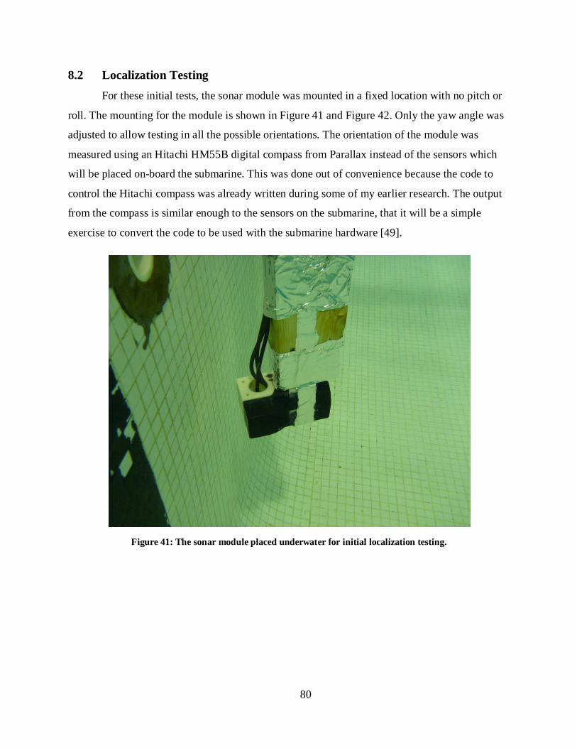
80
8.2 Localization Testing For these initial tests, the sonar module was mounted in a fixed location with no pitch or
roll. The mounting for the module is shown in Figure 41 and Figure 42. Only the yaw angle was
adjusted to allow testing in all the possible orientations. The orientation of the module was
measured using an Hitachi HM55B digital compass from Parallax instead of the sensors which
will be placed on-board the submarine. This was done out of convenience because the code to
control the Hitachi compass was already written during some of my earlier research. The output
from the compass is similar enough to the sensors on the submarine, that it will be a simple
exercise to convert the code to be used with the submarine hardware [49].
Figure 41: The sonar module placed underwater for initial localization testing.
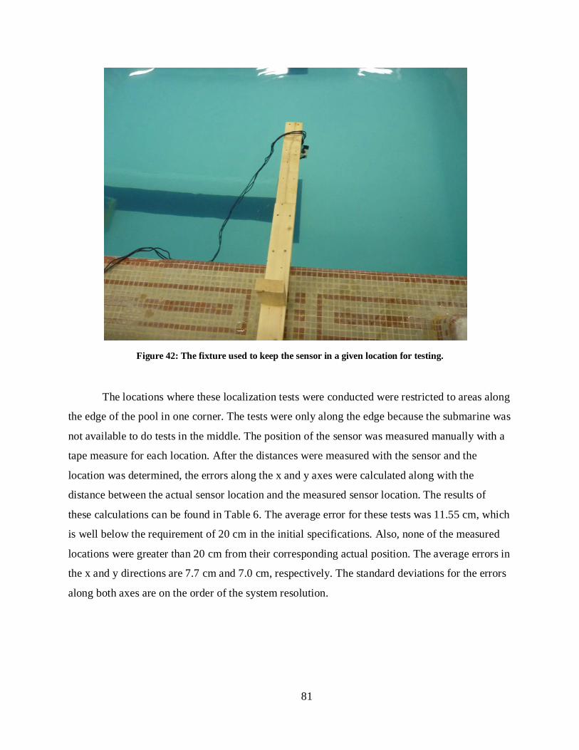
81
Figure 42: The fixture used to keep the sensor in a given location for testing.
The locations where these localization tests were conducted were restricted to areas along
the edge of the pool in one corner. The tests were only along the edge because the submarine was
not available to do tests in the middle. The position of the sensor was measured manually with a
tape measure for each location. After the distances were measured with the sensor and the
location was determined, the errors along the x and y axes were calculated along with the
distance between the actual sensor location and the measured sensor location. The results of
these calculations can be found in Table 6. The average error for these tests was 11.55 cm, which
is well below the requirement of 20 cm in the initial specifications. Also, none of the measured
locations were greater than 20 cm from their corresponding actual position. The average errors in
the x and y directions are 7.7 cm and 7.0 cm, respectively. The standard deviations for the errors
along both axes are on the order of the system resolution.
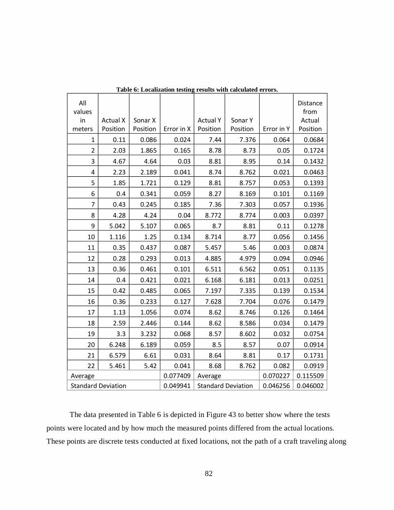
82
Table 6: Localization testing results with calculated errors.
All values
in meters
Actual X Position
Sonar X Position Error in X
Actual Y Position
Sonar Y Position Error in Y
Distance from
Actual Position
1 0.11 0.086 0.024 7.44 7.376 0.064 0.0684 2 2.03 1.865 0.165 8.78 8.73 0.05 0.1724 3 4.67 4.64 0.03 8.81 8.95 0.14 0.1432 4 2.23 2.189 0.041 8.74 8.762 0.021 0.0463 5 1.85 1.721 0.129 8.81 8.757 0.053 0.1393 6 0.4 0.341 0.059 8.27 8.169 0.101 0.1169 7 0.43 0.245 0.185 7.36 7.303 0.057 0.1936 8 4.28 4.24 0.04 8.772 8.774 0.003 0.0397 9 5.042 5.107 0.065 8.7 8.81 0.11 0.1278
10 1.116 1.25 0.134 8.714 8.77 0.056 0.1456 11 0.35 0.437 0.087 5.457 5.46 0.003 0.0874 12 0.28 0.293 0.013 4.885 4.979 0.094 0.0946 13 0.36 0.461 0.101 6.511 6.562 0.051 0.1135 14 0.4 0.421 0.021 6.168 6.181 0.013 0.0251 15 0.42 0.485 0.065 7.197 7.335 0.139 0.1534 16 0.36 0.233 0.127 7.628 7.704 0.076 0.1479 17 1.13 1.056 0.074 8.62 8.746 0.126 0.1464 18 2.59 2.446 0.144 8.62 8.586 0.034 0.1479 19 3.3 3.232 0.068 8.57 8.602 0.032 0.0754 20 6.248 6.189 0.059 8.5 8.57 0.07 0.0914 21 6.579 6.61 0.031 8.64 8.81 0.17 0.1731 22 5.461 5.42 0.041 8.68 8.762 0.082 0.0919
Average 0.077409 Average 0.070227 0.115509 Standard Deviation 0.049941 Standard Deviation 0.046256 0.046002
The data presented in Table 6 is depicted in Figure 43 to better show where the tests
points were located and by how much the measured points differed from the actual locations.
These points are discrete tests conducted at fixed locations, not the path of a craft traveling along
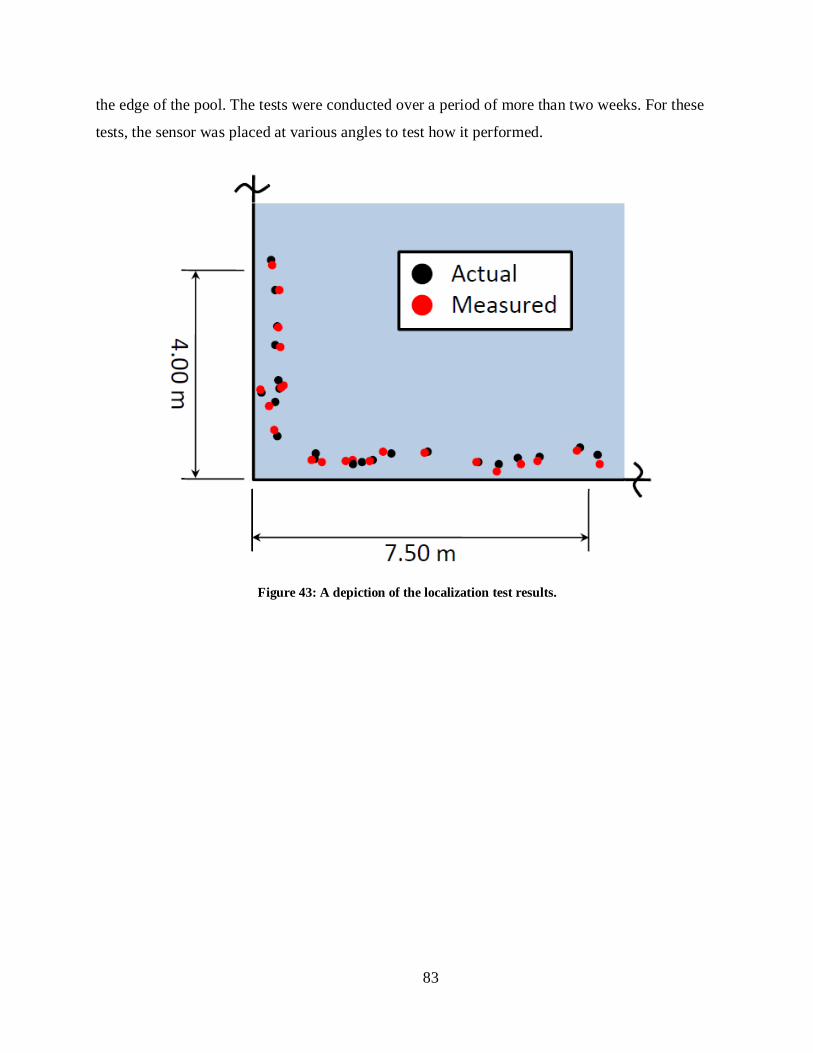
83
the edge of the pool. The tests were conducted over a period of more than two weeks. For these
tests, the sensor was placed at various angles to test how it performed.
Figure 43: A depiction of the localization test results.

84
9 Conclusions The research presented in this thesis resulted in the successful demonstration of a novel
localization system for use on experimental autonomous underwater vehicles. The module uses a
custom circuit board and readily available components to perform localization using ultrasonic
range finding within a bounded environment. A specialized algorithm was developed to use the
tri-axial ultrasonic measurements and the submarine orientation to calculate the absolute position
within a tank or pool. Unlike other positioning systems designed for testing at this scale, this
module does not require any external hardware, or the calibration which comes with that
hardware, in order to localize the craft. The chosen sampling rate of the analog to digital
convertor provides a range resolution of 4.8 cm. Testing has shown that the sensor is able to
resolve distances between 0.90 m and 20.50 m, which both satisfy the original design
requirements. With a total cost of less than $400, this module meets the cost requirement and
would be an excellent addition to any tank based experimental AUV project. It would be
especially suited for projects which need a positioning system to perform a SLAM algorithm.
As the design stands, there are obvious limitations in both the range and the resolution of
the module. This is one of the tradeoffs which was accepted with the development of this device
in order to keep costs low. We were not able to measure the maximum range of the system,
because it was longer than the longest distance in the pool. Even if we improved the hardware on
the sonar board, the range will not increase by much more because the signal will be near the
level of the background noise. The resolution of the system can be improved by using better
hardware in place of the MSP430. A faster processor and analog to digital convertor could
sample the data faster and potentially allow for implementation of the higher order FIR filter.
While these improvements would be welcome, the current module provides more than sufficient
measurements to localize the submarine.
The other main issue with the method used for this system’s design is the indeterminate
cases where the submarine location is unknown. A well placed beacon network could provide
complete localization coverage of a domain with better resolutions than the sonar module
developed in this thesis. The decrease in resolution is acceptable because the system is contained
entirely within the submarine and does not require setup and calibration time for each
experimentation session.

85
10 Recommendations and Future Work A working experimental version of a localization system has been demonstrated in this
thesis, but there is still work remaining to be done. There were a number of problems discovered
with the layout of the circuit during the development of the board. The schematics and board
layouts accompanying this document have been updated to reflect the changes necessary to make
the circuit function, but these changes should be verified. Also, the boards should be reviewed to
determine if there are any areas for improvement. One potential improvement would be to add
diodes to limit the voltage into the ADC so the components will not be subjected to high power
loads when a signal is reflected back at close range. After the design has been thoroughly
inspected, a new version of the board should be fabricated and tested.
The largest portion of work remaining for the sonar module is implementing the
algorithm presented in Chapter 6 in its final form so it can run automatically on the PC/104. This
will involve writing various functions which are able to be used within the framework of the
control code for the submarine. The necessary functions include polling the sonar module for
distance measurements, receiving distance measurements from the sonar module, processing the
obtained measurements according to the algorithm, and implementing a Kalman filter to estimate
the position of the submarine. The algorithm has been implemented in the localization simulation
program described in Section 6.4, but it will need to be altered to accept distances from the sonar
module.
The range resolution of the sonar module is currently limited by the sampling rate of the
analog to digital convertor. If one wants to improve the resolution in the future, a higher
performance microcontroller with a faster ADC will need to be implemented. This will likely
require a redesign of the sonar module board and possibly rewriting the sonar module control
code.
The threshold value for the sensor was determined experimentally in Section 5.2.4.2., but
it was later determined to be less than ideal for longer distances in the testing presented in
Section 8.1. It is already known that if the threshold is lowered it will cause incorrect readings
which are much shorter than the distance being measured. It might be beneficial to investigate
creating a threshold which varies as a function of time. Depending on how many ADC cycles
have passed, the threshold will decrease accordingly to allow the longer distances to be measured
86
with greater precision. A significant amount of testing would need to be conducted at various
distances in order for this method to be implemented.
The algorithm developed in Chapter 6 makes several assumptions in order to function
properly. Among these are the assumptions that the roll and pitch angles of the submarine are
minimal and that the depth of the submarine will not be too large so as to cause the horizontal
sensors to intersect with the bottom of the pool. Future iterations of the algorithm should seek to
extend the algorithm’s performance to the entire pool. Eventually the algorithm can potentially
be extended further to a tank with an arbitrary geometry.
The module developed in this thesis is a compact and simple localization system which
could benefit numerous research projects. Studies should be performed to determine the
marketability of this module to other research institutions and whether production would be
feasible. To make the localization system completely stand alone as a module, it might be
beneficial to investigate putting sensors for yaw, pitch, and roll on the board. This will increase
the cost of the module, but it would also make it useful to more vehicles which do not have those
sensors available.

87
11 Bibliography [1] Tritech International Ltd, Tritech PA200/PA500 Altimeters – Underwater Distance
Measurement, [Online], Available: http://www.tritech.co.uk/products/products-
pa200_pa500.htm.
[2] L. Stutters, H. Liu, C. Tiltman, and D.J. Brown, “Navigation technologies for
autonomous underwater vehicles,” Systems, Man, and Cybernetics, Part C: Applications and
Reviews, IEEE Transactions on, 38(4), pp.581–589, July 2008.
[3] Acroname Robotics, Hokuyo URG-04LX-UG01 Laser, http://www.acroname.com/
robotics/parts/R325-URG-04LX-UG01.html.
[4] MIT CSAIL, The Cricket Indoor Location System, http://cricket.csail.mit.edu/.
[5] L. L. Whitcomb, D. R. Yoerger, and H. Singh, “Combined Doppler/LBL based
navigation of underwater vehicles,” in Proc. Int. Symp. on Unmanned Untethered Submersible
Technology, 1999.
[6] J. Leonard, A. Bennett, C. Smith, and H. Feder, “Autonomous Underwater Vehicle
Navigation,” MIT Marine Robotics Laboratory Technical Memorandum, 98-1, 1998.
[7] M. Mandt, K. Gade, and B. Jalving, “Integrating DGPS-USBL positioning measurements
with inertial navigation in the HUGIN 3000 AUV”. Proc. 8th Saint Petersburg International
Conference on Integrated Navigation Systems, Saint Petersburg, Russia, May 2001.
[8] F. Thomas and L. Ros, “Revisiting trilateration for robot localization,” IEEE
Transactions on Robotics, 21(1), 2005, pp. 93-101.
[9] N. H. Kussat, C. D. Chadwell, R. Zimmerman, “Absolute positioning of an autonomous
underwater vehicle using GPS and acoustic measurements,” IEEE Journal of Oceanic
Engineering. Vol. 30, no. 1, Jan. 2005, pp. 153-164.
[10] J. Benesty, “Adaptive eigenvalue decomposition algorithm for passive acoustic source
localization,” J. Acoust. Soc. Am. 107, 384, 2000.

88
[11] S. A. L. Glegg, M. P. Olivieri, R. K. Coulson and S. M. Smith, “A passive sonar system
based on an autonomous underwater vehicle,” IEEE J. Oceanic Eng., vol. 26, 2001, pp. 700-710.
[12] P. Maxim, S. Hettiarachchi, W. Spears, D. Spears, J. Hamann, T. Kunkel, and C. Speiser,
“Trilateration localization for multi-robot teams,” In International Conference on Informatics in
Control, Automation, and Robotics, 4th International Workshop on Multi-Agent Robotic
Systems, 2008.
[13] R. Garcia, J. Batlle, X. Cufi, and J. Amat, “Positioning an underwater vehicle through
image mosaicking,” Proc. IEEE Int. Conf. on Robotics and Automation, Seoul, South Korea, part
3, 2001, pp. 2779–2784.
[14] N. Gracias, S. van der Zwaan, A. Bernardino, and J. Santos-Victor, “Mosaic based
navigation for autonomous underwater vehicles,” IEEE Journal of Oceanic Engineering, 28(4):
Oct. 2003, pp. 609-624.
[15] R. Eustice, “Large-area visually augmented navigation for autonomous underwater
vehicles,” Ph.D. dissertation, Massachusetts Institute of Technology/Woods Hole Oceanogr. Inst.
Joint Prog., Woods Hole, MA, Jun. 2005.
[16] P. Corke, C. Detweiler, M. Dunbabin, M. Hamilton, D. Rus, I. Vasilescu, “Experiments
with Underwater Robot Localization and Tracking”, In Proc. of IEEE International Conference
on Robotics and Automation, April 2007, pp 4556-4561.
[17] Evolution Robotics, Northstar Localization System, http://www.evolution.com/products/
northstar/.
[18] J. R. Solberg, K. M. Lynch, and M. A. MacIver, “Active Electrolocation for Underwater
Target Localization,” The International Journal of Robotics Research, 2008, 27: pp. 529-548.
[19] M. Denny, “Blip, ping and buzz: making sense of radar and sonar,” Baltimore, Maryland,
Johns Hopkins University Press, 2007, pp. 1-45, 240-242.
[20] A. Foessel, J. Bares, and W. Whittaker, “Three-dimensional map building with MMW
radar,” In Proc. of the 3rd International Conference on Field and Service Robotics, Helsinki,
Finland, June 2001.
89
[21] A. Goktogan, G. Brooker, and S. Sukkarieh, "A Compact Millimeter Wave Radar Sensor
for Unmanned Air Vehicles," presented at 4th International Conference on Field and Service
Robotics, Yamanashi, Japan, 2003.
[22] E. Jose and M. Adams, “Millimetre Wave RADAR Spectra Simulation and Interpretation
for Outdoor SLAM,” IEEE International Conference on Robotics & Automation, New Orleans,
USA, 2004.
[23] Acroname Robotics, Hokuyo UTM-30LX Laser, http://www.acroname.com/robotics/
parts/R314-HOKUYO-LASER4.html.
[24] H. Kondo and T. Ura, “Navigation of an AUV for investigation of underwater
structures,” Control Engineering Practice, Volume 12, Issue 12, Guidance and control of
underwater vehicles, Dec. 2004, pp. 1551-1559.
[25] Hagisonic, StarGazer Localization System, [Online], Available:
http://www.hagisonic.com/.
[26] J. Leonard and H. Durrant-Whyte, “Mobile robot localization by tracking geometric
beacons,” IEEE Trans. Robot. Automat., 7, (3), 1991, pp. 376–382.
[27] A. Matos, N. Cruz, A. Martins, and F. L. Pereira, “Development and Implementation of a
Low-Cost LBL Navigation System for an AUV,” Proceedings of the MTS/IEEE Oceans’99
Conference, Seattle, USA, 1999.
[28] M. Drumheller, “Mobile robot localization using sonar,” IEEE transactions on pattern
analysis and machine intelligence, March 1987, 9(2): pp. 325-332.
[29] R. David, M. French, B. Habin, and A. Kejriwal. “Design of Autonomous Underwater
Vehicle and Optimization of Hydrodynamic Properties and Control,” Major Qualifying Project,
Worcester Polytechnic Institute, 2009.
[30] A. R. Hambley, “Electrical Engineering: Principles and Applications,” 3rd ed., New York,
Pearson Education, 2005, pp. 632-686.

90
[31] Airmar Technology Corporation, Technical Data Catalog – 200A, [Online], Available:
http://www.airmar.com/.
[32] STMicroelectronics, STD30NF03L Datasheet, [Online], Available: http://www.st.com/
stonline/products/ literature/ds/6763/std30nf03l.pdf.
[33] Airmar Technology Corporation, Technical Data Catalog – 200BB, [Online], Available:
http://www.airmar.com/.
[34] D. Wilson and L. Liebermann, “Attenuation of Sound in Water,” J. Acoust. Soc. Am. 19,
286, 1947.
[35] National Physical Laboratory, “The speed an attenuation of sound,” 2008, [Online],
Available: http://www.kayelaby.npl.co.uk/general_physics/2_4/2_4_1.html.
[36] Federation of American Scientists, “Fundamentals of Naval Weapon Systems Chapter 8:
Principles of Underwater Sound,” [Online], Available: http://www.fas.org/man/dod-
101/navy/docs/fun/part08.htm.
[37] Texas Instruments, MSP430x2xx Family User’s Guide, [Online], Available:
http://focus.ti.com/lit/ug/ slau144e/slau144e.pdf, March 4, 2008.
[38] C. E. Shannon, “Communication in the presence of noise,” Proc. IRE, vol. 37, no. 1, pp.
10–21, Jan. 1949. See reprint (Classic Paper), Proc. IEEE, vol. 86, Feb. 1998, pp. 447–457.
[39] B. A. Shenoi. “Introduction to Digital Signal Processing and Filter Design,” New Jersey,
Wiley, 2005, pp. 250-259.
[40] J. G. Proakis and D. G. Manolakis, “Digital Signal Processing, Principles, Algorithms,
and Applications,” Englewood Cliffs, New Jersey, Prentice Hall, 1996, pp. 660-701.
[41] B. Barshan and R. Kuc, ‘‘A bat-like sonar system for obstacle localization,’’ IEEE Trans.
Syst. Man Cybern. 22, 1992, pp. 636–646.
[42] L. Kleeman and R. Kuc, “Sonar Sensing,” Springer Handbook of Robotics, 21, 2008, pp.
491-519.
91
[43] G. Andria, F. Attivissimo, and N. Giaquinto, “Digital signal processing techniques for
accurate ultrasonic sensor measurement,” Measurement, Volume 30, Issue 2, Sept. 2001, pp.
105-114.
[44] S. S. Huang, C. F. Huang, K. N. Huang, and M. S. Young, “A high accuracy ultrasonic
distance measurement system using binary frequency shift-keyed signal and phase detection,”
Rev. Sci. Instrum., 73, 3671, 2002.
[45] D. Marioli, C. Narduzzi, C. Offelli, D. Petri, E. Sardini, and A. Taroni, “Digital Time-of-
flight Measurement for Ultrasonic Sensors,” IEEE Transactions on Instrumentation and
Measurement. Vol. 41, No. 1, Feb. 1992, pp. 93-97.
[46] F. E. Gueuing, M. Varlan, C. E. Eugene, and P. Dupuis, “Accurate distance measurement
by an autonomous ultrasonic system combining time-of-flight and phase-shift methods,” IEEE
Trans. Instrum. Meas., vol. 46, Dec. 1997, pp. 1236–1240.
[47] C. T. Chen, “Linear System Theory and Design: Third Edition,” New York: Holt,
Rinehart, and Winston, 1999.
[48] Dimension Printing, Dimension 1200 Series Specs, [Online], Available:
http://www.dimensionprinting.com/ 3d-printers/printing-productspecs1200series.aspx.
[49] Parallax Inc., Hitachi HM55B Compass Module, [Online], Available:
http://www.parallax.com/Store/Microcontrollers/BASICStampModules/tabid/134/ProductID/98/
List/1/Default.aspx.
92
12 Appendices
12.1 Appendix A – Electrical Schematics
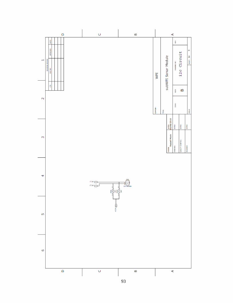
93
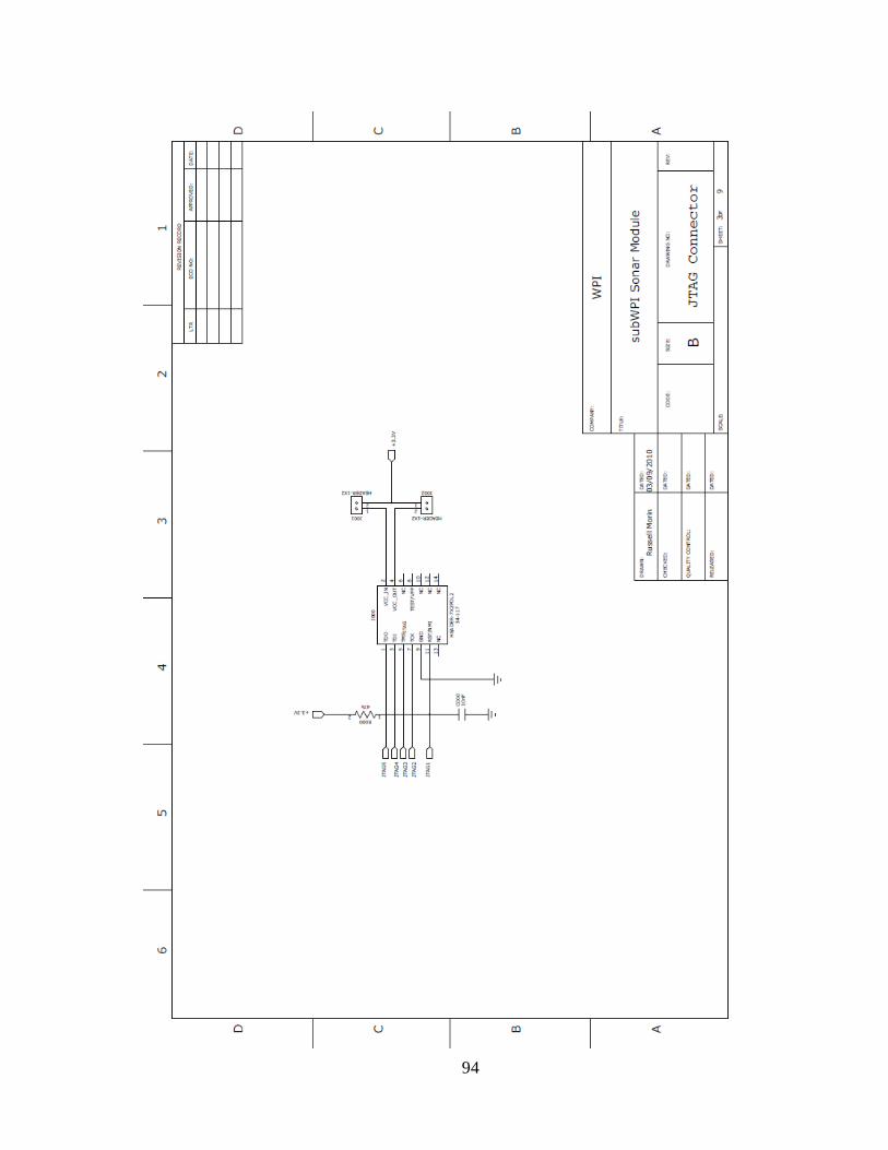
94
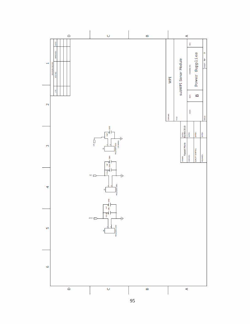
95
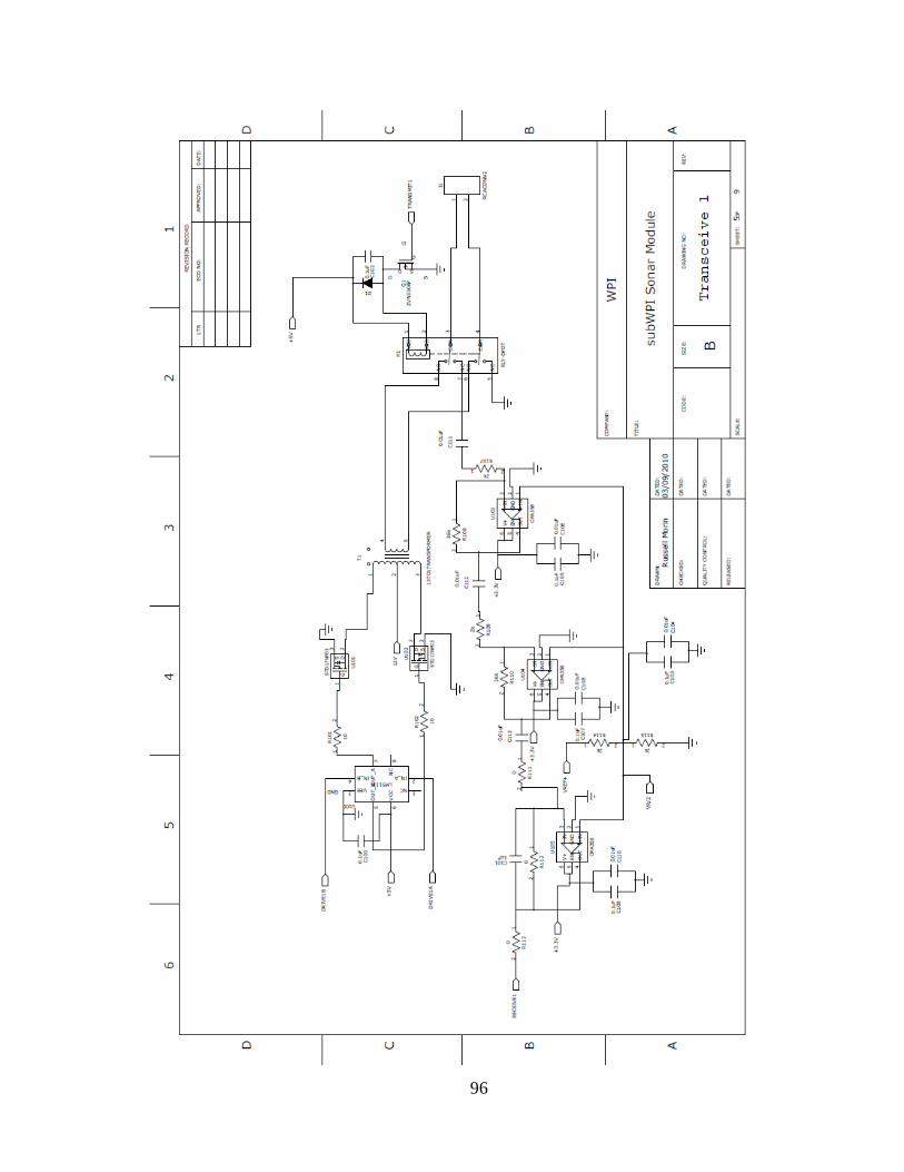
96
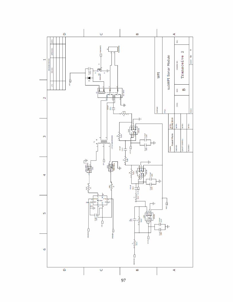
97
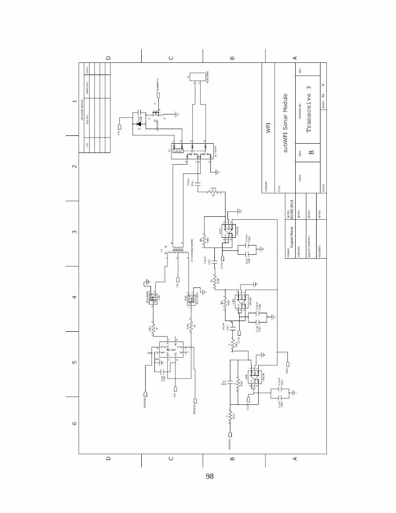
98
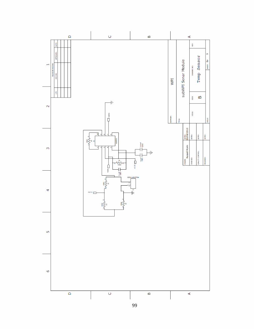
99
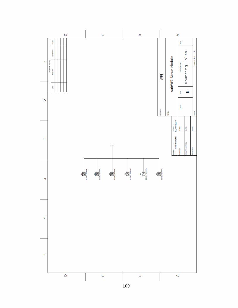
100
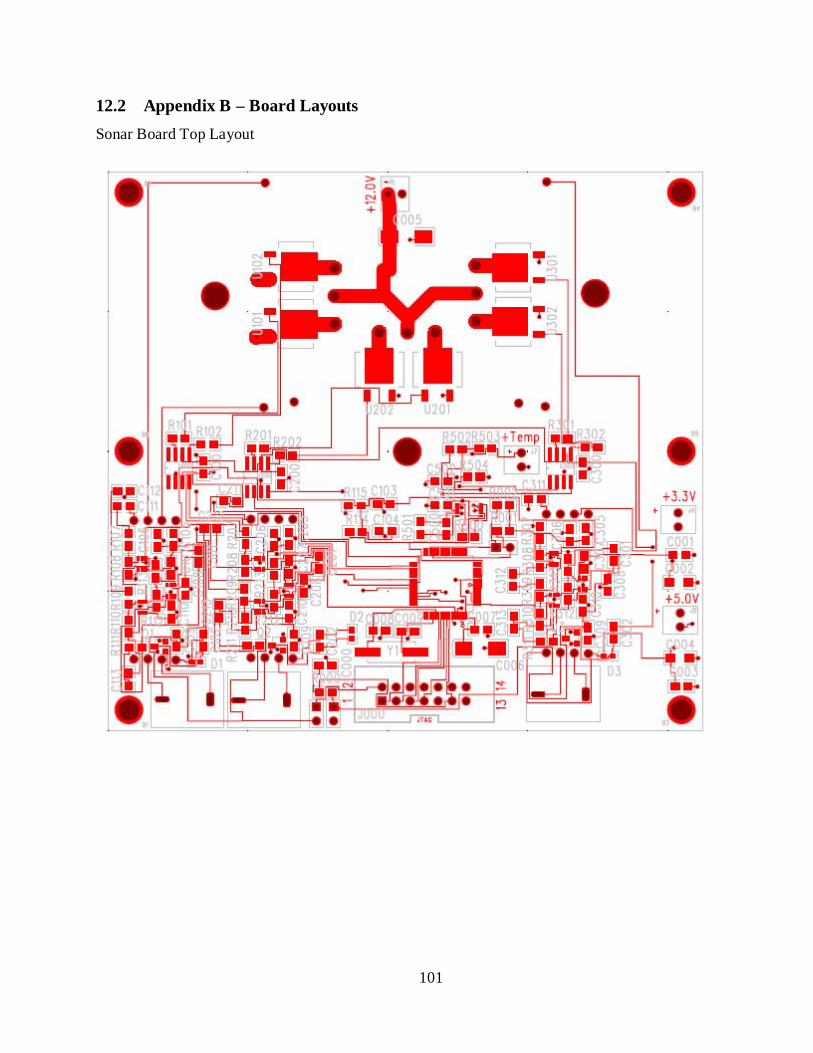
101
12.2 Appendix B – Board Layouts Sonar Board Top Layout
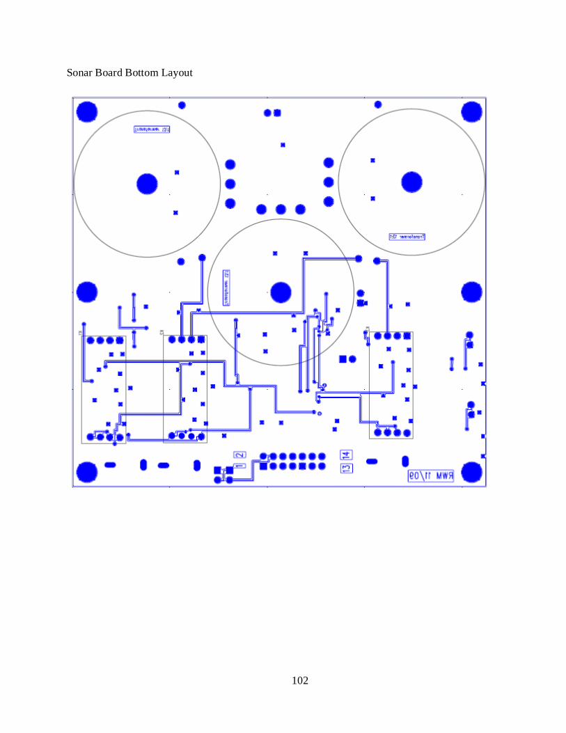
102
Sonar Board Bottom Layout
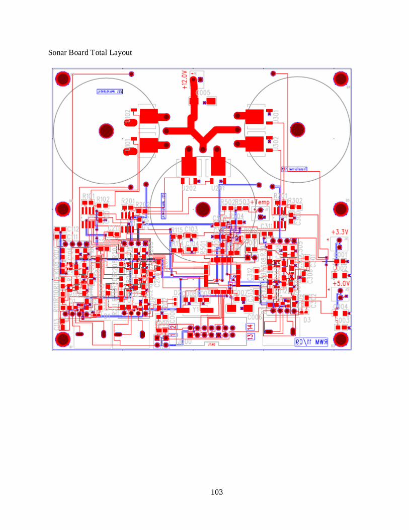
103
Sonar Board Total Layout
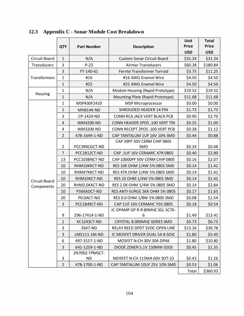
104
12.3 Appendix C - Sonar Module Cost Breakdown
QTY Part Number Description
Unit Price
Total Price
USD USD
Circuit Board 1 N/A Custom Sonar Circuit Board $31.24 $31.24 Transducers 3 P-23 Airmar Transducers $60.28 $180.84
Transformers 3 FT-140-61 Ferrite Transformer Torroid $3.75 $11.25 1 #16 #16 AWG Enamel Wire $4.50 $4.50 1 #25 #25 AWG Enamel Wire $4.50 $4.50
Housing 1 N/A Module Housing (Rapid Prototype) $19.52 $19.52 1 N/A Mounting Plate (Rapid Prototype) $11.68 $11.68
Circuit Board Components
1 MSP430F2410 MSP Microprocessor $0.00 $0.00 1 MHB14K-ND SHROUDED HEADER 14 PIN $1.73 $1.73 3 CP-1424-ND CONN RCA JACK VERT BLACK PCB $0.90 $2.70 4 WM4200-ND CONN HEADER 2POS .100 VERT TIN $0.25 $1.00 4 WM3200-ND CONN RECEPT 2POS .100 VERT PCB $0.28 $1.12 2 478-1649-1-ND CAP TANTALUM 1UF 16V 10% SMD $0.44 $0.88
2 PCC390CGCT-ND CAP 39PF 50V CERM CHIP 0805
SMD $0.24 $0.48 7 PCC1812CT-ND CAP .1UF 16V CERAMIC X7R 0805 $0.40 $2.80
13 PCC103BNCT-ND CAP 10000PF 50V CERM CHIP 0805 $0.16 $2.07 10 RHM10KKCT-ND RES 10K OHM 1/4W 5% 0805 SMD $0.14 $1.42 10 RHM47KKCT-ND RES 47K OHM 1/4W 5% 0805 SMD $0.14 $1.42 10 RHM10KCT-ND RES 10 OHM 1/4W 5% 0805 SMD $0.14 $1.42 20 RHM2.0KKCT-ND RES 2.0K OHM 1/4W 5% 0805 SMD $0.14 $2.84 10 P36KADCT-ND RES ANTI-SURGE 36K OHM 5% 0805 $0.17 $1.65 20 P0.0ACT-ND RES 0.0 OHM 1/8W 5% 0805 SMD $0.08 $1.54 3 PCC1849CT-ND CAP 1UF 16V CERAMIC Y5V 0805 $0.18 $0.54
9 296-17414-1-ND IC OPAMP GP R-R 80MHZ SGL SC70-
6 $1.49 $13.41 1 XC1243CT-ND CRYSTAL 8.000MHZ SERIES SMD $0.73 $0.73 3 Z647-ND RELAY REED DPDT 5VDC OPEN LINE $13.26 $39.78 3 LM5111-1M-ND IC MOSFET DRIVER DUAL 5A 8-SOIC $1.80 $5.40 6 497-3157-1-ND MOSFET N-CH 30V 30A DPAK $1.80 $10.80 3 641-1259-1-ND DIODE ZENER 5.1V 150MW 0503 $0.45 $1.35
3 2N7002-TPMSCT-
ND MOSFET N-CH 115MA 60V SOT-23 $0.42 $1.26 2 478-1700-1-ND CAP TANTALUM 10UF 25V 10% SMD $0.53 $1.06
Total $360.93
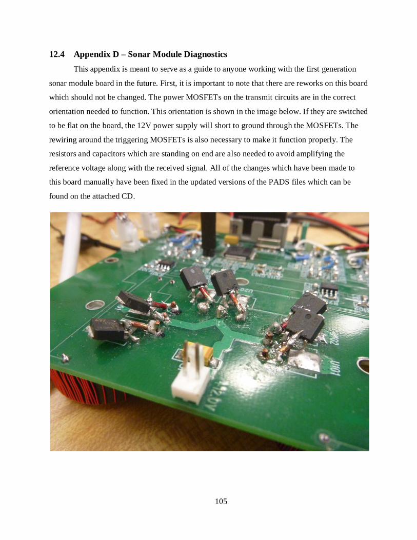
105
12.4 Appendix D – Sonar Module Diagnostics This appendix is meant to serve as a guide to anyone working with the first generation
sonar module board in the future. First, it is important to note that there are reworks on this board
which should not be changed. The power MOSFETs on the transmit circuits are in the correct
orientation needed to function. This orientation is shown in the image below. If they are switched
to be flat on the board, the 12V power supply will short to ground through the MOSFETs. The
rewiring around the triggering MOSFETs is also necessary to make it function properly. The
resistors and capacitors which are standing on end are also needed to avoid amplifying the
reference voltage along with the received signal. All of the changes which have been made to
this board manually have been fixed in the updated versions of the PADS files which can be
found on the attached CD.
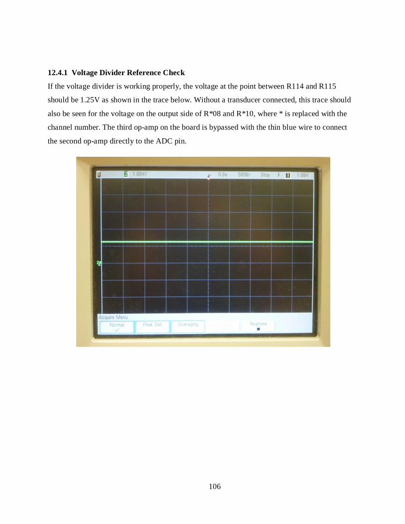
106
12.4.1 Voltage Divider Reference Check
If the voltage divider is working properly, the voltage at the point between R114 and R115
should be 1.25V as shown in the trace below. Without a transducer connected, this trace should
also be seen for the voltage on the output side of R*08 and R*10, where * is replaced with the
channel number. The third op-amp on the board is bypassed with the thin blue wire to connect
the second op-amp directly to the ADC pin.
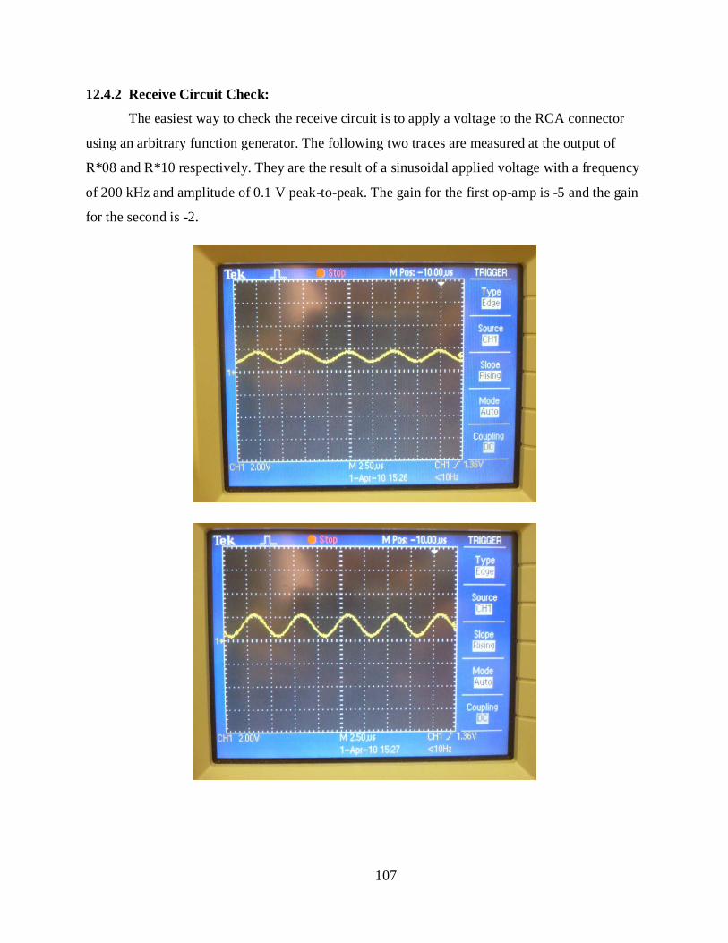
107
12.4.2 Receive Circuit Check:
The easiest way to check the receive circuit is to apply a voltage to the RCA connector
using an arbitrary function generator. The following two traces are measured at the output of
R*08 and R*10 respectively. They are the result of a sinusoidal applied voltage with a frequency
of 200 kHz and amplitude of 0.1 V peak-to-peak. The gain for the first op-amp is -5 and the gain
for the second is -2.
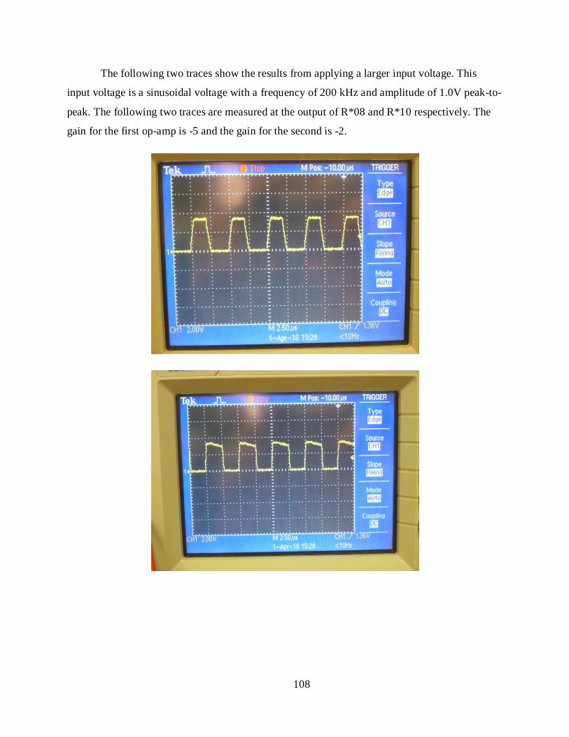
108
The following two traces show the results from applying a larger input voltage. This
input voltage is a sinusoidal voltage with a frequency of 200 kHz and amplitude of 1.0V peak-to-
peak. The following two traces are measured at the output of R*08 and R*10 respectively. The
gain for the first op-amp is -5 and the gain for the second is -2.
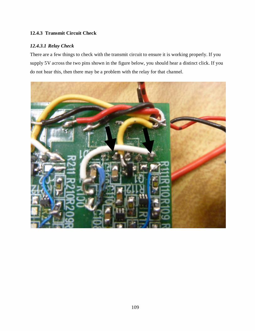
109
12.4.3 Transmit Circuit Check
12.4.3.1 Relay Check
There are a few things to check with the transmit circuit to ensure it is working properly. If you
supply 5V across the two pins shown in the figure below, you should hear a distinct click. If you
do not hear this, then there may be a problem with the relay for that channel.
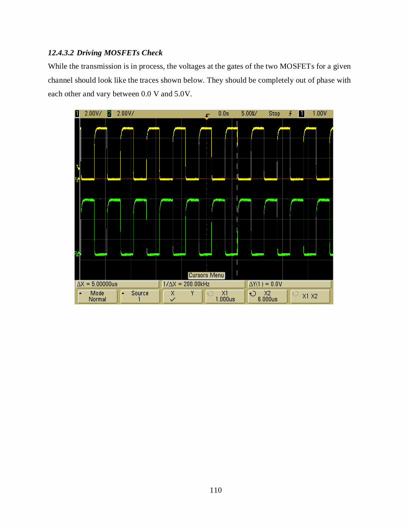
110
12.4.3.2 Driving MOSFETs Check
While the transmission is in process, the voltages at the gates of the two MOSFETs for a given
channel should look like the traces shown below. They should be completely out of phase with
each other and vary between 0.0 V and 5.0V.
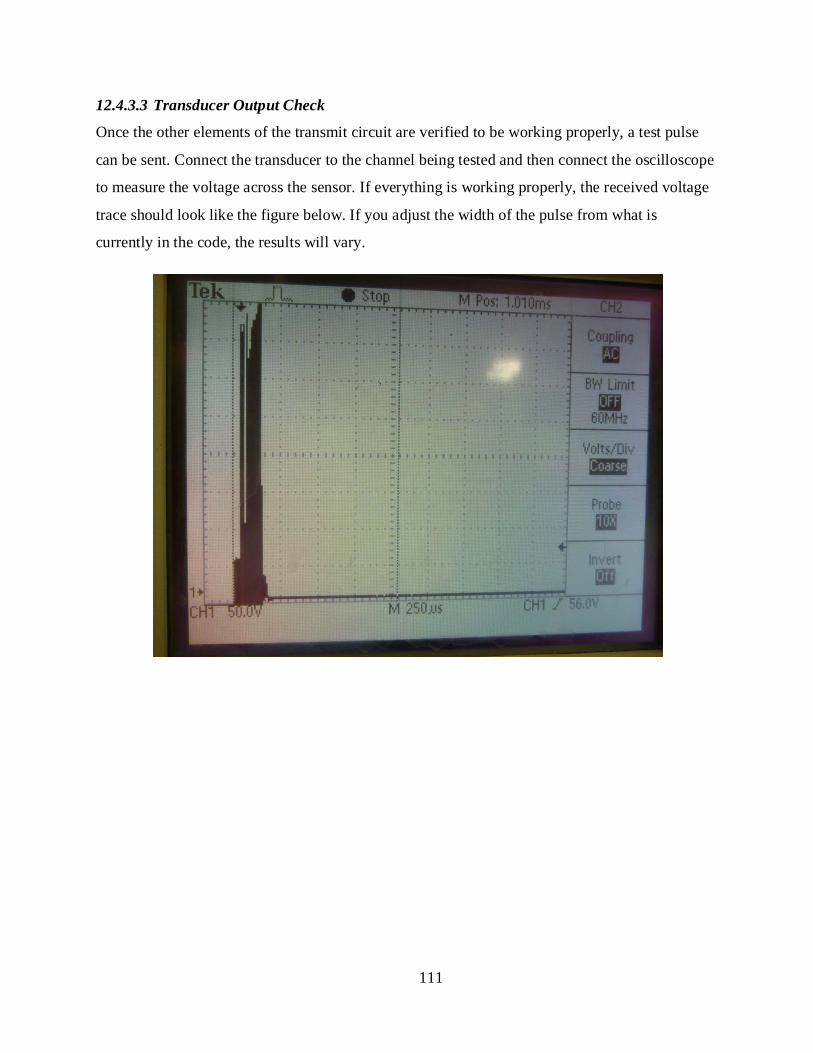
111
12.4.3.3 Transducer Output Check
Once the other elements of the transmit circuit are verified to be working properly, a test pulse
can be sent. Connect the transducer to the channel being tested and then connect the oscilloscope
to measure the voltage across the sensor. If everything is working properly, the received voltage
trace should look like the figure below. If you adjust the width of the pulse from what is
currently in the code, the results will vary.
112
12.5 Appendix E – Component Datasheets
• N-Channel 30V DPAK Power MOSFET
http://www.st.com/stonline/products/literature/ds/6763/std30nf03l.pdf
• TI MSP430F2410
http://focus.ti.com/lit/ds/symlink/msp430f2410.pdf
http://focus.ti.com/lit/ug/slau144e/slau144e.pdf
• 3V Single Supply 80 MHz High-Speed Op Amp
http://focus.ti.com/lit/ds/symlink/opa358.pdf
• 8.000 MHz Series SMD Crystal
http://www.ecsxtal.com/store/pdf/csm-7x.pdf
• DPDT Reed Relay 5VDC Open Line
http://www.reed-relays.com/files/23881270.pdf
• LM5111 Dual 5A Compound Gate Driver
http://cache.national.com/ds/LM/LM5111.pdf
• 2N7002 N Channel MOSFET
http://61.222.192.61/mccsemi/up_pdf/2N7002%28SOT-23%29.PDF
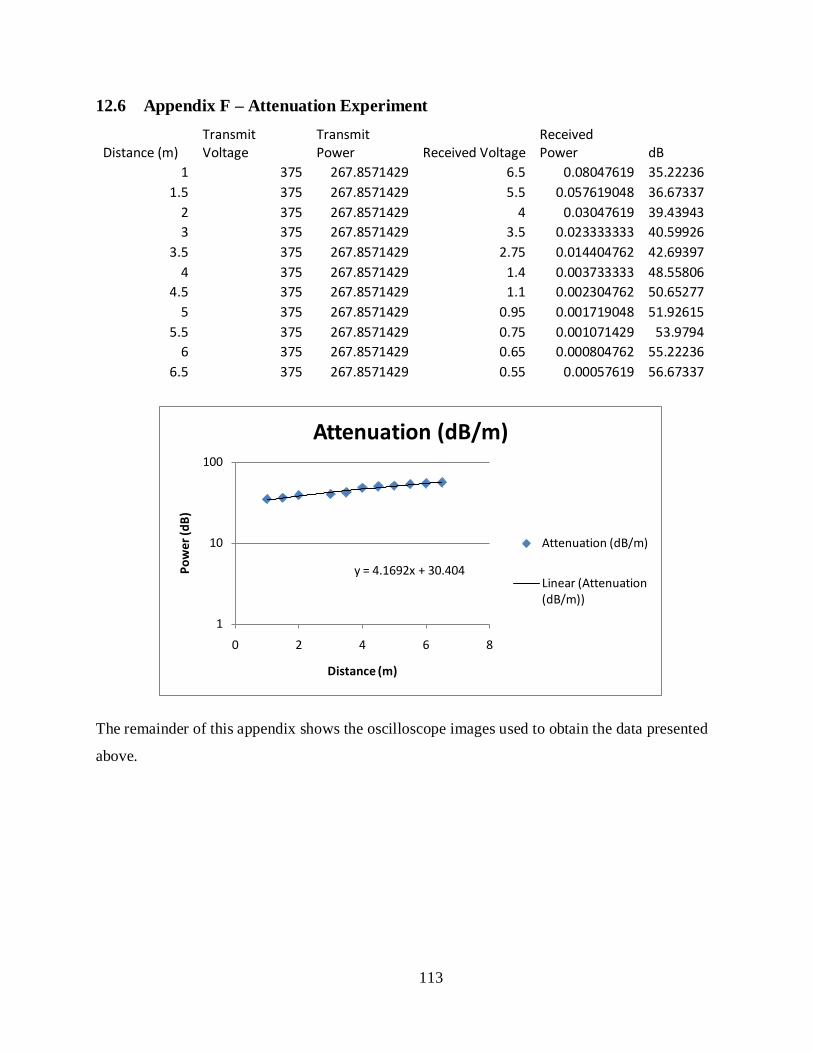
113
12.6 Appendix F – Attenuation Experiment
Distance (m) Transmit Voltage
Transmit Power Received Voltage
Received Power dB
1 375 267.8571429 6.5 0.08047619 35.22236 1.5 375 267.8571429 5.5 0.057619048 36.67337
2 375 267.8571429 4 0.03047619 39.43943 3 375 267.8571429 3.5 0.023333333 40.59926
3.5 375 267.8571429 2.75 0.014404762 42.69397 4 375 267.8571429 1.4 0.003733333 48.55806
4.5 375 267.8571429 1.1 0.002304762 50.65277 5 375 267.8571429 0.95 0.001719048 51.92615
5.5 375 267.8571429 0.75 0.001071429 53.9794 6 375 267.8571429 0.65 0.000804762 55.22236
6.5 375 267.8571429 0.55 0.00057619 56.67337
The remainder of this appendix shows the oscilloscope images used to obtain the data presented
above.
y = 4.1692x + 30.404
1
10
100
0 2 4 6 8
Pow
er (d
B)
Distance (m)
Attenuation (dB/m)
Attenuation (dB/m)
Linear (Attenuation (dB/m))
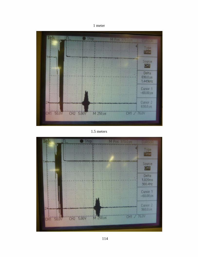
114
1 meter
1.5 meters
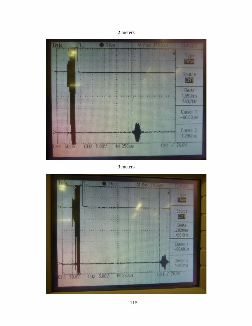
115
2 meters
3 meters
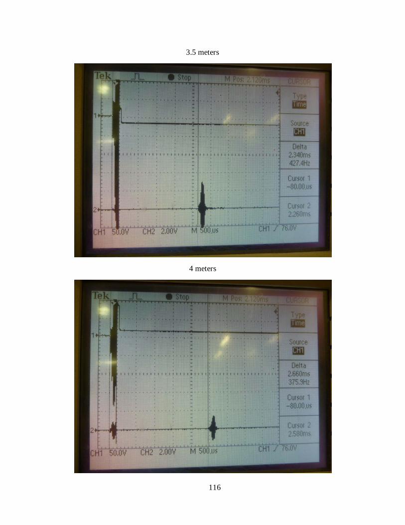
116
3.5 meters
4 meters
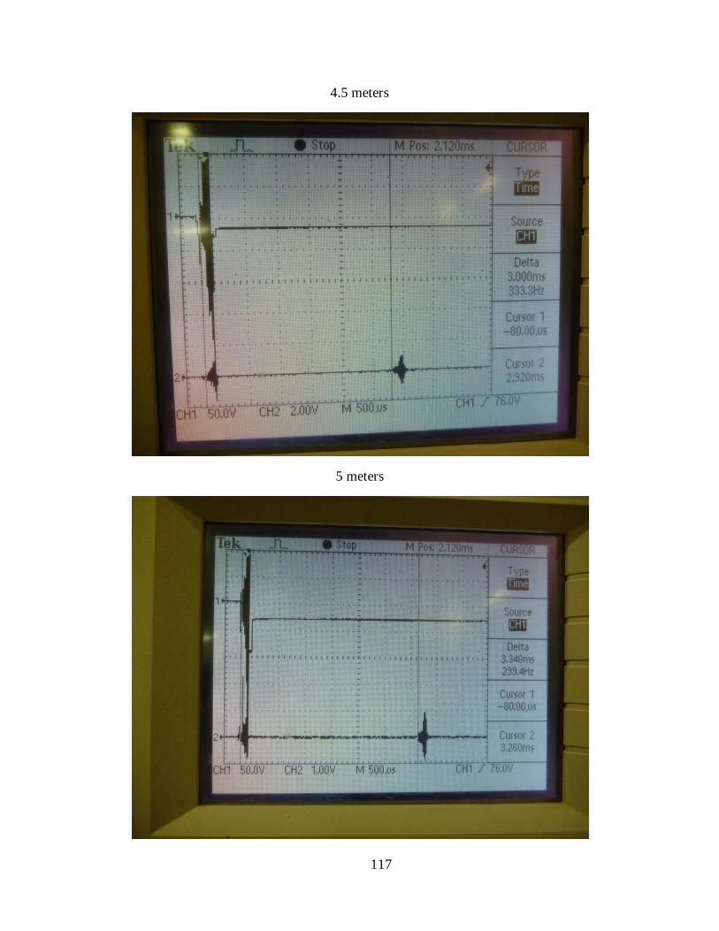
117
4.5 meters
5 meters
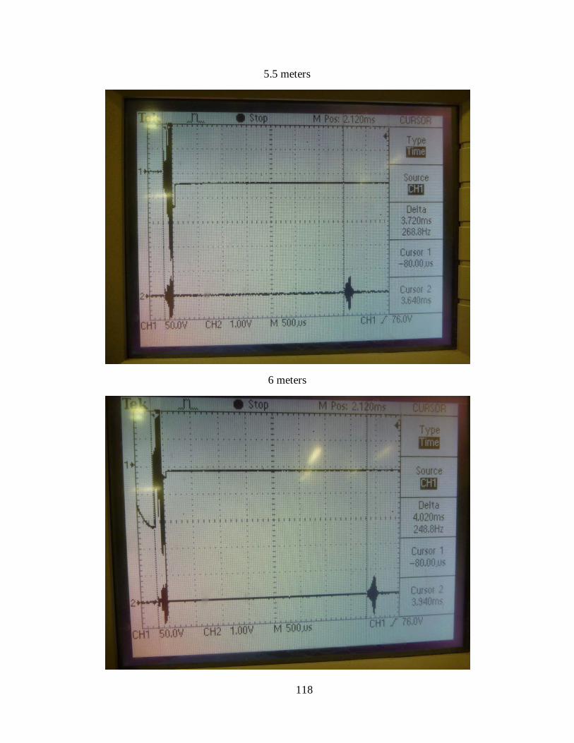
118
5.5 meters
6 meters
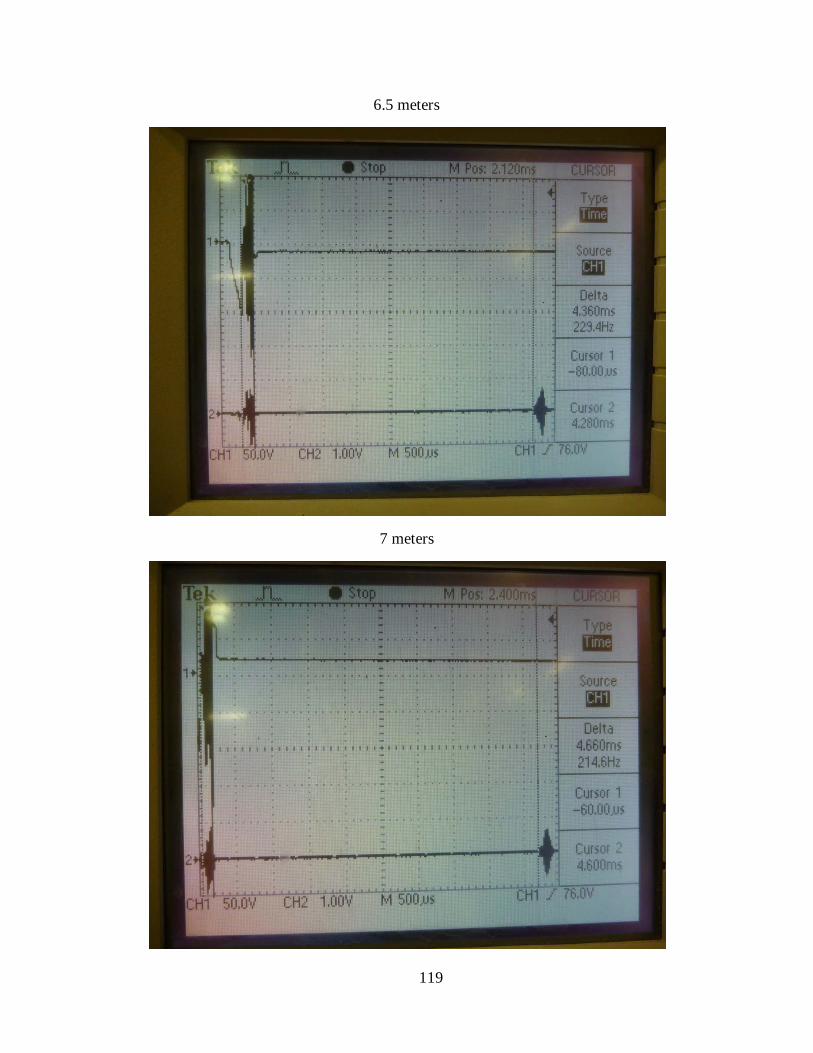
119
6.5 meters
7 meters
120
12.7 Appendix G – Threshold Determination Experiments This appendix contains the histograms used to determine the best threshold for measuring
distances with the ultrasonic sensors. It shows the experimental data gathered at a number of
thresholds. These data were used to decide on a threshold which would minimize the probability
of false detection while not increasing the probability of missed detection.
0
200
400
600
800
1000
1200
1400
1600
1800
2000
563
512
6518
9525
2531
5537
8544
1550
4556
7563
0569
3575
6581
9588
2594
5510
085
1071
511
345
1197
512
605
1323
513
865
1449
5
Freq
uenc
y
Distance measured, mm
Distance Measurement Distribution for Threshold = 1500
Threshold = 1500
121
0
200
400
600
800
1000
1200
1400
1600
1800
20005
635
1265
1895
2525
3155
3785
4415
5045
5675
6305
6935
7565
8195
8825
9455
1008
510
715
1134
511
975
1260
513
235
1386
514
495
Freq
uenc
y
Measured Distance, mm
Distance Measurement Distribution for Threshold = 1650
Threshold = 1650
0
200
400
600
800
1000
1200
1400
1600
1800
2000
563
512
6518
9525
2531
5537
8544
1550
4556
7563
0569
3575
6581
9588
2594
5510
085
1071
511
345
1197
512
605
1323
513
865
1449
5
Freq
uenc
y
Distance measured, mm
Distance Measurement Distribution for Threshold = 1800
Threshold = 1800
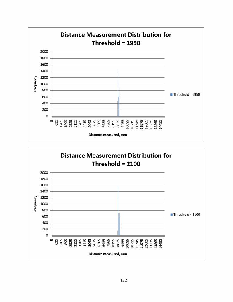
122
0
200
400
600
800
1000
1200
1400
1600
1800
20005
635
1265
1895
2525
3155
3785
4415
5045
5675
6305
6935
7565
8195
8825
9455
1008
510
715
1134
511
975
1260
513
235
1386
514
495
Freq
uenc
y
Distance measured, mm
Distance Measurement Distribution for Threshold = 1950
Threshold = 1950
0
200
400
600
800
1000
1200
1400
1600
1800
2000
563
512
6518
9525
2531
5537
8544
1550
4556
7563
0569
3575
6581
9588
2594
5510
085
1071
511
345
1197
512
605
1323
513
865
1449
5
Freq
uenc
y
Distance measured, mm
Distance Measurement Distribution for Threshold = 2100
Threshold = 2100
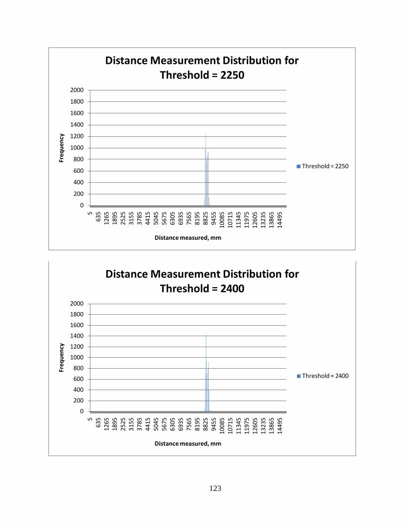
123
0
200
400
600
800
1000
1200
1400
1600
1800
20005
635
1265
1895
2525
3155
3785
4415
5045
5675
6305
6935
7565
8195
8825
9455
1008
510
715
1134
511
975
1260
513
235
1386
514
495
Freq
uenc
y
Distance measured, mm
Distance Measurement Distribution for Threshold = 2250
Threshold = 2250
0
200
400
600
800
1000
1200
1400
1600
1800
2000
563
512
6518
9525
2531
5537
8544
1550
4556
7563
0569
3575
6581
9588
2594
5510
085
1071
511
345
1197
512
605
1323
513
865
1449
5
Freq
uenc
y
Distance measured, mm
Distance Measurement Distribution for Threshold = 2400
Threshold = 2400
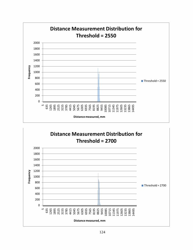
124
0
200
400
600
800
1000
1200
1400
1600
1800
20005
635
1265
1895
2525
3155
3785
4415
5045
5675
6305
6935
7565
8195
8825
9455
1008
510
715
1134
511
975
1260
513
235
1386
514
495
Freq
uenc
y
Distance measured, mm
Distance Measurement Distribution for Threshold = 2550
Threshold = 2550
0
200
400
600
800
1000
1200
1400
1600
1800
2000
563
512
6518
9525
2531
5537
8544
1550
4556
7563
0569
3575
6581
9588
2594
5510
085
1071
511
345
1197
512
605
1323
513
865
1449
5
Freq
uenc
y
Distance measured, mm
Distance Measurement Distribution for Threshold = 2700
Threshold = 2700
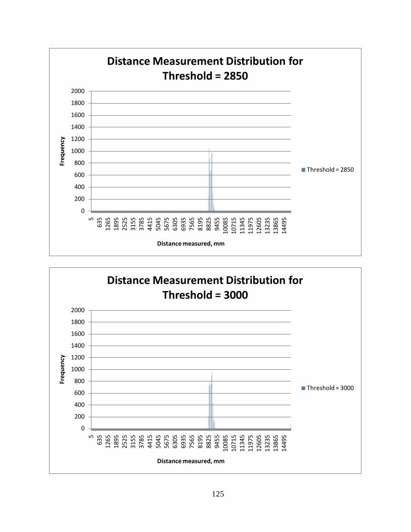
125
0
200
400
600
800
1000
1200
1400
1600
1800
20005
635
1265
1895
2525
3155
3785
4415
5045
5675
6305
6935
7565
8195
8825
9455
1008
510
715
1134
511
975
1260
513
235
1386
514
495
Freq
uenc
y
Distance measured, mm
Distance Measurement Distribution for Threshold = 2850
Threshold = 2850
0
200
400
600
800
1000
1200
1400
1600
1800
2000
563
512
6518
9525
2531
5537
8544
1550
4556
7563
0569
3575
6581
9588
2594
5510
085
1071
511
345
1197
512
605
1323
513
865
1449
5
Freq
uenc
y
Distance measured, mm
Distance Measurement Distribution for Threshold = 3000
Threshold = 3000
126
12.8 Appendix H – Localization Algorithm Mathematics This appendix shows the mathematics of the localization algorithm used for the three
orientations of the submarine which are not described in Chapter 6.
12.8.1 Orientation 2
The figures in this section are for the two determinate cases where the yaw angle is
between 90 and 180 degrees with respect to the pool coordinate system.
𝑥𝑥 = 𝑥𝑥𝐼𝐼𝑟𝑟𝐼𝐼 + 𝑑𝑑2 sin(𝜃𝜃)
𝑠𝑠 = 𝑠𝑠𝐼𝐼𝑟𝑟𝐼𝐼 + 𝑑𝑑1 sin(𝜃𝜃)
𝑃𝑃1𝑥𝑥 = 𝑥𝑥𝐼𝐼𝑟𝑟𝐼𝐼
𝑃𝑃1𝑠𝑠 = 𝑠𝑠𝐼𝐼𝑟𝑟𝐼𝐼 + 𝑑𝑑1 sin(𝜃𝜃)− 𝑑𝑑2 cos(𝜃𝜃)
𝑃𝑃2𝑥𝑥 = 𝑥𝑥𝐼𝐼𝑟𝑟𝐼𝐼 + 𝑑𝑑2 sin(𝜃𝜃) + 𝑑𝑑1 cos(𝜃𝜃)
𝑃𝑃2𝑠𝑠 = 𝑠𝑠𝐼𝐼𝑟𝑟𝐼𝐼
127
𝑥𝑥 = 𝑥𝑥𝐼𝐼𝑟𝑟𝐼𝐼 − 𝑑𝑑1 cos(𝜃𝜃)
𝑠𝑠 = 𝑠𝑠𝐼𝐼𝑊𝑊𝑥𝑥 + 𝑑𝑑2cos(𝜃𝜃)
𝑃𝑃1𝑥𝑥 = 𝑥𝑥𝐼𝐼𝑟𝑟𝐼𝐼 − 𝑑𝑑1 cos(𝜃𝜃) − 𝑑𝑑2 sin(𝜃𝜃)
𝑃𝑃1𝑠𝑠 = 𝑠𝑠𝐼𝐼𝑊𝑊𝑥𝑥
𝑃𝑃2𝑥𝑥 = 𝑥𝑥𝐼𝐼𝑟𝑟𝐼𝐼
𝑃𝑃2𝑠𝑠 = 𝑠𝑠𝐼𝐼𝑊𝑊𝑥𝑥 + 𝑑𝑑2 cos(𝜃𝜃) − 𝑑𝑑1sin(𝜃𝜃)
128
12.8.2 Orientation 3
The figures in this section are for the two determinate cases where the yaw angle is
between 180 and 270 degrees with respect to the pool coordinate system.
𝑥𝑥 = 𝑥𝑥𝐼𝐼𝑟𝑟𝐼𝐼 − 𝑑𝑑1 cos(𝜃𝜃)
𝑠𝑠 = 𝑠𝑠𝐼𝐼𝑊𝑊𝑥𝑥 + 𝑑𝑑2 cos(𝜃𝜃)
𝑃𝑃1𝑥𝑥 = 𝑥𝑥𝐼𝐼𝑟𝑟𝐼𝐼 − 𝑑𝑑1 cos(𝜃𝜃) − 𝑑𝑑2 sin(𝜃𝜃)
𝑃𝑃1𝑠𝑠 = 𝑠𝑠𝐼𝐼𝑊𝑊𝑥𝑥
𝑃𝑃2𝑥𝑥 = 𝑥𝑥𝐼𝐼𝑟𝑟𝐼𝐼
𝑃𝑃2𝑠𝑠 = 𝑠𝑠𝐼𝐼𝑊𝑊𝑥𝑥 + 𝑑𝑑2 cos(𝜃𝜃) − 𝑑𝑑1sin(𝜃𝜃)
129
𝑥𝑥 = 𝑥𝑥𝐼𝐼𝑊𝑊𝑥𝑥 + 𝑑𝑑2 sin(𝜃𝜃)
𝑠𝑠 = 𝑠𝑠𝐼𝐼𝑊𝑊𝑥𝑥 + 𝑑𝑑1sin(𝜃𝜃)
𝑃𝑃1𝑥𝑥 = 𝑥𝑥𝐼𝐼𝑊𝑊𝑥𝑥
𝑃𝑃1𝑠𝑠 = 𝑠𝑠𝐼𝐼𝑊𝑊𝑥𝑥 + 𝑑𝑑1 sin(𝜃𝜃)− 𝑑𝑑2 cos(𝜃𝜃)
𝑃𝑃2𝑥𝑥 = 𝑥𝑥𝐼𝐼𝑊𝑊𝑥𝑥 + 𝑑𝑑2 sin(𝜃𝜃) + 𝑑𝑑1 cos(𝜃𝜃)
𝑃𝑃2𝑠𝑠 = 𝑠𝑠𝐼𝐼𝑊𝑊𝑥𝑥
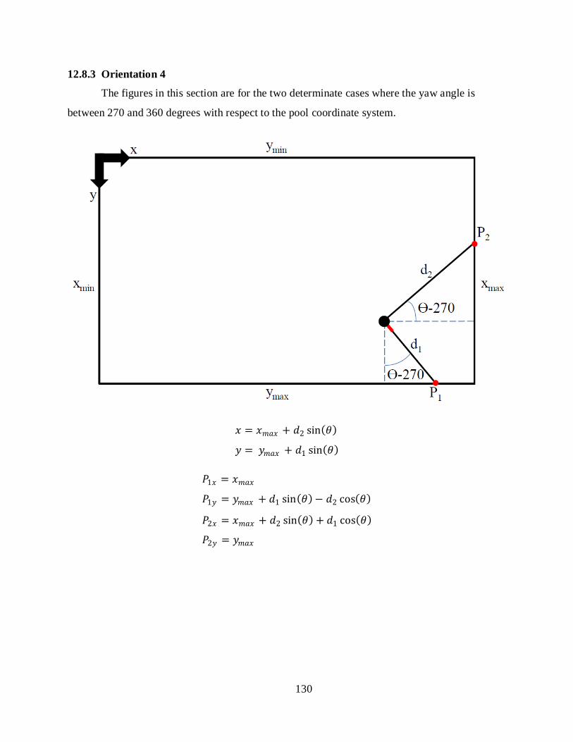
130
12.8.3 Orientation 4
The figures in this section are for the two determinate cases where the yaw angle is
between 270 and 360 degrees with respect to the pool coordinate system.
𝑥𝑥 = 𝑥𝑥𝐼𝐼𝑊𝑊𝑥𝑥 + 𝑑𝑑2 sin(𝜃𝜃)
𝑠𝑠 = 𝑠𝑠𝐼𝐼𝑊𝑊𝑥𝑥 + 𝑑𝑑1 sin(𝜃𝜃)
𝑃𝑃1𝑥𝑥 = 𝑥𝑥𝐼𝐼𝑊𝑊𝑥𝑥
𝑃𝑃1𝑠𝑠 = 𝑠𝑠𝐼𝐼𝑊𝑊𝑥𝑥 + 𝑑𝑑1 sin(𝜃𝜃)− 𝑑𝑑2 cos(𝜃𝜃)
𝑃𝑃2𝑥𝑥 = 𝑥𝑥𝐼𝐼𝑊𝑊𝑥𝑥 + 𝑑𝑑2 sin(𝜃𝜃) + 𝑑𝑑1 cos(𝜃𝜃)
𝑃𝑃2𝑠𝑠 = 𝑠𝑠𝐼𝐼𝑊𝑊𝑥𝑥
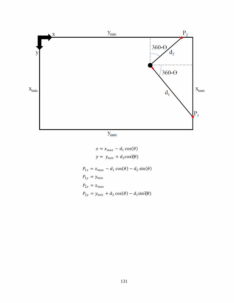
131
𝑥𝑥 = 𝑥𝑥𝐼𝐼𝑊𝑊𝑥𝑥 − 𝑑𝑑1 cos(𝜃𝜃)
𝑠𝑠 = 𝑠𝑠𝐼𝐼𝑟𝑟𝐼𝐼 + 𝑑𝑑2cos(𝜃𝜃)
𝑃𝑃1𝑥𝑥 = 𝑥𝑥𝐼𝐼𝑊𝑊𝑥𝑥 − 𝑑𝑑1 cos(𝜃𝜃) − 𝑑𝑑2 sin(𝜃𝜃)
𝑃𝑃1𝑠𝑠 = 𝑠𝑠𝐼𝐼𝑟𝑟𝐼𝐼
𝑃𝑃2𝑥𝑥 = 𝑥𝑥𝐼𝐼𝑊𝑊𝑥𝑥
𝑃𝑃2𝑠𝑠 = 𝑠𝑠𝐼𝐼𝑟𝑟𝐼𝐼 + 𝑑𝑑2 cos(𝜃𝜃)− 𝑑𝑑1sin(𝜃𝜃)

132
12.9 Appendix I – Software Explanations This appendix gives a description of software programs written for the sonar module. It is
meant to serve as a guide for anyone trying to use the programs in the future. All of the files
described here are in the folder MSP430 Code\ on the attached CD.
12.9.1 AutoTransceive2
This program transmits a signal and automatically calculates a distance from the received
signal. The program begins by initializing all the necessary registers. It is important to manually
reset the ADC so errors do not occur. Next, it sets the clock speeds and enables interrupts.
Currently, the program is configured to only work with Channel 1. It can easily be extended to
work with the other channels. Timer A is used to time the 200 kHz pulse and Timer B is used to
time the length of the pulse.
The StartPulse command is called between the two timers so the ADC will not be on too
early. If it is on early it will read the transmitted pulse instead of the received echo. The ADC is
turned on at the end of the Timer B interrupt handler. The ADC interrupt handler is where all the
filtering takes place. Only enough data for the filtering is stored in memory. Once the running
total passes the threshold, the ADC is stopped and the distance is calculated. This program
doesn’t actually do anything with the distance, so a breakpoint can be added at the distance line
to read it.
12.9.2 GetDataBack
This program is used to get data from the sonar board over a USB port using the ez430
board. You might need to reconfigure the serial port to make it work. This program should be
run after the data has been stored on the sonar board. A program such as RealTerm should be
used in conjunction with this program to capture the data as it is sent from the serial port.
When this program is run, first be sure that the sonar module has finished gathering data.
The data stream is initiated by sending a single character over the serial port. With RealTerm
open and configured properly to capture data, press any key and it will begin the data transfer.
Once the transfer stops, the data file can be saved and processed with the DataParser.py program.

133
12.9.3 Receive
This program will receive data for a given number of ADC cycles and store it in the
MSP430's RAM. This data can be retrieved with GetDataBack once it has been stored.
First, the program manually resets the ADC to avoid any problems. Next, the clock
speeds and I2C registers are set. Currently, the program is configured to receive on channel 1, but
there are functions within the program for the other two channels. The program will sample the
channel at the rate of 15.42 kHz until it reaches the preset number of data points.
12.9.4 Transceive
This program will transmit a pulse and receive data for a given number of ADC cycles.
This data is filtered and stored in the MSP430's RAM and can be retrieved with GetDataBack.
The Transceive program is similar to the AutoTransceive2 program described in Section
12.9.1. The main difference is that instead of filtering the data and calculating the distance, this
program stores the raw data in RAM to be sent to the PC later for analysis.
12.9.5 TransceiveDataCollect
This program is a modified version of AutoTransceive2 which will collect a given
number of distance measurements and store them in the RAM. Essentially, the program runs
AutoTransceive2, stores the calculated distance, and repeats this process a given number of
times. It is useful to collect a large amount of data in a short period of time. These data can be
retrieved with GetDataBack.
12.9.6 Transmit
This program transmits a single pulse on one ultrasonic axis. It is currently configured to
control the first channel, but it can easily be altered to run on the other channels. Timer A
controls the 200 kHz pulse and Timer B controls the width of the pulse. With the transceive
programs working, this program is not used too often.
12.9.7 Transmit Beacon
This program will periodically transmit a pulse on one ultrasonic axis. It is a modified
version of the Transmit program which uses Timer B to control the width of the pulse and how
often it is on or off. This program is useful for testing the receive program or for data collection.
134
12.10 Appendix J – Attached Files The following is a list of the files which can be found on the CD attached to this document.
Component Datasheets
Airmar 200A.pdf
Airmar 200BB.pdf
Airmar P23 specs.pdf
Airmar P23 wiring.pdf
DPDT Reed Relay.pdf
High Speed Op Amp.pdf
LM5111 Dual Compound Gate Driver.pdf
MSP430F2410.pdf
MSP430x2xx Family User Guide.pdf
SMD Quartz Crystal.pdf
SOT-23 N-Channel MOSFET.pdf
STD30NF03L.pdf
Documents
Thesis.pdf – A PDF version of this document.
RWM_MSThesis_032410.pdf – GRAD 2010 Poster.
SonarBoardSchematics.pdf – A PDF version of the sonar module schematics.
Excel Files
DigikeyOrder.xlsx – Lists of the parts ordered from Digikey for the board.
FilteredNoise.xlsx – A histogram of the noise distribution without filtering.
LocalizationTesting.xlsx – The raw data for the localization testing
PoolProfile.xlsx – The raw measurements for the pool depth profile
Submarine Sonar Cost Breakdown.xlsx – Detailed cost breakdown of the module.
ThresholdDetermination.xlsx – Raw data used to determine the threshold.
135
MATLAB Files
FIR.m – A simple MATLAB script to test an FIR low-pass filter.
LPF_FIR.fda – A file generated with the MATLAB Filter Design and Analysis Toolbox which describes the low pass filter for this module.
MSP430 Code
Code Explanation Key.txt
AutoTransceive2 - This program transmits a signal and automatically calculates a distance from the received signal.
GetDataBack - This program is used to get data from the sonar board over a USB port using the ez430 board. You might need to reconfigure the serial port to make it work. This program should be run after the data has been stored on the sonar board.
Receive - This program will receive data for a given number of ADC cycles and store it in the MSP430's RAM. These data can be retrieved with GetDataBack.
Transceive - This program will transmit a pulse and receive data for a given number of ADC cycles. These data is filtered and stored in the MSP430's RAM and can be retrieved with GetDataBack.
TransceiveDataCollect - This program is a modified version of Transceive2 which will collect a given number of distance measurements and store them in the RAM. These data can be retrieved with GetDataBack.
Transmit - This program transmits a single pulse on one ultrasonic axis.
TransmitBeacon - This program will periodically transmit a pulse on one ultrasonic axis.
PADS Files
ultrasonic_032510.pcb – Printed circuit board layout files from PADS
ultrasonic_032510.sch – Schematics files from PADS
Russ Library
Radu Library
MAX Library
ProEngineer Files
frame_assembly.asm.1
h-channel.prt.1
hull_bottomdefault_as_machined_.prt.2
136
hull_top.prt.2
mountflange.prt.16
sonarsensor.asm.14
sonarsensorbody.prt.33
spool.prt.2
spooltop.prt.2
submarine.asm.3
submarine_assembly.asm.1
transducer.prt.13
transducerasis.prt.2
Python Files
Code Explanation Key.txt
Data Parser - This program is used in conjunction with the data stored from the GetDataBack program. It is needed to convert the data from hexadecimal format back to 16 bit integers so they can be processed.
Localization Simulation - This program is a graphical simulation of the 2D portion of the localization algorithm. The position and orientation of the submarine can be changed manually and the program calculates the position using the algorithm. If a coordinate is indeterminate, the value is listed as 0.
Visio Files
3DLocalizationFlowChart.vsd – A flow chart showing the process for 3D localization.
BlockDiagramSignalProcessing.vsd – A block diagram showing the general layout of the localization module.