Acta Cryst. (2014). A70, 257–282 doi:10.1107/S205327331400117X 257

research papers

Acta Crystallographica Section A

Foundations andAdvances

ISSN 2053-2733

Received 1 August 2013

Accepted 16 January 2014

A new theory for X-ray diffraction

Paul F. Fewster

PANalytical Research Centre, Sussex Innovation Centre, Falmer, Brighton, East Sussex BN1 9SB,

UK. Correspondence e-mail: paul.fewster@panalytical.com

This article proposes a new theory of X-ray scattering that has particular

relevance to powder diffraction. The underlying concept of this theory is that the

scattering from a crystal or crystallite is distributed throughout space: this leads

to the effect that enhanced scatter can be observed at the ‘Bragg position’ even

if the ‘Bragg condition’ is not satisfied. The scatter from a single crystal or

crystallite, in any fixed orientation, has the fascinating property of contributing

simultaneously to many ‘Bragg positions’. It also explains why diffraction peaks

are obtained from samples with very few crystallites, which cannot be explained

with the conventional theory. The intensity ratios for an Si powder sample are

predicted with greater accuracy and the temperature factors are more realistic.

Another consequence is that this new theory predicts a reliability in the intensity

measurements which agrees much more closely with experimental observations

compared to conventional theory that is based on ‘Bragg-type’ scatter. The role

of dynamical effects (extinction etc.) is discussed and how they are suppressed

with diffuse scattering. An alternative explanation for the Lorentz factor is

presented that is more general and based on the capture volume in diffraction

space. This theory, when applied to the scattering from powders, will evaluate

the full scattering profile, including peak widths and the ‘background’. The

theory should provide an increased understanding of the reliability of powder

diffraction measurements, and may also have wider implications for the analysis

of powder diffraction data, by increasing the accuracy of intensities predicted

from structural models.

1. Introduction

The concept of Bragg’s law assumes that the scattering is

concentrated at discrete points and that away from these

positions the mutual interference gives no significant scat-

tering (Bragg, 1925). An alternative viewpoint is presented

here, where the whole of diffraction space is occupied by

scattering from many crystal planes, which when combined

contribute to the peaks observed. This effect is most obvious

in X-ray powder diffraction and this is therefore the main

focus of this article.

X-ray powder diffraction was pioneered by Debye &

Scherrer (1916) and is now a well established technique that

has been used successfully for nearly 100 years. This is a very

important technique for the identification of material phases

and their quantitative proportion, microstructure evaluation

and molecular structure determination. A powder is in general

an accumulation of small crystallites with dimensions �10 mm

or less. Most materials have some identifiable atomic peri-

odicity and therefore create an X-ray diffraction pattern. This

gives X-ray powder diffraction an important role in many

industries from building materials, pharmaceuticals, mining,

forensic analysis etc., to scientific studies on the evaluation of

the microstructure and the determination of the stereo-

chemistry of molecular structures. These analyses give infor-

mation on the strength of materials, liability to cracking in

structures, identification of polymorphs in drug design, iden-

tification of phases and their proportions in paints and cement

etc. Its impact worldwide has been enormous and many

important processes depend on X-ray powder diffraction.

However, the ‘standard explanation’ of the diffraction process

raises some concerns: for example, the low probability of

Bragg scattering (Fewster, 2000), the high variability in peak

shapes depending on experimental procedure (Fewster &

Andrew, 1999) and the poor reliability of intensity measure-

ment based on crystal statistics (Smith, 1999). Despite these

concerns, the method seems to work. It is the position, width

and intensity of the diffraction peaks that yield the informa-

tion for the analyses mentioned above.

This article will give a brief outline of the conventional

theory of X-ray powder diffraction and its shortcomings,

including the theoretical estimates of crystal statistics and

estimates of temperature factors, followed by an alternative

theory that addresses these weaknesses. Attention will be

drawn to the relevance of dynamical and kinematical scat-

tering and the origin of the intensity, the improvement in the

intensity estimates when compared with measured values and

the complex nature of the intensity distribution. The whole

process, based on this alternative theory, is much more subtle

and fascinating than can be explained by the simple applica-

tion of Bragg’s law. This improved understanding has led to,

and may in the future lead to further, new diffractometer

designs, more robust analyses of the data and a firmer basis for

establishing the reliability of the method.

2. The conventional theory

The expression for the diffracted intensity from powders has

been presented by several authors and has the form given by

I2� / I0Mhkl Fhkl

�� ��2 1þ cos22�Bcos22�m

2

� �1

sin 2�B sin �B

� �:

ð1Þ

This expression can be derived based on a flat-plate detector

set normal to the incident beam after passing through a small

cluster of crystallites, e.g. Zachariasen (1945), and also is given

by James (1962) for the basic single-crystal diffraction process,

and by Brown (1955) for a cluster of crystallites as in the case

discussed. The constant of proportionality includes absorp-

tion, wavelength effects, specimen-to-detector radius, classical

electron radius etc., which are all constant in a typical X-ray

diffraction experiment. In the above equation, I0 is the inci-

dent-beam intensity, �B and �m are the Bragg angles for the

sample and the monochromator crystal, if one exists, respec-

tively, and Mhkl is the multiplicity (the number of times a

similar reflection occurs by symmetry). Fhkl is the structure

factor and is the coherent sum of the scattering fr from all the

atoms, located at fractional coordinates xi, yi, zi in the unit cell

repeat through the structure; it is given by

Fhkl ¼

Zr

fr exp �Bsin �

�

� �2" #

exp �2�iSrð Þ dr

�X

r

fr exp �Bsin �

�

� �2" #

exp �2�iSrð Þ; ð2Þ

where r = hxj + kyj + lzj, |S| = 2 sin �/�, B is the Debye–Waller

factor (Debye, 1913; Waller, 1923) and � is the wavelength.

The first bracketed term in equation (1) takes account of the

reduction in the intensity of one of the polarization compo-

nents (� polarization) in the plane of the scattering, and the

second term is a combination of the Lorentz factor and a

geometric factor. The Lorentz factor is expressed as the time

for the reflection to stay in the ‘Bragg condition’, and one of

the first texts to discuss this was by Debye (1913) and a

detailed derivation was given in Buerger (1940). Based on this

description it is not applicable to any arbitrary position in

diffraction space, but only at the ‘Bragg condition’. This term

can be expressed as 1/sin 2�B. The geometric term, 1/sin �B, is

related to the range of crystal plane tilts that will give rise to

measured scattering through a fixed detector aperture (this

can be visualized by recognizing that a large crystal plane tilt is

required to rotate the scattered beam across the detector

aperture at low scattering angles).

The intensity formula, equation (1), contains no informa-

tion about the peak widths and is considered as the intensity

associated with the ‘Bragg condition’. The peak shapes are

superimposed on this ‘stick pattern’ to smear the intensity and

form the profiles for comparison with the measured profiles.

The peak shapes are often considered as a fitted parameter

containing some mixture based on Lorentzian and Gaussian

forms, e.g. Pearson VII, pseudo-Voigt (see, for example,

Young, 1993). The peak widths are usually fitted to a quadratic

tangent function (Caglioti et al., 1958) which represents the

varying instrument function over the experimental scan angle.

The Caglioti function was derived for neutron diffractometry,

assuming Gaussian profiles, and does not include the full

instrument response. These functions do not account for the

intensities between the peaks, unless more parameters are

included that can be attributed to the sample.

The same formula, equation (1), is used for Bragg–

Brentano focusing geometry as well as the Debye–Scherrer

geometry; however, this does use an assumption that alters the

relative intensities for the two geometries, but it is a small

effect. The validity of this assumption is discussed later. The

whole expression relies on a considerable degree of averaging

and assumes that the diffraction profile comes purely from the

crystallites that are in the Bragg condition (Bragg, 1913, 1925).

3. The problem with conventional theory

The conventional theory of X-ray powder diffraction is based

on the scattering at the Bragg condition for each crystalline

plane, and assumes that there are sufficient crystallites in the

correct orientation to create the pattern observed. At first

sight this seems reasonable, since generally there could be

millions of crystallites illuminated at any one time using

standard instrumentation. This assumption will be considered

in more detail. The geometry of the instrument along with the

crystallite orientation distribution will give an estimate of the

intensities for the scattering peaks.

The conventional understanding of powder diffraction will

be considered in terms of:

(i) the likelihood of scattering at the Bragg condition,

(ii) the influence of sample movement,

(iii) the influence of dynamical and kinematical scattering,

(iv) the estimation of the temperature factors,

(v) an experiment illustrating the serious deficiency of

conventional theory.

These aspects will be considered briefly at this stage with an

emphasis on some experimental pointers and then be

considered in detail later in the article.

3.1. The likelihood of scattering in the Bragg condition

If we consider two well characterized sample types, Si and

LaB6 used in this study, it is possible to estimate the chance of

scattering in the Bragg condition with the conventional

Bragg–Brentano diffractometer (Bragg, 1921; Brentano,

1946). The geometry of the Bragg–Brentano diffractometer is

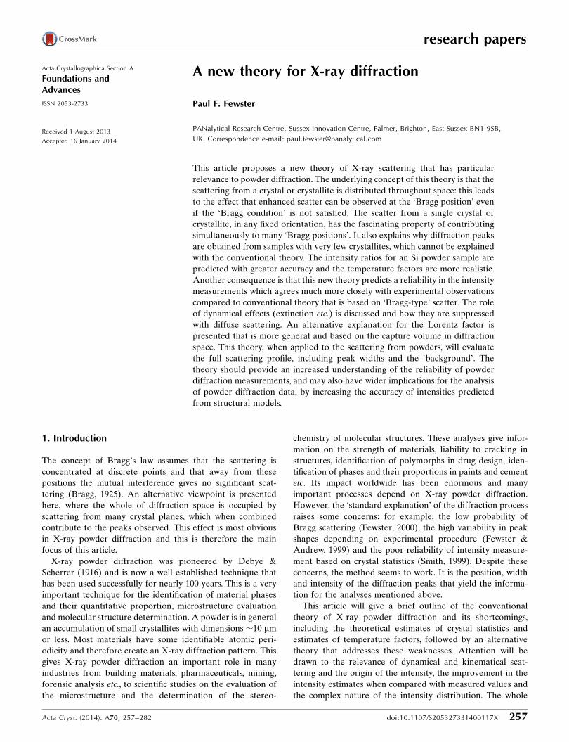
given in Fig. 1(a). With this para-focusing geometry the sample

research papers

258 Paul F. Fewster � A new theory for X-ray diffraction Acta Cryst. (2014). A70, 257–282

area illuminated can be very large. A typical instrument

source-to-sample distance is 240 mm with a beam width of

10 mm. Within the plane of the diffractometer, the X-ray

source focus dimension could be typically 40 mm, with the

divergence slit set at 0.25� and the acceptance slit at 0.25�.

Alternatively, the area illuminated could be fixed at 10 �

10 mm. An approximate calculation is performed for both

configurations.

The Si sample is composed of 10 mm perfect crystalline

spheres and most of the scattering comes from the top 30 mm.

The absorption length for Si is �63 mm, then for a perfectly

packed sample the total number of crystallites illuminated by

the incident beam would be �2 406 000 at 15� 2�, �1 212 000

at 30� 2�, falling to �618 000 at 60� 2�. For a fixed incident-

beam area the number of illuminated crystallites is 3 000 000

at all angles. For LaB6 the absorption length is �1 mm and the

crystallite dimension is 3 mm. Therefore the numbers of crys-

tallites illuminated are �8 880 000 at 15� 2�, �4 470 000 at 30�

2�, falling to �2 310 000 at 60� 2�, assuming that the pene-

tration is not greater than 3 mm. For a fixed area of 10 �

10 mm, the number of crystallites illuminated is 11 100 000. In

practice, though, these are overestimates, but give a working

value to illustrate the problem with the conventional theory.

These values also assume that there is no loss of intensity

through scattering; these are extinction effects incorporated

into dynamical theory and could reduce the absorption depth

further, and this would vary with reflecting power.

If the scattering from an individual crystallite is considered,

then the divergence it experiences is calculated from the

geometry of Fig. 1(a), for the scattering normal to the

diffractometer axis. For a 10 mm crystallite, 40 mm focus and a

radius of 240 mm the accepted divergence is 0.017� and for a

3 mm crystallite this is 0.01�. In the plane normal to Fig. 1(a),

given in Fig. 1(b), there will also be some axial divergence that

is restricted by Soller slits; for this example a typical diver-

gence control could be based on 0.04 radian Soller slits. The

axial divergence parallel to the diffractometer axis is defined

by the Soller slit (or the detector dimension) geometry in Fig.

1(b). The probability of this geometry capturing scatter that

satisfies the Bragg condition, for a specific reflection from one

crystallite, is given by the product of these orthogonal

accepted divergences by the crystallite compared to 4�. This

can be visualized as the small acceptance region on the surface

of a sphere representing the distribution of orientations

compared to that of the whole sphere surface. Therefore for

the geometry in Fig. 1 the number of crystallites, X, that are

involved in contributing to the intensity through Bragg scat-

tering for a sample with N (= 2 406 000, 1 212 000 and 618 000

at 15�, 30� and 60� 2�) 10 mm Si crystallites is approximately

X ¼0:017 �

180

� �0:04

4� sin �N ¼

9:44� 10�7

sin �N ’ 17! 4:4! 1:1

ð3aÞ

(� = 15� ! 30� ! 60�). And for 3 mm closely packed LaB6

crystallites

X ¼0:01 �

180

� �0:04

4� sin �N ¼

5:55� 10�7

sin �N ’ 37! 9:6! 2:5

ð3bÞ

(� = 15� ! 30� ! 60�). Therefore with this large number of

crystallites, on average there will be very few that satisfy the

Bragg condition for any specific reflection. The 1/sin � equates

to the 1/sin �B term in equation (1). The counting statistics

would be very poor, and going to high angular resolution

instruments this would create very unreliable data. Smith

(1999) estimated the unreliability in the data and concluded

that any accurate analysis of minor phases in a mixture would

be impossible, but was assuming thousands of millions of

crystallites were contributing. However, the intensities are

reproducible, which is difficult to reconcile with the assertion

that the scattering only comes from the ‘Bragg condition’. To

account for this apparent reliability, Alexander et al. (1948)

had to assume that the crystallites were quite imperfect and

had to diffract over considerably wider angles than their

expected perfect width, whereas de Wolf (1958) assumed that

the instrumental broadening was a significant contributor.

Any single crystallite will have many hundreds of possible

reflections. Take for example the standard reference material

LaB6, a cubic structure, which has 690 possible reflections

accessible with Cu K�1 radiation. The number of observable

diffraction peaks is 25; due to symmetry, however, it must be

assumed that a significant number of reflections contribute to

the 25 2� positions to obtain reproducible intensity ratios. This

still puts great demands on the range of crystallite orienta-

tions, despite having a small lattice parameter and therefore

few possible reflections. For more complex structures, with

lower symmetry and many thousands of reflections, the

number of crystallites required to satisfy the Bragg condition

for all the possible reflections, based on the conventional

theory, will become very large or the intensities would be very

unreliable.

Acta Cryst. (2014). A70, 257–282 Paul F. Fewster � A new theory for X-ray diffraction 259

research papers

Figure 1(a) The Bragg–Brentano geometry with a sample including crystallites ofdiameter L, which experience an angular spread defined by L and thefocus dimension F. (b) is the projection normal to (a). R is the radius, Sare the Soller slits that control the axial divergence, Sr is the receiving slit,D the detector and Sd the divergence slit.

3.2. The effect of sample movement

Introducing sample rotation within the beam certainly

improves the reliability in the intensities; however, a

stationary sample can still produce all the reflections in the

diffraction pattern and give very reproducible intensity ratios.

Sample rotation in the Bragg–Brentano geometry increases

the angular spread impinging on the sample, and the prob-

ability of satisfying the Bragg condition, by a very small

amount, mainly because only those crystallites with the

appropriate plane closely parallel to the surface will produce

Bragg diffraction.

3.3. The influence of dynamical and kinematical scattering

Depending on the material, there are significant differences

in the calculated intensities when using kinematical and

dynamical theories. For example, LaB6, hkl = 003, and Si, hkl =

004, both with crystallite dimensions of 3 mm will introduce a

peak intensity difference of �20% (the kinematical scattering

theory overestimates), which reduces with decreasing crys-

tallite dimensions. The stronger reflections of LaB6, e.g. hkl =

110, have considerable dynamical effects and the calculated

kinematical peak intensity is �60, for this 3 mm dimension,

compared with that calculated from dynamical theory. The

scattering from the Bragg condition must therefore be

included or reasons given as to why these dynamical effects

are suppressed. However, the intensities derived using equa-

tion (1) that is based on kinematical theory fit reasonably well,

and so an explanation for the suppression of dynamical effects

is required. Darwin (1922) considered various crystal imper-

fections to suppress the dynamical effects: the most likely

description was termed the mosaic crystal, sometimes termed

‘ideally imperfect’, which effectively consists of small blocks of

perfect crystal that have slightly different orientations with

respect to each other (Zachariasen, 1945). The size of blocks

has to be small enough to suppress dynamical effects. As

shown in the example above, the blocks need to be very small,

probably sub-micron, for kinematical theory to be valid.

The conventional theory does not in general include

refractive-index effects, although this has been discussed by

Wilson (1940) for powders, whereas dynamical theory includes

them naturally. However, the neglect of the refractive index

makes for a very small displacement of the peaks, �0.005� for

a flat plate, which is close to the maximum value at normal

incident angles and can be 0.0� for entry and exit through

surfaces normal to the scattering planes. It is debatable

therefore whether the refractive index should be included

to estimate the peak positions in powder diffraction. This

maximum displacement of the peaks is �10% of the intrinsic

scattering width of the profiles in a typical powder diffraction

experiment. Hart et al. (1988) have discussed the ratio of

transmission to reflection geometry based on scattering in the

symmetrical ‘Bragg condition’ and estimated that it is domi-

nated by transmission geometry. This would suggest that the

refraction effect would be small and cannot account for the

measured difference in lattice parameters between poly-

crystalline Si and bulk Si (Hubbard et al., 1975). Another

important conclusion of the work of Hart et al. is that the

refractive index is negligible at large extinction distances: the

extinction distance is smallest for intense Bragg reflections

that have the largest dynamical effects.

3.4. Estimation of the temperature factors in Si

Carefully collected experimental data sets for Si powder,

using Cu K�1 in para-focusing geometry, exhibit highly

reproducible intensity values and ratios; however, on applying

the intensity formula in equation (1), the relative intensities

appear slightly overestimated with increasing 2� angle (Fig. 2).

If the dynamical effects discussed in the previous section are

included then the agreement in the intensities is considerably

worse. This difference can be resolved by allowing the Debye–

Waller factor to increase, e.g. to B � 0.06 nm2, if the scattering

follows kinematical theory, and B � 0.08 nm2 if it follows

dynamical theory. This B factor is difficult to reconcile

with the expected value of �0.02 nm2 (Reid & Pirie, 1980).

The experimentally measured parameter on bulk Si of B

�0.046 nm2, by Aldred & Hart (1973), represents the

maximum value, because their experimental conditions were

highly biased towards the core value. Reid & Pirie (1980) have

critically reviewed the literature as well as having calculated

this value for Si by numerous approaches, and concluded that

B �0.02 nm2 is the most likely value. The structure of Si is

known and therefore there is little room for manoeuvre. The B

factor is not the complete description of thermal effects on the

intensities, because this relates to the averaging of uncorre-

research papers

260 Paul F. Fewster � A new theory for X-ray diffraction Acta Cryst. (2014). A70, 257–282

Figure 2The integrated intensity for the measured reflections (grey central bars)displayed as a bar graph for an Si sample (Si crystallites immersed in aresin that occupy 50% of the volume), compared with the conventionaltheory: blue right-hand bars, include dynamical effects, cyan left-handbars based purely on kinematical theory (large diamonds for B =0.02 A�2, small diamonds for B = 0.046 A�2). The experimental data werecollected on an instrument with R = 320 mm, divergence slit = 0.125�, aPIXcel detector with 255 strips of 0.055 mm and Soller slits of 0.04 radianand Cu K�. The black diamond is the mean of six measurements ondifferent samples, the ‘x’ marks are the standard deviation points and ‘o’symbols the range.

lated atomic vibrations and assumes the vibrations are

isotropic. The discussion on the Debye–Waller factor is given

in the Appendix.

3.5. An experiment illustrating a serious deficiency ofconventional theory

Suppose a sample with very few crystallites is studied: it is

expected that the chances of observing any scattering is very

unlikely, based on crystallites satisfying the ‘Bragg condition’.

However, as can be seen in Fig. 3(a), for <300 crystallites and

no sample movement, there is a very clear diffraction pattern

from LaB6, with all the possible reflections being observed in

the angular range of the experiment. With so few crystallites, a

single crystal plane (hkl) will have on average an angular

separation between different crystallites of �11�. This is

clearly outside the range of probability for capture. This

experiment used a pure Cu K�1 incident beam (3.5 mm

FWHM � 1000 mm) with an angular divergence of 0.01� and a

Soller slit acceptance of 2.3� (0.04 radian) (Fewster & Trout,

2013). The sample consisted of a single layer of crystallites; if

the crystallites covered the adhesive mounting tape used, with

no gaps, then the crystallite number would be �300. From

X-ray absorption measurements this is unlikely and �40%

coverage is typical, giving a crystallite number �120. A more

extreme example is given for a sample of �30 crystallites or

for a perfectly packed sample �75 crystallites (Fig. 3b). The

intrinsic scattering half-height width for a 3 mm crystallite is of

the order of 0.002�, which is small compared with the capture

volume and so has little influence on the capture likelihood.

This experiment will also give an estimate of the intensity

impinging on a single crystallite. The direct beam has a flux of

10 000 photons per second on a 10 mm circular cross section,

within a divergence of 0.017�. If it is assumed that the half-

height width of a scattering peak is 0.002�, then each crystallite

in the Bragg condition should scatter �1176 � R photons [=

10 000 � (0.002/0.017) � R], where R is the reflectivity.

Suppose the reflection being studied is the 220 from Si, then

from dynamical theory R � 96% for 10 mm assuming a

simplified model (for 3 mm crystallites R falls to 73%), giving

an expected intensity of 1130 photons for each Bragg condi-

tion satisfied. This expected intensity is �100� greater than

the total intensity gathered for this reflection from 22001

crystallites, assuming a 40% coverage.

In summary, the intensity is captured for all peaks and

contradicts the notion that there must be a statistically large

enough number of crystallites, for a sufficient number of

reflections to be in the ‘Bragg condition’. Furthermore if the

observed reflections satisfied the ‘Bragg condition’, then they

would be expected to be >100� more intense than they

actually are. Both these observations call into question the

idea that the reflections must satisfy the ‘Bragg condition’, i.e.

arise purely from the condition when crystallites are orien-

tated exactly for Bragg’s law to be obeyed.

4. An alternative explanation

If the whole diffraction process is considered as an inter-

ference problem then the contributions are not confined to the

Bragg condition. To describe the concept, the scattering is

treated kinematically initially, i.e. there is no inclusion of

dynamical effects, for example extinction (incident energy loss

through scattering) and refraction effects (the refractive index

of typical materials with X-rays is �0.9999).

The profile calculations based on dynamical and kinema-

tical theories are coincident remote from the Bragg condition,

when the refraction correction is ignored. The kinematical

profile at the Bragg condition is slightly asymmetric for strong

reflections when absorption is considered; however, when this

is ignored, the profile matches that of a sine cardinal (sinc

function). The sinc function is a very convenient way of

representing the scattering profile by just considering the path

differences of possible scattered beams; therefore sinc func-

tions are used to illustrate the basic concepts in this article,

although as will be shown later dynamical theory is included.

5. The derivation of the amplitudes

The amplitude A� at the point P(2�) (Fig. 4a) for a beam

incident at an angle � to a crystal plane is found by deriving

the phase difference for different possible paths, which can be

represented by a sinc function:

A� ¼sin �Lx

� cos 2� ��0ð Þ � cos �0

� � �Lx

� cos 2� ��0ð Þ � cos �0

� � : ð4Þ

The shape of this profile is a function of the scattering plane

lateral dimension in the plane of the incident-beam direction,

Acta Cryst. (2014). A70, 257–282 Paul F. Fewster � A new theory for X-ray diffraction 261

research papers

Figure 3The scattering pattern from �120 crystallites or if perfectly packed 300crystallites (3.5 mm beam width � 1 mm sample size and a single layer ofcrystallites) of LaB6 with crystallite sizes varying from 2 to 5 mm with thefull range of reflections up to 80� 2� (a). (b) gives the profile with �30crystallites or if perfectly packed 75 crystallites (3.5 mm beam width �0.25 mm sample size), where not all the reflections are clearly resolved asin the larger sample size. The data were collected with a 0.01� divergentCu K�1 beam from a 1.8 kW X-ray laboratory source and a stationarysample in 35 min.

1 The number of 5 mm radius crystallites irradiated during this experiment, bya beam of 35 mm wide and 256� 55 mm pixels = 35� 256� 55/(�52)� 40% =2509.

Lx. The position of the detector is set to detect scattering at an

angle 2� with respect to the incident beam. The maximum

reflecting power occurs at � = � and is the specular reflection

from a single plane of atoms at this incident angle. A� is the

amplitude recorded at P(2�) as the crystallite is rocked about

an axis normal to the incident and scatter beams (Fig. 4b).

Within a perfect crystal there will be many parallel planes

that scatter as above, and their amplitudes are added taking

into account their phase relationships. The maximum ampli-

tude occurs when the phase difference between the different

possible paths is zero or n�, where n is an integer, and when

the amplitude A� is at a maximum. The amplitude combina-

tion therefore falls in magnitude as � differs from �, equation

(4), and when � differs from the perfect constructive inter-

ference combination of waves, A2� . The latter amplitude is

analogous to scattering by a diffraction grating, which is the

product of the amplitude of a single slit and that from many

slits (e.g. Jenkins & White, 1957).

It is important to show that the scattering from a stack of

parallel planes remains in phase when � 6¼ �B at the scattering

angle 2�B. Fig. 4(a) shows the end point of summing a large

number of waves scattered across the surface of a plane;

however, the separation between the scattering points, x in

Fig. 4(c), makes no difference to the end result for A�

provided x is small. The trajectories A0, B0, C0 and D0 all

represent possible paths for a photon, and the combination

A0A1 and C0C1 and similarly B0B1 and D0D1 will always have

a value of x that will keep them in phase. The path difference

� for a given x is ab + bc in Fig. 4(d), where

� ¼ d sin �þ sin 2� ��ð Þ½ � � x cos �� cos 2� ��ð Þ½ �

where x can be determined by equating � = 2dsin � which is

the condition when x = 0, and must also be satisfied; therefore

x ¼ dsin �þ sin 2� ��ð Þ � 2 sin �

cos �� cos 2� ��ð Þ:

The values of x/d vary from 0 to a maximum of typically �0.1

(for a Bragg angle of 14.2� and 0 < � < 28.4�), the phase is only

maintained provided x < the crystallite dimension or the

coherence length. This path difference leads to the amplitude

for a stack of parallel planes being

A�2� ¼ A�A2�

¼sin �Lx

� cos 2� ��0ð Þ � cos �0

� � �Lx

� cos 2� ��0ð Þ � cos �0

� � �

sin �d� ð2 sin �Þ � n�� ��d� ð2 sin �Þ � n�� � sin N �d

� ð2 sin �Þ � n�� �

sin �d� ð2 sin �Þ � n�� � :

ð5Þ

This is a combination of the separation between the planes, d,

and the number in the stack, N, and the incident angle, which

is given as �0 to refer to the case when there is no tilt, X = 0. A

plot of 2� for various �0 will result in the intensity being

concentrated at two positions, when 2� = 2� corresponding

to the specular condition expressed in A�, and at 2� =

2 sin�1(n�/2d), which is the Bragg angle 2�B (Fig. 5). If � = � =

�B the intensity comes to a maximum and represents the Bragg

condition.

Hence a powder sample that has a distribution of orienta-

tions will create fringes associated with its size and surface

shape and an enhancement at 2�B for each crystallite plane.

The magnitude of the size fringes is given by |A2�|2 since A� =

1 for a parallelepiped, and the enhancement at 2�B results

from |A�|2 since A2� = N. Each crystallite with a specific �

research papers

262 Paul F. Fewster � A new theory for X-ray diffraction Acta Cryst. (2014). A70, 257–282

Figure 5The variation in |A�A2�|

2, based on a parallelepiped, for different �values (given as a fraction f of the �Bragg value), with the inset showing thedetail close to the Bragg angle. For each 2� profile, except at the Braggcondition, there are two peaks in the intensity, at the specular conditionwhen 2� = 2� and when 2� = 2�Bragg. The value of the intensity at thespecular peak is given by |A2�|

2. The accumulation of a large number oforientations will add intensity to the tails and to the 2�Bragg angle, thelatter will create enhancement at the Bragg angle, without necessarilybeing in the Bragg condition.

Figure 4(a) The different path lengths for a photon from a single crystal plane; thepath-length difference is given by the difference in the length of the solidarrows. (b) The variation in |A�|2, along �, equation (4), with X = 0 andthe P� included [equation (16a)], for various lateral dimensions Lx. Allthe peaks have been normalized and the main graph has been averaged(except the peaks) to show the trend, and the inset indicates the actualcomplexity of the fringing. (c) The extension of (a) to multiple planes andhow the combination of waves A and C will maintain a phase relationshipby allowing x to vary, (d).

value will create scatter along 2� that will contribute to the

fringing and to 2�B. The contribution to the fringing from

many crystallites will be distributed, whereas the enhance-

ments at 2�B are additive. For a full distribution of � values for

a parallelepiped the profile in 2� takes on the form of |A2�|2 as

given in Fig. 5.

The amplitude given above assumes that the crystal plane

normal is in the same plane as the source and the detector at

P(2�). However, if this scattering plane is inclined by an angle

X, then �0 is modified to

�X ¼ cos�11þ cos �

cos tan�1 tan � sin Xð Þ½ �

n o2

� sin � cos Xð Þ2

2 cos �cos tan�1 tan � sin Xð Þ½ �

n o0B@

1CA: ð6Þ

The maximum in the scattered amplitude will now be in the

plane of the source and the plane normal and therefore not in

the same plane as in Figs. 4(a), 4(c) and 4(d). The amplitude is

now modified by this new value for the incident angle and

becomes

A�X2� ¼sin �Lx

� cos 2� ��Xð Þ � cos �X

� � �Lx

� cos 2� ��Xð Þ � cos �X

� � �

sin �d� ð2 sin �Þ � n�� ��d� ð2 sin �Þ � n�� � sin N �d

� ð2 sin �Þ � n�� �

sin �d� ð2 sin �Þ � n�� � :

ð7Þ

In the diffraction geometry considered, this amplitude refers

to that observed by a capture point within the plane

containing the source and the scattering plane surface normal.

The amplitude contribution at the detector P can be derived

from the coherent sum of the various possible beam paths on

this inclined scattering plane (Fig. 6). The lateral dimension of

the crystallite, Ly, normal to Lx and d, will result in another

sinc function that varies with the tilt, X, and is given by

AX ¼

sin�Ly

� sin tan�1 tan � sin Xð Þ� � � �

�Ly

� sin tan�1 tan � sin Xð Þ½ � � � : ð8Þ

The product of equation (8) with A�2�, equation (7), will give

the amplitude observed at P(2�) for a scattering plane tilted by

X out of the plane containing the source, the centre of the

crystallite and the detection point, P, i.e. the plane given in

Figs. 4(a), 4(c) and 4(d). The full amplitude is given by

A�2�X

¼sin �Lx

� cos 2� ��Xð Þ � cos �X

� � �Lx

� cos 2� ��Xð Þ � cos �X

� � sin �d� ð2 sin �Þ � n�� ��d� ð2 sin �Þ � n�� �

�sin N �d

� ð2 sin �Þ � n�� �

sin �d� ð2 sin �Þ � n�� � sin

�Ly

� sin tan�1 tan � sin Xð Þ� � � �

�Ly

� sin tan�1 tan � sin Xð Þ½ � � � :

ð9Þ

In summary, the amplitude is a function of the interplanar

spacing d, � is the wavelength of the X-rays and n is an integer,

the number of contributing planes, N, with dimensions Lx, Ly,

and the orientation of these planes to the incident beam, �0

and X [�X is related through equation (6)].

There will be a measurable amplitude distribution every-

where within the bounds 0 < � < 2� (or � � 2� < � < �/2 if 2�> �/2), ��/2 < X < �/2 and 0 < � < �/2 (Fig. 7). The scatter

below the plane (� > 2�) and that backscattered (� < � � 2�)

is assumed to be weak compared with that reflected forward

above the plane, making the calculations faster without

changing the subsequent estimates for the mean intensities.

The value of n in equations (5), (7) and (9) can take on any

integer value and is considered briefly. For the case of n = 1, �� 2�B since the influence of any diffraction cannot be

observed if the maximum is not theoretically accessible. If n >

1, harmonic components of hkl would be expected, i.e. path

lengths at multiples of the wavelength; however, the

enhancement is weaker and their magnitude is dependent on

high levels of perfection, which makes it less relevant to

powder diffraction. � can take on a maximum value of �/2,

before the scattering is directed towards �2�, and for � > �the scattering will not be from the (hkl) plane but from

(�h� k� l). Similarly for � < 0, the scattering will only come

from the (�h� k� l) plane towards �2� and switches to the

Acta Cryst. (2014). A70, 257–282 Paul F. Fewster � A new theory for X-ray diffraction 263

research papers

Figure 6(a) gives the path difference from scattering out of the specular plane thatresults from an inclined plane; the path difference is indicated by the solidarrows in the projection given in (b). The beam paths of the maximumintensity for the incident angle �X projected on to the diffraction planefollow the dashed lines in (a) and (b), but the intensity of interest is at P.

Figure 7The calculated intensities as � and X are varied for a detector at 2� = 60�

(a) and 2� = 110� (b) for 10 mm crystallites. The intensity distribution isevaluated by randomly sampling � and X positions, 71 262 in (a) and82 362 in (b), and integrating over �� and �X associated with theinstrument function. The bounds of the instrument function, based on0.04 radian Soller slits and diffractometer radius of 320 mm, are given bythe crosses in the expanded region close to the ‘specular condition’, � = �.

+2� for � < ��/2. The regions incorporating �� < X < ��/2,

�/2 < X < � relate to scattering from the underside of the

planes and correspond to the reflection �h� k� l. Fig. 7 can

be considered as the intensity distribution from a single

crystallite with the detector set at 2�. Therefore, there will be

scattering captured by the detector from this single crystallite

as it is tilted in X and rotated in �.

The locus and intensity of a Debye–Scherrer ring are

represented in Fig. 7 as a line at a constant �. � represents the

maximum incident angle on the crystal plane for a specific

orientation. As the detection point is moved around the ring,

this is equivalent to rotating in X. However, this change in X

results in a new incident angle, �X, for that detection point.

The locus of stronger intensity where X 6¼ 0, for example

associated with the specular (or Bragg peak), occurs where �X

= � that can only be accessed by increasing �. What this means

is that a crystallite will contribute intensity to the Debye–

Scherrer ring over �/2 that peaks at X = 0 if � < � and atX

and X = 0 if � > �. For � > � the characteristic three spots

should indicate the deviation of � from �.

The structure factor described in equation (2) should be

considered more carefully. The structure factor is better

described as the scattering power, since it represents the

integral of all the scattering from a plane with indices hkl. The

scattering power is assumed, based on pure ‘Bragg scattering’,

to exist at the Bragg angle, with some small allowance for the

peak broadening in conventional powder diffraction theory,

i.e. the structure-factor influence is smeared. It is important to

differentiate between the intensity measured and to what it is

assigned, since the scattering power [the full integral of

equation (2)] is the sum of all the possible scattering from the

hkl plane. The scattering power corre-

sponds to the sum of all the amplitude

contributions within the bounds given

above, integrated over the accessible

range of 2�. Therefore the measured

intensity does not necessarily relate

simply to a representative estimate of

the scattering power. This is discussed

further in the next section.

Clearly if this scattering can be

observed from a specific hkl reflection

that fits these bounds, then any crystal

plane orientation that fits these bounds

will also produce scattering that will

have a maximum intensity capture for

detection at its 2� = 2 sin�1(n�/2d). A

single orientation of a single crystallite

can therefore produce scattering from a

large range of hkl reflections. Hence the

full scattering pattern from a poly-

crystalline powder will emerge from

very few crystallites, although the

intensities will be very variable until

a reasonable statistical sample is

obtained. As an example, a simulation

of the scattering from a single Si 10 mm

crystallite is given in Fig. 8, where all the hkl reflections that lie

within the bounds defined above will contribute to the

detected signal. This particular example was one out of seven

randomly chosen orientations, which included on average 6.3

reflections, ranging from 3 to 12 (0 reflections have been

recorded but not in this set).

It is recognized that the crystallite has been defined by three

dimensions, Lx, Ly and Lz, which represent a parallelepiped,

and not the full shape. This is discussed in the section on

dynamical scattering effects and whatever is used will neces-

sarily be an assumption. The rotating parallelepiped given in

this description will result in enhanced intensity normal to the

surface planes evident in Fig. 5 as |A2�|2 and in Fig. 7 as |A�|2 at

X = 0. The introduction of various shapes creates a different

distribution of fringing, but the enhancement at 2�B is still

present (Anderson & Fewster, unpublished work).

These amplitudes and these angular coordinates are now

mapped onto the diffractometer to obtain the summation

ranges in equation (9) and from that the relevant intensities

can be determined.

6. The new intensity formula

The resultant intensity captured by the detector at P(2�) is

then the integral of all the contributions that can pass from the

source to the detector via the crystallite. The first of the

following equations represents the condition when the

coherence of the X-rays exists over large areas of the source

and at the detector, equation (10). This is unlikely in a typical

powder diffraction experiment, and so the coherent sum

should be over a smaller region defined by the X-ray coher-

research papers

264 Paul F. Fewster � A new theory for X-ray diffraction Acta Cryst. (2014). A70, 257–282

Figure 8The calculated scattering captured by a linear detector with no axial width from a single Si crystallitefixed at one orientation, which gives an indication of how the powder diffraction pattern is created.This pattern was one that gave the highest number of reflections, chosen from a randomly orientatedset of ten crystallites. Typically the number can be anywhere between 0 and 12; the latter is the fullcomplement of unique peak positions out of the 246 reflections. The reflections that were captured inthis angular range appear in the right-hand lower quadrant and represent the ranges 0 (or �� 2�) <� < 2� (or �/2), ��/2 < X < �/2 and for 0 < 2� < � (provided 2� < 4�B).

ence length: this is typically in the region of 4 mm corre-

sponding to an angular acceptance of 0.001� within the

minimum sampled region of 0.01� � 2.3� (Fig. 7). Therefore

the practical experiment is best represented by the second

equation (11).

I�X 2�ð Þ ¼ f Fhkl

�� ��2� � Rþ��2

���2

Rþ�X2

��X2

ðpVP�Þ0:5

A�X2� dX d�

!2

ð10Þ

I�X 2�ð Þ ¼ f Fhkl

�� ��2� �

�Rþ��

2

���2

Rþ�X2

��X2

Rþ��2���2

Rþ�X2��X2

ðpVP�Þ0:5

A���X2� d�X d��

!2

�X

dX d�

24

35:ð11Þ

�� represents the angular range accepted by the crystallite,

�X is the angular range of possible paths of the beams in the

axial plane (typically defined by Soller slits) and is discussed

below. �� and �X represent the region that is coherently

linked (effectively the region of probability that a photon can

occupy). The various parameters p, V and P� will be discussed

below. f ðjFhklj2Þ is a function related to the scattering power

(structure factor).

The parameter p is the polarization factor, which takes into

account the changes in the two orthogonal components of the

electric field of the electromagnetic wave, which occurs on

scattering. From geometry and for the general case when a

monochromator is used, p is given by

p ¼

cos2Xþ sin2Xcos22�m

� �þ sin2Xþ cos2Xcos22�m

� �cos22�

2

�:

ð12Þ

�m is the Bragg angle for the monochromator. This polariza-

tion term is associated with the scattering peak and, therefore,

the � component (first bracketed term) and � component

(second bracketed term) are projected onto the reflecting

plane for the specular peak. If there is no monochromator and

the incident beam is circularly polarized then this reduces to

the familiar form with 2�m = 0, i.e. p ¼ ð1þ cos2 2�Þ=2.

The parameter V is the volume over which the intensity is

captured in the experiment and is fixed in this case by the size

of the rectangular receiving slit or detector to which the

intensity is assigned. However, the intensity reaching this slit is

determined by the region in reciprocal space which has

bounds defined by ��, �X and �2�s, where �2�s is the

angular acceptance of the detector slit. The two bounds ��and �2�s are by definition orthogonal to �X. The contribu-

tion from the area bounded by �� and �2�s is given in Fig.

9(a), which is bound by reciprocal-space coordinates (sxi, szi)

where

sxi ¼1

�cos 2�i ��ið Þ � cos �i

� �szi ¼

1

�sin 2�i ��ið Þ þ sin �i

� �: ð13Þ

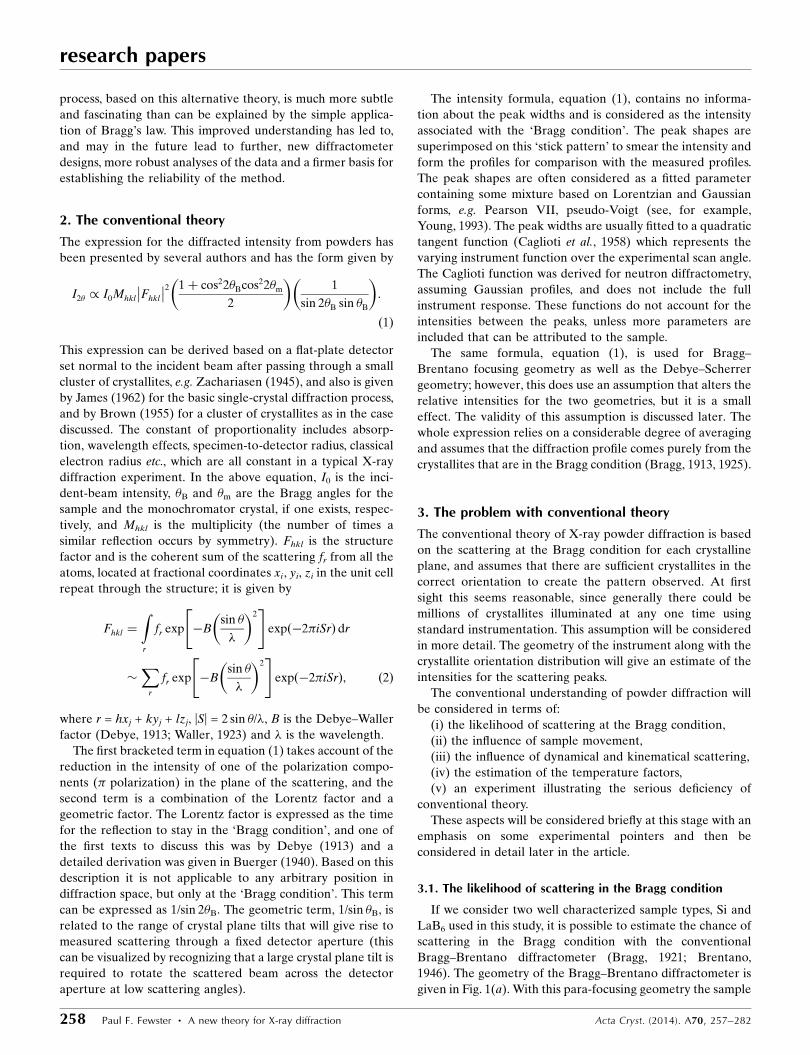
The area in reciprocal space can be determined numerically by

Heron’s method (Heath, 1921) and the results are plotted in

Fig. 9(b). The evaluated capture area in reciprocal space is

overlaid with the conventional 1/sin (2�) Lorentz factor and

clearly this derivation gives exactly the same results. What is

important here is that the derived capture volume is

completely general and is not reliant on a diffraction peak

moving in and out of the Bragg condition as in the conven-

tional definition of the Lorentz factor. Also it is independent

Acta Cryst. (2014). A70, 257–282 Paul F. Fewster � A new theory for X-ray diffraction 265

research papers

Figure 9(a) The instrument capture area for a spherical crystallite in the planenormal to the crystal plane tilt, i.e. for X = 0. The integration steps, in �and 2�, are inclined with corners of the area defined by (sxi, szi), where i =1, 2, 3, 4. (b) gives the variation in this capture area as a function of 2�(points; calculated from random values of �) and the Lorentz function1/sin 2� (line). S is the diffraction vector that defines the area in reciprocalspace for an incident-beam vector of k0 and a detected-beam directiondefined by the vector kH.

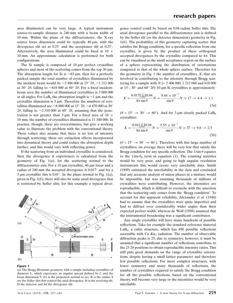
Figure 10The capture-volume variation with incident angle � and scattering angle2�. The detector slit dimension is defined by �2�s in the diffractometerplane, and the slit dimension, or Soller slit, normal to the diffractometerplane, sa. As the angle 2�–� is reduced the range in X, i.e. �X, becomeslarge. The Debye–Scherrer ring is given by the variation in � (dashedline).

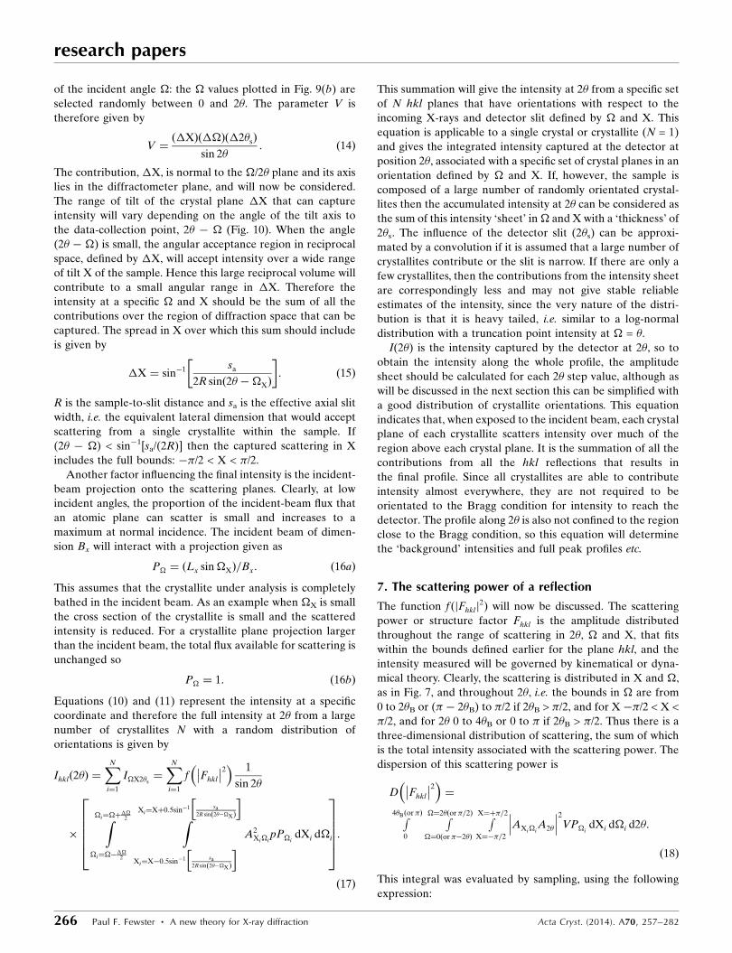
of the incident angle �: the � values plotted in Fig. 9(b) are

selected randomly between 0 and 2�. The parameter V is

therefore given by

V ¼�Xð Þ ��ð Þ �2�sð Þ

sin 2�: ð14Þ

The contribution, �X, is normal to the �/2� plane and its axis

lies in the diffractometer plane, and will now be considered.

The range of tilt of the crystal plane �X that can capture

intensity will vary depending on the angle of the tilt axis to

the data-collection point, 2� � � (Fig. 10). When the angle

(2� � �) is small, the angular acceptance region in reciprocal

space, defined by �X, will accept intensity over a wide range

of tilt X of the sample. Hence this large reciprocal volume will

contribute to a small angular range in �X. Therefore the

intensity at a specific � and X should be the sum of all the

contributions over the region of diffraction space that can be

captured. The spread in X over which this sum should include

is given by

�X ¼ sin�1 sa

2R sin 2� ��Xð Þ

�: ð15Þ

R is the sample-to-slit distance and sa is the effective axial slit

width, i.e. the equivalent lateral dimension that would accept

scattering from a single crystallite within the sample. If

(2� � �) < sin�1[sa/(2R)] then the captured scattering in X

includes the full bounds: ��/2 < X < �/2.

Another factor influencing the final intensity is the incident-

beam projection onto the scattering planes. Clearly, at low

incident angles, the proportion of the incident-beam flux that

an atomic plane can scatter is small and increases to a

maximum at normal incidence. The incident beam of dimen-

sion Bx will interact with a projection given as

P� ¼ ðLx sin �XÞ=Bx: ð16aÞ

This assumes that the crystallite under analysis is completely

bathed in the incident beam. As an example when �X is small

the cross section of the crystallite is small and the scattered

intensity is reduced. For a crystallite plane projection larger

than the incident beam, the total flux available for scattering is

unchanged so

P� ¼ 1: ð16bÞ

Equations (10) and (11) represent the intensity at a specific

coordinate and therefore the full intensity at 2� from a large

number of crystallites N with a random distribution of

orientations is given by

Ihkl 2�ð Þ ¼XN

i¼1

I�X2�s¼XN

i¼1

f Fhkl

�� ��2� � 1

sin 2�

�

Z�i¼�þ��2

�i¼����2

ZXi¼Xþ0:5sin�1 sa2R sin 2���Xð Þ

h i

Xi¼X�0:5sin�1 sa2R sin 2���Xð Þ

h i A2Xi�i

pP�idXi d�i

266664

377775:

ð17Þ

This summation will give the intensity at 2� from a specific set

of N hkl planes that have orientations with respect to the

incoming X-rays and detector slit defined by � and X. This

equation is applicable to a single crystal or crystallite (N = 1)

and gives the integrated intensity captured at the detector at

position 2�, associated with a specific set of crystal planes in an

orientation defined by � and X. If, however, the sample is

composed of a large number of randomly orientated crystal-

lites then the accumulated intensity at 2� can be considered as

the sum of this intensity ‘sheet’ in � and X with a ‘thickness’ of

2�s. The influence of the detector slit (2�s) can be approxi-

mated by a convolution if it is assumed that a large number of

crystallites contribute or the slit is narrow. If there are only a

few crystallites, then the contributions from the intensity sheet

are correspondingly less and may not give stable reliable

estimates of the intensity, since the very nature of the distri-

bution is that it is heavy tailed, i.e. similar to a log-normal

distribution with a truncation point intensity at � = �.

I(2�) is the intensity captured by the detector at 2�, so to

obtain the intensity along the whole profile, the amplitude

sheet should be calculated for each 2� step value, although as

will be discussed in the next section this can be simplified with

a good distribution of crystallite orientations. This equation

indicates that, when exposed to the incident beam, each crystal

plane of each crystallite scatters intensity over much of the

region above each crystal plane. It is the summation of all the

contributions from all the hkl reflections that results in

the final profile. Since all crystallites are able to contribute

intensity almost everywhere, they are not required to be

orientated to the Bragg condition for intensity to reach the

detector. The profile along 2� is also not confined to the region

close to the Bragg condition, so this equation will determine

the ‘background’ intensities and full peak profiles etc.

7. The scattering power of a reflection

The function f ðjFhklj2Þ will now be discussed. The scattering

power or structure factor Fhkl is the amplitude distributed

throughout the range of scattering in 2�, � and X, that fits

within the bounds defined earlier for the plane hkl, and the

intensity measured will be governed by kinematical or dyna-

mical theory. Clearly, the scattering is distributed in X and �,

as in Fig. 7, and throughout 2�, i.e. the bounds in � are from

0 to 2�B or (� � 2�B) to �/2 if 2�B > �/2, and for X ��/2 < X <

�/2, and for 2� 0 to 4�B or 0 to � if 2�B > �/2. Thus there is a

three-dimensional distribution of scattering, the sum of which

is the total intensity associated with the scattering power. The

dispersion of this scattering power is

D Fhkl

�� ��2� �¼

R4�B or�ð Þ

0

R�¼2� or�=2ð Þ

�¼0 or��2�ð Þ

RX¼þ�=2

X¼��=2

AXi�iA2�

��� ���2VP�idXi d�i d2�:

ð18Þ

This integral was evaluated by sampling, using the following

expression:

research papers

266 Paul F. Fewster � A new theory for X-ray diffraction Acta Cryst. (2014). A70, 257–282

D Fhkl

�� ��2� �¼

R4�Bðor�Þ

0

A22� d2�

!1

sin 2�

�PNi¼1

R�i¼�þ��2

�i¼����2

RXi¼Xþ0:5 sin�1ðsa2RÞ

Xi¼X�0:5 sin�1ðsa2RÞ

A2Xi�i

P�idXi d�i

" #( ):

ð19Þ

However, in an experiment, the evaluation of the integrated

intensity from a set of crystallographic planes usually only

captures the intensity close to the ‘Bragg condition’, assuming

that the background contributes no additional scattering

associated with the structure information. The integrated

intensity is then usually related to |Fhkl|2 in the kinematical

approximation. However, this assumes that the whole of Fhkl is

captured, which is not correct. The factor f is the ratio of the

integrated intensity over the measured limits, compared to the

full integral, equation (19). This is also the case for single

crystals and will be discussed later. From the last section it can

be seen that, in the powder diffraction experiment, when the

distribution of orientations is very large, the captured volume

of the scattering in � and X will include the whole distribu-

tion. However, because the instrument capture varies with

�X, equation (15), the data collection will oversample, so the

intensity is overestimated depending on � and 2�. The factor f

will therefore include two components: the limited capture

range for obtaining the integrated intensity and the over-

sampling due to the axial divergence:

f ¼Rþ�2�B

��2�B

A22� d2�

!1

sin 2�

�PNi¼1

R�i¼�þ��2

�i¼����2

RXi¼Xþ0:5 sin�1 sa2R sin 2���Xð Þ

h i

Xi¼X�0:5 sin�1 sa2R sin 2���Xð Þ

h i A2Xi�i

P�idXi d�i

8>>><>>>:

9>>>=>>>;

0BBB@

1CCCA

= D Fhkl

�� ��2� �h i: ð20Þ

The �X map, Fig. 7, represents the distribution of intensity at

a specific 2� for a specific hkl reflection. The intensity every-

where on the �X map represents the residual contribution to

the specular, and therefore also Bragg, contribution. The

overall resultant observed intensity is then the phase sum at

this specific 2�. For example, at the Bragg condition, all the

contributions scatter in phase and further from this the

differing phase contributions create an interference pattern.

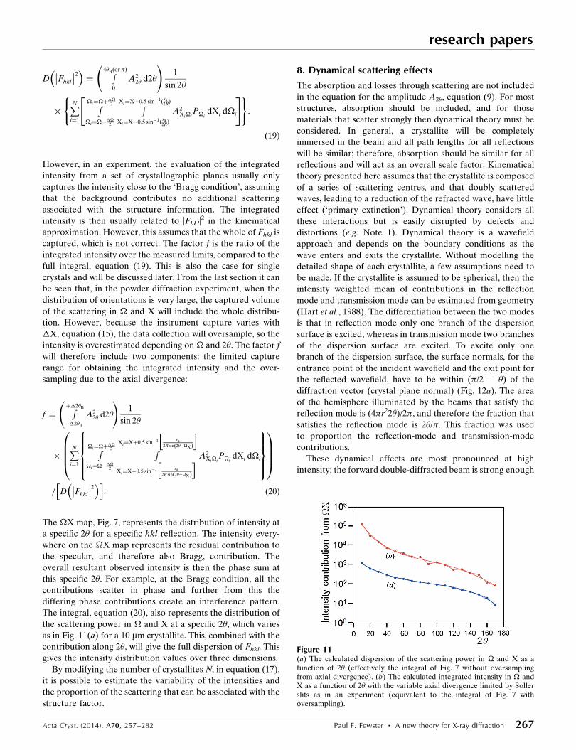
The integral, equation (20), also represents the distribution of

the scattering power in � and X at a specific 2�, which varies

as in Fig. 11(a) for a 10 mm crystallite. This, combined with the

contribution along 2�, will give the full dispersion of Fhkl. This

gives the intensity distribution values over three dimensions.

By modifying the number of crystallites N, in equation (17),

it is possible to estimate the variability of the intensities and

the proportion of the scattering that can be associated with the

structure factor.

8. Dynamical scattering effects

The absorption and losses through scattering are not included

in the equation for the amplitude A2�, equation (9). For most

structures, absorption should be included, and for those

materials that scatter strongly then dynamical theory must be

considered. In general, a crystallite will be completely

immersed in the beam and all path lengths for all reflections

will be similar; therefore, absorption should be similar for all

reflections and will act as an overall scale factor. Kinematical

theory presented here assumes that the crystallite is composed

of a series of scattering centres, and that doubly scattered

waves, leading to a reduction of the refracted wave, have little

effect (‘primary extinction’). Dynamical theory considers all

these interactions but is easily disrupted by defects and

distortions (e.g. Note 1). Dynamical theory is a wavefield

approach and depends on the boundary conditions as the

wave enters and exits the crystallite. Without modelling the

detailed shape of each crystallite, a few assumptions need to

be made. If the crystallite is assumed to be spherical, then the

intensity weighted mean of contributions in the reflection

mode and transmission mode can be estimated from geometry

(Hart et al., 1988). The differentiation between the two modes

is that in reflection mode only one branch of the dispersion

surface is excited, whereas in transmission mode two branches

of the dispersion surface are excited. To excite only one

branch of the dispersion surface, the surface normals, for the

entrance point of the incident wavefield and the exit point for

the reflected wavefield, have to be within (�/2 � �) of the

diffraction vector (crystal plane normal) (Fig. 12a). The area

of the hemisphere illuminated by the beams that satisfy the

reflection mode is (4�r22�)/2�, and therefore the fraction that

satisfies the reflection mode is 2�/�. This fraction was used

to proportion the reflection-mode and transmission-mode

contributions.

These dynamical effects are most pronounced at high

intensity; the forward double-diffracted beam is strong enough

Acta Cryst. (2014). A70, 257–282 Paul F. Fewster � A new theory for X-ray diffraction 267

research papers

Figure 11(a) The calculated dispersion of the scattering power in � and X as afunction of 2� (effectively the integral of Fig. 7 without oversamplingfrom axial divergence). (b) The calculated integrated intensity in � andX as a function of 2� with the variable axial divergence limited by Sollerslits as in an experiment (equivalent to the integral of Fig. 7 withoversampling).

to moderate the incident refracted beam, and the diffracted

beam removes a significant proportion of the incident

refracted beam. This also is only significant close to the Bragg

condition. Outside this region, it is coincident with kinematical

theory and therefore dynamical theory only needs to be

applied to scattering where � � �B.

The amplitude A2� based on dynamical theory in reflection

mode is

A2� ¼�ie tan½�gðb2 � AEÞ

1=2Lz�

ðb2 � AEÞ1=2þ ib tan½�gðb2 � AEÞ1=2Lz�

; ð21Þ

where

A ¼ F�h�k�l

sinð2� ��Þ�� ��

sin �

re�2

�VC;

E ¼ �Fhkl

re�2

�VC;

g ¼��

� sinð2� ��Þ�� �� ;

re is the electron radius, � is the X-ray wavelength and C is the

polarization factor that is 1 or cos 2�. The parameter b is given

by

b ¼ F000

re�2

�V

sinð2���Þj jsin � � 1

h i2

� 2 sin �B

�� ��� sin �j j � sinð2� ��Þ�� ��� �

sinð2� ��Þ:

These are the formulae for the two-beam plane-wave dyna-

mical theory with two tie points, e.g. Fewster (2003). This

calculation has to be performed for both polarizations and

added. If a monochromator is used then C takes on values of 1

and cos 2�mcos 2�. �B is the Bragg angle, specific to the set of

planes calculated, and �m is the Bragg angle for the mono-

chromator. If the incident wave impinges on the crystal

surface, or crystal plane below the critical angle for total

external reflection (typically � 0.2�), then the intensity scat-

tered into 2�, provided 2� > 2� critical angle, should be �

zero, although the contribution is very weak from the

projection effect, equation (16a), so neglecting this is not

serious. Any wave emerging from the exit surface, or a crystal

plane below the critical angle (i.e. for the latter 2� � � <

critical angle), may not emerge as well defined scattering,

depending on the shape of the exit surface. The latter intensity

contribution is insignificant compared to the instrumental

effects of equation (15). Therefore the intensity contributions

from within the critical angle are set to zero in the ‘sinc’

function and dynamical models, since this is the closest

approximation without modelling the crystal shape.

A more fundamental approach to the dynamical model

based on the atomic positions and scattering factors, not

requiring structure factors or Bragg angles, can yield the

amplitudes by slicing the crystallite into very thin parallel

lamellae (�0.001 nm) (Holy & Fewster, 2008). However, the

calculation time is increased substantially and the results are

essentially unchanged from those calculated here, unless the

crystallites are very small, in which case the scattering is well

represented by kinematical theory or the Debye formula

(Debye, 1915). This plane-wave dynamical theory is still an

approximation for many experiments and spherical-wave

theory would be less of an approximation; however, within all

the other assumptions regarding crystallite shape and the

possible lens nature (adding to some divergence) of the scat-

tered beam, the dynamical model used here is sufficient.

The amplitude A2� in transmission mode is based on

Zachariasen (1945) and is given by

A2�

� �2¼ E2 expð�t0Þ

sin avð Þ þ sinh awð Þ½ �2

AEþ b2j j: ð22Þ

The parameters not given above are

a ¼�Lz

� sin �

v ¼ real AEþ b2� �

w ¼ imag AEþ b2� �

0 ¼2�

�imag

re�2F000

�V

� �

t ¼ 0:51

sin �þ

1

sin 2� ��ð Þ

�Lz:

The parameter 0 is the average (kinematical) linear

absorption coefficient, which is a valid assumption for the case

studied here. For crystals greater than the absorption depth

(65 mm for Si) the separate absorption coefficients should be

considered; these are associated with the two branches of the

dispersion surface and their two polarization states, leading to

different values. By reducing the value of F�h�k�l that

corresponds to the scattering from the underside of the

reflecting planes, which interferes with the refracted wave,

then the profile becomes indistinguishable from kinematical

theory and the sinc function, for both the reflection and

research papers

268 Paul F. Fewster � A new theory for X-ray diffraction Acta Cryst. (2014). A70, 257–282

Figure 12(a) The simplified basis for establishing the proportion of reflected (R)and transmitted (T) waves for a spherical crystallite. (b) The profile basedon dynamical theory in reflection mode (red, lower central peak)compared with kinematical theory for a flat plate sample, and (c) theprofile for the transmission case.

transmission modes. The amplitudes based on dynamical

theory, for both transmission and reflection modes, have a

similar dependence, i.e. the dynamical effects reduce the low

2� and intense reflections. The dynamical effects can be seen

by calculating the profile from an 8 mm Si parallel-sided flat

plate, for each reflection, and comparing it with kinematical

theory (Fig. 12b for reflection, and Fig. 12c for transmission).

The magnitude of the dynamical effects can be reduced and

will have a dramatic effect on the calculated intensities. The

most influential variable, though, is to change the kinematical/

dynamical proportions by changing the contribution of

F�h�k�l. It can be shown that the dynamical impact, defined

by ðIkin � IdynÞ=ðIkin þ IdynÞ, is less than 6% for Si crystallite

dimensions �1 mm, giving some guidance for the influence.

This ratio gives an indication of the largest average

length scale over which defects can be separated, without

needing to invoke dynamical theory in Si, based on analysis of

just the Bragg condition. The presence of defects has an

additional effect of introducing diffuse scatter, which is

discussed later.

9. The calculation of the scattering profile

Because of the widespread use of the Bragg–Brentano

diffraction geometry, the emphasis here will be on calculations

and results from this configuration. The calculations are

lengthy and full use is made of parallel computing. In the ideal

case, the intensity distribution in X and � should be calculated

for each scattering plane hkl and at each step in 2�. In this way,

the full multiplicity can be incorporated, as in Fig. 8, and also

the trade-off between numbers of crystallites and flux can be

included, equations (23) and (24). To overcome the limitations

in computing power, a calibration curve was calculated at

various 2� values, assuming that this represented the variation

in the captured intensity with scattering angle. The captured

intensity was obtained by uniform sampling in X and �, and

superimposing the instrument capture volume ���X, and

integrating [�� is defined by the focus and crystallite size

and �X is a function of (2� � �)]. This procedure is repeated

until the intensity distributions start to converge, i.e. most

crystallite orientations have been explored and captured. This

method is applicable to randomly orientated crystallites. For

samples with texture or preferred orientation, a prior prob-

ability should be imposed (rather than uniform sampling), and

this would ideally need to be done for each set of hkl planes, so

that the multiplicity is incorporated naturally, as in Fig. 8.

Early attempts at this latter approach proved prohibitive in

time. For the calculation here, where it is assumed that no

preferred orientation exists, the multiplicity has been incor-

porated as a multiplicative factor when applying it to the

specific reflection concerned. The calculations are performed

in 64-bit Python with heavy use of vectorization with NumPy

and Parallel Python using up to 32 cores; this was far from

optimal but appropriate for testing the theory at this stage.

The results from obtaining a calibration curve are now

considered.

9.1. Intensity variations associated with the Bragg–Brentanogeometry

The above derivation assumes that the number of crystal-

lites illuminated is constant with respect to the sample as a

whole. In the para-focusing geometries, e.g. Bragg–Brentano

geometry, this is not the case, and the number of crystallites

illuminated changes with incident angle according to

NumCryst / Rsin

sin � � ð Þþ

sin �

sin � þ �ð Þ

�: ð23Þ

Here, � and are the divergence angles of the beam below

and above, respectively, the source to the goniometer axis,

which makes an angle � to the sample surface. The number of

contributing crystallites is increased at low � angles; however,

the distribution of X-ray flux is reduced according to

IBB �ð Þ ¼X

n

I0 ��ð Þ ¼sin � þ ��ð Þ

R sin � sin ��

�

�1

sin � þ n� 1ð Þ��½ �þ

1

sin � þ nþ 1ð Þ��½ �

� ��1

;

ð24Þ

where �� is a small constant angular increment in the diver-

gence. This has a similar inverse form to equation (23), and

this is why the assumption that the two completely different

geometries, Bragg–Brentano and Debye–Scherrer, can use a

similar formula in conventional theory. However, there are

small differences, e.g. the flux varies across the sample, and

this is most pronounced for smaller radii and larger samples.

For a fully illuminated 10 mm sample with a 240 mm goni-

ometer radius, the intensity variation across the surface is

1.8% and 0.45% at 28� and 88� 2�, respectively. Perhaps a

more important point here, though, is that if the NumCryst/

flux ratio is roughly constant (this varies by 10�4 from 28� to

160� 2�), then this would suggest that the diffraction profile

in the Bragg–Brentano geometry would have increasing

unreliability with increasing 2� as the distribution of crystal-

lites satisfying the Bragg condition is reduced, if the conven-

tional theory were to be correct. For the calculation in the new

theory, this larger number of illuminated crystallites (and

reduced flux per crystallite) can be included.

9.2. The intensity associated with Bragg and non-Bragg

It is important now to assess the contribution to the

captured intensity from crystallites in random orientations

compared with those contributing at the Bragg condition. This

evaluation can be achieved by uniformly sampling over � and

X, then integrating over the vicinity to emulate the angular

acceptance of the crystallite to the divergence in both direc-

tions. This will also give an estimate of the proportion of the

intensity associated with the Bragg condition, compared with

that from non-Bragg, for a stationary sample: essentially, the

intensity distribution for a specific experimental configuration.

The variation in the intensity summation for each ‘sheet’ at a

representative set of 2� values is given in Fig. 11(b). These

calculations assume that the crystallites are small compared

Acta Cryst. (2014). A70, 257–282 Paul F. Fewster � A new theory for X-ray diffraction 269

research papers

with the size of the incident beam, and also include the

probability, Pr, of capturing significant scattering over the

calculation range, i.e.

Pr 2�ð Þ ¼2�

2�; 2� �

�

2; Pr 2�ð Þ ¼

�� 2�

2�; 2� >

�

2: ð25Þ

Initially, uniform sampling was carried out whilst monitoring

the convergence and variance of the mean intensity; however,

because the Bragg condition is such a rare event (i.e. the

central specular condition � = � and X = 0 in Figs. 4b and 7) a

vast number of crystallites are required to explore it and to

reduce the variability. After many millions of samples, with an

integration of the instrument capture at each position, the

solution is far from converged, and since this cannot easily be

achieved analytically, an integration method based on the idea

of importance sampling was used. The map was separated into

areas and sampled to achieve a mean; the mean was scaled to

the dimensions of the area. This allowed convergence at a far

faster rate in a practicable timescale.

The variation in the intensity captured as a function of 2� is

given in (i) of Fig. 13(a). This is a calibration curve that can be

applied to each intensity value at 2�. If the specular peak

corresponds to the appropriate 2�B coherent Bragg condition,

then the mean intensity value may not follow the kinematical

theory and so it is useful to separate the ‘Bragg’ and ‘non-

Bragg’ contributions, (ii) and (iii) in Fig. 13(a). The Bragg

condition is assumed to be satisfied whenever the Bragg peak

appears in the accepted divergence of the instrument. Hence

provided the incident beam and the scattered beam exist

above the scattering plane and they are on the opposite sides

of the plane normal, then the ‘non-

Bragg’ condition is satisfied, whereas

the ‘Bragg’ condition only exists under

exacting requirements. This is re-

expressed in Fig. 13(b), by plotting

mean values of the specular and non-

specular, multiplied by their numbers to

give the effective intensity contributions

from each. The intensity measured in

the specular (and therefore the Bragg

condition) is composed of �30% ‘non-

Bragg’ and �70% ‘Bragg’, with a stan-

dard deviation of 10% for these values

for 10 mm crystallites (Fig. 13c). The

calculation is based on sampling the

equivalent of 153 000 000 events at 2� =

10�, to a maximum of 1 374 000 000 at

90�. With more sampling this standard

deviation will reduce; however, this

does give an estimate of the proportions

of the scattering attributed to ‘Bragg’

and ‘non-Bragg’, in the limit of a very

large number of crystallites (Fig. 13c). A

typical experiment may capture none,

or very few Bragg events; however, the

mean intensity will only be displaced by

a small amount [Fig. 13a (i) compared

with (iii)]. This indicates that the impact of capturing Bragg

events will not have a large effect on the measured intensity.

Also, if the number of Bragg events changes roughly in

proportion across the 2� range, then the relative intensities

will be unchanged. These calculations were repeated for 3 mm

crystallites (Figs. 13d and 13e), and for 10 mm crystallites that

contained defects (i.e. diffuse scattering was introduced) (Fig.

13f). The introduction of diffuse scattering caused no obser-

vable difference in the ratio. For 3 mm crystallites, the ratio is

changed to 65 (15)% for the ‘specular’ contribution,

suggesting that the ‘specular’ and therefore ‘Bragg’ contri-

butions are less significant for small crystallites.

The importance sampling method used does reduce the

variability of the specular, and increase the variability of the

non-specular, compared with a totally random sampling

method. This is because the density of samples is much higher

in the former and would require a comparable number of

crystallites to give rise to the number of events quoted, and

much lower in the latter. This explains why the profiles are

not perfectly smooth [Figs. 13a (iii) and 13d (iii)]. It was

impractical to sample this equivalent number of events. In

fact, the equivalent number of events quoted is derived from

the sampling density within 0.5� of the specular position,

whereas elsewhere the sampling is sparser and scaled. The

total number of samples for each of the 17 2� values was

81 000.

The overall ‘converged’ mean intensity [Fig. 13a (iv)] [and

Fig. 13d (iv)] was obtained by fitting a fourth-order polynomial

to 13a (i) [and 13d (i)], once sufficient numbers of calculations

had been completed and the profiles had stabilized. This,

research papers

270 Paul F. Fewster � A new theory for X-ray diffraction Acta Cryst. (2014). A70, 257–282

Figure 13(a) The mean calculated intensity as a function of 2�: (i) overall mean from all contributions, (ii)only those contributions that capture the ‘specular’ peak, (iii) the mean intensity of those from the‘non-specular’ and (iv) the best fit profile through the overall mean intensity. (b) are the meanintensities � numbers for the ‘specular’ (i) and the ‘non-specular’ (ii). (c) gives the ratio of theproportions of ‘specular’ (i) and ‘non-specular’ (ii) to the overall intensity. (d) and (e) are similar to(a) and (c), except the calculations are based on 3 mm crystallites. ( f ) compares directly with (c),except the calculation is for 10 mm crystallites with defects, i.e. diffuse scattering is included.

as mentioned earlier, represents the situation with a large

number of randomly orientated crystallites.

The overall intensity captured during an experiment at the

‘Bragg position’ (or ‘specular position’) is the product of the

number of contributions and mean intensity associated with

the ‘Bragg condition’ (or ‘specular condition’), plus the

product of the number of contributions and mean intensity

associated with the ‘non-Bragg condition’ (or ‘non-specular

condition’):

Ioverall ¼ BraggNBragg þ non-BraggNnon-Bragg: ð26Þ

These mean ‘Bragg’, ‘non-Bragg’ and ‘overall’ intensity

contributions are given in Fig. 13(a), where a significant

difference can be seen in the ‘Bragg’ and ‘non-Bragg’ means.

However, the product of the number of contributors of ‘Bragg’

and ‘non-Bragg’ with their respective mean intensities result

in very similar values (Fig. 13b). The result of this is that the

overall mean intensity is very similar to the mean intensities of

the ‘non-Bragg’ contributions, Figs. 13(a) (i) and 13(a) (iii),

and 13(d) (i) and 13(d) (iii).

The calculated mean intensities converged to the values

given in Fig. 13(a) (i), which could then be fitted with a fourth-

order polynomial as a function of 2�, Fig. 13(a) (iv) for 10 mm

crystallites, 13(d) (iv) for 3 mm crystallites and Fig. 11(b) for

10 mm crystallites with defects. The profiles all follow the same

shape. If we assume that this fit represents the converged

mean intensities, then the overall variability expected from the

experimental intensities would be related to the number of

contributions of ‘Bragg’ (‘specular’) and ‘non-Bragg’ (‘non-

specular’) and each will follow a Poisson distribution, i.e. � =

N1/2. The overall variance for the two contributions is there-

fore given by

�2overall ¼

@Ioverall

@NBragg

!2

�2NBraggþ

@Ioverall

@Nnon-Bragg

!2

�2Nnon-Bragg

: ð27Þ

Combining equations (26) and (27) will give

�2overall ¼

2Bragg�

2NBraggþ 2

non-Bragg�2Nnon-Bragg

: ð28Þ

The expected reliability of the intensity measurements in an

experiment can be expressed as �overall/Ioverall, by using equa-

tions (26) and (28), and is given by

�overall

Ioverall

¼ð2

Bragg�2NBragg þ

2non-Bragg�

2Nnon-BraggÞ

1=2

BraggNBragg þ non-BraggNnon-Bragg

: ð29Þ

The conventional theory is based on only the first term in both

the numerator and denominator, and this will be referred to as

the ‘Bragg’ �/I.

9.3. The ratio of Bragg to non-Bragg events

The above calculation gives estimates for the mean inten-

sities associated with the ‘Bragg condition’ (or ‘specular

condition’) and the ‘non-Bragg condition’ (or ‘non-specular

condition’), for any experimental configuration. To estimate

the level of reliability, as �/I, the number of ‘Bragg’ and ‘non-

Bragg’ events is required, equation (29). Since any experiment

may have different numbers of crystallites, it is more helpful to

calculate the ratio of the number of events, which is more

universal. The ratio of ‘specular’ to ‘non-specular’ events

associated with a particular experimental configuration can be

estimated as in the following two sections: these determine the

ratio directly, whereas the above calculations include intensity

estimations as well, which is considerably slower to calculate.

Because these calculations require a large number of repeats,

the results presented here are given as a range of both

calculations, to give an indication of typical values for the

instrument configurations described later.

For the same number of calculated events across all 2�values the number of Bragg events at 10� is approximately

twice that for 2� > 30�, whereas the intermediate value at 20� is

�70% more than for 2� > 30�. The ‘specular’ to ‘non-specular’

ratio from numerous calculations for the 2� > 30� region varies

from 1.3 � 10�7 to 1.7 � 10�7, which is in broad agreement

with equations (3a) and (3b). The increased ‘specular’

contributions captured at low 2� values is a consequence of

the larger capture volume in the axial divergence. The larger

capture volume at low 2� values also increases the number of

‘non-specular’ contributions in a similar way. The consequence

of this is that the ‘Bragg’ and ‘non-Bragg’ contributions, given

in equation (26), are fairly similar across the 2� range, as

shown in Figs. 13(c), 13(e) and 13( f), for 10 mm perfect crys-

tallites, 3 mm perfect crystallites and 10 mm crystallites with

defects, respectively.

It is reasonable to suppose that, for different size crystal-

lites, focus size and Soller slits (the main determining factors)

will not change the ratios significantly. It should be remem-

bered that data collected around a complete Debye–Scherrer

ring will be composed of intensity with a combination of

these ‘specular’ and ‘non-specular’ contributions, and each

measurement capture region will follow a very similar ratio.

Two configurations commonly used with the Bragg–

Brentano geometry will now be considered in more detail, so

that a more realistic estimate of the reliability in the measured

intensity values can be assessed.

9.4. The case of a stationary sample

For a sample illuminated with a 10 � 10 mm footprint

composed of 10 mm crystallites three deep (half the absorption

depth for Si), with a 50% volume density, the scatter will be

created from 1 500 000 crystallites when the sample is

stationary and held at a specific 2�. For a reflection at 69� 2�and a multiplicity of 8 (004 reflection), the average number of

Bragg contributions will be 0.5 � 1 500 000 � 8 � (�1.3 �

10�7); the latter is the ratio given above, which can be

considered as the likelihood of capturing the ‘Bragg condition’

from a crystallite. This results in �0.75 Bragg events and 1.2�

107 non-Bragg events, for a stationary non-rotating sample

(the 0.5� accounts for the scattering going towards �2�). The

�/I values for the Bragg and non-Bragg are �88% and

�0.02% respectively, from equations (26) and (28). The

overall �/I is �64%. This combination of stable underlying

intensity reduces the impact of the very variable ‘Bragg’ or

Acta Cryst. (2014). A70, 257–282 Paul F. Fewster � A new theory for X-ray diffraction 271

research papers

‘specular’ contributions to give a much more reasonable

overall variability.

This overall �/I of �64% is the value calculated based on

pure monochromatic radiation and a very narrow detector slit.

During an actual experiment there is a dispersion of wave-

lengths and a range of scattering angles entering the detector

slit, i.e. the limited resolution of the diffractometer helps to

reduce the variability. If the radius of the diffractometer is

240 mm, with an X-ray focus of 40 mm, a detector slit of 55 mm

for 10 mm crystallites, then from geometry, the spread in 2�trajectories accepted is 0.041�. The calculated intrinsic scat-

tering width for the 004 reflection from Si is �0.0025�;

therefore in simplistic terms it can be considered that the

effective number of Bragg events could be magnified by 0.041/

0.0025 � 16. If the integrated intensity is measured (or the

whole shape of the profile is used in the analysis), then the

angular acceptance at the detector slit from a 10 mm crystallite

at this radius is 0.024�, which is the unique sampling range. For

a typical experimental profile width of �0.1� this will result in

0.1/0.024 � 4 unique captures over the peak. The accepted

wavelength spread (�� �1.6 � 10�3 A for Cu K�1 radiation)

within these allowable trajectories for each sample point is

greater by a factor of 2 than the natural wavelength dispersion

of 7 � 10�4 A (FWHM for Cu K�1), so the effect is small in

comparison, adding�20% to the width. The inclusion of these

experimental aberrations will increase the number of Bragg

events to �51, and the non-Bragg to 1.6 � 109, which in turn

reduces the �/I to �14% for the Bragg contributions.

However, when the non-Bragg contributions are included, the

overall �/ �8.0%. This estimate assumes that the probability

of capturing a Bragg event through scanning is uncorrelated,

which may not be the case, and also does not include shot

noise etc.

9.5. The case of a rotating sample

Sample rotation could change the variability and perhaps

make the ‘Bragg’ condition more likely. In a typical experi-

ment using the Bragg–Brentano geometry, the sample is

rotated about an axis ’, normal to its surface. For a crystallite

at a distance r from the centre of rotation, the incident beam

it experiences will vary during rotation. This depends on

the angle of its scattering plane normal to the axis of rotation,

W, and the projection of the scattering plane normal onto the

normal of the rotation axis, and perpendicular to the

diffractometer � axis, U (Fig. 14a), such that a crystallite

position within the sample can be defined by

0< r<Rsample

��<U<�0<W<�=2;

ð30Þ

where Rsample is the radius of the sample. By geometry, the

incident angle onto an individual crystallite, i, at a distance, r,

from the centre of rotation at an angle, ’, away from the plane

including the rotation axis and the diffraction plane is

�ri’ ¼ � � tan�1 r cos ’ sin �

Rþ r cos ’ cos �

� �þ tan�1 tan Wi cos ’þ Uið Þ

� �; ð31Þ

where R is the diffractometer radius. The tilt, X, as defined

before (Fig. 6a) can be envisaged as in Fig. 14(a) and is given

by

Xi ¼ tan�1cos Ui þ ’�

�2

� �cos Ui

�: ð32Þ

These equations give � and X, as in equations (6), (8) and

hence (9) as ’ is rotated for a specific crystallite plane defined

by a position r, and angular descriptions given by U and W. A

further constraint on the crystallites that contribute is the

illuminated length in the diffraction plane, defined by the

divergence slits, and the mask that limits the illuminated

length normal to the diffraction plane. The calculation is

performed by taking a random distribution of crystallite

orientations in rings with a dimension of the crystallite

diameter, and making very fine steps in ’ that modify � and X

for 0 < ’ < 2�. Clearly, simulating the full pattern from many

crystallites during rotation is a very lengthy calculation, so an

estimate was obtained by noting when a crystallite is orien-

tated into the specular (and also therefore the Bragg) condi-

tion, defined as within the angular acceptance �� (= 0.017�

research papers

272 Paul F. Fewster � A new theory for X-ray diffraction Acta Cryst. (2014). A70, 257–282

Figure 14(a) The parameters defining the geometry of a crystallite at a distance rfrom the rotation axis ’, with orientation coordinates defined by U and W.(b) The total number of ‘specular’ events (i) captured by the detector at2� = 60� from various radii as the sample is rotated, and (ii) the number of‘non-specular’ events that can reach the detector. The sample is assumedto be larger than the illuminated area, which is 10 � 10 mm; the kink inthe profile occurs because the illuminated area is square and the fullyilluminated area during a full rotation is a circle.

for 10 mm crystallites) and �X, equation (15), and if not when

0 (or � � 2�) < �X < 2�B (or �/2) for the non-specular (and

also therefore the non-Bragg condition). Since the mean

specular and non-specular intensity values have already been

established for a very large number of crystallites, the number

� mean will give the total intensity of the two contributions.

The number of specular and non-specular contributions is

given in Fig. 14(b) as a function of the radius, for an illumi-

nated length of 10 mm and a mask of 10 mm. This calculation

was repeated ten times to give an idea of the variation, which

would also give an indication of the reliability in measuring

several samples with randomly orientated crystallites. In one

revolution, assuming that only the top three crystallites

contribute, which is half the absorption depth in Si, the

accumulated number of specular and therefore Bragg events

at 2� = 60� amounts to 378 (108), whereas the number of

‘non-specular’ events amounts to 2 288 677 997 (434 565). A

contributing specular event is counted each time a step in ’registers one, and therefore a single scattering plane can

contribute to more than one specular event. In the example of

the contributors in Fig. 14(b) they range from two contribu-

tions per specular event up to 32; this indicates that they exist

over an angular range in ’ from �0.2� up to �3.2�. The ratio

of the number of ‘specular’ to ‘non-specular’ events is 1.65 �

10�7, i.e. within the spread of values mentioned previously.

This has been repeated at 30�, and again the ratio is of a

similar order, although the average angular range of the

contributions per specular event appears smaller. This ratio of

‘specular’ to ‘non-specular’ events is also the same for smaller

illumination sizes. Clearly from this analysis the incremental

rotation in ’ can introduce more crystallites into the specular

condition, and also allows some to exist over large angular

ranges; this also increases the number of non-specular

contributions and the ratio is unchanged. The ratio of the

intensity contributions is therefore unchanged from the

stationary condition, although the number of contributions

from these �1 200 000 crystallites is increased over that of the

stationary experiment, thus reducing the variability.

Undertaking a similar analysis to that above for a 10 �

10 mm footprint and rotating, the �/I for the Bragg contri-

butions is 5.1% and the overall value is 3.2%. Hence a very

large sample of randomly orientated crystallites will have

reliable results; anything greater than this would suggest

preferred orientation, provided shot noise and other effects

are accounted for. These values are changed to 0.65% for

‘Bragg’ and 0.40% overall when the aberrations from wave-

length dispersion and slits, but not multiplicity, are included. A

minor phase at the 10% level in this sample would give an

overall �/I closer to 1.2% (or 10.1% without these aberra-

tions) and for a phase proportion of 1%, would give �/I close

to 4% (or 32% without aberrations). The equivalent �/I values

if they are based purely on ‘Bragg’ contributions would be

2.0% and 6.4% (or 16.3% and 51% without aberrations),

respectively. The presence of the ‘non-Bragg’ contributions

gives a significant improvement in the reliability of the

measured intensities, and similarly for the presence of aber-

rations. As mentioned above, these aberrations may be

correlated and therefore not independent: this will reduce

their impact on the �/I values.

It should be remembered at this stage that these calcula-

tions of the intensity at the Bragg condition are all based on

a kinematical model. The suppression of the peak ‘Bragg’

intensity with respect to the tails from dynamical effects will

increase the ‘non-Bragg’ contribution and lower the varia-

bility. The above example is for the 004 reflection from Si,

which has a multiplicity of 8, and produces a greater number

of 004 ‘Bragg’ events per crystallite, compared with a structure

of lower symmetry.

9.6. Structural aspects that may modify the probability of‘Bragg’

During the course of this study, diffuse scattering, crystallite

size dispersion and mosaicity were considered as factors that

might influence the intensity reliability, the number of Bragg

events and the intensity ratios. The diffuse scattering will

redistribute the ‘Bragg’ into the ‘non-Bragg’ contribution,

whereas size dispersion and mosaicity will introduce more

‘Bragg’ events but reduce their impact. These aspects start to

become sample dependent, which could be problematic for an

overall general explanation without experimental evidence;

however, they are considered and discussed here.

Crystallite size dispersion. The effect of crystallite size

distribution was tested by calculation of the intensities with

different size crystallites and then combining; however, the

broad conclusions are the same. As the size is reduced, the

intensity dispersed into ‘non-Bragg’ increases and the height

of the Bragg peak reduces. In an equivalent calculation as

above but for 3 mm crystallites, the ‘non-Bragg’ increases at

the expense of the ‘Bragg’ contribution. The proportion of

intensity that can be attributed to ‘Bragg’ reduces to 65%

compared with 70% for the 10 mm crystallites. These calcula-

tions were based on the equivalent of 300 000 000 events at

10� and 2 703 000 000 events at 90� 2�. The proportion of the

crystallites in the Bragg condition is independent of the

crystallite size or number; it is the reduction of the intensity in

the Bragg condition and the increased intensity in the tails that

change the proportions. This is because in general the

instrument capture is significantly larger than the intrinsic

scattering width of the crystallites; the likelihood of this being

the case is considered next.

Mosaicity. The presence of mosaicity is much more difficult

to visualize, since this would require all crystal plane orien-

tations to be dispersed in a similar manner. Yet mosaicity

requires the crystallite to be composed of smaller crystallites

with similar orientations. These can be joined by low-angle

grain boundaries, which are often crystal plane orientation

dependent, or if the angles are large, then they scatter inde-

pendently. This will either lead to some preferred orientation

or be equivalent to more small crystallites. By isolating a single

crystallite from the Si powder sample under study, the ‘rocking

angle’ (scanning in �) showed no evidence of mosaic features

in the studied sample (Fig. 15), just a sharp narrow peak

�0.002� in 2� (from an accumulation of these diffraction

Acta Cryst. (2014). A70, 257–282 Paul F. Fewster � A new theory for X-ray diffraction 273

research papers

maps) and �0.02� in �; this is too small to have an effect on

the capture of the Bragg condition.

Diffuse scattering. Two forms of diffuse scattering are

considered to try to understand their influence. These are:

thermal diffuse scattering (TDS), see the Appendix, and more

realistically, scattering due to defects, such as dislocations,

point defects, clusters and surface damage. The overall

intensity with all these additions is unchanged in the kine-

matical scattering model, but is redistributed in � and X, and

in 2� if they introduce a strain. Many authors have studied the

defects in Si, including the resulting diffuse scattering, e.g. Lal

et al. (2000). Lal et al. have found that as-grown Si can have

oxygen clusters of �0.24 mm, which result in diffuse scattering

with a characteristic change in intensity fall-off in reciprocal-

space distance, s, from the reciprocal-lattice point, where this

changes from �s�2 to �s�4 (Huang, 1947; Stokes & Wilson,

1944). Annealing in oxygen above 873 K reduces the width of

the diffraction profile. The concentration of defects in as-

grown Si gives observable diffuse scattering at the 10�1I0 level,

above that expected from TDS. In reality, surface damage

could increase diffuse scattering significantly (Fewster &

Andrew, 1993b). If diffuse scattering is observed at the level

modelled here in semiconductor-grade Si, then it is likely to be

present in virtually all samples.

Typical preparation methods will almost certainly produce

significant levels of surface damage and hence diffuse scat-

tering. Knowing whether this is a true representation of the

diffuse scattering is not essential, but knowing whether it can

influence the intensity ratios is important. The analysis similar

to that above gave results very similar to those in Figs. 13(a)

and 13(b), indicating that at the 3 � 10�1I0 level of diffuse

scattering, the expected intensities are indeed unchanged in

the kinematical model, i.e. the significant part of the diffuse

scattering is generally within the same capture volume as the

Bragg peaks. The proportion of ‘specular’ to ‘non-specular’

was closer to 75%, with a standard deviation of 6%, although

as the diffuse scattering increases this will reduce this value

(Fig. 13f). The defects giving rise to the diffuse scattering can,

though, change the dynamical/kinematical ratio.

If it is considered that the minimum diffuse scattering

estimated by Lal et al. (2000) is �10% of the 111 Bragg peak

intensity, then this gives a starting value for the level of diffuse

scattering to include. The ratio of the intensities for 10 mm

spherical crystallites based on the dynamical and kinematical

theories is �0.08 (using the geometrical mean of mixed

contributions as described above: in pure reflection and

transmission this would be 0.12 and 0.04, respectively). These

evaluations are calculated by including the full capture volume

(Fig. 16a), with the addition of the influence of the detector

acceptance, �2�s. If diffuse scattering is included at 10% of

the kinematical peak level, then the ratio tends towards �0.63

(0.78 and 0.49 in reflection and transmission, respectively).

It is clear that the impact of diffuse scattering could be

significant in reducing the influence of dynamical scattering on

the intensities and may explain the near-perfect fit to the

kinematical theory. The data presented in Fig. 16 serve as a

useful guide as to how much diffuse scattering should be

included, based on the 220 reflection. The simulation of the

profile in Fig. 16(b) is obtained by first calculating the �profile, assuming kinematical scattering for a perfect crystal-

lite, and including diffuse scattering with a magnitude defined

by a ratio of its maximum to the original peak intensity; the

total intensity is assumed to be the same. The remainder of the

kinematical proportion that is not associated with the diffuse

scattering is then subjected to dynamical scattering to give an

approximation of the scattering from the perfect and imper-

fect regions.

The profile to be compared with the experimental result

includes the instrumental aberrations (Fig. 16b): the crystal

analyser has an acceptance �0.003� and is set to the Bragg

peak, and the angular acceptance by the crystallite is given by

the crystallite–focus combination, which gives the blurring of

the profile in �, and is of the order of 0.008�. The experiment

used a double pinhole in combination with a line focus and a

three-bounce 220 Ge analyser crystal to remove wavelength

dispersion (Fewster, 2004). The level of diffuse scattering was

varied until the profiles became roughly coincident (Fig. 16b).

The experimental profile, shown as dots in Fig. 16(b), has a

slower fall-off in intensity than that predicted using a defect

size of 0.24 mm (b and c in Fig. 16b). The best fit occurred with

a defect size of �0.18 mm (d in Fig. 16b) with a diffuse peak to

research papers

274 Paul F. Fewster � A new theory for X-ray diffraction Acta Cryst. (2014). A70, 257–282

Figure 15(a) The intensity measured in the vicinity of the 220 Bragg peak from acrystallite by isolating it from a larger diffraction space map, measured byPatricia Kidd. The geometry used was the Beam-Selection-Diffract-ometer (Fewster, 2004), with a 100 mm double pinhole, Cu K� and 220 Geanalyser crystal. The near-perfect match of the reflection choices removesthe wavelength dispersion to reveal the intrinsic width of the Bragg peak,which is 0.002�. Along � is blurred by diffuse scattering and the pinholegeometry. This can be compared with Fig. 7, although this extremely highresolution diffraction space map is truncated because of the limitedacceptable axial divergence. The maximum intensity is �2 counts s�1. (b)is the projected sum of the central region of the map.

kinematical peak fraction of �0.5. However, it is not the

purpose of this article to analyse the diffuse scattering in

detail, but to indicate the level of dynamical scattering that is

likely to be present, by introducing diffuse scattering to

account for the measured profile. The diffuse scattering is

assumed to be kinematical.

This estimate of the diffuse scattering contribution is then

applied to all reflections, with the capture volume for the

Bragg–Brentano geometry used in this study. This gives the

ratio of the dynamical/kinematical theories, from which

the scale factors can be determined to correct the intensity

contributions for dynamical effects when the Bragg peaks

are captured (Fig. 16c). From Fig. 16(c) it appears that the

level of diffuse scattering is in excess of that required to

modify the kinematical assumption by more than a few per

cent. It is also important to note that the profile of the diffuse

scattering does not change significantly as the fraction is

increased above 0.5, so this is really a lower limit to account

for the experimental results, and therefore the dynamical

effects are likely to be less than this. This methodology also

assumes that there is a clearly defined perfect and imperfect

region, which is unrealistic but does represent the maximum

impact that dynamical effects can have. It seems reasonable to

assume that as the defects become more distributed then the

perfect region size shrinks and the dynamical effects are

further diminished.

It is worth noting that dynamical effects will have a bigger

impact on conventional theory than on this new theory for

powder diffraction. The intensity is assumed to only come

from Bragg scattering in the former, whereas this new theory

reduces the proportion of intensity from Bragg scattering to

�0.75 for 10 mm Si crystallites. As discussed earlier, this is the

limiting case, and for many experiments, when there are far

fewer crystallites, the variability of intensity associated with

Bragg events will mask the dynamical effects. For the sample

composed of 2.3 � 109 possible orientations given in Fig. 14,

the number of Bragg events is 380 with a variability of �10%

which is comparable to the influence of dynamical effects, and

therefore the impact of dynamical theory will be masked.

Also, if the diffuse scattering is significant then it will redis-

tribute the scattering outside the Bragg peak capture volume,

raising the ‘non-Bragg’ contribution, which in turn reduces

the ‘Bragg’ peak intensity and therefore the proportion of

Bragg scattering. If the impact, of encountering a Bragg peak,

on the measured intensity becomes less significant, then the

data may be less variable, which is the case when smaller

crystals are used. For smaller crystals it would be reasonable

to assume that the ‘defect to perfect’ crystal ratio increases

with the ‘surface roughness to volume’ ratio. It appears that

kinematical scattering is a good approximation to the scat-

tering observed from crystals with defects, i.e. ‘real’ crystals;

however, we can draw some other conclusions that are

covered in the following section.

10. Comparisons between theory and experiments

Equation (17) represents the intensity arriving at the detection

point 2�, and each scattering plane will have contributions to

each 2� value that fit within the bounds. The full profile can

therefore be calculated at each value of 2� from 0� to 180� (or

4�B if smaller). The emphasis in this section is on Si, since the

atom positions are defined by symmetry and the temperature

factors have been measured and calculated to high precision

(see the Appendix). The comparison in intensity will be with

the Bragg–Brentano geometry, because this is the most widely

used configuration. An explanation for the intensity features

observed in a Debye–Scherrer ring will also be illustrated.

10.1. Bragg–Brentano geometry

The basic Bragg–Brentano configuration used in this study

consisted of a goniometer of radius 320 mm, an incident beam

slit of 0.125�, a projected focus size of 0.0418 mm that results

in an illuminated area of �0.7/sin � mm (giving a maximum

and minimum area of 2.8 to 0.7 � 12 mm over the range of

reflections possible for Cu K� radiation) and this ensures that

the illuminated area is still smaller than the sample at 10� 2�.

This configuration should ensure that exactly the same total

intensity is experienced at each angular range, although the

number of crystallites will vary. The detector used was a solid-

state PANalytical PIXcel, with data collected in 0.055 mm

Acta Cryst. (2014). A70, 257–282 Paul F. Fewster � A new theory for X-ray diffraction 275

research papers

Figure 16(a) The simulated scattering within the instrument capture volume for10 mm crystallites at the exact Bragg condition within the Bragg–Brentano geometry (Si 220 reflection) with no instrumental aberrationsor diffuse scattering. (b) The simulated profile (including instrumentalaberrations from the geometry given in the caption to Fig. 15) withincreasing levels of diffuse scattering, a, b, c, d, that correspond to theratios of the peak in the diffuse scatter to the kinematical maximum of 0,0.1, 0.5 and 0.75, respectively. The barely observable double line for eachcorresponds to transmission (lower line) and reflection (upper line)dynamical contributions. (c) The residual dynamical contributions for theBragg–Brentano geometry described in the text; the intensities are givenfor the geometric average of the reflection and transmission geometries,with the dashed line for conventional theory (ac, bc, cc, dc) and the solidline for the new theory (a, b, c, d), where the fractions correspond to thosein (b).

strips, producing good para-focusing conditions. Soller slits of

0.04 radian were placed in the incident and scattered beam to

limit the cross-fire. The sample was a disc composed of an

amorphous resin and Si crystallites in equal proportions. The

Si crystallites have dimensions ranging from 5 to 15 mm, with >

80% being 10 mm.

For a 30 mm penetration these dimensions equate to

�26 000 crystallites at 28.4� 2� and 6300 crystallites at 158.6�,

illuminated at any one time at each data-collection point. This

would equate to �0.25 � Mhkl/2 (�1 for hkl = 111; Mhkl/2

takes account of the distribution of scattering towards 2� and

�2�) and �0.05 � Mhkl (�0.25 for hkl = 444) Bragg events at

each of these two angles, when all the factors of wavelength

dispersion and divergence are included as discussed

previously. The non-Bragg events are similarly increased to 6

� 106. The estimated �/I, for six independent measurements

(experimental details are contained in the following para-

graph), varies from �10% to �30% (Fig. 2), and is compar-

able to the calculated �/I for the condition with no aberrations

of �22% and greater than the condition with aberrations of

�2.7%. The latter value is the estimated best result that could

be achieved, remembering that this does not include shot

noise, and assumes that the contribution from scanning is

uncorrelated: if it is correlated this latter value may increase

up to a limit of �11%. If the number of independent

measurements was increased tenfold then the �/I value would

be within the bounds of 3% to 10%, so these calculated and

measured �/I values are in broad agreement. These are only

estimates, so to support this, a series of stationary measure-

ments of the 111 reflection were taken at various ’ angles (Fig.

17). The divergence slit was set to 0.0625�, 0.04 radian Soller

slits and the data were captured on the PIXcel as a one-

dimensional strip detector, which is why the resolution is

poorer than in the scanning method. The profile can be seen to

consist of two parts, a spiky part superimposed on a well

defined hump: this can be interpreted as the Bragg spikes

superimposed on top of non-Bragg contributions. The number

of significant peaks per scan is �1, which fits with estimates

above for the 111 reflection. It is difficult to judge exactly

where the Bragg to non-Bragg boundary should be, but from

visual inspection it appears that the non-Bragg intensity is

greater than the Bragg intensity in this experiment (Fig. 17),

whereas in the limit of very large numbers of crystallites that

are perfect, the Bragg intensity is greater than the non-Bragg

intensity (Fig. 13c). It is clear though that the intensity arriving

on each strip has a stable non-Bragg intensity contribution

with a much more variable Bragg intensity contribution

superimposed.

To determine the intensity ratios between all reflections, a

series of 2�/! scans in the centre of six different samples from

10� to 162� were collected whilst spinning the sample in ’.

These gave an average value and a variance for the integrated

intensity. The count time was 8.67 s per 0.0025� step captured

in continuous collection mode (Fig. 18a). The integrated

intensity of a reflection in a typical diffraction experiment is

given by the summation over 2� close to the peak. The region

of integration will be limited by the dynamic range of the

experiment and the general shape of the 2� profile, but as

discussed earlier this will only represent a proportion of the

scattering power. Three representative measured peaks are

given as insets to Fig. 18(a), and from these it is possible to

estimate the proportion of the scattering power captured. The

integrated intensity has been taken as the sum of the contri-

butions above the ‘background’. The location for choosing the

background level for the experiment indicates the angular

research papers

276 Paul F. Fewster � A new theory for X-ray diffraction Acta Cryst. (2014). A70, 257–282

Figure 17A series of stationary profiles, using the Bragg–Brentano geometry, of theSi sample described in the text. The experiments were measured at 0.5�

intervals over 10� in ’. The profiles appear to exist in two distinct forms, ageneral ‘background’ (smooth hump) and a spiky region superimposed,thought to be associated with ‘non-Bragg’ and ‘Bragg’ contributions,respectively. The spikes appear and disappear within similar angularranges in ’ as predicted from the calculations leading to Fig. 14(b).

Figure 18The full profile for Si powder with Cu K� radiation with (a) and without(b) the instrumental artifacts; (a) and (b) are plotted on square-root andlogarithmic scales, respectively. The calculated profile is given by the thickred smooth line, and the six experimental profiles in (a) are overlaid togive some indication of the variations between samples, which is coveredin more detail in Fig. 19. The artifacts included are all defined by theinstrument dimensions, except the background due to residual scattering(presumably hard radiation from the slits etc.), which is fitted with apolynomial. The spectral dispersion, e.g. Cu K after absorption by the Nifilter, appears at the right level within the background noise. A fewreflections are plotted on a linear scale to illustrate the agreement.

range for estimating the equivalent integrated ‘peak’ intensity

in the calculated profile. The proportion of the scattering

power that is captured in the experiment for the various 2�values is given in Fig. 11: it is also important to remember that

it is also dispersed in 2�. By measuring the intensity in a

systematic way, it should be possible to obtain a good estimate

of the proportion of the dispersed scattering power.

This theory creates the full profile as discussed before;

however, to bring it into line with the actual experiment, there

are some additional factors to consider, some of which have

been alluded to in estimating the �/.

(a) Wavelength dispersion: in effect, each wavelength

constitutes a different experiment, so a convolution is a

reasonable approximation, since the whole simulation can be

repeated for each wavelength increment and the conclusions

would be unchanged apart from the 2� cut-off bound. In this

article the width �� is derived from uncertainty in the energy-

level transition in a Cu atom and amounts to �0.0007 A, and

both K�1 and K�2 are assumed to be present. The shape

should include the whole wavelength distribution. An Ni filter

was used without a monochromator, and since there is no

simple representation of the tube spectrum and detector

response, this was measured with a perfect Si 111 orientated

wafer. The wafer was scanned from 8� to 50� in 2�, coupled to

!, and converted to a wavelength scale to create the wave-

length dispersion convolute. The measured width of the K�1

peak equated to 0.00098 A, close to the theoretical estimate,

from a width of 0.02� 2�, which is large compared with the

monochromatic theoretical width of 0.004� based on dyna-

mical theory, and considerably less than this based on kine-

matical theory. To match the theoretical K�1 peak width of

0.0007 A, the profile was fitted to a Cauchy-squared profile,

then modelled with the FWHM � (0.0007/0.00098). The

difference between the two calculated profiles was then added

to the measured profile to create the theoretical width, whilst

keeping all the artifacts associated with the filter, detector

response and broader spectral emission unchanged.

(b) The detector slit will obviously capture over a range of

2� values defined by �(2�)s. 2� will vary depending on the

origin of the photon emission from the focus and the crys-

tallite size (i.e. the spread in the scattering centre); these three

components result in a simple geometric relationship of

possible paths, and by taking into account the focus emission,

a further Gaussian convolute is a good approximation.

(c) The data were collected with a solid-state strip

detector (making full use of all 255 strips), meaning that the

sample orientation is only optimized to the central strip whilst

scanning. Therefore a small smearing will occur in 2�,

depending on the angular range of the detector; again this is

another simple geometrical relationship. In this case, the

convolute is rectangular in shape as it happens to be a very

small effect.

(d) Sample scattering depth: this can be calculated from the

photoelectric absorption, to estimate the intensity contribu-

tion as a function of depth, which is again a convolute and

results in a small displacement bias in the actual 2� scattering

angle, that is a function of 2�.

(e) Axial divergence effects: these result in a redistribution

of the intensity along 2� because not all scattering lies in the

plane of the diffractometer. The result is a projection effect

that is most pronounced at high and low 2� values. If this

angular displacement is �X then the measured intensity will

appear at

2�meas ¼ �þ tan�1 tan 2� ��ð Þ cos �X½ �: ð33Þ

This can be included as a convolute whose shape was first

given by van Laar & Yelon (1984), with minor corrections

given by Finger et al. (1994). These works assume that there

are a large number of crystallites, which will be relevant to the

example given here.

These geometrical influences on the peak shapes assume

that the instrument is well defined and perfect, when in reality

this may not be the case, e.g. alignment of the focus with the

sample surface and with the detector strip. Other influences on

the profile could include: a distribution of crystallite sizes,

strain variations between crystallites or strain variations

within a crystallite. However, if we compare the integrated

intensities, then all these effects that redistribute the intensity

are captured, and a true comparison can be made between

theory and experiment.

The calculation of the full profile over the angular range is

given in Fig. 18(b) for the case with no instrumental aberra-

tions, whereas the experimental profile is overlaid with the

calculated profile (including aberrations) in Fig. 18(a). The

calculation does not involve fitting, apart from scaling, and

introducing a background that is largely dominated by the

scatter from the slits etc.; the hard radiation component is

likely to cause fluorescence. The insets indicate the peak

comparisons, assuming every crystallite is unstrained and all

are the same size; the small differences can be simply analysed

(but not presented here) by adding some strains and size

distribution that could explain the residual broadening effects.

Since each crystallite orientation will contribute to every �X

map at every 2�, provided that the X-ray beam impinges and

scatters above the plane and on opposite sides of the plane

normal, the number of sampled regions within the �X map is

very large even for only a few crystallites. The ‘background’

observed in 2� is the sum of all the contributions from all the

reflections (Fig. 18b).

The comparison of the integrated intensities is given in Fig.

19(a) and as normalized intensities in Fig. 19(b). The angular

range for obtaining the integrated intensity was the same for

the experimental and calculated profiles, with the range

defined when the experimental profile is indistinguishable

from the background. The agreement of the calculated to

measured intensities is very close, and a significant improve-

ment compared to the conventional theory (Fig. 2). The plots

include both kinematical and dynamical models and the most

likely B factor 0.02 nm2 and the maximum possible B factor

0.046 nm2 for Si. The conventional theory always shows a

systematic trend away from the experimental intensities for

any combination, with the closest fit when B = 0.046 nm2 and

kinematical theory. A B factor of 0.06 nm2 and kinematical

theory is required to bring the trend line into agreement,

Acta Cryst. (2014). A70, 257–282 Paul F. Fewster � A new theory for X-ray diffraction 277

research papers

which is unrealistic. The new theory gives good agreement

with the most likely B factor of 0.02 nm2 and with dynamical

effects; also the measured intensities are easily accommodated

within the bounds defined by kinematical and dynamical

theories and the acceptable range of B factors.

10.2. Pinhole and area detector

For completeness, another simulation has been performed

for an instrument consisting of a pinhole (small crystallite

numbers) and a two-dimensional detector. The summation

should be conducted over each pixel, and in this case, it

is the Debye–Scherrer ring that is observed (Fig. 10), which

lies along �. The intensity contribution at an angle � for a

given crystallite is derived from a lattice plane tilt of X, given

by

X ¼ cos�1�f cos 2� ��ð Þ tan �þ sin 2� ��ð Þ½ � cos�

� cos 2� ��ð Þ tan �g=½sin 2� ��ð Þ��

ð34Þ

and the incident angle, �, and through equation (9). The

estimate of the intensity from any of these data-collection

procedures is therefore a summation of the three-dimensional

distribution of amplitudes, extending in X, or �, � and 2�. The

bounds in � are unrestricted, i.e. 0 to 2�, whereas 2� ranges

from 0 to �. Each crystallite plane will contribute intensity to

half of the ring, much of which is weak, although spots will

appear when the Debye–Scherrer ring intersects a significant

tail (Fig. 7). The total intensity from a powder sample is

calculated by summing all the contributions from all the

crystallites at each position on the ring.

The geometry discussed here is the simplest experimental

conceptual configuration, with a narrow pencil beam with a

divergence of typically 0.1� impinging on a cluster of crystal-

lites. The forward scattering is then captured with an area

detector, and of particular interest here is to examine the

intensity distribution in the Debye–Scherrer ring. Experi-

mentally this distribution is quite uneven (Fewster & Andrew,

1993a, 1999) and given in a more recent experiment (Fig. 20a).

The conventional interpretation is that the weaker intensity is

associated with small crystallites and the more intense spots

with larger crystallites that scatter more strongly (see, for

example, Brindley, 1945; Gonzalez, 1987). The simulation in

Fig. 20(b) is constructed from 10 000 randomly orientated

10 mm spherical Si crystallites. The distribution is clearly

uneven and mimics that observed in the experiment in Fig.

20(a). It also resembles the variability observed in Fig. 17, i.e. a

largely invariant hump of intensity with high points super-

imposed. Clearly this new theory accounts for all the experi-

mental data, in terms of intensity magnitude and distribution

and the profile shape, without recourse to a distribution of

sizes, mosaicity, additional aberrations associated with the

instrument etc.

research papers

278 Paul F. Fewster � A new theory for X-ray diffraction Acta Cryst. (2014). A70, 257–282

Figure 20(a) The distribution of intensity around the Debye–Scherrer ring (Si220 Cu K�1) obtained with a double pinhole (divergence �0.1�) and atwo-dimensional detector (PIXcel) by scanning in ! and 2� coupledtogether, versus !. (b) The calculated intensity distribution from 10 000randomly orientated crystallites captured in 2� and offsetting in �. Bothgeometries are alternative ways of investigating the Debye–Scherrer ring,the former was to achieve controllable high-resolution data. Both imagesare plotted on a linear scale and follow similar distributions.

Figure 19(a) The integrated intensity for the measured reflections (grey centralbars) displayed as a bar graph for an Si sample (Si crystallites immersed ina resin that occupy 50% of the volume), compared with the new theory(magenta right-hand bars, including dynamical effects, large diamonds forB = 0.02 A�2, small diamonds for B = 0.046 A�2). The red left-hand barsgive the intensities based purely on the kinematical model. Theexperimental data were captured as described in the caption to Fig. 2.(b) includes the data illustrated in Fig. 2 and Fig. 19(a), but normalized tothe mean intensity to illustrate the systematic trends in the intensitiesfrom the new and conventional models. The same nomenclature andcolours are used as in Figs. 2 and 19(a).

11. The relationship between the new and conventionaltheories

The most significant difference between the new theory and

conventional theory is that the scattering in the former exists

almost everywhere, whereas in the latter, the only scattered

intensity is in the immediate vicinity of the Bragg condition

(Bragg, 1925). This explanation is applicable to scattering

from single crystals as well as powder diffraction, but the

consequences will have a different emphasis in both types of

analyses, so it is appropriate to categorize the effects.

11.1. Intensities in powder diffraction

The profiles in conventional theory are typically

constructed as a stick pattern with a magnitude defined by the

intensity given in equation (1), convoluted with a pseudo-

Voigt, Pearson VII or similar function whose width is given by

Caglioti et al. (1958) (see, for example, Young, 1993). These

parameters are adjusted to match the measured data, using the

method of Rietveld (1967, 1969), where the full profile can be

simulated. This does assume that the parameters are well

defined and the correlations are accounted for in the resulting

values.

In this new theory the profile is given by equation (11) by

calculating the intensity associated with the capture volume at

the appropriate 2� values through the whole profile. Although

the calculation, at this stage of ‘computer code maturity’, is a

slow process in comparison to the conventional approach, it

does give an indication of the reliability of the measured data

depending on the number of crystallites, the impact of dyna-

mical theory etc. Thus the whole scattering pattern can be

calculated including the peak shapes and the ‘background’,

based on the crystallite dimensions. If the whole geometry of

the instrument is included, for example slits in the incident and

scattered beam and wavelength dispersion, then the whole

profile can be modelled without adjustable parameters apart

from the residual scattering from the slits (probably from the

harder X-rays). This assumes that the content of the sample is

known: in this study the amorphous resin binder has been

ignored.

This new theory explains why a scattering pattern can be

observed with very few crystallites (even just one crystallite

can give the full array of peaks; Fig. 8), by simultaneous scatter

from several crystal planes, almost irrespective of their

orientations. The individual intensity contributions may be

very weak, and some of this scatter will be inaccessible

because of the diffractometer geometry. However, the large

number of these contributions produces a significant intensity

comparable to that of Bragg scattering, and is the reason for

the remarkably stable intensities from a limited number of

crystallites in the sample.

Some of the experimental data, such as spottiness on

Debye–Scherrer rings, can also be simply explained as crys-

tallites orientated close to the Bragg condition. The general

hazy background corresponds to the expected scattering based

on this theory, whereas in the conventional theory the expla-

nation assumes large crystallites in a mass of small crystallites.

The conventional theory introduces the Lorentz factor and

a geometrical factor, equation (1). In the new theory, the

former is simply related to the capture volume in diffraction

space, equation (15), rather than the time for a peak to pass

through the Bragg condition. This capture volume is therefore

much more general and applicable everywhere. The geome-

trical factor 1= sin � is less obvious in the new theory, since the

oversampling falls off faster than this factor. The ratio of the

oversampling to the intensity dispersion in �X follows this

factor approximately, but deviates at angles 2� < 45�. This

suggests that the conventional theory may underestimate the

calculated intensities in this range, which is observed in Fig. 2.

For 2� < 12� the conventional theory will overestimate the

intensities that progressively diverge towards 2� = 0 (Fig. 21).

In the new theory there is a natural cut-off in intensity at twice

the critical angle, but prior to that, the range in X has been

captured, the full accessible axial divergence has been

captured, and the intensity remains constant, which is a

function of the axial divergence accepted by the Soller slits or

detector.

The intensity is heavily dispersed outside the Bragg condi-

tion in both �X and in 2� and, therefore, so is the scattering

power. The conventional theory does not take this into

account, but associates the scattering power only within the

immediate vicinity of the Bragg condition, leading to an

overestimate of the scattering power captured, which varies as

a function of 2�. This leads to overestimated temperature

factors when fitted to experimental data. Both theories

depend on the impact of dynamical effects, which is larger for

the conventional theory, and it seems likely that defects play a

role in reducing this impact through disruption of the X-ray

wavefields and the creation of diffuse scatter.

The equations associated with the new theory allow the

intensity from a single crystal, or a collection of crystallites, to

be calculated for any position in diffraction space, given the

orientation angles �X for the crystal planes.

Acta Cryst. (2014). A70, 257–282 Paul F. Fewster � A new theory for X-ray diffraction 279

research papers

Figure 21The normalized trend lines for the integral of the dispersed intensities,taking into account the oversampling (red), the integral withoutoversampling (blue) as in Fig. 11, and their ratio (green). These arecompared with the 1/sin � (black) geometrical factor used in theconventional theory.

11.2. Intensities from single crystals

The aspects concerning the Lorentz factor are similar to

those described above, i.e. an oversampling in reciprocal

space, rather than the time for the Bragg peak to pass through

the diffraction condition. The Lorentz-factor equation is

unchanged, but this new description shows that it is valid

throughout diffraction space, which is relevant to interpreting

the diffuse scattering etc.

In the determination of molecular structures, it is assumed

that the crystals under investigation are ‘ideally imperfect’;

that is they are composed of sufficiently small mosaic blocks

that dynamical theory does not need to be invoked. This also

leads to the rather arbitrary choice of whether to remove

reflections or reduce their effect with ‘extinction corrections’ if

the model structure does not match the intensity. Typical

crystals are large, �500 mm, and dynamical theory would be

expected to be very relevant for determining the intensities of

intense reflections, since significant dynamical effects can

occur at the micron level. However, it can be seen that crystal

defects can rapidly diminish dynamical effects; this could be

checked quite easily by performing a high-resolution scan to

check the validity of using kinematical theory (Fig. 16b). This

could lead to better estimates of the intensities. The compli-

cation associated with dynamical effects is that the transform

from intensity to scattering power is less transparent, although

this prior knowledge could assist in structure determination.

In the single-crystal experiment, the intensity is only

captured in the vicinity of the Bragg condition. For an inte-

gration volume within 0.01� in � and 0.1� in X of the Bragg

condition, the intensity from a single 500 mm crystal,

compared to the total scattering, is �95% assuming kinema-

tical scattering. So, for a larger integration volume defined by

�� � 0.344�, �X � 0.344/sin �, �2�s > 0.38� that is probably

more typical (based on an X-ray point focus of 0.4 mm, with

0.5 mm diameter crystal at 150 mm away and a 0.17 mm pixel

size detector at 100 mm from the crystal and the intensity is

captured within one pixel), the error in associating the

measured intensity with the scattering power is not significant.

It may be more appropriate to consider an ‘ideally imperfect’

single crystal used for molecular structure determination to

consist of defects giving rise to localized diffuse scattering.

Although the crystals are larger than those used in

powder studies, these tails are weaker with respect to the

Bragg peak and therefore more difficult to observe. However,

from equation (9) the absolute magnitude is comparable since

the tail amplitudes are increased according to the number of

contributing scattering planes, N, if dynamical scattering

effects are ignored. Thus weak ‘powder’ rings may be

observed.

12. Conclusions

This new theory suggests that the observed diffraction peaks

from a crystal or crystallite are not composed entirely of those

satisfying the ‘Bragg condition’. This has particular relevance

to polycrystalline samples, where each crystallite can contri-

bute to many diffraction peaks simultaneously, resulting in the

whole diffraction profile building from a limited number of

crystallites. This explains the good reliability for the measured

intensities, despite the low probability of capturing the Bragg

condition. One of the examples given here for perfect 10 mm

crystallites of Si (which probably represents highly perfect

material compared with typical polycrystalline aggregates)

shows that the intensity contribution from crystallites in the

Bragg condition may only represent �70% of the total scat-

tering, and for smaller crystallites this proportion falls. If

additional contributions, such as surface damage from

preparation, were included, then the influence of the Bragg

scattering would be weaker still, and also reduce the impact of

dynamical effects. The consequence of this description is that

the intensities differ from the conventional model in subtle

ways, which improves the agreement between the calculated

and measured values. These differences indicate that the

temperature factors may be overestimated, and the low 2�angle reflections could be overestimated below 12� and

underestimated between 12� and 40� in the conventional

theory.

The conventional theory in general assumes the crystals or

crystallites are ‘ideally imperfect’, which is used to justify the

ignoring of dynamical effects. The analysis of the scattering

from a single crystallite indicates that there is measurable

diffuse scattering, and it is this that explains the suppression of

the dynamical effects. The proportion of diffuse scattering

required to suppress dynamical effects is less in the new theory

compared with the conventional theory for powder diffraction

experiments. The extent of the diffuse scattering can be

measured, thus indicating the strength of dynamical effects,

and could well be useful for the determination of structures

from single crystals.

Because the scattering is more ubiquitous than in the Bragg

concept, the scattering power (structure factor) from any

given reflection is also distributed, and most experiments will

not capture all the associated intensity for comparison with

calculated models. This becomes more evident with very small

crystals. The distributed scattering also accounts for the

general hazy band of scattering around a Debye–Scherrer

ring, which is often punctuated with tail intersections or near-

Bragg events of higher intensity. This new theory can also be

used to determine the scattering at any position in diffraction

space, whatever the orientation of a crystal.

This description of X-ray scattering has wider implications

than just for powder diffraction. Take, for example, some of

the latest work on X-ray free-electron lasers, where micro-

crystallites are streamed to intersect the pulsed beam to

produce scattering patterns. Conventional thinking suggests

that the number of crystallites required to build up a pattern

would be considerable, and subject to questions of reliability,

whereas this new theory indicates that the reliability may be

quite high without the need for vast numbers of crystallites.

The most obvious conclusion relates to the understanding

of ‘crystal statistics’ in powder diffraction. The almost total

dominance of the Bragg–Brentano geometry has resulted in

the assumption that only large numbers of crystallites will give

research papers

280 Paul F. Fewster � A new theory for X-ray diffraction Acta Cryst. (2014). A70, 257–282

reliable intensities, which is only true if the scattering relied

entirely on Bragg scattering events. There are also implica-

tions for the interpretation of orientation texture, since

contributions from numerous reflections may be observed,

despite not being in the Bragg condition. It suggests that the

degree of texture could well be underestimated or biased

because of the distribution of scattering in � and X. Based on

this new theory, it has been possible to build and operate a

small, high-resolution powder diffractometer, using a highly

parallel beam of pure Cu K�1 and very small sample sizes and

achieve reliable intensities (Fewster & Trout, 2013). It is

hoped that this theory will help free-up the development of

ideas in this area of research.

APPENDIX AX-rays are scattered from the electron cloud, where there

are levels of vibration that vary from the core to the shell. In

strongly bonded Si the shell will be damped compared with the

vibrations of the core, because it is linked via the bonding to

other atoms (Reid & Pirie, 1980). The core Debye–Waller

factor has been calculated and measured accurately, see for

example the compilation and arguments in Reid & Pirie, and

the measurements of Aldred & Hart (1973), who give a value

close to the calculations at room temperature of B =

0.04613 nm2 using high-order reflections; this value is there-

fore more closely related to the core. This puts an upper limit

on the value of B under these conditions. The calculated B

associated with the shell is �0.021 nm2, slightly less than 0.5�

for the core that is considered a good estimate. Reid & Pirie

have considered the influence of directional bonding, making

the B value a combination of an isotropic component

�0.02455 nm2, and an anisotropic component arising from the

distortions due to bonding. This anisotropic component is

��0.00631 nm2 factored with a reflection-dependent variable

that is always less than unity. This again suggests that an

approximated B value should be �0.02, and certainly not

more than �0.046 nm2. The Debye–Waller factor has an

exponential fall with increasing scattering angle, and since the

measured and calculated intensities are scaled relative to each

other up to the 444 reflection (the highest available for Si with

the wavelength used in this study), a suitable value for B is

required that captures the intensity fall-off over the whole

experimental range. The shell model value of 0.02067 nm2 was

used as a start, since this is also close to the dynamic defor-

mation model of Reid & Pirie, although the agreement is little

changed on using values up to 0.023 nm2, which is half the

experimental value for the core biased value of Aldred &

Hart.

This Debye–Waller factor is not the complete description,

since the atomic vibrations are correlated due to the bonding.

An understanding of this is important because this ‘thermal

diffuse scattering’ (TDS) alters the distribution of intensity

and has an impact on any description of the diffraction process

that is concerned with modelling the profile. The detailed

physics is given in James (1962); however, it suffices here to

consider the vibrations as phonons of different wavelengths,

ranging from the smallest separation between atoms up to the

dimension of the crystallite. The dominant vibrations are

longer wavelengths where groups of atoms move together,

often termed acoustic phonons, whereas the high-frequency

vibrations, e.g. adjacent atoms moving in opposite directions,

are termed optical phonons. Each phonon creates a scattered

wave that modulates the average, leading to satellites centred

on the Bragg maximum. Since there are as many phonon

wavelengths as there are repeat units in any one direction,

these satellites merge to produce a redistribution of intensity

from the Bragg peak that diminishes in magnitude further

from the peak (decreasing in phonon wavelength). The fall in

the TDS intensity from a Bragg peak follows a 1/q2 form

(Cochran, 1969) and is an incoherent fraction of the peak

intensity (Harada & Sakata, 1974):

Iobs ¼ Ipeak þP

j

Ij TDSð Þ ¼ Ipeak 1þP

j

�j

!: ð35Þ

The variable �j is a complex function which includes the

inverse of the square of the circular frequency of the jth mode

at q, which can be related to the elastic parameters and is a

function of q. However, this can be complicated and modified

by data-collection strategies and temperature etc., for

example, large detector aperture and effects of anisotropy

(Stevens, 1974; Harada & Sakata, 1974); specimen size,

experimental conditions and how the correction varies with

sin �/� (Laktionov et al., 1991); temperature changes and

modification to the TDS/Bragg ratio (Reid, 1973). It is clear

from this that the TDS contribution is a variable parameter

that can be determined by experiment, since it modifies the

intensity profile and background. The Ipeak is the value that is

modified by the Debye–Waller factor and the total intensity is

unaltered, but just causes a redistribution of the intensity.

These thermal vibrations are important to consider if just the

peaks are measured and assigned to a structure factor.

Note 1. Experimental work on the GaN 0002 reflection from

a 4 mm thick buffer layer on a (000l) sapphire substrate grown

by metal organic chemical vapour deposition (MOCVD) is

difficult to fit with dynamical theory in terms of height and

width, but is much closer to kinematical theory, i.e. the peaks

are narrower and higher than expected. GaN is known not to

be perfect with threading dislocations along the growth

direction, and although the growth process is very well

controlled the quality from fitting to a substrate with a large

mismatch lends itself to kinematical rather than dynamical

theory. With the methods of sample preparation in powders

with strains and distortions being unavoidable, it is likely that

dynamical theory is inappropriate for typical powders.

I am very grateful to the members of my research group

for many useful discussions which helped me to clarify my

thoughts, and for their critical reading of the manuscript. I am

especially grateful to John Anderson for helping me find a way

Acta Cryst. (2014). A70, 257–282 Paul F. Fewster � A new theory for X-ray diffraction 281

research papers

of integrating these amplitude distributions and to judge the

convergence (or lack of convergence). I would also like to

thank Patricia Kidd for the data presented in Figs. 15 and

20(a) and David Trout for collecting the data presented in

Fig. 3. Also I would like to thank Ian Ozsvald for improving

my Python code so that it can utilize multiple cores across

multiple computers, and Gareth Tye for configuring the

computer hardware for operating on a grid. I also thank

Elspeth Garman for sending me Bragg’s book Concerning the

Nature of Things, when she knew of my investigations.

References

Aldred, P. J. E. & Hart, M. (1973). Proc. R. Soc. London Ser. A, 332,239–254.

Alexander, L., Klug, H. P. & Kummer, E. (1948). J. Appl. Phys. 19,742.

Bragg, W. H. (1921). Proc. Phys. Soc. London, 33, 222–224.Bragg, W. H. (1925). Concerning the Nature of Things, Lecture IV,

one of six lectures presented at the Royal Institution, republishedby Dover Phoenix Editions 2004: ISBN 0-486-49574-4.

Bragg, W. L. (1913). Proc. Cambridge Philos. Soc. 17, 43–57.Brentano, J. C. M. (1946). J. Appl. Phys. 17, 420.Brindley, G. W. (1945). Philos. Mag. 11, 347–369.Brown, C. J. (1955). X-ray Diffraction by Polycrystalline Materials,

edited by H. S. Peiser, H. P. Rooksby & A. J. C. Wilson, ch. 16.London: The Institute of Physics.

Buerger, M. (1940). Physics, 26, 637–642.Caglioti, G., Paoletti, A. & Ricci, F. P. (1958). Nucl. Instrum. Methods

Phys. Res. 35, 223–228.Cochran, W. (1969). Acta Cryst. A25, 95–101.Darwin, C. (1922). Philos. Mag. 43, 800–829.Debye, P. (1913). Ann. Phys. 348, 48–92.Debye, P. (1915). Ann. Phys. (Leipzig), 46, 809–823.Debye, P. & Scherrer, P. (1916). Nachr. Kgl. Ges. Wiss. Gottingen,

Math. Physik. Kl. pp. 1–15.Fewster, P. F. (2000). IUCr Commission on Powder Diffraction

Newletter, No. 24, pp. 17–19.Fewster, P. F. (2003). X-ray Scattering from Semiconductors. London:

Imperial College Press.Fewster, P. F. (2004). J. Appl. Cryst. 37, 565–574.Fewster, P. F. & Andrew, N. L. (1993a). Mater. Sci. Forum, 133–136,

221–230.

Fewster, P. F. & Andrew, N. L. (1993b). J. Appl. Cryst. 26, 812–819.Fewster, P. F. & Andrew, N. L. (1999). Defect and Microstructure

Analysis by Diffraction, IUCr Monographs on Crystallography 10,edited by R. L. Snyder, J. Fiala & H. J. Bunge, pp. 346–364. OxfordUniversity Press.

Fewster, P. F. & Trout, D. R. D. (2013). J. Appl. Cryst. 46, 1626–1639.

Finger, L. W., Cox, D. E. & Jephcoat, A. P. (1994). J. Appl. Cryst. 27,892–900.

Gonzalez, C. R. (1987). Acta Cryst. A43, 769–774.Harada, J. & Sakata, M. (1974). Acta Cryst. A30, 77–82.Hart, M., Parrish, W., Bellotto, M. & Lim, G. S. (1988). Acta Cryst.

A44, 193–197.Heath, T. L. (1921). A History of Greek Mathematics, Vol. II, pp. 321–

323. Oxford University Press.Holy, V. & Fewster, P. F. (2008). J. Appl. Cryst. 41, 18–26.Huang, K. (1947). Proc. R. Soc. London Ser. A, 190, 102–117.Hubbard, C. R., Swanson, H. E. & Mauer, F. A. (1975). J. Appl. Cryst.

8, 45–48.James, R. W. (1962). The Optical Principles of the Diffraction of

X-rays, The Crystalline State, Vol. II, ch. II. London: G. Bell andSons Ltd.

Jenkins, F. A. & White, H. E. (1957). Fundamentals of Optics, 3rd ed.,ch. 17. New York: McGraw-Hill Book Company Inc.

Laar, B. van & Yelon, W. B. (1984). J. Appl. Cryst. 17, 47–54.Laktionov, A. V., Fetisov, G. V., Aslanov, L. A., Chulichkov, A. I. &

Chulichkova, N. M. (1991). J. Appl. Cryst. 24, 293–297.Lal, K., Ramanan, R. R. & Bhagavannarayana, G. (2000). J. Appl.

Cryst. 33, 2–9.Reid, J. S. (1973). Acta Cryst. A29, 248–251.Reid, J. S. & Pirie, J. D. (1980). Acta Cryst. A36, 957–965.Rietveld, H. M. (1967). Acta Cryst. 22, 151–152.Rietveld, H. M. (1969). J. Appl. Cryst. 2, 65–71.Smith, D. K. (1999). Defect and Microstructure Analysis by

Diffraction, IUCr Monographs on Crystallography 10, edited byR. L. Snyder, J. Fiala & H. J. Bunge, pp. 334–345. Oxford UniversityPress.

Stevens, E. D. (1974). Acta Cryst. A30, 184–189.Stokes, A. R. & Wilson, A. J. C. (1944). Proc. Phys. Soc. 56, 174–181.Waller, I. (1923). Z. Phys. 17, 398–408.Wilson, A. J. C. (1940). Proc. Cambridge Philos. Soc. 36, 485–489.Wolf, P. M. de (1958). Appl. Sci. Res. Sect. B, 7, 102–112.Young, R. A. (1993). Editor. The Rietveld Method. International

Union of Crystallography/Oxford University Press.Zachariasen, W. H. (1945). Theory of X-ray Diffraction in Crystals,

ch. III. New York: John Wiley and Sons, Inc.

research papers

282 Paul F. Fewster � A new theory for X-ray diffraction Acta Cryst. (2014). A70, 257–282