a new series of rate decline relations
TRANSCRIPT
1
PAPER 2009-202
A New Series of Rate Decline Relations Based on the
Diagnosis of Rate-Time Data A. S. BOULIS
Texas A&M University
D. ILK Texas A&M University
T. A. BLASINGAME Texas A&M University
This paper is accepted for the Proceedings of the Canadian International Petroleum Conference (CIPC) 2009, Calgary, Alberta, Canada, 16‐18 June 2009. This paper will be considered for publication in Petroleum Society journals. Publication rights are reserved. This is a pre‐print and subject to correction.
Abstract
The so-called "Arps" rate decline relations are by far the most widely used tool for assessing oil and gas reserves from rate performance. These relations (i.e., the exponential and hyperbolic decline relations) are empirical where the starting point for their derivation is given by the definitions of the "loss ratio" and the "derivative of the loss ratio" — the "loss ratio" is the ratio of rate data to derivative of rate data, and the "derivative of the loss ratio" is the "b-parameter" defined by Arps (and others).
The primary objective of this work is the evaluation of the b-parameter as a monotonically decreasing function of time. For this purpose, we propose several functional forms for the b-parameter:
● b(t) = constant (Arps' hyperbolic rate-decline relation)
● b(t) = exponential function
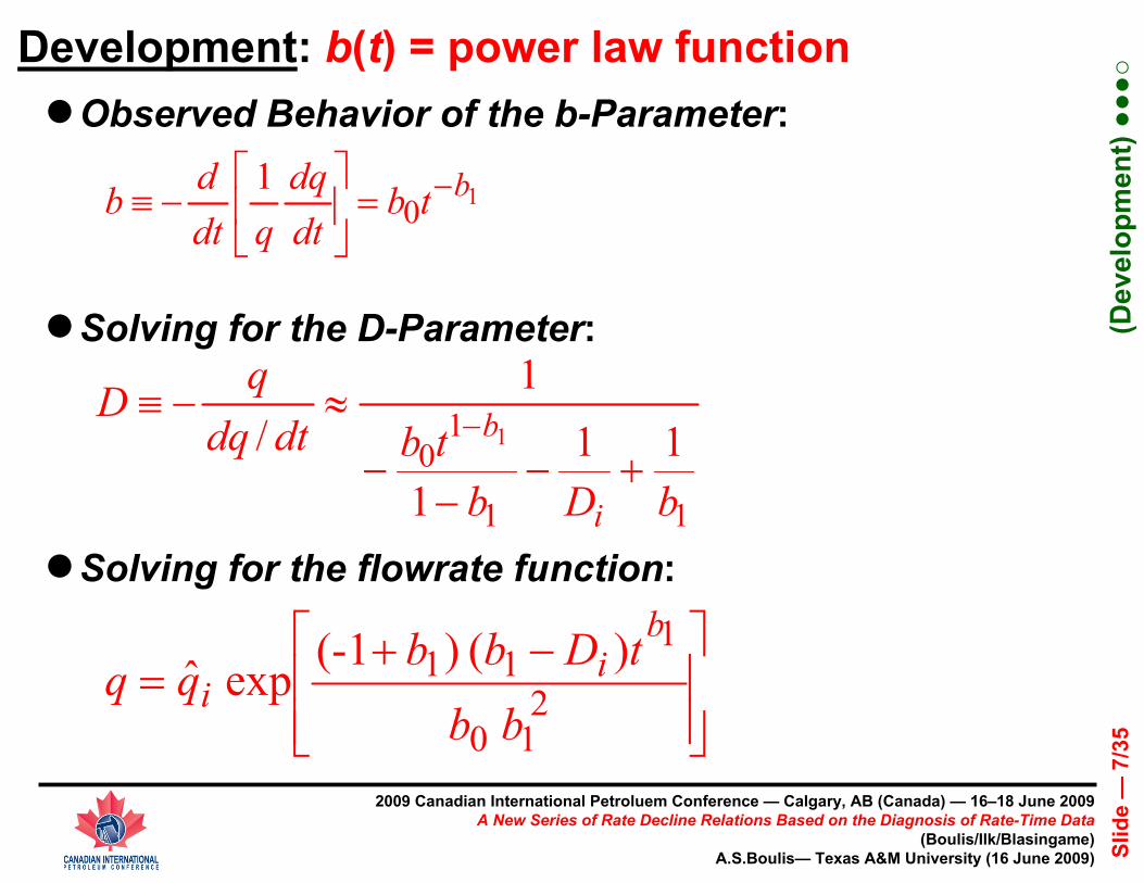
● b(t) = power-law function
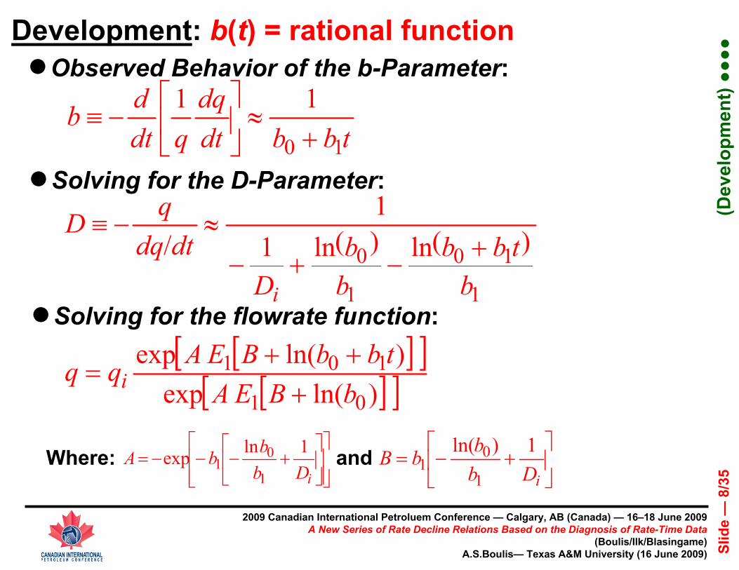
● b(t) = rational function
The corresponding rate decline relation for each case is obtained by solving the differential equation associated with the selected functional for the b-parameter. The complete derivation for each case is documented. We demonstrate each rate decline relation by application to various numerical simulation cases (for gas), as well as for field data obtained from tight/shale gas reservoirs.
Statement of the Problem
Decline curve analysis is one of the primary tools, which is practiced by the petroleum engineers to estimate reserves in oil and gas wells.
The widespread use of decline curve analysis is due to the simplicity of the exponential and hyperbolic rate-decline equations as introduced by Arps (Arps [1945]). Exponential and hyperbolic rate-decline equations are empirical relations based on observations of the well performance data and are only applicable for the boundary-dominated flow. These relations can be derived by using the so-called "loss-ratio" and the "derivative of the loss-ratio" definitions as proposed by Johnson and Bollens [1928] and later by Arps [1945].
Definition of the Loss-Ratio:
dtdqq
D /1
−≡ ............................................................................(1)
Derivative of the Loss-Ratio:
⎥⎦
⎤⎢⎣
⎡−≡⎥⎦
⎤⎢⎣⎡≡
dtdqq
dtd
Ddtdb
/1 ......................................................(2)
For reference, we present the derivations for the exponential and hyperbolic rate-decline cases in Appendix A. As mentioned earlier, exponential rate-decline case can be derived theoretically; for the case of constant compressibility liquid in a closed reservoir flowing at a constant wellbore flowing pressure during boundary-dominated flow conditions. To our knowledge there is no "theoretical" derivation for the hyperbolic rate-decline case. The hyperbolic rate-decline relation is obtained by assuming a constant value for the b-parameter in Eq. 2 and solving the associated differential equations.
In this work, we focus on the estimation of reserves in gas wells using only rate-time data. The common practice in the industry for reserves estimation is to use the hyperbolic rate-decline relation. However, our observations indicate that gas well performance behavior does not exhibit a constant b-parameter data trend when b-
PETROLEUM SOCIETY CANADIAN INSTITUTE OF MINING, METALLURGY & PETROLEUM
(Revision: 11 June 2009)
2
parameter is computed using rate-time data as dictated by Eq. 2. Despite this observation, it is still possible to use the hyperbolic rate-decline relation by using conservative values for the b-parameter (0<b<1) or using variations of hyperbolic rate decline relations (see Kupchenko et al [2008]).
The main issue is that the use of hyperbolic rate-decline relation could be applicable for conventional gas reservoirs. But, when production data from tight gas sand and shale gas wells are assessed using the hyperbolic rate-decline relation, the identification of a "reasonable" b-parameter is in fact really difficult due to the very long transient period. In practice we often observe b-parameter values higher than 1.0 — particularly, to the onset of true boundary-dominated flow. This situation results in the over-estimation of reserves by errors more than one hundred percent (see the recent study by Rushing et al [2007] on assessing the validity of using Arps' hyperbolic rate-decline relation).
There are also other methodologies which require flowing bottom-hole pressure data in addition to flowrate data for analyzing well performance to estimate reservoir properties and obtain gas-in-place. These methodologies are classified as the "modern decline analysis (decline type curves)" or "rate-transient analysis" techniques and they are based on the analytical solutions for several well/reservoir configurations (see Fetkovich [1980], Palacio and Blasingame [1993], Doublet et al [1994], Agarwal [1998], and Amini et al [2007] for details). Although, using "modern decline analysis" is more favorable, the flowing bottomhole pressure data may not available for every case and also for complex well/reservoir configurations (e.g., horizontal wells with multiple transverse fractures) the analytical solution may not be available. Under these circumstances the need for a practical method in addition to hyperbolic rate-decline is obvious to estimate reserves in tight gas sand and shale gas reservoirs. In this work, we propose to model the computed b-parameter trend from rate-time data according to Eq. 2 using several (continuous) functions. The solution of each corresponding differential equation yields the "empirical" rate-decline relation for each case and we test the performance of each rate-decline relation using simulated data and field data obtained from tight gas and shale gas wells.
Objectives
We state the following objectives for this work:
● To prove that the b-parameter is not constant (contrary to the hyperbolic rate-decline relation) but changes as a function of time.
● To provide a diagnostic understanding of the b-parameter (i.e., the behavior of the computed b-parameter data trend for several different cases).
● To propose a series of new rate-decline relations based on the characterization of the computed b-parameter trend.
● To demonstrate the applicability of the new rate-decline relations using both synthetic and field data.
We will next present a brief literature review on estimating the gas reserves using production data for completeness.
Literature Review
Analysis of production data can be categorized into the following: empirical methods and semi-analytical/analytical methods. In this section we will only discuss the empirical methods which make use of rate-time data to estimate gas reserves. The definition of the "loss-ratio" by Johnson and Bollens [1928] and later by Arps [1945] lays the foundation for the traditional decline curve analysis (i.e., empirical exponential and hyperbolic rate-decline relations). Arps suggested that the values for the b-parameter should fall between zero and one for the hyperbolic rate-decline relation but did not discuss the possibility of the value of the b-parameter for greater than one. Fetkovich et al (Fetkovich et al [1996]) discussed the relationships
between the b-parameter and various kinds of reservoir heterogeneities and drive mechanisms. However, the work by Fetkovich et al did not indicate a b-parameter value greater than one.
As mentioned earlier for unconventional gas reservoirs the value of the b-parameter could exceed one when hyperbolic rate-decline relation is applied. Maley (Maley [1985]) investigated the application of traditional decline curve analysis to tight gas reservoirs and documented cases from the Lower Cotton Valley tight gas sands with b-parameter values greater than one. In a recent study by Rushing et al (Rushing et al [2007]), it was indicated that the value of the b-parameter would generally fall between 0.5 and 1 for various reservoir and hydraulic fracture heterogeneities. It was also observed that the values of the b-parameter greater than one indicated transient or transitional flow rather than true boundary-dominated flow regime. Kupchenko et al (Kupchenko et al [2008]) discussed the application of a piecewise hyperbolic rate-decline relation to take the transient/transitional flow regimes into account and to prevent the over-estimation of reserves.
Recently Ilk et al (Ilk et al [2008a] and Ilk et al [2008b]) introduced the "power-law exponential" rate-decline model to estimate gas reserves. The basis of this model is to compute the D-parameter according to Eq. 1 and to model the computed D-parameter trend with a power-law equation with a constant at late times. The work by Mattar et al (Mattar et al [2008]) considered the application of the power-law exponential rate-decline model to shale gas wells. The results verified that not only the power-law exponential rate-decline model was very flexible enough to match transient, transition, and boundary-dominated flow data, but also it yielded consistent and reasonable reserves estimates. To our knowledge, this is a new attempt to model/characterize the loss-ratio and consequently the derivative of the loss-ratio with a continuous function rather than a constant. In addition to the work by Ilk et al, Valko (Valko [2008]) presented another form of power-law exponential model to forecast the production of unconventional gas reservoirs.
Development of New Series of Rate-Decline Relations
As mentioned earlier our primary objective in this work is to characterize the computed b-parameter trend and develop the corresponding the rate-decline relation according to each b-parameter model. In addition to constant b-parameter model — yielding the hyperbolic rate-decline relation — we propose three "continuous" functions to model the b-parameter trend. Our rationale behind developing various models is that we believe that only one model for the b-parameter is not enough to characterize the b-parameter for different conditions (e.g. different well/reservoir configurations). We note that the models we are proposing are empirical based on our observations of rate-time data.
The models for characterizing the b-parameter are:
● b(t)=b ("constant")
● b(t)=b0 exp[-b1 t] ("exponential")
● b(t)=b0 t -b1 ("power-law")
● b(t)=1/(b0 + b1 t) ("rational")
We derive the corresponding rate-decline relation associated with each model in Appendix A. For orientation, we present the rate-decline relations for each model as follows:
● b(t)=b (this yields the hyperbolic rate-decline relation.)
bi
i
tbDq
q /1)1( += .........................................................................(3)
● b(t)=b0 exp[-b1 t]
)01/(1
)01/(1011 ]))exp[1(]exp[( iDbbiDiDbbiD
ii btbDbtbbqq ++−+−+=...................................................................................................(4)
3
● b(t)= b0 t -b1
⎥⎥⎦
⎤
⎢⎢⎣
⎡ −−= 2
10
111 )()1(expbb
tDbbqqb
ii
................................................... (5)
● b(t)= 1/(b0 + b1 t)
⎥⎥⎦
⎤
⎢⎢⎣
⎡⎥⎦
⎤⎢⎣
⎡⎥⎦
⎤⎢⎣
⎡−−
⎥⎥⎦
⎤
⎢⎢⎣
⎡⎥⎦
⎤⎢⎣
⎡++−⎥
⎦
⎤⎢⎣
⎡−−
=
ii
i
ii
ii
DbE
Dbb
tbbbDbE
Dbb
qq11]ln[expexp
]ln[]ln[11]ln[expexp
0
1000
................................................................................................... (6)
In the equations above, b, b0, b1 are model parameters defined in each b-parameter model and Di, qi are the model parameters obtained from the solution of the corresponding differential equation for the rate function. We present the application and performance of each model in the next sections. We note the performance of each model can vary according to different well performance data. Therefore, it is our contention that all the proposed models should be applied at the same time. We also develop a step by step procedure for the application of the models. The procedure is given as:
1. Collect rate-time data.
2. Carefully edit the spurious data from the dataset.
3. Compute the D- and b-parameters by numerical differentiation according to Eqs. 1 and 2. We use the "Bourdet algorithm" (Bourdet [1989]) for numerical differentiation.
4. We also compute the D- and b-parameters by using rate-cumulative data according to the equations given below.
dQdq
D−≡
1 .............................................................................. (7)
⎥⎦⎤
⎢⎣⎡≡
DdQdqb 1 ......................................................................... (8)
5. Plot the "q-D-b" data and apply each b-parameter model to data set. We do not recommend a statistical approach (i.e., regression) to find the model parameters. Instead, we visually obtain the optimum matches for each model.
6. Compute the cumulative production as depicted by the model (this is done numerically for the proposed models) and forecast the production.
Validation of the New Rate-Decline Relations
In this section, as a mechanism for validation, we validate our proposed models for the b-parameter by making use of data sets generated by numerical simulation. We note that we use different reservoir configurations and reservoir fluid characteristics for our simulations.
Case 1: Horizontal Gas Well with Multiple Transverse Fractures (SPE 119897 Data)
This case considers a horizontal gas well having multiple transverse fractures (see Fig. 1 for rate and cumulative gas production versus time). The original data was earlier analyzed using the "power-law exponential" rate-decline model in the work by Mattar et al (Mattar et al [2008]). The model parameters and reservoir/fluid properties are provided in Table 1. It should be noted that this well is producing in a (bounded) rectangular reservoir and boundary effects are observed during late times of the production.
We start by applying the hyperbolic rate-decline relation to data (Arps' equation, b=constant model). But, before the application we emphasize the end-point effects caused by the numerical differen-tiation algorithm at late times — therefore, the end-point effects
should not be seen as a feature exhibited by data. We also note that the computed b-parameter data trend exhibits a declining behavior (as opposed to constant) and the computed D-parameter trend exhibits a straight line behavior (on log-log scale). The gas-in-place value in the simulation was 2.67 BSCF.
Our objective is not to find the "best-fit" according to each model. But, rather we use the three models in conjunction and force the same maximum cumulative production value for each case. For the hyperbolic rate-decline case we usually set the b value to an average value of the data trend (for this specific case, this value is set to 0.99 as depicted by data trend at late times).
For this case we set b=0.99, this gives us a fair match with the rate data and the hyperbolic rate-decline relation. Fig. 2 presents the q-D-b plot for the constant b case. However, the reserves are estimated to be 6.44 BSCF (nearly the 2.5 times of the original gas-in-place value). Our next task is to apply the exponential b-parameter trend to the computed b-parameter data.
The exponential b-parameter model can be more useful than the constant b model as the model indicates that at late times the decline trend is exponential. In fact it might be reasonable to assume to use an exponential decline when boundary-dominated flow regime is reached. The issue with the exponential b-parameter model is that at early/middle times, this relation is not sufficient to model transient/transitional flow. Therefore, the match of the rate data model with the exponential b-parameter model may not be adequate for all cases. Fig. 3 presents the q-D-b plot for the exponential b-parameter model case. We note the early time data are not modeled by the relation. However, the overall match of the rate data with the model is good and the reserves estimate is consistent with the gas-in-place input (Gp,max=2.67 BSCF).
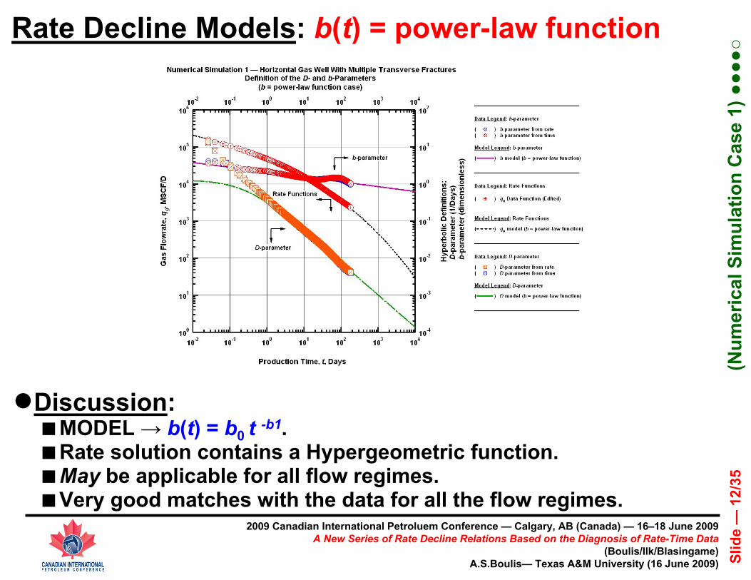
Our next step is to apply the power-law b-parameter model. The computed b-parameter data trend indicates a straight line behavior on the log-log scale (see the q-D-b plot, Fig. 4). As a result, the power-law b-parameter model should be a good candidate for estimating reserves in this case. We match the computed b-parameter data with the power-law model and observe a very good match. Consequently, D-parameter data and rate data matches are excellent (except for the early and late times — end point effects). The reserves estimate for this case is same with the exponential b-parameter model case (Gp,max=2.67 BSCF).
Finally we apply the rational b-parameter model to the computed b-parameter data trend. The rational b-parameter model is similar to the exponential b-parameter model in terms of modeling the b-parameter data (i.e., constant b at early times followed by a decline). We also note that the declining part of the b-parameter data trend can easily be modeled by the exponential and rational models. However, these models can not capture the early-time part of the data due to their nature. It can also be mentioned that the rational b-parameter model is more flexible than the exponential b-parameter model. For this case, we have a fair match of the computed b-parameter data trend with the model. The matches of D-parameter and rate data with the model are also similar to the exponential b-parameter case. Fig. 5 illustrates the application of the rational b-parameter model for this case. Again we obtain the same value for the reserves using the rational b-parameter model (see Figs. 6 and 7 for the production forecast, Gp,max=2.67 BSCF).
Case 2: Horizontal Gas Well
In this case we consider a horizontal gas well. We generate the synthetic rate performance using a numerical simulator. The model parameters and reservoir/fluid properties are provided in Table 2. It should be noted that this well is producing in a (bounded) rectangular reservoir and boundary effects are observed during late times of the production. Fig. 8 presents the summary history plot for this case (rate and cumulative gas production versus time). A visual inspection of the data suggests that boundary-dominated flow has

4
been established (i.e., straight line rate data behavior at late times on semi-log scale).
Before applying the proposed models to the data set, we inspect the computed b-parameter data trend. In this case the computed b-parameter data indicates a different behavior — at very early times b-parameter data trend exhibits an increasing trend then starts to decline and later stabilizes, then again shows a decreasing trend and finally stabilizes during complete boundary-dominated flow regime (end-point effects are not taken into account). We attribute these changes to the various flow regimes encountered in the case of a horizontal well.
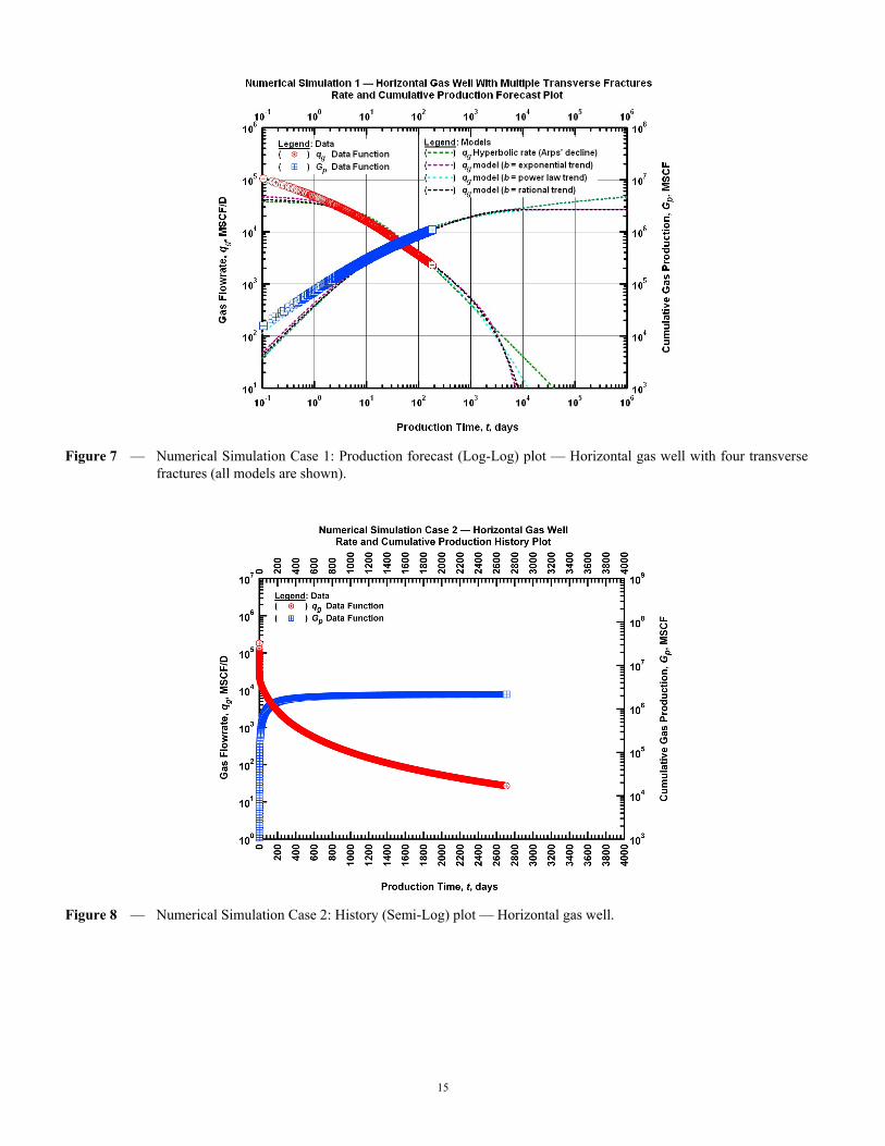
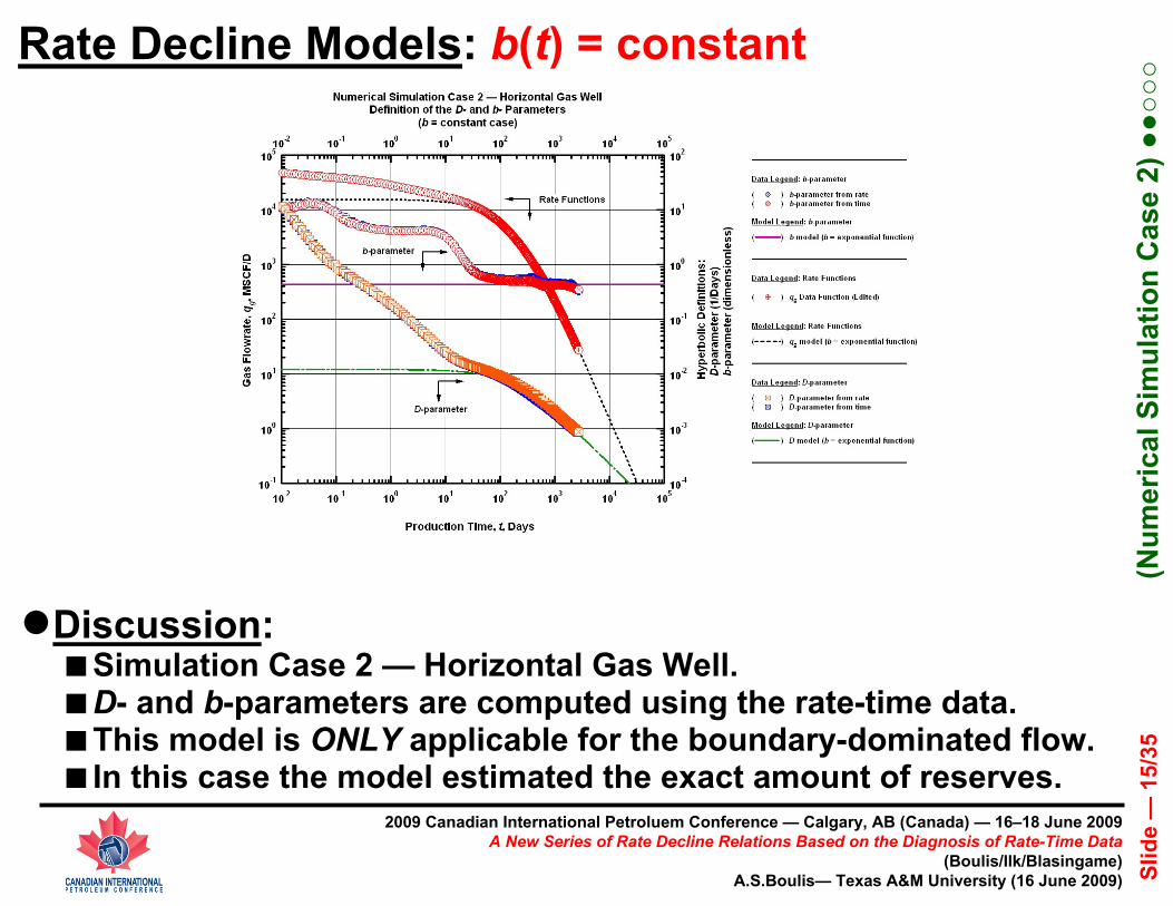
At late times the computed b-parameter data trend stabilizes at approximately 0.4 (see Fig. 9). Therefore, we use this value in the application of the Arps' hyperbolic rate-decline relation (constant b-parameter case). It is apparent that there is a very good match for the boundary-dominated flow data with the hyperbolic rate-decline relation (after 100 days). The reserves estimate (Gp,max=2.25 BSCF) is consistent with the numerical simulator input value (G=2.25 BSCF). This case suggests that if the complete boundary-dominated flow regime is reached, then it is possible to estimate the reserves with the hyperbolic rate-decline relation by computing the b-parameter using rate-time data. On the other hand, we acknowledge that this is a special case and for most of the unconventional gas reservoir applications it is very difficult to identify the onset of the boundary-dominated flow regime.
Next, we apply the exponential b-parameter model to the data set. We use the stabilized b-parameter value (approximately 0.4) for the b0 model parameter which actually dominates the early/middle time behavior. At late times the b1 model parameter starts to dominate and this defines the decline behavior of the model. Fig. 10 presents our matches for the exponential b-parameter model case with the data. We note that exponential b-parameter model performs slightly better than the Arps' hyperbolic rate-decline relation in terms of matching the rate data. The reserves estimate is found to be the same with the gas-in-place input value (Gp,max=2.25 BSCF).
For the power-law b-parameter model, the computed b-parameter data trend implies that this model should not be applicable for this case. This situation clearly explains why we need more than one b-parameter models — each proposed model might work better for a particular case. Our strategy for applying the power-law b-parameter model is to find an average straight line which passes through the computed b-parameter data trend. By doing so, we obtain the matches in Fig. 11 and our estimate for the reserves is the same with the previous cases (Gp,max=2.25 BSCF). We note that the match of the rate data with the power-law b-parameter model is good (perhaps the best among all models) confirming our strategy to use an average b-parameter data.
Finally we apply the rational b-parameter model. Our expectations for this case are the same with the exponential b-parameter model. Similarly we obtain the same matches of the data with the rational b-parameter model as in the case of the exponential b-parameter model (see Fig. 12 for the matches). Production forecast plots (Figs. 13 and 14) suggest the same reserves estimate as with the other models. Our concluding remarks for this case are as follows. None of the models can model the transient/transitional part of the computed b-parameter data trend successfully. This causes a mismatch of the models with the computed b-parameter data but since the boundary-dominated flow regime is established, the reserves estimate can be obtained. For this case the best match of the rate data can be achieved by using an average "straight-line" trend (using the power-law b-parameter model) for the computed b-parameter data.
Field Case Demonstration Examples
The purpose of using field cases is to demonstrate the application of the new rate-decline relations. We have validated the new rate-decline relations to a certain extent by using the numerical simulation examples earlier. Our next step is to use the new rate-decline
relations in estimating the reserves for specific field data cases. In this paper we will show the application specifically for unconventional gas reservoirs. We have two examples — fractured gas well in a tight gas sand reservoir and shale gas well.
Field Case 1: Fractured Gas Well in a Tight Gas Sand Reservoir (Ilk et al [2008c])
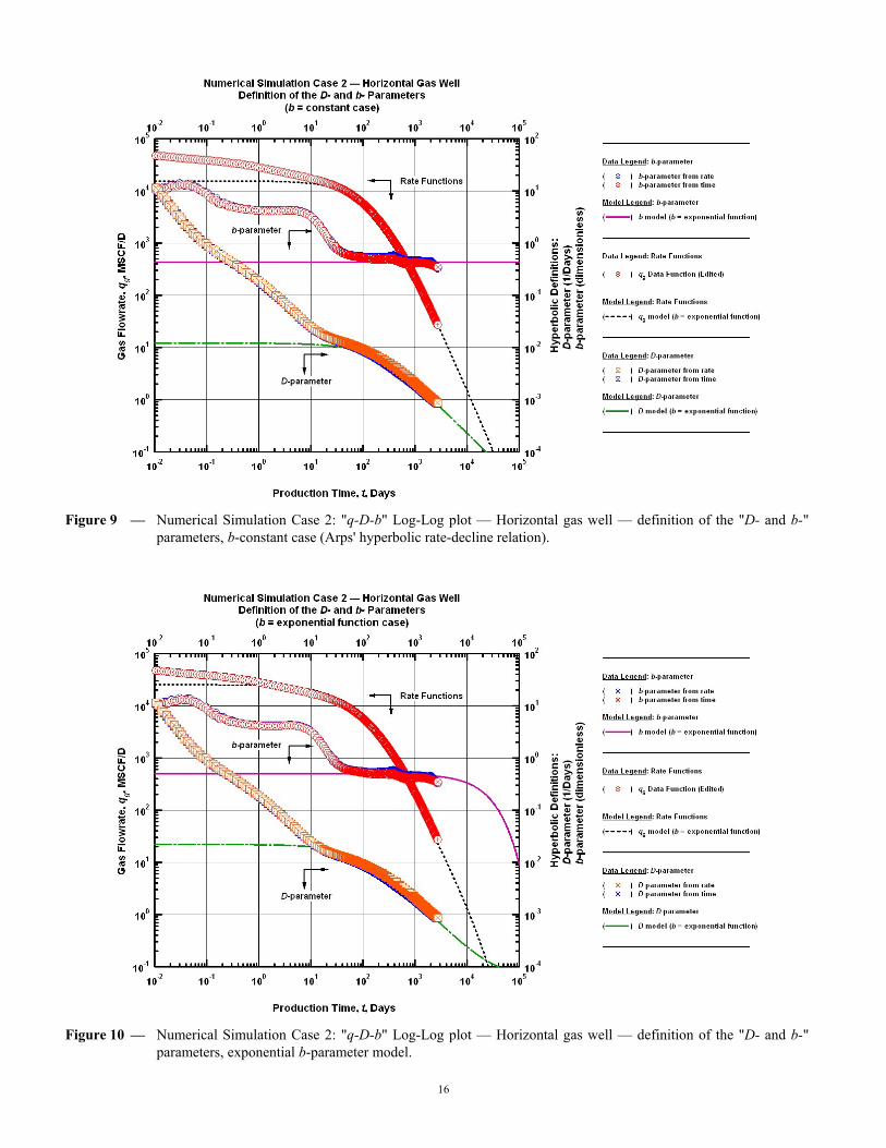
Our first example is taken from the work by Ilk et al (Ilk et al [2008c]). This is a hydraulically fractured gas well producing in a tight gas sand reservoir (this well corresponds to well LWF1 in the work by Ilk et al). Fig. 15 presents the summary history plot for this case. Daily surface pressure and flowrate data are available for this well. Data quality seems good in general except for the liquid loading effects reflected in the flowrate data. The pressure data are not shown in this work. Model based analysis (ref. Ilk et al [2008c]) yielded 3.0 BSCF for the contacted gas-in-place estimate. In this case we will try to find the same value using the new rate-decline relations as obtained by the model based analysis.
We follow our step by step procedure for the application of the rate-decline relations. First of all, we edit/delete the spurious rate data prior to numerical differentiation. Once editing is complete, the numerical differentiation can be performed.
Fig. 16 illustrates the application of the Arps' rate-decline equation to this case. We set the b-parameter value to 0.9 and obtain the best matches. The rationale for the b-parameter value equals to 0.9 is that the computed b-parameter trend stabilizes at 0.9 at late times. Using this value, we obtain the reserves estimate to be 8.4 BSCF for this case. This is clearly an over-estimate and from the data it can be seen that the complete boundary-dominated flow regime has not been established yet.
In the next attempt, we use the exponential b-parameter model. In some sense, the exponential b-parameter model is a way to constrain the Arps' hyperbolic rate decline relation by introducing the exponential decline at late times. We use the same value for the model parameter, b0, as in the case of the hyperbolic rate-decline relation (in other words we set b0=b). We obtain the optimum match by changing the value of the remaining model parameters. Fig. 17 presents our matches for this case. The reserves estimate is consistent with the model based analysis (Gp,max=3.0 BSCF).
The computed b-parameter data trend indicates a power-law behavior. Therefore, we expect that for this case power-law b-parameter model should perform very well. Fig. 18 presents the "q-D-b" plot for this case. As expected we obtain outstanding matches of all the data with the power-law b-parameter model and its associated relations. In particular, the match of the rate data with the model is excellent. We note that we obtain the same reserves estimate as with the other models using the power-law b-parameter model (Gp,max=3.0 BSCF).
Finally we apply the rational b-parameter model to the data set. We believe the rational b-parameter model is the most flexible among the proposed models in terms of modeling the computed b-parameter data trend. We present the model matches with the data in Fig. 19. We observe extraordinary matches of the data with the models. The data are matched to the model across all flow regimes. The reserves estimate is found to be 3.0 BSCF. Figs. 20 and 21 present the production forecast for this case.
Field Case 2: Shale Gas Well (Mattar et al [2008])
The second example includes the monthly production data acquired from a shale gas well (Barnett Shale). The production data was earlier analyzed in the work by Mattar et al [2008] using the "power-law exponential" rate-decline model (Ilk et al [2008a] and [2008b]). Our objective in this work is to get a consistent reserves estimate with the "power-law exponential" model using the new rate-decline

5
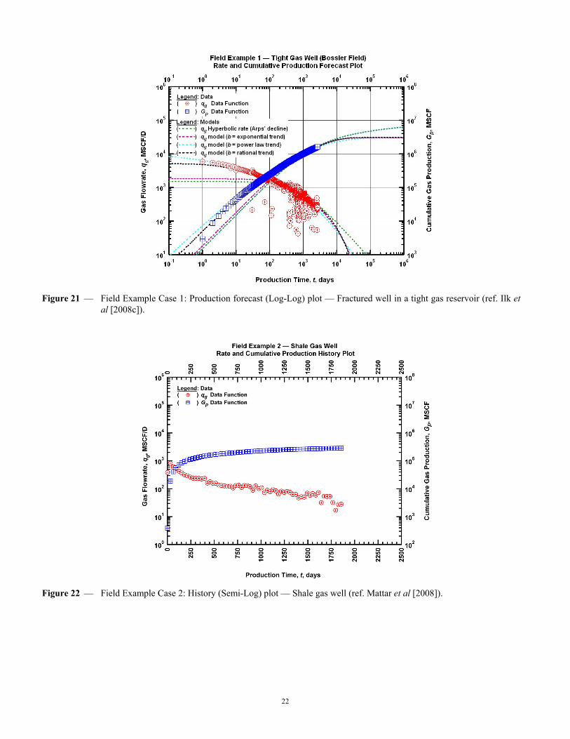
relations. As mentioned before, almost 6.5 years of monthly production data are available via public records (see Fig. 22). For this case we note that boundary-dominated flow regime has been established by visual inspection.
We first apply the hyperbolic rate-decline relation by setting b equal to 0.9 as suggested by the computed b-parameter data trend. The matches in Fig. 23 are good but we note that most of the transient/transitional data are missing. The reserves estimate by the hyperbolic rate-decline relation over-estimates the reserves estimate using the "power-law exponential" rate-decline model (Gp,max=0.33 BSCF).
We use the same rationale in the exponential b-parameter model but as mentioned earlier the exponential b-parameter model constrains the reserves estimate. Fig. 24 presents the matches of the data with exponential b-parameter model and its associated relations. We can conclude from Fig. 24 that all the matches are good and the reserves estimate is consistent (Gp,max=0.335 BSCF). However, it should be noted that most of the transient/transitional data are missing — preventing the actual performance of the model.
Similarly for the power-law b-parameter model, we obtain good matches (see Fig. 25). In fact, the computed b-parameter data trend is not clear enough to exhibit an obvious behavior. Nevertheless, we can obtain consistent results by using all the proposed models in conjunction with each other. For example, the power-law b-parameter model is applied and forced to yield the same reserves estimate with the other models. The matches in Fig. 25 confirm the methodology and reserves estimate (Gp,max=0.335 BSCF).
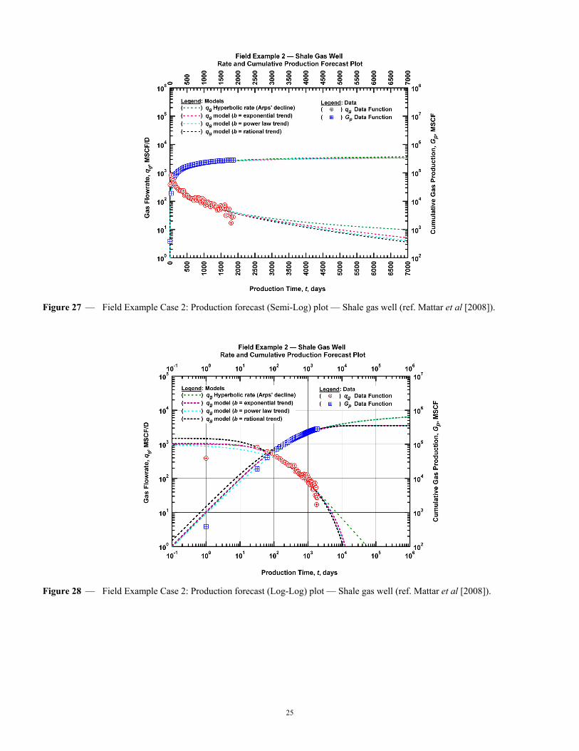
Finally, we apply the rational b-parameter model for this case. Fig. 26 presents the results — we can conclude that the best matches of the data with the model are obtained for this case. We believe this is due to the flexibility of the rational b-parameter model. We note that all the data are matched across all flow regimes. We obtain the same reserves estimate as with the other models and this result is consistent with the result from the work by Mattar et al. Figs 27 and 28 present the production forecast for this well using all the models.
Summary and Conclusions
We derive the following summary and conclusions from this work.
Summary
In this work we have proposed the following models for characterizing the b-parameter in addition to the Arps' hyperbolic rate decline relation (constant b-parameter case):
● b(t) = constant (Arps' hyperbolic rate-decline relation)
● b(t) = exponential function
● b(t) = power-law function
● b(t) = rational function
The proposed functions (models) are empirical and based on our observations. We derive the corresponding rate-decline relation for each b-parameter model by using Eqs. 1 and 2 and solving the differential equation related with each b-parameter model. We apply the new rate-decline models to two numerical simulation cases, one tight gas sand reservoir case, and one shale gas reservoir case. Our results indicate that the new rate-decline models could be a useful addition to reserve estimate methods using only rate-time data.
Conclusions
1. The continuous evaluation/interpretation of the computed b-parameter data trend enhances the diagnostic understanding of the b-parameter. The behavior of the computed b-parameter data trend varies for different well/reservoir configurations (see numerical simulation cases in this work for clarity). Therefore, new rate-decline relations are required to obtain better estimates for reserves.
2. The performance of the new rate-decline relations corres-ponding to each b-parameter model:
● b(t) = constant: This case corresponds to classical Arps' hyperbolic relation. Our experience so far has suggested that the computed b-parameter trend is not constant. Also, this relation is only applicable for the boundary-dominated flow regime. If the data do not exhibit boundary-dominated flow, this relation significantly over-estimates the reserves.
● b(t) = exponential function: This model is a constrained form of the constant b-parameter model. The exponential function indicates that the b-parameter is constant for early and middle times, but exhibits an exponential decline for late times (boundary-dominated flow). This is consistent with the boundary-dominated flow regime behavior, but transient part of the rate data can not be represented with this model. This model also gives conservative reserve estimates.
● b(t) = power-law function: The power-law function models the computed b-parameter trend as a straight line on log-log scale. For some cases — for example, tight gas example in this work — we have observed that the computed b-parameter trend exhibits a power-law behavior. For those cases the matches are outstanding and the reserves estimates are reliable.
● b(t) = rational function: We believe that the rational function for the b-parameter is the most flexible model among all the proposed models. Early time behavior is dominated by a constant, middle and late time behavior is dominated by the other model parameters causing a decline behavior. With this model, it is possible to match the computed D-parameter data trend all across. Thus, the match of the rate data with the rate-decline relation can often be outstanding across all flow regimes. However, the rate-decline relation is tedious and it includes a special function (i.e., the exponential integral) to be evaluated — on the other hand, this rate-decline relation can easily be programmed in a spreadsheet.
3. We emphasize that we do not favor a specific b-parameter model proposed in this work. We believe that each model has advantages and disadvantages — and the performance of the models can vary under different conditions. Under these circumstances we suggest the use of all the b-parameter models in conjunction to yield better resolution and to decrease the uncertainty in reserves estimates.
4. We have also observed in some cases that the computed b-parameter trend varies according to the well/reservoir configuration (i.e., different flow regimes). Numerical simulation cases 1 and 2 are an example of this situation. As mentioned earlier, the applicability of the models can change depending on the particular case, but we have also shown that an average representation of the computed b-parameter with the proposed models might also yield consistent results and reasonable rate data matches. However, this condition needs to be further investigated.
Recommendations
1. For better understanding of the character of the computed b-parameter data, more models in addition to the ones proposed in this work need to be developed.
2. These models need to be applied to more cases including a variety of field data. Also, more numerical simulation cases for complex well/reservoir configurations need to be investigated.

6
3. Comparison with the analytical solutions can also be performed to validate the proposed models from a theoretical stand point.
Nomenclature
Variables:
2F1(x) = Hypergeometric series (Gauss' hypergeometric functions)
A = Drainage area, acres b = Arps' decline exponent b0 = model parameter b1 = model parameter cf = Formation compressibility, psi-1 D = Decline parameter defined by Eq. 1 Di = Initial decline parameter (t=0) Ei(x) = Exponential integral Gp = Cumulative gas production, MSCF Gp,max = Maximum gas production, MSCF q = Gas production rate, MSCF/D qi = Initial Gas production rate, MSCF/D or STB/D h = Net Pay thickness, ft k = Average reservoir permeability, md Lh = Horizontal well length, ft pwf = Average reservoir pressure, psia re = Reservoir drainage radius, ft rw = Wellbore radius, ft s = Skin factor, dimensionless Sg = Gas saturation, fraction t = Time, days T = Reservoir temperature, °F wf = Fracture width, inches zw = Position of the horizontal well, ft
Dimensionless Variables:
FcD = Dimensionless fracture conductivity
Greek Symbols:
γg = Reservoir gas specific gravity (air = 1) φ = Porosity, fraction
Subscripts:
i = Integral function or initial value
SI Metric Conversion Factors cp × 1.0 E-03 = Pa·s ft × 3.048 E-01 = m md × 9.869 233 E-04 = μm2 psi × 6.894 757 E+00 = kPa bbl × 1.589 873 E-01 = m3
*Conversion factor is exact.
References
Abramowitz, M. and Stegun, I.A. 1972. Handbook of Mathematical Functions. New York: Dover. Agarwal, R.G., Gardner, D.C., Kleinsteiber, S.W. and Fussell, D.D. 1999. Analyzing Well Production Data Using Combined Type-Curve and Decline-Curve Analysis Concepts. SPEREE. 2 (5): 478-486. Amini, S., Ilk, D., and Blasingame, T.A. 2007. Evaluation of the Elliptical Flow Period for Hydraulically-Fractured Wells in Tight Gas Sands — Theoretical Aspects and Practical Considerations. Paper SPE 106308 presented at the SPE Hydraulic Fracturing Technology Conference held in College Station, Texas, U.S.A., 29–31 January. Arps J.J. 1945. Analysis of Decline Curves. Trans. AIME: 160, 228-247. Blasingame, T.A. and Rushing, J.A. 2005. A Production-Based Method for Direct Estimation of Gas-in-place and Reserves. SPE paper 98042 presented at the SPE Eastern Regional Meeting, Morgantown, West Virginia. 14-16 September.
Bourdet, D., Ayoub, J.A., and Pirad, Y.M. 1989. Use of Pressure Derivative in Well-Test Interpretation. SPEFE. 4 (2): 293-302. Doublet, L.E., Pande, P.K, McCollum, T.J., and Blasingame, T.A. 1994. Decline Curve Analysis Using Type Curves—Analysis of Oil Well Production Data Using Material Balance Time: Application to Field Cases. Paper SPE 28688 presented at the International Petroleum Conference and Exhibition of Mexico, Veracruz, Mexico, 10-13 October. Fetkovich, M.J. 1980. Decline Curve Analysis Using Type Curves. JPT. 32 (6): 1065-1077. Fetkovich, M.J., Fetkovich, E.J., and Fetkovich, M.D. 1996. Useful Concepts for Decline-Curve Forecasting, Reserve Estimation and Analysis. SPERE. 11 (1): 13-22. Gradshteyn, I.S., and Ryzhik, I.M. 1996. Table of Integrals, Series, and Products. San Diego: Academic Press. Ilk, D., Rushing, J.A., and Blasingame, T.A. 2008a. Estimating Reserves Using the Arps Hyperbolic Rate-Time Relation — Theory, Practice and Pitfalls. Paper CIM 2008-108 presented at the 59th Annual Technical Meeting of the Petroleum Society, Calgary, Alberta, Canada, 17-19 June. (in preparation) Ilk, D., Perego, A.D., Rushing, J.A., and Blasingame, T.A. 2008b. Exponential vs. Hyperbolic Decline in Tight Gas Sands — Understanding the Origin and Implications for Reserve Estimates Using Arps' Decline Curves. Paper SPE 116731 presented at the SPE Annual Technical Conference and Exhibition, Denver, Colorado, 21-24 September. Ilk, D., Perego, A.D., Rushing, J.A., and Blasingame, T.A. 2008c. Integrating Multiple Production Analysis Techniques To Assess Tight Gas Sand Reserves: Defining a New Paradigm for Industry Best Practices. Paper SPE 114947 presented at the SPE Gas Technology Symposium, Calgary, Alberta, Canada, 17-19 June. Johnson, R.H. and Bollens, A.L. 1927. The Loss Ratio Method of Extrapolating Oil Well Decline Curves. Trans. AIME 77: 771. Kupchenko, C.L., Gault, B.W., and Mattar, L. 2008. Tight Gas Production Performance Using Decline Curves. Paper SPE 114991 presented at the SPE Gas Technology Symposium, Calgary, Alberta, Canada, 17-19 June. Maley, S. 1985. The Use of Conventional Decline Curve Analysis in Tight Gas Sands. Paper SPE 13898 presented at the SPE Low Permeability Gas Reservoirs Symposium, Denver, CO, May 19-22. Mathematica. 2007. http://www.wolfram.com Mattar, L., Gault, B.W., Morad, K., Clarkson, C.R., Freeman, C.M., Ilk, D., and Blasingame, T.A. 2008. Production Analysis and Forecasting of Shale Gas Reservoirs: Case History-Based Approach. Paper SPE 119897 presented at the SPE Shale Gas Production Conference, Fort Worth, TX, 16-18 November. Palacio, J.C., and Blasingame, T.A. 1993. Decline Curve Analysis With Type Curves — Analysis of Gas Well Production Data. Paper SPE 25909 presented at the SPE Rocky Mountain Regional/Low Permeability Reservoirs Symposium, Denver, CO., 12-14 April. Rushing, J.A., Perego, A.D., Sullivan, R.B., and Blasingame, T.A. 2007. Estimating Reserves in Tight Gas Sands at HP/HT Reservoir Conditions: Use and Misuse of an Arps Decline Curve Methodology. Paper SPE 109625 presented at the 2007 Annual SPE Technical Conference and Exhibition, Anaheim, CA., 11-14 November. Valko, P.P. 2009. Assigning Value to Stimulation in the Barnett Shale: A Simultaneous Analysis of 7000 Plus Production Histories and Well Completion Records. Paper SPE 119369 presented at the SPE Hydraulic Fracturing Technology Conference, Woodlands, TX, January 19-21.
7
Appendix A — Derivation of the Rate Decline Relations
The derivation of the Arps hyperbolic rate relation (Arps [1945]) is provided earlier in the work by Blasingame and Rushing [2006]. This derivation is provided for the purpose of orienting the analyst in the application of the Arps hyperbolic rate decline relation. Although there is no theoretical basis to force the "b-parameter" in the range between 0 and 1 (0<b<1), we suggest the use of the hyperbolic rate relation as a starting point for "modern" methods to correlate and extrapolate rate performance behavior by limiting the b-parameter between 0 and 1.
Arps defined the so-called "loss-ratio" and the "derivative of the loss-ratio" functions as:
Definition of the Loss-Ratio:
dtdqq
D /1
−≡ ....................................................................... (A-1)
Derivative of the Loss-Ratio:
⎥⎦
⎤⎢⎣
⎡−≡⎥⎦
⎤⎢⎣⎡≡
dtdqq
dtd
Ddtdb
/1 .................................................. (A-2)
As mentioned earlier, our primary objective in this work is to characterize the behavior of the "b-parameter" and consequently obtain the corresponding rate-time relation. In this appendix we derive the rate relations for the proposed characterizations for the "b-parameter".
Exponential Rate Decline Case (b=0)
This case corresponds to the special condition where the "b-parameter" is equal to zero. Using this condition we have
dtdqq
D /1
−= .......................................................................... (A-3)
Equation A-3 implies that the D-parameter is constant and can be defined as Di (i.e., initial decline). Consequently, Eq. A-3 becomes
iDdtdq
q−=
1 ............................................................................ (A-4)
Separation of variables yields
dtDq
dqi−= ............................................................................ (A-5)
Integrating Eq A-5, we obtain:
∫∫ −=
t
i
q
iq
dtDqdq
0
..................................................................... (A-6)
Completing the integration gives us the following result:
tDqq
ii
−≡⎥⎦
⎤⎢⎣
⎡ln ........................................................................ (A-7)
In order to solve for the rate function, we exponentiate and rearrange both sides, this yields the exponential rate decline relation:
)exp( tDqq ii −= ..................................................................... (A-8)
Hyperbolic Rate Decline Case (b=constant)
The starting point for this case is Eq. A-2 where we assume that the b-parameter is constant.
⎥⎦
⎤⎢⎣
⎡−≡
dtdqq
dtdb
/..................................................................... (A-9)
Separating the variables we have:
dtbdtdq
qd −=⎥⎦
⎤⎢⎣
⎡/
................................................................. (A-10)
Taking the indefinite integration yields
ctbdtdq
q−−=
/................................................................... (A-11)
where c is defined as the constant of integration. Recalling the definition of the loss-ratio (Eq. A-1):
cbtD
+=1 ............................................................................ (A-12)
The definition for the initial decline term states that Di is defined as t goes to zero (i.e., D ≈ Di, t → 0). By using this definition we obtain the value for the constant of integration.
cDi
=1 ................................................................................. (A-13)
Substituting the constant of integration in Eq. A-11 gives us:
iDtb
dtdqq 1/
−−= ................................................................ (A-14)
Taking the reciprocal of Eq. A-14 we have:
tbDD
Dbtdt
dqq i
i
i
+−=
−−=
11
111 .......................................... (A-15)
By integrating Eq. A-21 we have:
∫∫ +−=⎥
⎦
⎤⎢⎣
⎡=
t
ii
i
q
iq
dttbD
Dqqdq
q0
11ln1 ................................... (A-16)
To solve the integral in the right-hand-side of Eq A-16, a variable of substitution is defined as shown below:
)1 ;at and 1 ;0(at 1 tbDzttzttbDz ii +====+= ............... (A-17)
Therefore:
dzbD
dtdtbDdzi
i1or 1 =+= .............................................. (A-18)
By using the transformation, the right-hand-side of the equation becomes:
⎥⎥
⎦
⎤
⎢⎢
⎣
⎡+=
+−=
⎥⎦⎤
⎢⎣⎡−=
⎥⎦
⎤⎢⎣
⎡⎥⎦⎤
⎢⎣⎡−=
+−=
−
+
+
∫
∫
∫
bi
i
tibD
i
tibD
ii
t
ii
tbD
tbDb
dzz
Db
dzbDz
D
dttbD
DRHS
1
1
0
1
0
0
)1(ln
]1ln[1
11
11
11
............................................ (A-19)
Substituting the solution of the right-hand-side into Eq. A-16, we finally have:
⎥⎥
⎦
⎤
⎢⎢
⎣
⎡+=⎥
⎦
⎤⎢⎣
⎡ −b
ii
tbDqq
1
)1(lnln .................................................... (A-20)
Exponentiating the both sides of Eq. A-20, we have:
bi
itbD
1
)1(−
+= ................................................................. (A-21)
Solving for the rate term yields the hyperbolic rate decline relation:
bi
i
tbDq
q /1)1( += .................................................................. (A-22)

8
The special case for Eq. A-22 is defined when the b-parameter is equal to one. This condition refers to the "harmonic" rate-decline relation (as shown below).
)1( tDqq
i
i+
= ......................................................................... (A-23)
Characterization of the b-parameter — Derivation of the New Rate Decline Relations
● b(t)=b0 exp[-b1 t]
This case presents the derivation of the rate relation based on characterizing the b-parameter as an exponential function. We propose the following equation to model the b-parameter.
]exp[)( 10 tbbtb −= ............................................................... (A-24)
Recalling the definition of the derivative of the loss-ratio (Eq. A-2) and inserting Eq. A-24 for the b-parameter term, we have:
]exp[/ 10 tbbdtdq
qdtd
−=⎥⎦
⎤⎢⎣
⎡− .................................................. (A-25)
Separating the terms and integrating indefinitely yields:
∫∫ −=⎥⎦
⎤⎢⎣
⎡− dttbb
dtdqqd ]exp[/ 10 .......................................... (A-26)
Completing the integration we have:
cb
tbbdtdq
q+
−−=−
1
10 ]exp[/
................................................ (A-27)
Where c is defined as the constant of integration. Recalling the definition for the D-parameter, we have:
cb
tbbD
+−
−=1
10 ]exp[1 ......................................................... (A-28)
We set t=0 (D=Di) and solve for the constant of integration. This gives:
1
01bb
Dc
i+= ......................................................................... (A-29)
Substituting Eq. A-29 into Eq. A-27 we obtain:
1
0
1
10 1]exp[/ b
bDb
tbbdtdq
q
i++
−−=− ...................................... (A-30)
Taking the reciprocal of Eq. A-30 gives us:
⎥⎦
⎤⎢⎣
⎡++
−−
=−
1
0
1
10 1]exp[11
bb
Dbtbbdt
dqq
i
.................................. (A-31)
Separating the rate (q) and time (t) variables, we have:
⎥⎦
⎤⎢⎣
⎡++
−−
=−
1
0
1
10 1]exp[bb
Dbtbb
dtqdq
i
...................................... (A-32)
Taking the integral of both sides yields:
∫∫⎥⎦
⎤⎢⎣
⎡++
−−
=−
1
0
1
10 1]exp[bb
Dbtbb
dtqdq
i
................................ (A-33)
Completing the integration, we obtain:
ctbDbtbbDbb
Dq ii
i ])]exp[1(]exp[ln[]ln[ 101101
+−++
=− ........ (A-34)
Where c is defined as the integration constant. We use the following condition to find the integration constant, c.
0 , →= tqq i .................................................................... (A-35)
As t → 0, Eq. A-34 becomes:
cbDbb
Dq
i
ii ]ln[]ln[ 1
01 +=− .................................................. (A-36)
Solving for the integration constant, c, we obtain:
cb
qiDbbiD
i =+− )01/(
1
............................................................ (A-37)
Substituting Eq. A-37 into Eq. A-34 yields:
)01/(1
101101
])]exp[1(]exp[ln[]ln[iDbbiD
ii
i
i
bqtbDbtbb
DbbDq
+−+−+
+−
=
............................................................................................ (A-38)
Finally, rearranging Eq. A-38 for the rate term, we obtain the following relation for the case where the b-parameter is characterized as an exponential function:
)01/(1
)01/(1011 ])exp[1(]exp[( iDbbiDiDbbiD
ii btbDbtbbqq ++−+−+=
............................................................................................ (A-39)
Eq. A-39 can be represented in a simpler form as:
])exp[( DtCBAq −++= ...................................................... (A-40)
● b(t)=b0 t -b1
For this case we model the b-parameter trend as a power-law function. This formulation is given as:
10)( btbtb −= ........................................................................ (A-41)
Recalling the definition of the derivative of the loss-ratio (Eq. A-2) and inserting Eq. A-41 for the b-parameter term, we have:
10/btb
dtdqq
dtd −=⎥
⎦
⎤⎢⎣
⎡− .......................................................... (A-42)
Separating the terms and integrating indefinitely yields:
dttbdtdq
qd b∫∫ −=⎥⎦
⎤⎢⎣
⎡− 10/
................................................... (A-43)
Completing the integration we have:
cb
tbdtdq
q b+
−−=−
−
1
1101/
........................................................ (A-44)
Where c is defined as the integration constant. We obtain the value of c similarly as before.
1
11bD
ci
+−= ...................................................................... (A-45)
Substituting Eq. A-45 into Eq. A-44, we have:
11
110 111/ bDb
tbdtdq
q
i
b+−
−−=−
−............................................. (A-46)
Taking the reciprocal of both sides we obtain the following:
⎥⎥⎦
⎤
⎢⎢⎣
⎡−+
−
=−
11
110 111 bDb
tb
dtq
dq
i
b................................................... (A-47)
Separating and integrating yields:
∫∫⎥⎥⎦
⎤
⎢⎢⎣
⎡−+
−
=−
11
110 111 bDb
tb
dtq
dq
i
b............................................. (A-48)
The integration on the right-hand-side is performed using a symbolic computer language (Mathematica [2007]): The result is given as:
cDbb
tDbbbb
FtDb
Dbqi
bi
i
i
⎥⎥⎦
⎤
⎢⎢⎣
⎡
−−−+
−−=
−
))(1(,
111,1,
11]ln[
11
1110
1112
1
1
............................................................................................ (A-49)
Where c is defined as the integration constant and 2F1 is the hypergeometric function (Gradshteyn and Ryzhik [1980]). Solving for the integration constant (t=0), we obtain:
iqc = ................................................................................... (A-50)
9
For our purposes we perform a two-term series expansion for the hypergeometric function (2F1).
i
bi
i
bi
DbbtDbb
DbbtDbb
bbF 2
10
)11(11
11
1110
1112
)()1(1))(1(
,1
11,1,1
1 −− −−+≈
⎥⎥⎦
⎤
⎢⎢⎣
⎡
−−−+
−
............................................................................................. (A-51)
Inserting A-51 into Eq. A-49 and rearranging gives us the rate-decline relation for the power-law b-parameter case:
⎥⎥⎦
⎤
⎢⎢⎣
⎡ −−= 2
10
111 )()1(expbb
tDbbqqb
ii
............................................. (A-52)
We note that Eq. A-52 can be written in a general form as:
]exp[ CBtAq −= .................................................................. (A-53)
Where A, B, and C are constants.
● b(t)=1/(b0 + b1 t)
For this case we model the b-parameter trend as a rational function given by the following equation:
)/(1)( 10 tbbtb += ................................................................. (A-54)
Recalling the definition for the derivative of the loss-ratio (Eq. A-2), we have:
)/(1/ 10 tbbdtdq
qdtd
+=⎥⎦
⎤⎢⎣
⎡− .................................................... (A-55)
Separating and integrating yields:
∫∫ +=⎥
⎦
⎤⎢⎣
⎡−
)(/ 10 tbbdt
dtdqqd .................................................. (A-56)
Completing the integration of both sides, we obtain:
cb
tbbdtdq
q+
+=−
1
10 ]ln[/
...................................................... (A-57)
c is defined as the constant of integration. We obtain the value for the constant of integration by setting t=0.
cbb
Di+=
1
0]ln[1 .................................................................... (A-58)
1
0 ]ln[1bb
Dc
i−= .................................................................... (A-59)
Substituting Eq. A-59 into Eq. A-57, we have:
1
0
1
10 ]ln[1]ln[/ b
bDb
tbbdtdq
q
i−+
+=− ....................................... (A-60)
Separating and taking the reciprocal of both sides yields:
⎥⎦
⎤⎢⎣
⎡−+
+=−
1
0
1
10 ]ln[1]ln[/bb
Dbtbbdt
qdq
i.................................. (A-61)
Next we take the integral of both sides:
∫∫ ⎥⎦
⎤⎢⎣
⎡−+
+=−
1
0
1
10 ]ln[1]ln[/bb
Dbtbbdt
qdq
i............................ (A-62)
The integration on the right-hand-side is taken using a symbolical computer language (Mathematica [2007]). Completing the integ-ration, we have the following relation for the right-hand-side:
ctbbbDbE
DbbRHS
ii
i⎥⎦
⎤⎢⎣
⎡++−⎥
⎦
⎤⎢⎣
⎡−= ]ln[]ln[11]ln[exp 1000 ......... (A-63)
Where c is the integration constant, and Ei is the exponential integral function and defined as (Abramowitz and Stegun [1972]):
∫∞
−
−−=
z
i dtt
tzE ]exp[][ ........................................................... (A-64)
Solving for c, we have (t=0, q=qi):
⎥⎥⎦
⎤
⎢⎢⎣
⎡⎥⎦
⎤⎢⎣
⎡⎥⎦
⎤⎢⎣
⎡−−=
ii
ii D
bEDbbqc 11]ln[expexp 0 ................................. (A-65)
Substituting the value for c into the solution for the integration, we obtain the rate-decline relation for the rational b-parameter case:
⎥⎥⎦
⎤
⎢⎢⎣
⎡⎥⎦
⎤⎢⎣
⎡⎥⎦
⎤⎢⎣
⎡−−
⎥⎥⎦
⎤
⎢⎢⎣
⎡⎥⎦
⎤⎢⎣
⎡++−⎥
⎦
⎤⎢⎣
⎡−−
=
ii
i
ii
ii
DbE
Dbb
tbbbDbE
Dbb
qq11]ln[expexp
]ln[]ln[11]ln[expexp
0
1000
............................................................................................ (A-66)
Eq. A-66 is our final form for the rate-decline relation. We can also represent Eq. A-66 in a simpler form as:
]]ln[[exp[ EtDCEBAq i ++−= ........................................... (A-67)
Where A, B, C, D, and E are constants to be determined.

10
Table 1 — Reservoir and fluid properties for the numerical simulation case 1 — a horizontal well with multiple transverse fractures in a rectangular-bounded gas reservoir.
Reservoir Properties: Net pay thickness, h = 30 ft Permeability in x-direction, kx = 0.1 md Permeability in y-direction, ky = 0.1 md Permeability in z-direction, kz = 0.1 md Wellbore radius, rw = 0.30 ft Formation compressibility, cf = 1×10⁻⁹ 1/psi Porosity, φ = 0.1 (fraction) Initial reservoir pressure, pi = 5000 psia Wellbore storage coefficient, CD = 0 (dimensionless) Gas saturation, Sg = 1.0 (fraction) Skin factor, s = 0 (dimensionless) Reservoir temperature, Tr = 212 oF Drainage area (2x1 Rect.), A = 184 acres
Fluid Properties: Gas specific gravity, γg = 0.65 (air = 1)
Horizontal Well Model Parameters: Horizontal well length, Lh = 2500 ft Position of horizontal well, zw = 15 ft
Hydraulically Fracture Model Parameters: Number of fractures = 4 Fracture half-length, xf = 500 ft Fracture width, wf = 0.79 inches Fracture conductivity, FcD = Infinite (dimensionless) Fracture spacing = 500 ft
Production Parameters: Flowing pressure, pwf = 1000 psia Producing time, t = 700 days

11
Table 2 — Reservoir and fluid properties for the numerical simulation case 2 — horizontal gas well.
Reservoir Properties: Net pay thickness, h = 100 ft Permeability in x-direction, kx = 0.295 md Permeability in y-direction, ky = 0.295 md Permeability in z-direction, kz = 0.295 md Wellbore radius, rw = 0.30 ft Formation compressibility, cf = 4×10⁻⁶ 1/psi Porosity, φ = 0.1 (fraction) Initial reservoir pressure, pi = 5000 psia Wellbore storage coefficient, CD = 0 (dimensionless) Gas saturation, Sg = 1.0 (fraction) Skin factor, s = 0 (dimensionless) Reservoir temperature, Tr = 300 oF Drainage area (1x1 Square), A = 23 acres
Fluid Properties: Gas specific gravity, γg = 0.7 (air = 1)
Horizontal Well Model Parameters: Horizontal well length, Lh = 500 ft Position of horizontal well, zw = 25 ft
Production Parameters: Flowing pressure, pwf = 100 psia Producing time, t = 3650 days

12
Figure 1 — Numerical Simulation Case 1: History (Semi-Log) plot — Horizontal gas well with four transverse fractures.
Figure 2 — Numerical Simulation Case 1: "q-D-b" Log-Log plot — Horizontal gas well with four transverse fractures — definition of the "D- and b-" parameters, b-constant case (Arps' hyperbolic rate-decline relation).

13
Figure 3 — Numerical Simulation Case 1: "q-D-b" Log-Log plot — Horizontal gas well with four transverse fractures — definition of the "D- and b-" parameters, exponential b-parameter model.
Figure 4 — Numerical Simulation Case 1: "q-D-b" Log-Log plot — Horizontal gas well with four transverse fractures — definition of the "D- and b-" parameters, power-law b-parameter model.

14
Figure 5 — Numerical Simulation Case 1: "q-D-b" Log-Log plot — Horizontal gas well with four transverse fractures — definition of the "D- and b-" parameters, rational b-parameter model.
Figure 6 — Numerical Simulation Case 1: Production forecast (Semi-Log) plot — Horizontal gas well with four transverse fractures (all models are shown).
15
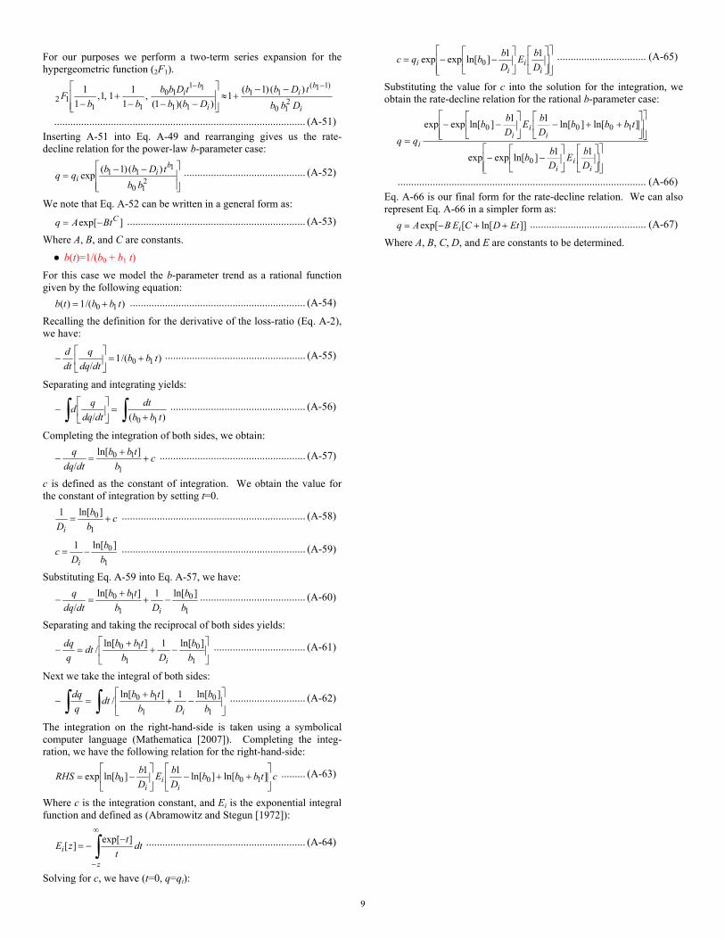
Figure 7 — Numerical Simulation Case 1: Production forecast (Log-Log) plot — Horizontal gas well with four transverse fractures (all models are shown).
Figure 8 — Numerical Simulation Case 2: History (Semi-Log) plot — Horizontal gas well.
16
Figure 9 — Numerical Simulation Case 2: "q-D-b" Log-Log plot — Horizontal gas well — definition of the "D- and b-" parameters, b-constant case (Arps' hyperbolic rate-decline relation).
Figure 10 — Numerical Simulation Case 2: "q-D-b" Log-Log plot — Horizontal gas well — definition of the "D- and b-" parameters, exponential b-parameter model.

17
Figure 11 — Numerical Simulation Case 2: "q-D-b" Log-Log plot — Horizontal gas well — definition of the "D- and b-" parameters, power-law b-parameter model.
Figure 12 — Numerical Simulation Case 2: "q-D-b" Log-Log plot — Horizontal gas well — definition of the "D- and b-" parameters, rational b-parameter model.

18
Figure 13 — Numerical Simulation Case 2: Production forecast (Semi-Log) plot — Horizontal gas well (all models are shown).
Figure 14 — Numerical Simulation Case 2: Production forecast (Log-Log) plot — Horizontal gas well (all models are shown).
19
Figure 15 — Field Example Case 1: History (Semi-Log) plot — Fractured well in a tight gas reservoir (ref. Ilk et al [2008c]).
Figure 16 — Field Example Case 1: "q-D-b" Log-Log plot — Fractured well in a tight gas reservoir (ref. Ilk et al [2008c]). ― definition of the "D and b" parameters, b-constant case (Arps' hyperbolic rate-decline relation).

20
Figure 17 — Field Example Case 1: "q-D-b" Log-Log plot — Fractured well in a tight gas reservoir (ref. Ilk et al [2008c]). ― definition of the "D and b" parameters, exponential b-parameter model.
Figure 18 — Field Example Case 1: "q-D-b" Log-Log plot — Fractured well in a tight gas reservoir (ref. Ilk et al [2008c]). ― definition of the "D and b" parameters, power-law b-parameter model.

21
Figure 19 — Field Example Case 1: "q-D-b" Log-Log plot — Fractured well in a tight gas reservoir (ref. Ilk et al [2008c]). ― definition of the "D and b" parameters, rational b-parameter model.
Figure 20 — Field Example Case 1: Production forecast (Semi-Log) plot — Fractured well in a tight gas reservoir (ref. Ilk et al [2008c]).
22
Figure 21 — Field Example Case 1: Production forecast (Log-Log) plot — Fractured well in a tight gas reservoir (ref. Ilk et al [2008c]).
Figure 22 — Field Example Case 2: History (Semi-Log) plot — Shale gas well (ref. Mattar et al [2008]).

23
Figure 23 — Field Example Case 2: "q-D-b" Log-Log plot — Shale gas well (ref. Mattar et al [2008]). ― definition of the "D and b" parameters, b-constant case (Arps' hyperbolic rate-decline relation).
Figure 24 — Field Example Case 2: "q-D-b" Log-Log plot — Shale gas well (ref. Mattar et al [2008]). ― definition of the "D and b" parameters, exponential b-parameter model.

24
Figure 25 — Field Example Case 2: "q-D-b" Log-Log plot — Shale gas well (ref. Mattar et al [2008]). ― definition of the "D and b" parameters, power-law b-parameter model.
Figure 26 — Field Example Case 2: "q-D-b" Log-Log plot — Shale gas well (ref. Mattar et al [2008]). ― definition of the "D and b" parameters, rational b-parameter model.
25
Figure 27 — Field Example Case 2: Production forecast (Semi-Log) plot — Shale gas well (ref. Mattar et al [2008]).
Figure 28 — Field Example Case 2: Production forecast (Log-Log) plot — Shale gas well (ref. Mattar et al [2008]).

2009 Canadian International Petroluem Conference — Calgary, AB (Canada) — 16–18 June 2009 A New Series of Rate Decline Relations Based on the Diagnosis of Rate-Time Data
(Boulis/Ilk/Blasingame)A.S.Boulis— Texas A&M University (16 June 2009) Sl
ide
—1/
35
A.S. Boulis,* Texas A&M U.D. Ilk, Texas A&M U.
and T.A. Blasingame, Texas A&M U.*Department of Petroleum Engineering
Texas A&M UniversityCollege Station, TX 77843-3116
+1.979.845.2292 — [email protected]
CIPC 2009-202A New Series of
Rate Decline Relations Based on the Diagnosis of Rate-Time Data

2009 Canadian International Petroluem Conference — Calgary, AB (Canada) — 16–18 June 2009 A New Series of Rate Decline Relations Based on the Diagnosis of Rate-Time Data
(Boulis/Ilk/Blasingame)A.S.Boulis— Texas A&M University (16 June 2009) Sl
ide
—2/
35
Presentation Outline●Overview●Rationale■ b-parameter as a function of time■ b(t) is to be defined by rate-time data.
●Development of the New Rate Decline Models:■ b(t) = constant (Arps' hyperbolic rate decline)■ b(t) = b0 Exp[-b1t] (exponential function)■ b(t) = b0t -b1 (power law function)■ b(t) = 1/(b0 + b1t) (rational function)
●Application of the New Rate Decline Models:■ Synthetic Cases
— Horizontal Gas Well with Multiple Transverse Fractures (SPE 119897 Data)
— Horizontal Gas Well ■ Field Cases
— Fractured Tight Gas Well (Bossier Tight Gas Sand Field)— Shale Gas (Barnett Shale)
●Conclusions and Recommendations
(Out
line)
●

2009 Canadian International Petroluem Conference — Calgary, AB (Canada) — 16–18 June 2009 A New Series of Rate Decline Relations Based on the Diagnosis of Rate-Time Data
(Boulis/Ilk/Blasingame)A.S.Boulis— Texas A&M University (16 June 2009) Sl
ide
—3/
35
Rationale:●Definitions:■ D-parameter: Ratio of rate to rate derivative (i.e., "loss ratio").
■ b-parameter: Derivative of the "loss ratio".
⎥⎦⎤
⎢⎣⎡≡
⎥⎦
⎤⎢⎣
⎡−≡⎥⎦
⎤⎢⎣⎡≡
DdQdqb
dtdqq
dtd
Ddtdb
1or
/1
⎥⎦
⎤⎢⎣
⎡−≡−≡
dQdqD
dtdqq
Dor
/1 (R
atio
nale
) ●○

2009 Canadian International Petroluem Conference — Calgary, AB (Canada) — 16–18 June 2009 A New Series of Rate Decline Relations Based on the Diagnosis of Rate-Time Data
(Boulis/Ilk/Blasingame)A.S.Boulis— Texas A&M University (16 June 2009) Sl
ide
—4/
35
Rationale:●Objectives:■ b-parameter is NEVER CONSTANT — changes continuously
with time.■ PROVIDE a unique, diagnostic understanding of the
b-parameter.■ PROPOSE new rate decline relations based on the character of
the b-parameter.■ PROVIDE examples for each b-parameter rate decline model.
"q-D-b Plot" (Diagnostic plot for the character of the b-parameter).
(Rat
iona
le) ●
●
[From: Mattar, L., Gault, B., Morad, K., Clarkson, C., Freeman, C.M., Ilk, D., Blasingame, T.A.: "Production Analysis and Forecasting of Shale Gas Reservoirs: Case History-based Approach," paper SPE 119897 presented at the 2008 Shale Gas Production Conference, Irving, TX, 16-17 November 2008. ]
2009 Canadian International Petroluem Conference — Calgary, AB (Canada) — 16–18 June 2009 A New Series of Rate Decline Relations Based on the Diagnosis of Rate-Time Data
(Boulis/Ilk/Blasingame)A.S.Boulis— Texas A&M University (16 June 2009) Sl
ide
—5/
35
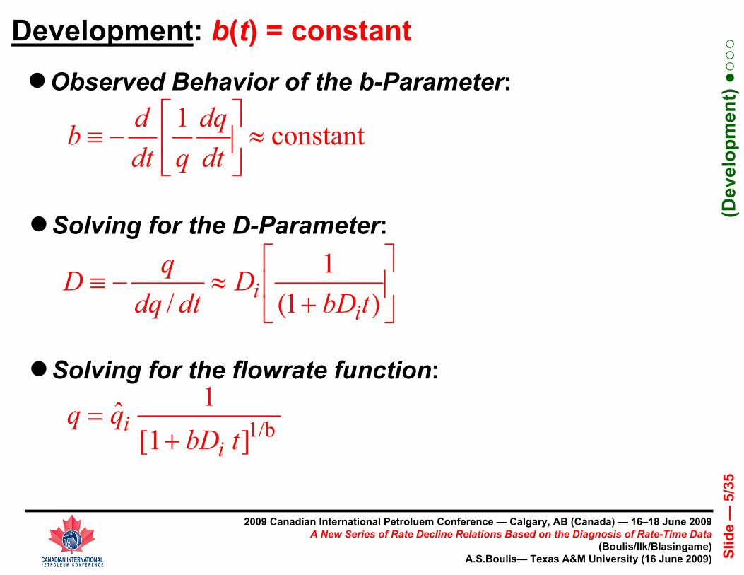
Development: b(t) = constant
constant1≈⎥
⎦
⎤⎢⎣
⎡−≡
dtdq
qdtdb
●Observed Behavior of the b-Parameter:
●Solving for the D-Parameter:
1/b] [11 ˆ
tbDqq
ii
+=
●Solving for the flowrate function:
⎥⎦
⎤⎢⎣
⎡
+≈−≡
)1(1
/ tbDD
dtdqqD
ii
(Dev
elop
men
t) ●○
○○
2009 Canadian International Petroluem Conference — Calgary, AB (Canada) — 16–18 June 2009 A New Series of Rate Decline Relations Based on the Diagnosis of Rate-Time Data
(Boulis/Ilk/Blasingame)A.S.Boulis— Texas A&M University (16 June 2009) Sl
ide
—6/
35
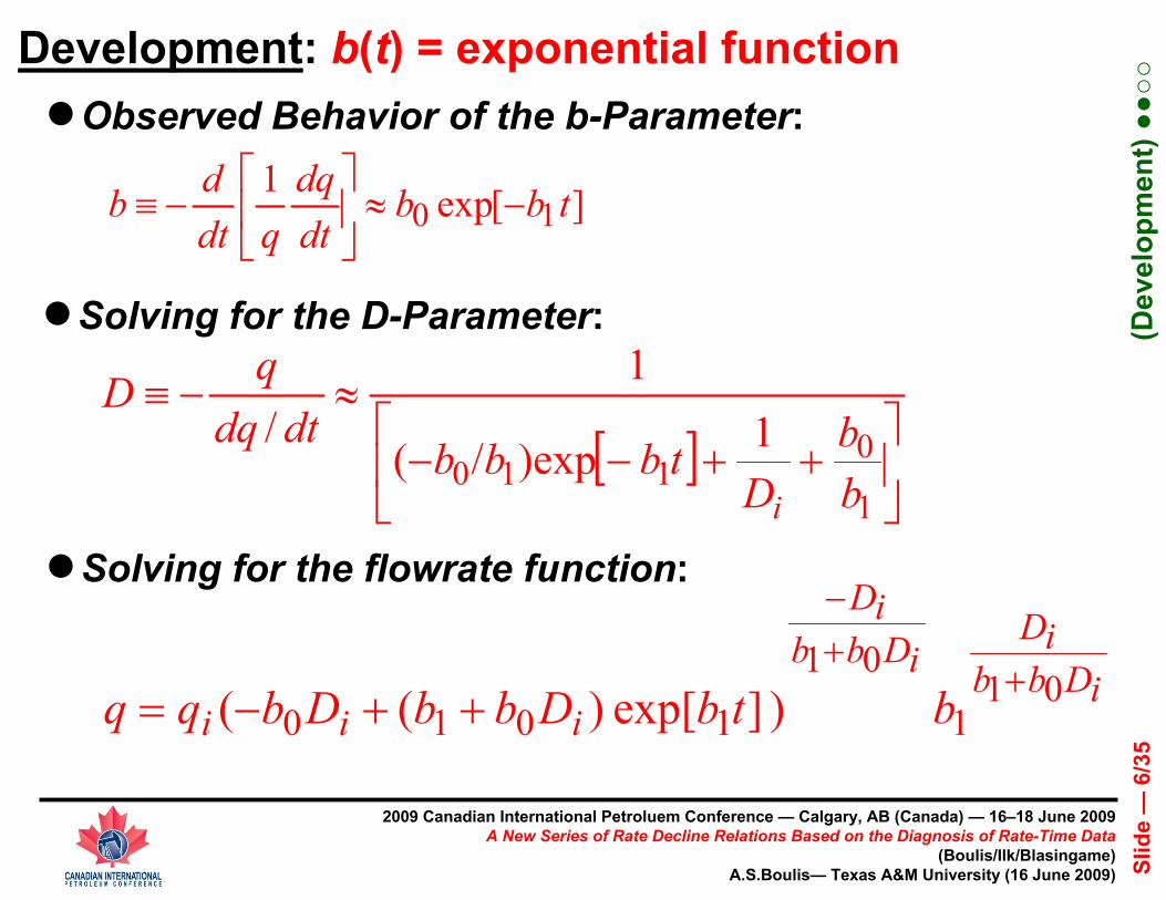
Development: b(t) = exponential function●Observed Behavior of the b-Parameter:
●Solving for the D-Parameter:
[ ] ⎥⎦
⎤⎢⎣
⎡++−−
≈−≡
1
0110
1)exp/(
1/
bb
Dtbbb
dtdqqD
i
●Solving for the flowrate function:
iDbbiD
iDbbiD
iii btbDbbDbqq 011
01
1010 ) ]exp[ )((+
+−
++−=
][exp110 tbb
dtdq
qdtdb −≈⎥
⎦
⎤⎢⎣
⎡−≡
(Dev
elop
men
t) ●●
○○
2009 Canadian International Petroluem Conference — Calgary, AB (Canada) — 16–18 June 2009 A New Series of Rate Decline Relations Based on the Diagnosis of Rate-Time Data
(Boulis/Ilk/Blasingame)A.S.Boulis— Texas A&M University (16 June 2009) Sl
ide
—7/
35
Development: b(t) = power law function
101 btb
dtdq
qdtdb −=⎥
⎦
⎤⎢⎣
⎡−≡
●Observed Behavior of the b-Parameter:
●Solving for the D-Parameter:
⎥⎥⎦
⎤
⎢⎢⎣
⎡ −+= 2
10
111
)( )(-1
exp ˆbb
tDbbqq
bi
i
●Solving for the flowrate function:11
10 111
1/ 1
bDbtbdtdq
qD
i
b+−
−−
≈−≡ −
(Dev
elop
men
t) ●●
●○
2009 Canadian International Petroluem Conference — Calgary, AB (Canada) — 16–18 June 2009 A New Series of Rate Decline Relations Based on the Diagnosis of Rate-Time Data
(Boulis/Ilk/Blasingame)A.S.Boulis— Texas A&M University (16 June 2009) Sl
ide
—8/
35
Development: b(t) = rational function●Observed Behavior of the b-Parameter:
●Solving for the D-Parameter:
1
10
1
0 )(ln)(ln11
/b
tbbbb
Ddtdq
qD
i
+−+−
≈−≡
●Solving for the flowrate function:[ ][ ][ ][ ] )ln( exp
)ln( exp
01
101bBEA
tbbBEAqq i +++
=
tbbdtdq
qdtdb
10
11+
≈⎥⎦
⎤⎢⎣
⎡−≡
Where: and ⎥⎥⎦
⎤
⎢⎢⎣
⎡⎥⎦
⎤⎢⎣
⎡+−−−=
iDbbbA 1lnexp1
01 ⎥
⎦
⎤⎢⎣
⎡+−=
iDbbbB 1)ln(
1
01
(Dev
elop
men
t) ●●
●●

2009 Canadian International Petroluem Conference — Calgary, AB (Canada) — 16–18 June 2009 A New Series of Rate Decline Relations Based on the Diagnosis of Rate-Time Data
(Boulis/Ilk/Blasingame)A.S.Boulis— Texas A&M University (16 June 2009) Sl
ide
—9/
35
Rate Decline Models: Horizontal Fractured Gas Well
a. Plotting Function 1: (Horizontal Fractured Gas Well), q-D-b vs t, Plot b(t)=constant model.
b. Plotting Function 2: (Horizontal Fractured Gas Well), q-D-b vs t, Plot b(t)=exponential model.
c. Plotting Function 3: (Horizontal Fractured Gas Well), q-D-b vs t, Plot b(t)=power-law model.
d. Plotting Function 4: (Horizontal Fractured Gas Well), q-D-b vs t, Plot b(t)=rational model.
(Num
eric
al S
imul
atio
n C
ase
1) ●○○
○○

2009 Canadian International Petroluem Conference — Calgary, AB (Canada) — 16–18 June 2009 A New Series of Rate Decline Relations Based on the Diagnosis of Rate-Time Data
(Boulis/Ilk/Blasingame)A.S.Boulis— Texas A&M University (16 June 2009) Sl
ide
—10
/35
●Discussion: ■Simulation Case 1 — Horizontal Gas Well with multiple
transverse fractures.■D- and b-parameters are computed using the rate-time data.■This model is ONLY applicable for the boundary-dominated flow.■b = constant model always yields highest estimates of reserves.
Rate Decline Models: b(t) = constant
(Num
eric
al S
imul
atio
n C
ase
1) ●●○
○○

2009 Canadian International Petroluem Conference — Calgary, AB (Canada) — 16–18 June 2009 A New Series of Rate Decline Relations Based on the Diagnosis of Rate-Time Data
(Boulis/Ilk/Blasingame)A.S.Boulis— Texas A&M University (16 June 2009) Sl
ide
—11
/35
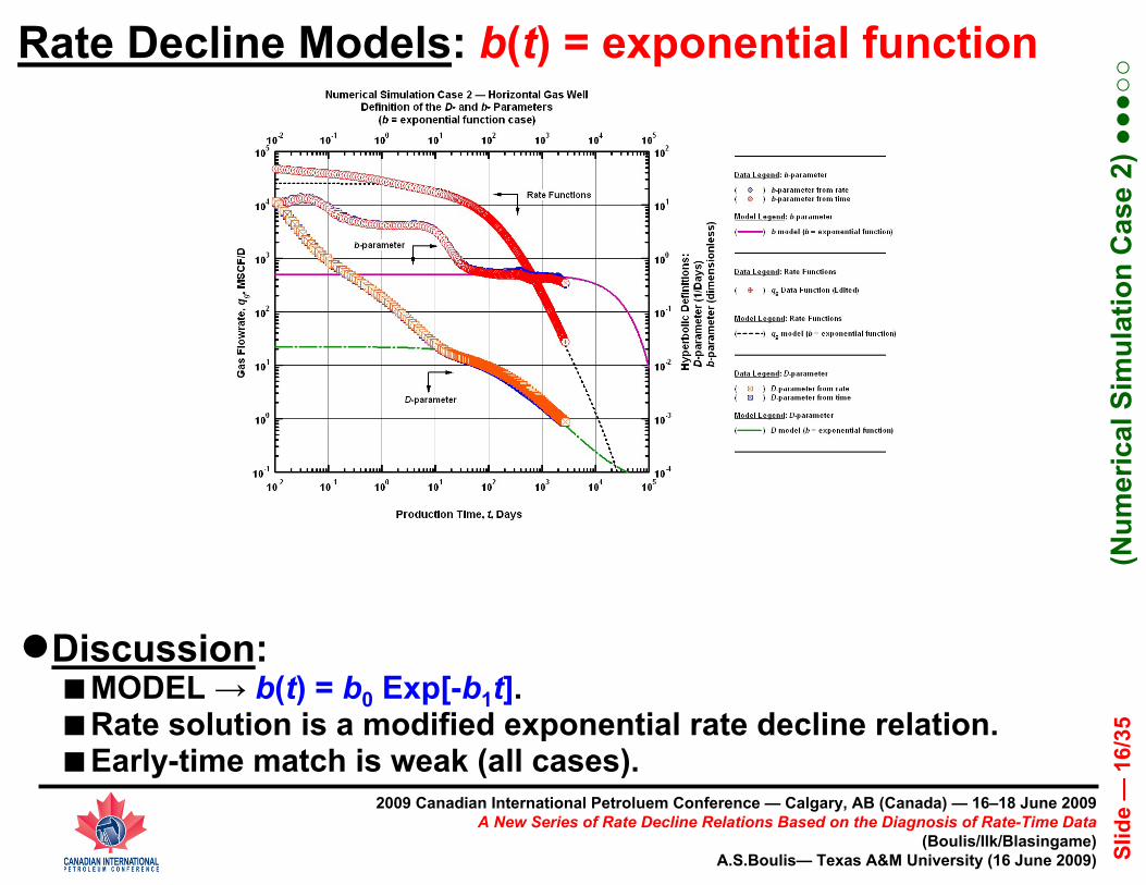
●Discussion: ■MODEL → b(t) = b0 Exp[-b1t]. ■Rate solution is a modified exponential rate decline relation.■More conservative than the b = constant case.■Early-time match is weak (all cases).
Rate Decline Models: b(t) = exponential function
(Num
eric
al S
imul
atio
n C
ase
1) ●●●
○○
2009 Canadian International Petroluem Conference — Calgary, AB (Canada) — 16–18 June 2009 A New Series of Rate Decline Relations Based on the Diagnosis of Rate-Time Data
(Boulis/Ilk/Blasingame)A.S.Boulis— Texas A&M University (16 June 2009) Sl
ide
—12
/35
●Discussion: ■MODEL → b(t) = b0 t -b1.■Rate solution contains a Hypergeometric function.■May be applicable for all flow regimes.■Very good matches with the data for all the flow regimes.
Rate Decline Models: b(t) = power-law function
(Num
eric
al S
imul
atio
n C
ase
1) ●●●
●○

2009 Canadian International Petroluem Conference — Calgary, AB (Canada) — 16–18 June 2009 A New Series of Rate Decline Relations Based on the Diagnosis of Rate-Time Data
(Boulis/Ilk/Blasingame)A.S.Boulis— Texas A&M University (16 June 2009) Sl
ide
—13
/35
●Discussion: ■MODEL → b(t) = 1/(b0 + b1t).■Rate solution includes "Exponential Integral" term.■May be applicable for all flow regimes.■Satisfactory matches with the computed data for all the flow
regimes.
Rate Decline Models: b(t) = rational function
(Num
eric
al S
imul
atio
n C
ase
1) ●●●
●●

2009 Canadian International Petroluem Conference — Calgary, AB (Canada) — 16–18 June 2009 A New Series of Rate Decline Relations Based on the Diagnosis of Rate-Time Data
(Boulis/Ilk/Blasingame)A.S.Boulis— Texas A&M University (16 June 2009) Sl
ide
—14
/35
a. Plotting Function 1: (Horizontal Gas Well), q-D-b vs t, Plot b(t)=constant model.
b. Plotting Function 2: (Horizontal Gas Well), q-D-b vs t,Plot b(t)=exponential model.
c. Plotting Function 3: (Horizontal Gas Well), q-D-b vs t, Plot b(t)=power-law model.
d. Plotting Function 4: (Horizontal Gas Well), q-D-b vs t, Plot b(t)=rational model.
Rate Decline Models: Horizontal Gas Well
(Num
eric
al S
imul
atio
n C
ase
2) ●○○
○○
2009 Canadian International Petroluem Conference — Calgary, AB (Canada) — 16–18 June 2009 A New Series of Rate Decline Relations Based on the Diagnosis of Rate-Time Data
(Boulis/Ilk/Blasingame)A.S.Boulis— Texas A&M University (16 June 2009) Sl
ide
—15
/35
●Discussion: ■Simulation Case 2 — Horizontal Gas Well.■D- and b-parameters are computed using the rate-time data.■This model is ONLY applicable for the boundary-dominated flow.■ In this case the model estimated the exact amount of reserves.
Rate Decline Models: b(t) = constant
(Num
eric
al S
imul
atio
n C
ase
2) ●●○
○○
2009 Canadian International Petroluem Conference — Calgary, AB (Canada) — 16–18 June 2009 A New Series of Rate Decline Relations Based on the Diagnosis of Rate-Time Data
(Boulis/Ilk/Blasingame)A.S.Boulis— Texas A&M University (16 June 2009) Sl
ide
—16
/35
●Discussion: ■MODEL → b(t) = b0 Exp[-b1t]. ■Rate solution is a modified exponential rate decline relation.■Early-time match is weak (all cases).
Rate Decline Models: b(t) = exponential function
(Num
eric
al S
imul
atio
n C
ase
2) ●●●
○○
2009 Canadian International Petroluem Conference — Calgary, AB (Canada) — 16–18 June 2009 A New Series of Rate Decline Relations Based on the Diagnosis of Rate-Time Data
(Boulis/Ilk/Blasingame)A.S.Boulis— Texas A&M University (16 June 2009) Sl
ide
—17
/35
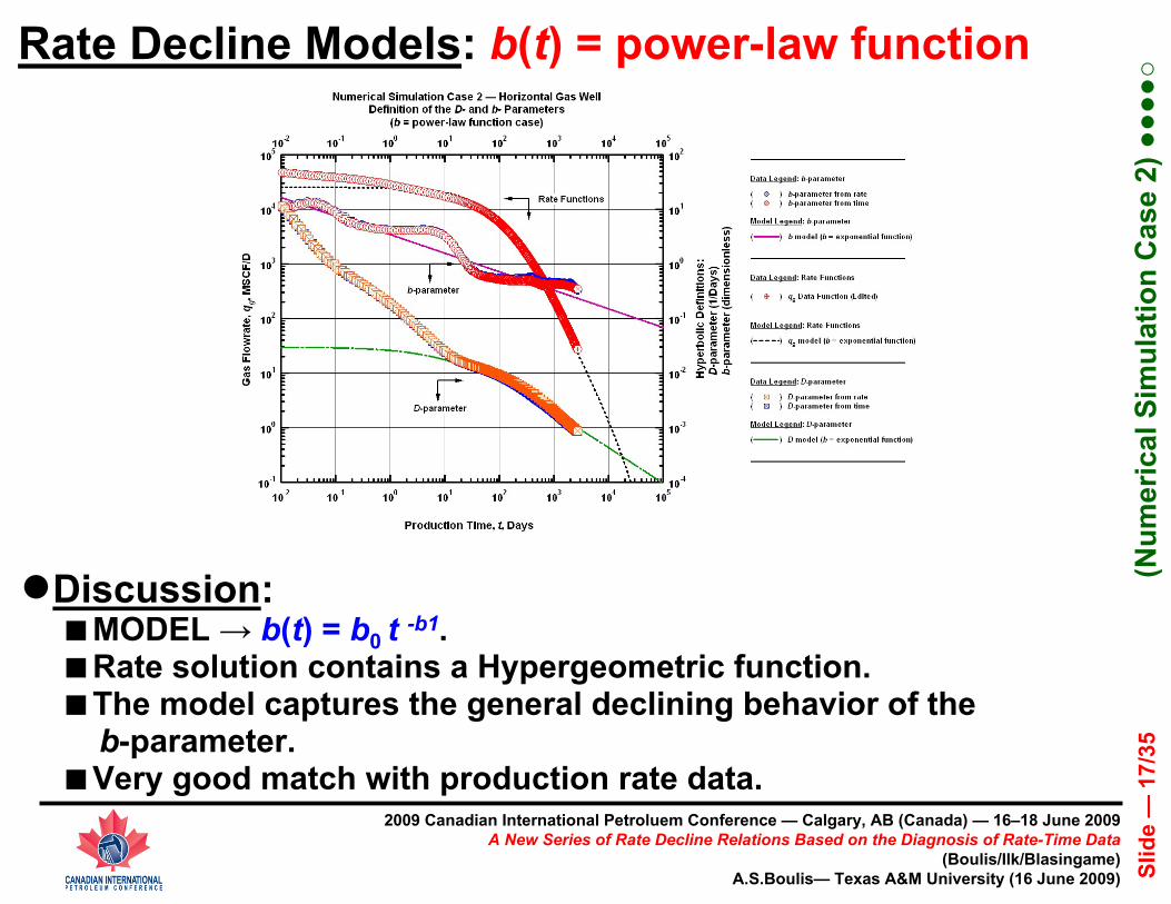
●Discussion: ■MODEL → b(t) = b0 t -b1. ■Rate solution contains a Hypergeometric function.■The model captures the general declining behavior of the
b-parameter.■Very good match with production rate data.
Rate Decline Models: b(t) = power-law function
(Num
eric
al S
imul
atio
n C
ase
2) ●●●
●○
2009 Canadian International Petroluem Conference — Calgary, AB (Canada) — 16–18 June 2009 A New Series of Rate Decline Relations Based on the Diagnosis of Rate-Time Data
(Boulis/Ilk/Blasingame)A.S.Boulis— Texas A&M University (16 June 2009) Sl
ide
—18
/35
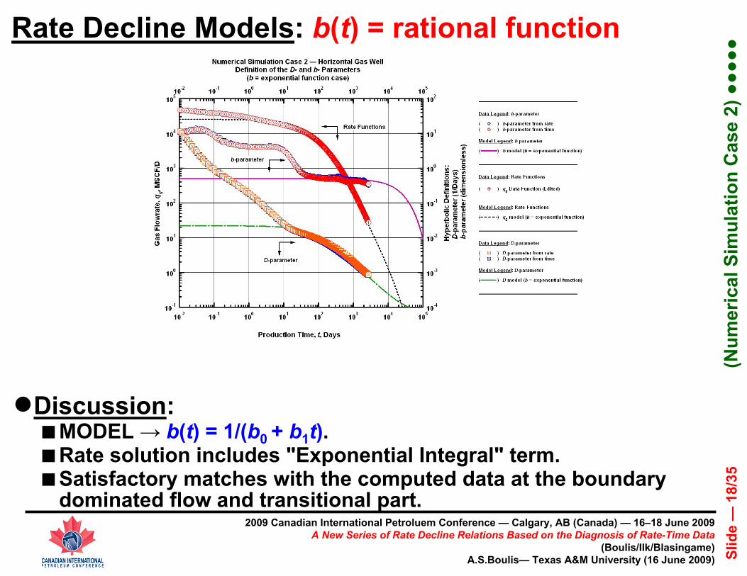
●Discussion: ■MODEL → b(t) = 1/(b0 + b1t).■Rate solution includes "Exponential Integral" term.■Satisfactory matches with the computed data at the boundary
dominated flow and transitional part.
Rate Decline Models: b(t) = rational function
(Num
eric
al S
imul
atio
n C
ase
2) ●●●
●●
2009 Canadian International Petroluem Conference — Calgary, AB (Canada) — 16–18 June 2009 A New Series of Rate Decline Relations Based on the Diagnosis of Rate-Time Data
(Boulis/Ilk/Blasingame)A.S.Boulis— Texas A&M University (16 June 2009) Sl
ide
—19
/35
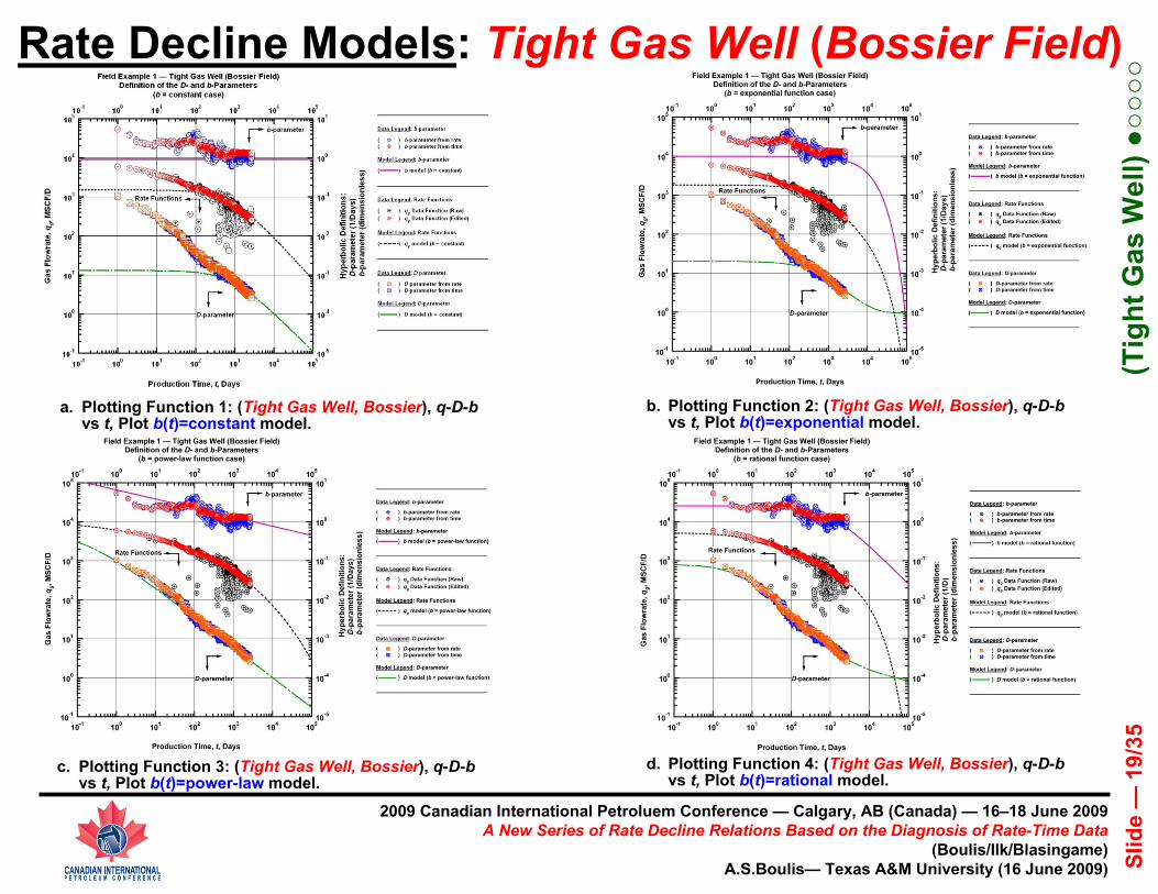
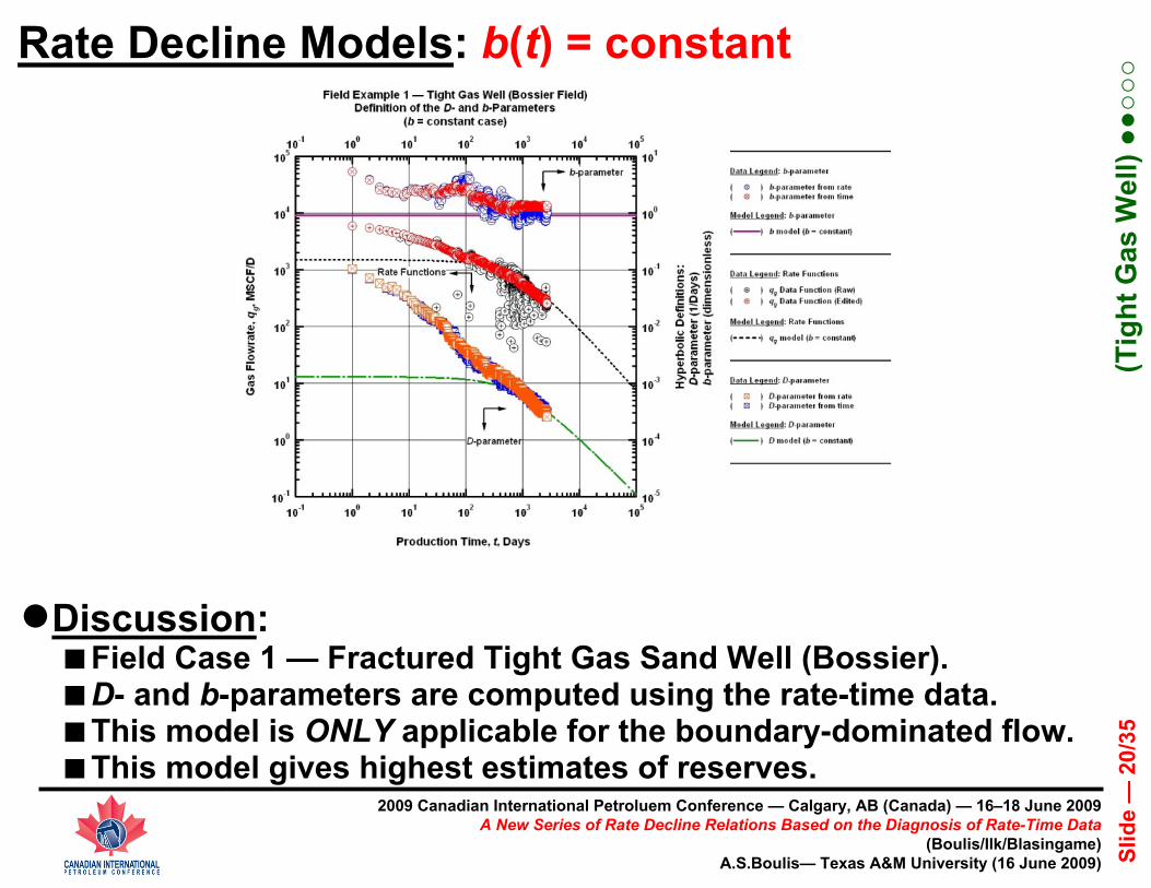
a. Plotting Function 1: (Tight Gas Well, Bossier), q-D-bvs t, Plot b(t)=constant model.
b. Plotting Function 2: (Tight Gas Well, Bossier), q-D-bvs t, Plot b(t)=exponential model.
c. Plotting Function 3: (Tight Gas Well, Bossier), q-D-bvs t, Plot b(t)=power-law model.
d. Plotting Function 4: (Tight Gas Well, Bossier), q-D-bvs t, Plot b(t)=rational model.
Rate Decline Models: Tight Gas Well (Bossier Field)
(Tig
ht G
as W
ell) ●○
○○○
2009 Canadian International Petroluem Conference — Calgary, AB (Canada) — 16–18 June 2009 A New Series of Rate Decline Relations Based on the Diagnosis of Rate-Time Data
(Boulis/Ilk/Blasingame)A.S.Boulis— Texas A&M University (16 June 2009) Sl
ide
—20
/35
●Discussion: ■Field Case 1 — Fractured Tight Gas Sand Well (Bossier).■D- and b-parameters are computed using the rate-time data.■This model is ONLY applicable for the boundary-dominated flow.■This model gives highest estimates of reserves.
Rate Decline Models: b(t) = constant
(Tig
ht G
as W
ell) ●●
○○○

2009 Canadian International Petroluem Conference — Calgary, AB (Canada) — 16–18 June 2009 A New Series of Rate Decline Relations Based on the Diagnosis of Rate-Time Data
(Boulis/Ilk/Blasingame)A.S.Boulis— Texas A&M University (16 June 2009) Sl
ide
—21
/35
●Discussion: ■MODEL → b(t) = b0 Exp[-b1t]. ■Rate solution is a modified exponential rate decline relation.■Satisfactory matches at the boundary dominated flow regime.■Early-time match is weak (all cases).
Rate Decline Models: b(t) = exponential function
(Tig
ht G
as W
ell) ●●
●○○

2009 Canadian International Petroluem Conference — Calgary, AB (Canada) — 16–18 June 2009 A New Series of Rate Decline Relations Based on the Diagnosis of Rate-Time Data
(Boulis/Ilk/Blasingame)A.S.Boulis— Texas A&M University (16 June 2009) Sl
ide
—22
/35
●Discussion: ■MODEL → b(t) = b0 t -b1. ■Rate solution contains a Hypergeometric function.■Very good matches with the data for all the flow regimes.
Rate Decline Models: b(t) = power-law function
(Tig
ht G
as W
ell) ●●
●●○
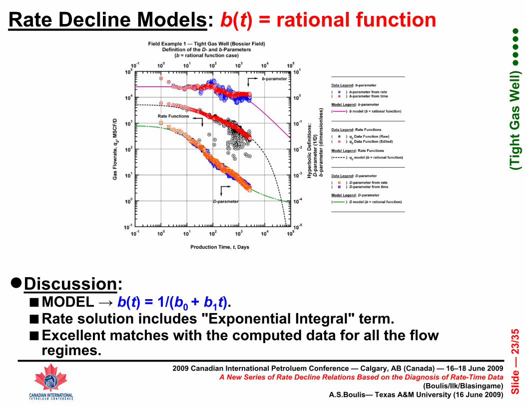
2009 Canadian International Petroluem Conference — Calgary, AB (Canada) — 16–18 June 2009 A New Series of Rate Decline Relations Based on the Diagnosis of Rate-Time Data
(Boulis/Ilk/Blasingame)A.S.Boulis— Texas A&M University (16 June 2009) Sl
ide
—23
/35
●Discussion: ■MODEL → b(t) = 1/(b0 + b1t).■Rate solution includes "Exponential Integral" term.■Excellent matches with the computed data for all the flow
regimes.
Rate Decline Models: b(t) = rational function
(Tig
ht G
as W
ell) ●●
●●●

2009 Canadian International Petroluem Conference — Calgary, AB (Canada) — 16–18 June 2009 A New Series of Rate Decline Relations Based on the Diagnosis of Rate-Time Data
(Boulis/Ilk/Blasingame)A.S.Boulis— Texas A&M University (16 June 2009) Sl
ide
—24
/35
a. Plotting Function 1: (Shale Gas Well, Barnett), q-D-bvs t, Plot b(t)=constant model.
b. Plotting Function 2: (Shale Gas Well, Barnett), q-D-bvs t, Plot b(t)=exponential model.
c. Plotting Function 3: (Shale Gas Well, Barnett), q-D-bvs t, Plot b(t)=power-law model.
d. Plotting Function 4: (Shale Gas Well, Barnett), q-D-bvs t, Plot b(t)=rational model.
Rate Decline Models: Shale Gas Well (Barnett)
(Sha
le G
as W
ell) ●○
○○○

2009 Canadian International Petroluem Conference — Calgary, AB (Canada) — 16–18 June 2009 A New Series of Rate Decline Relations Based on the Diagnosis of Rate-Time Data
(Boulis/Ilk/Blasingame)A.S.Boulis— Texas A&M University (16 June 2009) Sl
ide
—25
/35
●Discussion: ■Field Case 2 — Shale Gas Well (Barnett).■D- and b-parameters are computed using the rate-time data.■This model is ONLY applicable for the boundary-dominated flow.■This model gives highest estimates of reserves.
Rate Decline Models: b(t) = constant
(Sha
le G
as W
ell) ●●
○○○
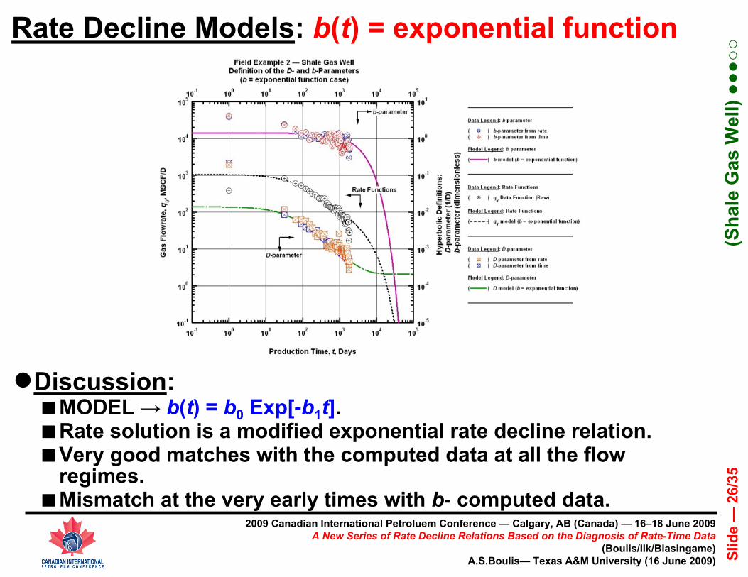
2009 Canadian International Petroluem Conference — Calgary, AB (Canada) — 16–18 June 2009 A New Series of Rate Decline Relations Based on the Diagnosis of Rate-Time Data
(Boulis/Ilk/Blasingame)A.S.Boulis— Texas A&M University (16 June 2009) Sl
ide
—26
/35
●Discussion: ■MODEL → b(t) = b0 Exp[-b1t]. ■Rate solution is a modified exponential rate decline relation.■Very good matches with the computed data at all the flow
regimes.■Mismatch at the very early times with b- computed data.
Rate Decline Models: b(t) = exponential function
(Sha
le G
as W
ell) ●●
●○○
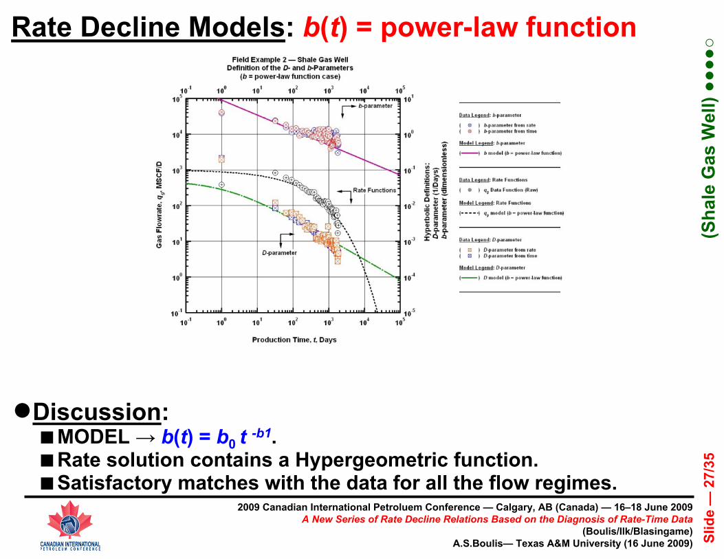
2009 Canadian International Petroluem Conference — Calgary, AB (Canada) — 16–18 June 2009 A New Series of Rate Decline Relations Based on the Diagnosis of Rate-Time Data
(Boulis/Ilk/Blasingame)A.S.Boulis— Texas A&M University (16 June 2009) Sl
ide
—27
/35
●Discussion: ■MODEL → b(t) = b0 t -b1.■Rate solution contains a Hypergeometric function.■Satisfactory matches with the data for all the flow regimes.
Rate Decline Models: b(t) = power-law function
(Sha
le G
as W
ell) ●●
●●○
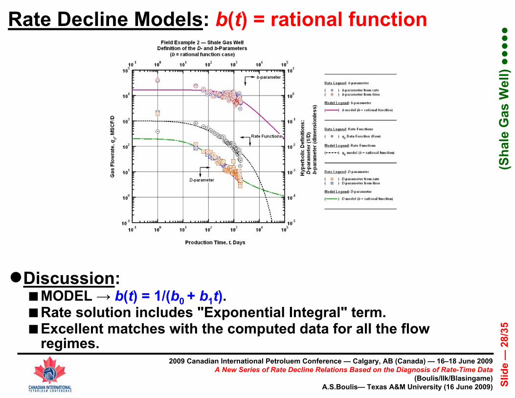
2009 Canadian International Petroluem Conference — Calgary, AB (Canada) — 16–18 June 2009 A New Series of Rate Decline Relations Based on the Diagnosis of Rate-Time Data
(Boulis/Ilk/Blasingame)A.S.Boulis— Texas A&M University (16 June 2009) Sl
ide
—28
/35
●Discussion: ■MODEL → b(t) = 1/(b0 + b1t).■Rate solution includes "Exponential Integral" term.■Excellent matches with the computed data for all the flow
regimes.
Rate Decline Models: b(t) = rational function
(Sha
le G
as W
ell) ●●
●●●
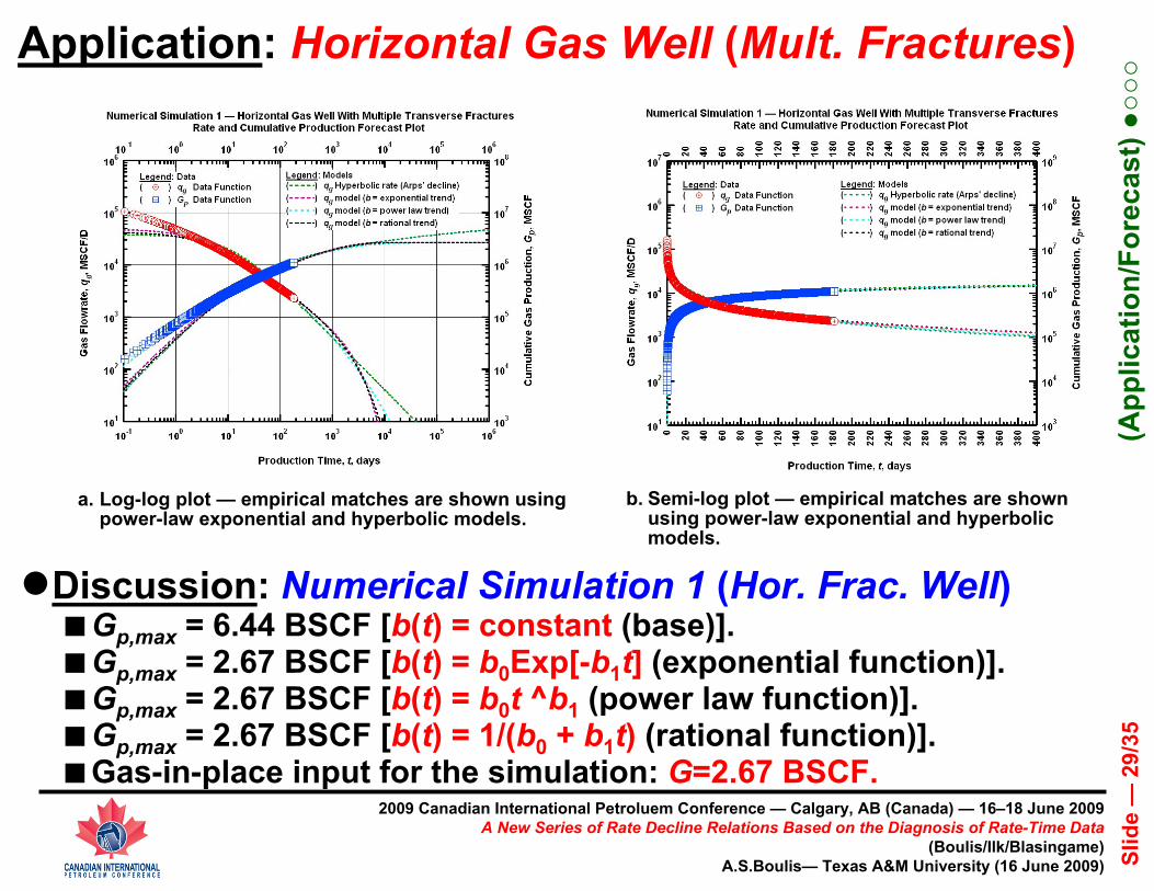
2009 Canadian International Petroluem Conference — Calgary, AB (Canada) — 16–18 June 2009 A New Series of Rate Decline Relations Based on the Diagnosis of Rate-Time Data
(Boulis/Ilk/Blasingame)A.S.Boulis— Texas A&M University (16 June 2009) Sl
ide
—29
/35
●Discussion: Numerical Simulation 1 (Hor. Frac. Well)■Gp,max = 6.44 BSCF [b(t) = constant (base)].■Gp,max = 2.67 BSCF [b(t) = b0Exp[-b1t] (exponential function)].■Gp,max = 2.67 BSCF [b(t) = b0t ^b1 (power law function)].■Gp,max = 2.67 BSCF [b(t) = 1/(b0 + b1t) (rational function)].■Gas-in-place input for the simulation: G=2.67 BSCF.
a. Log-log plot — empirical matches are shown using power-law exponential and hyperbolic models.
b. Semi-log plot — empirical matches are shown using power-law exponential and hyperbolic models.
Application: Horizontal Gas Well (Mult. Fractures)
(App
licat
ion/
Fore
cast
) ●○○
○
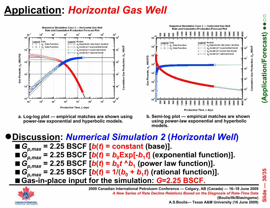
2009 Canadian International Petroluem Conference — Calgary, AB (Canada) — 16–18 June 2009 A New Series of Rate Decline Relations Based on the Diagnosis of Rate-Time Data
(Boulis/Ilk/Blasingame)A.S.Boulis— Texas A&M University (16 June 2009) Sl
ide
—30
/35
●Discussion: Numerical Simulation 2 (Horizontal Well)■Gp,max = 2.25 BSCF [b(t) = constant (base)].■Gp,max = 2.25 BSCF [b(t) = b0Exp[-b1t] (exponential function)].■Gp,max = 2.25 BSCF [b(t) = b0t ^b1 (power law function)].■Gp,max = 2.25 BSCF [b(t) = 1/(b0 + b1t) (rational function)].■Gas-in-place input for the simulation: G=2.25 BSCF.
a. Log-log plot — empirical matches are shown using power-law exponential and hyperbolic models.
b. Semi-log plot — empirical matches are shown using power-law exponential and hyperbolic models.
Application: Horizontal Gas Well
(App
licat
ion/
Fore
cast
) ●●○
○

2009 Canadian International Petroluem Conference — Calgary, AB (Canada) — 16–18 June 2009 A New Series of Rate Decline Relations Based on the Diagnosis of Rate-Time Data
(Boulis/Ilk/Blasingame)A.S.Boulis— Texas A&M University (16 June 2009) Sl
ide
—31
/35
●Discussion: Field Case 1 (Fractured Tight Gas Well)■Gp,max = 8.40 BSCF [b(t) = constant (base)].■Gp,max = 3.00 BSCF [b(t) = b0Exp[-b1t] (exponential function)].■Gp,max = 3.00 BSCF [b(t) = b0t ^b1 (power law function)].■Gp,max = 3.00 BSCF [b(t) = 1/(b0 + b1t) (rational function)].■Model-based analysis yields G=3.00 BSCF.
a. Log-log plot — empirical matches are shown using power-law exponential and hyperbolic models.
b. Semi-log plot — empirical matches are shown using power-law exponential and hyperbolic models.
Application: Tight Gas Well (Bossier Field)
(App
licat
ion/
Fore
cast
) ●●●
○
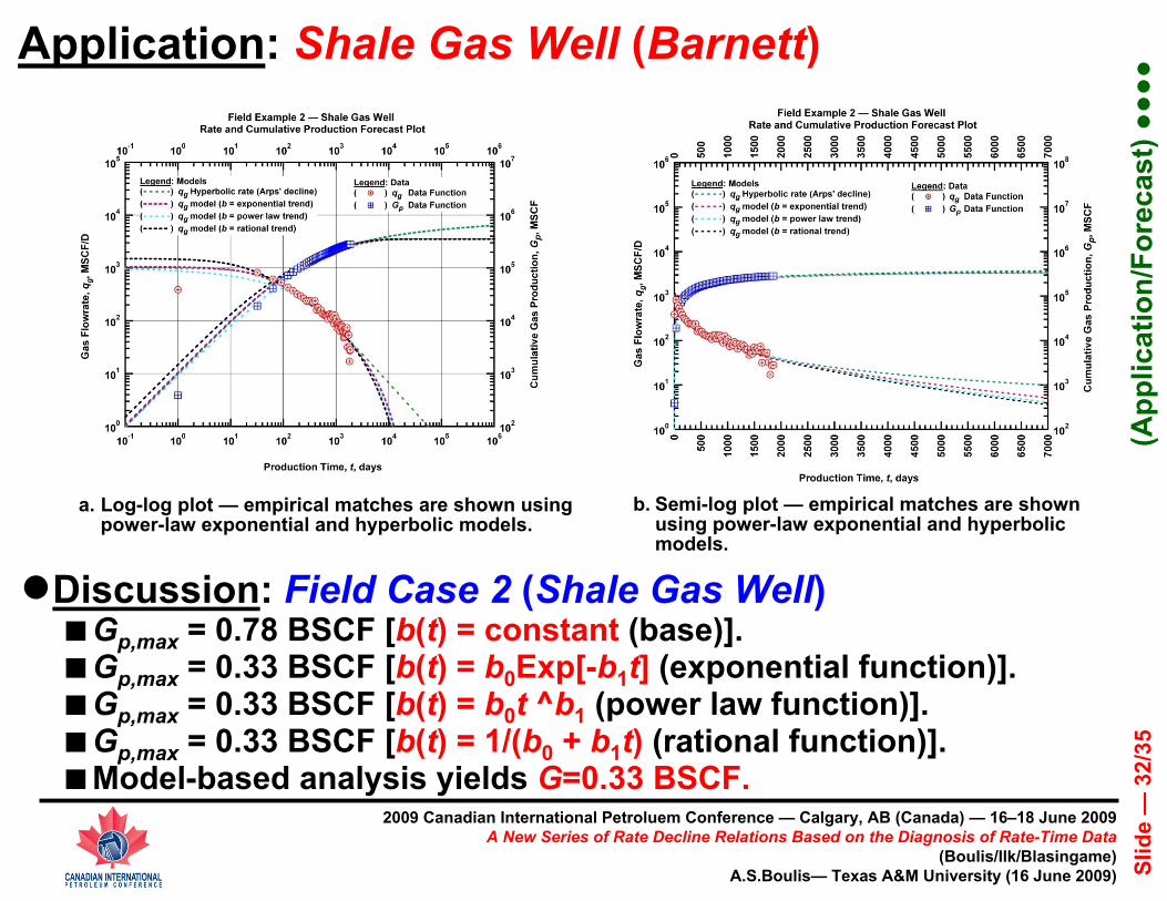
2009 Canadian International Petroluem Conference — Calgary, AB (Canada) — 16–18 June 2009 A New Series of Rate Decline Relations Based on the Diagnosis of Rate-Time Data
(Boulis/Ilk/Blasingame)A.S.Boulis— Texas A&M University (16 June 2009) Sl
ide
—32
/35
●Discussion: Field Case 2 (Shale Gas Well)■Gp,max = 0.78 BSCF [b(t) = constant (base)].■Gp,max = 0.33 BSCF [b(t) = b0Exp[-b1t] (exponential function)].■Gp,max = 0.33 BSCF [b(t) = b0t ^b1 (power law function)].■Gp,max = 0.33 BSCF [b(t) = 1/(b0 + b1t) (rational function)].■Model-based analysis yields G=0.33 BSCF.
a. Log-log plot — empirical matches are shown using power-law exponential and hyperbolic models.
b. Semi-log plot — empirical matches are shown using power-law exponential and hyperbolic models.
Application: Shale Gas Well (Barnett)
(App
licat
ion/
Fore
cast
) ●●●
●

2009 Canadian International Petroluem Conference — Calgary, AB (Canada) — 16–18 June 2009 A New Series of Rate Decline Relations Based on the Diagnosis of Rate-Time Data
(Boulis/Ilk/Blasingame)A.S.Boulis— Texas A&M University (16 June 2009) Sl
ide
—33
/35
● The decline b-parameter is NOT constant, but it can best be described as a decreasing function with time.
● The Arps' Hyperbolic Rate Decline Relation usually over-estimates the reserve extrapolations.
● The newly proposed b-parameter models have yielded improved matches with the data for all the flow regimes and more accurate/constrained reserve estimates (b-rational — excellent matches and forecasts for all the investigated cases.
Conclusions:
(Con
clus
ions
) ●

2009 Canadian International Petroluem Conference — Calgary, AB (Canada) — 16–18 June 2009 A New Series of Rate Decline Relations Based on the Diagnosis of Rate-Time Data
(Boulis/Ilk/Blasingame)A.S.Boulis— Texas A&M University (16 June 2009) Sl
ide
—34
/35
● The behavior of the b-parameter (with time) must be investigated further — new models should be developed.
● Extend the application of the existing models to more complex well/reservoir cases.
● Further validation of the models with the analytical solutions — Numerical Simulation Cases.
Recommendations:
(Rec
omm
enda
tions
) ●

2009 Canadian International Petroluem Conference — Calgary, AB (Canada) — 16–18 June 2009 A New Series of Rate Decline Relations Based on the Diagnosis of Rate-Time Data
(Boulis/Ilk/Blasingame)A.S.Boulis— Texas A&M University (16 June 2009) Sl
ide
—35
/35
A.S. Boulis,* Texas A&M U.D. Ilk, Texas A&M U.
and T.A. Blasingame, Texas A&M U.*Department of Petroleum Engineering
Texas A&M UniversityCollege Station, TX 77843-3116
+1.979.845.2292 — [email protected]
CIPC 2009-202A New Series of
Rate Decline Relations Based on the Diagnosis of Rate-Time Data
End of Presentation