A New Perspective on Boosting in Linear Regression via

Subgradient Optimization and Relatives

Robert M. Freund∗ Paul Grigas† Rahul Mazumder‡

May 19, 2015

Abstract

In this paper we analyze boosting algorithms [15, 21, 24] in linear regression from a newperspective: that of modern first-order methods in convex optimization. We show that classicboosting algorithms in linear regression, namely the incremental forward stagewise algorithm(FSε) and least squares boosting (LS-Boost(ε)), can be viewed as subgradient descent tominimize the loss function defined as the maximum absolute correlation between the features andresiduals. We also propose a modification of FSε that yields an algorithm for the Lasso, and thatmay be easily extended to an algorithm that computes the Lasso path for different values of theregularization parameter. Furthermore, we show that these new algorithms for the Lasso mayalso be interpreted as the same master algorithm (subgradient descent), applied to a regularizedversion of the maximum absolute correlation loss function. We derive novel, comprehensivecomputational guarantees for several boosting algorithms in linear regression (including LS-Boost(ε) and FSε) by using techniques of modern first-order methods in convex optimization.Our computational guarantees inform us about the statistical properties of boosting algorithms.In particular they provide, for the first time, a precise theoretical description of the amount ofdata-fidelity and regularization imparted by running a boosting algorithm with a prespecifiedlearning rate for a fixed but arbitrary number of iterations, for any dataset.

1 Introduction

Boosting [19, 24, 28, 38, 39] is an extremely successful and popular supervised learning methodthat combines multiple weak1 learners into a powerful “committee.” AdaBoost [20, 28, 39] is oneof the earliest boosting algorithms developed in the context of classification. [5, 6] observed that

∗MIT Sloan School of Management, 77 Massachusetts Avenue, Cambridge, MA 02139 (mailto: rfreund@mit.edu).This author’s research is supported by AFOSR Grant No. FA9550-11-1-0141 and the MIT-Chile-Pontificia Universi-dad Catolica de Chile Seed Fund.†MIT Operations Research Center, 77 Massachusetts Avenue, Cambridge, MA 02139 (mailto: pgrigas@mit.edu).

This author’s research has been partially supported through an NSF Graduate Research Fellowship and the MIT-Chile-Pontificia Universidad Catolica de Chile Seed Fund.‡Department of Statistics, Columbia University, New York, NY 10027. The author’s research has been

funded by Columbia University’s startup fund and a grant from the Betty Moore-Sloan foundation. (mailto:rm3184@columbia.edu).

1this term originates in the context of boosting for classification, where a “weak” classifier is slightly better thanrandom guessing.

1

arX

iv:1

505.

0424

3v1

[m

ath.

ST]

16

May

201

5

AdaBoost may be viewed as an optimization algorithm, particularly as a form of gradient descentin a certain function space. In an influential paper, [24] nicely interpreted boosting methods used inclassification problems, and in particular AdaBoost, as instances of stagewise additive modeling [29]– a fundamental modeling tool in statistics. This connection yielded crucial insight about thestatistical model underlying boosting and provided a simple statistical explanation behind thesuccess of boosting methods. [21] provided an interesting unified view of stagewise additive modelingand steepest descent minimization methods in function space to explain boosting methods. Thisviewpoint was nicely adapted to various loss functions via a greedy function approximation scheme.For related perspectives from the machine learning community, the interested reader is referred tothe works [32,36] and the references therein.

Boosting and Implicit Regularization An important instantiation of boosting, and the topicof the present paper, is its application in linear regression. We use the usual notation with modelmatrix X = [X1, . . . ,Xp] ∈ Rn×p, response vector y ∈ Rn×1, and regression coefficients β ∈ Rp.We assume herein that the features Xi have been centered to have zero mean and unit `2 norm,i.e., ‖Xi‖2 = 1 for i = 1, . . . , p, and y is also centered to have zero mean. For a regressioncoefficient vector β, the predicted value of the response is given by Xβ and r = y −Xβ denotesthe residuals.

Least Squares Boosting – LS-Boost(ε) Boosting, when applied in the context of linear re-gression leads to models with attractive statistical properties [7, 8, 21, 28]. We begin our study bydescribing one of the most popular boosting algorithms for linear regression: LS-Boost(ε) proposedin [21]:

Algorithm: Least Squares Boosting – LS-Boost(ε)

Fix the learning rate ε > 0 and the number of iterations M .

Initialize at r0 = y, β0 = 0, k = 0 .

1. For 0 ≤ k ≤M do the following:

2. Find the covariate jk and ujk as follows:

um = arg minu∈R

(n∑i=1

(rki − ximu)2

)for m = 1, . . . , p, jk ∈ arg min

1≤m≤p

n∑i=1

(rki − ximum)2 .

3. Update the current residuals and regression coefficients as:

rk+1 ← rk − εXjk ujk

βk+1jk← βkjk + εujk and βk+1

j ← βkj , j 6= jk .

A special instance of the LS-Boost(ε) algorithm with ε = 1 is known as LS-Boost [21] orForward Stagewise [28] — it is essentially a method of repeated simple least squares fitting ofthe residuals [8]. The LS-Boost algorithm starts from the null model with residuals r0 = y.At the k-th iteration, the algorithm finds a covariate jk which results in the maximal decreasein the univariate regression fit to the current residuals. Let Xjk ujk denote the best univariate fit

2

for the current residuals, corresponding to the covariate jk. The residuals are then updated asrk+1 ← rk −Xjk ujk and the jk-th regression coefficient is updated as βk+1

jk← βkjk + ujk , with all

other regression coefficients unchanged. We refer the reader to Figure 1, depicting the evolution ofthe algorithmic properties of the LS-Boost(ε) algorithm as a function of k and ε. LS-Boost(ε) hasold roots — as noted by [8], LS-Boost with M = 2 is known as “twicing,” a method proposed byTukey [42].

LS-Boost(ε) is a slow-learning variant of LS-Boost, where to counterbalance the greedy selectionstrategy of the best univariate fit to the current residuals, the updates are shrunk by an additionalfactor of ε, as described in Step 3 in Algorithm LS-Boost(ε). This additional shrinkage factor ε isalso known as the learning rate. Qualitatively speaking, a small value of ε (for example, ε = 0.001)slows down the learning rate as compared to the choice ε = 1. As the number of iterations increases,the training error decreases until one eventually attains a least squares fit. For a small value of ε,the number of iterations required to reach a certain training error increases. However, with a smallvalue of ε it is possible to explore a larger class of models, with varying degrees of shrinkage. Ithas been observed empirically that this often leads to models with better predictive power [21]. Inshort, both M (the number of boosting iterations) and ε together control the training error andthe amount of shrinkage. Up until now, as pointed out by [28], the understanding of this tradeoffhas been rather qualitative. One of the contributions of this paper is a precise quantification ofthis tradeoff, which we do in Section 2.

The papers [7–9] present very interesting perspectives on LS-Boost(ε), where they refer to thealgorithm as L2-Boost. [8] also obtains approximate expressions for the effective degrees of freedomof the L2-Boost algorithm. In the non-stochastic setting, this is known as Matching Pursuit [31].LS-Boost(ε) is also closely related to Friedman’s MART algorithm [25].

Incremental Forward Stagewise Regression – FSε A close cousin of the LS-Boost(ε) al-gorithm is the Incremental Forward Stagewise algorithm [15, 28] presented below, which we referto as FSε.

Algorithm: Incremental Forward Stagewise Regression – FSε

Fix the learning rate ε > 0 and number of iterations M .

Initialize at r0 = y, β0 = 0, k = 0 .

1. For 0 ≤ k ≤M do the following:

2. Compute: jk ∈ arg maxj∈{1,...,p}

|(rk)TXj |

3. rk+1 ← rk − ε sgn((rk)TXjk)Xjk

βk+1jk← βkjk + ε sgn((rk)TXjk) and βk+1

j ← βkj , j 6= jk .

In this algorithm, at the k-th iteration we choose a covariate Xjk that is the most correlated(in absolute value) with the current residual and update the jk-th regression coefficient, alongwith the residuals, with a shrinkage factor ε. As in the LS-Boost(ε) algorithm, the choice of εplays a crucial role in the statistical behavior of the FSε algorithm. A large choice of ε usuallymeans an aggressive strategy; a smaller value corresponds to a slower learning procedure. Both the

3

parameters ε and the number of iterations M control the data fidelity and shrinkage in a fashionqualitatively similar to LS-Boost(ε) . We refer the reader to Figure 1, depicting the evolutionof the algorithmic properties of the FSε algorithm as a function of k and ε. In Section 3 herein,we will present for the first time precise descriptions of how the quantities ε and M control theamount of training error and regularization in FSε, which will consequently inform us about theirtradeoffs.

Note that LS-Boost(ε) and FSε have a lot of similarities but contain subtle differences too, as wewill characterize in this paper. Firstly, since all of the covariates are standardized to have unit `2norm, for same given residual value rk it is simple to derive that Step (2.) of LS-Boost(ε) and FSεlead to the same choice of jk. However, they are not the same algorithm and their differences arerather plain to see from their residual updates, i.e., Step (3.). In particular, the amount of changein the successive residuals differs across the algorithms:

LS-Boost(ε) : ‖rk+1 − rk‖2 = ε|(rk)TXjk | = ε · n · ‖∇Ln(βk)‖∞

FSε : ‖rk+1 − rk‖2 = ε|sk| where sk = sgn((rk)TXjk) ,(1)

where ∇Ln(·) is the gradient of the least squares loss function Ln(β) := 12n‖y − Xβ‖22. Note

that for both of the algorithms, the quantity ‖rk+1 − rk‖2 involves the shrinkage factor ε. Theirdifference thus lies in the multiplicative factor, which is n · ‖∇Ln(βk)‖∞ for LS-Boost(ε) andis |sgn((rk)TXjk)| for FSε. The norm of the successive residual differences for LS-Boost(ε) isproportional to the `∞ norm of the gradient of the least squares loss function (see herein equations(5) and (7)). For FSε, the norm of the successive residual differences depends on the absolutevalue of the sign of the jk-th coordinate of the gradient. Note that sk ∈ {−1, 0, 1} dependingupon whether (rk)TXjk is negative, zero, or positive; and sk = 0 only when (rk)TXjk = 0, i.e.,

only when ‖∇Ln(βk)‖∞ = 0 and hence βk is a least squares solution. Thus, for FSε the `2 normof the difference in residuals is almost always ε during the course of the algorithm. For the LS-Boost(ε) algorithm, progress is considerably more sensitive to the norm of the gradient — as thealgorithm makes its way to the unregularized least squares fit, one should expect the norm ofthe gradient to also shrink to zero, and indeed we will prove this in precise terms in Section 2.Qualitatively speaking, this means that the updates of LS-Boost(ε) are more well-behaved whencompared to the updates of FSε, which are more erratically behaved. Of course, the additionalshrinkage factor ε further dampens the progress for both algorithms.

Our results in Section 2 show that the predicted values Xβk obtained from LS-Boost(ε) converge(at a globally linear rate) to the least squares fit as k → ∞, this holding true for any value ofε ∈ (0, 1]. On the other hand, for FSε with ε > 0, the iterates Xβk need not necessarily convergeto the least squares fit as k → ∞. Indeed, the FSε algorithm, by its operational definition, has auniform learning rate ε which remains fixed for all iterations; this makes it impossible to alwaysguarantee convergence to a least squares solution with accuracy less than O(ε). While the predictedvalues of LS-Boost(ε) converge to a least squares solution at a linear rate, we show in Section 3that the predictions from the FSε algorithm converges to an approximate least squares solution,albeit at a global sublinear rate.2

2For the purposes of this paper, linear convergence of a sequence {ai} will mean that ai → a and there existsa scalar γ < 1 for which (ai − a)/(ai−1 − a) ≤ γ for all i. Sublinear convergence will mean that there is no suchγ < 1 that satisfies the above property. For much more general versions of linear and sublinear convergence, see [3]for example.

4

Since the main difference between FSε and LS-Boost(ε) lies in the choice of the step-size used toupdate the coefficients, let us therefore consider a non-constant step-size/non-uniform learning rateversion of FSε, which we call FSεk . FSεk replaces Step 3 of FSε by:

residual update: rk+1 ← rk − εk sgn((rk)TXjk)Xjk

coefficient update: βk+1jk← βkjk + εk sgn((rk)TXjk) and βk+1

j ← βkj , j 6= jk ,

where {εk} is a sequence of learning-rates (or step-sizes) which depend upon the iteration indexk. LS-Boost(ε) can thus be thought of as a version of FSεk , where the step-size εk is given byεk := εujksgn((rk)TXjk).

In Section 3.2 we provide a unified treatment of LS-Boost(ε) , FSε, and FSεk , wherein we showthat all these methods can be viewed as special instances of (convex) subgradient optimization. Foranother perspective on the similarities and differences between FSε and LS-Boost(ε) , see [8].

ρ = 0 ρ = 0.5 ρ = 0.9

Trai

ning

Erro

r` 1

norm

ofC

oeffi

cien

ts

log10(Number of Boosting Iterations)

Figure 1: Evolution of LS-Boost(ε) and FSε versus iterations (in the log-scale), run on a synthetic dataset

with n = 50, p = 500; the covariates are drawn from a Gaussian distribution with pairwise correlations ρ.

The true β has ten non-zeros with βi = 1, i ≤ 10 and SNR = 1. Several different values of ρ and ε have

been considered. [Top Row] Shows the training errors for different learning rates, [Bottom Row] shows the

`1 norm of the coefficients produced by the different algorithms for different learning rates (here the values

have all been re-scaled so that the y-axis lies in [0, 1]). For detailed discussions about the figure, see the

main text.

Both LS-Boost(ε) and FSε may be interpreted as “cautious” versions of Forward Selection orForward Stepwise regression [33, 44], a classical variable selection tool used widely in applied sta-

5

tistical modeling. Forward Stepwise regression builds a model sequentially by adding one variableat a time. At every stage, the algorithm identifies the variable most correlated (in absolute value)with the current residual, includes it in the model, and updates the joint least squares fit basedon the current set of predictors. This aggressive update procedure, where all of the coefficients inthe active set are simultaneously updated, is what makes stepwise regression quite different fromFSε and LS-Boost(ε) — in the latter algorithms only one variable is updated (with an additionalshrinkage factor) at every iteration.

Explicit Regularization Schemes While all the methods described above are known to deliverregularized models, the nature of regularization imparted by the algorithms are rather implicit.To highlight the difference between an implicit and explicit regularization scheme, consider `1-regularized regression, namely Lasso [41], which is an extremely popular method especially forhigh-dimensional linear regression, i.e., when the number of parameters far exceed the number ofsamples. The Lasso performs both variable selection and shrinkage in the regression coefficients,thereby leading to parsimonious models with good predictive performance. The constraint version ofLasso with regularization parameter δ ≥ 0 is given by the following convex quadratic optimizationproblem:

Lasso : L∗n,δ := minβ

12n‖y −Xβ‖22

s.t. ‖β‖1 ≤ δ .(2)

The nature of regularization via the Lasso is explicit — by its very formulation, it is set up to findthe best least squares solution subject to a constraint on the `1 norm of the regression coefficients.This is in contrast to boosting algorithms like FSε and LS-Boost(ε) , wherein regularization isimparted implicitly as a consequence of the structural properties of the algorithm with ε and Mcontrolling the amount of shrinkage.

Boosting and Lasso Although Lasso and the above boosting methods originate from differentperspectives, there are interesting similarities between the two as nicely explored in [15,27,28].

For certain datasets the coefficient profiles3 of Lasso and FS0 are exactly the same [28], whereFS0 denotes the limiting case of the FSε algorithm as ε → 0+. Figure 2 (top panel) shows anexample where the Lasso profile is similar to those of FSε and LS-Boost(ε) (for small values ofε). However, they are different in general (Figure 2, bottom panel). Under some conditions onthe monotonicity of the coefficient profiles of the Lasso solution, the Lasso and FS0 profiles areexactly the same [15,27]. Such equivalences exist for more general loss functions [37], albeit underfairly strong assumptions on problem data.

Efforts to understand boosting algorithms in general and in particular the FSε algorithm pavedthe way for the celebrated Least Angle Regression aka the Lar algorithm [15] (see also [28]).The Lar algorithm is a democratic version of Forward Stepwise. Upon identifying the variablemost correlated with the current residual in absolute value (as in Forward Stepwise), it moves

3By a coefficient profile we mean the map λ 7→ βλ where, λ ∈ Λ indexes a family of coefficients βλ. For example,the family of Lasso solutions (2) {βδ, δ ≥ 0} indexed by δ can also be indexed by the `1 norm of the coefficients, i.e.,λ = ‖βδ‖1. This leads to a coefficient profile that depends upon the `1 norm of the regression coefficients. Similarly,one may consider the coefficient profile of FS0 as a function of the `1 norm of the regression coefficients delivered bythe FS0 algorithm.

6

the coefficient of the variable towards its least squares value in a continuous fashion. An appealingaspect of the Lar algorithm is that it provides a unified algorithmic framework for variable selectionand shrinkage – one instance of Lar leads to a path algorithm for the Lasso, and a differentinstance leads to the limiting case of the FSε algorithm as ε → 0+, namely FS0. In fact, theStagewise version of the Lar algorithm provides an efficient way to compute the coefficient profilefor FS0.

Coefficient Profiles: LS-Boost(ε) , FSε and Lasso

Lasso LS-Boost(ε) , ε = 0.01 FSε, ε = 10−5

Reg

ress

ion

Coe

ffici

ents

Reg

ress

ion

Coe

ffici

ents

`1 shrinkage of coefficients `1 shrinkage of coefficients `1 shrinkage of coefficients

Figure 2: Coefficient Profiles for different algorithms as a function of the `1 norm of the regression coefficients

on two different datasets. [Top Panel] Corresponds to the full Prostate Cancer dataset described in Section 6

with n = 98 and p = 8. All the coefficient profiles look similar. [Bottom Panel] Corresponds to a subset of

samples of the Prostate Cancer dataset with n = 10; we also included all second order interactions to get

p = 44. The coefficient profile of Lasso is seen to be different from FSε and LS-Boost(ε) . Figure 9 shows

the training error vis-a-vis the `1-shrinkage of the models, for the same profiles.

Due to the close similarities between the Lasso and boosting coefficient profiles, it is natural toinvestigate probable modifications of boosting that might lead to the Lasso solution path. Thisis one of the topics we study in this paper. In a closely related but different line of approach, [45]describes BLasso, a modification of the FSε algorithm with the inclusion of additional “backwardsteps” so that the resultant coefficient profile mimics the Lasso path.

Subgradient Optimization as a Unifying Viewpoint of Boosting and Lasso In spiteof the various nice perspectives on FSε and its connections to the Lasso as described above, thepresent understanding about the relationships between Lasso, FSε, and LS-Boost(ε) for arbitrarydatasets and ε > 0 is still fairly limited. One of the aims of this paper is to contribute somesubstantial further understanding of the relationship between these methods. Just like the Laralgorithm can be viewed as a master algorithm with special instances being the Lasso and FS0,

7

in this paper we establish that FSε, LS-Boost(ε) and Lasso can be viewed as special instancesof one grand algorithm: the subgradient descent method (of convex optimization) applied to thefollowing parametric class of optimization problems:

Pδ : minimizer

‖XT r‖∞ +1

2δ‖r − y‖22 where r = y −Xβ for some β , (3)

and where δ ∈ (0,∞] is a regularization parameter. Here the first term is the maximum absolutecorrelation between the features Xi and the residuals r, and the second term is a regularizationterm that penalizes residuals that are far from the observations y (which itself can be interpretedas the residuals for the null model β = 0). The parameter δ determines the relative importanceassigned to the regularization term, with δ = +∞ corresponding to no importance whatsoever. Aswe describe in Section 4, Problem (3) is in fact a dual of the Lasso Problem (2).

The subgradient descent algorithm applied to Problem (3) leads to a new boosting algorithm that isalmost identical to FSε. We denote this algorithm by R-FSε,δ (for Regularized incremental ForwardStagewise regression). We show the following properties of the new algorithm R-FSε,δ:

• R-FSε,δ is almost identical to FSε, except that it first shrinks all of the coefficients of βk bya scaling factor 1 − ε

δ < 1 and then updates the selected coefficient jk in the same additivefashion as FSε.

• as the number of iterations become large, R-FSε,δ delivers an approximate Lasso solution.

• an adaptive version of R-FSε,δ, which we call PATH-R-FSε, is shown to approximate the pathof Lasso solutions with precise bounds that quantify the approximation error over the path.

• R-FSε,δ specializes to FSε, LS-Boost(ε) and the Lasso depending on the parameter value δand the learning rates (step-sizes) used therein.

• the computational guarantees derived herein for R-FSε,δ provide a precise description of theevolution of data-fidelity vis-a-vis `1 shrinkage of the models obtained along the boostingiterations.

• in our experiments, we observe that R-FSε,δ leads to models with statistical properties thatcompare favorably with the Lasso and FSε. It also leads to models that are sparser thanFSε.

We emphasize that all of these results apply to the finite sample setup with no assumptions aboutthe dataset nor about the relative sizes of p and n.

Contributions A summary of the contributions of this paper is as follows:

1. We analyze several boosting algorithms popularly used in the context of linear regression viathe lens of first-order methods in convex optimization. We show that existing boosting algo-rithms, namely FSε and LS-Boost(ε) , can be viewed as instances of the subgradient descentmethod aimed at minimizing the maximum absolute correlation between the covariates andresiduals, namely ‖XT r‖∞. This viewpoint provides several insights about the operationalcharacteristics of these boosting algorithms.

8

2. We derive novel computational guarantees for FSε and LS-Boost(ε) . These results quantifythe rate at which the estimates produced by a boosting algorithm make their way towardsan unregularized least squares fit (as a function of the number of iterations and the learningrate ε). In particular, we demonstrate that for any value of ε ∈ (0, 1] the estimates producedby LS-Boost(ε) converge linearly to their respective least squares values and the `1 normof the coefficients grows at a rate O(

√εk). FSε on the other hand demonstrates a slower

sublinear convergence rate to an O(ε)-approximate least squares solution, while the `1 normof the coefficients grows at a rate O(εk).

3. Our computational guarantees yield precise characterizations of the amount of data-fidelity(training error) and regularization imparted by running a boosting algorithm for k iterations.These results apply to any dataset and do not rely upon any distributional or structuralassumptions on the data generating mechanism.

4. We show that subgradient descent applied to a regularized version of the loss function‖XT r‖∞, with regularization parameter δ, leads to a new algorithm which we call R-FSε,δ,that is a natural and simple generalization of FSε. When compared to FSε, the algorithmR-FSε,δ performs a seemingly minor rescaling of the coefficients at every iteration. As thenumber of iterations k increases, R-FSε,δ delivers an approximate Lasso solution (2). More-over, as the algorithm progresses, the `1 norms of the coefficients evolve as a geometric seriestowards the regularization parameter value δ. We derive precise computational guaranteesthat inform us about the training error and regularization imparted by R-FSε,δ.

5. We present an adaptive extension of R-FSε,δ, called PATH-R-FSε, that delivers a path ofapproximate Lasso solutions for any prescribed grid sequence of regularization parameters.We derive guarantees that quantify the average distance from the approximate path tracedby PATH-R-FSε to the Lasso solution path.

Organization of the Paper The paper is organized as follows. In Section 2 we analyze theconvergence behavior of the LS-Boost(ε) algorithm. In Section 3 we present a unifying algorithmicframework for FSε, FSεk , and LS-Boost(ε) as subgradient descent. In Section 4 we present theregularized correlation minimization Problem (3) and a naturally associated boosting algorithmR-FSε,δ, as instantiations of subgradient descent on the family of Problems (3). In each of theabove cases, we present precise computational guarantees of the algorithms for convergence ofresiduals, training errors, and shrinkage and study their statistical implications. In Section 5,we further expand R-FSε,δ into a method for computing approximate solutions of the Lasso path.Section 6 contains computational experiments. To improve readability, most of the technical detailshave been placed in the Appendix A.

Notation

For a vector x ∈ Rm, we use xi to denote the i-th coordinate of x. We use superscripts to indexvectors in a sequence {xk}. Let ej denote the j-th unit vector in Rm, and let e = (1, . . . , 1) denotethe vector of ones. Let ‖·‖q denote the `q norm for q ∈ [1,∞] with unit ball Bq, and let ‖v‖0 denotethe number of non-zero coefficients of the vector v. For A ∈ Rm×n, let ‖A‖q1,q2 := max

x:‖x‖q1≤1‖Ax‖q2

9

be the operator norm. In particular, ‖A‖1,2 = max(‖A1‖2, . . . , ‖An‖2) is the maximum `2 norm ofthe columns of A. For a scalar α, sgn(α) denotes the sign of α. The notation “v ← arg max

v∈S{f(v)}”

denotes assigning v to be any optimal solution of the problem maxv∈S{f(v)}. For a convex set P let

ΠP (·) denote the Euclidean projection operator onto P , namely ΠP (x) := arg minx∈P ‖x − x‖2.Let ∂f(·) denote the subdifferential operator of a convex function f(·). If Q 6= 0 is a symmetricpositive semidefinite matrix, let λmax(Q), λmin(Q), and λpmin(Q) denote the largest, smallest, andsmallest nonzero (and hence positive) eigenvalues of Q, respectively.

2 LS-Boost(ε) : Computational Guarantees and Statistical Impli-cations

Roadmap We begin our formal study by examining the LS-Boost(ε) algorithm. We study therate at which the coefficients generated by LS-Boost(ε) converge to the set of unregularized leastsquare solutions. This characterizes the amount of data-fidelity as a function of the number ofiterations and ε. In particular, we show (global) linear convergence of the regression coefficientsto the set of least squares coefficients, with similar convergence rates derived for the predictionestimates and the boosting training errors delivered by LS-Boost(ε) . We also present bounds onthe shrinkage of the regression coefficients βk as a function of k and ε, thereby describing how theamount of shrinkage of the regression coefficients changes as a function of the number of iterationsk.

2.1 Computational Guarantees and Intuition

We first review some useful properties associated with the familiar least squares regression prob-lem:

LS : L∗n := minβ

Ln(β) := 12n‖y −Xβ‖22

s.t. β ∈ Rp ,(4)

where Ln(·) is the least squares loss, whose gradient is:

∇Ln(β) = − 1nXT (y −Xβ) = − 1

nXT r (5)

where r = y−Xβ is the vector of residuals corresponding to the regression coefficients β. It followsthat β is a least-squares solution of LS if and only if ∇Ln(β) = 0, which leads to the well knownnormal equations:

0 = −XT (y −Xβ) = −XT r . (6)

It also holds that:n · ‖∇Ln(β)‖∞ = ‖XT r‖∞ = max

j∈{1,...,p}{|rTXj |} . (7)

The following theorem describes precise computational guarantees for LS-Boost(ε): linear con-vergence of LS-Boost(ε) with respect to (4), and bounds on the `1 shrinkage of the coefficientsproduced. Note that the theorem uses the quantity λpmin(XTX) which denotes the smallest nonzero(and hence positive) eigenvalue of XTX.

10

Theorem 2.1. (Linear Convergence of LS-Boost(ε) for Least Squares) Consider the LS-Boost(ε) algorithm with learning rate ε ∈ (0, 1], and define the linear convergence rate coefficientγ:

γ :=

(1− ε(2− ε)λpmin(XTX)

4p

)< 1 . (8)

For all k ≥ 0 the following bounds hold:

(i) (training error): Ln(βk)− L∗n ≤ 12n‖XβLS‖

22 · γk

(ii) (regression coefficients): there exists a least squares solution βkLS such that:

‖βk − βkLS‖2 ≤‖XβLS‖2√λpmin(XTX)

· γk/2

(iii) (predictions): for every least-squares solution βLS it holds that

‖Xβk −XβLS‖2 ≤ ‖XβLS‖2 · γk/2

(iv) (gradient norm/correlation values): ‖∇Ln(βk)‖∞ = 1n‖X

T rk‖∞ ≤ 1n‖XβLS‖2 · γ

k/2

(v) (`1-shrinkage of coefficients):

‖βk‖1 ≤ min

{√k√

ε2−ε

√‖XβLS‖22 − ‖XβLS −Xβk‖22 ,

ε‖XβLS‖21−√γ

(1− γk/2

)}

(vi) (sparsity of coefficients): ‖βk‖0 ≤ k.

Before remarking on the various parts of Theorem 2.1, we first discuss the quantity γ defined in(8), which is called the linear convergence rate coefficient. We can write γ = 1 − ε(2−ε)

4κ(XTX)where

κ(XTX) is defined to be the ratio κ(XTX) := pλpmin(XTX)

. Note that κ(XTX) ∈ [1,∞). To see

this, let β be an eigenvector associated with the largest eigenvalue of XTX, then:

0 < λpmin(XTX) ≤ λmax(XTX) =‖Xβ‖22‖β‖22

≤‖X‖21,2‖β‖21‖β‖22

≤ p , (9)

where the last inequality uses our assumption that the columns of X have been normalized (whereby‖X‖1,2 = 1), and the fact that ‖β‖1 ≤

√p‖β‖2. This then implies that γ ∈ [0.75, 1.0) – independent

of any assumption on the dataset – and most importantly it holds that γ < 1.

Let us now make the following immediate remarks on Theorem 2.1:

• The bounds in parts (i)-(iv) state that the training errors, regression coefficients, predictions,and correlation values produced by LS-Boost(ε) converge linearly (also known as geometricor exponential convergence) to their least squares counterparts: they decrease by at leastthe constant multiplicative factor γ < 1 for part (i), and by

√γ for parts (ii)-(iv), at every

iteration. The bounds go to zero at this linear rate as k →∞.

11

• The computational guarantees in parts (i) - (vi) provide characterizations of the data-fidelityand shrinkage of the LS-Boost(ε) algorithm for any given specifications of the learning rateε and the number of boosting iterations k. Moreover, the quantities appearing in the boundscan be computed from simple characteristics of the data that can be obtained a priori withouteven running the boosting algorithm. (And indeed, one can even substitute ‖y‖2 in place of‖XβLS‖2 throughout the bounds if desired since ‖XβLS‖2 ≤ ‖y‖2.)

Some Intuition Behind Theorem 2.1 Let us now study the LS-Boost(ε) algorithm and buildintuition regarding its progress with respect to solving the unconstrained least squares problem (4),which will inform the results in Theorem 2.1. Since the predictors are all standardized to have unit`2 norm, it follows that the coefficient index jk and corresponding step-size ujk selected in Step (2.)of LS-Boost(ε) satisfy:

jk ∈ arg maxj∈{1,...,p}

|(rk)TXj | and ujk = (rk)TXjk . (10)

Combining (7) and (10), we see that

|ujk | = |(rk)TXjk | = n · ‖∇Ln(βk)‖∞ . (11)

Using the formula for ujk in (10), we have the following convenient way to express the change inresiduals at each iteration of LS-Boost(ε):

rk+1 = rk − ε(

(rk)TXjk

)Xjk . (12)

Intuitively, since (12) expresses rk+1 as the difference of two correlated variables, rk and sgn((rk)TXjk)Xjk ,we expect the squared `2 norm of rk+1 (i.e. its sample variance) to be smaller than that of rk. Onthe other hand, as we see from (1), convergence of the residuals is ensured by the dependence of thechange in residuals on |(rk)TXjk |, which goes to 0 as we approach a least squares solution. In theproof of Theorem 2.1 in Appendix A.2.2 we make this intuition precise by using (12) to quantifythe amount of decrease in the least squares objective function at each iteration of LS-Boost(ε) .The final ingredient of the proof uses properties of convex quadratic functions (Appendix A.2.1)to relate the exact amount of the decrease from iteration k to k + 1 to the current optimality gapLn(βk)− L∗n, which yields the following strong linear convergence property:

Ln(βk+1)− L∗n ≤ γ · (Ln(βk)− L∗n) . (13)

The above states that the training error gap decreases at each iteration by at least the multiplicativefactor of γ, and clearly implies item (i) of Theorem 2.1.

Comments on the global linear convergence rate in Theorem 2.1 The global linear con-vergence of LS-Boost(ε) proved in Theorem 2.1, while novel, is not at odds with the presentunderstanding of such convergence for optimization problems. One can view LS-Boost(ε) as per-forming steepest descent optimization steps with respect to the `1 norm unit ball (rather than the`2 norm unit ball which is the canonical version of the steepest descent method, see [35]). It isknown [35] that canonical steepest decent exhibits global linear convergence for convex quadratic

12

optimization so long as the Hessian matrix Q of the quadratic objective function is positive definite,i.e., λmin(Q) > 0. And for the least squares loss function Q = 1

nXTX, which yields the conditionthat λmin(XTX) > 0. As discussed in [4], this result extends to other norms defining steepestdescent as well. Hence what is modestly surprising herein is not the linear convergence per se, butrather that LS-Boost(ε) exhibits global linear convergence even when λmin(XTX) = 0, i.e., evenwhen X does not have full column rank (essentially replacing λmin(XTX) with λpmin(XTX) inour analysis). This derives specifically from the structure of the least squares loss function, whosefunction values (and whose gradient) are invariant in the null space of X, i.e., Ln(β + d) = Ln(β)for all d satisfying Xd = 0, and is thus rendered “immune” to changes in β in the null space ofXTX.

2.2 Statistical Insights from the Computational Guarantees

Note that in most noisy problems, the limiting least squares solution is statistically less interestingthan an estimate obtained in the interior of the boosting profile, since the latter typically corre-sponds to a model with better bias-variance tradeoff. We thus caution the reader that the bounds inTheorem 2.1 should not be merely interpreted as statements about how rapidly the boosting itera-tions reach the least squares fit. We rather intend for these bounds to inform us about the evolutionof the training errors and the amount of shrinkage of the coefficients as the LS-Boost(ε) algorithmprogresses and when k is at most moderately large. When the training errors are paired with theprofile of the `1-shrinkage values of the regression coefficients, they lead to the ordered pairs:(

1

2n‖y −Xβk‖22 , ‖βk‖1

), k ≥ 1 , (14)

which describes the data-fidelity and `1-shrinkage tradeoff as a function of k, for the given learningrate ε > 0. This profile is described in Figure 9 in Appendix A.1.1 for several data instances. Thebounds in Theorem 2.1 provide estimates for the two components of the ordered pair (14), and theycan be computed prior to running the boosting algorithm. For simplicity, let us use the followingcrude estimate:

`k := min

{‖XβLS‖2

√kε

2− ε,ε‖XβLS‖2

1−√γ

(1− γ

k2

)},

which is an upper bound of the bound in part (v) of the theorem, to provide an upper approximationof ‖βk‖1. Combining the above estimate with the guarantee in part (i) of Theorem 2.1 in (14), weobtain the following ordered pairs:(

1

2n‖XβLS‖22 · γk + L∗n , `k

), k ≥ 1 , (15)

which describe the entire profile of the training error bounds and the `1-shrinkage bounds as afunction of k as suggested by Theorem 2.1. These profiles, as described above in (15), are illustratedin Figure 3.

It is interesting to consider the profiles of Figure 3 alongside the explicit regularization frameworkof the Lasso (2) which also traces out a profile of the form (14):(

1

2n‖y −Xβ∗δ‖22 , ‖β∗δ‖1

), δ ≥ 0 , (16)

13

LS-Boost(ε) algorithm: `1-shrinkage versus data-fidelity tradeoffs (theoretical bounds)

Synthetic dataset (κ = 1) Synthetic dataset (κ = 25) Leukemia dataset

Tra

inin

gE

rror

0.0 0.2 0.4 0.6 0.8 1.0

0.0

0.2

0.4

0.6

0.8

1.0 eps=0.01

eps=0.025eps=0.05eps=1

0.0 0.1 0.2 0.3

0.0

0.2

0.4

0.6

0.8

1.0 eps=0.01

eps=0.025eps=0.05eps=1

0.0 0.1 0.2 0.3 0.4

0.0

0.2

0.4

0.6

0.8

1.0 eps=0.01

eps=0.025eps=0.05eps=1

`1 shrinkage of coefficients `1 shrinkage of coefficients `1 shrinkage of coefficients

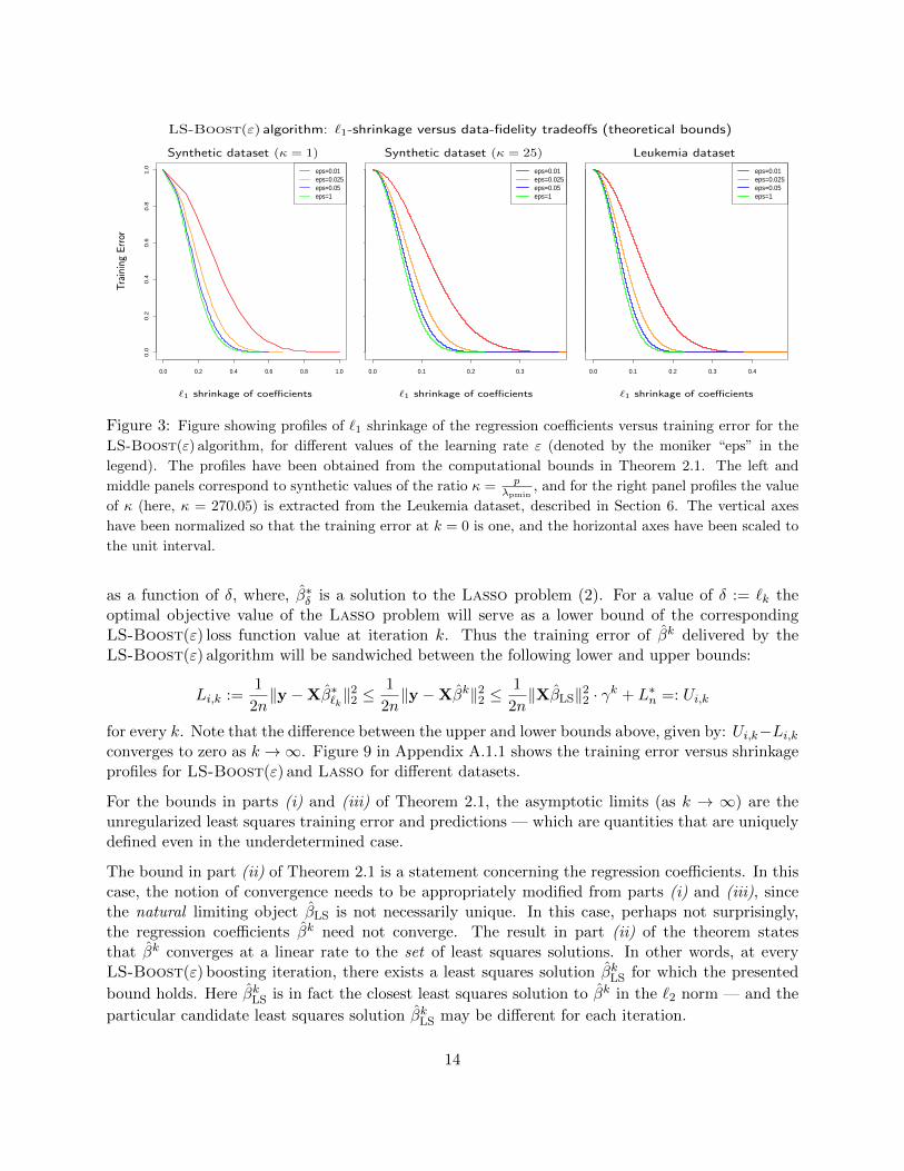
Figure 3: Figure showing profiles of `1 shrinkage of the regression coefficients versus training error for the

LS-Boost(ε) algorithm, for different values of the learning rate ε (denoted by the moniker “eps” in the

legend). The profiles have been obtained from the computational bounds in Theorem 2.1. The left and

middle panels correspond to synthetic values of the ratio κ = pλpmin

, and for the right panel profiles the value

of κ (here, κ = 270.05) is extracted from the Leukemia dataset, described in Section 6. The vertical axes

have been normalized so that the training error at k = 0 is one, and the horizontal axes have been scaled to

the unit interval.

as a function of δ, where, β∗δ is a solution to the Lasso problem (2). For a value of δ := `k theoptimal objective value of the Lasso problem will serve as a lower bound of the correspondingLS-Boost(ε) loss function value at iteration k. Thus the training error of βk delivered by theLS-Boost(ε) algorithm will be sandwiched between the following lower and upper bounds:

Li,k :=1

2n‖y −Xβ∗`k‖

22 ≤

1

2n‖y −Xβk‖22 ≤

1

2n‖XβLS‖22 · γk + L∗n =: Ui,k

for every k. Note that the difference between the upper and lower bounds above, given by: Ui,k−Li,kconverges to zero as k →∞. Figure 9 in Appendix A.1.1 shows the training error versus shrinkageprofiles for LS-Boost(ε) and Lasso for different datasets.

For the bounds in parts (i) and (iii) of Theorem 2.1, the asymptotic limits (as k → ∞) are theunregularized least squares training error and predictions — which are quantities that are uniquelydefined even in the underdetermined case.

The bound in part (ii) of Theorem 2.1 is a statement concerning the regression coefficients. In thiscase, the notion of convergence needs to be appropriately modified from parts (i) and (iii), sincethe natural limiting object βLS is not necessarily unique. In this case, perhaps not surprisingly,the regression coefficients βk need not converge. The result in part (ii) of the theorem statesthat βk converges at a linear rate to the set of least squares solutions. In other words, at everyLS-Boost(ε) boosting iteration, there exists a least squares solution βkLS for which the presented

bound holds. Here βkLS is in fact the closest least squares solution to βk in the `2 norm — and the

particular candidate least squares solution βkLS may be different for each iteration.

14

γ

λp

min

(XTX

)

p p

Figure 4: Figure showing the behavior of γ [left panel] and λpmin(XTX) [right panel] for different values

of ρ (denoted by the moniker “rho” in the legend) and p, with ε = 1. There are ten profiles in each panel

corresponding to different values of ρ for ρ = 0, 0.1, . . . , 0.9. Each profile documents the change in γ as a

function of p. Here, the data matrix X is comprised of n = 50 samples from a p-dimensional multivariate

Gaussian distribution with mean zero, and all pairwise correlations equal to ρ, and the features are then

standardized to have unit `2 norm. The left panel shows that γ exhibits a phase of rapid decay (as a

function of p) after which it stabilizes into the regime of fastest convergence. Interestingly, the behavior

shows a monotone trend in ρ: the rate of progress of LS-Boost(ε) becomes slower for larger values of ρ and

faster for smaller values of ρ.

Interpreting the parameters and algorithm dynamics There are several determinants ofthe quality of the bounds in the different parts of Theorem 2.1 which can be grouped into:

• algorithmic parameters: this includes the learning rate ε and the number of iterations k, and

• data dependent quantities: ‖XβLS‖2, λpmin(XTX), and p.

The coefficient of linear convergence is given by the quantity γ := 1− ε(2−ε)4κ(XTX)

, where κ(XTX) :=p

λpmin(XTX). Note that γ is monotone decreasing in ε for ε ∈ (0, 1], and is minimized at ε = 1.

This simple observation confirms the general intuition about LS-Boost(ε) : ε = 1 correspondsto the most aggressive model fitting behavior in the LS-Boost(ε) family, with smaller values of εcorresponding to a slower model fitting process. The ratio κ(XTX) is a close cousin of the conditionnumber associated with the data matrix X — and smaller values of κ(XTX) imply a faster rate ofconvergence.

In the overdetermined case with n ≥ p and rank(X) = p, the condition number κ(XTX) :=λmax(XTX)λmin(XTX)

plays a key role in determining the stability of the least-squares solution βLS and in

measuring the degree of multicollinearity present. Note that κ(XTX) ∈ [1,∞), and that theproblem is better conditioned for smaller values of this ratio. Furthermore, since rank(X) = p itholds that λpmin(XTX) = λmin(XTX), and thus κ(XTX) ≤ κ(XTX) by (9). Thus the conditionnumber κ(XTX) always upper bounds the classical condition number κ(XTX), and if λmax(XTX)is close to p, then κ(XTX) ≈ κ(XTX) and the two measures essentially coincide. Finally, since inthis setup βLS is unique, part (ii) of Theorem 2.1 implies that the sequence {βk} converges linearly

15

to the unique least squares solution βLS.

In the underdetermined case with p > n, λmin(XTX) = 0 and thus κ(XTX) = ∞. On the otherhand, κ(XTX) <∞ since λpmin(XTX) is the smallest nonzero (hence positive) eigenvalue of XTX.Therefore the condition number κ(XTX) is similar to the classical condition number κ(·) restrictedto the subspace S spanned by the columns of X (whose dimension is rank(X)). Interestingly,the linear rate of convergence enjoyed by LS-Boost(ε) is in a sense adaptive — the algorithmautomatically adjusts itself to the convergence rate dictated by the parameter γ “as if” it knowsthat the null space of X is not relevant.

Dynamics of the LS-Boost(ε) algorithm versus number of boosting iterations

ρ = 0 ρ = 0.5 ρ = 0.9

Sor

ted

Co

effici

ent

Ind

ices

Number of Boosting Iterations Number of Boosting Iterations Number of Boosting Iterations

Figure 5: Showing the LS-Boost(ε) algorithm run on the same synthetic dataset as was used in Figure 9,

with p = 500 and ε = 1, for three different values of the pairwise correlation ρ. A point is “on” if the

corresponding regression coefficient is updated at iteration k. Here the vertical axes have been reoriented so

that the coefficients that are updated the maximum number of times appear lower on the axes. For larger

values of ρ, we see that the LS-Boost(ε) algorithm aggressively updates the coefficients for a large number

of iterations, whereas the dynamics of the algorithm for smaller values of ρ are less pronounced. For larger

values of ρ the LS-Boost(ε) algorithm takes longer to reach the least squares fit and this is reflected in the

above figure from the update patterns in the regression coefficients. The dynamics of the algorithm evident

in this figure nicely complements the insights gained from Figure 1.

As the dataset is varied, the value of γ can change substantially from one dataset to another,thereby leading to differences in the convergence behavior bounds in parts (i)-(v) of Theorem 2.1.To settle all of these ideas, we can derive some simple bounds on γ using tools from random matrixtheory. Towards this end, let us suppose that the entries of X are drawn from a standard Gaussianensemble, which are subsequently standardized such that every column of X has unit `2 norm. Thenit follows from random matrix theory [43] that λpmin(XTX) ' 1

n(√p−√n)2 with high probability.

(See Appendix A.2.4 for a more detailed discussion of this fact.) To gain better insights into thebehavior of γ and how it depends on the values of pairwise correlations of the features, we performedsome computational experiments, the results of which are shown in Figure 4. Figure 4 shows thebehavior of γ as a function of p for a fixed n = 50 and ε = 1, for different datasets X simulatedas follows. We first generated a multivariate data matrix from a Gaussian distribution with mean

16

zero and covariance Σp×p = (σij), where, σij = ρ for all i 6= j; and then all of the columns of thedata matrix were standardized to have unit `2 norm. The resulting matrix was taken as X. Weconsidered different cases by varying the magnitude of pairwise correlations of the features ρ —when ρ is small, the rate of convergence is typically faster (smaller γ) and the rate becomes slower(higher γ) for higher values of ρ. Figure 4 shows that the coefficient of linear convergence γ is quiteclose to 1.0 — which suggests a slowly converging algorithm and confirms our intuition about thealgorithmic behavior of LS-Boost(ε) . Indeed, LS-Boost(ε) , like any other boosting algorithm,should indeed converge slowly to the unregularized least squares solution. The slowly convergingnature of the LS-Boost(ε) algorithm provides, for the first time, a precise theoretical justificationof the empirical observation made in [28] that stagewise regression is widely considered ineffectiveas a tool to obtain the unregularized least squares fit, as compared to other stepwise model fittingprocedures like Forward Stepwise regression (discussed in Section 1).

The above discussion sheds some interesting insight into the behavior of the LS-Boost(ε) algo-rithm. For larger values of ρ, the observed covariates tend to be even more highly correlated (sincep � n). Whenever a pair of features are highly correlated, the LS-Boost(ε) algorithm finds itdifficult to prefer one over the other and thus takes turns in updating both coefficients, therebydistributing the effects of a covariate to all of its correlated cousins. Since a group of correlatedcovariates are all competing to be updated by the LS-Boost(ε) algorithm, the progress made bythe algorithm in decreasing the loss function is naturally slowed down. In contrast, when ρ is small,the LS-Boost(ε) algorithm brings in a covariate and in a sense completes the process by doingthe exact line-search on that feature. This heuristic explanation attempts to explain the slowerrate of convergence of the LS-Boost(ε) algorithm for large values of ρ — a phenomenon that weobserve in practice and which is also substantiated by the computational guarantees in Theorem2.1. We refer the reader to Figures 1 and 5 which further illustrate the above justification. State-ment (v) of Theorem 2.1 provides upper bounds on the `1 shrinkage of the coefficients. Figure 3illustrates the evolution of the data-fidelity versus `1-shrinkage as obtained from the computationalbounds in Theorem 2.1. Some additional discussion and properties of LS-Boost(ε) are presentedin Appendix A.2.3.

3 Boosting Algorithms as Subgradient Descent

Roadmap In this section we present a new unifying framework for interpreting the three boostingalgorithms that were discussed in Section 1, namely FSε, its non-uniform learning rate extensionFSεk , and LS-Boost(ε). We show herein that all three algorithmic families can be interpretedas instances of the subgradient descent method of convex optimization, applied to the problem ofminimizing the largest correlation between residuals and predictors. Interestingly, this unifying lenswill also result in a natural generalization of FSε with very strong ties to the Lasso solutions, aswe will present in Sections 4 and 5. The framework presented in this section leads to convergenceguarantees for FSε and FSεk . In Theorem 3.1 herein, we present a theoretical description of theevolution of the FSε algorithm, in terms of its data-fidelity and shrinkage guarantees as a function ofthe number of boosting iterations. These results are a consequence of the computational guaranteesfor FSε that inform us about the rate at which the FSε training error, regression coefficients, andpredictions make their way to their least squares counterparts. In order to develop these results,we first motivate and briefly review the subgradient descent method of convex optimization.

17

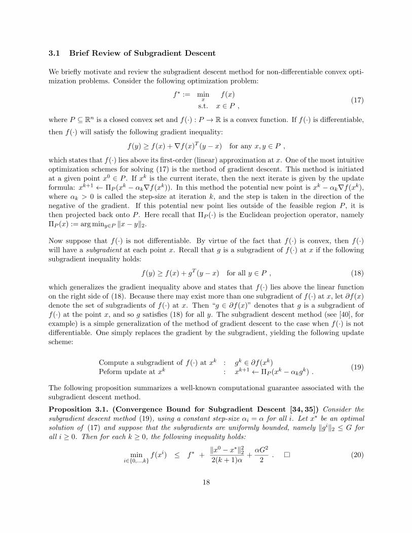
3.1 Brief Review of Subgradient Descent

We briefly motivate and review the subgradient descent method for non-differentiable convex opti-mization problems. Consider the following optimization problem:

f∗ := minx

f(x)

s.t. x ∈ P ,(17)

where P ⊆ Rn is a closed convex set and f(·) : P → R is a convex function. If f(·) is differentiable,

then f(·) will satisfy the following gradient inequality:

f(y) ≥ f(x) +∇f(x)T (y − x) for any x, y ∈ P ,

which states that f(·) lies above its first-order (linear) approximation at x. One of the most intuitiveoptimization schemes for solving (17) is the method of gradient descent. This method is initiatedat a given point x0 ∈ P . If xk is the current iterate, then the next iterate is given by the updateformula: xk+1 ← ΠP (xk − αk∇f(xk)). In this method the potential new point is xk − αk∇f(xk),where αk > 0 is called the step-size at iteration k, and the step is taken in the direction of thenegative of the gradient. If this potential new point lies outside of the feasible region P , it isthen projected back onto P . Here recall that ΠP (·) is the Euclidean projection operator, namelyΠP (x) := arg miny∈P ‖x− y‖2.

Now suppose that f(·) is not differentiable. By virtue of the fact that f(·) is convex, then f(·)will have a subgradient at each point x. Recall that g is a subgradient of f(·) at x if the followingsubgradient inequality holds:

f(y) ≥ f(x) + gT (y − x) for all y ∈ P , (18)

which generalizes the gradient inequality above and states that f(·) lies above the linear functionon the right side of (18). Because there may exist more than one subgradient of f(·) at x, let ∂f(x)denote the set of subgradients of f(·) at x. Then “g ∈ ∂f(x)” denotes that g is a subgradient off(·) at the point x, and so g satisfies (18) for all y. The subgradient descent method (see [40], forexample) is a simple generalization of the method of gradient descent to the case when f(·) is notdifferentiable. One simply replaces the gradient by the subgradient, yielding the following updatescheme:

Compute a subgradient of f(·) at xk : gk ∈ ∂f(xk)Peform update at xk : xk+1 ← ΠP (xk − αkgk) .

(19)

The following proposition summarizes a well-known computational guarantee associated with thesubgradient descent method.

Proposition 3.1. (Convergence Bound for Subgradient Descent [34, 35]) Consider thesubgradient descent method (19), using a constant step-size αi = α for all i. Let x∗ be an optimalsolution of (17) and suppose that the subgradients are uniformly bounded, namely ‖gi‖2 ≤ G forall i ≥ 0. Then for each k ≥ 0, the following inequality holds:

mini∈{0,...,k}

f(xi) ≤ f∗ +‖x0 − x∗‖222(k + 1)α

+αG2

2. (20)

18

The left side of (20) is simply the best objective function value obtained among the first k iterations.The right side of (20) bounds the best objective function value from above, namely the optimalvalue f∗ plus a nonnegative quantity that is a function of the number of iterations k, the constantstep-size {αi}, the bound G on the norms of subgradients, and the distance from the initial point toan optimal solution x∗ of (17). Note that for a fixed step-size α > 0, the right side of (20) goes toαG2

2 as k →∞. In the interest of completeness, we include a proof of Proposition 3.1 in AppendixA.3.1.

3.2 A Subgradient Descent Framework for Boosting

We now show that the boosting algorithms discussed in Section 1, namely FSε and its relativesFSεk and LS-Boost(ε), can all be interpreted as instantiations of the subgradient descent methodto minimize the largest absolute correlation between the residuals and predictors.

Let Pres := {r ∈ Rn : r = y−Xβ for some β ∈ Rp} denote the affine space of residuals and considerthe following convex optimization problem:

Correlation Minimization (CM) : f∗ := minr

f(r) := ‖XT r‖∞s.t. r ∈ Pres ,

(21)

which we dub the “Correlation Minimization” problem, or CM for short. Note an importantsubtlety in the CM problem, namely that the optimization variable in CM is the residual r and notthe regression coefficient vector β.

Since the columns of X have unit `2 norm by assumption, f(r) is the largest absolute correlationbetween the residual vector r and the predictors. Therefore (21) is the convex optimization problemof minimizing the largest correlation between the residuals and the predictors, over all possiblevalues of the residuals. From (6) with r = y − Xβ we observe that XT r = 0 if and only if βis a least squares solution, whereby f(r) = ‖XT r‖∞ = 0 for the least squares residual vectorr = rLS = y −XβLS. Since the objective function in (21) is nonnegative, we conclude that f∗ = 0and the least squares residual vector rLS is also the unique optimal solution of the CM problem(21). Thus CM can be viewed as an optimization problem which also produces the least squaressolution.

The following proposition states that the three boosting algorithms FSε, FSεk and LS-Boost(ε)can all be viewed as instantiations of the subgradient descent method to solve the CM problem(21).

Proposition 3.2. Consider the subgradient descent method (19) with step-size sequence {αk} tosolve the correlation minimization (CM) problem (21), initialized at r0 = y. Then:

(i) the FSε algorithm is an instance of subgradient descent, with a constant step-size αk := ε ateach iteration,

(ii) the FSεk algorithm is an instance of subgradient descent, with non-uniform step-sizes αk := εkat iteration k, and

19

(iii) the LS-Boost(ε) algorithm is an instance of subgradient descent, with non-uniform step-sizesαk := ε|ujk | at iteration k, where ujk := arg minu ‖rk −Xjku‖22.

Proof. We first prove (i). Recall the update of the residuals in FSε:

rk+1 = rk − ε · sgn((rk)TXjk)Xjk .

We first show that gk := sgn((rk)TXjk)Xjk is a subgradient of the objective function f(r) =‖XT r‖∞ of the correlation minimization problem CM (21) at r = rk. At iteration k, FSε choosesthe coefficient to update by selecting jk ∈ arg max

j∈{1,...,p}|(rk)TXj |, whereby

sgn((rk)TXjk)((rk)TXjk

)= ‖XT (rk)‖∞, and therefore for any r it holds that:

f(r) = ‖XT r‖∞ ≥ sgn((rk)TXjk)((Xjk)T r

)= sgn((rk)TXjk)

((Xjk)T (rk + r − rk)

)= ‖XT (rk)‖∞ + sgn((rk)TXjk)

((Xjk)T (r − rk)

)= f(rk) + sgn((rk)TXjk)

((Xjk)T (r − rk)

).

Therefore using the definition of a subgradient in (18), it follows that gk := sgn((rk)TXjk)Xjk is asubgradient of f(r) = ‖XT r‖∞ at r = rk. Therefore the update rk+1 = rk − ε · sgn((rk)TXjk)Xjk

is of the form rk+1 = rk − εgk where gk ∈ ∂f(rk). Last of all notice that the update can also bewritten as rk−εgk = rk+1 = y−Xβk+1 ∈ Pres, hence ΠPres(r

k−εgk) = rk−εgk, i.e., the projectionstep is superfluous here, and therefore rk+1 = ΠPres(r

k− εgk), which is precisely the update for thesubgradient descent method with step-size αk := ε.

The proof of (ii) is the same as (i) with a step-size choice of αk = εk at iteration k. Furthermore,as discussed in Section 1, LS-Boost(ε) may be thought of as a specific instance of FSεk , wherebythe proof of (iii) follows as a special case of (ii).

Proposition 3.2 presents a new interpretation of the boosting algorithms FSε and its cousins as sub-gradient descent. This is interesting especially since FSε and LS-Boost(ε) have been traditionallyinterpreted as greedy coordinate descent or steepest descent type procedures [25,28]. This has thefollowing consequences of note:

• We take recourse to existing tools and results about subgradient descent optimization toinform us about the computational guarantees of these methods. When translated to thesetting of linear regression, these results will shed light on the data fidelity vis-a-vis shrinkagecharacteristics of FSε and its cousins — all using quantities that can be easily obtained priorto running the boosting algorithm. We will show the details of this in Theorem 3.1 below.

• The subgradient optimization viewpoint provides a unifying algorithmic theme which we willalso apply to a regularized version of problem CM (21), and that we will show is very stronglyconnected to the Lasso. This will be developed in Section 4. Indeed, the regularized versionof the CM problem that we will develop in Section 4 will lead to a new family of boostingalgorithms which are a seemingly minor variant of the basic FSε algorithm but deliver (O(ε)-approximate) solutions to the Lasso.

20

3.3 Deriving and Interpreting Computational Guarantees for FSε

The following theorem presents the convergence properties of FSε, which are a consequence of theinterpretation of FSε as an instance of the subgradient descent method.

Theorem 3.1. (Convergence Properties of FSε) Consider the FSε algorithm with learningrate ε. Let k ≥ 0 be the total number of iterations. Then there exists an index i ∈ {0, . . . , k} forwhich the following bounds hold:

(i) (training error): Ln(βi)− L∗n ≤p

2nλpmin(XTX)

[‖XβLS‖22ε(k+1) + ε

]2

(ii) (regression coefficients): there exists a least squares solution βiLS such that:

‖βi − βiLS‖2 ≤√p

λpmin(XTX)

[‖XβLS‖22ε(k + 1)

+ ε

]

(iii) (predictions): for every least-squares solution βLS it holds that

‖Xβi −XβLS‖2 ≤√p√

λpmin(XTX)

[‖XβLS‖22ε(k + 1)

+ ε

]

(iv) (correlation values) ‖XT ri‖∞ ≤‖XβLS‖222ε(k + 1)

+ε

2

(v) (`1-shrinkage of coefficients): ‖βi‖1 ≤ kε

(vi) (sparsity of coefficients): ‖βi‖0 ≤ k .

The proof of Theorem 3.1 is presented in Appendix A.3.2.

Interpreting the Computational Guarantees Theorem 3.1 accomplishes for FSε what The-orem 2.1 did for LS-Boost(ε) — parts (i) – (iv) of the theorem describe the rate in which thetraining error, regression coefficients, and related quantities make their way towards their (O(ε)-approximate) unregularized least squares counterparts. Part (v) of the theorem also describes therate at which the shrinkage of the regression coefficients evolve as a function of the number of boost-ing iterations. The rate of convergence of FSε is sublinear, unlike the linear rate of convergence forLS-Boost(ε) . Note that this type of sublinear convergence implies that the rate of decrease ofthe training error (for instance) is dramatically faster in the very early iterations as compared tolater iterations. Taken together, Theorems 3.1 and 2.1 highlight an important difference betweenthe behavior of algorithms LS-Boost(ε) and FSε:

• the limiting solution of the LS-Boost(ε) algorithm (as k → ∞) corresponds to the unregu-larized least squares solution, but

• the limiting solution of the FSε algorithm (as k → ∞) corresponds to an O(ε) approximateleast squares solution.

21

FSε algorithm: `1 shrinkage versus data-fidelity tradeoffs (theoretical bounds)

Synthetic dataset (κ = 1) Leukemia dataset Leukemia dataset (zoomed)

Tra

inin

gE

rror

0.00 0.05 0.10 0.15 0.20 0.25 0.30

0.0

00

.05

0.1

00

.15

0.2

00

.25

0.3

0

eps=1eps=0.05eps=0.025eps=0.01

0.00 0.02 0.04 0.06 0.08 0.100

.00

0.0

20

.04

0.0

60

.08

0.1

0

eps=1eps=0.05eps=0.025eps=0.01

0.000 0.002 0.004 0.006 0.008 0.010

0.0

00

.02

0.0

40

.06

0.0

80

.10

eps=1eps=0.05eps=0.025eps=0.01

`1 shrinkage of coefficients `1 shrinkage of coefficients `1 shrinkage of coefficients

Figure 6: Figure showing profiles of `1 shrinkage bounds of the regression coefficients versus training error

bounds for the FSε algorithm, for different values of the learning rate ε. The profiles have been obtained

from the bounds in parts (i) and (v) of Theorem 3.1. The left panel corresponds to a hypothetical dataset

using κ = pλpmin

= 1, and the middle and right panels use the parameters of the Leukemia dataset.

As demonstrated in Theorems 2.1 and 3.1, both LS-Boost(ε) and FSε have nice convergence prop-erties with respect to the unconstrained least squares problem (4). However, unlike the convergenceresults for LS-Boost(ε) in Theorem 2.1, FSε exhibits a sublinear rate of convergence towards asuboptimal least squares solution. For example, part (i) of Theorem 3.1 implies in the limit ask →∞ that FSε identifies a model with training error at most:

L∗n +pε2

2n(λpmin(XTX)). (22)

In addition, part (ii) of Theorem 3.1 implies that as k →∞, FSε identifies a model whose distance

to the set of least squares solutions {βLS : XTXβLS = XTy} is at most:ε√p

λpmin(XTX).

Note that the computational guarantees in Theorem 3.1 involve the quantities λpmin(XTX) and

‖XβLS‖2, assuming n and p are fixed. To settle ideas, let us consider the synthetic datasets usedin Figures 4 and 1, where the covariates were generated from a multivariate Gaussian distributionwith pairwise correlation ρ. Figure 4 suggests that λpmin(XTX) decreases with increasing ρ values.Thus, controlling for other factors appearing in the computational bounds4 , it follows from thestatements of Theorem 3.1 that the training error decreases much more rapidly for smaller ρ values,as a function of k. This is nicely validated by the computational results in Figure 1 (the three toppanel figures), which show that the training errors decay at a faster rate for smaller values ofρ.

Let us examine more carefully the properties of the sequence of models explored by FSε and thecorresponding tradeoffs between data fidelity and model complexity. Let TBound and SBound

4To control for other factors, for example, we may assume that p > n and for different values of ρ we have‖XβLS‖2 = ‖y‖2 = 1 with ε fixed across the different examples.

22

denote the training error bound and shrinkage bound in parts (i) and (v) of Theorem 3.1, respec-tively. Then simple manipulation of the arithmetic in these two bounds yields the following tradeoffequation:

TBound =p

2nλpmin(XTX)

[‖XβLS‖22

SBound + ε+ ε

]2

.

The above tradeoff between the training error bound and the shrinkage bound is illustrated inFigure 6, which shows this tradeoff curve for four different values of the learning rate ε. Exceptfor very small shrinkage levels, lower values of ε produce smaller training errors. But unlike thecorresponding tradeoff curves for LS-Boost(ε) , there is a range of values of the shrinkage for whichsmaller values of ε actually produce larger training errors, though admittedly this range is for verysmall shrinkage values. For more reasonable shrinkage values, smaller values of ε will correspondto smaller values of the training error.

Part (v) of Theorems 2.1 and 3.1 presents shrinkage bounds for FSε and LS-Boost(ε) , respectively.Let us briefly compare these bounds. Examining the shrinkage bound for LS-Boost(ε) , we canbound the left term from above by

√k√ε‖XβLS‖2. We can also bound the right term from above

by ε‖XβLS‖2/(1−√γ) where recall from Section 2 that γ is the linear convergence rate coefficient

γ := 1− ε(2−ε)λpmin(XTX)4p . We may therefore alternatively write the following shrinkage bound for

LS-Boost(ε) :

‖βk‖1 ≤ ‖XβLS‖2 min{√

k√ε , ε/(1−√γ)

}. (23)

The shrinkage bound for FSε is simply kε. Comparing these two bounds, we observe that not onlydoes the shrinkage bound for FSε grow at a faster rate as a function of k for large enough k, but alsothe shrinkage bound for FSε grows unbounded in k, unlike the right term above for the shrinkagebound of LS-Boost(ε) .

One can also compare FSε and LS-Boost(ε) in terms of the efficiency with which these two methodsachieve a certain pre-specified data-fidelity. In Appendix A.3.3 we show, at least in theory, thatLS-Boost(ε) is much more efficient than FSε at achieving such data-fidelity, and furthermore itdoes so with much better shrinkage.

4 Regularized Correlation Minimization, Boosting, and Lasso

Roadmap In this section we introduce a new boosting algorithm, parameterized by a scalarδ ≥ 0, which we denote by R-FSε,δ (for Regularized incremental Forward Stagewise regression),that is obtained by incorporating a simple rescaling step to the coefficient updates in FSε. We thenintroduce a regularized version of the Correlation Minimization (CM) problem (21) which we referto as RCM. We show that the adaptation of the subgradient descent algorithmic framework to theRegularized Correlation Minimization problem RCM exactly yields the algorithm R-FSε,δ. Thenew algorithm R-FSε,δ may be interpreted as a natural extension of popular boosting algorithmslike FSε, and has the following notable properties:

23

• Whereas FSε updates the coefficients in an additive fashion by adding a small amount εto the coefficient most correlated with the current residuals, R-FSε,δ first shrinks all of thecoefficients by a scaling factor 1− ε

δ < 1 and then updates the selected coefficient in the sameadditive fashion as FSε.

• R-FSε,δ delivers O(ε)-accurate solutions to the Lasso in the limit as k → ∞, unlike FSεwhich delivers O(ε)-accurate solutions to the unregularized least squares problem.

• R-FSε,δ has computational guarantees similar in spirit to the ones described in the context ofFSε – these quantities directly inform us about the data-fidelity vis-a-vis shrinkage tradeoffsas a function of the number of boosting iterations and the learning rate ε.

The notion of using additional regularization along with the implicit shrinkage imparted by boostingis not new in the literature. Various interesting notions have been proposed in [10, 14, 22, 26, 45],see also the discussion in Appendix A.4.4 herein. However, the framework we present here is new.We present a unified subgradient descent framework for a class of regularized CM problems thatresults in algorithms that have appealing structural similarities with forward stagewise regressiontype algorithms, while also being very strongly connected to the Lasso.

Boosting with additional shrinkage – R-FSε,δ Here we give a formal description of theR-FSε,δ algorithm. R-FSε,δ is controlled by two parameters: the learning rate ε, which plays thesame role as the learning rate in FSε, and the “regularization parameter” δ ≥ ε. Our reasonfor referring to δ as a regularization parameter is due to the connection between R-FSε,δ and theLasso, which will be made clear later. The shrinkage factor, i.e., the amount by which we shrinkthe coefficients before updating the selected coefficient, is determined as 1− ε

δ . Supposing that wechoose to update the coefficient indexed by jk at iteration k, then the coefficient update may bewritten as:

βk+1 ←(1− ε

δ

)βk + ε · sgn((rk)TXjk)ejk .

Below we give a concise description of R-FSε,δ, including the update for the residuals that corre-sponds to the update for the coefficients stated above.

Algorithm: R-FSε,δ

Fix the learning rate ε > 0, regularization parameter δ > 0 such that ε ≤ δ, and number ofiterations M .

Initialize at r0 = y, β0 = 0, k = 0.

1. For 0 ≤ k ≤M do the following:

2. Compute: jk ∈ arg maxj∈{1,...,p}

|(rk)TXj |

3. rk+1 ← rk − ε[sgn((rk)TXjk)Xjk + 1

δ (rk − y)]

βk+1jk←(1− ε

δ

)βkjk + ε sgn((rk)TXjk) and βk+1

j ←(1− ε

δ

)βkj , j 6= jk

Note that R-FSε,δ and FSε are structurally very similar – and indeed when δ =∞ then R-FSε,δ isexactly FSε. Note also that R-FSε,δ shares the same upper bound on the sparsity of the regression

24

coefficients as FSε, namely for all k it holds that: ‖βk‖0 ≤ k. When δ < ∞ then, as previouslymentioned, the main structural difference between R-FSε,δ and FSε is the additional rescaling ofthe coefficients by the factor 1− ε

δ . This rescaling better controls the growth of the coefficients and,as will be demonstrated next, plays a key role in connecting R-FSε,δ to the Lasso.

Regularized Correlation Minimization (RCM) and Lasso The starting point of our formalanalysis of R-FSε,δ is the Correlation Minimization (CM) problem (21), which we now modify byintroducing a regularization term that penalizes residuals that are far from the vector of observationsy. This modification leads to the following parametric family of optimization problems indexed byδ ∈ (0,∞]:

RCMδ : f∗δ := minr

fδ(r) := ‖XT r‖∞ + 12δ‖r − y‖22

s.t. r ∈ Pres := {r ∈ Rn : r = y −Xβ for some β ∈ Rp} ,(24)

where “RCM” connotes Regularlized Correlation Minimization. Note that RCM reduces to thecorrelation minimization problem CM (21) when δ =∞. RCM may be interpreted as the problemof minimizing, over the space of residuals, the largest correlation between the residuals and thepredictors plus a regularization term that penalizes residuals that are far from the response y(which itself can be interpreted as the residuals associated with the model β = 0).

Interestingly, as we show in Appendix A.4.1, RCM (24) is equivalent to the Lasso (2) via du-ality. This equivalence provides further insight about the regularization used to obtain RCMδ.Comparing the Lasso and RCM, notice that the space of the variables of the Lasso is the spaceof regression coefficients β, namely Rp, whereas the space of the variables of RCM is the space ofmodel residuals, namely Rn, or more precisely Pres. The duality relationship shows that RCMδ (24)is an equivalent characterization of the Lasso problem, just like the correlation minimization (CM)problem (21) is an equivalent characterization of the (unregularized) least squares problem. Recallthat Proposition 3.2 showed that subgradient descent applied to the CM problem (24) (which isRCMδ with δ = ∞) leads to the well-known boosting algorithm FSε. We now extend this themewith the following Proposition, which demonstrates R-FSε,δ is equivalent to subgradient descentapplied to RCMδ.

Proposition 4.1. The R-FSε,δ algorithm is an instance of subgradient descent to solve the regular-ized correlation minimization (RCMδ) problem (24), initialized at r0 = y, with a constant step-sizeαk := ε at each iteration.

The proof of Proposition 4.1 is presented in Appendix A.4.2.

4.1 R-FSε,δ: Computational Guarantees and their Implications

In this subsection we present computational guarantees and convergence properties of the boostingalgorithm R-FSε,δ. Due to the structural equivalence between R-FSε,δ and subgradient descentapplied to the RCMδ problem (24) (Proposition 4.1) and the close connection between RCMδ

and the Lasso (Appendix A.4.1), the convergence properties of R-FSε,δ are naturally stated withrespect to the Lasso problem (2). Similar to Theorem 3.1 which described such properties for

25

FSε (with respect to the unregularized least squares problem), we have the following properties forR-FSε,δ.

Theorem 4.1. (Convergence Properties of R-FSε,δ for the Lasso ) Consider the R-FSε,δalgorithm with learning rate ε and regularization parameter δ ∈ (0,∞), where ε ≤ δ. Then theregression coefficient βk is feasible for the Lasso problem (2) for all k ≥ 0. Let k ≥ 0 denote aspecific iteration counter. Then there exists an index i ∈ {0, . . . , k} for which the following boundshold:

(i) (training error): Ln(βi)− L∗n,δ ≤δn

[‖XβLS‖222ε(k+1) + 2ε

](ii) (predictions): for every Lasso solution β∗δ it holds that

‖Xβi −Xβ∗δ‖2 ≤

√δ‖XβLS‖22ε(k + 1)

+ 4δε

(iii) (`1-shrinkage of coefficients): ‖βi‖1 ≤ δ[1−

(1− ε

δ

)k] ≤ δ

(iv) (sparsity of coefficients): ‖βi‖0 ≤ k .

The proof of Theorem 4.1 is presented in Appendix A.4.3.

R-FSε,δ algorithm, Prostate cancer dataset (computational bounds)

` 1-n

orm

ofco

effici

ents

(rel

ativ

esc

ale)

Tra

inin

gE

rror

(rel

ativ

esc

ale)

Iterations Iterations Iterations

Figure 7: Figure showing the evolution of the R-FSε,δ algorithm (with ε = 10−4) for different values of

δ, as a function of the number of boosting iterations for the Prostate cancer dataset, with n = 10, p = 44,

appearing in the bottom panel of Figure 8. [Left panel] shows the change of the `1-norm of the regression

coefficients. [Middle panel] shows the evolution of the training errors, and [Right panel] is a zoomed-in

version of the middle panel. Here we took different values of δ given by δ = frac× δmax, where, δmax denotes

the `1-norm of the minimum `1-norm least squares solution, for 7 different values of frac.

Interpreting the Computational Guarantees The statistical interpretations implied by thecomputational guarantees presented in Theorem 4.1 are analogous to those previously discussed for

26

LS-Boost(ε) (Theorem 2.1) and FSε (Theorem 3.1). These guarantees inform us about the data-fidelity vis-a-vis shrinkage tradeoffs as a function of the number of boosting iterations, as nicelydemonstrated in Figure 7. There is, however, an important differentiation between the propertiesof R-FSε,δ and the properties of LS-Boost(ε) and FSε, namely:

• For LS-Boost(ε) and FSε, the computational guarantees (Theorems 2.1 and 3.1) describehow the estimates make their way to a unregularized (O(ε)-approximate) least squares solu-tion as a function of the number of boosting iterations.

• For R-FSε,δ, our results (Theorem 4.1) characterize how the estimates approach a (O(ε)-approximate) Lasso solution.

Notice that like FSε, R-FSε,δ traces out a profile of regression coefficients. This is reflected in item(iii) of Theorem 4.1 which bounds the `1-shrinkage of the coefficients as a function of the numberof boosting iterations k. Due to the rescaling of the coefficients, the `1-shrinkage may be boundedby a geometric series that approaches δ as k grows. Thus, there are two important aspects of thebound in item (iii): (a) the dependence on the number of boosting iterations k which characterizesmodel complexity during early iterations, and (b) the uniform bound of δ which applies even inthe limit as k →∞ and implies that all regression coefficient iterates βk are feasible for the Lassoproblem (2).

On the other hand, item (i) characterizes the quality of the coefficients with respect to the Lassosolution, as opposed to the unregularized least squares problem as in FSε. In the limit as k →∞,item (i) implies that R-FSε,δ identifies a model with training error at most L∗n,δ + 2δε

n . This upperbound on the training error may be set to any prescribed error level by appropriately tuning ε; inparticular, for ε ≈ 0 and fixed δ > 0 this limit is essentially L∗n,δ. Thus, combined with the uniformbound of δ on the `1-shrinkage, we see that the R-FSε,δ algorithm delivers the Lasso solution inthe limit as k →∞.

It is important to emphasize that R-FSε,δ should not just be interpreted as an algorithm to solvethe Lasso. Indeed, like FSε, the trajectory of the algorithm is important and R-FSε,δ may identifya more statistically interesting model in the interior of its profile. Thus, even if the Lasso solutionfor δ leads to overfitting, the R-FSε,δ updates may visit a model with better predictive performanceby trading off bias and variance in a more desirable fashion suitable for the particular problem athand.

Figure 8 shows the profiles of R-FSε,δ for different values of δ ≤ δmax, where δmax is the `1-norm ofthe minimum `1-norm least squares solution. Curiously enough, Figure 8 shows that in some cases,the profile of R-FSε,δ bears a lot of similarities with that of the Lasso (as presented in Figure 2).However, the profiles are in general different. Indeed, R-FSε,δ imposes a uniform bound of δ onthe `1-shrinkage, and so for values larger than δ we cannot possibly expect R-FSε,δ to approximatethe Lasso path. However, even if δ is taken to be sufficiently large (but finite) the profiles maybe different. In this connection it is helpful to draw the analogy between the curious similaritiesbetween the FSε (i.e., R-FSε,δ with δ =∞) and Lasso coefficient profiles, even though the profilesare different in general.

As a final note, we point out that one can also interpret R-FSε,δ as the Frank-Wolfe algorithm inconvex optimization applied to the Lasso (2) in line with [2]. We refer the reader to AppendixA.4.5 for discussion of this point.

27

FSε R-FSε,δ, δ = 0.99δmax R-FSε,δ,δ = 0.91δmax R-FSε,δ,δ = 0.81δmaxR

egre

ssio

nC

oeffi

cien

ts

FSε R-FSε,δ, δ = 0.44δmax R-FSε,δ,δ = 0.37δmax R-FSε,δ,δ = 0.33δmax

Reg

ress

ion

Co

effici

ents

`1-norm of coefficients `1-norm of coefficients `1-norm of coefficients `1-norm of coefficients

Figure 8: Coefficient profiles for R-FSε,δ as a function of the `1-norm of the regression coefficients, for the

same datasets appearing in Figure 2. For each example, different values of δ have been considered. The

left panel corresponds to the choice δ = ∞, i.e., FSε. In all the above cases, the algorithms were run for

a maximum of 100,000 boosting iterations with ε = 10−4. [Top Panel] Corresponds to the Prostate cancer

dataset with n = 98 and p = 8. All the coefficient profiles look similar, and they all seem to coincide with

the Lasso profile (see also Figure 2). [Bottom Panel] Shows the Prostate cancer dataset with a subset

of samples n = 10 with all interactions included with p = 44. The coefficient profiles in this example are

sensitive to the choice of δ and are seen to be more constrained towards the end of the path, for decreasing

δ values. The profiles are different than the Lasso profiles, as seen in Figure 2. The regression coefficients

at the end of the path correspond to approximate Lasso solutions, for the respective values of δ.

5 A Modified Forward Stagewise Algorithm for Computing theLasso Path

In Section 4 we introduced the boosting algorithm R-FSε,δ (which is a very close cousin of FSε)that delivers solutions to the Lasso problem (2) for a fixed but arbitrary δ, in the limit as k →∞with ε ≈ 0. Furthermore, our experiments in Section 6 suggest that R-FSε,δ may lead to estimatorswith good statistical properties for a wide range of values of δ, provided that the value of δ is nottoo small. While R-FSε,δ by itself may be considered as a regularization scheme with excellentstatistical properties, the boosting profile delivered by R-FSε,δ might in some cases be differentfrom the Lasso coefficient profile, as we saw in Figure 8. Therefore in this section we investigate

28

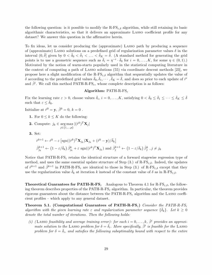
the following question: is it possible to modify the R-FSε,δ algorithm, while still retaining its basicalgorithmic characteristics, so that it delivers an approximate Lasso coefficient profile for anydataset? We answer this question in the affirmative herein.

To fix ideas, let us consider producing the (approximate) Lasso path by producing a sequenceof (approximate) Lasso solutions on a predefined grid of regularization parameter values δ in theinterval (0, δ] given by 0 < δ0 < δ1 < . . . < δK = δ. (A standard method for generating the gridpoints is to use a geometric sequence such as δi = η−i · δ0 for i = 0, . . . ,K, for some η ∈ (0, 1).)Motivated by the notion of warm-starts popularly used in the statistical computing literature inthe context of computing a path of Lasso solutions (55) via coordinate descent methods [23], wepropose here a slight modification of the R-FSε,δ algorithm that sequentially updates the value ofδ according to the predefined grid values δ0, δ1, · · · , δK = δ, and does so prior to each update of ri

and βi. We call this method PATH-R-FSε, whose complete description is as follows:

Algorithm: PATH-R-FSε

Fix the learning rate ε > 0, choose values δi, i = 0, . . . ,K, satisfying 0 < δ0 ≤ δ1 ≤ · · · ≤ δK ≤ δsuch that ε ≤ δ0.

Initialize at r0 = y, β0 = 0, k = 0 .

1. For 0 ≤ k ≤ K do the following:

2. Compute: jk ∈ arg maxj∈{1,...,p}

|(rk)TXj |

3. Set:

rk+1 ← rk − ε[sgn((rk)TXjk)Xjk + (rk − y)/δk

]βk+1jk←(1− ε/δk

)βkjk + ε sgn((rk)TXjk) and βk+1

j ←(1− ε/δk

)βkj , j 6= jk

Notice that PATH-R-FSε retains the identical structure of a forward stagewise regression type ofmethod, and uses the same essential update structure of Step (3.) of R-FSε,δ. Indeed, the updates

of rk+1 and βk+1 in PATH-R-FSε are identical to those in Step (3.) of R-FSε,δ except that theyuse the regularization value δk at iteration k instead of the constant value of δ as in R-FSε,δ.

Theoretical Guarantees for PATH-R-FSε Analogous to Theorem 4.1 for R-FSε,δ, the follow-ing theorem describes properties of the PATH-R-FSε algorithm. In particular, the theorem providesrigorous guarantees about the distance between the PATH-R-FSε algorithm and the Lasso coeffi-cient profiles – which apply to any general dataset.

Theorem 5.1. (Computational Guarantees of PATH-R-FSε) Consider the PATH-R-FSεalgorithm with the given learning rate ε and regularization parameter sequence {δk}. Let k ≥ 0denote the total number of iterations. Then the following holds:

(i) (Lasso feasibility and average training error): for each i = 0, . . . , k, βi provides an approxi-mate solution to the Lasso problem for δ = δi. More specifically, βi is feasible for the Lassoproblem for δ = δi, and satisfies the following suboptimality bound with respect to the entire

29

boosting profile:

1

k + 1

k∑i=0

(Ln(βi)− L∗n,δi

)≤ δ‖XβLS‖22

2nε(k + 1)+

2δε

n

(ii) (`1-shrinkage of coefficients): ‖βi‖1 ≤ δi for i = 0, . . . , k.

(iii) (sparsity of coefficients): ‖βi‖0 ≤ i for i = 0, . . . , k.

Corollary 5.1. (PATH-R-FSε approximates the Lasso path) For every fixed ε > 0 andk →∞ it holds that:

lim supk→∞

1

k + 1

k∑i=0

(Ln(βi)− L∗n,δi

)≤ 2δε

n,

(and the quantity on the right side of the above bound goes to zero as ε→ 0).

The proof of Theorem 5.1 is presented in Appendix A.5.1.

Interpreting the computational guarantees Let us now provide some interpretation of theresults stated in Theorem 5.1. Recall that Theorem 4.1 presented bounds on the distance betweenthe training errors achieved by the boosting algorithm R-FSε,δ and Lasso training errors for a fixedbut arbitrary δ that is specified a priori. The message in Theorem 5.1 generalizes this notion to afamily of Lasso solutions corresponding to a grid of δ values. The theorem thus quantifies how theboosting algorithm PATH-R-FSε simultaneously approximates a path of Lasso solutions.

Part (i) of Theorem 5.1 first implies that the sequence of regression coefficient vectors {βi} is feasiblealong the Lasso path, for the Lasso problem (2) for the sequence of regularization parameter values{δi}. In considering guarantees with respect to the training error, we would ideally like guaranteesthat hold across the entire spectrum of {δi} values. While part (i) does not provide such strongguarantees, part (i) states that these quantities will be sufficiently small on average. Indeed, fora fixed ε and as k → ∞, part (i) states that the average of the differences between the training

errors produced by the algorithm and the optimal training errors is at most 2δεn . This non-vanishing

bound (for ε > 0) is a consequence of the fixed learning rate ε used in PATH-R-FSε – such boundswere also observed for R-FSε,δ and FSε.

Thus on average, the training error of the model βi will be sufficiently close (as controlled by thelearning rate ε) to the optimal training error for the corresponding regularization parameter valueδi. In summary, while PATH-R-FSε provides the most amount of flexibility in terms of controllingfor model complexity since it allows for any (monotone) sequence of regularization parameter valuesin the range (0, δ], this freedom comes at the cost of weaker training error guarantees with respect toany particular δi value (as opposed to R-FSε,δ which provides strong guarantees with respect to thefixed value δ). Nevertheless, part (i) guarantees that the training errors will be sufficiently small onaverage across the entire path of regularization parameter values explored by the algorithm.

30

6 Some Computational Experiments

We consider an array of examples exploring statistical properties of the different boosting algorithmsstudied herein. We consider different types of synthetic and real datasets, which are briefly describedhere.

Synthetic datasets We considered synthetically generated datasets of the following types:

• Eg-A. Here the data matrix X is generated from a multivariate normal distribution, i.e., foreach i = 1, . . . , n, xi ∼ MVN(0,Σ). Here xi denotes the ith row of X and Σ = (σij) ∈ Rp×phas all off-diagonal entries equal to ρ and all diagonal entries equal to one. The response

y ∈ Rn is generated as y = Xβpop + ε, where εiiid∼ N(0, σ2). The underlying regression

coefficient was taken to be sparse with βpopi = 1 for all i ≤ 5 and βpop

i = 0 otherwise. σ2 ischosen so as to control the signal to noise ratio SNR := Var(x′β)/σ2.

Different values of SNR, n, p and ρ were taken and they have been specified in our resultswhen and where appropriate.

• Eg-B. Here the datasets are generated similar to above, with βpopi = 1 for i ≤ 10 and βpop

i = 0otherwise. We took the value of SNR=1in this example.

Real datasets We considered four different publicly available microarray datasets as describedbelow.

• Leukemia dataset. This dataset, taken from [12], was processed to have n = 72 andp = 500. y was created as y = Xβpop + ε; with βpop

i = 1 for all i ≤ 10 and zero otherwise.

• Golub dataset. This dataset, taken from the R package mpm, was processed to have n = 73and p = 500, with artificial responses generated as above.

• Khan dataset. This dataset, taken from the website of [28], was processed to have n = 73and p = 500, with artificial responses generated as above.

• Prostate dataset. This dataset, analyzed in [15], was processed to create three types ofdifferent datasets: (a) the original dataset with n = 97 and p = 8, (b) a dataset with n = 97and p = 44, formed by extending the covariate space to include second order interactions,and (c) a third dataset with n = 10 and p = 44, formed by subsampling the previous dataset.

For more detail on the above datasets, we refer the reader to the Appendix B.

Note that in all the examples we standardized X such that the columns have unit `2 norm, beforerunning the different algorithms studied herein.

6.1 Statistical properties of boosting algorithms: an empirical study

We performed some experiments to better understand the statistical behavior of the different boost-ing methods described in this paper. We summarize our findings here; for details (including tables,figures and discussions) we refer the reader to Appendix, Section B.

31

Sensitivity of the Learning Rate in LS-Boost(ε) and FSε We explored how the trainingand test errors for LS-Boost(ε) and FSε change as a function of the number of boosting iterationsand the learning rate. We observed that the best predictive models were sensitive to the choice ofε—the best models were obtained at values larger than zero and smaller than one. When comparedto Lasso , stepwise regression [15] and FS0 [15]; FSε and LS-Boost(ε) were found to be as goodas the others, in some cases the better than the rest.

Statistical properties of R-FSε,δ, Lasso and FSε: an empirical study We performed someexperiments to evaluate the performance of R-FSε,δ, in terms of predictive accuracy and sparsityof the optimal model, versus the more widely known methods FSε and Lasso. We found thatwhen δ was larger than the best δ for the Lasso (in terms of obtaining a model with the bestpredictive performance), R-FSε,δ delivered a model with excellent statistical properties – R-FSε,δled to sparse solutions and the predictive performance was as good as, and in some cases betterthan, the Lasso solution. We observed that the choice of δ does not play a very crucial role inthe R-FSε,δ algorithm, once it is chosen to be reasonably large; indeed the number of boostingiterations play a more important role. The best models delivered by R-FSε,δ were more sparse thanFSε.

Acknowledgements

The authors will like to thank Alexandre Belloni, Jerome Friedman, Trevor Hastie, Arian Malekiand Tomaso Poggio for helpful discussions and encouragement. A preliminary unpublished versionof some of the results herein was posted on the ArXiv [18].

References

[1] M. Avriel. Nonlinear Programming Analysis and Methods. Prentice-Hall, Englewood Cliffs, N.J., 1976.

[2] F. Bach. Duality between subgradient and conditional gradient methods. SIAM Journal on Optimiza-tion, 25(1):115–129, Jan. 2015.

[3] D. Bertsekas. Nonlinear Programming. Athena Scientific, Belmont, MA, 1999.

[4] S. Boyd and L. Vandenberghe. Convex Optimization. Cambridge University Press, Cambridge, 2004.

[5] L. Breiman. Arcing classifiers (with discussion). Annals of Statistics, 26:801–849, 1998.

[6] L. Breiman. Prediction games and arcing algorithms. Neural Computation, 11(7):1493–1517, 1999.

[7] P. Buhlmann. Boosting for high-dimensional linear models. The Annals of Statistics, pages 559–583,2006.

[8] P. Buhlmann and T. Hothorn. Boosting algorithms: regularization, prediction and model fitting (withdiscussion). Statistical Science, 22(4):477–505, 2008.

[9] P. Buhlmann and B. Yu. Boosting with the l2 loss: regression and classification. Journal of the AmericanStatistical Association, 98(462):324–339, 2003.

[10] P. Buhlmann and B. Yu. Sparse boosting. The Journal of Machine Learning Research, 7:1001–1024,2006.

32

[11] K. Clarkson. Coresets, sparse greedy approximation, and the Frank-Wolfe algorithm. 19th ACM-SIAMSymposium on Discrete Algorithms, pages 922–931, 2008.

[12] M. Dettling and P. Buhlmann. Boosting for tumor classification with gene expression data. Bioinfor-matics, 19(9):1061–1069, 2003.

[13] D. L. Donoho, I. M. Johnstone, G. Kerkyacharian, and D. Picard. Wavelet shrinkage: asymptopia?Journal of the Royal Statistical Society. Series B (Methodological), pages 301–369, 1995.

[14] J. Duchi and Y. Singer. Boosting with structural sparsity. In Proceedings of the 26th Annual Interna-tional Conference on Machine Learning, pages 297–304. ACM, 2009.

[15] B. Efron, T. Hastie, I. Johnstone, and R. Tibshirani. Least angle regression (with discussion). Annalsof Statistics, 32(2):407–499, 2004.

[16] M. Frank and P. Wolfe. An algorithm for quadratic programming. Naval Research Logistics Quarterly,3:95–110, 1956.

[17] R. M. Freund and P. Grigas. New analysis and results for the Frank-Wolfe method. to appear inMathematical Programming, 2014.

[18] R. M. Freund, P. Grigas, and R. Mazumder. Adaboost and forward stagewise regression are first-orderconvex optimization methods. CoRR, abs/1307.1192, 2013.

[19] Y. Freund. Boosting a weak learning algorithm by majority. Information and computation, 121(2):256–285, 1995.

[20] Y. Freund and R. Schapire. Experiments with a new boosting algorithm. In Machine Learning: Pro-ceedings of the Thirteenth International Conference, pages 148–156. Morgan Kauffman, San Francisco,1996.

[21] J. Friedman. Greedy function approximation: A gradient boosting machine. Annals of Statistics,29(5):1189–1232, 2001.

[22] J. Friedman. Fast sparse regression and classification. Technical report, Department of Statistics,Stanford University, 2008.

[23] J. Friedman, T. Hastie, H. Hoefling, and R. Tibshirani. Pathwise coordinate optimization. Annals ofApplied Statistics, 2(1):302–332, 2007.

[24] J. Friedman, T. Hastie, and R. Tibshirani. Additive logistic regression: a statistical view of boosting(with discussion). Annals of Statistics, 28:337–307, 2000.

[25] J. H. Friedman. Greedy function approximation: A gradient boosting machine. Annals of Statistics,29:1189–1232, 2000.

[26] J. H. Friedman and B. E. Popescu. Importance sampled learning ensembles. Journal of MachineLearning Research, 94305, 2003.

[27] T. Hastie, J. Taylor, R. Tibshirani, and G. Walther. Forward stagewise regression and the monotonelasso. Electronic Journal of Statistics, 1:1–29, 2007.

[28] T. Hastie, R. Tibshirani, and J. Friedman. Elements of Statistical Learning: Data Mining, Inference,and Prediction. Springer Verlag, New York, 2009.

[29] T. J. Hastie and R. J. Tibshirani. Generalized additive models, volume 43. CRC Press, 1990.

[30] M. Jaggi. Revisiting Frank-Wolfe: Projection-free sparse convex optimization. In Proceedings of the30th International Conference on Machine Learning (ICML-13), pages 427–435, 2013.

[31] S. G. Mallat and Z. Zhang. Matching pursuits with time-frequency dictionaries. Signal Processing,IEEE Transactions on, 41(12):3397–3415, 1993.

33

[32] L. Mason, J. Baxter, P. Bartlett, and M. Frean. Boosting algorithms as gradient descent. 12:512–518,2000.

[33] A. Miller. Subset selection in regression. CRC Press Washington, 2002.

[34] Y. E. Nesterov. Introductory lectures on convex optimization: a basic course, volume 87 of AppliedOptimization. Kluwer Academic Publishers, Boston, 2003.

[35] B. Polyak. Introduction to Optimization. Optimization Software, Inc., New York, 1987.

[36] G. Ratsch, T. Onoda, and K.-R. Muller. Soft margins for adaboost. Machine learning, 42(3):287–320,2001.

[37] S. Rosset, J. Zhu, and T. Hastie. Boosting as a regularized path to a maximum margin classifier.Journal of Machine Learning Research, 5:941–973, 2004.

[38] R. Schapire. The strength of weak learnability. Machine Learning, 5(2):197–227, 1990.

[39] R. Schapire and Y. Freund. Boosting: Foundations and Algorithms. Adaptive computation and machinelearning. Mit Press, 2012.

[40] N. Z. Shor. Minimization Methods for Non-Differentiable Functions, volume 3 of Springer Series inComputational Mathematics. Springer, Berlin, 1985.

[41] R. Tibshirani. Regression shrinkage and selection via the lasso. Journal of the Royal Statistical Society,Series B, 58(1):267–288, 1996.

[42] J. Tukey. Exploratory data analysis. Addison-Wesley,Massachusetts, 1977.

[43] R. Vershynin. Introduction to the non-asymptotic analysis of random matrices. arXiv preprintarXiv:1011.3027, 2010.

[44] S. Weisberg. Applied Linear Regression. Wiley, New York, 1980.

[45] P. Zhao and B. Yu. Stagewise lasso. The Journal of Machine Learning Research, 8:2701–2726, 2007.

34

A Technical Details and Supplementary Material

A.1 Additional Details for Section 1

A.1.1 Figure showing Training error versus `1-shrinkage bounds

Figure 9 showing profiles of `1 norm of the regression coefficients versus training error for LS-Boost(ε) , FSε and Lasso.

`1 shrinkage versus data-fidelity tradeoffs: LS-Boost(ε) , FSε, and Lasso

Tra

inin

gE

rror

`1 shrinkage of coefficients `1 shrinkage of coefficients `1 shrinkage of coefficients

Figure 9: Figure showing profiles of `1 norm of the regression coefficients versus training error for LS-

Boost(ε) , FSε and Lasso. [Left panel] Shows profiles for a synthetic dataset where the covariates are

drawn from a Gaussian distribution with pairwise correlations ρ = 0.5. The true β has ten non-zeros with

βi = 1 for i = 1, . . . , 10, and SNR = 1. Here we ran LS-Boost(ε) with ε = 1 and ran FSε with ε = 10−2.

The middle (and right) panel profiles corresponds to the Prostate cancer dataset (described in Section 6).

Here we ran LS-Boost(ε) with ε = 0.01 and we ran FSε with ε = 10−5. The right panel figure is a zoomed-in

version of the middle panel in order to highlight the difference in profiles between LS-Boost(ε) , FSε and

Lasso. The vertical axes have been normalized so that the training error at k = 0 is one, and the horizontal

axes have been scaled to the unit interval (to express the `1-norm of βk as a fraction of the maximum).

A.2 Additional Details for Section 2

A.2.1 Properties of Convex Quadratic Functions

Consider the following quadratic optimization problem (QP) defined as:

h∗ := minx∈Rn

h(x) := 12x

TQx+ qTx+ qo ,

where Q is a symmetric positive semi-definite matrix, whereby h(·) is a convex function. We assumethat Q 6= 0, and recall that λpmin(Q) denotes the smallest nonzero (and hence positive) eigenvalueof Q.

35

Proposition A.1. If h∗ > −∞, then for any given x, there exists an optimal solution x∗ of (QP)for which

‖x− x∗‖2 ≤

√2(h(x)− h∗)λpmin(Q)

.

Also, it holds that

‖∇h(x)‖2 ≥√λpmin(Q) · (h(x)− h∗)

2.

Proof: The result is simply manipulation of linear algebra. Let us assume without loss of generalitythat qo = 0. If h∗ > −∞, then (QP) has an optimal solution x∗, and the set of optimal solutionsare characterized by the gradient condition

0 = ∇h(x) = Qx+ q .

Now let us write the sparse eigendecomposition of Q as Q = PDP T where D is a diagonal matrixof non-zero eigenvalues of Q and the columns of P are orthonormal, namely P TP = I. Because(QP) has an optimal solution, the system of equations Qx = −q has a solution, and let x denoteany such solution. Direct manipulation establishes:

PP T q = −PP TQx = −PP TPDP T x = −PDP T x = −Qx = q .

Furthermore, let x := −PD−1P T q. It is then straightforward to see that x is an optimal solutionof (QP) since in particular:

Qx = −PDP TPD−1P T q = −PP T q = −q ,

and hence

h∗ = 12 x

TQx+ qT x = −12 x

TQx = −12qTPD−1P TPDP TPD−1P T q = −1

2qTPD−1P T q .

Now let x be given, and define x∗ := [I−PP T ]x−PD−1P T q. Then just as above it is straightforwardto establish that Qx∗ = −q whereby x∗ is an optimal solution. Furthermore, it holds that:

‖x− x∗‖22 = (qTPD−1 + xTP )P TP (D−1P T q + P Tx)

= (qTPD−12 + xTPD

12 )D−1(D−

12P T q +D

12P Tx)

≤ 1λpmin(Q)(qTPD−

12 + xTPD

12 )(D−

12P T q +D

12P Tx)

= 1λpmin(Q)(qTPD−1P T q + xTPDP Tx+ 2xTPP T q)

= 1λpmin(Q)(−2h∗ + xTQx+ 2xT q)

= 2λpmin(Q)(h(x)− h∗) ,

and taking square roots establishes the first inequality of the proposition.

36

Using the gradient inequality for convex functions, it holds that:

h∗ = h(x∗) ≥ h(x) +∇h(x)T (x∗ − x)

≥ h(x)− ‖∇h(x)‖2‖x∗ − x‖2

≥ h(x)− ‖∇h(x)‖2√

2(h(x)−h∗)λpmin(Q) ,

and rearranging the above proves the second inequality of the proposition.

A.2.2 Proof of Theorem 2.1

We first prove part (i). Utilizing (12), which states that rk+1 = rk − ε((rk)TXjk

)Xjk , we

have:Ln(βk+1) = 1

2n‖rk+1‖22

= 12n‖r

k − ε((rk)TXjk

)Xjk‖22

= 12n‖r

k‖22 − 1nε((rk)TXjk

)2+ 1

2nε2((rk)TXjk

)2= Ln(βk)− 1

2nε(2− ε)((rk)TXjk

)2= Ln(βk)− 1

2nε(2− ε)n2‖∇Ln(βk)‖2∞ ,

(25)

(where the last equality above uses (11)), which yields:

Ln(βk+1)− L∗n = Ln(βk)− L∗n − n2 ε(2− ε)‖∇Ln(βk)‖2∞ . (26)

We next seek to bound the right-most term above. We will do this by invoking Proposition A.1,which presents two important properties of convex quadratic functions. Because Ln(·) is a convexquadratic function of the same format as Proposition A.1 with h(·) ← Ln(·), Q ← 1

nXTX, andh∗ ← L∗n, it follows from the second property of Proposition A.1 that

‖∇Ln(β)‖2 ≥

√λpmin( 1

nXTX)(Ln(β)− L∗n)

2=

√λpmin(XTX)(Ln(β)− L∗n)

2n.

Therefore

‖∇Ln(β)‖2∞ ≥ 1p‖∇Ln(β)‖22 ≥

λpmin(XTX)(Ln(β)− L∗n)

2np.

Substituting this inequality into (26) yields after rearranging:

Ln(βk+1)− L∗n ≤ (Ln(βk)− L∗n)

(1− ε(2− ε)λpmin(XTX)

4p

)= (Ln(βk)− L∗n) · γ . (27)

Now note that Ln(β0) = Ln(0) = 12n‖y‖

22 and

Ln(β0)−L∗n = 12n‖y‖

22− 1

2n‖y−XβLS‖22 = 12n‖y‖

22− 1

2n(‖y‖22−2yTXβLS+‖XβLS‖22) = 12n‖XβLS‖22 ,

37

where the last equality uses the normal equations (6). Then (i) follows by using elementary induc-tion and combining the above with (27):

Ln(βk)− L∗n ≤ (Ln(β0)− L∗n) · γk = 12n‖XβLS‖22 · γk .

To prove (ii), we invoke the first inequality of Proposition A.1, which in this context statesthat

‖βk − βLS‖2 ≤

√2(Ln(βk)− L∗n)√λpmin( 1

nXTX)=

√2n(Ln(βk)− L∗n)√λpmin(XTX)

.

Part (ii) then follows by substituting the bound on (Ln(βk)− L∗n) from (i) and simplifying terms.

Similarly, the proof of (iii) follows from the observation that ‖Xβk−XβLS‖2 =

√2n(Ln(βk)− L∗n)

and then substituting the bound on (Ln(βk)− L∗n) from (i) and simplifying terms.

To prove (iv), define the point βk := βk + ujkejk . Then using similar arithmetic as in (25) oneobtains:

L∗n ≤ Ln(βk) = Ln(βk)− 12n u

2jk,

where we recall that ujk = (rk)TXjk . This inequality then rearranges to

|ujk | ≤√

2n(Ln(βk)− L∗n) ≤ ‖XβLS‖2 · γk/2 , (28)

where the second inequality follows by substituting the bound on (Ln(βi)−L∗n) from (i). Recalling(7) and (11), the above is exactly part (iv).

Part (v) presents two distinct bounds on ‖βk‖1, which we prove independently. To prove the firstbound, let βLS be any least-squares solution, which therefore satisfies (6). It is then elementary toderive using similar manipulation as in (25) that for all i the following holds:

‖X(βi+1 − βLS)‖22 = ‖X(βi − βLS)‖22 − (2ε− ε2)u2ji (29)

which implies that

(2ε− ε2)k−1∑i=0

u2ji = ‖X(β0 − βLS)‖22 − ‖X(βk − βLS)‖22 = ‖XβLS‖22 − ‖X(βk − βLS)‖22 . (30)

Then note that

‖βk‖1 ≤ ‖(εuj0 , . . . , εujk−1)‖1 ≤

√kε‖(uj0 , . . . , ujk−1

)‖2 =√k√

ε2−ε

√‖XβLS‖22 − ‖XβLS −Xβk‖22 ,

where the last equality is from (30).

To prove the second bound in (v), noting that βk =∑k−1

i=0 εujieji , we bound ‖βk‖1 as follows:

‖βk‖1 ≤ εk−1∑i=0

|uji | ≤ ε‖XβLS‖2k−1∑i=0

γi/2

=ε‖XβLS‖2

1−√γ

(1− γk/2

),

38

where the second inequality uses (28) for each i ∈ {0, . . . , k−1} and the final equality is a geometricseries, which completes the proof of (v). Part (vi) is simply the property of LS-Boost(ε) thatderives from the fact that β0 := 0 and at every iteration at most one coordinate of β changes statusfrom a zero to a non-zero value.

A.2.3 Additional properties of LS-Boost(ε)

We present two other interesting properties of the LS-Boost(ε) algorithm, namely an additionalbound on the correlation between residuals and predictors, and a bound on the `2-shrinkage of theregression coefficients. Both are presented in the following proposition.

Proposition A.2. (Two additional properties of LS-Boost(ε)) Consider the iterates of theLS-Boost(ε) algorithm after k iterations and consider the linear convergence rate coefficient γ:

γ :=

(1− ε(2− ε)λpmin(XTX)

4p

).

(i) There exists an index i ∈ {0, . . . , k} for which the `∞ norm of the gradient vector of the leastsquares loss function evaluated at βi satisfies:

‖∇Ln(βi)‖∞ = 1n‖X

T ri‖∞ ≤ min

√‖XβLS‖22 − ‖XβLS −Xβk+1‖22

n√ε(2− ε)(k + 1)

, 1n‖XβLS‖2 · γ

k/2

. (31)

(ii) Let J` denote the number of iterations of LS-Boost(ε) , among the first k iterations, where thealgorithm takes a step in coordinate `, for ` = 1, . . . , p, and let Jmax := max{J1, . . . , Jp}. Then the

following bound on the shrinkage of βk holds:

‖βk‖2 ≤√Jmax

√ε

2− ε

√‖XβLS‖22 − ‖XβLS −Xβk‖22 . (32)

Proof. We first prove part (i). The first equality of (31) is a restatement of (11). For eachi ∈ {0, . . . , k}, recall that uji = (ri)TXji and that |uji | = |(ri)TXji | = ‖XT ri‖∞, from (11).Therefore:(

mini∈{0,...,k}

|uji |)2

= mini∈{0,...,k}

u2ji ≤

1

k + 1

k∑i=0

u2ji ≤

‖XβLS‖22 − ‖X(βk+1 − βLS)‖22ε(2− ε)(k + 1)

, (33)

where the final inequality follows from (30) in the proof of Theorem 2.1. Now letting i be an indexachieving the minimum in the left hand side of the above and taking square roots implies that

‖XT ri‖∞ = |uji | ≤

√‖XβLS‖22 − ‖XβLS −Xβk+1‖22√

ε(2− ε)(k + 1),

39

which is equivalent to the inequality in (31) for the first right-most term therein. Directly applying(28) from the proof of Theorem 2.1 and using the fact that i is an index achieving the minimum inthe left hand side of (33) yields:

‖XT ri‖∞ = |uji | ≤ |ujk | ≤ ‖XβLS‖2(

1− ε(2− ε)λpmin(XTX)

4p

)k/2,

which is equivalent to the inequality in (31) for the second right-most term therein.

We now prove part (ii). For fixed k > 0, let J (`) denote the set of iteration counters whereLS-Boost(ε) modifies coordinate ` of β, namely

J (`) := {i : i < k and ji = ` in Step (2.) of Algorithm LS-Boost(ε) } ,

for ` = 1, . . . , p. Then J` = |J (`)|, and the sets J (1), . . . ,J (p) partition the iteration index set{0, 1, . . . , k − 1}. We have:

‖βk‖2 ≤ ‖(∑

i∈J (1) εuji , . . . ,∑

i∈J (p) εuji)‖2

≤∥∥∥(√J(1)

√∑i∈J (1) ε

2u2ji, . . . ,

√J(p)

√∑i∈J (p) ε

2u2ji

)∥∥∥2

≤ ε√Jmax

∥∥∥(√∑i∈J (1) u2ji, . . . ,

√∑i∈J (p) u

2ji

)∥∥∥2

= ε√Jmax

√(u2j0

+ . . .+ u2jk−1

),

(34)

and the proof is completed by applying inequality (30).

Part (i) of Proposition A.2 describes the behavior of the gradient of the least squares loss func-tion — indeed, recall that the dynamics of the gradient are closely linked to that of the LS-Boost(ε) algorithm and, in particular, to the evolution of the loss function values. To illustratethis connection, let us recall two simple characteristics of the LS-Boost(ε) algorithm:

Ln(βk)− Ln(βk+1) = n2 ε(2− ε)‖∇Ln(βk)‖2∞

rk+1 − rk = −ε((rk)TXjk

)Xjk ,

which follow from (26) and Step (3.) of the FSε algorithm respectively. The above updates ofthe LS-Boost(ε) algorithm clearly show that smaller values of the `∞ norm of the gradient slowsdown the “progress” of the residuals and thus the overall algorithm. Larger values of the norm ofthe gradient, on the other hand, lead to rapid “progress” in the algorithm. Here, we use the term“progress” to measure the amount of decrease in training error and the norm of the changes insuccessive residuals. Informally speaking, the LS-Boost(ε) algorithm operationally works towardsminimizing the unregularized least squares loss function — and the gradient of the least squaresloss function is simultaneously shrunk towards zero. Equation (31) precisely quantifies the rate atwhich the `∞ norm of the gradient converges to zero. Observe that the bound is a minimum of twodistinct rates: one which decays as O( 1√

k) and another which is linear with parameter

√γ. This is

40

similar to item (v) of Theorem 2.1. For small values of k the first rate will dominate, until a pointis reached where the linear rate begins to dominate. Note that the dependence on the linear rateγ suggests that for large values of correlations among the samples, the gradient decays slower thanfor smaller pairwise correlations among the samples.

The behavior of the LS-Boost(ε) algorithm described above should be contrasted with the FSεalgorithm. In view of Step (3.) of the FSε algorithm, the successive differences of the residuals inFSε are indifferent to the magnitude of the gradient of the least squares loss function — as longas the gradient is non-zero, then for FSε it holds that ‖rk+1 − rk‖2 = ε. Thus FSε undergoes amore erratic evolution, unlike LS-Boost(ε) where the convergence of the residuals is much more“smooth.”

A.2.4 Concentration Results for λpmin(XTX) in the High-dimensional Case

Proposition A.3. Suppose that p > n, let X ∈ Rn×p be a random matrix whose entries are i.i.d.standard normal random variables, and define X := 1√

nX. Then, it holds that:

E[λpmin(XTX)] ≥ 1

n

(√p−√n)2

.

Furthermore, for every t ≥ 0, with probability at least 1− 2 exp(−t2/2), it holds that:

λpmin(XTX) ≥ 1

n

(√p−√n− t

)2.

Proof. Let σ1(XT ) ≥ σ2(XT ) ≥ . . . ≥ σn(XT ) denote the ordered singular values of XT (equiva-lently of X). Then, Theorem 5.32 of [43] states that:

E[σn(XT )] ≥ √p−√n ,

which thus implies:

E[λpmin(XTX)] = E[(σn(XT ))2] ≥ (E[σn(XT )])2 =1

n(E[σn(XT )])2 ≥ 1

n

(√p−√n)2

,

where the first inequality is Jensen’s inequality.

Corollary 5.35 of [43] states that, for every t ≥ 0, with probability at least 1−2 exp(−t2/2) it holdsthat:

σn(XT ) ≥ √p−√n− t ,

which implies that:

λpmin(XTX) = (σn(XT ))2 =1

n(σn(XT ))2 ≥ 1

n

(√p−√n− t

)2.

Note that, in practice, we standardize the model matrix X so that its columns have unit `2 norm.Supposing that the entries of X did originate from an i.i.d. standard normal matrix X, standardiz-ing the columns of X is not equivalent to setting X := 1√

nX. But, for large enough n, standardizing

is a valid approximation to normalizing by 1√n

, i.e., X ≈ 1√nX, and we may thus apply the above

results.

41

A.3 Additional Details for Section 3

A.3.1 An Elementary Sequence Process Result, and a Proof of Proposition 3.1

Consider the following elementary sequence process: x0 ∈ Rn is given, and xi+1 ← xi − αigi forall i ≥ 0, where gi ∈ Rn and αi is a nonnegative scalar, for all i. For this process there are noassumptions on how the vectors gi might be generated.

Proposition A.4. For the elementary sequence process described above, suppose that the {gi} areuniformly bounded, namely ‖gi‖2 ≤ G for all i ≥ 0. Then for all k ≥ 0 and for any x ∈ Rn it holdsthat:

1∑ki=0 αi

k∑i=0

αi(gi)T (xi − x) ≤

‖x0 − x‖22 +G2∑k

i=0 α2i

2∑k

i=0 αi. (35)

Indeed, in the case when αi = ε for all i, it holds that:

1

k + 1

k∑i=0

(gi)T (xi − x) ≤ ‖x0 − x‖222(k + 1)ε

+G2ε

2. (36)

Proof. Elementary arithmetic yields the following:

‖xi+1 − x‖22 = ‖xi − αigi − x‖22

= ‖xi − x‖22 + α2i ‖gi‖22 + 2αi(g

i)T (x− xi)

≤ ‖xi − x‖22 +G2α2i + 2αi(g

i)T (x− xi) .

Rearranging and summing these inequalities for i = 0, . . . , k then yields:

2

k∑i=0

αi(gi)T (xi − x) ≤ G2

k∑i=0

α2i + ‖x0 − x‖22 − ‖xk+1 − x‖22 ≤ G2

k∑i=0

α2i + ‖x0 − x‖22 ,

which then rearranges to yield (35). (36) follows from (35) by direct substitution.

Proof of Proposition 3.1: Consider the subgradient descent method (19) with arbitrary step-sizesαi for all i. We will prove the following inequality:

mini∈{0,...,k}

f(xi) ≤ f∗ +‖x0 − x∗‖22 +G2

∑ki=0 α

2i

2∑k

i=0 αi, (37)

from which the proof of Proposition 3.1 follows by substituting αi = α for all i and simplifyingterms. Let us now prove (37). The subgradient descent method (19) is applied to instances ofproblem (17) where f(·) is convex, and where gi is subgradient of f(·) at xi, for all i. If x∗ is anoptimal solution of (17), it therefore holds from the subgradient inequality that

f∗ = f(x∗) ≥ f(xi) + (gi)T (x− xi) .

42

Substituting this inequality in (35) for the value of x = x∗ yields:

‖x0 − x∗‖22 +G2∑k

i=0 α2i

2∑k

i=0 αi≥ 1∑k

i=0 αi

k∑i=0

αi(gi)T (xi − x∗)

≥ 1∑ki=0 αi

k∑i=0

αi(f(xi)− f∗) ≥ mini∈{0,...,k}

f(xi) .

A.3.2 Proof of Theorem 3.1

We first prove part (i). Note that item (i) of Proposition 3.2 shows that FSε is a specific instance ofsubgradient descent to solve problem (21), using the constant step-size ε. Therefore we can apply thecomputational guarantees associated with the subgradient descent method, particularly Proposition3.1, to the FSε algorithm. Examining Proposition 3.1, we need to work out the corresponding valuesof f∗, ‖x0−x∗‖2, α, and G in the context of FSε for solving the CM problem (21). Note that f∗ = 0for problem (21). We bound the distance from the initial residuals to the optimal least-squaresresiduals as follows:

‖r0 − r∗‖2 = ‖r0 − rLS‖2 = ‖y − (y −XβLS)‖2 = ‖XβLS‖2 .

From Proposition 3.2 part (i) we have α = ε. Last of all, we need to determine an upper bound Gon the norms of subgradients. We have:

‖gk‖2 = ‖sgn((rk)TXjk)Xjk‖2 = ‖Xjk‖2 = 1 ,

since the covariates have been standardized, so we can set G = 1. Now suppose algorithm FSε isrun for k iterations. Proposition 3.1 then implies that:

mini∈{0,...,k}

‖XT ri‖∞ = mini∈{0,...,k}

f(ri) ≤ f∗ +‖r0 − r∗‖222α(k + 1)

+αG2

2=‖XβLS‖222ε(k + 1)

+ε

2. (38)

The above inequality provides a bound on the best (among the first k residual iterates) empiricalcorrelation between between the residuals ri and each predictor variable, where the bound dependsexplicitly on the learning rate ε and the number of iterations k. Furthermore, invoking (7), theabove inequality implies the following upper bound on the norm of the gradient of the least squaresloss Ln(·) for the model iterates {βi} generated by FSε:

mini∈{0,...,k}

‖∇Ln(βi)‖∞ ≤‖XβLS‖22

2nε(k + 1)+

ε

2n. (39)

Let i be the index where the minimum is attained on the left side of the above inequality. Ina similar vein as in the analysis in Section 2, we now use Proposition A.1 which presents twoimportant properties of convex quadratic functions. Because Ln(·) is a convex quadratic function

43

of the same format as Proposition A.1 with h(·) ← Ln(·), Q ← 1nXTX, and h∗ ← L∗n, it follows

from the second property of Proposition A.1 that

‖∇Ln(βi)‖2 ≥

√λpmin( 1

nXTX)(Ln(βi)− L∗n)

2=

√λpmin(XTX)(Ln(βi)− L∗n)

2n,

where recall that λpmin(XTX) denotes the smallest non-zero (hence positive) eigenvalue of XTX.Therefore

‖∇Ln(βi)‖2∞ ≥ 1p‖∇Ln(βi)‖22 ≥

λpmin(XTX)(Ln(βi)− L∗n)

2np.

Substituting this inequality into (39) for the index i where the minimum is attained yields afterrearranging:

Ln(βi)− L∗n ≤p

2nλpmin(XTX)

[‖XβLS‖22ε(k + 1)

+ ε

]2

, (40)

which proves part (i). The proof of part (ii) follows by noting from the first inequality of PropositionA.1 that there exists a least-squares solution β∗ for which:

‖β∗ − βi‖2 ≤

√2(Ln(βi)− L∗n)

λpmin

(1nXTX

) =

√2n(Ln(βi)− L∗n)

λpmin(XTX)≤

√p

λpmin(XTX)

[‖XβLS‖22ε(k + 1)

+ ε

],

where the second inequality in the above chain follows using (40). The proof of part (iii) follows

by first observing that ‖X(βi − βLS)‖2 =

√2n(Ln(βi)− L∗n) and then substituting the bound on

(Ln(βi) − L∗n) from part (i) and simplifying terms. Part (iv) is a restatement of inequality (38).Finally, parts (v) and (vi) are simple and well-known structural properties of FSε that are re-statedhere for completeness.

A.3.3 A deeper investigation of the computational guarantees for LS-Boost(ε) andFSε

Here we show that in theory, LS-Boost(ε) is much more efficient than FSε if the primary goal isto obtain a model with a certain (pre-specified) data-fidelity. To formalize this notion, we considera parameter τ ∈ (0, 1]. We say that β is at a τ -relative distance to the least squares predictions ifβ satisfies:

‖Xβ −XβLS‖2 ≤ τ‖XβLS‖2 . (41)

Now let us pose the following question: if both LS-Boost(ε) and FSε are allowed to run withan appropriately chosen learning rate ε for each algorithm, which algorithm will satisfy (41) infewer iterations? We will answer this question by studying closely the computational guaranteesof Theorems 2.1 and 3.1. Since our primary goal is to compute β satisfying (41), we may optimizethe learning rate ε, for each algorithm, to achieve this goal with the smallest number of boostingiterations.

Let us first study LS-Boost(ε) . As we have seen, a learning rate of ε = 1 achieves the fastestrate of linear convergence for LS-Boost(ε) and is thus optimal with regard to the bound in part

44

(iii) of Theorem 2.1. If we run LS-Boost(ε) with ε = 1 for kLS-Boost(ε) :=⌈

4pλpmin(XTX)

ln(

1τ2

)⌉iterations, then it follows from part (iii) of Theorem 2.1 that we achieve (41). Furthermore, itfollows from (23) that the resulting `1-shrinkage bound will satisfy:

SboundLS-Boost(ε) ≤ ‖XβLS‖2√kLS-Boost(ε) .

For FSε, if one works out the arithmetic, the optimal number of boosting iterations to achieve (41)

is given by: kFSε :=⌈

4pλpmin(XTX)

(1τ2

)⌉− 1 using the learning rate ε = ‖XβLS‖2√

kFSε+1. Also, it follows

from part (v) of Theorem 3.1 that the resulting shrinkage bound will satisfy:

SboundFSε ≤ ε · kFSε ≈ ‖XβLS‖2 ·√kFSε .

Observe that kLS-Boost(ε) < kFSε , whereby LS-Boost(ε) is able to achieve (41) in fewer iterationsthan FSε. Indeed, if we let η denote the ratio kLS-Boost(ε) /kFSε , then it holds that

η :=kLS-Boost(ε)

kFSε≈

ln(

1τ2

)1τ2

≤ 1

e< 0.368 . (42)

The left panel of Figure 10 shows the value of η as a function of τ . For small values of thetolerance parameter τ we see that η is itself close to zero, which means that LS-Boost(ε) will needsignificantly fewer iterations than FSε to achieve the condition (41).

We can also examine the `1-shrinkage bounds similarly. If we let ϑ denote the ratio of

SboundLS-Boost(ε) to SboundFSε , then it holds that

ϑ :=SboundLS-Boost(ε)

SboundFSε=

√kLS-Boost(ε)

kFSε=

√ln(

1τ2

)1τ

≤ 1√e< 0.607 . (43)

This means that if both bounds are relatively tight, then the `1-shrinkage of the final model pro-duced by LS-Boost(ε) is smaller than that of the final model produced by FSε, by at least a factorof 0.607. The right panel of Figure 10 shows the value of ϑ as a function of τ . For small values ofthe relative predication error constant τ we see that ϑ is itself close to zero.

We summarize the above analysis in the following remark.

Remark A.1. (Comparison of efficiency of LS-Boost(ε) and FSε) Suppose that the primarygoal is to achieve a τ -relative prediction error as defined in (41), and that LS-Boost(ε) and FSεare run with appropriately determined learning rates for each algorithm. Then the ratio of requirednumber of iterations of these methods to achieve (41) satisfies

η :=kLS-Boost(ε)

kFSε< 0.368 .

45

η

0.0 0.2 0.4 0.6 0.8 1.0

0.0

0.2

0.4

0.6

0.8

1.0

tau

eta ϑ

0.0 0.2 0.4 0.6 0.8 1.0

0.0

0.2

0.4

0.6

0.8

1.0

tau

sqrt(

eta)

τ τ

Figure 10: Plot showing the value of the ratio η of iterations of LS-Boost(ε) to FSε (equation (42)) versus

the target relative prediction error τ [left panel], and the ratio ϑ of shrinkage bounds of LS-Boost(ε) to

FSε (equation (43)) versus the target relative prediction error τ [right panel].

Also, the ratio of the shrinkage bounds from running these numbers of iterations satisfies

ϑ :=SboundLS-Boost(ε)

SboundFSε< 0.607 ,

where all of the analysis is according to the bounds in Theorems 3.1 and 2.1.

We caution the reader that the analysis leading to Remark A.1 is premised on the singular goalof achieving (41) in as few iterations as possible. As mentioned previously, the models producedin the interior of the boosting profile are more statistically interesting than those produced at theend. Thus for both algorithms it may be beneficial, and may lessen the risk of overfitting, to traceout a smoother profile by selecting the learning rate ε to be smaller than the prescribed values

in this subsection (ε = 1 for LS-Boost(ε) and ε = ‖XβLS‖2√kFSε+1

for FSε). Indeed, considering just

LS-Boost(ε) for simplicity, if our goal is to produce a τ -relative prediction error according to (41)with the smallest possible `1 shrinkage, then Figure 3 suggests that this should be accomplished byselecting ε as small as possible (essentially very slightly larger than 0).

A.4 Additional Details for Section 4

A.4.1 Duality Between Regularized Correlation Minimization and the Lasso

In this section, we precisely state the duality relationship between the RCM problem (24) and theLasso. We first prove the following property of the least squares loss function that will be usefulin our analysis.

Proposition A.5. The least squares loss function Ln(·) has the following max representation:

Ln(β) = maxr∈Pres

{−rT ( 1

nX)β − 12n‖r − y‖22 + 1

2n‖y‖22

}, (44)

where Pres := {r ∈ Rn : r = y −Xβ for some β ∈ Rp}. Moreover, the unique optimal solution (asa function of β) to the subproblem in (44) is r := y −Xβ.

46

Proof. For any β ∈ Rp, it is easy to verify through optimality conditions (setting the gradient withrespect to r equal to 0) that r solves the subproblem in (44), i.e.,

r = arg maxr∈Pres

{−rT ( 1

nX)β − 12n‖r − y‖22 + 1

2n‖y‖22

}.

Thus, we have

maxr∈Pres

{−rT ( 1

nX)β − 12n‖r − y‖22 + 1

2n‖y‖22

}= 1

n

(12‖y‖

22 − yTXβ + 1

2‖Xβ‖22

)= 1

2n‖y −Xβ‖22 .

The following result demonstrates that RCM (24) has a direct interpretation as a (scaled) dual ofthe Lasso problem (2). Moreover, in part (iii) of the below Proposition, we give a bound on theoptimality gap for the Lasso problem in terms of a quantity that is closely related to the objectivefunction of RCM.

Proposition A.6. (Duality Equivalence of Lasso and RCMδ, and Optimality Bounds)The Lasso problem (2) and the regularized correlation minimization problem RCMδ (24) are dualoptimization problems modulo the scaling factor n

δ . In particular:

(i) (Weak Duality) If β is feasible for the Lasso problem (2), and if r is feasible for the regularizedcorrelation minimization problem RCMδ (24), then

Ln(β) + δnfδ(r) ≥

12n‖y‖

22 .

(ii) (Strong Duality) It holds that:L∗n,δ + δ

nf∗δ = 1

2n‖y‖22 .

Moreover, for any given parameter value δ ≥ 0, there is a unique vector of residuals r∗δassociated with every Lasso solution β∗δ , i.e., r∗δ = y −Xβ∗δ , and r∗δ is the unique optimalsolution to the RCMδ problem (24).

(iii) (Optimality Condition for Lasso) If β is feasible for the Lasso problem (2) and r = y−Xβ,then

ωδ(β) := ‖XT r‖∞ −rTXβ

δ≥ 0 , (45)

andLn(β)− L∗n,δ ≤ δ

n · ωδ(β) .

Hence, if ωδ(β) = 0, then β is an optimal solution of the Lasso problem (2).

Proof. Let us first construct the problem RCMδ using basic constructs of minmax duality. Asdemonstrated in Proposition A.5, the least-squares loss function Ln(·) has the following max rep-resentation:

Ln(β) = maxr∈Pres

{−rT ( 1

nX)β − 12n‖r − y‖22 + 1

2n‖y‖22

}.

47

Therefore the Lasso problem (2) can be written as

minβ∈Bδ

maxr∈Pres

{−rT ( 1

nX)β − 12n‖r − y‖22 + 1

2n‖y‖22

}where Bδ := {β ∈ Rp : ‖β‖1 ≤ δ}. We construct a dual of the above problem by interchanging themin and max operators above, yielding the following dual optimization problem:

maxr∈Pres

minβ∈Bδ

{−rT ( 1

nX)β − 12n‖r − y‖22 + 1

2n‖y‖22

}.

After negating, and dropping the constant term 12n‖y‖

22, the above dual problem is equivalent to:

minr∈Pres

maxβ∈Bδ

{rT ( 1

nX)β}

+ 12n‖r − y‖22 . (46)

Now notice that

maxβ∈Bδ

{rT ( 1

nX)β}

= δn

(max

j∈{1,...,p}|rTXj |

)= δ

n‖XT r‖∞ , (47)

from which it follows after scaling by nδ that (46) is equivalent to (24).

Let us now prove item (i). Let β be feasible for the Lasso problem (2) and r be feasible for theregularized correlation minimization problem RCMδ (24), and let r = y −Xβ and let β be suchthat r = y −Xβ. Then direct arithmetic manipulation yields the following equality:

Ln(β) + δnfδ(r) = 1

2n‖y‖22 + 1

2n‖r − r‖22 + δ

n

(‖XT r‖∞ −

rTXβ

δ

), (48)

from which the result follows since ‖r − r‖22 ≥ 0 and rTXβ ≤ ‖XT r‖∞‖β‖1 ≤ δ‖XT r‖∞ whichimplies that the last term above is also nonnegative.

To prove item (ii), notice that both the Lasso and RCMδ can be re-cast as optimization problemswith a convex quadratic objective function and with linear inequality constraints. That beingthe case, the classical strong duality results for linearly-constrained convex quadratic optimizationapply, see [1] for example.

We now prove (iii). Since β is feasible for the Lasso problem, it follows from the Holder inequalitythat rTXβ ≤ ‖XT r‖∞‖β‖1 ≤ δ‖XT r‖∞, from which it then follows that ωδ(β) ≥ 0. Invoking (48)with r ← r = y −Xβ yields:

Ln(β) + δnfδ(r) = 1

2n‖y‖22 + δ

n · ωδ(β) .

Combining the above with strong duality (ii) yields:

Ln(β) + δnfδ(r) = L∗n,δ + δ

nf∗δ + δ

n · ωδ(β) .

After rearranging we have:

Ln(β)− L∗n,δ ≤ δnf∗δ − δ

nfδ(r) + δn · ωδ(β) ≤ δ

n · ωδ(β) ,

where the last inequality follows since f∗δ ≤ fδ(r).

48

A.4.2 Proof of Proposition 4.1

Recall the update formula for the residuals in R-FSε,δ:

rk+1 ← rk − ε[sgn((rk)TXjk)Xjk + 1

δ (rk − y)]. (49)

We first show that gk := sgn((rk)TXjk)Xjk + 1δ (rk − y) is a subgradient of fδ(·) at rk. Recalling

the proof of Proposition 3.2, we have that sgn((rk)TXjk)Xjk is a subgradient of f(r) := ‖XT r‖∞at rk since jk ∈ arg maxj∈{1,...,p} |(rk)TXj |. Therefore, since fδ(r) = f(r) + 1

2δ‖r − y‖22, it follows

from the additive property of subgradients (and gradients) that gk = sgn((rk)TXjk)Xjk + 1δ (rk−y)

is a subgradient of fδ(r) at r = rk. Therefore the update (49) is of the form rk+1 = rk − εgk wheregk ∈ ∂fδ(rk). Finally note that rk−εgk = rk+1 = y−Xβk+1 ∈ Pres, hence ΠPres(r

k−εgk) = rk−εgk,i.e., the projection step is superfluous here. Therefore rk+1 = ΠPres(r

k − εgk), which shows that(49) is precisely the update for the subgradient descent method with step-size αk := ε.

A.4.3 Proof of Theorem 4.1

Let us first use induction to demonstrate that the following inequality holds:

‖βk‖1 ≤ εk−1∑j=0

(1− ε

δ

)jfor all k ≥ 0 . (50)

Clearly, (50) holds for k = 0 since β0 = 0. Assuming that (50) holds for k, then the update forβk+1 in step (3.) of algorithm R-FSε,δ can be written as βk+1 = (1− ε

δ )βk + ε · sgn((rk)TXjk)ejk ,from which it holds that

‖βk+1‖1 = ‖(1− εδ )βk + ε · sgn((rk)TXjk)ejk‖1

≤ (1− εδ )‖βk‖1 + ε‖ejk‖1

≤ (1− εδ )ε

k−1∑j=0

(1− ε

δ

)j+ ε

= ε

k∑j=0

(1− ε

δ

)j,

which completes the induction. Now note that (50) is a geometric series and we have:

‖βk‖1 ≤ ε

k−1∑j=0

(1− ε

δ

)j= δ

[1−

(1− ε

δ

)k] ≤ δ for all k ≥ 0 . (51)

Recall that we developed the algorithm R-FSε,δ in such a way that it corresponds exactly to aninstantiation of the subgradient descent method applied to the RCM problem (24). Indeed, the

49

update rule for the residuals given in Step (3.) of R-FSε,δ is: rk+1 ← rk − εgk where gk =[sgn((rk)TXjk)Xjk + 1

δ (rk − y)]. We therefore can apply Proposition A.4, and more specifically

the inequality (36). In order to do so we need to translate the terms of Proposition A.4 to oursetting: here the variables x are now the residuals r, the iterates xi are now the iterates ri, etc.The step-sizes of algorithm R-FSε,δ are fixed at ε, so we have αi = ε for all i ≥ 0. Setting the valueof x in Proposition A.4 to be least-squares residual value, namely x = rLS , the left side of (36) istherefore:

1k+1

∑ki=0(gi)T (xi − x) = 1

k+1

∑ki=0

(X[sgn((ri)TXji)eji − 1

δ βi])T

(ri − rLS)

= 1k+1

∑ki=0

(sgn((ri)TXji)Xji − 1

δ (Xβi))T

ri

= 1k+1

∑ki=0

[‖XT ri‖∞ − 1

δ (ri)TXβi]

= 1k+1

∑ki=0 ωδ(β

i) ,

(52)

where the second equality uses the fact that XT rLS = 0 from (6) and the fourth equality uses thedefinition of ωδ(β) from (45).

Let us now evaluate the right side of (36). We have ‖x0−x‖2 = ‖r0− rLS‖2 = ‖y−(y−XβLS)‖2 =‖XβLS‖2. Also, it holds that

‖gi‖2 = ‖sgn((ri)TXji)Xji− 1δ (Xβi)‖2 ≤ ‖Xji‖2 +‖X( β

i

δ )‖2 ≤ 1+ 1δ‖X‖1,2‖β

i‖1 ≤ 1+‖X‖1,2 ≤ 2 ,

where the third inequality follows since ‖βi‖1 ≤ δ from (51) and the second and fourth inequalitiesfollow from the assumption that the columns of X have been normalized to have unit `2 norm.Therefore G = 2 is a uniform bound on ‖gi‖2. Combining the above, inequality (36) implies thatafter running R-FSε,δ for k iterations, it holds that:

mini∈{0,...,k}

ωδ(βi) ≤ 1

k + 1

k∑i=0

ωδ(βi) ≤ ‖XβLS‖22

2(k + 1)ε+

22ε

2=‖XβLS‖222ε(k + 1)

+ 2ε , (53)

where the first inequality is elementary arithmetic and the second inequality is the application of(36). Now let i be the index obtaining the minimum in the left-most side of the above. Then itfollows from part (iii) of Proposition A.6 that

Ln(βi)− L∗n,δ ≤ δn · ωδ(β

i) ≤ δ‖XβLS‖222nε(k + 1)

+2δε

n, (54)

which proves item (i) of the theorem.

To prove item (ii), note first that if β∗δ is a solution of the Lasso problem (2), then it holds that

‖β∗δ‖1 ≤ δ (feasibility) and ωδ(β∗δ ) = 0 (optimality). This latter condition follows easily from

the optimality conditions of linearly constrained convex quadratic problems, see [1] for example.

50

Setting r∗δ = y −Xβ∗δ , the following holds true:

‖Xβi −Xβ∗δ‖22 = 2n(Ln(βi)− Ln(β∗δ ) + (r∗δ )

TX(βi − β∗δ ))

= 2n(Ln(βi)− L∗n,δ − δ‖XT r∗δ‖∞ + (r∗δ )

TXβi)

≤ 2n(Ln(βi)− L∗n,δ − δ‖XT r∗δ‖∞ + ‖XT r∗δ‖∞‖βi‖1

)≤ 2n

(Ln(βi)− L∗n,δ − δ‖XT r∗δ‖∞ + δ‖XT r∗δ‖∞

)= 2n

(Ln(βi)− L∗n,δ

)≤ δ‖XβLS‖22

ε(k+1) + 4δε ,

where the first equality is from direct arithmetic substitution, the second equality uses the factthat ωδ(β

∗δ ) = 0 whereby (r∗δ )

TXβ∗δ = δ‖XT r∗δ‖∞, the first inequality follows by applying Holder’sinequality to the last term of the second equality, and the final inequality is an application of (54).Item (ii) then follows by taking square roots of the above.

Item (iii) is essentially just (51). Indeed, since i ≤ k we have:

‖βi‖1 ≤ εi−1∑j=0

(1− ε

δ

)j ≤ εk−1∑j=0

(1− ε

δ

)j= δ

[1−

(1− ε

δ

)k] ≤ δ .

(Note that we emphasize the dependence on k rather than i in the above since we have directcontrol over the number of boosting iterations k.) Item (iv) of the theorem is just a restatement ofthe sparsity property of R-FSε,δ.

A.4.4 Regularized Boosting: Related Work and Context

As we have already seen, the FSε algorithm leads to models that have curious similarities with theLasso coefficient profile, but in general the profiles are different. Sufficient conditions under whichthe coefficient profiles of FSε (for ε ≈ 0) and Lasso are equivalent have been explored in [27]. Arelated research question is whether there are structurally similar algorithmic variants of FSε thatlead to Lasso solutions for arbitrary datasets? In this vein [45] propose BLasso, a correctiveversion of the forward stagewise algorithm. BLasso, in addition to taking incremental forwardsteps (as in FSε), also takes backward steps, the result of which is that the algorithm approximatesthe Lasso coefficient profile under certain assumptions on the data. The authors observe thatBLasso often leads to models that are sparser and have better predictive accuracy than thoseproduced by FSε.

In [10], the authors point out that models delivered by boosting methods need not be adequatelysparse, and they highlight the importance of obtaining models that have more sparsity, betterprediction accuracy, and better variable selection properties. They propose a sparse variant of

51

L2-Boost (see also Section 1) which considers a regularized version of the squared error loss,penalizing the approximate degrees of freedom of the model.

In [26], the authors also point out that boosting algorithms often lead to a large collection ofnonzero coefficients. They suggest reducing the complexity of the model by some form of “post-processing” technique—one such proposal is to apply a Lasso regularization on the selected set ofcoefficients.

A parallel line of work in machine learning [14] explores the scope of boosting-like algorithmson `1-regularized versions of different loss functions arising mainly in the context of classificationproblems. The proposal of [14], when adapted to the least squares regression problem with `1-regularization penalty, leads to the following optimization problem:

minβ

12n‖y −Xβ‖22 + λ‖β‖1 , (55)

for which the authors [14] employ greedy coordinate descent methods. Like the boosting algorithmsconsidered herein, at each iteration the algorithm studied by [14] selects a certain coefficient βjkto update, leaving all other coefficients βi unchanged. The amount with which to update thecoefficient βjk is determined by fully optimizing the loss function (55) with respect to βjk , againholding all other coefficients constant (note that one recovers LS-Boost(1) if λ = 0). This wayof updating βjk leads to a simple soft-thresholding operation [13] and is structurally different fromforward stagewise update rules. In contrast, the boosting algorithm R-FSε,δ that we propose hereis based on subgradient descent on the dual of the Lasso problem (2), i.e., problem (24).

A.4.5 Connecting R-FSε,δ to the Frank-Wolfe method

Although we developed and analyzed R-FSε,δ from the perspective of subgradient descent, one canalso interpret R-FSε,δ as the Frank-Wolfe algorithm in convex optimization [16,17,30] applied to theLasso (2). This secondary interpretation can be derived directly from the structure of the updatesin R-FSε,δ or as a special case of a more general primal-dual equivalence between subgradient descentand Frank-Wolfe developed in [2]. We choose here to focus on the subgradient descent interpretationsince it provides a natural unifying framework for a general class of boosting algorithms (includingFSε and R-FSε,δ) via a single algorithm applied to a parametric class of objective functions. Otherauthors have commented on the similarities between boosting algorithms and the Frank-Wolfemethod, see for instance [11] and [30].

A.5 Additional Details for Section 5

A.5.1 Proof of Theorem 5.1

We first prove the feasibility of βk for the Lasso problem with parameter δk. We do so by induction.The feasibility of βk is obviously true for k = 0 since β0 = 0 and hence ‖β0‖1 = 0 < δ0. Nowsuppose it is true for some iteration k, i.e., ‖βk‖1 ≤ δk. Then the update for βk+1 in step (3.) ofalgorithm PATH-R-FSε can be written as βk+1 = (1− ε

δk)βk + ε

δk(δksgn((rk)TXjk)ejk), from which

52

it follows that

‖βk+1‖1 = ‖(1− εδk

)βk + εδk

(δksgn((rk)TXjk)ejk)‖1

≤ (1− εδk

)‖βk‖1 + εδk‖δkejk‖1 ≤ (1− ε

δk)δk + ε

δkδk = δk ≤ δk+1 ,

which completes the induction.

We now prove the bound on the average training error in part (i). In fact, we will prove somethingstronger than this bound, namely we will prove:

1

k + 1

k∑i=0

1

δi

(Ln(βi)− L∗n,δi

)≤ ‖XβLS‖22

2nε(k + 1)+

2ε

n, (56)

from which average training error bound of part (i) follows since δi ≤ δ for all i. The up-date rule for the residuals given in Step (3.) of R-FSε,δ is: rk+1 ← rk − εgk where gk =[sgn((rk)TXjk)Xjk + 1

δk(rk − y)

]. This update rule is precisely in the format of an elementary

sequence process, see Appendix A.3.1, and we therefore can apply Proposition A.4, and morespecifically the inequality (36). Similar in structure to the proof of Theorem 4.1, we first needto translate the terms of Proposition A.4 to our setting: once again the variables x are now theresiduals r, the iterates xi are now the iterates ri, etc. The step-sizes of algorithm PATH-R-FSεare fixed at ε, so we have αi = ε for all i ≥ 0. Setting the value of x in Proposition A.4 to beleast-squares residual value, namely x = rLS , and using the exact same logic as in the equations(52), one obtains the following result about the left side of (36):

1

k + 1

k∑i=0

(gi)T (xi − x) =1

k + 1

k∑i=0

ωδi(βi) .

Let us now evaluate the right side of (36). We have ‖x0−x‖2 = ‖r0− rLS‖2 = ‖y−(y−XβLS)‖2 =‖XβLS‖2. Also, it holds that

‖gi‖2 = ‖sgn((ri)TXji)Xji− 1δi

(Xβi)‖2 ≤ ‖Xji‖2+‖X( βi

δi)‖2 ≤ 1+ 1

δi‖X‖1,2‖βi‖1 ≤ 1+‖X‖1,2 ≤ 2 ,

where the third inequality follows since ‖βi‖1 ≤ δi from the feasibility of βi for the Lasso problemwith parameter δi proven at the outset, and the second and fourth inequalities follow from theassumption that the columns of X have been normalized to have unit `2 norm. Therefore G = 2is a uniform bound on ‖gi‖2. Combining the above, inequality (36) implies that after runningPATH-R-FSε for k iterations, it holds that:

1

k + 1

k∑i=0

ωδi(βi) ≤ ‖XβLS‖22

2(k + 1)ε+

22ε

2=‖XβLS‖222ε(k + 1)

+ 2ε , (57)

where the inequality is the application of (36). From Proposition A.6 we have Ln(βi)−L∗n,δi≤ δi

n ·ωδi(β

i), which combines with (57) to yield:

1

k + 1

k∑i=0

1

δi

(Ln(βi)− L∗n,δi

)≤ 1

(k + 1)

1

n

k∑i=0

ωδi(βi) ≤ ‖XβLS‖22

2nε(k + 1)+

2ε

n.

53

This proves (56) which then completes the proof of part (i) through the bounds δi ≤ δ for alli.

Part (ii) is a restatement of the feasibility of βk for the Lasso problem with parameter δk whichwas proved at the outset, and is re-written to be consistent with the format and for comparisonwith Theorem 4.1 Last of all, part (iii) follows since at each iteration at most one new coefficientis introduced at a non-zero level.

B Additional Details on the Experiments

We describe here some additional details pertaining to the computational results performed in thispaper. We first describe in some more detail the real datasets that have been considered in thepaper.

Description of datasets consideredWe considered four different publicly available microarray datasets as described below.

Leukemia dataset This dataset, taken from [12], has binary response with continuous covariates,with 72 samples and approximately 3500 covariates. We further processed the dataset by taking asubsample of p = 500 covariates, while retaining all n = 72 sample points. We artificially generatedthe response y via a linear model with the given covariates X (as described in Eg-A in Section 6).The true regression coefficient βpop was taken as βpop

i = 1 for all i ≤ 10 and zero otherwise.

Golub dataset The original dataset was taken from the R package mpm, which had 73 sampleswith approximately 5000 covariates. We reduced this to p = 500 covariates (all samples wereretained). Responses y were generated via a linear model with βpop as above.

Khan dataset This dataset was taken from the dataset webpage http://statweb.stanford.

edu/~tibs/ElemStatLearn/datasets/ accompanying the book [28]. The original covariate matrix(khan.xtest), which had 73 samples with approximately 5000 covariates, was reduced to p = 500covariates (all samples were retained). Responses y were generated via a linear model with βpop

as above.

Prostate cancer dataset This dataset appears in [15] and is available from the R package LARS.The first column lcavol was taken as the response (no artificial response was created here). Wegenerated multiple datasets from this dataset, as follows:

(a) One of the datasets is the original one with n = 97 and p = 8.

(b) We created another dataset, with n = 97 and p = 44 by enhancing the covariate space toinclude second order interactions.

54

(c) We created another dataset, with n = 10 and p = 44. We subsampled the dataset from (b),which again was enhanced to include second order interactions.

Note that in all the examples above we standardized X such that the columns have unit `2 norm,before running the different algorithms studied herein.

Leukemia, SNR=1, p=500 Leukemia, SNR=3, p=500 Khan, SNR=1, p=500

LS-Boost(ε) LS-Boost(ε) LS-Boost(ε)

Tra

in/T

est

Err

ors

(in

rela

tive

scal

e)

●

●●

●

●●●●●

●

●●

●●●●●●●●●●●●●●●●●●●●●●●●●●●●●●●●●●●●●●●●●●●●●●●●●●●●●●●●●●●●●●●●●●●●●●●●●●●●●●●●●●●●●●●●●●●●●●●●●●●●●●●●●●●●●●●●●●●●●●●●●●●●●●●●●●●●●●●●●●●●●●

●●●●●●●●●●●●●●●●●●●●●●●●●●●●●●●●●●●●●●●

●●●●●●●●●●●●●●●●●●●●●●●●●●●●●●●●●●●●●●●●●●●●●●●●●●●●●

●●●●●●●●●●●●●●●●●●●●●●●●●●●●●●●●●●●●●●●●●●●●●●●●●●●●●●●●●●●●●●●●●●●●●●●●●

●●●●●●●●●●●●●●●●●●●●●●●●●●●●●●●●●●●●●●●●●●●●●●●●●●●●●●●●●●●●●●●●●●●●●●●●●●●●●●●●●●●●●●●●●●●●●●●●●●●●●●●●●●●●●●●●●●●●●●●●●●●●●●●●●●●●●●●●●●●●●●●●●●●●●●●●●●●●●●●●●●●●●●●●●●●●●●●●●●●●●●●●●●●●●●

●●●●●●●●●●●●●●●●●●●●●●●●●●●●●●●●●●●●●●●●●●●●●●●●●●●●●●●●●●●●●●●●●●●●●●●●●●●●●●●●●●●●●●●●●●●●●●●●●●●●●●●●●●●●●●●●●●●●●●●●●●●●●●●●●●●●●●●●●●●●●●●●●●●●●●●●●●●●●●●●●●●●●●●●●●●●●●●●●●●●●●●●●●●●●●●●●●●●●●●●●●●●●●●●●●●●●●●●●●●●●●●●●●●●●●●●●●●●●●●●●●●●●●●●●●●●●●●●●●●●●●●●●●●●●●●●●●●●●●●●●●●●●●●●●●●●●●●●●●●●●●●●●●●●●●●●●●●●●●●●●●●●●●●●●●●●●●●●●●●●●●●●●●●●●●●●●●●●●●●●●●●●●●●●●●●●●●●●●●●●●●●●●●●●●●●●●●●●●●●●●●●●●●●●●●●●●●●●●●●●●●●●●●●●●●●●●●●●●●●●●●●●●●●●●●●●●●●●●●●●●●●●●●●●●●●●●●●●●●●●●●●●●●●●●●●●●●●●●●●●●●●●●●●●●●●●●●●●●●●●●●●●●●●●●●●●●●●●●●●●●●●●●●●●●●●●●●●●●●●●●●●●●●●●●●●●●●●●●●●●●●●●●●●●●●●●●●●●●●●●●●●●●●●●●●●●●●●●●●●●●●●●●●●●●●●●●●●●●●●●●●●●●●●●●●●●●●●●●●●●●●●●●●●●●●●●●●●●●●●●●●●●●●●●●●●●●●●●●●●●●●●●●●●●●●●●●●●●●●●●●●●●●●●●●●●●●●●●●●●●●●●●●●●●●●●●●●●●●●●●●●●●●●●●●●●●●●●●●●●●●●●●●●●●●●●●●●●●●●●●●●●●●●●●●●●●●●●●●●●●●●●●●●●●●●●●●●●●●●●●●●●●●●●●●●●●●●●●●●●●●●●●●●●●●●●●●●●●●●●●●●●●●●●●●●●●●●●●●●●●●●●●●●●●●●●●●●●●●●●●●●●●●●●●●●●●●●●●●●●●●●●●●●●●●●●●●●●●●●●●●●●●●●●●●●●●●●●●●●●●●●●●●●●●●●●●●●●●●●●●●●●●●●●●●●●●●●●●●●●●●●●●●●●●●●●●●●●●●●●●●●●●●●●●●●●●●●●●●●●●●●●●●●●●●●●●●●●●●●●●●●●●●●●●●●●●●●●●●●●●●●●●●●●●●●●●●●●●●●●●●●●●●●●●●●●●●●●●●●●●●●●●●●●●●●●●●●●●●●●●●●●●●●●●●●●●●●●●●●●

0 500 1000 1500

0.0

0.2

0.4

0.6

0.8

1.0

Leuk172500EG1lasso.RData

Number of Iterations

Err

or

1

11

1

1

1

2

2 2

2

2

2

3

3 3

3

3

3

4 44

4

4 4

1234

eps= 0.11eps= 0.25eps= 0.39eps= 1

●

●

●

●

●

●●●●

●●

●●●●●●●●●●●●●●●●●●●●●●●●●●●●●●●●●

●●●●●●●●●●●●●●●●●●●●●●●●●●●●●●●●●●●●●●●●●●●●●●●●●●●●●●●●●

●●●●●●●●●●●●●●●●●●●●●●●●●●●●●●●●●●●●●●●●●●●●●●●●●●●●

●●●●●●●●●●●●●●●●●●●●●●●●●●●●●●●●●●●●●●●●●●●●●●●●●●●●●●●●●●●●●●●●●●●●●●●●●●●●●●●●●●●●●●●●●●●●●●●●●●

●●●●●●●●●●●●●●●●●●●●●●●●●●●●●●●●●●●●●●●●●●●●●●●●●●●●●●●●●●●●●●●●●●●●●●●●●●●●●●●●●●●●●●●●●●●●●●●●●●●●●●●●●●●●●●●●●●●●●●●●●●●●●●●●●●●●●●●●●●●●●●●●●●●●●●●●●●●●●●●●●●●●●●●●●●●●●●●●●●●●●●●●●●●●●●●●●●●●●●●●●●●●●●●●●●●●●●●●●●●●●●●●●●●●●●●●●●●●●●●●●●●●●●●●●●●●●●●●●●●●●●●●●●●●●●●●●●●●●●●●●●●●●●●●●●●●●●●●●●●●●●●●●●●●●●●●●●●●●●●●●●●●●●●●●●●●●●●●●●●●●●●●●●●●●●●●●●●●●●●●●●●●●●●●●●●●●●●●●●●●●●●●●●●●●●●●●●●●●●

●●●●●●●●●●●●●●●●●●●●●●●●●●●●●●●●●●●●●●●●●●●●●●●●●●●●●●●●●●●●●●●●●●●●●●●●●●●●●●●●●●●●●●●●●●●●●●●●●●●●●●●●●●●●●●●●●●●●●●●●●●●●●●●●●●●●●●●●●●●●●●●●●●●●●●●●●●●●●●●●●●●●●●●●●●●●●●●●●●●●●●●●●●●●●●●●●●●●●●●●●●●●●●●●●●●●●●●●●●●●●●●●●●●●●●●●●●●●●●●●●●●●●●●●●●●●●●●●●●●●●●●●●●●●●●●●●●●●●●●●●●●●●●●●●●●●●●●●●●●●●●●●●●●●●●●●●●●●●●●●●●●●●●●●●●●●●●●●●●●●●●●●●●●●●●●●●●●●●●●●●●●●●●●●●●●●●●●●●●●●●●●●●●●●●●●●●●●●●●●●●●●●●●●●●●●●●●●●●●●●●●●●●●●●●●●●●●●●●●●●●●●●●●●●●●●●●●●●●●●●●●●●●●●●●●●●●●●●●●●●●●●●●●●●●●●●●●●●●●●●●●●●●●●●●●●●●●●●●●●●●●●●●●●●●●●●●●●●●●●●●●●●●●●●●●●●●●●●●●●●●●●●●●●●●●●●●●●●●●●●●●●●●●●●●●●●●●●●●●●●●●●●●●●●●●●●●●●●●●●●●●●●●●●●●●●●●●●●●●●●●●●●●●●●●●●●●●●●●●●●●●●●●●●●●●●●●●●●●●●●●●●●●●●●●●●●●●●●●●●●●●●●●●●●●●●●●●●●●●●●●●●●●●●●●●●●●●●●●●●●●●●●●●●●●●●●●●●●●●●●●●●●●●●●●●●●●●●●●●●●●●●●●●●●●●●●●●●●●●●●●●●●●●●●●●●●●●●●●●●●●●●●●●●●●●●●●●●●●●●●●●●●●●●●●●●●●●●●●●●●●●●●●●●●●●●●●●●●●●●●●●●●●●●●●●●●●●●●●●●●●●●●●●●●●●●●●●●●●●●●●●●●●●●●●●●●●●●●●●●●●●●●●●●●●●●●●●●●●●●●●●●●●●●●●●●●●●●●●●●●●●●●●●●●●●●●●●●●●●●●●●●●●●●●●●●●●●●●●●●●●●●●●●●●●●●●●●●●●●●

0 500 1000 1500

0.0

0.2

0.4

0.6

0.8

1.0

Leuk372500EG1lasso.RData

Number of Iterations

Err

or

1

11

1

1

1

2

2 2

2

2

2

3

33

3

33

4

4 4

4

4 4

Test ErrorTrain Error

●

●

●●●●●●●●●●●●●●●●●●●●●●●●●●●●●●●●●●●●●●●●●●●●●●●

●●●●●●●●●●●●●●●●●●●●●●●●●●●●●●

●●●●●●●●●●●●●●●●●●●●●●●●●●●●●●●●●●●●●●●●●●●●

●●●●●●●●●●●●●●●●●●●●●●●●●●●●●●●●●●●●●●●●●●●●●●●●●●●●●●●●●●●●●●●●●●●●●

●●●●●●●●●●●●●●●●●●●●●●●●●●●●●●●●●●●●●●●●●●●●●●●●●●●●●●●●●●●●●●●●●●●●●●●●●●●●●●●●●●●●●●●●●●●●●●●●●●●●●●●●●●●●

●●●●●●●●●●●●●●●●●●●●●●●●●●●●●●●●●●●●●●●●●●●●●●●●●●●●●●●●●●●●●●●●●●●●●●●●●●●●●●●●●●●●●●●●●●●●●●●●●●●●●●●●●●●●●●●●●●●●●●●●●●●●●●●●●●●●●●●●●●●●●●●●●●●●●●●●●●●●●●●●●●●●●●●●●●●●●●●●●●●●●●●●●●●●●●●●●●●●●●●●●●●●●●●●●●●●●●●●●●●●●●●●●●●●●●●●●●●●●●●●●●●●●●●●●●●●●●●●●●●●●●●●●●●●●●●●●●●●●●●●●●●●●●●●●●●●●●●●●●●●●●●●●●●●●●●●●●●●●●●●●●●●●●●●●●●●●●●●●●●●●●●●●●●●●●●●●●●●●●●●●●●●●●●●●●●●●●●●●●●●●●●●●●●●●●●●●●●●●●●●●●●●●●●●●●●●●●●●●●●●●●●●●●●●●●●●●●●●●●●●●●●●●●●●●●●●●●●●●●●●●●●●●●●●●●●●●●●●●●●●●●●●●●●●●●●●●●●●●●●●●●●●●●●●●●

●●●●●●●●●●●●●●●●●●●●●●●●●●●●●●●●●●●●●●●●●●●●●●●●●●●●●●●●●●●●●●●●●●●●●●●●●●●●●●●●●●●●●●●●●●●●●●●●●●●●●●●●●●●●●●●●●●●●●●●●●●●●●●●●●●●●●●●●●●●●●●●●●●●●●●●●●●●●●●●●●●●●●●●●●●●●●●●●●●●●●●●●●●●●●●●●●●●●●●●●●●●●●●●●●●●●●●●●●●●●●●●●●●●●●●●●●●●●●●●●●●●●●●●●●●●●●●●●●●●●●●●●●●●●●●●●●●●●●●●●●●●●●●●●●●●●●●●●●●●●●●●●●●●●●●●●●●●●●●●●●●●●●●●●●●●●●●●●●●●●●●●●●●●●●●●●●●●●●●●●●●●●●●●●●●●●●●●●●●●●●●●●●●●●●●●●●●●●●●●●●●●●●●●●●●●●●●●●●●●●●●●●●●●●●●●●●●●●●●●●●●●●●●●●●●●●●●●●●●●●●●●●●●●●●●●●●●●●●●●●●●●●●●●●●●●●●●●●●●●●●●●●●●●●●●●●●●●●●●●●●●●●●●●●●●●●●●●●●●●●●●●●●●●●●●●●●●●●●●●●●●●●●●●●●●●●●●●●●●●●●●●●●●●●●●●●●●●●●●●●●●●●●●●●●●●●●●●●●●●●●●●●●●●●●●●●●●●●●●●●●●●●●●●●●●●●●●●●●●●●●●●●●●●●●●●●●●●●●●●●●●●●●●●●●●●●●●●●●●●●●●●●●●●●●●●●●●●●●●●●●●●●●●●●●●●●●●●●●●●●●●●●●●●●●●●●●●●●●●●●●●●●●●●●●●●●●●●●●●●●●●●●●●●●●●●●●●●●●●●●●●●●●●●●●●●●●●●●●●●●●●●●●●●●●●●●●●●●●●●●●●●●●●●●●●●●●●●●●●●●●●●●●●●●●●●●●●●●●●

0 500 1000 1500

0.0

0.2

0.4

0.6

0.8

1.0

khan163500EG1lasso.RData

Number of Iterations

Err

or

1

1 1

1

11

2

2 2

2

22

3 3 3

3

3 3

44

4

4

4 4

1234

eps= 0.11eps= 0.25eps= 0.39eps= 1

FSε FSε FSε

Tra

in/T

est

Err

ors

(in

rela

tive

scal

e)

●

●●

●

●

●●●●●●

●

●●●●●●●●●●●●●●●●●●●●●●●●●●●●●●●●●●●●●●●●●●●●●●●●●●●●●●●●●●●●●●●●●●●●●●●●●●●●●●●●●●●●●●●●●●●●●●●●●●●●●●●●●●●●●●●●●●●●●●●●●●●●●●●●●●●●●●●●●●●●●●●●●●●●●●●●●●●●●●●●●●●●●●●●●●●●●●●●●●●●●●●●●●●●●●●●●●●●●●●●●●●●●●●●●●●●●●●●●●●●●●●●●●●●●●●●●●●●●●●●●●●●●●●●●●●●●●●●●●●●●●●●●●●●●●●●●●●●●●●●●●●●●●●●●●●●●●●●●●●●●●●●●●●●●●●●●●●●●●●●●●●●●●●●●●●●●●●●●●●●●●●●●●●●●●●●●●●●●●●●●●●●●●●●●●●●●●●●●●●●●●●●●●●●●●●●●●●●●●●●●●●●●●●●●●●●●●●●●●●●●●●●●●●●●●●●●●●●●●

0 100 200 300 400

0.0

0.2

0.4

0.6

0.8

1.0

Leuk172500EG1lasso.RData

Number of Iterations

Err

or

1

11

1

1

1

2

2 2

2

2

2

3

3

33

3

3

4 4

4

4

44

1234

eps= 0.03eps= 0.11eps= 0.17eps= 0.25

●

●

●

●●●

●●●

●

●

●

●

●

●

●

●

●

●

●

●

●

●

●

●

●

●

●

●

●

●

●

●

●

●

●

●

●

●

●

●

●

●

●

●

●

●

●

●

●

●

●

●

●

●

●

●

●

●

●

●

●

●

●

●

●

●

●

●

●

●

●

●

●

●

●

●

●

●

●

●

●

●

●

●

●

●

●

●

●

●

●

●

●

●

●

●

●

●

●

●

●

●

●

●

●

●

●

●

●

●

●

●

●

●

●

●

●

●

●

●

●

●

●

●

●

●

●

●

●

●

●

●

●

●

●

●

●

●

●

●

●

●

●

●

●

●

●

●

●

●

●

●

●

●

●

●

●

●

●

●

●

●

●

●

●

●

●

●

●

●

●

●

●

●

●

●

●

●

●

●

●

●

●

●

●

●

●

●

●

●

●

●

●

●

●

●

●

●

●

●

●

●

●

●

●

●

●

●

●

●

●

●

●

●

●

●

●

●

●

●

●

●

●

●

●

●

●

●

●

●

●

●

●

●

●

●

●

●

●

●

●

●

●

●

●

●

●

●

●

●

●

●

●

●

●

●

●

●

●

●

●

●

●

●

●

●

●

●

●

●

●

●

●

●

●

●

●

●

●

●

●

●

●

●

●

●

●

●

●

●

●

●

●

●

●

●

●

●

●

●

●

●

●

●

●

●

●

●

●

●

●

●

●

●

●

●

●

●

●

●

●

●

●

●

●

●

●

●

●

●

●

●

●

●

●

●

●

●

●

●

●

●

●

●

●

●

●

●

●

●

●

●

●

●

●

●

●

●

●

●

●

●

●

●

●

●

●

●

●

●

●

●

●

●

●

●

●

●

●

●

●

●

●

●

●

●

●

●

●

●

●

●

●

●

●

●

●

●

●

●

●

●

●

●

●

●

●

●

●

●

●

●

●

●

●

●

●

●

●

●

●

●

●

●

●

●

●

●

●

●

●

●

●

●

●

●

●

●

●

●

●

●

●

●

●

●

●

●

●

0 100 200 300 400

0.0

0.2

0.4

0.6

0.8

1.0

Leuk372500EG1lasso.RData

Number of Iterations

Err

or

1

1

1

1

1

1

2

2

2

2

2

2

3

3 3

3

33

4

4 4

4

4 4

Test ErrorTrain Error

●

●

●

●

●●●

●

●

●

●

●

●

●

●

●

●

●

●

●

●

●

●

●

●

●

●

●

●

●

●

●

●

●

●

●

●

●

●

●

●

●

●

●

●

●

●

●

●

●

●

●

●

●

●

●

●

●

●

●

●

●

●

●

●

●

●

●

●

●

●

●

●

●

●

●

●

●

●

●

●

●

●

●

●

●

●

●

●

●

●

●

●

●

●

●

●

●

●

●

●

●

●

●

●

●

●

●

●

●

●

●

●

●

●

●

●

●

●

●

●

●

●

●

●

●

●

●

●

●

●

●

●

●

●

●

●

●

●

●

●

●

●

●

●

●

●

●

●

●

●

●

●

●

●

●

●

●

●

●

●

●

●

●

●

●

●

●

●

●

●

●

●

●

●

●

●

●

●

●

●

●

●

●

●

●

●

●

●

●

●

●

●

●

●

●

●

●

●

●

●

●

●

●

●

●

●

●

●

●

●

●

●

●

●

●

●

●

●

●

●

●

●

●

●

●

●

●

●

●

●

●

●

●

●

●

●

●

●

●

●

●

●

●

●

●

●

●

●

●

●

●

●

●

●

●

●

●

●

●

●

●

●

●

●

●

●

●

●

●

●

●

●

●

●

●

●

●

●

●

●

●

●

●

●

●

●

●

●

●

●

●

●

●

●

●

●

●

●

●

●

●

●

●

●

●

●

●

●

●

●

●

●

●

●

●

●

●

●

●

●

●

●

●

●

●

●

●

●

●

●

●

●

●

●

●

●

●

●

●

●

●

●

●

●

●

●

●

●

●

●

●

●

●

●

●

●

●

●

●

●

●

●

●

●

●

●

●

●

●

●

●

●

●

●

●

●

●

●

●

●

●

●

●

●

●

●

●

●

●

●

●

●

●

●

●

●

●

●

●

●

●

●

●

●

●

●

●

●

●

●

●

●

●

●

●

●

●

●

●

●

●

●

●

●

●

●

●

●

●

●

●

●

●

●

●

●

●

●

●

●

●

●

●

●

●

●

●

●

●

0 100 200 300 400

0.0

0.2

0.4

0.6

0.8

1.0

khan163500EG1lasso.RData

Number of Iterations

Err

or

1

1

1

1

1

1

2

2

2

2

2

2

3

33

3

33

4

4 4

4

4 4

1234

eps= 0.03eps= 0.11eps= 0.17eps= 0.25

Number of Iterations Number of Iterations Number of Iterations

Figure 11: Figure showing the training and test errors (in relative scale) as a function of boosting iterations,

for both LS-Boost(ε) (top panel) and FSε (bottom panel). As the number of iterations increases, the

training error shows a global monotone pattern. The test errors however, initially decrease and then start

increasing after reaching a minimum. The best test errors obtained are found to be sensitive to the choice

of ε. Two different datasets have been considered: the Leukemia dataset (left and middle panels) and the

Khan dataset (right panel), as described in Section 6.

Sensitivity of the Learning Rate in LS-Boost(ε) and FSε We performed several experimentsrunning LS-Boost(ε) and FSε on an array of real and synthetic datasets, to explore how thetraining and test errors change as a function of the number of boosting iterations and the learningrate. Some of the results appear in Figure 11. The training errors were found to decrease withincreasing number of boosting iterations. The rate of decay, however, is very sensitive to the value

55

Dataset SNR n LS-Boost(ε) FSε FS0 Stepwise Lasso×10−2 ×10−2 ×10−2 ×10−2 ×10−2

Leuk

emia 1 72 65.9525 (1.8221) 66.7713 (1.8097) 68.1869 (1.4971) 74.5487 (2.6439) 68.3471 (1.584)

3 72 35.4844 (1.1973) 35.5704 (0.898) 35.8385 (0.7165) 38.9429 (1.8030) 35.3673 (0.7924)10 72 13.5424 (0.4267) 13.3690 (0.3771) 13.6298 (0.3945) 14.8802 (0.4398) 13.4929 (0.4276)

Kha

n

1 63 22.3612 (1.1058) 22.6185 (1.0312) 22.9128 (1.1209) 25.2328 (1.0734) 23.5145 (1.2044)3 63 9.3988 (0.4856) 9.4851 (0.4721) 9.6571 (0.3813) 10.8495 (0.3627) 9.2339 (0.404)10 63 3.4061 (0.1272) 3.4036 (0.1397) 3.4812 (0.1093) 3.7986 (0.0914) 3.1118 (0.1229)

Eg-

A, ρ

=0.

8 1 50 53.1406 (1.5943) 52.1377 (1.6559) 53.6286 (1.4464) 60.3266 (1.9341) 53.7675 (1.2415)3 50 29.1960 (1.2555) 29.2814 (1.0487) 30.0654 (1.0066) 33.4318 (0.8780) 29.8000 (1.2662)10 50 12.2688 (0.3359) 12.0845 (0.3668) 12.6034 (0.5052) 15.9408 (0.7939) 12.4262 (0.3660)

Eg-

A, ρ

=0 1 50 74.1228 (2.1494) 73.8503 (2.0983) 75.0705 (2.5759) 92.8779 (2.7025) 75.0852 (2.1039)

3 50 38.1357 (2.7795) 40.0003 (1.8576) 41.0643 (1.5503) 43.9425 (3.9180) 41.4932 (2.2092)10 50 14.8867 (0.6994) 12.9090 (0.5553) 15.2174 (0.7086) 12.5502 (0.8256) 15.0877 (0.7142)

Table B.1: Table showing the prediction errors (in percentages) of different methods: LS-Boost(ε) , FSε(both for different values of ε), FS0, (forward) Stepwise regression, and Lasso. The numbers within paren-theses denote standard errors. LS-Boost(ε) , FSε are found to exhibit similar statistical performances asthe Lasso, in fact in some examples the boosting methods seem to be marginally better than Lasso. Thepredictive performance of the models were also found to be sensitive to the choice of the learning rate ε. ForFS0 and Stepwise we used the R package LARS [15] to compute the solutions. For all the cases, p = 500. ForEg-A, we took n = 50. Both LS-Boost(ε) and FSε were run for a few values of ε in the range [0.001−0.8] –in all cases, the optimal models (see the text for details) for LS-Boost(ε) and FSε were achieved at a valueof ε larger than its limiting version ε = 0+, thereby suggesting the sensitivity of the best predictive modelto the learning rate ε.

of ε, with smaller values of ε leading to slower convergence behavior to the least squares fit, asexpected. The test errors were found to decrease and then increase after reaching a minimum;furthermore, the best predictive models were found to be sensitive to the choice of ε.

In addition to the above, we also performed a series of experiments on both real and syntheticdatasets comparing the performance of LS-Boost(ε) and FSε to other sparse learning methods,namely Lasso , stepwise regression [15] and FS0 [15]. Our results are presented in Table B.1. In allthe cases, we found that the performance of FSε and LS-Boost(ε) were at least as good as Lasso.And in some cases, the performances of FSε and LS-Boost(ε) were superior. The best predictivemodels achieved by LS-Boost(ε) and FSε correspond to values of ε that are larger than zero oreven close to one – this suggests that a proper choice of ε can lead to superior models.

Statistical properties of R-FSε,δ, Lasso and FSε: an empirical study We performed someexperiments to evaluate the performance of R-FSε,δ, in terms of predictive accuracy and sparsity ofthe optimal model, versus the more widely known methods FSε and Lasso. In all the cases, we tooka small value of ε = 10−3. We ran R-FSε,δ on a grid of twenty δ values, with the limiting solutioncorresponding to the Lasso estimate at the particular value of δ selected. In all cases, we foundthat when δ was large, i.e., larger than the best δ for the Lasso (in terms of obtaining a model with

56

the best predictive performance), R-FSε,δ delivered a model with excellent statistical properties –R-FSε,δ led to sparse solutions (the sparsity was similar to that of the best Lasso model) and thepredictive performance was as good as, and in some cases better than, the Lasso solution. Thissuggests that the choice of δ does not play a very crucial role in the R-FSε,δ algorithm, once itis chosen to be reasonably large; indeed the number of boosting iterations play a more importantrole in obtaining good quality statistical estimates. When compared to FSε (i.e., the version ofR-FSε,δ with δ = ∞) we observed that the best models delivered by R-FSε,δ were more sparse(i.e., with fewer non-zeros) than the best FSε solutions. This complements a popular belief aboutboosting in that it delivers models that are quite dense – see the discussion herein in Section A.4.4.Furthermore, it shows that the particular form of regularized boosting that we consider, R-FSε,δ,does indeed induce sparser solutions. Our detailed results are presented in Table B.2.

Comments on Table B.1 In this experiment, we ran FSε and LS-Boost(ε) for thirty differentvalues of ε in the range 0.001 to 0.8. The entire regularization paths for the Lasso , FS0, andthe more aggressive Stepwise regression were computed with the LARS package. First, we observethat Stepwise regression, which is quite fast in reaching an unconstrained least squares solution,does not perform well in terms of obtaining a model with good predictive performance. The slowlylearning boosting methods perform quite well – in fact their performances are quite similar to thebest Lasso solutions. A closer inspection shows that FSε almost always delivers the best predictivemodels when ε is allowed to be flexible. While a good automated method to find the optimal valueof ε is certainly worth investigating, we leave this for future work (of course, there are excellentheuristics for choosing the optimal ε in practice, such as cross validation, etc.). However, we dohighlight that in practice a strictly non-zero learning rate ε may lead to better models than itslimiting version ε = 0+.

For Eg-A (ρ = 0.8), both LS-Boost(ε) and FSε achieved the best model at ε = 10−3. ForEg-A (ρ = 0), LS-Boost(ε) achieved the best model at ε = 0.1, 0.7, 0.8 and FSε achieved thebest model at ε = 10−3, 0.7, 0.8 (both for SNR values 1, 3, 10 respectively). For the Leukemiadataset, LS-Boost(ε) achieved the best model at ε = 0.6, 0.7, 0.02 and FSε achieved the bestmodel at ε = 0.6, 0.02, 0.02 (both for SNR values 1, 3, 10 respectively). For the Khan dataset,LS-Boost(ε) achieved the best model at ε = 0.001, 0.001, 0.02 and FSε achieved the best model atε = 0.001, 0.02, 0.001 (both for SNR values 1, 3, 10 respectively).

57

Real Data Example: Leukemia

Method n p SNR Test Error Sparsity ‖βopt‖1/‖β∗‖1 δ/δmax

FSε 72 500 1 0.3431 (0.0087) 28 0.2339 -R-FSε,δ 72 500 1 0.3411 (0.0086) 25 0.1829 0.56Lasso 72 500 1 0.3460 (0.0086) 30 1 0.11

FSε 72 500 10 0.0681 (0.0014) 67 0.7116 -R-FSε,δ 72 500 10 0.0659 (0.0014) 60 0.5323 0.56Lasso 72 500 10 0.0677 (0.0015) 61 1 0.29

Synthetic Data Examples: Eg-B (SNR=1)

Method n p ρ Test Error Sparsity ‖βopt‖1/‖β∗‖1 δ/δmax

FSε 50 500 0 0.19001 (0.0057) 56 0.9753 -R-FSε,δ 50 500 0 0.18692 (0.0057) 51 0.5386 0.71Lasso 50 500 0 0.19163 (0.0059) 47 1 0.38

FSε 50 500 0.5 0.20902 (0.0057) 14 0.9171 -R-FSε,δ 50 500 0.5 0.20636 (0.0055) 10 0.1505 0.46Lasso 50 500 0.5 0.21413 (0.0059) 13 1 0.07

FSε 50 500 0.9 0.05581 (0.0015) 4 0.9739 -R-FSε,δ 50 500 0.9 0.05507 (0.0015) 4 0.0446 0.63Lasso 50 500 0.9 0.09137 (0.0025) 5 1 0.04

Table B.2: Table showing the statistical properties of R-FSε,δ as compared to Lasso and FSε. Both R-FSε,δand FSε use ε = 0.001. The model that achieved the best predictive performance (test-error) corresponds

to βopt. The limiting model (as the number of boosting iterations is taken to be infinitely large) for each

method is denoted by β∗. “Sparsity” denotes the number of coefficients in βopt larger than 10−5 in absolutevalue. δmax is the `1-norm of the least squares solution with minimal `1-norm. Both R-FSε,δ and Lassowere run for a few δ values of the form ηδmax, where η takes on twenty values in [0.01, 0.8]. For the realdata instances, R-FSε,δ and Lasso were run for a maximum of 30,000 iterations, and FSε was run for 20,000iterations. For the synthetic examples, all methods were run for a maximum of 10,000 iterations. The bestmodels for R-FSε,δ and FSε were all obtained in the interior of the path. The best models delivered byR-FSε,δ are seen to be more sparse and have better predictive performance than the best models obtained byFSε. The performances of Lasso and R-FSε,δ are found to be quite similar, though in some cases R-FSε,δis seen to be at an advantage in terms of better predictive accuracy.

58