deep boosting - proceedings of machine learning researchproceedings.mlr.press/v32/cortesb14.pdf ·...

Deep Boosting

Corinna Cortes [email protected]

Google Research, 111 8th Avenue, New York, NY 10011

Mehryar Mohri [email protected]

Courant Institute and Google Research, 251 Mercer Street, New York, NY 10012

Umar Syed [email protected]

Google Research, 111 8th Avenue, New York, NY 10011

AbstractWe present a new ensemble learning algorithm,DeepBoost, which can use as base classifiers ahypothesis set containing deep decision trees, ormembers of other rich or complex families, andsucceed in achieving high accuracy without over-fitting the data. The key to the success of the al-gorithm is a capacity-conscious criterion for theselection of the hypotheses. We give new data-dependent learning bounds for convex ensemblesexpressed in terms of the Rademacher complexi-ties of the sub-families composing the base clas-sifier set, and the mixture weight assigned to eachsub-family. Our algorithm directly benefits fromthese guarantees since it seeks to minimize thecorresponding learning bound. We give a full de-scription of our algorithm, including the detailsof its derivation, and report the results of severalexperiments showing that its performance com-pares favorably to that of AdaBoost and LogisticRegression and their L

1

-regularized variants.

1. IntroductionEnsemble methods are general techniques in machinelearning for combining several predictors or experts tocreate a more accurate one. In the batch learning set-ting, techniques such as bagging, boosting, stacking, error-correction techniques, Bayesian averaging, or other av-eraging schemes are prominent instances of these meth-ods (Breiman, 1996; Freund & Schapire, 1997; Smyth &Wolpert, 1999; MacKay, 1991; Freund et al., 2004). En-semble methods often significantly improve performancein practice (Quinlan, 1996; Bauer & Kohavi, 1999; Caru-ana et al., 2004; Dietterich, 2000; Schapire, 2003) and ben-

Proceedings of the 31 st International Conference on MachineLearning, Beijing, China, 2014. JMLR: W&CP volume 32. Copy-right 2014 by the author(s).

efit from favorable learning guarantees. In particular, Ad-aBoost and its variants are based on a rich theoretical anal-ysis, with performance guarantees in terms of the marginsof the training samples (Schapire et al., 1997; Koltchinskii& Panchenko, 2002).

Standard ensemble algorithms such as AdaBoost combinefunctions selected from a base classifier hypothesis set H .In many successful applications of AdaBoost, H is reducedto the so-called boosting stumps, that is decision trees ofdepth one. For some difficult tasks in speech or imageprocessing, simple boosting stumps are not sufficient toachieve a high level of accuracy. It is tempting then to usea more complex hypothesis set, for example the set of alldecision trees with depth bounded by some relatively largenumber. But, existing learning guarantees for AdaBoostdepend not only on the margin and the number of thetraining examples, but also on the complexity of H mea-sured in terms of its VC-dimension or its Rademacher com-plexity (Schapire et al., 1997; Koltchinskii & Panchenko,2002). These learning bounds become looser when us-ing too complex base classifier sets H . They suggest arisk of overfitting which indeed can be observed in someexperiments with AdaBoost (Grove & Schuurmans, 1998;Schapire, 1999; Dietterich, 2000; Ratsch et al., 2001b).

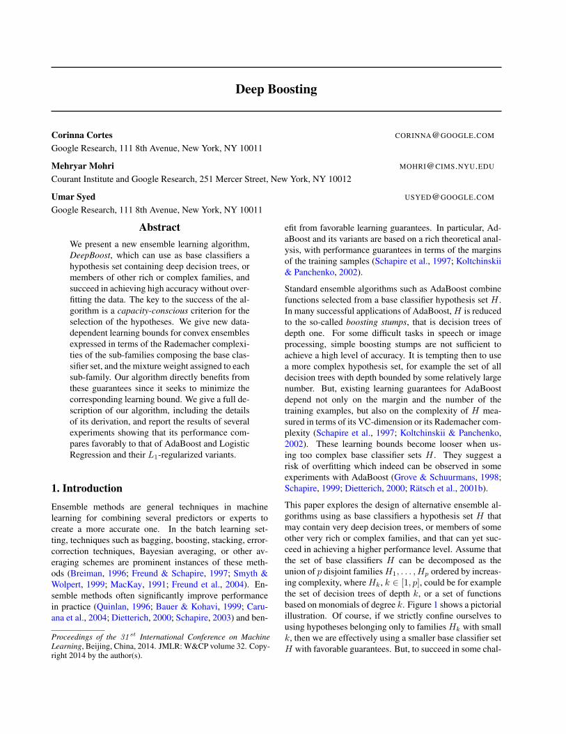
This paper explores the design of alternative ensemble al-gorithms using as base classifiers a hypothesis set H thatmay contain very deep decision trees, or members of someother very rich or complex families, and that can yet suc-ceed in achieving a higher performance level. Assume thatthe set of base classifiers H can be decomposed as theunion of p disjoint families H

1

, . . . ,Hp ordered by increas-ing complexity, where Hk, k 2 [1, p], could be for examplethe set of decision trees of depth k, or a set of functionsbased on monomials of degree k. Figure 1 shows a pictorialillustration. Of course, if we strictly confine ourselves tousing hypotheses belonging only to families Hk with smallk, then we are effectively using a smaller base classifier setH with favorable guarantees. But, to succeed in some chal-

Deep Boosting

H1

H2

H3

H4

H5

H1

H1

[H2

· · ·H

1

[· · · [Hp

Figure 1. Base classifier set H decomposed in terms of sub-families H1, . . . , Hp or their unions.

lenging tasks, the use of a few more complex hypothesescould be needed. The main idea behind the design of ouralgorithms is that an ensemble based on hypotheses drawnfrom H

1

, . . . ,Hp can achieve a higher accuracy by makinguse of hypotheses drawn from Hks with large k if it allo-cates more weights to hypotheses drawn from Hks with asmall k. But, can we determine quantitatively the amountsof mixture weights apportioned to different families? Canwe provide learning guarantees for such algorithms?

Note that our objective is somewhat reminiscent of that ofmodel selection, in particular Structural Risk Minimization(SRM) (Vapnik, 1998), but it differs from that in that wedo not wish to limit our base classifier set to some optimalHq =

Sqk=1

Hk. Rather, we seek the freedom of using asbase hypotheses even relatively deep trees from rich Hks,with the promise of doing so infrequently, or that of re-serving them a somewhat small weight contribution. Thisprovides the flexibility of learning with deep hypotheses.

We present a new algorithm, DeepBoost, whose design isprecisely guided by the ideas just discussed. Our algorithmis grounded in a solid theoretical analysis that we presentin Section 2. We give new data-dependent learning boundsfor convex ensembles. These guarantees are expressed interms of the Rademacher complexities of the sub-familiesHk and the mixture weight assigned to each Hk, in ad-dition to the familiar margin terms and sample size. Ourcapacity-conscious algorithm is derived via the applicationof a coordinate descent technique seeking to minimize suchlearning bounds. We give a full description of our algo-rithm, including the details of its derivation and its pseu-docode (Section 3) and discuss its connection with previ-ous boosting-style algorithms. We also report the results ofseveral experiments (Section 4) demonstrating that its per-formance compares favorably to that of AdaBoost, whichis known to be one of the most competitive binary classifi-cation algorithms.

2. Data-dependent learning guarantees forconvex ensembles with multiple hypothesissets

Non-negative linear combination ensembles such as boost-ing or bagging typically assume that base functions are se-lected from the same hypothesis set H . Margin-based gen-eralization bounds were given for ensembles of base func-tions taking values in {�1,+1} by Schapire et al. (1997) in

terms of the VC-dimension of H . Tighter margin boundswith simpler proofs were later given by Koltchinskii &Panchenko (2002), see also (Bartlett & Mendelson, 2002),for the more general case of a family H taking arbitraryreal values, in terms of the Rademacher complexity of H .

Here, we also consider base hypotheses taking arbitraryreal values but assume that they can be selected from sev-eral distinct hypothesis sets H

1

, . . . ,Hp with p � 1 andpresent margin-based learning in terms of the Rademachercomplexity of these sets. Remarkably, the complexity termof these bounds admits an explicit dependency in terms ofthe mixture coefficients defining the ensembles. Thus, theensemble family we consider is F = conv(

Spk=1

Hk), thatis the family of functions f of the form f =

PTt=1

↵tht,where ↵ = (↵

1

, . . . ,↵T ) is in the simplex � and where,for each t 2 [1, T ], ht is in Hkt for some kt 2 [1, p].

Let X denote the input space. H1

, . . . ,Hp are thus fam-ilies of functions mapping from X to R. We considerthe familiar supervised learning scenario and assume thattraining and test points are drawn i.i.d. according to somedistribution D over X ⇥ {�1,+1} and denote by S =

((x1

, y1

), . . . , (xm, ym)) a training sample of size m drawnaccording to Dm.

Let ⇢ > 0. For a function f taking values in R, we de-note by R(f) its binary classification error, by R⇢(f) its⇢-margin error, and by bRS,⇢(f) its empirical margin error:

R(f) = E

(x,y)⇠D[1yf(x)0

], R⇢(f) = E

(x,y)⇠D[1yf(x)⇢],

bR⇢(f) = E

(x,y)⇠S[1yf(x)⇢],

where the notation (x, y) ⇠ S indicates that (x, y) is drawnaccording to the empirical distribution defined by S.

The following theorem gives a margin-based Rademachercomplexity bound for learning with such functions in thebinary classification case. As with other Rademacher com-plexity learning guarantees, our bound is data-dependent,which is an important and favorable characteristic of ourresults. For p = 1, that is for the special case of a singlehypothesis set, the analysis coincides with that of the stan-dard ensemble margin bounds (Koltchinskii & Panchenko,2002).Theorem 1. Assume p > 1. Fix ⇢ > 0. Then, for any� > 0, with probability at least 1 � � over the choice ofa sample S of size m drawn i.i.d. according to Dm, thefollowing inequality holds for all f =

PTt=1

↵tht 2 F:

R(f) bRS,⇢(f) +

4

⇢

TX

t=1

↵tRm(Hkt)

+

2

⇢

rlog p

m+

s⇠4

⇢2

log

h ⇢2m

log p

i⇡log p

m+

log

2

�

2m.

Deep Boosting

Thus, R(f) bRS,⇢(f) +

4

⇢

PTt=1

↵tRm(Hkt) + C(m, p)

with C(m, p) = O⇣q

log p⇢2m log

⇥⇢2mlog p

⇤⌘.

This result is remarkable since the complexity term in theright-hand side of the bound admits an explicit depen-dency on the mixture coefficients ↵t. It is a weighted aver-age of Rademacher complexities with mixture weights ↵t,t 2 [1, T ]. Thus, the second term of the bound suggeststhat, while some hypothesis sets Hk used for learning couldhave a large Rademacher complexity, this may not be detri-mental to generalization if the corresponding total mixtureweight (sum of ↵ts corresponding to that hypothesis set) isrelatively small. Such complex families offer the potentialof achieving a better margin on the training sample.

The theorem cannot be proven via a standard Rademachercomplexity analysis such as that of Koltchinskii &Panchenko (2002) since the complexity term of the boundwould then be the Rademacher complexity of the familyof hypotheses F = conv(

Spk=1

Hk) and would not de-pend on the specific weights ↵t defining a given func-tion f . Furthermore, the complexity term of a standardRademacher complexity analysis is always lower boundedby the complexity term appearing in our bound. Indeed,since Rm(conv([p

k=1

Hk)) = Rm([pk=1

Hk), the follow-ing lower bound holds for any choice of the non-negativemixtures weights ↵t summing to one:

Rm(F) � mmax

k=1

Rm(Hk) �TX

t=1

↵tRm(Hkt). (1)

Thus, Theorem 1 provides a finer learning bound than theone obtained via a standard Rademacher complexity anal-ysis. The full proof of the theorem is given in Appendix A.Our proof technique exploits standard tools used to de-rive Rademacher complexity learning bounds (Koltchin-skii & Panchenko, 2002) as well as a technique used bySchapire, Freund, Bartlett, and Lee (1997) to derive earlyVC-dimension margin bounds. Using other standard tech-niques as in (Koltchinskii & Panchenko, 2002; Mohri et al.,2012), Theorem 1 can be straightforwardly generalized tohold uniformly for all ⇢ > 0 at the price of an additional

term that is in O⇣q

log log

2⇢

m

⌘.

3. AlgorithmIn this section, we will use the learning guarantees of Sec-tion 2 to derive a capacity-conscious ensemble algorithmfor binary classification.

3.1. Optimization problem

Let H1

, . . . ,Hp be p disjoint families of functions takingvalues in [�1,+1] with increasing Rademacher complex-

ities Rm(Hk), k 2 [1, p]. We will assume that the hy-pothesis sets Hk are symmetric, that is, for any h 2 Hk,we also have (�h) 2 Hk, which holds for most hypothe-sis sets typically considered in practice. This assumptionis not necessary but it helps simplifying the presentation ofour algorithm. For any hypothesis h 2 [p

k=1

Hk, we denoteby d(h) the index of the hypothesis set it belongs to, that ish 2 Hd(h)

. The bound of Theorem 1 holds uniformly forall ⇢ > 0 and functions f 2 conv(

Spk=1

Hk).1 Since thelast term of the bound does not depend on ↵, it suggestsselecting ↵ to minimize

G(↵) =

1

m

mX

i=1

1yiPT

t=1 ↵tht(xi)⇢ +

4

⇢

TX

t=1

↵trt,

where rt = Rm(Hd(ht)). Since for any ⇢ > 0, f and f/⇢

admit the same generalization error, we can instead searchfor ↵ � 0 with

PTt=1

↵t 1/⇢ which leads to

min

↵�0

1

m

mX

i=1

1yiPT

t=1↵tht(xi)1

+4

TX

t=1

↵trt s.t.TX

t=1

↵t 1

⇢.

The first term of the objective is not a convex functionof ↵ and its minimization is known to be computation-ally hard. Thus, we will consider instead a convex upperbound. Let u 7! �(�u) be a non-increasing convex func-tion upper bounding u 7! 1u0

with � differentiable overR and �

0(u) 6= 0 for all u. � may be selected to be for

example the exponential function as in AdaBoost (Freund& Schapire, 1997) or the logistic function. Using such anupper bound, we obtain the following convex optimizationproblem:

min

↵�0

1

m

mX

i=1

�

⇣1� yi

TX

t=1

↵tht(xi)

⌘+ �

TX

t=1

↵trt (2)

s.t.TX

t=1

↵t 1

⇢,

where we introduced a parameter � � 0 controlling the bal-ance between the magnitude of the values taken by function� and the second term. Introducing a Lagrange variable� � 0 associated to the constraint in (2), the problem canbe equivalently written as

min

↵�0

1

m

mX

i=1

�

⇣1� yi

TX

t=1

↵tht(xi)

⌘+

TX

t=1

(�rt + �)↵t.

Here, � is a parameter that can be freely selected by thealgorithm since any choice of its value is equivalent to a

1The conditionPT

t=1 ↵t = 1 of Theorem 1 can be relaxedto

PTt=1 ↵t 1. To see this, use for example a null hypothesis

(ht = 0 for some t).

Deep Boosting

choice of ⇢ in (2). Let {h1

, . . . , hN} be the set of distinctbase functions, and let G be the objective function basedon that collection:

G(↵)=

1

m

mX

i=1

�

⇣1�yi

NX

j=1

↵jhj(xi)

⌘+

NX

t=1

(�rj +�)↵j ,

with ↵ = (↵1

, . . . ,↵N ) 2 RN . Note that we can drop therequirement ↵ � 0 since the hypothesis sets are symmetricand ↵tht = (�↵t)(�ht). For each hypothesis h, we keepeither h or �h in {h

1

, . . . , hN}. Using the notation

⇤j = �rj + �, (3)

for all j 2 [1, N ], our optimization problem can then berewritten as min↵ F (↵) with

F (↵)=

1

m

mX

i=1

�

⇣1�yi

NX

j=1

↵jhj(xi)

⌘+

NX

t=1

⇤j |↵j |, (4)

with no non-negativity constraint on ↵. The function Fis convex as a sum of convex functions and admits a sub-differential at all ↵ 2 R. We can design a boosting-stylealgorithm by applying coordinate descent to F (↵).

Let ↵t = (↵t,1, . . . ,↵t,N )

> denote the vector obtained af-ter t � 1 iterations and let ↵

0

= 0. Let ek denote thekth unit vector in RN , k 2 [1, N ]. The direction ek andthe step ⌘ selected at the tth round are those minimizingF (↵t�1

+ ⌘ek), that is

F (↵t�1

+ ⌘ek)=

1

m

mX

i=1

�

⇣1� yift�1

(xi)�⌘yihk(xi)

⌘

+

X

j 6=k

⇤j |↵t�1,j |+ ⇤k|↵t�1,k + ⌘|,

where ft�1

=

PNj=1

↵t�1,jhj . For any t 2 [1, T ], wedenote by Dt the distribution defined by

Dt(i) =

�

0�1� yift�1

(xi)�

St, (5)

where St is a normalization factor, St =

Pmi=1

�

0(1 �

yift�1

(xi)). For any s 2 [1, T ] and j 2 [1, N ], we denoteby ✏s,j the weighted error of hypothesis hj for the distribu-tion Ds, for s 2 [1, T ]:

✏s,j =

1

2

h1� E

i⇠Ds

[yihj(xi)]

i. (6)

3.2. DeepBoost

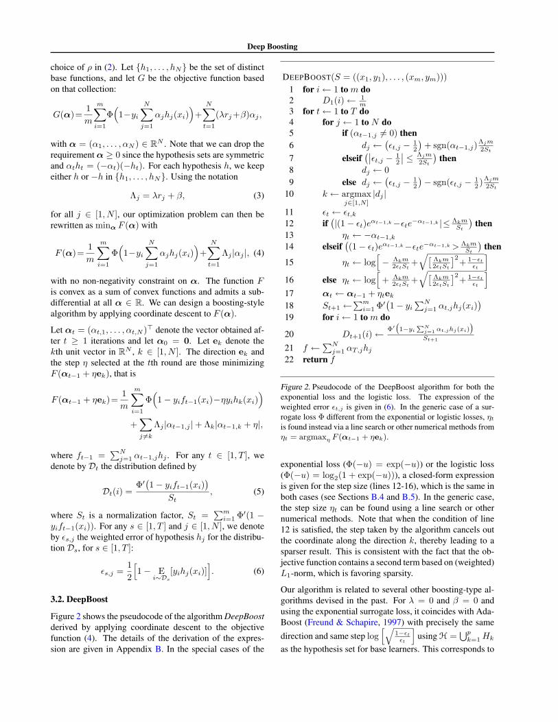
Figure 2 shows the pseudocode of the algorithm DeepBoostderived by applying coordinate descent to the objectivefunction (4). The details of the derivation of the expres-sion are given in Appendix B. In the special cases of the

DEEPBOOST(S = ((x1

, y1

), . . . , (xm, ym)))

1 for i 1 to m do2 D

1

(i) 1

m3 for t 1 to T do4 for j 1 to N do5 if (↵t�1,j 6= 0) then6 dj

�✏t,j � 1

2

�+ sgn(↵t�1,j)

⇤jm2St

7 elseif��✏t,j � 1

2

�� ⇤jm2St

�then

8 dj 0

9 else dj �✏t,j � 1

2

�� sgn(✏t,j � 1

2

)

⇤jm2St

10 k argmax

j2[1,N ]

|dj |

11 ✏t ✏t,k

12 if�|(1� ✏t)e↵t�1,k�✏te�↵t�1,k | ⇤km

St

�then

13 ⌘t �↵t�1,k

14 elseif�(1� ✏t)e↵t�1,k�✏te�↵t�1,k > ⇤km

St

�then

15 ⌘t log

h� ⇤km

2✏tSt+

q⇥⇤km2✏tSt

⇤2

+

1�✏t

✏t

i

16 else ⌘t log

h+

⇤km2✏tSt

+

q⇥⇤km2✏tSt

⇤2

+

1�✏t

✏t

i

17 ↵t ↵t�1

+ ⌘tek

18 St+1

Pm

i=1

�

0�1� yi

PNj=1

↵t,jhj(xi)�

19 for i 1 to m do

20 Dt+1

(i) �

0�1�yi

PNj=1 ↵t,jhj(xi)

�

St+1

21 f PN

j=1

↵T,jhj

22 return f

Figure 2. Pseudocode of the DeepBoost algorithm for both theexponential loss and the logistic loss. The expression of theweighted error ✏t,j is given in (6). In the generic case of a sur-rogate loss � different from the exponential or logistic losses, ⌘t

is found instead via a line search or other numerical methods from⌘t = argmax⌘ F (↵t�1 + ⌘ek).

exponential loss (�(�u) = exp(�u)) or the logistic loss(�(�u) = log

2

(1 + exp(�u))), a closed-form expressionis given for the step size (lines 12-16), which is the same inboth cases (see Sections B.4 and B.5). In the generic case,the step size ⌘t can be found using a line search or othernumerical methods. Note that when the condition of line12 is satisfied, the step taken by the algorithm cancels outthe coordinate along the direction k, thereby leading to asparser result. This is consistent with the fact that the ob-jective function contains a second term based on (weighted)L

1

-norm, which is favoring sparsity.

Our algorithm is related to several other boosting-type al-gorithms devised in the past. For � = 0 and � = 0 andusing the exponential surrogate loss, it coincides with Ada-Boost (Freund & Schapire, 1997) with precisely the samedirection and same step log

hq1�✏t

✏t

iusing H =

Spk=1

Hk

as the hypothesis set for base learners. This corresponds to

Deep Boosting

ignoring the complexity term of our bound as well as thecontrol of the sum of the mixture weights via �. For � = 0

and � = 0 and using the logistic surrogate loss, our algo-rithm also coincides with additive logistic loss (Friedmanet al., 1998).

In the special case where � = 0 and � 6= 0 and forthe exponential surrogate loss, our algorithm matches theL

1

-norm regularized AdaBoost (e.g., see (Ratsch et al.,2001a)). For the same choice of the parameters and forthe logistic surrogate loss, our algorithm matches the L

1

-norm regularized additive Logistic Regression studied byDuchi & Singer (2009) using the base learner hypothesisset H =

Spk=1

Hk. H may in general be very rich. The keyfoundation of our algorithm and analysis is instead to takeinto account the relative complexity of the sub-families Hk.Also, note that L

1

-norm regularized AdaBoost and Logis-tic Regression can be viewed as algorithms minimizing thelearning bound obtained via the standard Rademacher com-plexity analysis (Koltchinskii & Panchenko, 2002), usingthe exponential or logistic surrogate losses. Instead, theobjective function minimized by our algorithm is based onthe generalization bound of Theorem 1, which as discussedearlier is a finer bound (see (1)). For � = 0 but � 6= 0, ouralgorithm is also close to the so-called unnormalized Arc-ing (Breiman, 1999) or AdaBoost⇢ (Ratsch & Warmuth,2002) using H as a hypothesis set. AdaBoost⇢ coincideswith AdaBoost modulo the step size, which is more con-servative than that of AdaBoost and depends on ⇢. Ratsch& Warmuth (2005) give another variant of the algorithmthat does not require knowing the best ⇢, see also the re-lated work of Kivinen & Warmuth (1999); Warmuth et al.(2006).

Our algorithm directly benefits from the learning guaran-tees given in Section 2 since it seeks to minimize the boundof Theorem 1. In the next section, we report the results ofour experiments with DeepBoost. Let us mention that wehave also designed an alternative deep boosting algorithmthat we briefly describe and discuss in Appendix C.

4. ExperimentsAn additional benefit of the learning bounds presented inSection 2 is that they are data-dependent. They are basedon the Rademacher complexity of the base hypothesis setsHk, which in some cases can be well estimated from thetraining sample. The algorithm DeepBoost directly inher-its this advantage. For example, if the hypothesis set Hk

is based on a positive definite kernel with sample matrixKk, it is known that its empirical Rademacher complexity

can be upper bounded byp

Tr[Kk]

m and lower bounded by1p2

pTr[Kk]

m . In other cases, when Hk is a family of func-tions taking binary values, we can use an upper bound on

the Rademacher complexity in terms of the growth func-

tion of Hk, ⇧Hk(m): Rm(Hk)

q2 log ⇧Hk

(m)

m . Thus,for the family Hstumps

1

of boosting stumps in dimension d,⇧Hstumps

1(m) 2md, since there are 2m distinct threshold

functions for each dimension with m points. Thus, the fol-lowing inequality holds:

Rm(Hstumps1

) r

2 log(2md)

m. (7)

Similarly, we consider the family of decision trees Hstumps2

of depth 2 with the same question at the internal nodes ofdepth 1. We have ⇧Hstumps

2(m) (2m)

2

d(d�1)

2

since thereare d(d � 1)/2 distinct trees of this type and since eachinduces at most (2m)

2 labelings. Thus, we can write

Rm(Hstumps2

) r

2 log(2m2d(d� 1))

m. (8)

More generally, we also consider the family of all binarydecision trees H trees

k of depth k. For this family it is knownthat VC-dim(H trees

k ) (2

k+ 1) log

2

(d + 1) (Mansour,1997). More generally, the VC-dimension of Tn, the fam-ily of decision trees with n nodes in dimension d can bebounded by (2n + 1) log

2

(d + 2) (see for example (Mohri

et al., 2012)). Since Rm(H) q

2 VC-dim(H) log(m+1)

m ,for any hypothesis class H we have

Rm(Tn) r

(4n + 2) log

2

(d + 2) log(m + 1)

m. (9)

The experiments with DeepBoost described below use ei-ther Hstumps

= Hstumps1

[Hstumps2

or HtreesK =

SKk=1

H treesk ,

for some K > 0, as the base hypothesis sets. For any hy-pothesis in these sets, DeepBoost will use the upper boundsgiven above as a proxy for the Rademacher complexityof the set to which it belongs. We leave it to the futureto experiment with finer data-dependent estimates or up-per bounds on the Rademacher complexity, which couldfurther improve the performance of our algorithm. Re-call that each iteration of DeepBoost searches for the basehypothesis that is optimal with respect to a certain crite-rion (see lines 5-10 of Figure 2). While an exhaustivesearch is feasible for Hstumps

1

, it would be far too expen-sive to visit all trees in Htrees

K when K is large. There-fore, when using Htrees

K and also Hstumps2

as the base hy-potheses we use the following heuristic search procedurein each iteration t: First, the optimal tree h⇤

1

2 H trees1

isfound via exhaustive search. Next, for all 1 < k K,a locally optimal tree h⇤k 2 H trees

k is found by consider-ing only trees that can be obtained by adding a single layerof leaves to h⇤k�1

. Finally, we select the best hypothesesin the set {h⇤

1

, . . . , h⇤K , h1

, . . . , ht�1

}, where h1

, . . . , ht�1

are the hypotheses selected in previous iterations.

Deep Boosting

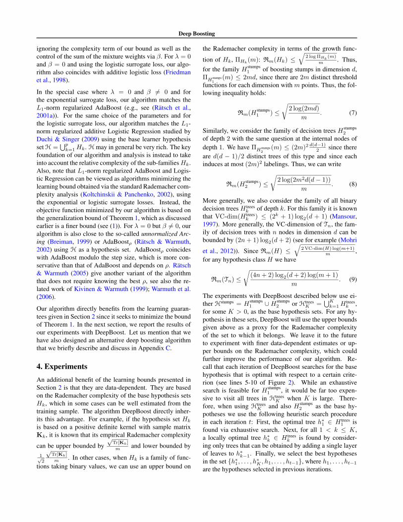
Table 1. Results for boosted decision stumps and the exponential loss function.

AdaBoost AdaBoost AdaBoost AdaBoostbreastcancer Hstumps

1 Hstumps2 AdaBoost-L1 DeepBoost ocr17 Hstumps

1 Hstumps2 AdaBoost-L1 DeepBoost

Error 0.0429 0.0437 0.0408 0.0373 Error 0.0085 0.008 0.0075 0.0070(std dev) (0.0248) (0.0214) (0.0223) (0.0225) (std dev) 0.0072 0.0054 0.0068 (0.0048)

Avg tree size 1 2 1.436 1.215 Avg tree size 1 2 1.086 1.369Avg no. of trees 100 100 43.6 21.6 Avg no. of trees 100 100 37.8 36.9

AdaBoost AdaBoost AdaBoost AdaBoostionosphere Hstumps

1 Hstumps2 AdaBoost-L1 DeepBoost ocr49 Hstumps



Avg tree size 1 2 1.392 1.168 Avg tree size 1 2 1.99 1.96Avg no. of trees 100 100 39.35 17.45 Avg no. of trees 100 100 99.3 96

AdaBoost AdaBoost AdaBoost AdaBoostgerman Hstumps

1 Hstumps2 AdaBoost-L1 DeepBoost ocr17-mnist Hstumps



Avg tree size 1 2 1.54 1.76 Avg tree size 1 2 2 1.99Avg no. of trees 100 100 54.1 76.5 Avg no. of trees 100 100 100 100

AdaBoost AdaBoost AdaBoost AdaBoostdiabetes Hstumps

1 Hstumps2 AdaBoost-L1 DeepBoost ocr49-mnist Hstumps



Avg tree size 1 2 1.9975 1.9975 Avg tree size 1 2 1.9975 1.9975Avg no. of trees 100 100 100 100 Avg no. of trees 100 100 100 100

Breiman (1999) and Reyzin & Schapire (2006) extensivelyinvestigated the relationship between the complexity of de-cision trees in an ensemble learned by AdaBoost and thegeneralization error of the ensemble. We tested DeepBooston the same UCI datasets used by these authors, http://archive.ics.uci.edu/ml/datasets.html, specifi-cally breastcancer, ionosphere, german(numeric)and diabetes. We also experimented with two opticalcharacter recognition datasets used by Reyzin & Schapire(2006), ocr17 and ocr49, which contain the handwrittendigits 1 and 7, and 4 and 9 (respectively). Finally, becausethese OCR datasets are fairly small, we also constructedthe analogous datasets from all of MNIST, http://yann.lecun.com/exdb/mnist/, which we call ocr17-mnistand ocr49-mnist. More details on all the datasets aregiven in Table 4, Appendix D.1.

As we discussed in Section 3.2, by fixing the parameters �and � to certain values, we recover some known algorithmsas special cases of DeepBoost. Our experiments comparedDeepBoost to AdaBoost (� = � = 0 with exponentialloss), to Logistic Regression (� = � = 0 with logisticloss), which we abbreviate as LogReg, to L

1

-norm regular-ized AdaBoost (e.g., see (Ratsch et al., 2001a)) abbreviatedas AdaBoost-L1, and also to the L

1

-norm regularized ad-ditive Logistic Regression algorithm studied by (Duchi &Singer, 2009) (� > 0,� = 0) abbreviated as LogReg-L1.

In the first set of experiments reported in Table 1, we com-pared AdaBoost, AdaBoost-L1, and DeepBoost with theexponential loss (�(�u) = exp(�u)) and base hypothe-ses Hstumps. We tested standard AdaBoost with base hy-potheses Hstumps

1

and Hstumps2

. For AdaBoost-L1, we op-

timized over � 2 {2�i: i = 6, . . . , 0} and for Deep-

Boost, we optimized over � in the same range and � 2{0.0001, 0.005, 0.01, 0.05, 0.1, 0.5}. The exact parameteroptimization procedure is described below.

In the second set of experiments reported in Table 2, weused base hypotheses Htrees

K instead of Hstumps, where themaximum tree depth K was an additional parameter to beoptimized. Specifically, for AdaBoost we optimized overK 2 {1, . . . , 6}, for AdaBoost-L1 we optimized over thosesame values for K and � 2 {10

�i: i = 3, . . . , 7}, and for

DeepBoost we optimized over those same values for K, �and � 2 {10

�i: i = 3, . . . , 7}.

The last set of experiments, reported in Table 3, are identi-cal to the experiments reported in Table 2, except we usedthe logistic loss �(�u) = log

2

(1 + exp(�u)).

We used the following parameter optimization procedurein all experiments: Each dataset was randomly partitionedinto 10 folds, and each algorithm was run 10 times, with adifferent assignment of folds to the training set, validationset and test set for each run. Specifically, for each run i 2{0, . . . , 9}, fold i was used for testing, fold i + 1 (mod 10)

was used for validation, and the remaining folds were usedfor training. For each run, we selected the parameters thathad the lowest error on the validation set and then measuredthe error of those parameters on the test set. The averageerror and the standard deviation of the error over all 10 runsis reported in Tables 1, 2 and 3, as is the average number oftrees and the average size of the trees in the ensembles.

In all of our experiments, the number of iterations was setto 100. We also experimented with running each algorithm

http://archive.ics.uci.edu/ml/datasets.html

http://archive.ics.uci.edu/ml/datasets.html

http://yann.lecun.com/exdb/mnist/

http://yann.lecun.com/exdb/mnist/

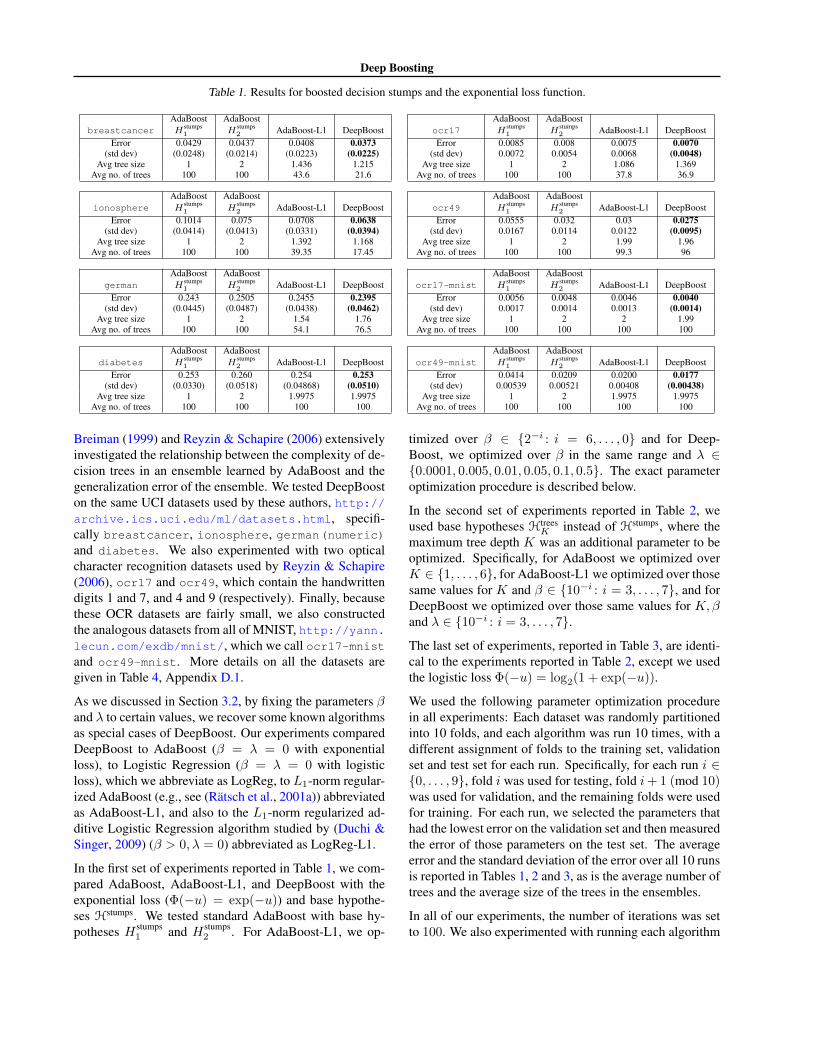
Deep Boosting

Table 2. Results for boosted decision trees and the exponential loss function.

breastcancer AdaBoost AdaBoost-L1 DeepBoost ocr17 AdaBoost AdaBoost-L1 DeepBoostError 0.0267 0.0264 0.0243 Error 0.004 0.003 0.002

(std dev) (0.00841) (0.0098) (0.00797) (std dev) (0.00316) (0.00100) (0.00100)Avg tree size 29.1 28.9 20.9 Avg tree size 15.0 30.4 26.0

Avg no. of trees 67.1 51.7 55.9 Avg no. of trees 88.3 65.3 61.8

ionosphere AdaBoost AdaBoost-L1 DeepBoost ocr49 AdaBoost AdaBoost-L1 DeepBoostError 0.0661 0.0657 0.0501 Error 0.0180 0.0175 0.0175

(std dev) (0.0315) (0.0257) (0.0316) (std dev) (0.00555) (0.00357) (0.00510)Avg tree size 29.8 31.4 26.1 Avg tree size 30.9 62.1 30.2


german AdaBoost AdaBoost-L1 DeepBoost ocr17-mnist AdaBoost AdaBoost-L1 DeepBoostError 0.239 0.239 0.234 Error 0.00471 0.00471 0.00409

(std dev) (0.0165) (0.0201) (0.0148) (std dev) (0.0022) (0.0021) (0.0021)Avg tree size 3 7 16.0 Avg tree size 15 33.4 22.1


diabetes AdaBoost AdaBoost-L1 DeepBoost ocr49-mnist AdaBoost AdaBoost-L1 DeepBoostError 0.249 0.240 0.230 Error 0.0198 0.0197 0.0182

(std dev) (0.0272) (0.0313) (0.0399) (std dev) (0.00500) (0.00512) (0.00551)Avg tree size 3 3 5.37 Avg tree size 29.9 66.3 30.1


Table 3. Results for boosted decision trees and the logistic loss function.

breastcancer LogReg LogReg-L1 DeepBoost ocr17 LogReg LogReg-L1 DeepBoostError 0.0351 0.0264 0.0264 Error 0.00300 0.00400 0.00250

(std dev) (0.0101) (0.0120) (0.00876) (std dev) (0.00100) (0.00141) (0.000866)Avg tree size 15 59.9 14.0 Avg tree size 15.0 7 22.1


ionosphere LogReg LogReg-L1 DeepBoost ocr49 LogReg LogReg-L1 DeepBoostError 0.074 0.060 0.043 Error 0.0205 0.0200 0.0170

(std dev) (0.0236) (0.0219) (0.0188) (std dev) (0.00654) (0.00245) (0.00361)Avg tree size 7 30.0 18.4 Avg tree size 31.0 31.0 63.2


german LogReg LogReg-L1 DeepBoost ocr17-mnist LogReg LogReg-L1 DeepBoostError 0.233 0.232 0.225 Error 0.00422 0.00417 0.00399

(std dev) (0.0114) (0.0123) (0.0103) (std dev) (0.00191) (0.00188) (0.00211)Avg tree size 7 7 14.4 Avg tree size 15 15 25.9


diabetes LogReg LogReg-L1 DeepBoost ocr49-mnist LogReg LogReg-L1 DeepBoostError 0.250 0.246 0.246 Error 0.0211 0.0201 0.0201

(std dev) (0.0374) (0.0356) (0.0356) (std dev) (0.00412) (0.00433) (0.00411)Avg tree size 3 3 3 Avg tree size 28.7 33.5 72.8


for up to 1,000 iterations, but observed that the test errorsdid not change significantly, and more importantly the or-dering of the algorithms by their test errors was unchangedfrom 100 iterations to 1,000 iterations.

Observe that with the exponential loss, DeepBoost has asmaller test error than AdaBoost and AdaBoost-L1 on ev-ery dataset and for every set of base hypotheses, except forthe ocr49-mnist dataset with decision trees where its per-formance matches that of AdaBoost-L1. Similarly, with thelogistic loss, DeepBoost performs always at least as well asLogReg or LogReg-L1. For the small-sized UCI datasets itis difficult to obtain statistically significant results, but, forthe larger ocrXX-mnist datasets, our results with Deep-Boost are statistically significantly better at the 2% levelusing one-sided paired t-tests in all three sets of experi-ments (three tables), except for ocr49-mnist in Table 3,

where this holds only for the comparison with LogReg.

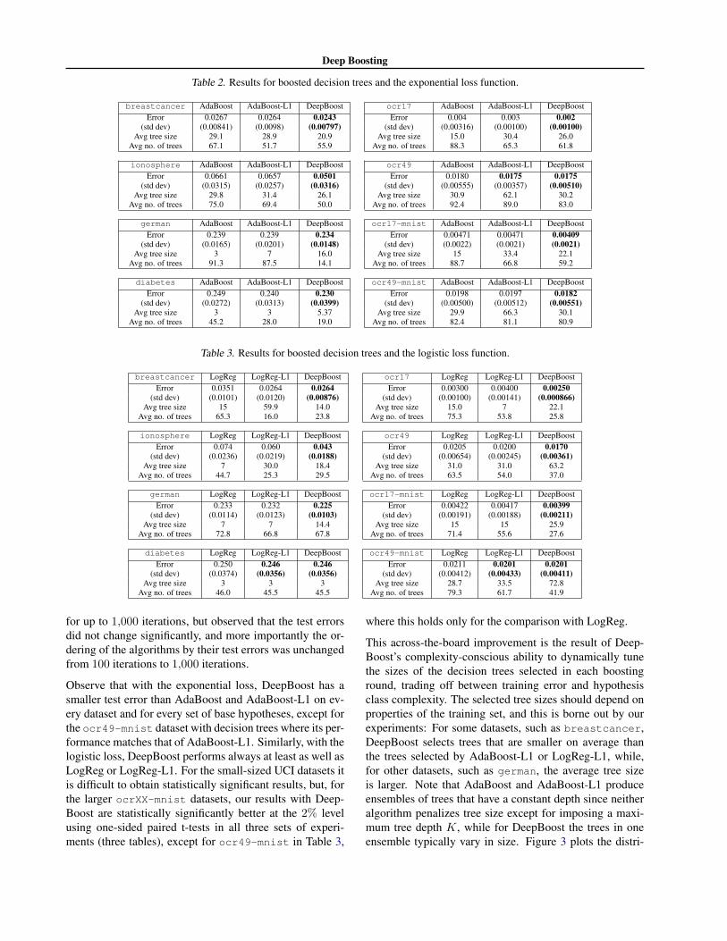
This across-the-board improvement is the result of Deep-Boost’s complexity-conscious ability to dynamically tunethe sizes of the decision trees selected in each boostinground, trading off between training error and hypothesisclass complexity. The selected tree sizes should depend onproperties of the training set, and this is borne out by ourexperiments: For some datasets, such as breastcancer,DeepBoost selects trees that are smaller on average thanthe trees selected by AdaBoost-L1 or LogReg-L1, while,for other datasets, such as german, the average tree sizeis larger. Note that AdaBoost and AdaBoost-L1 produceensembles of trees that have a constant depth since neitheralgorithm penalizes tree size except for imposing a maxi-mum tree depth K, while for DeepBoost the trees in oneensemble typically vary in size. Figure 3 plots the distri-

Deep Boosting

Ion: Histogram of tree sizes

Tree sizes

Frequency

10 20 30 40

024681012

Figure 3. Distribution of tree sizes when DeepBoost is run on theionosphere dataset.

bution of tree sizes for one run of DeepBoost. It shouldbe noted that the columns for AdaBoost in Table 1 simplylist the number of stumps to be the same as the number ofboosting rounds; a careful examination of the ensemblesfor 100 rounds of boosting typically reveals a 5% duplica-tion of stumps in the ensembles.

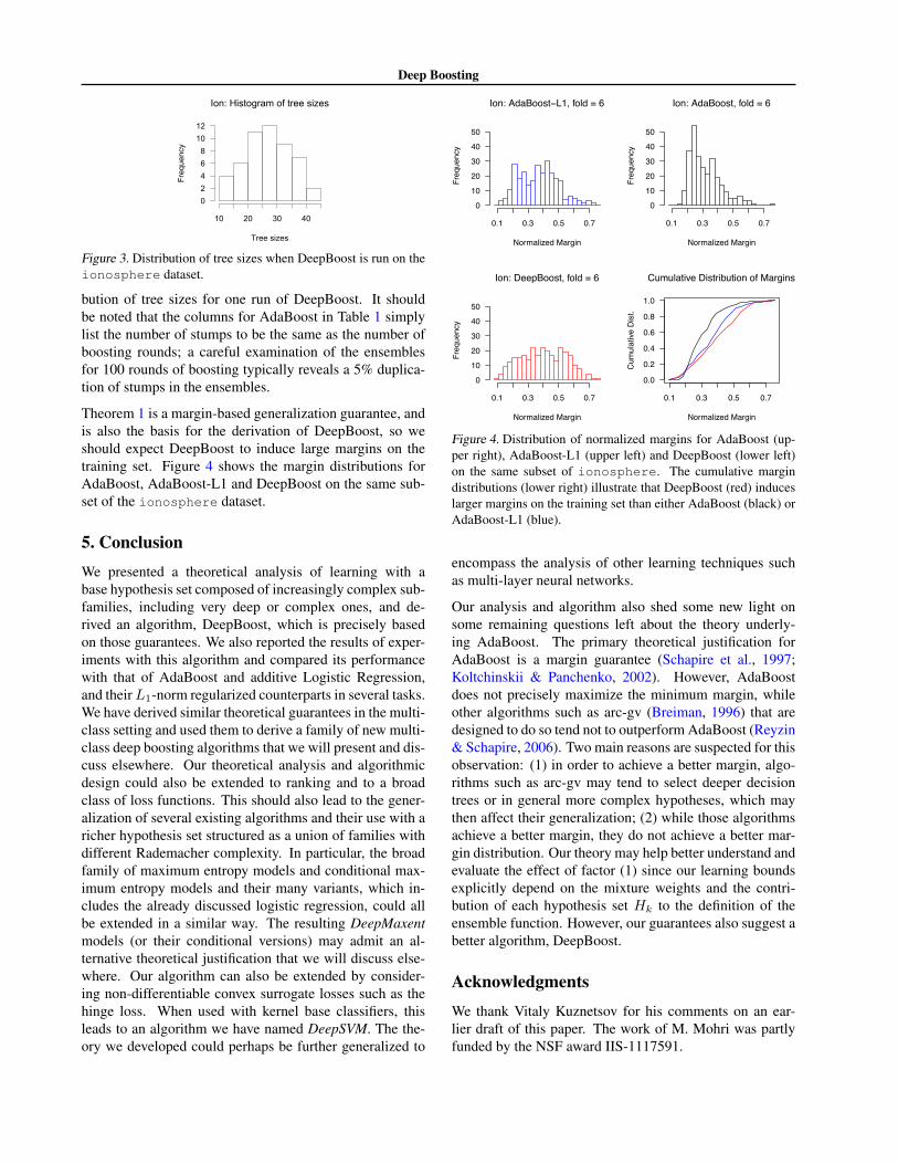
Theorem 1 is a margin-based generalization guarantee, andis also the basis for the derivation of DeepBoost, so weshould expect DeepBoost to induce large margins on thetraining set. Figure 4 shows the margin distributions forAdaBoost, AdaBoost-L1 and DeepBoost on the same sub-set of the ionosphere dataset.

5. ConclusionWe presented a theoretical analysis of learning with abase hypothesis set composed of increasingly complex sub-families, including very deep or complex ones, and de-rived an algorithm, DeepBoost, which is precisely basedon those guarantees. We also reported the results of exper-iments with this algorithm and compared its performancewith that of AdaBoost and additive Logistic Regression,and their L

1

-norm regularized counterparts in several tasks.We have derived similar theoretical guarantees in the multi-class setting and used them to derive a family of new multi-class deep boosting algorithms that we will present and dis-cuss elsewhere. Our theoretical analysis and algorithmicdesign could also be extended to ranking and to a broadclass of loss functions. This should also lead to the gener-alization of several existing algorithms and their use with aricher hypothesis set structured as a union of families withdifferent Rademacher complexity. In particular, the broadfamily of maximum entropy models and conditional max-imum entropy models and their many variants, which in-cludes the already discussed logistic regression, could allbe extended in a similar way. The resulting DeepMaxentmodels (or their conditional versions) may admit an al-ternative theoretical justification that we will discuss else-where. Our algorithm can also be extended by consider-ing non-differentiable convex surrogate losses such as thehinge loss. When used with kernel base classifiers, thisleads to an algorithm we have named DeepSVM. The the-ory we developed could perhaps be further generalized to

Ion: AdaBoost−L1, fold = 6

Normalized Margin

Freq

uenc

y

0.1 0.3 0.5 0.7

01020304050

Ion: AdaBoost, fold = 6

Normalized Margin

Freq

uenc

y

0.1 0.3 0.5 0.7

01020304050

Ion: DeepBoost, fold = 6

Normalized Margin

Freq

uenc

y

0.1 0.3 0.5 0.7

01020304050

0.1 0.3 0.5 0.7

0.0

0.2

0.4

0.6

0.8

1.0

Normalized Margin

Cum

ulat

ive D

ist.

Cumulative Distribution of Margins

Figure 4. Distribution of normalized margins for AdaBoost (up-per right), AdaBoost-L1 (upper left) and DeepBoost (lower left)on the same subset of ionosphere. The cumulative margindistributions (lower right) illustrate that DeepBoost (red) induceslarger margins on the training set than either AdaBoost (black) orAdaBoost-L1 (blue).

encompass the analysis of other learning techniques suchas multi-layer neural networks.

Our analysis and algorithm also shed some new light onsome remaining questions left about the theory underly-ing AdaBoost. The primary theoretical justification forAdaBoost is a margin guarantee (Schapire et al., 1997;Koltchinskii & Panchenko, 2002). However, AdaBoostdoes not precisely maximize the minimum margin, whileother algorithms such as arc-gv (Breiman, 1996) that aredesigned to do so tend not to outperform AdaBoost (Reyzin& Schapire, 2006). Two main reasons are suspected for thisobservation: (1) in order to achieve a better margin, algo-rithms such as arc-gv may tend to select deeper decisiontrees or in general more complex hypotheses, which maythen affect their generalization; (2) while those algorithmsachieve a better margin, they do not achieve a better mar-gin distribution. Our theory may help better understand andevaluate the effect of factor (1) since our learning boundsexplicitly depend on the mixture weights and the contri-bution of each hypothesis set Hk to the definition of theensemble function. However, our guarantees also suggest abetter algorithm, DeepBoost.

AcknowledgmentsWe thank Vitaly Kuznetsov for his comments on an ear-lier draft of this paper. The work of M. Mohri was partlyfunded by the NSF award IIS-1117591.

Deep Boosting

ReferencesBartlett, Peter L. and Mendelson, Shahar. Rademacher and

Gaussian complexities: Risk bounds and structural re-sults. JMLR, 3, 2002.

Bauer, Eric and Kohavi, Ron. An empirical comparison ofvoting classification algorithms: Bagging, boosting, andvariants. Machine Learning, 36(1-2):105–139, 1999.

Breiman, Leo. Bagging predictors. Machine Learning, 24(2):123–140, 1996.

Breiman, Leo. Prediction games and arcing algorithms.Neural Computation, 11(7):1493–1517, 1999.

Caruana, Rich, Niculescu-Mizil, Alexandru, Crew, Geoff,and Ksikes, Alex. Ensemble selection from libraries ofmodels. In ICML, 2004.

Dietterich, Thomas G. An experimental comparison ofthree methods for constructing ensembles of decisiontrees: Bagging, boosting, and randomization. MachineLearning, 40(2):139–157, 2000.

Duchi, John C. and Singer, Yoram. Boosting with structuralsparsity. In ICML, pp. 38, 2009.

Freund, Yoav and Schapire, Robert E. A decision-theoreticgeneralization of on-line learning and an application toboosting. Journal of Computer System Sciences, 55(1):119–139, 1997.

Freund, Yoav, Mansour, Yishay, and Schapire, Robert E.Generalization bounds for averaged classifiers. The An-nals of Statistics, 32:1698–1722, 2004.

Friedman, Jerome, Hastie, Trevor, and Tibshirani, Robert.Additive logistic regression: a statistical view of boost-ing. Annals of Statistics, 28:2000, 1998.

Grove, Adam J and Schuurmans, Dale. Boosting in thelimit: Maximizing the margin of learned ensembles. InAAAI/IAAI, pp. 692–699, 1998.

Kivinen, Jyrki and Warmuth, Manfred K. Boosting as en-tropy projection. In COLT, pp. 134–144, 1999.

Koltchinskii, Vladmir and Panchenko, Dmitry. Empiri-cal margin distributions and bounding the generalizationerror of combined classifiers. Annals of Statistics, 30,2002.

MacKay, David J. C. Bayesian methods for adaptive mod-els. PhD thesis, California Institute of Technology, 1991.

Mansour, Yishay. Pessimistic decision tree pruning basedon tree size. In Proceedings of ICML, pp. 195–201,1997.

Mohri, Mehryar, Rostamizadeh, Afshin, and Talwalkar,Ameet. Foundations of Machine Learning. The MITPress, 2012.

Quinlan, J. Ross. Bagging, boosting, and C4.5. InAAAI/IAAI, Vol. 1, pp. 725–730, 1996.

Ratsch, Gunnar and Warmuth, Manfred K. Maximizing themargin with boosting. In COLT, pp. 334–350, 2002.

Ratsch, Gunnar and Warmuth, Manfred K. Efficient marginmaximizing with boosting. Journal of Machine LearningResearch, 6:2131–2152, 2005.

Ratsch, Gunnar, Mika, Sebastian, and Warmuth, Man-fred K. On the convergence of leveraging. In NIPS, pp.487–494, 2001a.

Ratsch, Gunnar, Onoda, Takashi, and Muller, Klaus-Robert. Soft margins for AdaBoost. Machine Learning,42(3):287–320, 2001b.

Reyzin, Lev and Schapire, Robert E. How boosting themargin can also boost classifier complexity. In ICML,pp. 753–760, 2006.

Schapire, Robert E. Theoretical views of boosting and ap-plications. In Proceedings of ALT 1999, volume 1720 ofLecture Notes in Computer Science, pp. 13–25. Springer,1999.

Schapire, Robert E. The boosting approach to machinelearning: An overview. In Nonlinear Estimation andClassification, pp. 149–172. Springer, 2003.

Schapire, Robert E., Freund, Yoav, Bartlett, Peter, and Lee,Wee Sun. Boosting the margin: A new explanation forthe effectiveness of voting methods. In ICML, pp. 322–330, 1997.

Smyth, Padhraic and Wolpert, David. Linearly combiningdensity estimators via stacking. Machine Learning, 36:59–83, July 1999.

Vapnik, Vladimir N. Statistical Learning Theory. Wiley-Interscience, 1998.

Warmuth, Manfred K., Liao, Jun, and Ratsch, Gunnar. To-tally corrective boosting algorithms that maximize themargin. In ICML, pp. 1001–1008, 2006.

deep boosting - proceedings of machine learning researchproceedings.mlr.press/v32/cortesb14.pdf ·...

Documents