a new mathematical approach to geographic profiling new mathematical approach to geographic...

The author(s) shown below used Federal funds provided by the U.S. Department of Justice and prepared the following final report:

Document Title: A New Mathematical Approach to Geographic Profiling

Author: Mike O’Leary Document No.: 237985

Date Received: March 2012 Award Number: 2007-DE-BX-K005

This report has not been published by the U.S. Department of Justice. To provide better customer service, NCJRS has made this Federally-funded grant final report available electronically in addition to traditional paper copies.

Opinions or points of view expressed are those of the author(s) and do not necessarily reflect

the official position or policies of the U.S. Department of Justice.

A New Mathematical Approach to Geographic Profiling

Mike O’LearyDepartment of Mathematics

Towson University

December 14, 2009

This document is a research report submitted to the U.S. Department of Justice. This report has not been published by the Department. Opinions or points of view expressed are those of the author(s) and do not necessarily reflect the official position or policies of the U.S. Department of Justice.

Abstract

The primary question in geographic profiling is, given the locations of a series of crimes committedby the same serial offender, to estimate the location of that offender’s anchor point. Currently, thereare three main approaches to the problem, exemplified by the three software systems- CrimeStat,Dragnet, and Rigel. Though the details of the approaches taken by these software packages differ,they share a common mathematical heritage.

In our work, we developed an fundamentally new mathematical framework for the geographicprofiling problem. Our framework meets our five essential goals:

1. The framework is mathematically rigorous;

2. There are explicit connections between assumptions on offender behavior and the compo-nents of the mathematical model;

3. The framework takes into account local geographic features; in particular it accounts for

(a) Geographic features that influence the selection of a crime site, and

(b) Geographic features that influence the potential anchor points of offenders;

4. The framework is based exclusively on data that is local to the jurisdiction(s) where theoffenses occur; and

5. The framework returns a prioritized search area for law enforcement officers.

Our mathematical approach to this problem is based on Bayesian inference, and begins withthe explicit ansatz that the offender’s choice of targets depends only on (1) the distance betweenthe target and the offender’s anchor point, and (2) local geographic features of the target location.The algorithm requires a representative list of historical crimes of the same type as the series; thisis used to estimate the local target attractiveness. The algorithm uses an estimate of the prior distri-bution of offender anchor points taken from local population density. The algorithm also estimatesthe structure of the offender’s distance decay behavior; as a prior it takes a list of solved crimestogether with the corresponding anchor point. With the model and appropriate priors selected, themathematical framework then used Bayesian methods to develop an estimate for the probabilitydistribution of the offender’s anchor point based on the locations of the crime series.

This mathematical model has been implemented in software. Our tool is broken down into twopackages. The first is a graphical user interface that lets the analyst or officer enter the requireddata, and comes complete with help features, and a set of instructions. The second tool performsthe actual mathematical analysis; because it is separate from the user interface, it could potentiallybe used as a component in other tools.

The software tool is freely available for download, and is now currently being tested by both theBaltimore County Police Department as well as the Los Angeles Police Department. The sourcecode for both tools are available, together with extensive documentation.


Contents

1 Executive Summary 3

2 Introduction 82.1 Statement of the problem . . . . . . . . . . . . . . . . . . . . . . . . . . . . . . . 82.2 Literature . . . . . . . . . . . . . . . . . . . . . . . . . . . . . . . . . . . . . . . 102.3 Statement of hypothesis . . . . . . . . . . . . . . . . . . . . . . . . . . . . . . . . 14

3 Methods 163.1 The mathematical model . . . . . . . . . . . . . . . . . . . . . . . . . . . . . . . 16

3.1.1 Bayesian Analysis . . . . . . . . . . . . . . . . . . . . . . . . . . . . . . 173.1.2 Simple Models for Offender Behavior . . . . . . . . . . . . . . . . . . . . 193.1.3 More Realistic Models for Offender Behavior . . . . . . . . . . . . . . . . 203.1.4 Future Offense Prediction . . . . . . . . . . . . . . . . . . . . . . . . . . 23

3.2 Implementing the mathematical model . . . . . . . . . . . . . . . . . . . . . . . . 243.2.1 Measuring distance . . . . . . . . . . . . . . . . . . . . . . . . . . . . . . 253.2.2 The distance decay . . . . . . . . . . . . . . . . . . . . . . . . . . . . . . 253.2.3 Estimating the prior distribution of average offense distances . . . . . . . . 28

Tikhonov regularization . . . . . . . . . . . . . . . . . . . . . . . . . . . 303.2.4 The geographic triangulation . . . . . . . . . . . . . . . . . . . . . . . . . 41

The coarse mesh . . . . . . . . . . . . . . . . . . . . . . . . . . . . . . . 41Finding the orientation of the coarse mesh’s triangles . . . . . . . . 43Finding the centroids of the coarse mesh’s triangles . . . . . . . . . 44Determining the coarse mesh triangle containing a point . . . . . . 46Determining the coarse mesh triangle near a point . . . . . . . . . . 46

The fine mesh . . . . . . . . . . . . . . . . . . . . . . . . . . . . . . . . . 49Triangular coordinates . . . . . . . . . . . . . . . . . . . . . . . . 49Subtriangles with the same orientation as the parent . . . . . . . . . 49Subtriangles with the opposite orientation as the parent . . . . . . . 51Cartesian Coordinates . . . . . . . . . . . . . . . . . . . . . . . . 51

3.2.5 Evaluating the probability densityP (z) . . . . . . . . . . . . . . . . . . . 533.2.6 The Normalization Function . . . . . . . . . . . . . . . . . . . . . . . . . 53

The Tail . . . . . . . . . . . . . . . . . . . . . . . . . . . . . . . . . . . . 54The discretization . . . . . . . . . . . . . . . . . . . . . . . . . . . . . . . 55

The two-dimensional midpoint rule . . . . . . . . . . . . . . . . . 55Application to the normalization function . . . . . . . . . . . . . . 57

1


Selecting the mesh . . . . . . . . . . . . . . . . . . . . . . . . . . . . . . 57EvaluatingI(z, α) asz varies . . . . . . . . . . . . . . . . . . . . . . . . 57EvaluatingI(z, α) asα varies . . . . . . . . . . . . . . . . . . . . . . . . 59

3.3 Reprise of mathematical assumptions and computational techniques . . . . . . . . 613.4 The software . . . . . . . . . . . . . . . . . . . . . . . . . . . . . . . . . . . . . 62

3.4.1 Overview . . . . . . . . . . . . . . . . . . . . . . . . . . . . . . . . . . . 623.4.2 Installing the software . . . . . . . . . . . . . . . . . . . . . . . . . . . . 643.4.3 Using the software . . . . . . . . . . . . . . . . . . . . . . . . . . . . . . 64

Selecting the crime series . . . . . . . . . . . . . . . . . . . . . . . . . . . 64Selecting the historical crime locations . . . . . . . . . . . . . . . . . . . 64Selecting the historical distances . . . . . . . . . . . . . . . . . . . . . . . 66Selecting the search region . . . . . . . . . . . . . . . . . . . . . . . . . . 66Selecting the offender information . . . . . . . . . . . . . . . . . . . . . . 67Program results . . . . . . . . . . . . . . . . . . . . . . . . . . . . . . . . 67The analysis . . . . . . . . . . . . . . . . . . . . . . . . . . . . . . . . . 67Running time . . . . . . . . . . . . . . . . . . . . . . . . . . . . . . . . . 68

3.4.4 Internal structure of the software . . . . . . . . . . . . . . . . . . . . . . . 68Profiler . . . . . . . . . . . . . . . . . . . . . . . . . . . . . . . . . . . . 68

Using Profiler as a stand-alone program . . . . . . . . . . . . . . . 68Compiling Profiler . . . . . . . . . . . . . . . . . . . . . . . . . . 71Brief overview of the Profiler source code . . . . . . . . . . . . . . 71

ProfilerGUI . . . . . . . . . . . . . . . . . . . . . . . . . . . . . . . . . . 75Compiling ProfilerGUI . . . . . . . . . . . . . . . . . . . . . . . . 75Brief overview of the ProfilerGUI source code . . . . . . . . . . . 75Integrating Profiler and ProfilerGUI . . . . . . . . . . . . . . . . . 76

4 Results 774.1 Discussion of findings . . . . . . . . . . . . . . . . . . . . . . . . . . . . . . . . . 774.2 Implications for policy and practice . . . . . . . . . . . . . . . . . . . . . . . . . 844.3 Implications for further research . . . . . . . . . . . . . . . . . . . . . . . . . . . 84

Bibliography 86

Dissemination of Research Findings 92

List of Supplemental Material 92

2


Chapter 1

Executive Summary

The primary question in geographic profiling is, given the locations of a series of crimes committedby the same serial offender, to estimate the location of that offender’s anchor point. Currently, thereare three main approaches to the problem, exemplified by the three software systems- CrimeStat,Dragnet, and Rigel. Though the details of the approaches taken by these software packages differ,they share a common mathematical heritage.

In our work, we developed an fundamentally new mathematical framework for the geographicprofiling problem and implemented in prototype software that is now freely available for down-load1. Both our mathematical approach and our software tool are able to account for geographicfeatures that affect the selection of the crime sites, geographic features that affect the distributionof potential anchor points, differences in the travel distances of different offenders, and certaindemographic characteristics (race/ethnic group, age, and sex) of the offender.

To begin our discussion of our mathematical model, let us agree to adopt some common nota-tion. A pointx will have two componentsx = (x(1), x(2)). These can be latitude and longitude,or distances from a fixed pair of perpendicular reference axes. We presume that we are workingwith a series ofn linked crimes, and the crime sites under consideration are labeledx1,x2, . . . ,xn.We use the symbolz to denote the offender’s anchor point. The anchor point can be the offender’shome, place of work, or some other location of importance to the offender.

We begin by assuming that our offender chooses potential locations to offend randomly ac-cording to some unknown probability density functionP (x). The use of a probability distributionhere is not meant to indicate that the offender is choosing targets randomly, though that may be thecase. Instead it represents our lack of knowledge of the decision making process of the offender.

We assume thatP depends on just two factors; first is the anchor pointz of the offender. Secondis the average distance that our offender is willing to travel to offend. We know that differentoffenders have a different willingness to travel and that the travel patterns of a fifteen year old willbe different that those of a forty year old. For that reason we explicitly allow for the possibilitythat the offender’s average travel distance may affect the choice of targets by the offender.

Thus, our initial mathematical model is that the offender with anchor pointz and averageoffense distanceα chooses to offend at the locationx according to an unknown probability distri-butionP (x | z, α). The elements of the crime seriesx1,x2, . . . ,xn then represent a sample fromthis unknown distribution.

1http://pages.towson.edu/moleary/Profiler.html

3


http://pages.towson.edu/moleary/Profiler.html

Now we suppose that we specify the form ofP (x | z, α); then the geographic profiling problembecomes a parameter identification problem for the unknown parametersz andα. We approachthis problem using Bayesian methods to try to find a probability distribution for the unknownparameters. Standard Bayesian theory tells us that the posterior distribution ofz andα given aseries of crimesx1,x2, . . . ,xn is

P (z, α |x1,x2, . . . ,xn) =P (x1,x2, . . . ,xn | z, α)π(z, α)

P (x1,x2, . . . ,xn).

HereP (x1,x2, . . . ,xn | z, α) is our model of offender behavior; it specifies the probability densitythat the offender will offend at all of the locationsx1,x2, . . . ,xn given that they have anchor pointz and average offense distanceα. The factorπ(z, α) is the prior distribution of anchor point andoffense distance; it represents what we know about the offender before we take into account theinformation from the crime series itself. The factorP (x1,x2, . . . ,xn) is the marginal distribution;since it does not depend on eitherz or α, we can remove it provided we replace the equality by aproportionality, so

P (z, α |x1,x2, . . . ,xn) ∝ P (x1,x2, . . . ,xn | z, α)π(z, α).

We next assume that the different crime sites were chosen independently of one another. Thischoice is made because it is the simplest way we can relate the distributionP (x1,x2, . . . ,xn | z, α)to our model of offender behaviorP (x | z, α). However, there is some evidence that criminaloffense sites are not independent, which would require a more sophisticated model for offenderbehavior. Proceeding with the simplest model of independence though, we can then say that

P (x1,x2, . . . ,xn | z, α) = P (x1 | z, α)P (x2 | z, α) . . . P (xn | z, α).

The simplest approach to the priorπ(z, α) is to assume that anchor points and offense distancesare independent; then we can write

π(z, α) = H(z)π(α).

HereH(z) represents our knowledge of the distribution of offender anchor points before we in-corporate information about the crime series. We take the approach that the distribution of anchorpoints can be modeled by population density; areas with high population density will correspondto areas with high anchor point density. We can then calculateH(z) by simply using U.S. Censusdata; moreover because U.S. Census data is sorted by sex, age, and race / ethnic group all theway to the block level, we can incorporate these demographic factors whenH(z) is calculated. Inpractice, we calculateH(z) from the Census data by using a kernel density parameter estimationtechnique

H(z) =

Nblocks∑

i=1

= piK(z − qi |√

Ai)

where each block has populationpi, centerqi and for each block we have chosen a differentbandwidth equal to the side length of a square with the same areaAi as the block. HereK(x | λ)is a truncated quartic kernel with bandwidthλ, so that

K(x|λ) =

3

πλ6(|x|2 − λ2)2 if |x| ≤ λ,

0 if |x| ≥ λ.

4


The prior distribution of offender average offense distanceπ(α) is more difficult to estimate.Indeed, though distribution of distances are available across offenses from aggregated historicaldata, we need to obtain the distribution of average offense distances across offenders. However,we are able to link the historical aggregate data with the behavior of individual offenders througha Fredholm integral equation, whose solution can then be estimated. This process is entirely au-tomated within our software tool, and the user simply needs to obtain a list of historical solvedcrimes of the same general type as the crime series.

Combining these, we then see that we have the relationship

P (z, α |x1,x2, . . . ,xn) ∝ P (x1 | z, α)P (x2 | z, α) . . . P (xn | z, α)H(z)π(α)

and since we are only interested in the distribution of the anchor points, we take the conditionaldistribution to obtain

P (z |x1,x2, . . . ,xn) ∝∫ ∞

0

P (x1 | z, α)P (x2 | z, α) . . . P (xn | z, α)H(z)π(α) dα

which gives the probability distribution that the offender has anchor pointz, given that they havecommitted crimes atx1,x2, . . . ,xn.

For this approach to be useful though, we still need to specify a model for offender behaviorP (x | z, α). We take the approach that this has the form

P (x | z, α) = D(d(x, z), α)G(x)N(z, α).

Here the factorD(d(x, z), α) accounts for the distance decay behavior of the offender. The termd(x, z) is the distance between the pointsx andz. The mathematical framework does not force anyparticular choice of the distance metric on us, however since our software uses latitude and longi-tude internally to represent points, we use a spherical distance metric. Similarly, the mathematicalframework does not force any particular form for the distance decay term. Our software uses aRayleigh distribution; this was chosen because this is the distribution of distances that results froma bivariate normal distribution, and bivariate normal distributions appear naturally as the limit ofrandom walks. Thus, we use the factor

D(d, α) =πd

2α2exp

(

−πd2

4α2

)

.

The factorG(x) is present because some crimes can only occur at certain pre-defined locations,such as liquor store robberies or bank robberies. Even if the crime type is not limited to certainlocations, it is still more likely to occur in some regions than others, like street robberies. This fac-tor lets us account for these variations. It represents the local target attractiveness of a location, sothat areas whereG(x) are considered to be more likely locations of an offense that regions whereG(x) is small. Rather than try to determine somea priori form for G(x) based on criminologicalmodels, we instead simply assume that past behavior is a reasonable predictor of future behav-ior. In particular, to calculateG(x), we start with a list of historical crimesc1, c2, . . . , cN . Wethen construct the local target attractiveness function using a kernel density parameter estimationtechnique by calculating

G(x) =

N∑

i=1

K(x − ci | λ)

5


where the bandwidthλ is twice the mean nearest neighbor distance between historical crime sites.This is essentially the same as one of the methods used to generate crime hot spots.

The last factor,N(z, α) is a normalization factor, which ensures thatP actually represents aprobability distribution. It is determined by our choice ofD andG, and has the form

N(z, α) =1

∫∫

D(d(y, z), α)G(y)dy(1)dy(2).

This completes the specification of our mathematical framework, and shows us how we canestimate the location of the anchor point of an offender using as data:

• The locations of the crime series,

• The locations of historically similar crimes, to generate our estimate forG(x),

• A list of solved historical crimes, with both the locations of the offense site and the corre-sponding anchor point, to generate our estimate ofπ(α), and

• Census data, along with any available demographic information about the offender, this letsus estimateH(z).

This mathematical approach meets our five essential goals:








Once the mathematical development was complete, we needed to turn these ideas into a prac-tical tool that could be useful to law enforcement. To that end, we have developed software thatimplements these mathematical algorithms. The software was built in two parts:

• A program called Profiler that performs all of the mathematical analysis, and

• A program called ProfilerGUI with which the user interacts.

An analyst who wishes to use our algorithm need only download the software package and runProfilerGUI. That program provides a convenient user interface that allows the user to enter all ofthe data necessary for the analysis in a simple form; it then calls the Profiler program to actuallyperform the analysis. When finished, it provides the user with a map of the proposed search area

6


in .kml format; is also provides the analyst with a map of the target attractiveness functionG(x),as well as a map of the local population densityH(z).

Because the software was built in two components, others who wish to incorporate the mathe-matical analysis tools of Profiler are able to do so.

This project has resulted in two main implications for policy and practice. First by providinga new tool for the geographic profiling problem to police agencies, we hope to directly improvethe clearance rate for series crimes.We presented our first functional prototype software packageat the NIJ Conference in June 2009. The program is now being used by both the Los AngelesPolice Department and the Baltimore County Police Department, both of whom are examining theeffectiveness and usefulness of the tool.

It should be noted however, that we have not yet made a study of the effectiveness of the toolor of the mathematical algorithms that it contains.

On the other hand, by making our mathematics, algorithms and code widely and publicly avail-able, we also hope that we can provide valuable insights to other researchers.

7


Chapter 2

Introduction

2.1 Statement of the problem

The purpose of our project was to develop and implement improved mathematical methods forthe geographic profiling problem. Geographic profiling is a technique to used to make predictionsabout the location of a serial offender’s anchor point or home base, based on the known locationsof that offender’s offenses. Prior to this work, three main software suites existed for geographicprofiling. They are CrimeStat- developed by Ned Levine, Dragnet- developed by David Canter,and Rigel- developed by Kim Rossmo. These three software suites share a common mathematicalheritage, and use mathematically related methods to determine their estimates of the offender’sanchor point.

In our work, we developed an fundamentally new mathematical framework for the geographicprofiling problem. Our framework meets our five essential goals:








Ensuring that the mathematical algorithms are rigorous and making explicit the connectionsbetween the assumptions on offender behavior and components of the model helps in the analysisof the model. In particular, it gives researchers another tool to evaluate a model; one issue withthe current generation of software suites for geographic profiling is that there is little agreementbetween the principals on how to compare the effectiveness of these differing approaches.

8


It is important that the mathematics explicitly allows for the influence of the local geographyand demography. It is well known that there are relationships between the physical environmentand crime rates; see for example Brantingham and Brantingham [8]. It is essential that a goodmathematical framework possess the ability to incorporate this information into the model. Thatsaid, it is equally important that the model uses only data that is available to the appropriate lawenforcement agency. Even if we were somehow able to create the perfect algorithm that alwayscorrectly predicts an offender’s anchor point, that algorithm would still be worthless if it requireddata unavailable to law enforcement.

Finally, we recognize that simple point estimates of offender anchor points are not very valuableto practicing law enforcement officers. Rather, to be useful to practitioners, the algorithm mustproduce prioritized search areas.

There is clearly a need for improvement in geographic profiling. Indeed, the National Instituteof Justice’s Mapping Analysis and Public Safety web site1 says

“Though there have been anecdotal successes with geographic profiling, there havealso been several instances where geographic profiling has either been wrong on pre-dicting where the offender lives/works or has been inappropriate as a model. Thusfar, none of the geographic profiling software packages have been subject to rigorous,independent or comparative tests to evaluate their accuracy, reliability, validity, utility,or appropriateness for various situations.”

Some of the issues that face existing algorithms may be due to their common mathematicalheritage. Indeed, it may be the case that the limiting feature of these existing algorithms actuallylies in the mathematics upon which they are based. Clearly, no approach to geographic profilingcan be more accurate than their underlying algorithm will let them be.

In our work we have developed a fundamentally new and rigorous mathematical technique thatestimates the location of an offender’s anchor point.

Our approach is to start with the assumption that an offender has a single stable anchor point.We then assume that the offender chooses crime locations according to a probability density func-tion with two factors: first is a distance decay from the offender’s anchor point, while the secondis a local target attractiveness.

We make noa priori mathematical restrictions on the choice and form of the distance decaycomponent. The mathematics allows for the use of the Euclidean, Manhattan, or any other distancemetric; the form of the distance decay function can have any of the common mathematical forms-normal, negative exponential, or experimentally determined.

The local target density is determined by direct calculation from historical data. For example,if an analyst is examining a series of late night street robberies, then the algorithm requires arepresentative sample of historical late night street robberies. From this information, we estimatethe likelihood that this particular crime occurs at any given location. This mathematical analysisproceeds under the assumption that the historical information is a reasonable predictor of currentcrime rates.

Given both the distance decay functional form, and the local target density, we obtain a familyof probability density functions, one for each potential anchor point for the offender. We could thenuse maximum likelihood methods to estimate the anchor point of the offender [14]. However, this

1http://www.ojp.usdoj.gov/nij/maps/gp.htm , accessed August 2009

9


http://www.ojp.usdoj.gov/nij/maps/gp.htm

approach only provides a point estimate for the location of the offender’s anchor point. Instead, weapply Bayesian techniques to estimate the probability distribution for the offender’s anchor point,and so provide a map of the regions that are more or less likely to contain the offender’s anchorpoint.

We have created and developed the mathematics necessary for this analysis, and implementedthe resulting algorithms in software. The tool we have developed has now been released, and isbeing tested by both the Baltimore County Police Department and the Los Angeles Police Depart-ment.

2.2 Literature

To begin our review of the current state of geographic profiling, let us agree to adopt some commonnotation. A pointx will have two componentsx = (x(1), x(2)). These can be latitude and longitude,or distances from a fixed pair of perpendicular reference axes. We presume that we are workingwith a series ofn linked crimes, and the crime sites under consideration are labeledx1,x2, . . . ,xn.We use the symbolz to denote the offender’s anchor point. The anchor point can be the offender’shome, place of work, or some other location of importance to the offender.

An important first question in geographic profiling is how to measure the distance betweenpoints. One common method is to use the usual notion of distance, called the Euclidean distance.In this case, the distanced(x,y) between two pointsx andy is given byd2(x,y) where

d2(x,y) =√

[x(1) − y(1)]2 + [x(2) − y(2)]2

Another approach is to use the Manhattan distance; in this case the distance betweenx andy isgiven byd1(x,y) where

d1(x,y) = |x(1) − y(1)| + |x(2) − y(2)|There are other choices that can be used as well; for example the total street distance following thelocal road network, or the total time to make the trip while following the local road network.

One important difference to note between these distances is that the Euclidean distance givesthe same results regardless of the choice of the coordinate axes; in particular, rotating a pair ofpoints around a third does not change the distance between the pair. This result does not hold forthe Manhattan distance, and so the coordinate axes need to be chosen with care when using theManhattan distance.

Following Snook, Zito, Bennell and Taylor [52], we classify algorithms for geographic profil-ing into two general categories- spatial distribution strategies and probability distance strategies.

Spatial distribution strategies. The simplest of the spatial distribution strategies is to estimatethe offenders anchor pointz by the centroidζcentroid of the crime series [27]. The centroid, alsoknown as the center of mass is defined to be

ζcentroid =1

n

n∑

i=1

xi.

Another approach is to estimate the anchor pointz by the center of minimum distanceζcmd.This is chosen to be the value ofy for which the sum of the distances from the point to the crime

10


sites

D(y) =n∑

i=1

d(xi,y)

is a minimum. Here different choices of the distance functiond lead to different choices for thecenter of minimum distance. Unlike the centroid, there is no simple formula that gives the valueof ζcmd; however, there are a number of efficient algorithms that can approximate it to any desiredaccuracy.

Another method used to estimate the anchor point is the circle method of Canter and Larkin[12]. They make a distinction between two types of offenders; marauders and commuters. Amarauder is assumed to move from a home base, commit a crime, and then return, where the baseacts as a focal point for the crime series. In this case, the offender’s home range and criminalrange overlap. A commuter, on the other hand, first moves from a home base to another area, thencommits the crime. As a consequence, the focal point for the crime series is different from thehome base, and the offender’s home range and criminal range do not overlap

Their circle hypothesis is the following. Given a series of linked crimes committed by a ma-rauder, draw a circle whose diameter are the two crimes locations that are the farthest apart. Thenall of the crimes in the series would be in the resulting circle, and the offender’s home base wouldalso lie in the circle so drawn.

There is evidence for the validity of the circle hypothesis. In their original paper, Canter andLarkin [12] examined a collection of 45 male sexual assaults in Britain. In 41 of the 45 cases thecircle correctly encompassed all of the crime sites and in 39 of the 45 cases the circle correctlycontained a base for the offender. Kocsis and Irwin [22] examined 24 rape series, 22 arson series,and 27 burglary series in Australia. The circle contained all of the crimes for 79% of the rapeseries, 82% of the arson series, and 70% of the burglary series, while the circle correctly containedthe home base of the offender for 71% of the rape cases, 82% of the arson cases, and 48% ofthe burglary cases. This last result suggests that the marauder hypotheses may not necessarily beappropriate for burglary.

These results were amplified by Meany [35], who showed that burglars were more likely toact as commuters than non-burglars, while arsonists and sex offenders were more likely to act asmarauders than non-arsonists / non-sex offenders. Similarly, Kocsis, Cooksey, Irwin and Allen[21] found in their study of 58 burglaries that occurred in rural Australian towns, that the circletheory was less effective. Laukkanen and Santtila [25] examined 76 commercial robbery series,and found only 30 (=39%) that satisfied the circle hypothesis. Note however, that many of theseseries were very short; 62 of the 76 series analyzed contained either two or three crimes.

Probability distribution strategiesIn contrast to the spatial distribution strategies are the prob-ability distance strategies. These methods are currently employed in the major computer programsfor geographic profiling (CrimeStat, Dragnet, and Rigel). All have the common idea of construct-ing a hit score by summing the values of some decay function of the distances between a generalpoint and the elements of the crime series. Mathematically, they all begin by first making a choiceof distance metricd; they then select a decay functionf and construct a hit score functionS(y) bycomputing

S(y) =n∑

i=1

f(d(xi,y)) = f(d(x1,y)) + · · ·+ f(d(xn,y)). (2.1)

Regions with a high hit score are considered to be more likely to contain the offender’s anchor

11


point than regions with a low hit score. In practice, the hit scoreS(y) is not evaluated everywhere,but simply on some rectangular array of pointsyjk = (y

(1)j , y

(2)k ) for j ∈ {1, 2, . . . J} andk ∈

{1, 2, . . . , K}, giving us the array of valuesSjk = S(yjk).In effect, these approaches center a tent function on each of the crime sites; the hit score is

then found by summing the results. The differences between the different methods are solely inthe choice of the tent function.

Rossmo’s method, as described in [41, Chapter 10] chooses the Manhattan distance functionfor d and the decay function

f(d) =

k

dhif d < B,

kBg−h

(2B − d)gif d ≥ B.

We remark that Rossmo also considers the possibility of forming hit scores by multiplication; see[41, p. 200]

The method described by Canter, Coffey, Huntley and Missen in [11] is to use a Euclideandistance, and to choose either a decay function in the form

f(d) = e−βd

or functions with a buffer and plateau, with the form

f(d) =

0 if d < A,

B if A ≤ d < B,

Ce−βd if d ≥ B.

The CrimeStat program described in [29] uses Euclidean or spherical distance and gives theuser a number of choices for the decay function, including

• Linear:f(d) = A + Bd,

• Negative exponential:f(d) = Ae−βd,

• Normal:f(d) = A(2πS2)−1/2 exp [−(d − d)2/2S2],

• Lognormal:f(d) = A(2πd2S2)−1/2 exp [−(ln d − d)2/2S2], and

• Truncated negative exponential:f(d) = Bd if d < C andf(d) = Ae−βd if d ≥ C.

CrimeStat also allows the user to use empirical data to create a different decay function matchinga set of provided data as well as the use of indirect distances.

Though each of these approaches are distinct, they share the same underlying mathematicalstructure; they vary only in the choice of decay function and the choice of distance metric.

Bayesian methodsWe remark that the latest version (3.2) of CrimeStat contains a new BayesianJourney to Crime Module that integrates information on the origin location of other offenders whocommitted crimes in the same location with the distance decay estimates [30]. In this approach,the geographic region under consideration is subdivided into subregionsRi; then the matrixCij

12


is formed, which counts the number of crimes that occur in region Ri committed by an offenderwith anchor point inRj. This is then used as the prior distribution for the Bayesian analysis. Inparticular if a series of crimes is concentrated in regionRi, then by examining the matrixCij,regionsRj for whichCij is large are considered to be more likely to contain the offender’s anchorpoint than regions whereCij is small. Levine and Block [31]have tested this method with datafrom Baltimore County and from Chicago.

Controversies. There is some question as to whether or not computer GIS systems imple-menting the existing algorithms are as effective as simply providing humans with some simpleheuristics;c.f. the discussion in Snook, Canter, and Bennell [48], Snook, Taylor and Bennell [49],Rossmo [43] and Snook, Taylor and Bennell [51]; see also the discussion in Snook, Taylor andBennell [50], Rossmo and Filer [44], Bennell, Snook and Taylor [4] and Rossmo, Filey and Sesley[45]; see also the paper of Bennell, Snook, Taylor, Corey, and Keyton [5].

There have also been significant disagreements in the literature as to what is the best method-ology to evaluate the currently existing geographic profiling software. See the original reportprepared for NIJ by Rich and Shively [40], the critique of Rossmo [42], and the response of Levine[28].

Distance Decay. An important first question for all geographic profiling methods is to deter-mine the appropriate metric for measuring distance; we have already seen that different existingmethods choose different metrics for measuring distance. Wiles and Costello [58] point out thatBritish cities lack the typical rectangular gird pattern of streets common to American cities, andthat it was generally difficult to identify the most likely route between two locations. As a con-sequence, they felt that in their study it was better to use Euclidean distance as opposed to theManhattan distance or actual travel times or distances.

It is generally accepted that there is a real distance decay function, and that offenders are lesslikely to commit crimes as the distance from the offense site to the anchor point increases. Snook[47] studied serial burglars in Newfoundland. He found targets close to offender’s homes were farmore likely to be burgled than targets farther away. Snook also found that the travel distance wasfound to have significant relationships with the offender’s age, method of transportation and thevalue of the stolen property.

Warren, Reboussin, Hazelwood, Cummings, Gibbs and Trumbetta [56] analyzed a series of565 rapes. They also found distance decay, and analyzed the relationships between crime scenebehavior and the distances traveled by the offender. Van Koppen and Jansen [24] studied 434commercial robberies committed by 585 robbers in the Netherlands, and examined the relationshipbetween the distance traveled to the crime scene with characteristics of the offenders and offenses.Fritzon [17] studied the relationships between the characteristics and motivations of arsonists withthe distance the arsonist traveled to set the fire. Finally, Lu [33] looked at distances traveled byoffenders after a crime. In particular, she studied auto thefts in Buffalo NY, and examined thedistance from the location of the theft to the location the vehicle was recovered.

Van Koppen, and De Keijser [23] took issue with the use of aggregate data to determine indi-vidual distance decay functions; however Rengert, Piquero, and Jones [39] disagree with many oftheir conclusions.

Finally, we mention Lopez [32] who studied 20 residential burglars in the Kennemerland re-gion. In this study, they normalized each of the distances that the burglars traveled to their crimesites, and concluded that their data provided no evidence for the existence of a distance decayfunction.

13


Influence of geographic and demographic factors. Relationships between environmental fac-tors and crimes have been studied extensively. White [57] examined relationships between felonyrates in Indianapolis and social and geographic factors sorted by census tracts. Brantingham andBrantingham [7] examined burglaries in Tallahassee to study the spatial patterning of crime; theyfound that burglary rates were higher in blocks that formed the boundary of a neighborhood thanblocks that were in the interior of a neighborhood. Brown [9] studied the relationship betweencrime rates and various environmental factors in Chicago, while Wang and Minor [55] found rela-tionships between geographic availability of employment and crime rates in Cleveland.

Bernasco and Nieuwbeerta [6] studied residential burglaries in The Hague, Netherlands. Theyused a discrete spatial choice approach to ascertain the existence of a relationship between neigh-borhood burglary rates and neighborhood characteristics, including ethnic heterogeneity and thenumber of residential units in the neighborhood. Osborn and Tseloni [37] analyzed social anddemographic data from the British Crime survey, and found that some household characteristicsaffect the likelihood of a number of property crimes. Similar results were found by Malczewski,Poetz, and Iannuzzi [34] in their study of residential burglaries in London Ontario. Buettner andSpengler [10] also showed that some local socio-economic factors were significant for both prop-erty and violent crime. Groff and La Vigne [18] created a model that looked at local variables likeland use to predict areas with potentially desirable targets for burglary; they then empirically testedtheir model.

Interestingly, Tseloni, Wittebrood, Farrell and Pease [53] compared geographic features thatinfluenced burglary rates across three different countries (Britain, the U.S., and the Netherlands).Though the effect of some variables on crime rates appeared consistent across the different nations,there were some variables that were significant in different nations, but in opposite directions.For example, increased household affluence indicated higher burglary rates in Britain, while itindicated lower burglary rates in the U.S.

2.3 Statement of hypothesis

The goal of our research was to develop a new mathematical approach to the geographic profilingproblem and to produce a tool that could be used as a practical aid to investigations.

As valuable as existing tools have been, they are based on the mathematical notion of hitscores, and it is unclear how this technique might be extended to incorporate available geographicinformation that may affect the selection of a crime site or the location of an offender’s anchorpoint. Another issue is the fact that each of the existing approaches to the geographic profilingproblem is, at its core, a model of how offenders behave. However, it is unclear what each of theseapproaches actually says about how offenders behave.

Our first goal then, was to develop a more robust mathematical framework for the geographicprofiling problem. We wanted to create a mathematical approach that allowed us to incorporateavailable sources of geographic information affecting both crime site selection and anchor pointselection. We also wanted to make sure that our approach made explicit any assumptions aboutoffender behavior so that they could be examined, studied, critiqued, and improved.

The second goal of our project was to turn these new mathematical ideas into a practical tool.Indeed, we wanted to be sure that the mathematical techniques that we developed were more thanjust theoretical constructs, but something that will have a practical impact on law enforcement.

14


In particular, we wanted to create a piece of software that canbe provided to police departmentsfor their use and evaluation. The source code for this software will be made available under anappropriate open source license so that other researchers and tool developers can incorporate notonly the model but the code as well.

That said, we are not claiming that the approach we have created is necessarily better thanexisting methods. So far, we have been able to develop the mathematical approach and implementit in software; currently the technique is now being tested for effectiveness.

It is also important to note that the idea behind our research is to find a way to extract all ofthe information about the geographic location of the offender’s anchor point from the informationin the crime series. However, this does not necessarily mean that the tool will be successful. Asone example, the crime series may not contain much geographic information about the offender,as might be the case for a series of bank robberies that are widely dispersed and occur near rampsto major interstates. It also may be the case that some of the underlying assumptions about theoffender may be incorrect- perhaps the offender does not have a single stable anchor point duringthe series.

15


Chapter 3

Methods

3.1 The mathematical model

We begin by looking for an appropriate model for offender behavior and start with the simplestpossible situation– where we know nothing about the offender. Thus, we assume that our of-fender chooses potential locations to offend randomly according to some unknown probabilitydensity functionP (x). For any geographic regionR, the probability that our offender will choosea crime site inR can be found by adding up the values ofP in R, giving us the probability∫∫

RP (x) dx(1) dx(2).At first glance, it may seem odd to use a probabilistic model to describe human behavior. In

fact, probabilistic models are commonly used to describe many kinds of apparently deterministicphenomena. For example, classical models of the diffusion of heat or chemical concentration canbe derived probabilistically; they also see application in models of the stock market [1], [59], [60],in models of population genetics [16], and in many other models [3].

More precisely, the probability density functionP represents our knowledge of the behaviorof the offender. We use a probability distribution, not because the offender’s decision has a ran-dom component, although it may. Rather, we use a probability density because we lack completeinformation about the offender. Indeed, consider the following thought experiment. If we want tomodel the flip of a coin, we use probability and assume that each side of the coin is apt to occurhalf the time. Now instead of flipping the coin, let us take the coin to a colleague and ask themto choose a side. In this case the outcome is the deliberate result of a decision by an individual.However without knowing more information about our colleague’s preferences, the best choice tomodel the outcome of that experiment is still the use of a probability distribution.

Returning to our model of offender behavior, we begin with a question: upon what sorts ofvariables should our probability density functionP depend? One of the fundamental assumptionsof geographic profiling is that the choice of an offender’s target locations is influenced by thelocation of the offender’s anchor pointz. Therefore, we assume thatP depends uponz. Underlyingthis approach are the requirements that the offender has a single anchor point and that it is stableduring the crime series.

A second important factor is the distance our offender is willing to travel to commit a crime.Let α denote the average distance that our offender is willing to travel to offend. We allow forthe possibility that this value varies between offenders. Combining these, we assume that there is

16


a probability density functionP (x | z, α) for the probability that an offender with a single stableanchor pointz and average offense distanceα commits a crime at the locationx.

We assume that this model is local to the jurisdiction under consideration. In particular, weexplicitly allow for the possibility that different modelsP (x | z, α) may need to be chosen fordifferent jurisdictions.

The key mathematical point is that the unknown is now the entire distributionP (x | z, α), ratherthan just the anchor pointz. On its face, it seems a step backwards, but in fact, it is not. Indeed,let us suppose that theform of the distributionP is known, but that the values of the anchor pointz and average offense distanceα are unknown. Then the problem can be stated mathematicallyas, given a samplex1,x2, . . . ,xn (the crime site locations) from the distributionP (x | z, α) withparametersz andα to determine the best way to estimate the parameterz (the anchor point).

For the moment, let us set aside the question of what reasonable choices can be made for theform of the distributionP (x | z, α), and focus on how we can estimate the anchor pointz from ourknowledge of the crime locationsx1, . . . ,xn.

It turns out that this is a well studied mathematical problem. One approach is to use the maxi-mum likelihood estimator. To do so, one first forms the likelihood function:

L(y, a) =

n∏

i=1

P (xi |y, a) = P (x1 |y, a) · · ·P (xn |y, a).

Then the maximum likelihood estimateszmle and αmle are the values ofy anda that makeL aslarge as possible. Equivalently, one can maximize the log-likelihood function

λ(y, a) =n∑

i=1

lnP (xi |y, a) = ln P (x1 |y, a) + · · · + ln P (xn |y, a).

Though rigorous, this approach is unsuitable as simple point estimates for the offender’s anchorpoint are not operationally useful. Instead, we continue our analysis by using Bayes’ Theorem.

3.1.1 Bayesian Analysis

To see how Bayesian methods can be applied to geographic profiling, we begin with the simplestcase where the offender has only committed one crime at the locationx. We would like to usethe information from this crime location to form an estimate for the probability distribution for theanchor pointz. Bayes’ Theorem gives us the estimate

P (z, α |x) =P (x | z, α)π(z, α)

P (x)(3.1)

[13, 14]. HereP (z, α |x) is the posterior distribution, which gives the probability density that theoffender has anchor pointz and average offense distanceα, given that the offender has committeda crime at the locationx.

The termP (x) is the marginal distribution. The important thing to note is that it is independentof z andα, therefore it can be ignored provided we replace the equality in (3.1) with proportionality.

The termπ(z, α) is the prior distribution. It represents our knowledge of the probability densitythat the offender has anchor pointz and average offense distanceα before we incorporate any

17


information about the crime series. One approach to the prioris to assume that the anchor pointz is mathematically independent of the average offense distanceα. In this case, we can factor toobtain

π(z, α) = H(z)π(α) (3.2)

whereH(z) is the prior probability density function for the distribution of anchor points beforeany information from the crime series is included andπ(α) is the probability density function forthe prior distribution of the offender’s average offense distance, again before any information fromthe crime series is included.

Combining these, we then obtain the expression

P (z, α |x) ∝ P (x | z, α)H(z)π(α).

Of course, we are interested in crime series, and we would like to estimate the probabilitydensity for the anchor pointz given our knowledge of all of the crime locationsx1, . . . ,xn. To doso, we proceed in a similar fashion; now Bayes’ Theorem implies

P (z, α |x1, . . . ,xn) =P (x1, . . . ,xn | z, α)π(z, α)

P (x1, . . . ,xn).

HereP (z, α |x1, . . . ,xn) is again the posterior distribution, which gives the probability densitythat the offender has anchor pointz and average offense distanceα, given that the offender hascommitted a crime at each of the locationsx1, . . . ,xn. The marginalP (x1, . . . ,xn) remains inde-pendent ofz andα, and can be ignored; the priorπ can be handled by (3.2). Then

P (z, α |x1, . . . ,xn) ∝ P (x1, . . . ,xn | z, α)H(z)π(α). (3.3)

The factorP (x1, . . . ,xn | z, α) on the right side is the joint probability that the offender com-mitted crimes at all of the locationsx1, . . . ,xn given that they had anchor pointz and averageoffense distanceα. The simplest assumption we can make is that all of the offense sites are math-ematically independent; then we have the reduction

P (x1, . . . ,xn | z, α) = P (x1 | z, α) · · ·P (xn | z, α). (3.4)

Substituting this into (3.3) gives

P (z, α |x1, . . . ,xn) ∝ P (x1 | z, α) · · ·P (xn | z, α)H(z)π(α).

Finally, since we are only interested in the location of the anchor pointz, we take the condi-tional distribution to obtain our fundamental mathematical result:

P (z |x1, . . . ,xn) ∝∫ ∞

0

P (x1 | z, α) · · ·P (xn | z, α)H(z)π(α) dα. (3.5)

The expressionP (z |x1, . . . ,xn) gives us the probability density that the offender has anchor pointz given that they have committed crimes at the locationx1, . . . ,xn. Because we are calculatingprobabilities, this immediately provides us a rigorous search area for the offender. Indeed regionswith larger values ofP (z |x1, . . . ,xn) by definition are more likely to contain the offender’s anchorpoint than regions whereP (z |x1, . . . ,xn) is lower.

18


This is a very general framework for the geographic profiling problem. There are many choicesfor the model of offender behaviorP (x | z, α), and we will later examine a number of reasonablechoices. Though the preceding used a model for offender behavior with one parameterα other thanthe anchor point, the mathematics continues to hold with elementary modifications if we either addadditional parameters or remove the parameterα.

In addition to an assumption as to the form ofP (x | z, α), we have made two other fundamentalassumptions. One is that the priorH(z) for z is independent of the priorπ(α) for α. This is areasonable first assumption, and it is what allows us the factorization in (3.2). Its significance isthat we are assuming that the average distance that the offender is willing to travel is independentof the offender’s anchor point. This is probably most appropriate in urban areas and for regionswhere offenders travel short distances to offend. On the other hand, the assumption may be lessvalid for example, in a town surrounded by a less populated rural area. If potential offense locationsare concentrated in the town, then offenders with anchor points far from the town will likely havea higher average offense distance than offenders with anchor points in town.

The remaining fundamental assumption is that the offender’s choice of crime sites are inde-pendent; this is necessary for the factorization in (3.4). It can be replaced by other assumptions,but would require a different model for the joint distribution than the simple expression in (3.4).Though reasonable as a first assumption, there is evidence of deviation from independence in theliterature. For example Kocsis, Cooksey, Irwin and Allen [21] found in their analysis of 58 multi-ple burglary cases in rural Australia that the crime sites tended to lie in narrow corridors emanatingfrom the offenders anchor point. Meaney [35] examined 83 burglary series, 23 sexual offense se-ries, and 21 arson series; she found that the first offense occurred closer to the offender’s home thanthe last offense, suggesting that there is a temporal component to offender’s site selection. On theother hand, Laukkanen and Santtila [25] concluded that the distance a robber travels to offend didnot increase as the crime series progressed. We also mention Ratcliffe [38] who examined some ofthe interrelation between temporal data and routine activity theory.

3.1.2 Simple Models for Offender Behavior

If our fundamental mathematical result is to have any practical or investigative value, we need tobe able to construct reasonable choices for our model of offender behavior. One simple model is toassume that the offender chooses a target location based only on the Euclidean distance from theoffense location to the offender’s anchor point and that this distribution is (bivariate) normal. Inthis case we obtain

P (x | z, α) =1

4α2exp

(

− π

4α2|x − z|2

)

. (3.6)

If we make the prior assumptions that all offenders have the same average offense distanceα andthat all anchor points are equally likely, then

P (z |x1, . . . ,xn) =

(

1

4α2

)n

exp

(

− π

4α2

n∑

i=1

|xi − z|2)

.

We see that the posterior anchor point probability distribution is just a product of normal distribu-tions, one centered at each crime site; compare this to sums used in the calculation of hit scores(2.1). We also mention that in this model of offender behavior, the maximum likelihood estimate

19


for the anchor point is simply the mean center of the crime sitelocations; this is also the mode ofthe posterior anchor point probability distributionP (z |x1, . . . ,xn).

Another reasonable choice of a model for offender behavior is to assume that the offenderchooses a target location based only on the Euclidean distance from the offense location to theoffender’s anchor point, but that now the distribution is a (bivariate) negative exponential so that

P (x | z, α) =2

πα2exp

(

− 2

α|x − z|

)

. (3.7)

Once again, if our prior assumptions are that all offenders have the same average offense distanceand that all anchor points are equally likely, then

P (z |x1, . . . ,xn) =

(

2

πα2

)n

exp

(

− 2

α

n∑

i=1

|xi − z|)

.

We see that this is just a product of negative exponentials centered at each crime site. Further, thecorresponding maximum likelihood estimate for the offender’s anchor point is simply the centerof minimum distance for the crime series locations. Finally, if we construct the functionS(z) =ln P (z |x1, . . . ,xn), thenS is a hit score in the same form as (2.1) with a linear decay functionfand Euclidean distanced.

This preceding analysis was predicated on the assumption that all offenders have the sameaverage offense distanceα and that this was known in advance. Similarly, the existing hit scoremethods all rely on decay functionsf with one or more parameters that also need to be determinedin advance. Unlike the hit score techniques however, our method does not require that we makea choice for the parameterα in advance. For example, if we assume only that the offender hasa distance decay in the form (3.6) (or in the form (3.7)), withα unknown, then the maximumlikelihood technique will estimate both the anchor pointz and the average offense distanceα. Ourfundamental mathematical result (3.5) also does not require that the parameterα be determinedin advance, though it does require a prior estimateπ(α) for the distribution of average offensedistances.

3.1.3 More Realistic Models for Offender Behavior

These simple models for offender behavior show that our framework recaptures many existinggeographic profiling techniques; however, this new method is more general and allows us a simpleway to incorporate geographic features into the model. Indeed, let us suppose that offender targetselection depends on more than just the distance from the anchor point to the crime site locations,but that it depends on some features in the local geography. One way to account for this is tosuppose that the offense probability density is proportional to both a distance decay term and to afunction that measures the attractiveness of a particular target location. Doing so, we obtain thefollowing expression

P (x | z, α) = D(d(x, z), α)G(x)N(z, α). (3.8)

Here the factorD models the effect of distance decay using the distance metricd(x, z). Forexample, we can specify a normal decay, so that

D(d, α) =1

4α2exp

(

− π

4α2d2)

.

20


We could also specify a negative exponential decay, so

D(d, α) =2

πα2exp

(

− 2

αd

)

,

but of course there are many other reasonable possibilities.One of the consequences of this approach to distance decay is that it assumes uniformity of

travel direction with respect to the given distance metric; in this way it simplifies actual travelbehavior. It may be the case that certain directions are preferred by the offender; for example whensearching for potential targets, the offender may prefer to move closer to an urban area than fartheraway. A new approach to the modeling this distance decay effect is the kinetic random walk modelof [36].

The factorG(x) is used to account for the local geographic features that influence the selectionof a crime site. High values forG(x) indicate thatx is a likely target for typical offenders; lowvalues indicatex is a less likely target.

The remaining factorN is a normalization required to ensure thatP is a probability distribution.Its value is completely determined by the choices ofD andG and has the form

N(z, α) =1

∫∫

D(d(y, z), α)G(y)dy(1)dy(2). (3.9)

Returning to the influence of geography on target selection, one simple example ofG(x) is toaccount for jurisdictional boundaries. Suppose that all known crimes in the series must occur ina regionJ . The offender can commit crimes outsideJ ; but these are presumed unknown to theanalyst; the offender’s anchor point may also reside outside the regionJ . We can account for thiswith the simple model

G(x) =

{

1 if x ∈ J,

0 if x /∈ J.

In practice, the regionJ corresponds to one or more jurisdictions sharing information about theoffender’s crime series.

The incorporation of this very simple geographic information has some surprising conse-quences. In particular, the algorithm is able to distinguish between areas where no crimes inthe series have occurred (insideJ) from areas where there is no information as to whether or nota crime in the series may have occurred (outsideJ). For example, suppose that the elements of ahypothetical crime series are all near the southern boundary of a jurisdictionJ . Then the algorithmwill return a search area skewed to the south of the crime series because the algorithm “knows”that no known crimes take place north of the series, but that there may be crimes to the south ofthe series that are unknown to the analyst; thus the offender is more likely to live south of theseries than to the north. As a consequence, this model does not suffer from the convex hull effectdescribed by Levine [28].

This simple approach to geographic information affecting the selection of the target is primarilyillustrative; clearly a better model can be chosen. To do so, one approach would be to use availablegeographic and demographic data and the correlations between crime rates and these variables thathave already been published to construct an appropriate choice forG(x). However, this approachhas a number of issues. First, is the fact that different crime types have different etiologies; in

21


particular their relationship to the local geographic and demographic backcloth depends stronglyon the particular type of crime. This would limit the method to only those crimes where thisrelationship has been well studied. Moreover, even for well studied crimes, there are regionaldifferences. Indeed, [53] noted that increased household affluence indicated higher burglary ratesin Britain, and indicated lower burglary rates in the U.S.

The primary issue here is that this approach posits a method to explain crime rates by lookingfor explanatory variables. However, from the perspective of geographic profiling, it is unnecessaryto explain; instead we can simply acknowledge these differences, and work on measuring theresulting differences. Rather than look at the local geographic variables, we can use historical datato model the geographic target attractiveness.

In particular, let us assume that historical crime rates are reasonable predictors of the likelihoodthat a particular region will be the site of an offense. Then, given a crime series that we wish toanalyze, we require a representative list of historically committed crimes of the same type. Clearly,this process requires the presence of a skilled analyst to determine which historical crimes are ofthe same type as the series under consideration. As an example, when looking at a series ofstreet robberies, it is likely that the geographic distribution of street robbery rates are different fordaylight robberies as opposed to late night robberies. This approach then inserts the crime analystand their relevant real world experience directly into the modeling process and the algorithm. Thisapproach also lets us handle different crime types within the same mathematical framework, asdifferent crime types will have different historical patterns. Of course, the local analyst will needto have access to the necessary data.

Once we have the historical data, we need to estimate the target density functionG(x). Perhapsthe simplest method is kernel density parameter estimation. To use this method, let us suppose thatwe have a representative list of the crimes of a given type and that they have occurred at thepointsc1, c2, . . . , cN . Choose a kernel density functionK(y | λ) with bandwidthλ. There are anumber of reasonable choices for the kernel density functionK, including normal or truncatedquartic. It turns out that the mathematical properties of this method do not depend strongly on themathematical form of the kernel, but that they do depend on the bandwidth of the kernel [46]. Thebandwidthλ of a given kernel is related to the width of the function; as an example the bandwidthof a normal curve is the variance of that normal; when using a truncated quartic, the bandwidth isthe size of the interval for which the quartic is nonzero.

We then construct the local target attractiveness function by calculating

G(x) =

N∑

i=1

K(x − ci | λ) (3.10)

for a reasonable choice of bandwidthλ, say the mean nearest neighbor distance between historicalcrime sites. This is essentially the same as one of the methods used to generate crime hot spotsdescribed in [15]. Similar techniques are used in mathematical biology to estimate the home rangeof an animal species based on observations on individuals in the environment [61].

Once we have selected a model for offender behaviorP (x | z), we also need to make a choicefor the prior probability density for offender anchor pointsH(z) and the prior distribution of theoffender’s average offense distanceπ(α) before we can use our fundamental result (3.5).

The prior probability density for offender anchor pointsH(z) represents our knowledge of theoffender’s anchor point before we use any of the information from the crime series itself. There

22


are a number of mathematically and criminologically reasonable choices for this prior distribution.The simplest choice would be to assume all potential anchor points are equally likely; we can dothis by simply choosingH(z) = 1.

Before we examine more sophisticated priors, we return to the question of what is an anchorpoint. If we assume that the anchor point is the offender’s home, or more generally that the dis-tribution of anchor points follows local population density, then we can use demographic data togenerate an estimate for the prior. In this case, we we can chooseH(z) so that it is proportional tolocal population density. U.S. Census data gives population counts at the block level together withthe land area of the block. We can use this data and kernel density parameter estimation techniqueto generateH(z) by calculating

H(z) =

Nblocks∑

i=1

= piK(z − qi |√

Ai)

where each block has populationpi, centerqi and for each block we have chosen a differentbandwidth equal to the side length of a square with the same areaAi as the block. We mention thatU.S. Census population data at the block level is also available sorted by age, sex, and race/ethnicgroup. Thus, if demographic information is available about the offender, then this information canbe incorporated when the prior distribution of anchor pointsH(z) is calculated.

Our framework does not require that the anchor point be the offender’s home or that the dis-tribution of anchor points follows local population density. Another reasonable approach to calcu-lating H(z) would be to begin with the anchor points of previous offenders who have committedsimilar crimes. Then the same kernel density process used to generateG(x) in (3.10) can be usedto generateH(z). These historical anchor points can be determined on an offender-by-offenderbasis; they can be homes, places of work or even the offender’s favorite bar. Recall however thatone of our assumptions is that each offender has a unique stable anchor point.

The last element needed to implement our fundamental mathematical result is some estimate ofthe prior distributionπ(α) of the average distance to crime. Estimates of these types of distance tocrime distributions are commonly performed by choosing a common statistical function and usingbest fit estimates; see [29, Chapter 10] for an example of the process. However, our frameworkdoes not require a particular parametrized form for the prior distributionπ(α); we can insteaddirectly use appropriate empirical data in the construction. Further, there is no requirement thatthe same choice ofπ(α) needs to be made for different crime types. Again, an analyst can choosewhich historical data to use when generatingπ(α).

Prototype software that implements this framework has been developed and released to forpublic use and evaluation. Empirical tests are being arranged to evaluate the accuracy and precisionof this approach.

3.1.4 Future Offense Prediction

The focus of our attention so far has been on the traditional geographic profiling problem of esti-mating the location of the offender’s anchor point by using the geographic information containedin the crime series. However, this is not the only question of interest to law enforcement. Indeed,another question of nearly equal importance is to estimate the location of the serial offender’s nexttarget.

23


This question can be posed in the following mathematical form. Given a series of crimes atthe locationsx1,x2, . . . ,xn committed by a single serial offender, estimate the probability densityP (xnext |x1,x2, . . . ,xn), thatxnext will be the location of the next offense. The Bayesian approachto this problem is to calculate the posterior predictive distribution

P (xnext |x1,x2, . . . ,xn) =

∫∫∫

P (xnext | z, α)P (z, α |x1,x2, . . . ,xn) dz(1) dz(2) dα.

Once again, we can use (3.3) and (3.4) to simplify, and so obtain the expression

P (xnext |x1,x2, . . . ,xn) ∝∫∫∫

P (xnext | z, α)P (x1 | z, α)P (x2 | z, α) . . .

P (xn | z, α)H(z)π(α) dz(1) dz(2) dα

This approach makes the same independence assumptions about offender behavior as our funda-mental result (3.5).

3.2 Implementing the mathematical model

Our fundamental result was (3.5) which said that if we assume that the an offender has anchor pointz and average offense distanceα commits a crime at the locationx according to the probabilitydensityP (x | z, α), then the probability density that the offender has anchor pointz given that theyhave committed crimes atx1,x2, . . . ,xn satisfies

P (z |x1, . . . ,xn) ∝∫ ∞

0

P (x1 | z, α) · · ·P (xn | z, α)H(z)π(α) dα.

HereH(z) is a prior estimate for the distribution of offender anchor points, andπ(α) is a priorestimate for the distribution of average offense distances.

We then considered how the functionP (x | z) might be constructed and presented the option(3.8)

P (x | z, α) = D(d(x, z), α)G(x)N(z, α).

HereD is the distance decay function,G accounts for local geographic features that affect targetselection, andN is a required normalization term.

Before we could turn the mathematical framework described in the previous section into afunctioning tool, we need to

• Make choices for the distance decay function

• Estimate the prior distribution of average offense distance

• Determine how to represent the geographic data in a form amenable to computation, and

• Determine how to evaluate the normalization functionN(z, α).

In this section we discuss the mathematical details involved in these issues.

24


3.2.1 Measuring distance

The first step in our implementation is to select a common framework for handling place anddistance. The mathematical model described so far is not dependent on any particular choicefor a distance metric or on how places are labeled. However, as we move towards questions ofimplementation, we must select a way to identify real geographic locations with their mathematicalrepresentations and to select a method to calculate the distance between these places.

To locate places, we will solely use the latitude and longitude of the location, and the softwaretool will use exclusively latitude and longitude in decimal degrees. As our reference we will usethe same reference as the U.S. Census Bureau Summary File 1 data (NAD-83).

Now suppose thatx = (x1, x2) andy = (y1, y2) are a pair of points, but nowx1 andy1 arethe longitudes andx2 andy2 are the latitudes of our points. To calculate the distance betweenthese points, we will use the corresponding great-circle distance; in the software tool this will becalculated using the haversine formula

d(x,y) = 2 sin−1

√

sin2

(

x2 − y2

2

)

+ cos x2 cos y2 sin2

(

x1 − y1

2

)

.

Notice that the result ofd is an angle; this is the central angle between the two rays from the centerof the earth to the two points on the surface. It can be converted to approximate distance in milesby ensuring thatd is measured in radians and then multiplying by the radius of the earth in miles.

The advantage of this approach is that this gives a good approximation to the straight-line lineardistance and it is something that can be quickly and easily calculated from the known latitude andlongitude of the point. On the other hand, this is still just an approximation to the linear distance;it does not account for a number features including differences in relative elevation and the factthat the earth is better approximated by a ellipsoid rather than a sphere. As discussed earlier, thereare a number of reasonable choices of distance metric that could be made and the mathematicalframework presented here can use any of them. On the other hand, a particular choice needs to bemade for the software prototype, and this choice will be used in both the software as well as themathematical examples that follow.

3.2.2 The distance decay

There are a number of reasonable choices that can be made for the distance decay functionD. Inour implementation, we assume that the distance decay functionD follows a bivariate normal dis-tribution. In the (current) absence of a consensus for one form of the distance decay function overanother, we selected the bivariate normal because it is commonly used to describe two-dimensionaldiffusion processes that result from random walks.

Thus, we suppose that the offender’s distance decay effect follows a bivariate normal distribu-tion with meanz (the offender’s anchor point) and covariance matrixσ2I, so that

D(x | z, σ) =1

2πσ2exp

(

−|x − z|22σ2

)

.

The offender’s travel distance isr = |x − z|; it has the density function

f(r | σ) = 2πrD(x | z, σ) =r

σ2exp

(

− r2

2σ2

)

.

25


Figure 3.1: A graph of the two-dimensional distance decay distribution D(x | z, α) wherez islocated at the origin andα = 1.

Rather than useσ as the parameter, we would like to useα, the mean distance traveled by theoffender. Now the average offense distance is given by

Er =

∫ ∞

0

rf(r | σ) dr =

∫ ∞

0

r2

σ2exp

(

− r2

2σ2

)

dr.

Integrating by parts, we find that

Er =

∫ ∞

0

exp

(

− r2

2σ2

)

dr =

√

π

2σ

so we concludeα =√

π2σ. Thus, the two-dimensional distribution of offense distances as a

function of the average offense distanceα is

D(x | z, α) =1

4α2exp

(

− π

4α2|x − z|2

)

. (3.11)

A graph of this function forα = 1 is given in Figure 3.1; thex and y coordinates representgeographic points, while the corresponding height is the probability density that that location isselected.

We can also examine the probability density for the distances traveled; as a function ofα it hasthe density

f(r |α) = 2πrD(x | z, α) =πr

2α2exp

(

−πr2

4α2

)

(3.12)

26


1 2 3 4 5

0.1

0.2

0.3

0.4

0.5

0.6

0.7

Figure 3.2: A graph of the one-dimensional distance decay distributionf(r |α) for α = 1.

where againr = |x−z| is the travel distance. This is a Rayleigh distribution inr, and it is graphedin Figure 3.2

It is important to be aware of the differences between the two-dimensional distribution given byD(x | z, α) and the corresponding one-dimensional distribution of distancesf(r |α). First, thoughthe two-dimensional distribution is (two-dimensional) normal, it is not the case that the distancedistribution is normal; in fact the distances follow a Rayleigh distribution. More generally, considerthe two dimensional distance decay distributionD(x | z, α), and for simplicity assume that we canwrite it in the formD(r |α) wherer = |x − z| is the distance between the offense sitex and theanchor pointz. Then the distribution of the distancesf is given by the one-dimensional distributionf(r) = 2πrD(r |α). Indeed,f(r) is simply the the probability density that one of the sites at adistancer would be chosen namelyD(r |α), multiplied by the number of sites at a distancernamely2πr, which is the circumference of a circle of radiusr.

One place where these differences are particularly important is in the discussion of offenderbuffer zones. A buffer zone is an area near the offender’s anchor point where they are less likely tooffend due toe.g. fears that they would be recognized. Clearly the two-dimensional normal formfor D shown in Figure 3.1 does not indicate the presence of a buffer zone; in fact it shows thatthe offender would prefer to offend at locations closer to their anchor point than locations fartheraway. Examining the distribution of distances in Figure 3.2 however, we see that the offender isless likely to offend in locations very near to their anchor point. This is not being caused by theexistence of a buffer zone. Rather, though the offender is more likely to choose a location closerto their anchor point than farther away (Figure 3.1), the size of the region at a distancer from theanchor point decreases asr does.

More generally, we notice that the one-dimensional distributionf(r |α) satisfiesf(r |α) → 0asr → 0 regardless of the form ofD providedD remains finite.

27


ε0 r1 r2 r3

r∗1 r∗2 r∗3 r∗N

rN

Figure 3.3: Creating distance bins

3.2.3 Estimating the prior distribution of average offense distances

We need to construct an estimate forπ(α), which is the prior estimate for the distribution ofaverage offense distances. It is fundamental to note that this is the distribution of the averageoffense distancesacross offenders. In particular, though this is related to the distribution of offensedistances across offenses (obtained for example by examining crime statistics) the distributionhere is across people. We explicitly allow for the possibility that this prior estimate may vary byregion and offense type; however this prior is estimated before we include information from thegeographic locations of the offense sites.

To perform this estimation, let us first assume that we know that the distribution of distancesfrom home to offense sites across known offenses is given by the functionA(r). Practically, weare unlikely to know the exact form of the distributionA(r), but we can estimate it from crimestatistics. Indeed, let us suppose that we have a sample ofS solved crimes, and that the distancesfrom each offense site to the corresponding offender anchor point is given by{ρ1, ρ2, . . . , ρS}.

Choose a discretization sizeε > 0, then definerj = jε andr∗j = (j − 12)ε, to subdivide the real

axis into a sequence of bins[rj−1, rj) each with centerr∗j ; see Figure 3.3. To estimate the value ofA in the center of bin[rj−1, rj), namelyA(r∗j ), we letaj be the number of distancesρs in this bin,

aj = #{s | rj−1 ≤ ρs < rj}. (3.13)

Then we have the relationship

A(r∗k)ε ≈aj

S(3.14)

where both sides of approximate the probability thatρ lies in the bin[rj−1, rj). Indeed, because{ρ1, ρ2, . . . , ρS} is a sample of sizeS

Prob[rj−1 < ρ < rj] ≈aj

S

while

Prob[rj−1 < ρ < rj] =

∫ rj

rj−1

A(ρ) dρ = A(r∗j )ε + O(ε2)

from the midpoint rule.Returning to our estimate ofπ(α), we begin with the fundamental relationship

A(r) =

∫ ∞

0

f(r |α)π(α) dα (3.15)

which states that the number of offenses at the distancer can be found by by multiplying theprobability density that an offender with average distance to offendα chooses the offense distance

28


r by the probability that an offender actually has the offense distanceα, and then integrating overall possible values ofα. In particular, this accounts for two sources of variation- the variation inoffense distances selected by one offender, and the variation in average offense distances acrossmultiple offenders.

Consider the simple case where all offenders are considered to be identical; in this case thereis a particular average offense distanceα∗ shared by all offenders, and the prior distributionπ(α)is simply the Dirac distributionδ(α − α∗). Becauseδ(α − α∗) = 0 for α 6= α∗ and because∫∞0

δ(α − α∗) dα = 1, we see that (3.15) reduces to

A(r) = f(r |α∗)

so that the behavior of any single offender can be estimated from the aggregated dataA(r) bysimply choosing the value ofα∗ that best fits the data.

Our approach is more general, and does not assume that all offender’s exhibit the same distancedecay behavior. As a consequence however, we still need to solve equation (3.15) for the unknownprior π(α). To do so, we proceed by collocation.

In particular, we know that offenders do not travel infinite distances to offend, so we choose anumberN so large thatA(r) ≈ 0 for r > εN ; then we want to chooseπ(α) so that

A(r∗j ) =

∫ ∞

0

f(r∗j |α)π(α) dα

for j = 1, 2, . . . , N . The assumptionA(r) ≈ 0 for r > εN , also lets us conclude thatπ(α) ≈ 0 forα > εN . Indeed,A(r) is the measured number of crimes that occur at the distancer from home,while π(r) is the density of offender’s whose average offense distance isr.

To evaluate the integrals, defineαk = kε, α∗k = (k − 1

2)ε, and apply the midpoint rule to the

integral∫ ∞

0

f(r |α)π(α) dα ≈∫ εN

0

f(r |α)π(α) dα

≈N∑

k=1

f(r |α∗k)π(α∗

k)ε + O(ε2).

Thus, for eachj, k ∈ {1, 2, . . . , N}, we have

A(r∗j ) ≈ ε

N∑

k=1

f(r∗j |α∗k)π(α∗

k)

We can then use (3.14) whereaj is defined by (3.13) to conclude that

aj = Sε2N∑

k=1

f(r∗j |α∗k)π(α∗

k). (3.16)

Now this equation holds regardless of the choice ofD andf , but the expression

f(r |α) =πr

2α2exp

(

−πr2

4α2

)

29


from (3.12) lets us simplify this further giving us

aj = Sε2

N∑

k=1

πr∗j2(α∗

k)2

exp

(

−π

4

(r∗j )2

(α∗k)

2

)

π(α∗k)

= Sε2N∑

k=1

π

2

(j − 12)ε

(k − 12)2ε2

exp

(

−π

4

(j − 12)2ε2

(k − 12)2ε2

)

π(α∗k)

=πSε

2

N∑

k=1

(j − 12)

(k − 12)2

exp

(

−π

4

(j − 12)2

(k − 12)2

)

π(α∗k)

Thus, if we define the matrix

G = Gjk =πSε

2

(j − 12)

(k − 12)2

exp

(

−π

4

(j − 12)2

(k − 12)2

)

and the vectors

a = (a1, a2, . . . , aN) (3.17)

π = (π(α∗1), π(α∗

2), . . . , π(α∗N)) (3.18)

then we obtain the discrete linear system

a = Gπ. (3.19)

Tikhonov regularization

The direct solution of (3.19) for the unknown priorπ is not practical. Indeed, because this resultsfrom the collocation of a Fredholm integral equation of the first kind (3.15), we would expect thatthe resulting linear system would be ill-posed-c.f. [19, §1.2] or [54, §1.1]. Using a computeralgebra system or otherwise, one can verify thatdet G ≈ 0; moreover by examining the singularvalues ofG, we obtain the results in Figure 3.4, which are characteristic of an ill-posed problem

Attempting to solve this linear system using traditional techniques like the pseudo-inverse aredoomed to failure; see Figure 3.5 which illustrates what occurs when the attempt is made wherea

is calculated from a set of Baltimore County residential burglaries. Notice the the wide oscillationsthrough positive and negative values over twelve orders of magnitude.

To see the fundamental issue, expandG via its singular value decomposition

G = USV >

whereU andV are orthogonal matrices andS = diag(s1, s2, . . . , sN) is the matrix of singularvalues [20,§5.4]. Then the pseudo-inverse solutionπ† to Gπ = a is

π† = V S−1U>a

so thatπ† satisfies

π† =

N∑

i=1

u>i a

sivi (3.20)

30


10-2

10-3

10-4

10-5

10-6

10-7

100

10-1

10-8

10-9

10-10

10-11

10-12

10-13

10-14

10-15

10-16

10-17

10-18

10-19

10-20

2000 50 100 150

Figure 3.4: Singular values for the matrixG, whenN = 180 andε = 0.002.

31


-1e+013

-5e+012

0

5e+012

1e+013

0 50 100 150 200

Figure 3.5: Attempt to solve (3.19) using the pseudo-inverse; the known dataa is calculated fromresidential burglaries in Baltimore County, whileN = 180 andε = 0.002.

32


0

100

200

300

400

500

600

700

0 50 100 150 200

Figure 3.6: The vectora calculated from residential burglaries in Baltimore County, whileN =180 andε = 0.002.

where we representU andV in terms of their columns as

U = (u1,u2, . . . ,uN), V = (v1,v2, . . . ,vN).

From this and Figure 3.4 the problem is apparent- when the singular valuessi are very small,their presence in the denominator results dramatically amplifies the component of the solution inthevi direction, including any errors in those components. Indeed, if we examine the actual vectora for the set of Baltimore County residential burglaries and graph the result, we obtain Figure 3.6.We can clearly see the oscillations in the data and expect (correctly) that these are not significant,but are rather the result of various random fluctuations. Unfortunately, the these insignificantvariations lead to nonzero values ofu>

i a, some of which are then dramatically amplified by smallsingular values appearing in the denominator of (3.20). In some sense, the result in Figure 3.5 canbe thought of as an attempt to match not only the information from Figure 3.6, but also the randomnoise.

One approach to this problem is to discard all singular values below a fixed threshold, butexamination of the graph of singular values Figure 3.4 shows that this problem contains no naturalcutoff threshold; rather the singular values decrease smoothly toO(10−15); and then continue todecay more slowly.

Instead, we proceed via Tikhonov regularization. In particular we consider the regularized

33


solutions

πreg(λ) =

N∑

i=1

s2i

s2i + λ2

u>i a

sivi (3.21)

instead of the pseudo-inverse solution (3.20). Here the factors

φ(λ) =s2

i

s2i + λ2

,

called filter factors, are chosen so that ifφ ≈ 1 for si � λ, while φ ≈ 0 for si � λ; thus we arekeeping the larger singular values, but discounting the smaller singular values, usingλ as a cutoff.This process yields a regularized solution for every choice of parameterλ; we now need to selecta method to choose it.

To chooseλ, we first note that the pseudo-inverse solutionπ† is the vectorπ that minimizes thefunctional

L(π) = ‖Gπ − a‖2.

In the case whereG has full rank ora lies in the range ofG, this method returns a solution ofGπ = a, while otherwise returning the value ofπ so thatGπ is as close as possible toa.

The Tikhonov regularized solution has a similar interpretation; the Tikhonov solutionπreg(λ)with regularization parameterλ is the vectorπ that minimizes the functional

Lλ(π) = ‖Gπ − a‖2 + λ‖π‖2. (3.22)

As a consequence, we see that the Tikhonov regularized solution is chosen to balance out the errorobtained by fittingπ to the data (the term‖Gπ − a‖2) with an estimate of the size ofπ (the termλ‖π‖2).

If one graphs the value oflog ‖Gπ − a‖ versuslog ‖π‖ one obtains a graph that has the gen-eral shape of an ‘L’; we have plotted this curve in Figure 3.7 wherea is chosen from residentialburglaries in Baltimore County.

The underlying cause of the L shape is that whenλ is small, we are essentially obtainingthe pseudo-inverse solution, and we have seen already that this results in a function with wildoscillations through many orders of magnitude, makingλ‖π‖2 large. In this case, we say thatthe problem is undersmoothed. On the other hand, ifλ is large, the functionalLλ(π) penalizesnonzero values ofπ, and thusπ is pushed towards zero; this results in choices ofπ that do notfit the equation well, and so‖Gπ − a‖2 becomes large. In this case, we say that the problem isoversmoothed.

One method used to chooseλ then is to find the point on the curve where the curvature isgreatest; i.e. the vertex of the ‘L’. This method is called the L-curve method, and it is the methodthat is used in our program to determine the optimal value of the regularization parameterλ. Thismethod is described in detail in [19,§4.6] and [54,§7.4].

To explain how we have implemented the L-curve method in the code, we begin by calculatingthe abscissa and ordinate of the L-curve, namelylog ‖Gπ − a‖ andlog ‖π‖. From the expression

34


103

solu

tion

norm

||π re

g(λ)|

| 2

residual norm || G πreg(λ) - a ||2

1014

1013

1012

101 102

1011

1010

109

108

107

106

105

104

103

102

101

1.3802e-009

3.9097e-008

1.1075e-006

3.1373e-005

0.00088871

0.025175

6.0719e-014

4.8723e-011

0.71313

L-curve

1.72e-012

Figure 3.7: The L-curve, plotted using data for Baltimore County residential burglaries. Selectedpoints on the L-curve are labeled with the corresponding value ofλ. HereN = 180 andε = 0.002.

35


of the regularized solution (3.21) we find that

Aπreg(λ) = A

N∑

i=1

s2i

s2i + λ2

u>i a

sivi

=N∑

i=1

s2i

s2i + λ2

u>i a

si

Avi

=

N∑

i=1

s2i

s2i + λ2

u>i a

sisiui

=N∑

i=1

s2i

s2i + λ2

u>i aui

where we have used the properties of the singular value decompositionAvi = siui; [20, §5.4,Theorem 1]. On the other hand, becauseU is orthogonal, we can write

a =N∑

i=1

(u>i a)ui.

Combining these last two equations then, we see that

Gπreg(λ) − a = −N∑

i=1

(1 − φi(λ))u>i aui

for the filter factorsφ(λ) =s2

i

s2

i +λ2 .From this, we find

‖Gπreg(λ) − a‖2 =N∑

i=1

(1 − φi(λ))2(u>i a)2

and

‖πreg(λ)‖2 =N∑

i=1

φ2i (λ)

s2i

(u>i a)2.

To simplify the calculations as we proceed, we introduce some new notation. We begin bylettingα = λ2, and defining

R(α) = ‖Gπreg(λ) − a‖2 T (α) = ‖πreg(λ)‖2

X(α) = log R(α) Y (α) = log T (α)

Our goal is to find the point on the curve(X(α), Y (α))α>0 where the curvature is largest. Now

R(α) = ‖Gπreg(λ) − a‖2 =N∑

i=1

(1 − φi(λ))2(u>i a)2

T (α) = ‖πreg(λ)‖2 =

N∑

i=1

φ2i (λ)

s2i

(u>i a)2

36


so differentiating, we see that

R′(α) =

N∑

i=1

−2(1 − φi(α))φ′i(α)(u>

i a)2

T ′(α) =

N∑

i=1

2φ2

i (α)

s2i

φ′i(α)(u>

i a)2.

Now because

1 − φi(α) = 1 − s2i

s2i + α

=α

s2i + α

=α

s2i

s2i

s2i + α

=α

s2i

φi(α)

we see that we have the relationship

R′(α) = −αT ′(α). (3.23)

With these preliminaries concluded, we start by examining the curvatureκ of our curve

κ(α) =X ′′Y ′ − X ′Y ′′

[(X ′)2 + (Y ′)2]3/2.

Then using (3.23), we see that

X ′ =R′

R=

−αT ′

RY ′ =

T ′

T

X ′′ = −T ′

R− αT ′′

R+

αT ′R′

R2Y ′′ =

T ′′T − (T ′)2

T 2

= −T ′

R− αT ′′

R− α2(T ′)2

R2

Substituting these into our expression for curvature, we obtain the expression

κ = −RT (αR + α2T ) + (RT )2/T ′

(R2 + α2T 2)3/2

which is the expression [54, 7.32]. This algorithm is implemented in our program, in the methodCTikhonov::LCurvature .

Now that we know how to calculate the curvature on the L-curve, we need to determine thepoint on the L-curve where the curvature is at its maximum. Our approach to this problem is to usethe Golden section method. This is an elementary method used to solve constrained optimizationproblems, and is described in detail in [2,§8.1]. Nominally, the problem of determining the valueof λ is not a constrained optimization problem, as any the curvature can be calculated for anypositiveλ. However, we incorporate two restrictions. Sinceλ is being used as a cutoff for thesingular values, there is no need to look for values ofλ larger than the largest singular values1.On the other hand, extremely small values ofλ will result in significant numerical error due to the

37


100 150 200-10

0

10

0 50

20

30

40

50

Figure 3.8: Tikhonov regularized solution estimate ofπ plotted using data from Baltimore Countyresidential burglaries. HereN = 180 andε = 0.002.

limited precision of the computer. Thus, for the smallest allowable value ofλ we use the larger ofeither the smallest singular valuesN or 16δs1, whereδ is the minimum representable differencebetween two numbers in the computer.

Once a choice forλ has been made, we need to find the Tikhonov regularized solution which isthe value ofπ that makes (3.22) as small as possible. Doing so for the Baltimore County residen-tial burglary data, one obtains a graph like Figure 3.8 On its face, the graph appears reasonable;certainly much more reasonable than the graph of the non-regularized solution, Figure 3.5. Ap-pearances however are misleading, as a closer look at the solution will show. Indeed, if we plotonly the last 100 values ofπ, we obtain Figure 3.9. We immediately see the problem, as the graphclearly shows that there are components ofπ that are negative. Recalling our definition of thevectorπ from (3.18), we see that none of the components ofπ should be negative, as they are allsimply the values of a probability distribution.

To proceed then, we minimize the functionalLλ(π) not over all vectorsπ, but only over thosevectorsπ all of whose components are nonnegative. To perform this process, we first rewrite theminimization of (3.22) in the slightly different form

Lλ(π) =

∥

∥

∥

∥

(

GλI

)

π −(

a

0

)∥

∥

∥

∥

2

.

In this form, this is a standard last squares minimization problem with the linear inequality con-

38


150 200-0.5

0

0.5

1

50 100

1.5

2

2.5

Figure 3.9: Entries 80-180 in the Tikhonov regularized solution estimate ofπ plotted using datafrom Baltimore County residential burglaries. HereN = 180 andε = 0.002.

39


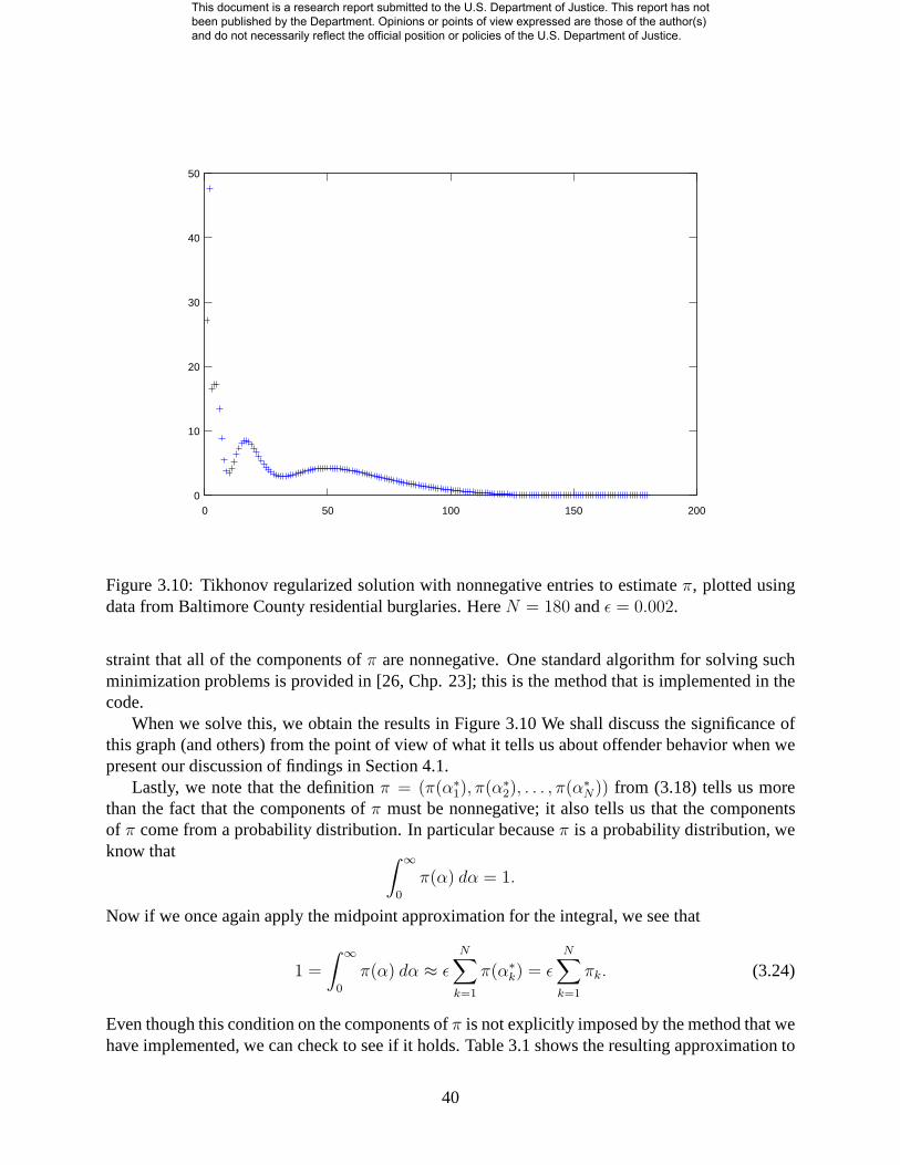
100 150 2000

10

20

0 50

30

40

50

Figure 3.10: Tikhonov regularized solution with nonnegative entries to estimateπ, plotted usingdata from Baltimore County residential burglaries. HereN = 180 andε = 0.002.

straint that all of the components ofπ are nonnegative. One standard algorithm for solving suchminimization problems is provided in [26, Chp. 23]; this is the method that is implemented in thecode.

When we solve this, we obtain the results in Figure 3.10 We shall discuss the significance ofthis graph (and others) from the point of view of what it tells us about offender behavior when wepresent our discussion of findings in Section 4.1.

Lastly, we note that the definitionπ = (π(α∗1), π(α∗

2), . . . , π(α∗N)) from (3.18) tells us more

than the fact that the components ofπ must be nonnegative; it also tells us that the componentsof π come from a probability distribution. In particular becauseπ is a probability distribution, weknow that

∫ ∞

0

π(α) dα = 1.

Now if we once again apply the midpoint approximation for the integral, we see that

1 =

∫ ∞

0

π(α) dα ≈ ε

N∑

k=1

π(α∗k) = ε

N∑

k=1

πk. (3.24)

Even though this condition on the components ofπ is not explicitly imposed by the method that wehave implemented, we can check to see if it holds. Table 3.1 shows the resulting approximation to

40


Solution method Estimate of∫∞0

π(α) dα

Pseudoinverse -5896180Tikhonov regularization 0.970644Nonnegative least squares without regularization 1.074468Nonnegative least squares with Tikhonov regularization 0.973170

Table 3.1: Estimates of∫∞0

π(α) dα for various solution methods, calculated from BaltimoreCounty residential burglary data withN = 180 andε = 0.002

∫∞0

π(α)dα generated by (3.24) for various solution methods. We see that in each case we do havethe appropriate rough approximation, save for the solution generated directly by the pseudoinverse,which we have already seen to be wildly inaccurate (Figure 3.5). However, no error analysis hasyet been performed on these values. It is an interesting open question to see what better methodsmight be to perform the estimate of the functionπ(α).

3.2.4 The geographic triangulation

We now turn to the problem of representing the local geometry and geography. To do so, we startby realizing that there are three geographic regions that interest us

1. The crime region. We assume all of the known crimes are contained in a single geographicregion, which we call the crime region. In particular, we assume that we have no informationabout whether or not the offender has committed additional series crimes outside the crimeregion. If an agency is investigating a crime series, and has no information about the seriesfrom other jurisdictions, then the crime region is just the jurisdiction of the investigatingagency. If more than one agency is cooperating and sharing data, then the crime region willbe the region formed by all of the jurisdictions sharing data.

2. The home base region. The home base region needs to be chosen sufficiently large tocontain the anchor point of the offender; it must also contain the entire crime region. In ourprogram, the home base region will be one or more county sized regions as selected by theprogram user.

3. The search box. This is the smallest rectangle that contains the crime region and the homebase region.

The coarse mesh

As our first step in the geographic analysis, we will cover the search box with a coarse triangularmesh. Let the circumradius of the triangles in the coarse mesh beRcoarse= R. We assume that thegrid contains:

• m rows of triangles, withm odd, and

• n columns of triangles, withn even.

41


Figure 3.11: Relationships between crime region, home base region, and the search box

n (even)

m(o

dd

)

WidthWSearch Box

HeightH

Figure 3.12: Coarse triangular mesh and the search box

42


R√

3

3R

2

R

R/2

R√

3/2

R

Figure 3.13: Dimensions of a typical triangle

To ensure that the coarse grid covers the search box, we place the top left corner of the searchbox at the centroid of the triangle in the first row and first column, as seen in Figure 3.12. Then,examining the size of each individual triangle, we see that to ensure that the search box remainsentirely within the triangulated mesh, we need

(n2− 1)R

√3 ≥ W

(m − 1)(3R/2) ≥ H

As a consequence, we choose

m odd,m > 1 +2H

3R= 2 +

2H3Rcoarse

,

n even,n > 2 +2W

R√

3= 4 +

2WRcoarse

√3.

Area of a coarse mesh triangle In addition to the geometric dimensions of the coarse trian-gle shown in Figure 3.13, we will also need the areaA of these triangles; for reference we simplynote that

A =1

2

3R

2R√

3 =3√

3

4R2.

Finding the orientation of the coarse mesh’s triangles Label each triangle in the mesh by apair of nonnegative integers(i, j), where this refers to the triangle in theith column and thej th row;for consistency with our C++ code, we start these indices with zero, soi ∈ {0, 1, 2, . . . , n−1} andj ∈ {0, 1, . . . , m − 1}. We count the columns starting from the left edge working right, and wecount the rows starting from the top and working downward.

Each triangle in the mesh has a side that is parallel to thex-axis. We say that the triangle pointsdownward if they-coordinate of the centroid is smaller that they-coordinate of the side that is

43


parallel to thex-axis; otherwise we say that the triangle points upward. We call this the orientationof the triangle.

Examining Figure 3.12, we see that

• i + j = even if and only if the triangle points downward;

• i + j = odd if and only if the triangle points upward.

Finding the centroids of the coarse mesh’s triangles Suppose that the coordinates(x0, y0) ofthe top left corner of our search box are known. How can we find the coordinates of the centroidsof all of the triangles in the coarse mesh?

Consider a triangle in the mesh at position(a, b) with center(x, y). Then choose(α, β), and askwhat are the coordinates of the center of the triangle whose position in the mesh is(a+α, b+β) =(i, j). If α + β is even, then both the triangle(a, b) and the triangle(a + α, b + β) both have thesame orientation, and so

coordinates of(a + α, b + β) are(x, y) + R(

α√

32

, β(−3

2

)

)

,

because each triangle has widthR√

3/2 and height3R/2 (see Figure 3.13) and because we countrows going downward.

On the other hand, ifα + β is odd, thenα + β − 1 is even, and so

coordinates of(a + α, b + β − 1) are(x, y) + R(

α√

32

, (β − 1)(−3

2

)

)

.

Then, ifa+b is even, the original triangle pointed downward and so our new triangle points upwardand hence


α√

32

, (β − 1)(−3

2

)

)

+ (0,−2R).

On the other hand, ifa + b is odd, then the original triangle pointed upward and our new trianglepoints downward; then


α√

32

, (β − 1)(−3

2

)

)

+ (0,−R).

With these calculations in hand, we can use the fact that the top left corner of the mesh(x0, y0)is the centroid of the triangle in position(0, 0); thus the triangle is position(i, j) has centroid

• (x0, y0) + R(

i√

32

, j(−3

2

)

)

if i + j is odd, and

• (x0, y0) + R(

i√

32

, (j − 1)(−3

2

)

− 1)

if i + j is even.

These are the calculations that are used in our code, specifically in the constructorCTriangulatedGeography::CTriangulatedGeography .

44


(x0, y0) (x0, y0) + R(√

3, 0)(x0, y0) + R(√

32

, 0)

(x0, y0) + R(√

32

,−32)

(x0, y0) + R(3√

34

,−34)(x0, y0) + R(

√3

4,−3

4)

u=

R(0,−

32 )

v =R( 3 √

34 ,− 3

4 )

w=

R(3√ 3

4,34)

Figure 3.14: Vectorsu, v, andw for a typical triangle in the coarse mesh

45


(0, 0) (2, 0) (4, 0) (6, 0)

(1, 0) (3, 0) (5, 0) (7, 0)

(0, 1) (2, 1) (4, 1) (6, 1)

(1, 1) (3, 1) (5, 1) (7, 1)

(0, 2) (2, 2) (4, 2) (6, 2)

(1, 2) (3, 2) (5, 2) (7, 2)

(0, 3) (2, 3) (4, 3) (6, 3)

(1, 3) (3, 3) (5, 3) (7, 3)

α = 0

α = 1

α = 2

α = 3

β=

0β

=1

β=

2β

=3

γ=−

1

γ=

0

γ=

1

γ=

2

Figure 3.15: Coordinates in the coarse mesh

Determining the coarse mesh triangle containing a point Given a point with known coordi-nates(x, y), we would like to be able to determine the coordinates(i, j) of the coarse mesh trianglethat contains that point. To do so, define the vectorr = (x − x0, y − y0) and consider the vectors

u = R(0,−32) v = R(3

√3

4,−3

4) w = R(3

√3

4, 3

4)

which are shown in Figure 3.14. Note that|u|2 = |v|2 = |w|2 = 9R2/4.Calculate the projection ofr in the directions ofu, v, andw, so that

α =

⌊

r · u|u|2

⌋

, β =

⌊

r · v|v|2

⌋

, γ =

⌊

r · w|w|2

⌋

where we have rounded each fraction to the largest integer lower than the given fraction. Thenexamining Figure 3.15, we see that the triplet(α, β, γ) then gives us our location within the mesh,and the coordinates(i, j) of the triangle are then found by simply calculating

i = β + γ j = α.

Determining the coarse mesh triangle near a point Suppose that a point(x0, y0) is known, andwe want to find all of the coarse mesh triangles within a distanceρ from (x0, y0). How we proceeddepends on the relationship betweenρ andR.

46


Figure 3.16: Determining the coarse mesh triangles near a point; ρ < R.

Small distances In the case whereρ < R, we begin by drawing circles of radiusR centeredat the three vertices of the triangle. Because every point in the triangle is a convex combination ofthe three vertices, it suffices to then take the convex hull of the resulting three circles; this is donein figure 3.16.

Suppose that(x0, y0) is in the coarse mesh triangle with coordinates(i0, j0). If this triangleis oriented upwards, then examining the figure, we see that all points within a distanceρ < R of(x0, y0) lie in the triangles with coordinates:

• (i0 − 2, j0), (i0 − 2, j0 + 1)

• (i0 − 1, j0 − 1), (i0 − 1, j0), (i0 − 1, j0 + 1)

• (i0, j0 − 1), (i0, j0), (i0, j0 + 1)

• (i0 + 1, j0 − 1), (i0 + 1, j0), (i0 + 1, j0 + 1)

• (i0 + 2, j0), (i0 + 2, j0 + 1)

while if the triangle containing(x0, y0) is oriented downwards, then all points within a distanceρ < R of (x0, y0) lie in the triangles with coordinates:

• (i0 − 2, j0 − 1), (i0 − 2, j0)

• (i0 − 1, j0 − 1), (i0 − 1, j0), (i0 − 1, j0 + 1)

• (i0, j0 − 1), (i0, j0), (i0, j0 + 1)

• (i0 + 1, j0 − 1), (i0 + 1, j0), (i0 + 1, j0 + 1)

• (i0 + 2, j0 − 1), (i0 + 2, j0)

47


(x0, y0)

(x, y)

0 R√

32

2R√

32

3R√

32

4R√

32

5R√

32

6R√

32

7R√

32

0

3R2

23R2

33R2

43R2

b

b

Figure 3.17: Distances in the coarse mesh

Large Distances To handle the situation whereρ ≥ R, let us consider the situation where

• (x0, y0) is in the triangle(i0, j0),

• (x, y) is in the triangle(i, j), and

• dist((x0, y0), (x, y)) ≤ ρ.

Define the numbers∆i = |i − i0|, ∆j = |j − j0|. Examining Figure 3.17, we can see that

(∆i − 2)R√

3

2≤ |x − x0| ≤ (∆i + 2)

R√

3

2,

(∆j − 1)3R

2≤ |y − y0| ≤ (∆j + 1)

3R

2.

Thus

(∆i − 2)R√

3

2≤ |x − x0| ≤ dist((x0, y0), (x, y)) ≤ ρ

(∆j − 1)3R

2≤ |y − y0| ≤ dist((x0, y0), (x, y)) ≤ ρ

so that

∆i ≤ 2 +2ρ√3R

∆j ≤ 1 +2ρ

3R.

Thus, we set

∆i = 2 +

⌈

2ρ√3R

⌉

∆j = 1 +

⌈

2ρ

3R

⌉

48


Then, given the triangle(i0, j0), all of the triangles(i, j) that contain a point of distance no morethanρ from triangle(i0, j0) satisfy

|i − i0| ≤ ∆i |j − j0| ≤ ∆j

Though fast to implement, this method is not sharp. For example, ifρ < R, then this methodreturns all triangles with|i − i0| ≤ 3 and|j − j0| ≤ 2, which is a larger set than what we returnedabove.

The fine mesh

Differing quantities of interest vary on very different distance scales. For example, the targetattractivenessG(x) from (3.10) may vary dramatically from one block to another. Other functions,like the normalization functionN(x) from (3.9) vary much more slowly. If we were to try touse a single mesh for all of our calculations, we would either lose accuracy because the mesh istoo coarse for the rapidly varying functions, or we would lose performance because we would becalculating essentially the same slowly varying variables over and over.

Our solution is to use two different meshes, the coarse grid which we have already described,and another finer mesh, which we will obtain by subdividing the coarse mesh triangles.

Triangular coordinates To construct our fine mesh, we subdivide each triangle from the coarsemesh intoN2 subtriangles. We then need to determine the characteristics of each of these subtri-angles from our knowledge of the characteristics of the original, coarse mesh triangle. To do so,we start by introducing the usual set of triangular coordinates. To do so, label the vertices asv1,v2, v3. Then a pointx in the triangle has triangular coordinates(α, β, γ) if and only if

x = αv1 + βv2 + γv3

whereα + β + γ = 1.We then split the collection of subtriangles into those with the same orientation as the parent

triangle and those with the opposite orientation as the parent triangle. See Figures 3.18 and 3.20;note that the orientation of the parent triangle is irrelevant though the parent triangle in these figuresis shown with an upward orientation for definiteness in the figure and the following discussion.

Subtriangles with the same orientation as the parent We begin by considering the subcollec-tion of subtriangles with the same orientation as the parent. Examining Figure 3.18, we see thatthere are

∑Ni=1 i = 1

2N(N + 1) such subtriangles. We index each subtriangle by the triangular co-

ordinates of the bottom left corner of the subtriangle. For anyi, j, k satisfyingi+j+k = N , j ≥ 1andi, k ≥ 0, the point(i/N, j/N, k/N) is the bottom left corner of a triangle in our subcollection.This condition oni, j, k is equivalent to the requirements

• 0 ≤ i ≤ N − 1,

• 1 ≤ j ≤ N − i, and

• k = N − i − j

49


(0, 1, 0)

(1, 0, 0)

(0, 0, 1)

Figure 3.18: Subdivided coarse triangle- subtriangles with the same orientation

( iN

, jN

, kN

)

( iN

, jN

, kN

) + ( 1N

, −1N

, 0)

( iN

, jN

, kN

) + (0, −1N

, 1N

)

( iN

, jN

, kN

) + ( 13N

, −23N

, 13N

)

Figure 3.19: Calculating the centroid of a subtriangle

50


(0, 1, 0)

(1, 0, 0)

(0, 0, 1)

Figure 3.20: Subdivided coarse triangle- subtriangles with the opposite orientation

We also notice that the vector from the bottom left corner to the centroid of the subtriangle is, intriangular coordinates, the vector( 1

3N, −2

3N, 1

3N); this follows immediately from Figure 3.19. Thus,

the centroid of the triangle with bottom left corner(i/N, j/N, k/N) is ( iN

, jN

, kN

) + ( 13N

, −23N

, 13N

).

Subtriangles with the opposite orientation as the parent Examining figure 3.20, we see thatthere are

∑N−1i=1 i = 1

2(N − 1)N subtriangles whose orientation is opposite to that of the parent.

We index these subtriangles by the triangular coordinates of their bottom vertex. Then, for anyi, j, k satisfyingi + j + k = N , j, k ≥ 1, i ≥ 0, the point(i/N, j/N, k/N) is the bottom vertex ofa triangle in our subcollection. This condition oni, j, k is equivalent to the requirements

• 0 ≤ i ≤ N − 2,

• 1 ≤ j ≤ N − i − 1, and

• k = N − i − j.

We also notice that the vector from the bottom vertex to the centroid of the subtriangle is, intriangular coordinates, the vector(−2

3N, 1

3N, 1

3N); this follows immediately from Figure 3.21. Thus,

the centroid of the triangle with bottom vertex(i/N, j/N, k/N) is ( iN

, jN

, kN

) + (−23N

, 13N

, 13N

).

Cartesian Coordinates Now that we have determined the triangular coordinates for the cen-troids of all of the subtriangles, we need to determine their corresponding Cartesian coordinates. Todo so, we begin by finding Cartesian coordinates of the point with triangular coordinates(α, β, γ)with α + β + γ = 1 for a parent triangle with centroid(x0, y0) and circumradiusR.

Examining Figure 3.22, we see clearly that the result will depend on the orientation of theparent triangle. In the case where the parent triangle has an upward orientation (as was the de-fault shown in Figures 3.18 and 3.20) we see that we have the following relationship between theCartesian and triangular coordinates of the vertices of the parent triangle

51


( iN

, jN

, kN

) + ( 1N

, 0, −1N

)

( iN

, jN

, kN

)

( iN

, jN

, kN

) + ( 1N

, −1N

, 0)

( iN

, jN

, kN

) + ( 23N

, −13N

, −13N

)

Figure 3.21: Calculating the centroid of a subtriangle

(1, 0, 0) = (x0, y0) + R(0,−1)

(0, 1, 0) = (x0, y0) + R(−√

32

,−12) (0, 0, 1) = (x0, y0) + R(

√3

2,−1

2)

(0, 1, 0) = (x0, y0) + R(−√

32

, 12) (0, 0, 1) = (x0, y0) + R(

√3

2, 1

2)

(1, 0, 0) = (x0, y0) + R(0, 1)

(13, 1

3, 1

3) = (x0, y0)

(13, 1

3, 1

3) = (x0, y0)

Figure 3.22: Converting from triangular coordinates to Cartesian coordinates. Left: Parents with adownward orientation. Right: Parents with an upward orientation

52


Parent oriented upwardsCartesian Coordinate Triangular Coordinate

(1, 0, 0) (x0, y0) + R(0, 1)

(0, 1, 0) (x0, y0) + R(−√

32

,−12)

(0, 0, 1) (x0, y0) + R(√

32

,−12)

As a consequence, the Cartesian coordinates for the point with triangular coordinates(α, β, γ) ina parent triangle with upward orientation are

(α, β, γ) 7→ (x0, y0) + R(−√

32

β +√

32

γ, α − 12β − 1

2γ).

On the other hand, if the parent triangle has a downward orientation, then we have the following

Parent oriented downwardsCartesian CoordinateTriangular Coordinate

(1, 0, 0) (x0, y0) + R(0,−1)

(0, 1, 0) (x0, y0) + R(−√

32

, 12)

(0, 0, 1) (x0, y0) + R(√

32

, 12)

As a consequence, the Cartesian coordinates for the point with triangular coordinates(α, β, γ) ina parent triangle with downward orientation are

(α, β, γ) 7→ (x0, y0) + R(−√

32

β +√

32

γ,−α + 12β + 1

2γ).

3.2.5 Evaluating the probability densityP (z)

Our goal is to determine the probability densityP (z) that the offender’s anchor point is located atthe pointz. Of course, this function is defined for every value ofz. Rather than calculate this forevery value ofz however, we will only calculate it for the pointsz that are the centroid of a trianglein our fine mesh.

3.2.6 The Normalization Function

The normalization functionN(z, α) defined by (3.9)

N(z, α) =

[∫∫

R2

D(x | z, α)G(x) dx(1)dx(2)

]−1

. (3.25)

is effectively impossible to evaluate analytically, and very difficult to do so numerically. However,it does possess some properties that will enable us to evaluate it more efficiently. As we will befocusing in the integral rather than on its inverseN , we adopt the notation

I(z, α) =

∫∫

R2

D(x | z, α)G(x) dx(1)dx(2)

in what follows.

53


The Tail

First, we notice thanks to the definition ofG(x) in (3.10), there is an absolute constantΓ so that

0 ≤ G(x) ≤ Γ

for all x ∈ R2. We also note that the graph off(r |α) has a single positive maximum after whichit decays rapidly; see Figure 3.2. In particular, we note that

max f(r |α) =1

α

√

π

2e≈ 0.760173

α,

arg max f(r |α) = α

√

2

π≈ 0.797885α.

To actually evaluateI(z, α), we begin by replacing the region of integration by the region[|x − z| < R] for someR. The resulting error is

∣

∣

∣

∣

∫∫

R2

D(x | z, α)G(x)dx−∫∫

[|x−z|<R]

D(x | z, α)G(x)dx

∣

∣

∣

∣

=

∫∫

[|x−z|≥R]

D(x | z, α)G(x)dx

≤ 2πΓ

∫ ∞

R

r

4α2exp

(

−πr2

4α2

)

dr

≤ Γ exp

(

−πR2

4α2

)

The exact value ofI(z, α) is unknown, so we are unable to estimate the relative error; however if

G(x) ≈ λΓ for all x, then the integral is approximatelyλΓ; thus we use the factorexp(

−πR2

4α2

)

as

a proxy for the relative error.In particular, if we want out estimate for the relative error caused by neglecting the tail to satisfy

exp

(

−πR2

4α2

)

≤ 10−k

thenπR2

4α2≥ k ln 10

so we choose

R ≥ 2

√

ln 10

π

√kα ≈ 1.71223

√kα.

Reasonable values are

54


b

(0, R)

(−R√

32

,−R2) (R

√3

2,−R

2)

(0, 0)

Figure 3.23: Discretization of an integral

10−k Rcrit

10−1 1.71223α10−2 2.42146α10−3 2.96567α10−4 3.42447α10−5 3.82687α10−6 4.19410α10−7 4.53014α10−8 4.84293α

The discretization

To evaluate the portion of the integral excluding the tail,i.e. the portion of the integral for which|x − z| < R, we use the two-dimensional midpoint rule.

The two-dimensional midpoint rule For simplicity, we start by describing how to evaluate theintegral of an arbitrary functionf(x, y) over an equilateral triangle with centroid at the origin andcircumradiusR, as seen in figure 3.23

Let T be our equilateral triangle; then for any(x, y) ∈ T , there is a point(x0, y0) ∈ T so thatTaylor’s Theorem will let us write

f(x, y) = f(0, 0) +∂f

∂x(0, 0)x +

∂f

∂y(0, 0)y

+1

2

(

∂2f

∂x2(x0, y0)x

2 + 2∂2f

∂x∂y(x0, y0)xy +

∂2f

∂y2(x0, y0)y

2

)

55


We now integrate both sides in(x, y) overT .A simple symmetry argument shows that

∫∫

T

∂f

∂x(0, 0)x dx dy = 0

On the other hand

∫∫

T

∂f

∂y(0, 0)y dx dy = 2fy(0, 0)

∫ R

−R/2

∫ −√

3

3(y−R)

0

y dx dy

= 2fy(0, 0)

∫ R

−R/2

−√

3

3y(y − R) dy

= −2√

3

3fy(0, 0)

[

1

3y3 − 1

2Ry2

]R

−R/2

= −2√

3

3fy(0, 0)

[

1

3R3 +

1

3

(

R

2

)3

− 1

2RR2 +

1

2R

(

R

2

)2]R

−R/2

= −2√

3

3fy(0, 0)

[

1

3+

1

24− 1

2+

1

8

]

R3 = 0.

Thus,∫∫

T

f(x, y) dx dy = A(T )f(0, 0) + E

whereA(T ) is the area of triangleT , and the errorE satisfies

E =1

2

∫∫

T

(

∂2f

∂x2(x0, y0)x

2 + 2∂2f

∂x∂y(x0, y0)xy +

∂2f

∂y2(x0, y0)y

2

)

so that

|E| ≤ 1

2‖fxx‖∞

∫∫

T

x2 dx dy + ‖fxy‖∞∫∫

T

|xy| dx dy +1

2‖fyy‖∞

∫∫

T

y2 dx dy

Now direct evaluation shows us that∫∫

T

x2 dx dy =3√

3

8R4

∫∫

T

y2 dx dy =3√

3

8R4

∫∫

T

|xy| dx dy =15

32R4

and consequently

|E| ≤(

15

16+

3√

3

4

)

∥

∥D2f∥

∥

∞ R4

56


We will then use the midpoint approximation

∫∫

T

f(x, y) dx dy =

(

3√

3

4R2

)

f(0, 0) + O(R4)

to evaluate our integral.

Application to the normalization function Now

I(z, α) =

∫∫

R2

D(x | z|, α)G(x) dx(1) dx(2) =

∫∫

R2

1

4α2exp

(

− π

4α2|x − z|2

)

G(x) dx(1) dx(2)

Let ∆ be a collection of equilateral triangles whose closures cover the plane and whose interiorsare disjoint. Then, we can rewrite the integral above as∫∫

R2

D(x | z|, α)G(x) dx(1) dx(2) =∑

T∈∆

∫∫

T

1

4α2exp

(

− π

4α2|x − z|2

)

G(x) dx(1) dx(2).

Using the midpoint method, we then obtain the approximation

∫∫

R2

D(x | z|, α)G(x) dx(1) dx(2) ≈ 3√

3

16

1

α2

∑

T∈∆

R2T exp

(

− π

4α2|xT − z|2

)

G(xT )

whereRT is the circumradius andxT is the centroid of the triangleT .

Selecting the mesh

We begin by selecting a circumradius of the coarse mesh triangles,Rcoarse. Based on our analysisof the tail, we see that relative error in replacing the integral overR2 with the integral over thesmaller region[|x − z| < 3α] is roughlye−9π/4 ≈ 0.000851. Thus, we shall drop from the mesh∆ any triangleT for which |xT − z| > 3α

We also see that the relative error in replacing the integral overR2 with the integral over theeven smaller region[|x − z| < 2α] is roughlye−π ≈ 0.0432. Because this is not insignificant, wewill retain all of the triangles for which2α < |xT − z| ≤ 3α.

Finally, our analysis of the tail tells us that the vast majority of the contributions to our integralcome from the region|xT − z| ≤ 2α. For this reason, we subdivide all of the coarse triangles inthis region into their corresponding fine subtriangles before evaluating the integral.

This is the process that is used in the code to evaluateI(z, α).

Evaluating I(z, α) asz varies

Although we have outlined how we are able to evaluate the integralI(z, α), we do not want to doso for every potential value ofz. As described in Section 3.2.5, we only need to evaluateP (z)and henceI(z) for pointsz that are the centroids of triangles in the fine mesh. However, this turnsout to be impractical, as the computation time to evaluateI(z) even once is significant. Testinghas shown that this process, simplified as it was in the previous discussion, is still by far the mostcomputationally expensive portion of the algorithm.

57


Rather than use this algorithm at the centroid of every fine triangle, we instead use this methodonly to calculate the values ofI(z) on the vertices of the coarse triangles and interpolate into thefine triangles within.

Suppose we are given a coarse triangleT and the values ofI at the vertices ofT ; and want touse interpolation to approximate the values ofI in the interior ofT . Let c be the center andR thecircumradius of the coarse triangleT ; then the vectors fromc to the vertices ofT are

v1 = ±R 〈0, 1〉

v2 = ±R

⟨√3

2,−1

2

⟩

v3 = ±R

⟨

−√

3

2,−1

2

⟩

where the+ sign is chosen when the triangle is oriented upwards and the− sign when the triangleis oriented downwards. The vertices ofT are then{c + vi}3

i=1.We then examine the known values ofI on the vertices ofT , naming them

I1 = I1(α) = I(c + v1, α),

I2 = I2(α) = I(c + v2, α),

I3 = I3(α) = I(c + v3, α).

Now select a pointz ∈ T , and letx = z− c; then

x = t1v1 + t2v2 + t3v3

z = c + t1v1 + t2v2 + t3v3

where

ti =1

3+

2

3

x · vi

R2.

Indeed

z = c + t1v1 + t2v2 + t3v3

= c + 13(v1 + v2 + v3) + 2

31

R2 {(x · v1)v1 + (x · v2)v2 + (x · v3)v3}= c + 2

31

R2 {(x · v1)v1 + (x · v2)v2 + (x · v3)v3}= c + 2

3

{

〈0, x2〉 +(√

32

x1 − 12x2

)⟨√3

2,−1

2

⟩

+(

−√

32

x1 − 12x2

)⟨

−√

32

,−12

⟩}

= c + 23

{

〈0, x2〉 +⟨

32x1,

12x2

⟩}

= c + x = z.

as required.Thus, for any pointz ∈ T , we calculate the numbersti and use the linear approximation

I(z, α) ≈ t1I1 + t2I2 + t3I3.

58


Evaluating I(z, α) asα varies

The approximation ofI(z, α) by linear interpolation within a coarse triangle does not always pro-duce reasonable results; in fact the accuracy of the approximation deteriorates asα ↓ 0.

Recall thatα is the average distance the offender is willing to travel and that the dependenceonz of the integrand is through (3.11),

D(x | z, α) =1

4α2exp

(

−π

4

[ |x − z|α

]2)

.

Examining this, we see that ifz1 andz2 are far apart relative toα, then|x− z1|/α and|x− z2|/αare very different, and soI(z1, α) andI(z2, α) are likely different.

Since the coarse triangles have circumradiusR = Rcoarse, if R � α, then the variation in theintegrand overT is small, and the interpolation should provide reasonable approximations; on theother hand ifR � α, then the variation of the integrand overT is large, and we expect poorapproximations. This has been observed in numerical results.

To proceed, we write the integral as

I(z, α) =

∫∫

R2

D(x | z, α)G(x)dx(1)dx(2)

=1

4α2

∫∫

R2

exp

(

−π

4

|x − z|2α2

)

G(x)dx(1)dx(2)

Setξ = 12α

(x − z), thendξ = 14α2 dx so

I(z, α) =

∫∫

R2

exp(−π|ξ|2)G(z + 2αξ) dξ.

From this we can clearly see thatI(α) → G(z) asα ↓ 0.Continuing our analysis, we can replaceG by its Taylor series; then

I(z, α) =

∫∫

R2

exp(−π|ξ|2){

G(z) + 2α DG(z) · ξ + 4α2ξ>D2G(z)ξ + O(α3)}

dξ.

Note that the second term vanishes; indeed∫∫

R2

exp(−π|ξ|2)DG(z) · ξ dξ =

∫ 2π

0

∫ ∞

0

e−πr2|DG(z)|r cos θ · r dr dθ = 0

whereθ is the angle measured from the directionDG(z)/|DG(z)|. Thus, we can write

I(z, α) ≈ G(z) + c2(z)α2 + O(α3)

for smallα.With this in mind, we wish to approximateI(z, α) for α near 0 by interpolation. We suppose

that we already have approximations forI(z, α) for α = α1 < α2 < · · · < αN , but that theaccuracy of the approximations diminishes asα ↓ 0.

59


We begin by choosingK so large that our approximations are reasonable atαk for k ≥ K. Inparticular, we chooseK so large thatα∗

K ≥ 2R, that is

α∗K = (K − 1

2)ε ≥ 2R

so we wantK ≥ 1

2+ 2(R/ε)

To proceed, we use the Hermite approximation

A(α) = ω0 + ω1(α − αK) + ω2(α − αK)2 + ω3α(α − αK)2

so thatA′(α) = ω1 + 2ω2(α − αK) + ω3(α − αK)2 + 2ω3α(α − αK).

The coefficientsω0, ω1, ω2 andω3 are chosen so that

A(0) = I(z, 0) A(αK) = I(z, αK)

A′(0) =∂I

∂α(z, 0) A′(αK) =

∂I

∂α(z, αK)

From our Taylor series approximations nearα = 0, we concluded

I(z, 0) = G(z)∂I

∂α(z, 0) = 0.

The value ofI(z, αK) we have from our approximations, while we use

∂I

∂α(z, αK) ≈ I(z, αK+1) − I(z, αK)

ε.

Now

A(0) = ω0 − αKω1 + α2Kω2 A(αK) = ω0

A′(0) = ω1 − 2αKω2 + α2Kω3 A′(αK) = ω1

so we set

ω0 = I(z, αK)

ω1 = 1ε[I(z, αK+1) − I(z, αK)]

ω2 = 1α2

K

[G(z) − ω0 + αKω1]

ω3 = 1α2

K

[2αKω2 − ω1]

This is the method that is used in the code to evaluate the integralsI(z, α).

60


3.3 Reprise of mathematical assumptions and computationaltechniques

Assumption Comments Location

The offender chooses offense locationsaccording to a probability distributionP (x | z, α) that depends only on the of-fender’s anchor pointz and the average dis-tanceα the offender is willing to travel tooffend.

This is fundamental to our approach, thoughthe mathematical framework allows for thepossibility that P depends on other vari-ables.

page 17

The offender’s choices of crime sites aremathematically independent of one another

This is a required mathematical simplifi-cation for (3.4); without it one must alsomodel the nature and form of the effect ofthe choice of one crime site has on the of-fender’s selection of subsequent crime sites.

page 19

The offender’s distance decay function is in-dependent of the offender’s anchor point

This is a required mathematical simplifica-tion for (3.2); without it one must also modelthe nature and form of the dependence of theaverage offense distance on the location ofthe offender’s anchor point.

page 19

The probability densityP has the formP (x | z, α) = D(d(x, z), α)G(x)N(z, α)

Other reasonable forms for this probabilitydensity exist and can be treated via thesemathematical techniques; this is the selec-tion that was implemented in the softwareprototype.

page 20

The offender’s two-dimensional distancedecay function is a normal distributionD(x | z, α) = 1

4α2 exp(

− π4α2 |x − z|2

)

This is the choice made in the software pro-totype. Other reasonable choices exist, likethe negative exponential.

pages 21,26

The likelihood that a particular location willbe the location of a future offense can beestimated from the locations of historicalcrimes of the same type as the offense.

In the prototype software, the analyst needsto select the historically similar crimes.

page 22

The distribution of anchor points follows lo-cal population density for people with thesame age / sex / race or ethnic group of theoffender

The prototype software uses U.S. Censusdata to perform the calculations.

page 23

The prior distribution of average offense dis-tancesπ(α) can be calculated by using his-torical data and solving (3.15)

This is difficult to solve in practice; see com-putational techniques.

page 28

Table 3.2: Summary of mathematical assumptions in the model

61


Technique LocationEquation (3.15) which is used to determine the estimate for the distribution ofaverage offense distances across offenders is solved by using collocation to convertit to a linear system, which is then solved via Tikhnonv regularization.

Subsection3.2.3

The continuous functions in the model are estimated by calculating their values ona triangular grid that overlays the geographic region under consideration. The gridis kept at two levels of detail, a coarse grid and a fine sub-grid.

Subsections3.2.4 and 3.2.5

The integral defining the normalization functionN(z, α) is evaluated at each pointin the coarse grid using the midpoint method, where the precise mesh used is anadaptive combination of elements from the coarse mesh and the fine mesh depend-ing on the value ofα. These values are interpolated into the fine mesh via geometricinterpolation and Hermite approximation inα.

Subsection3.2.6

Table 3.3: Summary of computational techniques in the software

3.4 The software

3.4.1 Overview

We have developed software that implements these mathematical algorithms. The software wasbuilt in two parts:

• A program called Profiler that performs all of the mathematical analysis, and

• A program called ProfilerGUI with which the user interacts.

The software was developed in this fashion for a number of reasons. First and foremost, thisapproach allows this scientific work to be kept separate from user interface issues. In particular,because the scientific analysis is performed in a separate, stand-alone program, it is possible forthis tool to be incorporated into other software suites that have compatible open source licenses.In addition, this approach lets us work separately on the user interface and the scientific analysistools.

To use the software, the user starts ProfilerGUI; a screen shot is contained in Figure 3.24.The user interface then prompts the user to enter the required data for the program. When this iscomplete, ProfilerGUI writes a plain text parameter file that contains all of the user’s selections.ProfilerGUI then calls the program Profiler, and passes it the name of the parameter file it justwrote. Profiler performs its analysis; as it returns information this is noted by ProfilerGUI andreported to the user. It total, the program provides

• A map of the proposed search area, in .kml format,

• A map of the target attractiveness functionG(x), in .kml format, and

• A map of the population density of the search area that matches the provided demographicinformation, again in .kml format.

62


Figure 3.24: Screenshot of the Program

63


Because the analysis process can take some time- a few hours istypical, the program also providesthe analyst with its partial results as the analysis continues.

The output maps are provided in .kml format; this is an open standard. Files in this format canbe rendered by a number of free programs, including

• Google Earth,

• ESRI’s ArcGIS Explorer, and

• NASA’s World Wind.

All of the maps in this report are screen shots taken from Google Earth.In this section, we will describe first how the program is installed, including how to obtain all

of the required files. We will then provide step-by-step instructions on how the program is meantto be used. Finally, we will take a brief look at the source code for the two software tools, andexplain how they have been designed and built.

3.4.2 Installing the software

The software tool comes packaged as a compressed .zip archive. Once downloaded, the user simplyneeds to uncompress the archive to create a folder called Profiler; see Figure 3.25 as an example.

At this point, the tool is ready to run; just use the ProfilerGUI program provided in the rootdirectory. No other installation tasks need to be performed.

3.4.3 Using the software

Detailed instructions on the use of the program have been provided with the software in the formof a .pdf sideshow that illustrates the use of the program on a series of convenience store robberiesin Baltimore County. In this report, we shall briefly summarize the process.

Selecting the crime series

The first step is to select the crime series under analysis. The program requires a plain text filethat contains the locations of the crime series. Each line of this file contains the longitude andlatitude of one element of the crime series, separated by one or more spaces. Both longitude andlatitude are specified in decimal degrees, and need to be separated by one or more spaces. The filename can be entered either by directly typing its name into the Crime Series box or by pressing thecorresponding Select File button to obtain a dialog box that allows the user to simply click on thedesired file.

Selecting the historical crime locations

Next, the analyst needs to provide a plain text file that contains the locations of a representative setof crimes of the same type as the series under consideration. This file has the same structure as thecrime series file, save that each line now contains the longitude and latitude of a single historicalcrime.

64


Figure 3.25: Unpacking the software archive

65


This is the information that the algorithm uses to generate its estimate forG(x). The crimesused in the historical crime locations may be solved or unsolved, and need not be from seriescrimes. Not every crime of the same type needs to be included, just enough to generate a repre-sentative sample. As part of the analysis, the program will generate a map of the resulting targetattractivenessG(x); it is important that this map be checked for reasonableness.

In particular, the bandwidth used to generate the map of historical crimes is twice the meannearest neighbor distance between offenses. Thus, if too few historical crime sites are included,then the mean nearest neighbor distance will be large, and so the graph will be very broad andsmooth- perhaps broader and smoother than the analyst feels is appropriate. As a consequence,when deciding what historical crimes to use, the analyst needs to balance how well the historicalcrimes match the series versus the need to have a representative sample that generates a reasonablemap of historical crimes.

It is also important to note that regions where the historical crime locations map is zero areconsidered to be regions where there can be no known crimes in the series known to the analyst. Aconsequence of this is that if an analyst is investigating a series that crosses multiple jurisdictions,then the analyst needs to have the corresponding historical information for all of these jurisdictions.

Selecting the historical distances

To create the estimate of the prior distribution of offender average offense distances, the programrequires a plain text file that contains the locations of a representative set of solved crimes togetherwith the location of the offender’s home base. This file has the same structure as the crime seriesfile, save that each line now contains the longitude and latitude of a crime site together with thelongitude and latitude of the offender’s home base.

The solved crimes used to generate the historical distances do not need to be of exactly the sametype as the series under consideration. They only need to provide a reasonable basis to estimatethe distance decay function for offenders in the jurisdiction.

Selecting the search region

The search region is composed of one or more county-sized regions. The list of available county-sized regions is taken from the U.S. Census. The analyst simply needs to select the state andcorresponding county sized region(s) from the available drop boxes. Up to four different regionscan be selected.

When selecting the search region, it is important to note that the algorithm will assume that theoffender is not located outside of the search region. In particular, the search area chosen at thisstage must be sufficiently large to encompass the anchor point of any potential offender. Failure todo so will result in search areas that are strongly biased.

To perform its analysis, the program needs to possess the necessary U.S. Census data for theselected regions. When a region is selected, the program will check to see if it has the necessarydata files. If it does not, then a message will be displayed, explaining the issue. The box tells theuser the name of the files that are needed, provides a link to the Census web site from which thefiles can be downloaded, and indicates the locations where the downloaded data files need to bestored. It is impractical to distribute all of the required data files directly with the program due

66


to their large size. Indeed, if we were to include the necessary census data for all fifty states, theresult would be many hundreds of times the size of the program.

Selecting the offender information

If the age, sex, or race / ethnic group of the offender is known to the analyst, this informationcan be included. When the program develops its prior estimate for the distribution of potentialoffender anchor pointsH(z) before the information from the crime series is taken into account, ituses population density data from the U.S. Census for this purpose. Because the Census providesblock level data subdivided by age, sex, and race /ethnic group, we can use that information whendeveloping this prior estimate. Entering the available data is done by simply choosing from theappropriate drop boxes; the default assumption is that no demographic information is availableabout the offender.

Program results

As we have already noted, the program produces a number of maps as its output, including a mapof the search area, a map of the target attractiveness function, a map of the population density,and interim maps of the search area as the analysis proceeds. All of these results are stored in thedirectory that the user specifies here, either by directly entering the name of the directory, or byusing the dialog box obtained by pressing the Select Directory button.

The analysis

Once all of the necessary data has been entered, the Start Analysis button will be enabled; oncepressed the program will begin its work. First the program will read the necessary data files andinitialize internal data structures; as this process occurs, the status bar will keep the user informed.When the initialization is complete, the program will begin by working one subregion at a time andcalculating the probability that the offender’s anchor point lies in that subregion. The total numberof subregions searched is recorded as a fraction of the total number of subregions in the searcharea, as well as the relative likelihood of the last searched subregion as a fraction of the maximumlikelihood so far encountered.

Now an exhaustive search of every possible subregion would significantly increase computationtime to no real benefit- given that the search area is the size of one or more counties, most of thesubregions are unlikely to contain the offender’s anchor point. Instead, the search proceeds byspiraling out from the crime series, and continuing until it can make a complete circuit where thethe likelihood that any of the subregions in the circuit contains the offender’s anchor point is lessthan 0.5% of the most likely subregion. The Estimated Progress bar tracks how close the programhas come to making a complete circuit where all of the subregion likelihoods have remained belowthis threshold. If during this process the program encounters a subregion where the likelihoodis larger than this threshold, then it must begin a new circuit at this point and so the EstimatedProgress bar will drop back to 0%.

67


Running time

The software prototype is computationally intensive, and the process can take quite some timeto complete. In Chapter 4, we apply the software prototype to a series of 6 convenience storerobberies in Baltimore County. When the prototype is run on a new Windows Vista system (Core2 Duo T6400, 4 GB memory) for this series, the program needs roughly an hour and a half tocomplete. The same series when analyzed on an older Windows XP system (Pentium D 805, 2GBmemory) has a run time of roughly two hours; older systems have even longer run times.

Despite the long run times for the software prototype, it is designed to be run while other ap-plications also run on the system without using all of the computer’s resources. Thus, the machineshould not “freeze” or become unresponsive while the prototype is running, and other applicationscan be used concurrently with the prototype.

3.4.4 Internal structure of the software

Profiler

Profiler is a program written entirely in C++ to implement our mathematical algorithms. It is a con-sole based program that is usually run in concert with ProfilerGUI, but can also be run separatelyas a stand-along program.

Using Profiler as a stand-alone program To run Profiler as a stand-alone program, it needsto be run from the command line with the name of a plain text file that contains the parametersnecessary for the analysis; if no parameter is passed the program looks for the parameter file withname./Parameters/Parameters.txt .

A typical parameter file looks like the following

Triangle Circumradius = 0.01Crime Series Data File Name = ./Parameters/series.txtHistorical Data File Name = ./Parameters/history.txtHistorical Distances File Name = ./Parameters/historical_distances.txtNumber of regions = 2State = MDCounty Code = 005State = MDCounty Code = 510Race / Ethnic group = Asian aloneSex = FemaleMinimum Age = 0Maximum Age = MaximumResults Directory = ./Results

An explanation of the individual parameters follows

• Triangle Circumradius : The geographic region under study is subdivided into a mesh ofequilateral triangles (the coarse mesh), and each of these triangles is then subdivided into anumber of subtriangles, resulting in the fine mesh. The size of the triangles in the coarsemesh is the input variable Triangle Circumradius.

68


Figure 3.26: Screenshot of Profiler running as a stand-alone program

69


• Crime Series Data File Name: This is the name of a plain text file that contains the longi-tude and latitude of each element of the crime series.

1. Each line of the file should contain the latitude and longitude of a single crime location.

2. The latitude and longitude should be separated by one or more blank spaces, withlongitude first, and latitude last.

3. The latitude and longitude should be specified in decimal degrees.

4. The file should contain no other data; in particular it should not end with a blank line.

• Historical Data File Name: This is the name of a plain text file that contains the longitudeand latitude of historical crimes of the same type as the series under study.

1. The historical data is used to generate a map of the relative likelihood that a particularlocation is the site of a crime of the same type as the that series under study. The dataset should be sufficiently large for this purpose.

2. The historical data does not need to consist of solved crimes, nor does the historicaldata need to consist of series crimes.

3. Each line of the file should contain the latitude and longitude of a single crime location.

4. The latitude and longitude should be separated by one or more blank spaces, withlongitude first, and latitude last.

5. The latitude and longitude should be specified in decimal degrees.


• Historical Distances File Name: This is the name of a plain text file that contains thelongitude and latitude of both the locations of a crime and the home base of the offender.

1. The historical data is used to generate a graph of crime frequency versus distance.

2. The historical data should be from crimes similar to the series under consideration.

3. Each line should contain the data from a single historical crime, and should contain inorder the longitude and latitude of the crime site, then the longitude and latitude of thehome base of the offender.

4. The latitudes and longitudes should be separated from each other by one or more blankspaces.

5. The latitudes and longitudes should be specified in decimal degrees.


• Number of regions: This is the number of county-equivalent regions that are necessary tocontain both the all of the elements of the crime series as well as the largest possible searcharea

• State: Two letter abbreviation for a state containing a county-sized region to be searched.

70


• County Code: This is the corresponding three digit U.S. Census Bureau County Code1; thisdoes not include the associated two digit state code.

• Race / Ethnic group: This is the Race or Ethnic group of the offender; the classificationscheme is the same as that which is used by the U.S. Census Bureau in Summary File 12.

• SexThis is the sex of the offender.

• Minimum Age This is a lower estimate for the possible age of the offender. Not every choiceof age is valid; the value needs to be the lower bound for an age range for which the U.S.Census records block level population data; see Summary File 1.

• Maximum Age This is a upper estimate for the possible age of the offender. Not everychoice of age is valid; the value needs to be the upper bound for an age range for which theU.S. Census records block level population data.

• Results Directory: This is the name of the directory that the program will use to store itsresults.

Compiling Profiler This program was compiled with gcc(3.4.5)/MinGW; it also requires theLapack++ libraries (2.5.1). It is important to use the a recent version of Lapack++. There is amuch older version (1.1a) of Lapack++ available at the NIST web site; it is not suitable.

Brief overview of the Profiler source code Profiler was developed using a strict object-orientedapproach; its functions were split into twelve distinct classes:

• Input and output classes

– CInput is used to handle all of the input to the program; it reads the parameter file, aswell as any auxiliary data files and performs all validation.

– COutput is used to generate all of the maps developed by the code in.kml format.

– CCensus is used to read data from U.S. Census data files.

• Auxiliary classes for data

– CBlock is an auxiliary class that encapsulates a U.S. census block.

– CPt is an auxiliary class that encapsulates a geographic point.

– CTriangle is an auxiliary class that represents a triangular geographic region.

• Classes for geography

– CTriangulatedGeography is the main class that handles the geography. Thegeographic region under study is covered by two triangular meshes, a coarse mesh thatis used for functions that vary slowly and are difficult to compute- likeN(z, α), anda much finer mesh for functions that vary much more rapidly- likeG(x) andH(z),which can change dramatically from block to block.

1http://www.census.gov/datamap/fipslist/AllSt.txt2http://www.census.gov/Press-Release/www/2001/sumfile1.html

71


http://www.census.gov/datamap/fipslist/AllSt.txt

http://www.census.gov/Press-Release/www/2001/sumfile1.html

• Functions in the mathematical model

– CDistanceDecay is the class that contains the data for the distance decay functionD; it also contains the results for the prior distribution of offender average offensedistanceπ(α).

– CNormalizationFunction is the class that calculates the values of the normal-ization functionN(z, α).

– CTargetDensity is the class that contains the values for the target density functionG(x).

– CPopulation is the class that contains the data forH(z).

– CTikhonov is the class that is used to perform the regularization process, it is anauxiliary class forCDistanceDecay , and reports its results back to that class forstorage.

Now we briefly describe each class used by Profiler.

CBlock This class is a data structure to hold the elements of a U.S. Census Bureau blockthat are relevant for the code. This data is all available in Summary File 1. In particular, the classrecords

• The U.S. Census Bureau logical record number of the block,

• The land area of the block, in square meters,

• The latitude and longitude of the block (in degrees), and the

• Population of the block.

The population recorded inCBlock is not necessarily the total population of the block, but ratherthe population for the combination of age, sex, and race / ethnic group under consideration.

CCensus This class that contains all of the census data for the county or counties that containthe potential search area.

The Census Bureau Summary file 1 has block level population data for each county in thecountry, sorted by age, sex, and race / ethnic group. For each state, we require three files:

• STgeo.uf1

• ST00005.uf1

• ST00006.uf1

where ST is replaced by the corresponding two letter state abbreviation. These files must be in-cluded in the same directory as the program executable; they can be directly downloaded from theU.S. Census site.

The demographic information- age, sex, and race/ethnic group follow the Census Bureau stan-dard definitions and groupings.

72


Internally, the class stores an array of blocks (typeCBlock ) which contain the location, landarea, and population (in the specified demographic) of each block.

This data is be used byCPopulation to construct the prior distribution for anchor pointsH(z).

CDistanceDecay This class handles both the explicit form of the distance decay function aswell as the creation of the prior estimate for the distance decay function.

All distances are measured in decimal degrees. The motivation for this choice is the fact thatsince the input latitude and longitude will be in degrees, it makes more sense to keep the sameunits throughout.

The implementation of the distance between two points is actually handled by theCPt::S2DistanceTo function, and work on the assumption that the Earth’s surface is spherical. Inparticular, no correction factors for the ellipsoidal nature of Earth have (yet) been incorporated.

The primary mathematical quantities that this class needs to store are the arrays

• αk, the values ofα at which the priorπ is recorded,

• πk ≈ π(αk), the values of the prior estimate for the distance decay function, and

• ∆αk ≡ αk+1 − αk, the increments inα

To evaluate the later integrals, only the nonzero values ofπk are needed; hence the class stores thevalues of the triples(αk, πk, ∆αk) for only the non-zero values ofπk.

This data structure also allows for the possibility of adaptive integration inα by adjusting thestep sizes∆αk, but right now all of these values are constant.

CInput This is the class used to set up and handle all of the input and output files for theprogram. The constructor is passed the program’s arguments; it uses these to determine the locationof the parameter file, which it then opens. The constructor then reads the parameter file, and storesall of the necessary results in class variables.

The class provides a family of functions that provide to access the parameters, which are storedin class variables.

CNormalizationFunction This class handles all of the calculations necessary to evaluateN(z, α).

It has one public member function, which is used to actually calculate the integral. It startswith a valuez and an array{α1, α2, . . . , αK}, then returns the array of values

{N−1(z, α1), N−1(z, α2), . . . , N

−1(z, αK)},

whereN−1(z, α) is defined by

N−1(z, α) =

∫∫

R2

D(d(x, z))G(x) dx(1) dx(2)

This is done by adaptive integration and uses the private functionCNormalizationFunction::GetOneMeshValue The private function chooses a triangulation of the region of inte-gration that depends on the values ofαi and then performs the integration.

73


COutput This class is used to generate and write all of the output maps produced by theanalysis engine. To create an instance, you must specify the output type and the file name ofthe output. Right now, only .kml output formats are supported. The constructor creates the filewith the provided name in the directory recorded in theCOutput::resultsDirectory . Theconstructor also writes the required elements of the .kml header.

Function calls can then be made toCOutput::DrawPoint andCOutput::DrawGraphso that data can be added to the output. Multiple maps can be overlaid in the same output file;the altitude of each map is stored in the class variableCOutput::altitude , and this value isincreased by 50 each timeCOutput::DrawGraph is called.

The destructor∼COutput writes the KML footer and closes the file.

CPopulation This class stores the population data for the search region. This is used as aproxy for an estimate of the prior distribution of offender anchor points.

Right now, this is calculated only from US Census data; in the future we would like to use otherdata sets (e.g. distributions of other offenders) to generate this distribution. This can be done mostsimply by overloading the constructor.

CPt This class forms a data structure for a two-dimensional point. Implemented operationsinclude the standard vector operations (addition, scalar multiplication), the (Euclidean) dot productand Spherical distance (CPt::S2DistanceTo ).

CTargetDensity This class is used as a data structure to hold the target density functionG(x). In particular, this class calculates and stores the value ofG(x) at the centers of the finetriangles in the mesh; these values can be retrieved viaCTargetDensity::getFineValue .

The class also calculates and stores the value ofG(x) for each coarse triangle. Rather thansimply calculate the value ofG(x) at the center point of the coarse triangle, it instead uses theaverages of the values ofG at all of the fine triangle contained within the coarse triangle. Thereason for this behavior is that the underlying functionG varies on a very fine scale. It makessense that to calculate the value ofG on the fine mesh, because that is the finest mesh in theproblem. When looking for the value ofG at for a coarse triangle, if we simply calculated thevalue ofG at the center of the triangle, then we run the risk that a small change in the locationof the center of the coarse triangle can result in a large change in the value returned. Instead, wereturn the average value to try to smooth our the results.

The values ofG(x) are calculated using a kernel density estimation process. In particular,suppose that the historical crimes have been committed at the locationsc1, c2, . . . , cN . Considerthe truncated quartic kernel functionK(x|λ) with bandwidthλ

K(x|λ) =

3

πλ6(|x|2 − λ2)2 if |x| ≤ λ

0 if |x| ≥ λ

The bandwidthλ is chosen to be twice the mean nearest neighbor distance between historicalcrimes, and

G(x) ∝N∑

i=1

K(x − ci|λ).

74


CTikhonov This class is used solely to compartmentalize the process of calculating the non-negative Tikhonov regularized solution to a linear equation. It uses the mathematical algorithmsdescribed in Section 3.2.3.

CTriangle This is a data structure for a triangle with sides parallel to thex-axis. It retainsthe center of the triangle, its circumradius, and its orientation, where the orientation determines ifthe centroid is above or below the side parallel to thex-axis.

CTriangulatedGeography This is a data structure that contains all of the underlying ge-ographic structure of the program. The class contains two primary data structures- a mesh ofcoarse triangles and a mesh of fine triangles. Each of the triangles in the coarse mesh are of typeCTriangle , meaning that they are equilateral and have one side parallel to thex-axis. Thiscoarse grid covers the entire geographic region under consideration, including the crimes, the his-torical crimes, and the region to be searched.

Each coarse triangle is subdivided into subtriangles, also of classCTriangle .The coarse grid and the fine grid are entirely created by the constructor; the primary public

methods return various grids, sub-grids, and individual triangles.

ProfilerGUI

ProfilerGUI is a program written in C++ to provide a simple interface to allow an analyst to in-teract with the Profiler program. ProfilerGUI requires the presence of the program Profiler in asubdirectory of the same name. When ProfilerGUI runs, it takes the data provided by the user,writes a parameter file, calls Profiler, and then interprets the results returned by Profiler.

Compiling ProfilerGUI This program was developed with the GPL version of Qt Creator 1.1.1,based on Qt 4.5.1. It requires no additional libraries beyond those included in Qt Creator.

Brief overview of the ProfilerGUI source code This program is designed to take full advantageof the signals and slots mechanisms provided by Qt. In particular, this allows us to create an event-driven program where actions taken in the user interface (e.g. pressing a button or editing a box)cause code to be executed.

The program contains only two classes-MainDlg andCStatus , and nearly all of the workoccurs inMainDlg . This is the class that handles the program’s primary dialog. It is responsiblefor

• Displaying the dialog (and all sub-dialogs, including file/directory selection and help di-alogs)

• Recording all of the entered data

• Starting the profiler (analysis) program

• Reading the data returned by the profiler program, and updating the user on the status of theanalysis.

75


The classCStatus is simply a data structure containing five boolean variables where eachvariable represents the status of one of the required data elements-

• The crime series,

• The history file,

• The historical distances file,

• The search region, and

• The results directory.

When true they indicate that the GUI program has the necessary data for that data element.The public functionCStatus::Prepared returns true if all of the status variables are true;

otherwise it returns false. It is used to determine if the program is ready to allows the analysiscomponent to run.

Integrating Profiler and ProfilerGUI When complete, the software package contains

• ProfilerGUI.exe

• The file counties.txt, which is a modified version of a list of county codes provided by theU.S. Census.

• Two .dll files from the Qt library:

– QtCore4.dll

– QtGui4.dll

• The analysis program (Profiler.exe) and its associated files in the Profiler subdirectory. Inparticular, the subdirectory needs to contain

– Profiler.exe

– Three lapack++ library files:

∗ libblas32.dll

∗ liblapack32.dll

∗ liblapackpp-15.dll

76


Chapter 4

Results

4.1 Discussion of findings

The purpose of our project was to develop a new mathematical approach for the geographic profil-ing problem and to implement that new algorithm in software, and we have done so. To illustratehow our model and tools work in practice, let us consider a series of convenience store robberiesthat occurred in Baltimore County in May 2008.

Basic information about the crime series is provided in Table 4.1, and the crime locations aremapped in Figure 4.1. Note that crimes 1, 4 and 6 all occurred at the same location marked asCrime Site # 6 on the map. To give this information to our program, we simply provide it with aplain text file containing the latitude and longitude of each crime site.

As we begin our analysis, we start with the elementary observation that not every location canbe the site of a convenience store robbery- after all not every location is the site of a conveniencestore. Instead, experience tells us that convenience stores tend to be concentrated at or near majorintersections. Moreover, some convenience stores are more likely to be the site of a robbery thanothers. To account for these geographic facts, our algorithm requires the locations of a representa-tive sample of the locations of convenience store robberies throughout the jurisdiction. A simplegraph of the locations of convenience store robberies in Baltimore County is provided in Figure4.2. Even though this figure does not include the locations of the major roadways, the target patternclearly shows where many of them lie.

Date TimeLocation

TargetLatitude Longitude

March 8 12:30 pm -76.71350 39.29850 Speedy MartMarch 19 4:30 pm -76.74986 39.31342 ExxonMarch 21 4:00 pm -76.76204 39.34100 ExxonMarch 27 2:30 pm -76.71350 39.29850 Speedy MartApril 15 4:00 pm -76.73719 39.31742 CitgoApril 28 5:00 pm -76.71350 39.29850 Speedy Mart

Table 4.1: A series of convenience store robberies in Baltimore County

77


Figure 4.1: Convenience store robbery series in Baltimore County

78


Figure 4.2: Convenience store robberies in Baltimore County

79


Figure 4.3: Target attractiveness for convenience store robberies in Baltimore County

Another important geographic factor in the analysis of this series is the presence of the jurisdic-tional boundary. Baltimore County and Baltimore City are separate jurisdictions, and the elementsof the crime series under consideration lie very close to this boundary. This particular series wasidentified by Baltimore County, and though there are no known elements of the series in the city,this cannot be ruled out.

Thus, we provide the program with another plain text file, this one containing the locationsof 449 convenience store robberies within the county. The program then calculates the resultingtarget attractiveness functionG(x), and returns it to the analyst; this map is shown in Figure 4.3

Our goal is to obtain an estimate of the location of the offender’s anchor point; if we assume thatthe anchor point is a residence, then we immediately know that there are locations where the anchorpoint cannot be located. For example, looking at the crime series map (Figure 4.1), we see that eastof the crime series locations is a large park, near the crime sites is a large interstate overpass and acommercial area including offices and a number of malls, and to the west is a wooded area. Sincenone of these areas contain residences, none of these areas are likely to contains the offender’s

80


Figure 4.4: Population density and proposed anchor point density near the crime series

residence. To handle this geographic information, our method uses local population density fromU.S. Census data as a proxy for anchor point density. In particular, our existing software is able toread the raw data from the census and use a modified kernel density parameter estimation techniqueto generate a map of potential anchor points; it is shown in Figure 4.4.

One advantage of using census data is that population data is available at the block level sortedby age, sex, and race or ethnic group. Thus, if demographic information about the offender isavailable, then it too can be incorporated into our analysis. For example, notice the differences inthe population density maps for different racial / ethnic groups shown in Figure 4.5.

Another fundamental factor of interest is the distance decay function of an offender. Our mathe-matical method does not make ana priori choice of the offender’s distance decay function. Instead,our method assumes that different offenders have different average offense distances. We providethe program with the locations of both the offense site and the home of 751 solved robberies. Theprogram then performs the analysis described in Section 3.2.3, and generates the distribution ofaverage offense distances across offenders that is shown in Figure 3.10.

81


(a) Asian (b) Black

(c) Hispanic (d) White

Figure 4.5: Population density for different race / ethnic groups

82


Figure 4.6: Proposed search area

When our software prototype is run on this series, we obtain the search area in Figure 4.6Notice that the calculated search area avoids parks and commercial areas, while at the same timefollowing the local road network. Note also that the regions considered most likely to contain theoffender’s residence do not lie in the region bounded by the crime sites, but rather lie towards thecenter of the city; compare this with the comments about the convex hull effect made by Levine[28].

The algorithm that generates the search area uses the local population density, so it knowsthat there are more potential offenders nearer to the city center than farther away. In addition,the algorithm is also aware of the jurisdictional boundaries; in particular it takes into account thepossibility that elements of the series may have been committed in the city but that these elementsare unknown to the analyst. Together, these facts suggest that the offender is more likely to livecloser to the city, and the calculated search area agrees.

The potential impact of demographic information about the offender is clearly illustrated in

83


Figure 4.7 which show what the search area would be if we had information about the race orethnic group of the offender. It is clear to see that the search areas have significant differences.

4.2 Implications for policy and practice

Our primary motivation for this project is to improve the operational efficiency of law enforcementagencies as they search for serial offenders by providing them with better and more sophisticatedtools. This we have done; the software we have developed in now freely available on our websiteat http://pages.towson.edu/moleary/Profiler.html .

We presented our first functional prototype software package at the NIJ Conference in June2009. The program is now being used by both the Los Angeles Police Department and the Balti-more County Police Department, both of whom are examining the effectiveness and usefulness ofthe tool.

It should be noted however, that we have not yet made a study of the effectiveness of the toolor of the mathematical algorithms that it contains.

On the other hand, by making our mathematics, algorithms and code widely and publicly avail-able, we also hope that we can provide valuable insights to other researchers. We also have writtena manuscript that describes the mathematical techniques that we have used; this is currently underreview at the Journal of Investigative Psychology and Offender Profiling.

4.3 Implications for further research

There are a number of important areas in which research in this area should be continued. First, theeffectiveness of the our tool needs to be measured. The first prototype version was just released inJune; it will take some time to collect the necessary data to see if this will result in any significantimprovement over the current generation of techniques for geographic profiling.

Second, we need to remove some of the limitations that currently exist in the software proto-type. For example, Phil Canter of the Baltimore County Police Department has indicated that thesoftware prototype would be much more useful if the range of output file formats was increased.In particular, he has asked us to develop the capability to return results in either a plain text format,or even better in a Shapefile format so that the results can be better integrated into their existingGIS infrastructure. Sean Malinowski, of the Los Angeles Police Department asked if it wouldbe possible to use geographical information that describes the distribution of known offenders inplace of Census data to generate the estimate of the prior distribution of offenders. We hope tobegin work on both of these suggestions soon so that we can get an improved tool into the handsof these agencies.

The mathematical framework we have developed for the geographic profiling problem is quitebroad, and there are a number of reasonable forms for many of the distributions that are used in themodel. To name just one example, our software tool posits that the distance decay componentDfollows a bivariate normal distribution, but clearly this is not the only reasonable alternative. Weneed to go back and start examining and evaluating different options for all of these distributions,and comparing them and their effectiveness. The tools of model selection and multimodel inferencehave yet to be applied to this problem, and may be able to generate some new insights.

84


http://pages.towson.edu/moleary/Profiler.html

(a) Asian (b) Black

(c) Hispanic (d) White

Figure 4.7: Proposed search area for offender of different race / ethnic groups

85


Finally, the mathematical model of offender behavior described inP (x | z, α) remains quitesimple. A new preprint by Mohler and Short [36] shows how they have developed an approach togeographic profiling where the simple probabilistic models for the distance decay component ofoffender behavior are replaced by the results of random walks. This is an innovative new idea thatdeserves significant additional study.

86


Bibliography

[1] Martin Baxter and Andrew Rennie,Financial calculus, Cambridge University Press, 1996.

[2] Mokhtar S. Bazaraa, Hanif D. Sherali, and C.M. Shetty,Nonlinear programming, John Wileyand Sons, 2006.

[3] Edward J. Beltrami,Mathematical models in the social and biological sciences, Jones andBartlett Publishers, 1993.

[4] Craig Bennell, Brent Snook, and Paul Taylor,Geographic profiling- The debate continues,Blue Line Magazine (2005), 34–36.

[5] Craig Bennell, Brent Snook, Paul Taylor, Shevaun Corey, and Julia Keyton,It’s no riddle,choose the middle, Criminal Justice and Behavior34 (2007), no. 1, 119–132.

[6] Wim Bernasco and Paul Nieuwbeerta,How do residential burglars select target areas? Anew approach to the analysis of criminal location choice, British Journal of Criminology45(2005), no. 3, 296–315.

[7] Patricia L. Brantingham and Paul J. Brantingham,Residential burglary and urban form, Ur-ban Studies12 (1975), no. 3, 273–284.

[8] , Nodes, paths and edges: considerations on the complexity of crime and the physicalenvironment, Journal of Environmental Psychology13 (1993), 3–28.

[9] Marilyn A. Brown, Modelling the spatial distribution of suburban crime, Economic Geogra-phy (1982), 247–261.

[10] Thiess Buettner and Hannes Spengler,Local determinants of crime: Distinguishing be-tween resident and non-resident offenders, Darmstadt Discussion Papers in Economics 120,Institut fr Volkswirtschaftslehre (Department of Economics), Technische Universitt Darm-stadt (Darmstadt University of Technology), February 2003, Online athttp://ideas.repec.org/p/tud/ddpiec/120.html .

[11] David Canter, Toby Coffey, Malcolm Huntley, and Christopher Missen,Predicting serialkillers’ home base using a decision support system., Journal of Quantitative Criminology16(2000), no. 4, 457–478.

[12] David Canter and P. Larkin,The environmental range of serial rapists, Journal of Environ-mental Psychology13 (1993), 63–69.

87


http://ideas.repec.org/p/tud/ddpiec/120.html

http://ideas.repec.org/p/tud/ddpiec/120.html

[13] Bradley P. Carlin and Thomas A. Louis,Bayes and empirical Bayes methods for data analy-sis, 2nd ed., Chapman & Hall / CRC, 2000.

[14] George Casella and Roger L. Berger,Statistical inference, 2nd ed., Duxbury, 2002.

[15] Spencer Chainey,Methods and techniques for understanding crime hot spots, MappingCrime: Understanding Hot Spots, The National Institute of Justice, Washington DC, August2005, pp. 15–34.

[16] Warren John Ewens,Mathematical population genetics, Springer Verlag, 2004.

[17] Katarina Fritzon,An examination of the relationship between distance travelled and moti-vational aspects of firesetting behaviour, Journal of Environmental Psychology21 (2001),no. 1, 45–60.

[18] Elizabeth Groff and Nancy G. La Vigne,Mapping an opportunity surface of residential bur-glary, Journal of Research in Crime and Delinquency38 (2001), no. 3, 257–278.

[19] Per Christian Hansen,Rank-deficient and discrete ill-posed problems, SIAM, 1998.

[20] David Kincaid and Ward Cheney,Numerical analysis, second ed., Brooks Cole, 1996.

[21] Richard N. Kocsis, Ray W. Cooksey, Harvey J. Irwin, and Greg Allen,A further assessmentof circle theory for geographic psychological profiling, The Australian and New ZealandJournal of Criminology35 (2002), no. 1, 43–62.

[22] Richard N. Kocsis and Harvey J. Irwin,An analysis of spatial patterns in serial rape, ar-son, and burglary: The utility of the circle theory of environmental range for psychologicalprofiling, Psychiatry, Psychology and Law4 (1997), 195.

[23] Peter J. Van Koppen and Jan W. de Keijser,Desisting distance decay: On the aggregation ofindividual crime trips, Criminology35 (1997), 505.

[24] Peter J. Van Koppen and Robert W. J. Jansen,The road to robbery. Travel patterns in com-mercial robberies, British Journal of Criminology38 (1998), no. 2, 230–246.

[25] Manne Laukkanen and Pekka Santtila,Predicting the residential location of a serial com-mercial robber, Forensic Science International157(2006), no. 1, 71–82.

[26] Charles L. Lawson and Richard J. Hanson,Solving least squares problems, SIAM, 1995.

[27] James L. LeBeau,The methods and measures of centrography and the spatial dynamics ofrape, Journal of Quantitative Criminology3 (1987), no. 2, 125–141.

[28] Ned Levine, The evaluation of geographic profiling software: Response to KimRossmo’s critique of the NIJ methodology, Online at http://www.nedlevine.com/ResponsetoKimRossmoCritiqueoftheGPEvaluationMethodology.May82005.doc , (Accessed July 2009), 2005.

88


http://www.nedlevine.com/Response to Kim Rossmo Critique of the GP Evaluation Methodology.May 8 2005.doc



[29] , CrimeStat: A spatial statistics program for the analysis of crime incident loca-tions (v. 3.2), Online at http://www.icpsr.umich.edu/crimestat , (AccessedJuly 2009), 2009.

[30] , Update notes to version 3.2. CrimeStat: A spatial statistics program for the analysisof crime incident locations, Online athttp://www.icpsr.umich.edu/crimestat ,(Accessed July 2009), 2009.

[31] Ned Levine and Richard Block,Bayesian journey to crime estimation: An improvement ingeographic profiling methodology, Professional Geographer, to appear.

[32] Manuel J.J. Lopez,The spatial behavior of residential burglars, Proceedings of the 5th SpaceSyntax Symposium (A. van Nes, ed.), Techne Press, 2005, pp. 423–435.

[33] Yongmei Lu,Getting away with the stolen vehicle: an investigation of journey-after-crime,The Professional Geographer55 (2003), no. 4, 422–433.

[34] Jacek Malczewski, Anneliese Poetz, and Luigi Iannuzzi,Spatial analysis of residential bur-glaries in London, Ontario, The Great Lakes Geographer11 (2004), no. 1, 15–27.

[35] Rebecca Meaney,Commuters and marauders: An examination of the spatial behavior ofserial criminals, Journal of Investigative Psychology and Offender Profiling (2004), 121–137.

[36] George O. Mohler and Martin B. Short,Geographic profiling from kinetic models of crimi-nal behavior, Online athttp://www.math.ucla.edu/ ˜ gmohler/geopro2.pdf ,(Accessed July 2009).

[37] Denise R. Osborn and Andromachi Tseloni,The distribution of household property crimes,Journal of Quantitative Criminology14 (1998), no. 3, 307–330.

[38] Jerry H. Ratcliffe,A temporal constraint theory to explain opportunity-based spatial offend-ing patterns, Journal of Research in Crime and Delinquency43 (2006), no. 3, 261–291.

[39] George F. Rengert, Alex R. Piquero, and Peter R. Jones,Distance decay reexamined, Crimi-nology37 (1999), 427–445.

[40] Tom Rich and Michael Shively,A methodology for evaluating geographic profiling software,Tech. report, Abt Associates, Cambridge, MA, 2004.

[41] Kim Rossmo,Geographic profiling, CRC Press, 2000.

[42] , An evaluation of NIJ’s evaluation methodology for geographic pro-filing software, Online at http://www.txstate.edu/gii/documents/ResponsetoNIJGPEvaluationMethodology.doc , (Accessed July 2009), 2005.

[43] , Geographic heuristics or shortcuts to failure?: Response to Snook et. al., AppliedCognitive Psychology19 (2005), 651–654.

[44] Kim Rossmo and Scot Filer,Analysis versus guesswork, Blue Line Magazine (2005), 24,26.

89


http://www.icpsr.umich.edu/crimestat

http://www.icpsr.umich.edu/crimestat

http://www.math.ucla.edu/~gmohler/geopro2.pdf

http://www.txstate.edu/gii/documents/Response to NIJ GP Evaluation Methodology.doc

http://www.txstate.edu/gii/documents/Response to NIJ GP Evaluation Methodology.doc

[45] Kim Rossmo, Scot Filer, and Carl Sesley,Geographic profiling debate- round four. The bigproblem with Bennell, Snook and Taylor’s research, Blue Line Magazine (2005), 28–29.

[46] Bernard Silverman,Density estimation for statistics and data analysis, CRC Press, 1986.

[47] Brent Snook,Individual differences in distance travelled by serial burglars, Journal of Inves-tigative Psychology and Offender Profiling1 (2004), no. 1, 53–66.

[48] Brent Snook, David Canter, and Craig Bennell,Predicting the home location of serial offend-ers: A preliminary comparison of the accuracy of human judges with a geographic profilingsystem, Behavioral Sciences & the Law20 (2002), 109–118.

[49] Brent Snook, Paul Taylor, and Craig Bennell,Geographic profiling: The fast, frugal, andaccurate way, Applied Cognitive Psychology18 (2004), no. 1, 105–121.

[50] , Man versus machine. The case of geographic profiling, Blue Line Magazine (2005),56.

[51] , Shortcuts to geographic profiling success: A reply to Rossmo, Applied CognitivePsychology19 (2005), 655–661.

[52] Brent Snook, Michele Zito, Craig Bennell, and Paul J. Taylor,On the complexity and accu-racy of geographic profiling strategies, Journal of Quantitative Criminology21 (2005), no. 1,1–26.

[53] Andromachi Tseloni, Karin Wittebrood, Graham Farrel, and Ken Pease,Burglary victim-ization in England and Wales, the United States, and the Netherlands, British Journal ofCriminology44 (2004), no. 1, 66–91.

[54] Curtis R. Vogel,Computational methods for inverse problems, SIAM, 2002.

[55] Fahui Wang and W. William Minor,Where the jobs are: Employment access and crimepatterns in Cleveland, Annals of the Association of American Geographers92 (2002), no. 3,435–450.

[56] Janet Warren, Roland Reboussin, Robert R. Hazelwood, Andrea Cummings, Natalie Gibbs,and Susan Trumbetta,Crime scene and distance correlates of serial rape, Journal of Quanti-tative Criminology14 (1998), no. 1, 35–59.

[57] R. Clyde White,The relation of felonies to environmental factors in Indianapolis, SocialForces10 (1931), 498–509.

[58] Paul Wiles and Andrew Costello,The road to nowhere: the evidence for travelling crim-inals, Tech. report, Home Office Research Study 207, 2000, Online athttp://www.homeoffice.gov.uk/rds/pdfs/hors207.pdf , accessed July 2009.

[59] Paul Wilmott,Derivatives, John Wiley and Sons, 1998.

[60] Paul Wilmott, Sam Howison, and Jeff Dewynne,The mathematics of financial derivatives,Cambridge University Press, 1995.

90


http://www.homeoffice.gov.uk/rds/pdfs/hors207.pdf

http://www.homeoffice.gov.uk/rds/pdfs/hors207.pdf

[61] B. J. Worton,Kernel methods for estimating the utilization distribution in home-range studies,Ecology70 (1989), no. 1, 164–168.

91


Dissemination of Research Findings

Articles

• Mike O’Leary. The Mathematics of Geographic Profiling, under review at the Journal ofInvestigative Psychology and Offender Profiling

Presentations

• A new software tool for geographic profiling, The NIJ Conference, Arlington, VA, June 2009

• Mathematical models for the geographic profiling problem, Center for Evidence Based CrimePolicy, George Mason University, March 2009

• Mathematical models for the geographic profiling problem, Georgetown University Mathe-matics Department Colloquium, March 2009

• Determining the Optimal Search Area for a Serial Criminal, Joint Mathematics Meetings,Washington DC, January 2009.

• Advances in Geographic Profiling, 31st Applied Geography Conference, Wilmington DE,October 2008.

• Determining the Optimal Search Area for a Serial Criminal, INFORMS National Meeting,Washington DC, October 2008.

• The Mathematics of Geographic Profiling, The NIJ Conference, Arlington VA, July 2008

• The Mathematics of Geographic Profiling, Spring Meeting, Geospatial Technology WorkingGroup, New Orleans LA, April 2008.

• The Mathematics of Geographic Profiling, Center for Army Analysis, Fort Belvoir, April2008

92


List of Supplemental Material

• The software tool, as a .zip archive

• Instructions for the use of the software tool, as a .pdf slide show

• The source code for the Profiler program

• Browseable documentation for the source code of the Profiler program in web / html format

• Printable documentation for the source code of the Profiler program in .pdf format

• The source code for the ProfilerGUI program.

• Browseable documentation for the source code of the ProfilerGUI program in web / htmlformat

• Printable documentation for the source code of the ProfilerGUI program in .pdf format

93


a new mathematical approach to geographic profiling new mathematical approach to geographic...

Documents