a new implementation to the vehicle type scheduling ... · vehicle-type scheduling problem (vtsp)....

XLVSBPOSetembro de 2013

Natal/RN

16 a 19Simpósio Brasileiro de Pesquisa OperacionalA Pesquisa Operacional na busca de eficiência nosserviços públicos e/ou privados

A NEW IMPLEMENTATION TO THE VEHICLE TYPE SCHEDULING PROBLEM

WITH TIME WINDOWS FOR SCHEDULED TRIPS

Monize Sâmara Visentini

Universidade Federal do Rio Grande do Sul (UFRGS)

Rua Washinton Luiz, 855. Porto Alegre, R.S.

[email protected]

Denis Borenstein



[email protected]

Olinto César Bassi de Araújo

Universidade Federal de Santa Maria (UFSM)

Avenida Roraima, 1000. Santa Maria, R.S.

[email protected]

Pablo C. Guedes



[email protected]

ABSTRACT

Kliewer et al. (2006b, 2011) proposed a time window implementation to the multi-depot

vehicle (and crew) scheduling problem using a time-space network (TSN). Based on this

approach, we developed a new methodology to implement time windows to the vehicle-type

scheduling problem (VTSP), which solves the vehicle scheduling problem considering

heterogeneous fleet. Our method presents as main advantages the simplicity in the

implementation, a smaller sized network, and facility to introduce new constraints closer to

reality. In order to verify the effectiveness of our approach, experiments were carried out using

real instances from a Brazilian city and large random instances. Analyzing the obtained results, it

is possible to affirm that the developed method is able to present relevant savings in the daily

operations of the public transportation service, reducing the required number of scheduled

vehicles to satisfy the historic demand.

KEYWORDS. Vehicle type scheduling problem, heterogeneous fleet, time window.

L & T - Logistics and Transport

1549

mailto:[email protected]





Natal/RN


1. Introduction

The vehicle scheduling problem (VSP) has become an extensively studied research area

in the last decades. The problem consists in the process of minimizing the assignment costs of

vehicles to a given set of timetabled trips, satisfying two main constraints as follows: (i) each trip

is assigned exactly once; and (ii) each vehicle performs a feasible sequence of trips. Each

selected vehicle starts and ends a trip in the depot and the travel time and stations are fixed and

previously defined. Different approaches to model the VSP have been developed, as well as

solution methods and extensions for a better reality representation, e.g., the inclusion of multiple-

depots and heterogeneous fleet (Bunte and Kliewer, 2009). The latter, however, has received

little attention in the public transportation literature. Ceder (2011) stated that the literature of

vehicle scheduling covers usually one type of vehicle; however in practice more than one type is

used. In the context of heterogeneous fleet, the vehicle scheduling problem is known as the

vehicle-type scheduling problem (VTSP). Compared to the VSP, VTSP increases the degrees of

freedom for planning decisions, and therefore, the problem complexity.

Heterogeneous vehicle fleet is a common issue in public transportation and is present in

most cities around the world. A METRO’s survey (2012) with transit agencies from a hundred

cities of U.S., Canada and Puerto Rico showed that all of them have heterogeneous fleet and at

least half has articulated buses. New York City holds the top spot with 4.344 buses, with 3.704

buses over 35 feet in length and 640 articulated. In European Union, the International Association

of Public Transport (2010) conducted a survey to assess the key characteristics of urban bus

fleets in dozens of countries, and found that in Austria 52.50% are articulated buses, while in

Belgium only 12,10% are articulated. In São Paulo, Brazil, the fleet is composed by five different

types, characterized by different vehicles’ capacities (Prefeitura de São Paulo, 2010).

By including time windows in the VTSP we allow to shift scheduled trips within defined

interval, i.e., we introduce flexibility in the departure times of trips, increasing operational

advantages on the number of required vehicles. When considering heterogeneous fleet, time

windows becomes even more useful since the timetabling can be slightly redefined according to

the demand and the bus type assigned to cover it.

Kliewer et al. (2006b, 2011) implemented time windows for homogeneous fleet in the

context of multi-depot vehicle scheduling problem (MDVSP) and integrated MDVSP and crew

scheduling problem, respectively. In both papers, with small time windows (few minutes), they

made minor modifications in the timetable by shifting some trips. Based on a time-space network

(TSN) structure, they insert time window arcs, which are multiplications of original service trip

arcs, representing a trip displacement of a certain amount of time. The additional time window

arcs leads to a more complex mathematical model, for which solution times can get very high. In

order to solve the VSTP, a preprocessing routine to filter out useless arcs was implemented and

two heuristic approaches to identify the critical set of trips and solve the problem faster were

developed.

Based on Kliewer’s approach, we developed a new time windows arcs implementation

based on the space-time network. In order to qualify our approach, this paper aims to compare the

characteristics of both time windows approach to VTSP, using real instances from a Brazilian

city and large random instances. Comparing to Kliewer et al. (2006b, 2011) our approach is

simpler to implement and results in a smaller size network, allowing its application to the VSTP.

To the best of our knowledge the integrated formulation and solution comprising the VTSP and

time windows based on a TSN network have not been previously published.

The paper is organized as follows: In Section 2 we firstly describe the time-space

network and subsequently we formulate mathematically the VTSP. In Section 3, the time

windows implementation presented by Kliewer (2006b, 2011) is described in detail. Following,

Section 4 contains a comprehensive description of our proposed approach to time windows

implementation. In Section 5, we present computational results comparing Kliewer’s and our

approach to VTSP and time windows considering real and random instances. Finally, in Section 6

conclusions and outlook to future research are drawn.

1550


Natal/RN


2. Modeling the problem

We adopt the time–space network as the basis for the mathematical formulation

presented in this paper. Section 2.1 describes the TSN and section 2.2 presents the mathematical

formulation for the VTSP.

2.1. Time-space network

The VSP has been traditionally formulated using a connection network (Carpaneto et al.,

1989), in which nodes represent trips and the arcs, deadheading trips (empty movement). The

TSN has been introduced by Kliewer et al. (2002), based on underlying networks developed in

the airline context. In their paper, Kliewer et al. argue that the TSN constitutes a better

representation both in size (mainly, in the number of arcs) and in the informational level to solve

the problem. In subsequent papers (Kliewer et al., 2006a,b, 2011; Steinzen et al., 2010), the TSN

was validated for a proper solution of the VSP and its variations This network is composed by an

acyclic directed graph ),( ANG with N as the set of nodes, which represent a specific

location at time, and A as the set of arcs, which corresponds to a transition in time and, possibly,

space. The set A is divided into five subsets:

sA is the set of service arcs, used to connect the corresponding departure and arrival

nodes at the start and end locations of a trip with passengers

waitA is the set of waiting arcs, representing transitions in time-space network where the

vehicle are waiting at a station.

dhA is the set of deadhead arcs, where the vehicles move without passengers between

two compatible trips from the end location of the first trip to the start location of the second one.

pinA is the set of pull-in arcs, expressing the arcs from the depot to a station to starts a

trip.

poutA is the set of pull-out arcs and represents the arcs from a station toward the depot,

when a vehicle returns to the depot, for each trip.

Fig. 1 exemplifies a network with one depot and three stations. The service, deadhead and

pull-in/out arcs denote the bus in movement while waiting arcs represent the bus stopped at a

station. This example represents the TSN considering one vehicle type (for heterogeneous fleet,

the network has a multi-layer structure, with one layer for each vehicle-type). It is interesting to

note that this example introduces a set of circulation arcs, cA , connecting the last node (in time)

of the depot to its first node, representing a daily schedule for each vehicle type (Steinzen et al.,

2010). This small change in the network was introduced later to explicitly minimize the number

of scheduled vehicles, easily done by inserting in the objective function the costs of each

circulation arc, expressing the fixed costs of using a certain vehicle.

Figure 1. TSN with a depot, five trips and three stations and heterogeneous fleet

Time

Station A

Station B

Station C

Depot

t1

t2 t3

t4 t5Waiting

service

deadhead

pull-in/out

circulation

Arcs

Time

Station A

Station B

Station C

Depot

t1

t2 t3

t4 t5Waiting

service

deadhead

pull-in/out

circulation

Arcs

Waiting

service

deadhead

pull-in/out

circulation

Arcs

1551


Natal/RN


The arcs in the TSN represent for the vehicle performing trip 1 (t1) that it can wait for the

next trip at the same station (t3), or go until station B by a deadhead arc to perform trip 2 (t2), or

also return to depot. The decision is based on the company’s policy and in the times and costs

involved. Considering that deadhead and waiting arcs means additional costs factor, the

minimization of these costs are relevant optimization goals.

However, in some situations the empty movements between two stations (deadhead arcs)

is less expensive than pull-out costs, for example, since there is no need for the vehicle to go back

to the depot or select an additional vehicle to perform a trip. Though, it is not practical to model

all possible deadhead arcs in the TSN, because of the high combinatorial complexity. Thus, we

implement the preprocessing suggested by Kliewer et al. (2002; 2006a), so-called “latest-first-

matches approach”. This routine carries out a nodes aggregation procedure to reduce the total

number of deadhead arcs, minimizing the TSN size into a fraction of the original size, still

implicitly considering all possible empty movements. Further, we applied a complementary

preprocessing step on the nodes that originate or receive pull-in/out arcs, based on van den

Heuvel el at. (2008). Concerning pull-in arcs, in complementary preprocessing, if two subsequent

nodes at a depot just have pull-in arcs, they can be merged into the first node, by including a

waiting arc between the two consecutive nodes at the depot. In the same way, if there are two

subsequent pull-out arcs we can merge them into the last node. Besides these preprocessing

previously suggested in the literature, we merged pull-in and pull-out arcs on the same node.

When pull-in node is subsequent to pull-out node, they may be grouped to the latter. To applying

theses preprocessing we obtain a reduced number of arcs and nodes without losing the

characteristics of the network representation. Fig. 2 represents the performed preprocessing on

the TSN represented in Fig. 1.

Figure 2. Illustration of the TSN preprocessing

Station A

Station B

Station C

Depot

Time

t1

t2 t3

t4

t5

t6

Station A

Station B

Station C

Depot

Time

t1

t2 t3

t4

t5

t6

TSN with normal size:

Before preprocessing

After preprocessing

suggested by Kliewer et al.

(2002; 2006a) and van den

Heuvel el at. (2008)

deadhead

waiting

service

pull-in/out

circulation

Arcs

Station A

Station B

Station C

Depot

Time

t1

t2 t3

t4

t5

t6

End preprocessng with

our new nodes reduction

a b c d e

Station A

Station B

Station C

Depot

Time

t1

t2 t3

t4

t5

t6

Station A

Station B

Station C

Depot

Time

t1

t2 t3

t4

t5

t6

TSN with normal size:

Before preprocessing

After preprocessing

suggested by Kliewer et al.

(2002; 2006a) and van den

Heuvel el at. (2008)

deadhead

waiting

service

pull-in/out

circulation

Arcs

Station A

Station B

Station C

Depot

Time

t1

t2 t3

t4

t5

t6

End preprocessng with

our new nodes reduction

a b c d e

1552


Natal/RN


The main advantage of the TSN structure is the reduced number of variables and

constraints, compared with the traditional connection-based network. If the problem contains m

stations and n trips, then the number of deadhead arcs in a TSN is O(mn) in opposite to O(n²) of

the connection-based network, with n>>m. Steinzen et al. (2010) showed a comparison between

the number of deadhead arcs plotted on a TSN and on a connection-based network. The TSN is

especially relevant when the number of stations involved in the problem is low compared to the

number of trips.

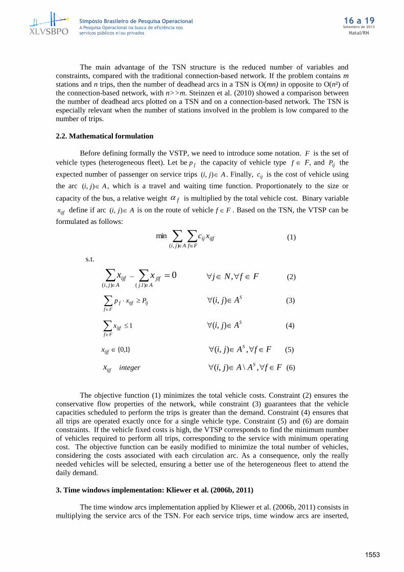
2.2. Mathematical formulation

Before defining formally the VSTP, we need to introduce some notation. F is the set of

vehicle types (heterogeneous fleet). Let be fp the capacity of vehicle type f F, and ijP the

expected number of passenger on service trips Aji ),( . Finally, ijc is the cost of vehicle using

the arc Aji ),( , which is a travel and waiting time function. Proportionately to the size or

capacity of the bus, a relative weight f is multiplied by the total vehicle cost. Binary variable

ijfx define if arc Aji ),( is on the route of vehicle Ff . Based on the TSN, the VTSP can be

formulated as follows:

The objective function (1) minimizes the total vehicle costs. Constraint (2) ensures the

conservative flow properties of the network, while constraint (3) guarantees that the vehicle

capacities scheduled to perform the trips is greater than the demand. Constraint (4) ensures that

all trips are operated exactly once for a single vehicle type. Constraint (5) and (6) are domain

constraints. If the vehicle fixed costs is high, the VTSP corresponds to find the minimum number

of vehicles required to perform all trips, corresponding to the service with minimum operating

cost. The objective function can be easily modified to minimize the total number of vehicles,

considering the costs associated with each circulation arc. As a consequence, only the really

needed vehicles will be selected, ensuring a better use of the heterogeneous fleet to attend the

daily demand.

3. Time windows implementation: Kliewer et al. (2006b, 2011)

The time window arcs implementation applied by Kliewer et al. (2006b, 2011) consists in

multiplying the service arcs of the TSN. For each service trips, time window arcs are inserted,

Aji Ff

ijfij xc

),(

min (1)

s.t.

Aji

ijfx),(

− 0).(

Alj

jlfx FfNj , (2)

Ff

ijijff Pxp SAji ),( (3)

Ff

ijfx 1 SAji ),( (4)

}1,0{ijfx FfAji S ,),( (5)

ijfx integer FfAAji S ,\),( (6)

1553


Natal/RN


each of them represents a trip displacement of a certain amount of time. They assumed discrete

time window values, usually few minutes, to shift some trips of a given timetable and modify

possible departure and arrival times. Fig. 3 shows an example with four service trips and a time

window for each trip of ±2 minutes. By anticipating a trip that starts at 9:20 at Station B for one

or two minutes this trip would be compatible with the trip that starts at 9:54 at Station C.

Figure 3. Arcs Multiplication to consider time window of ± 2 minutes (Kliewer et al., 2006b;

2011)

Station A

Station B

Station C

09:00

09:20

09:25

09:56

09:54

Station A

Station B

Station C

09:00

09:20

09:25

09:56

09:54 Time window arcs

(± 2 minutes)

Station A

Station B

Station C

09:00

09:20

09:25

09:56

09:54

Station A

Station B

Station C

09:00

09:20

09:25

09:56

09:54 Time window arcs

(± 2 minutes)

The insertion of time window arcs leads to a larger mathematical model, generating very

high computational solution times. Because of this, a preprocessing technique was developed to

avoid insertion of a time window arc that does not enable new trip compatibilities compared to

the original service arc. Such unused arcs can be identified from the TSN structure, since only

one arc between all available arcs (service arcs and time window arcs) can be selected. In Fig. 3,

we represent all inserted time window arcs within a defined time interval. In the preprocessing

step, all time window arcs are checked if they enable a new connection from their departure to

their arrival station. If it occurs, the arc is kept on the network, otherwise it is deleted. These

aspects make the computational implementation of time window arcs quite time consuming.

Due to the increasing model complexity, two heuristics were tested to solve the problem

considering the case with multiple depots. The first one, called “trip shortening heuristic” uses a

type of what-if analysis, solving the bus scheduling for the original timetable with equal time

windows for all trips. The solution provides the trips whose shifting lead to additional

connections and in turn reduces the number of necessary vehicles. The resolution for the problem

is obtained from these shifting trips. The second one, “cutting-heuristic”, apply the time-windows

in specific trips, in general, the ones that occur in peaks hours. The second one, “cutting-

heuristic”, is faster than the trip shortening because applies the time-windows just in specific

trips. Compared to the global time windows for all trips of a timetable, which provide the largest

savings but with a long solution time, these heuristics provided compatibles results in a much

shorter time. Concerning the mathematical model each new time window arc requires an

additional flow variable. However, additional constraints are not needed, since the existing cover

1554


Natal/RN


constraints are enhanced by variables corresponding to new arcs. To get a better understanding

about this model, we suggest reading of Kliewer et al. (2006b, 2011).

4. The new time window approach

This section describes in details the time window approach developed towards enhancing

the efficiency of the method, making it possible to apply for a heterogeneous fleet context. The

basic idea of our approach is to add time window arcs linking two trips from the same station,

since they are within the defined time window (usually 1 or 2 minutes). The time window arcs

are expressed in the network like “reversed waiting arcs”, i. e., waiting arcs implemented with an

inverse direction.

The procedure to add time window arcs is defined as follows:

for each station find sAtt 10 , , 10 tt (where 0t is an arrival and 1t is a departure)

if )( 01 tt < time window limit

then add to the network a TW arc which starts in 1t and ends in 0t .

Fig. 4 illustrates two situations in which it is possible to use the time windows arcs and

save vehicles, for a two minutes interval.

Figure 4. Network representation for two minutes time windows

09:32

Station A

Station B

Station C

09:04

09:20

09:34 09:56

09:54

09:32

Station A

Station B

Station C

09:04

09:20

09:34 09:56

09:54

09:52

09:52

09:25

09:25

Time window arc

Virtual arc

Waiting arc

09:32

Station A

Station B

Station C

09:04

09:20

09:34 09:56

09:54

09:32

Station A

Station B

Station C

09:04

09:20

09:34 09:56

09:54

09:52

09:52

09:25

09:25

Time window arc

Virtual arc

Waiting arc

Time window arc

Virtual arc

Waiting arc

To allow a consistent and adjusted timetable and avoid the accumulation of successive

delays on the optimal solution, we added to the model of Section 2.2 a constraint (7), which

requires that whenever there is flow in a time window arc, there must be flow in a waiting arc

1555


Natal/RN


that immediately precedes the service trip performed. The size, in time, of each respective

waiting arc should be at least equal to the time window arc. Thus, the new time window

application becomes very similar to Kliewer’s, which may be represented by the “virtual arc” in

Fig. 4. Let TW the set of time window arcs and WA the set of waiting arcs, the constraint (7)

can be represented by:

0 lkfijf xx ,),( TWji FfAljsucceedklWAkl S ,),(),(:),( (7)

Fig. 5 shows a particular case when two consecutive trips are performed and do not has a

waiting arc immediately after the service arc from the time window arc. The proposed

implementation does not consider the flow represented in the time window arcs because if there

is no waiting arc ),( kl successor of a service arc ),( lj , the constraint (7) is reduced to 0ijfx .

However, in practice, the waiting time between two trips is necessary for the entrance and exit of

passengers at stations and/or for the crew to have a rest, which minimizes this drawback.

Figure 5. Network representation without waiting arcs

09:32

Station A

Station B

Station C

09:04

09:20

09:34 09:56

09:54

09:50

09:23

09:32

We applied a penalty costs to each time window arc to ensure that they only take place if

savings are obtained, as well as for minimizing changes to the original timetabling. From the

solution obtained by the time window model, the timetable can be readjusted. Small time

windows intervals enable few changes at the original timetabling, ensuring the service level and

the passengers’ satisfaction.

5. Computational results

In this section, we describe the results of the carried out experiments to compare the two

different time windows approaches. For those tests, we used real-world instances from a public

transit companies located in the south of Brazil, and large random instances generated based on

real instances with 1000 and 1500 trips. In all instances, the heterogeneous fleet is composed by

three different vehicle types as follows: (i) type A, corresponding to an articulated bus, with

capacity for 141 passengers; (ii) type B, the most commonly used type, with capacity for 100

passengers; and type C, a smaller vehicle able to carry up to 83 passengers. We overestimated the

circulation arcs to find the minimal number of vehicles and define the time window arcs cost

twice more expensive than waiting arcs in our approach and twice more expensive than service

arcs in Kliewer’s approach. We can measure different costs for these arcs because they not

interfere directly in the total number of vehicles (which is subject to the circulation arcs), but may

1556


Natal/RN


impact the distribution of vehicle by types. Time windows are considered with ranges of 2

minutes.

Our main objective is comparing the characteristics of both approaches minimizing the

total number of vehicles. All tests were performed on an Intel Core i7-3612QM 2.10GHz and 8

GB RAM running Ubuntu 12.04.2 LTS. We use ILOG CPLEX 12.4 for computing the solutions.

Table 1 shows the characteristics for real and random instances with its respective origin,

the number of trips (#Trips) and the number of stations (#Stations).

Table 1. Instances characteristics

Instances Origin #Trips #Stations

A_r Real 97 21

B_r Real 499 21

C_r Real 532 9

D_r Real 651 17

A_rd Random 1000 21

B_rd Random 1500 21

Table 2 compares the results for these instances without time windows and with time

windows applying the new (N) and Kliewer’s (K) approaches. We registered the number of

vehicles by type, the total number of vehicles and the solution times in seconds.

Table 2. Comparison of solution approaches to two minutes time windows

type A type B type C

without time window 4 10 35 49 0,02

N 4 10 34 48 0,02

K 4 9 35 48 0,02


N 4 10 34 48 0,16

K 4 9 35 48 0,19


N 1 1 43 45 0,18

K 1 1 43 45 0,19


N 4 10 45 59 0,47

K 4 10 45 59 0,33


N 46 19 129 194 0,82

K 47 20 127 194 0,77


N 50 34 184 268 0,90

K 50 35 183 268 2,20

#Solution

time (sec.)

#vehicles #total

vehicles

A_r

Instance Model type

B_r

C_r

D_r

A_rd

B_rd

Performing a comprehensive analysis, it is clear that the use of TW arcs lead to savings

in the number of scheduled vehicles. Since a very short time window interval was used, the

current timetable was slightly modified, minimally changing the passenger’s routines.

Concerning the objective of this paper, the results indicate that both time window approaches (N

and K) are equivalents, changing (for some instances) only the distribution of vehicles by type.

1557


Natal/RN


We obtained the same vehicle savings for all instances, with low computational cost for both

approaches. These results confirm the practical applicability of the new approach.

Table 3 analyzes the number of service arcs generated in the TSN to solve the model of

the problem, the total number of nodes and arcs generated in both approaches. Table 4 shows the

proportional network reduction in service arcs, nodes and total arcs for the new approach if

compared with Kliewer’s (K / N).

Table 3. Comparison of network size for two minutes time windows

Instance Model type #Service arcs #Nodes #Arcs

without time window 97 178 596

N 97 178 646

K 145 227 775


N 499 1063 3809

K 762 1361 4637


N 532 1133 4044

K 813 1456 4944


N 651 1360 5401

K 989 1730 6506


N 1000 2281 13197

K 1127 2429 13561


N 1500 3385 20140

K 1862 3786 21527

A_r

B_r

C_r

D_r

A_rd

B_rd

Table 4. Network reduction with the new approach

Service

arcsNodes Arcs

A_r 49,5% 27,5% 20,0%

B_r 52,7% 28,0% 21,7%

C_r 52,8% 28,5% 22,3%

D_r 51,9% 27,2% 20,5%

A_rd 12,7% 6,5% 2,8%

B_rd 24,1% 11,8% 6,9%

Reduction

Instance

The network of the developed approach (N) is smaller than the original approach (K),

configured as an alternative proposal to solve problems with a large number of variables and

constraints. With the new approach we can reduce up to 52% the number of service arcs for some

instances, since we do not need perform the multiplication of service arcs to generate the time

window arcs.

6. Conclusions

In this paper, we consider a new mathematical formulation to insert time window

constraints to the vehicle-type scheduling problem. The approach is based on a time-space

1558


Natal/RN


network representation and considers the passengers demand for the fleet scheduling. This is

another differential of the new model, using the demand as a parameter to solve the problem, a

factor often overlooked in the public transportation optimization literature.

The new time window approach is based on the implementation suggested by Kliewer et

al. (2006b, 2011), with some differences: our computational implementation do not need

preprocessing to delete unused time-window arcs and time window arcs are generated in a

similar way to the waiting arcs, instead of multiplying the original service arcs. As a result, a

smaller size network is generated. As shown in Table 2, both approaches are equivalent in terms

of computation time and solution. However, by having a smaller number of nodes and arcs, the

new approach facilitates problem solutions with a large number of variables and constraints.

We intend to apply this new time window approach in order to solve multiple-depot

problems and the integrated vehicle and crew scheduling, considering heterogeneous fleet.

References

Bunte, S. and Kliewer, N. (2009), An overview on vehicle scheduling models in public

transport, Public Transport, 1:4, 299-317.

Carpaneto G., Dell’amico, M., Fischetti, M. and Toth, P. A. (1989), Branch and bound

algorithm for the multiple depot vehicle scheduling problem. Networks, v. 19, p. 531–548.

Ceder, A. (2011) Public-transport vehicle scheduling with multi vehicle type. Transportation

Research Part C, v. 19, p. 485-497.

International Association of Public Transport. (2010). In:

www.globalmasstransit.net/templates/print_preview.html. Accessed in: dec. 2012.

Kliewer, N., Mellouli, T. and Suhl, L. (2002), A new solution model for multi-depot multi-

vehicle-type vehicle scheduling in suburban public transport. In: Mini-EURO Conference and the

EUROWoring Group on Transportation, 2002. Bari, Italy. Proceedings of the 13th Mini-EURO

Conference and the 9thMeeting of the EUROWoring Group on Transportation, Bari.

Kliewer, N., Amberg, B. and Amberg, B. (2011), Multiple depot vehicle and crew scheduling

with time windows for scheduled trips, Public Transport, 3:3, 213-244.

Kliewer, N., Bunte, S. and Suhl, L. (2006b), Time windows for scheduled trips in multiple

depot vehicle scheduling, Proceedings of the EURO Working Group on Transportation, 340-346.

Kliewer, N., Mellouli, T. and Suhl, L. (2002), A new solution model for multi-depot multi-

vehicle-type vehicle scheduling in suburban public transport, Mini-EURO Conference and the

EUROWoring Group on Transportation, 604-609.

Kliewer, N., Mellouli, T. and Suhl, L. (2006a), A TSN based exact optimization model for

multi-depot bus scheduling, European Journal of Operational Research, 175:3, 1616–1627.

Metro Magazine. (2012). METRO’s Top 100 Transit Bus Fleets Survey. In: http://www.metro-

magazine.com/resources/whitepaper/top100.pdf. Accessed in: dec. 2012.

Prefeitura de São Paulo. (2010). Ata da 4ª Reunião do Comitê Municipal de Mudanças do

Clima e Ecoeconomia. São Paulo.

Steinzen, I., Gintner, V and Suhl, L. (2010), A Time-Space Network Approach for the

Integrated Vehicle- and Crew-Scheduling Problem with Multiple Depots, Transportation

Science, 44: 3, 367–382.

van den Heuvel, A. P. R. V. D., van den Akker, J. M. V. D. and Niekerk, M. E. V. K. (2008),

Integrating timetabling and vehicle scheduling in public bus transportation. Technical Report.

Department of Information and Computing Sciences, Utrecht University, Utrecht, The

Netherlands, (http://www.computerscience.nl/research/techreps/repo/CS-2008/2008-003.pdf),

2008.

1559

http://www.globalmasstransit.net/templates/print_preview.html

http://www.metro-magazine.com/resources/whitepaper/top100.pdf

http://www.metro-magazine.com/resources/whitepaper/top100.pdf

http://www.computerscience.nl/research/techreps/repo/CS-2008/2008-003.pdf

a new implementation to the vehicle type scheduling ... · vehicle-type scheduling problem (vtsp)....

Documents