arX

iv:1

307.

2985

v1 [

phys

ics.

chem

-ph]

11

Jul 2

013

A new DFT method for atoms and molecules in Cartesian grid

Amlan K. Roy∗

Division of Chemical Sciences, Indian Institute of Science

Education and Research (IISER), Salt Lake, Kolkata-700106, India

Abstract

Electronic structure calculation of atoms and molecules, in the past few decades has largely been

dominated by density functional methods. This is primarily due to the fact that this can account

for electron correlation effects in a rigorous, tractable manner keeping the computational cost at

a manageable level. With recent advances in methodological development, algorithmic progress

as well as computer technology, larger physical, chemical and biological systems are amenable to

quantum mechanical calculations than ever before. Here we report the development of a new

method for accurate reliable description of atoms, molecules within the Hohenberg-Kohn-Sham

density functional theory (DFT). In a Cartesian grid, atom-centered localized basis set, electron

density, molecular orbitals, two-body potentials are directly built on the grid. We employ a Fourier

convolution method for classical Coulomb potentials by making an Ewald-type decomposition

technique in terms of short- and long-range interactions. One-body matrix elements are obtained

from standard recursion algorithms while two-body counterparts are done by direct numerical

integration. A systematic analysis of our results obtained on various properties, such as component

energy, total energy, ionization energy, potential energy curve, atomization energy, etc., clearly

demonstrates that the method is capable of producing quite accurate and competitive (with those

from other methods in the literature) results. In brief, a new variational DFT method is presented

for atoms and molecules, completely in Cartesian grid.

∗Electronic address: akroy@iiserkol.ac.in, akroy@chem.ucla.edu

1

I. INTRODUCTION

Calculation of wave functions of large molecules by first principles methods has been an

outstanding problem having much relevance in varied fields such as theoretical chemistry,

condensed matter physics, material science, etc. On the one hand, there are standard

Roothaan-Hartree-Fock (RHF)-type methods, as implemented in several quantum chemistry

program packages, though not difficult are certainly tedious and cumbersome indeed, if the

number of basis functions becomes large (which is easily the case for even reasonably smaller

molecules). Also these methods ignore the important effects arising from electron correlation.

On the other side, there are numerous semi-empirical methods, which admittedly have often

found various successful applications in describing molecular properties, but raises many

questions regarding their applicability for some systems such as transition metal complexes

with different kind of ligands. They suffer from the well-known problem of parametrization;

stated differently, a certain parametrization scheme is usually successful for a restricted class

of compounds with respect to a restricted number of properties.

Over the last three decades, there has been considerable progress in the formulation and

implementation of density functional methods, of which Xα or Hartree-Fock-Slater, is the

simplest, best known. The primary reason for this is because it can account for electron

correlation effects in a rigorous, quantitative, transparent manner. Moreover it also provides

a good compromise between computational cost and accuracy. Some other popular routes

toward introducing electron correlation in a many-electron problem are through Moller-

Plesset (MPn) and coupled cluster methods. Density functional theory (DFT) [1–15], in

particular, has become a powerful and versatile tool in recent years; and more preferable

to the other correlated methods, partly because of its favorable scaling (which is typically

N3, although recently linear-scaling methods have been available). Obviously, the ultimate

goal is to be able to describe structure, dynamics, properties of larger and larger systems as

accurately as possible (close to experimental results) with optimal computational resources.

Recent dramatic explosion in computer technology and emergence of accurate density func-

tional techniques, in both formalism and algorithmic aspects, have made it possible to reach

this goal which has eluded quantum chemistry for long. In more practical terms, this is

achieved through a successful marriage of basis-set approaches to electronic structure the-

ory and efficient grid-based quadrature schemes to produce a scaling which is at least as

2

good as self-consistent methods. This also simultaneously allows the very difficult many-

body effects to be approximated by an effective one-electron potential. A proliferation of

DFT-based methodologies has been witnessed for electronic structure calculation of a broad

range of systems including atoms, molecules, clusters, solids and this continues to grow at a

rapid pace.

The key concept of DFT is that all desired properties of a many-electron interacting

system can be obtained in terms of the ground-state electron density, ρ(r), in stead of

a complicated many-electron wave function, as in traditional ab-initio approaches. This

real, non-negative, 3D, scalar function of position is easily visualizable (in contrast to the

wave function which is, in general, complex, 4N dimensional and not so easily interpretable

visually). It has direct physical significance (can be directly measured experimentally) and,

in principle, provides all the informations about ground and all excited states, as obtainable

from a wave function. Initial attempts to use electron density as a basic variable for a

many-electron system, is almost as old as quantum mechanics and is due, independently

to, Thomas and Fermi [16, 17]. In this quantum statistical model, kinetic energy of an

interacting system is approximated as an explicit functional of density (by assuming electrons

to be in the background of a non-interacting homogeneous electron gas), while electron-

nuclear attraction and electron repulsion contributions are treated classically. However,

since this completely ignores the important exchange, correlation effects and kinetic energy

is approximated very crudely, results obtained from this method are rather too crude to

be of any use. It also fails to explain the essential physics and chemistry such as shell

structure of atoms and molecular binding. Significant improvements were made by Dirac [18]

by introducing exchange effects into the picture, the so-called local density approximation

(LDA).

The stark simplicity of these above procedures encouraged multitude of solid-state and

molecular calculations. However, due to a lack of rigorous foundation as well as consider-

ably large errors encountered in these works, the theory lost its charm and appeal until a

breakthrough work by Hohenberg and Kohn [19], which rekindled the hope. This changed

the status of DFT as it got a firm footing and laid the groundwork of all of today’s DFT.

The first theorem simply states that the external potential vext(r), and hence total energy

of an interacting system is a unique functional of ρ(r). According to the second theorem,

ground-state energy can be obtained variationally, i.e., the density that minimizes total en-

3

ergy is the exact ground-state density. Note that although these theorems are very powerful,

they merely prove the existence of a functional, but do not offer any route of computing

this density in practical terms. Even though a mapping between ground-state density and

energy is established, it remains mute about the construction of this “universal” functional.

Thus as far as computational DFT is concerned very little progress is made compared to the

prevailing situation. One still needs to solve the many-body problem in presence of vext(r).

The situation changed dramatically in following year after the publication of a semi-

nal work by Kohn and Sham [20], who proposed a clever route to approach the unknown

universal functional. This is done by mapping the full interacting system of interest with

the real potential onto a fictitious, non-interacting system of particles. The electrons move

in an effective Kohn-Sham (KS) single-particle potential vKS(r) and the auxiliary system

yields same ground-state density as the real interacting system, but greatly simplifies our

calculation. Since exact wave functions of non-interacting fermions are represented by Slater

determinants, major portion of kinetic energy can be computed to a good accuracy, in terms

of one-electron orbitals which construct the reference system. The residual unknown con-

tribution of kinetic energy (which is a fairly small quantity) is dumped in to the unknown,

non-classical component of electron-electron repulsion as,

F [ρ] = Ts[ρ] + J [ρ] + Exc[ρ]

Exc[ρ] = (T [ρ]− Ts[ρ]) + (Eee[ρ]− J [ρ]) = Tc[ρ] + Enc[ρ]. (1)

Ts[ρ] signifies exact kinetic energy of the hypothetical non-interacting system; J [ρ] the clas-

sical component of electron-electron repulsion. In this partitioning scheme then, Exc[ρ] con-

tains everything that is unknown, i.e., non-classical electrostatic effects of electron-electron

repulsion as well as the difference between true kinetic energy Tc[ρ] and Ts[ρ]. Now one can

write the single-particle KS equation in standard form,

[

−1

2∇2 + veff (r)

]

ψi(r) = ǫiψi(r) (2)

with the “effective” potential veff (r) including following terms,

veff (r) = vext(r) +∫

ρ(r′)

|r− r′|dr′ + vxc(r) (3)

where veff (r) and vext(r) signify the effective and external potentials respectively. Exact form

of exchange-correlation (XC) functional remains unknown as yet and its accurate form is

4

necessary for description of real interacting systems (such as binding properties). Numerous

approximations have been suggested for this and development of improved functionals has

constituted one of the most fertile areas of research for several years and even today.

For practical purposes, minimization of the explicit functional is not an easy or efficient

task; and hence not recommended. A far more attractive route is, in stead of working solely

in terms of density, one might bring back the usual orbital picture in to the problem. This

gives an appearance like a single-particle theory, albeit incorporating the many-body effects,

in principle, exactly. In straightforward real-space [21–33] solution of this equation, the wave

functions are sampled on a real grid through either of the following three representations

such as finite difference (FD), finite element (FE) or wavelets where the solution is obtained

in an iterative mechanism. The advantage is that, in all cases, relevant discrete differential

equations offer highly structured, banded sparse matrices. Moreover, the potential operator

is diagonal in coordinate space; Laplacian operator is nearly local (making them ideal candi-

dates for linear-scaling approaches), and these are easily amenable to domain-decomposition

parallel implementation. One can use adaptive mesh refinements or coordinate transforma-

tions to gain further resolution in local regions of space. The whole molecular grid belongs to

either uniform [30, 34, 35] or refined uniform grids [23–26, 29, 32, 33]. The classical electro-

static potential can be found using highly optimized FFTs or real-space multigrid algorithms.

Using FD and FE approach, reasonably successful, fully numerically converged solution for

self-consistent KS eigenvalue problem of atoms/molecules has been reported in literature

[21–23]. In another development, an atom-centered numerical grid [22] was proposed for

performing molecular-orbital (MO) calculation. The physical domain was partitioned into

a collection of single-center components with radial grids centered at each nucleus. Later,

a high-order real-space pseudopotential method [34, 35] was presented for relatively larger

systems in uniform Cartesian coordinates. In an orthogonal 3D mesh, an mth order FD

expansion of the Laplacian can be written as,[

∂2ψ

∂x2

]

xi,yj ,zk

=m∑

−m

Cmψ(xi +mh, yj, zk) +O(h2m+2). (4)

The Hartree potential is obtained by a direct summation on grid by an iterative summation

technique. FD method has been used in different flavors [27, 28, 31, 34, 35] for a number

of interesting ab initio self-consistent problems in clusters and other finite systems, such

as forces, molecular dynamics simulations, polarizabilities of semiconductor clusters as well

5

for areas outside traditional electronic structures. Multigrid methods [32, 36, 37], which

accelerate the self-consistent procedure by reducing number of grid points considerably, have

found many applications in calculations for molecules and large condensed phase systems

on uniform grids. Use of these in conjunction with adaptive grid to enhance the resolution

[27, 38] has been studied. Convergence is influenced by parameters like grid spacing, domain

size, order of representation, etc.

Some of the shortcomings of above approaches are that these are non-variational and

dimension of the Hamiltonian matrix is unmanageably large. In an alternative approach,

finite expansion bases of localized one-electron functions is employed, such as exponential

functions (STO), Gaussian type orbitals (GTO), plane waves (PW), wavelets, numerical

basis sets, linear muffin-tin orbitals, delta functions or some suitable combinations of these.

With STOs or other numerical orbitals, relevant multicenter integrals in the Hamiltonian

needs to be evaluated numerically, while with a Gaussian basis, these and all other integrals

required to compute the matrix elements of Hamiltonian, can be obtained analytically. One

pays a price for using the latter; for considerably larger number of such functions are required

for accurate description of electronic states, as they do not exhibit correct behavior at either

small or large distances from nuclei. Gaussian bases have been extensively used in quantum

chemistry calculations of small and medium molecules, whereas PWs (frequently coupled

with pseudopotentials to treat core electrons) have been most successful for solids. PWs

share with Gaussians the same property that the integrals are known analytically. However,

unlike Gaussians, Coulomb interaction is local in Fourier space—hence solving Poisson’s

equation, a very important step in any DFT calculation, is quite trivial in a PW basis. The

two notable disadvantages of PW bases are: (i) periodic boundary conditions must be used,

which is desirable for solids, but not so in case of clusters or molecules (ii) resolution of

the basis is exactly same everywhere. Thus for atoms and molecules Gaussian bases have

been most successful and popular. Combination of GTO and PW bases have also been used

[39, 40], whereby KS MOs are expanded in Gaussian bases and the electron density in an

augmented PW basis.

Most of the modern DFT programs, for routine calculations, typically employ the so-

called atom-centered grid (ACG), pioneered by Becke [41], where a molecular grid is effi-

ciently described in terms of some suitable 3D numerical quadratures. This is not necessarily

the best strategy, but is a relatively simpler well-defined path, adopted by majority of DFT

6

programs. The basic step consists of partitioning a molecular integral into single-center

discrete overlapping atomic components. For an arbitrary integrand F (r), such a decompo-

sition provides the value of integral I as,

I =∫

F (r)dr =M∑

A

IA, for M nuclei (5)

such that the atomic integrand FA, when summed over all nuclei, returns our original func-

tion. Single-center atomic contributions are denoted by IA =∫

FA(r) dr.

M∑

A

FA(r) = F (r). (6)

FA(r)s are typically constructed from original integrand by some well-behaved weight func-

tions FA(r) = wAF (r). The atomic grid constitutes of a tensor product between radial

part defined in terms of some quadrature formulas such as Gauss-Chebyshev, Gaussian,

Euler-McLaurin, multi-exponential numerical, etc., [42–49] and Lebedev angular quadra-

tures (order as high as 131 has been reported, although usually much lower orders suffice;

59th order being the one most frequently used) [50–54]. Once FAs are determined, IAs are

computed on grid as follows (in polar coordinates),

IA =∫ ∞

0

∫ π

0

∫ 2π

0FA(r, θ, φ)r

2 sin θ dr dθ dφ ≈P∑

p

wradp

Q∑

q

wangq FA(rp, θq, φq), (7)

where wradp , wang

q signify radial, angular weights respectively with P , Q points (total number

of points being P × Q). Usually angular part is not further split into separate θ, φ contri-

butions as surface integrations on a sphere can be done numerically quite easily accurately

by the help of available highly efficient algorithms. Also angular integration has been found

to be much improved by Lobatto scheme [44]. Many variants of this integration scheme

have been proposed thereafter, mainly to prune away any extraneous grid points, which is

much desirable and useful. Integration by dividing whole space and invoking product Gauss

rule [55] has been suggested as well. A variational integration scheme [56] divides molecular

space into three different regions such as atomic spheres, excluded cubic region and inter-

stitial parallelepiped. In a Fourier transform Coulomb and multi-resolution technique, both

Cartesian coordinate grid (CCG) and ACG were used [57–59]; former divides Gaussian shell

pairs into “smooth” and “sharp” categories on the basis of exponents while latter connects

these two by means of a divided-difference polynomial interpolation to translate density and

7

gradients from latter to former. Among other methods, a partitioning scheme [60], linear

scaling [61] and adaptive integration schemes [46, 60, 62] are worth mentioning.

The purpose of this article is to present an alternate DFT method for atoms and molecules

by using a linear combination of GTO expansion for the KS molecular orbitals within CCG

solely [63–65], that has been developed by this author during the past three years. No auxil-

iary basis set is invoked for charge density. Quantities such as localized atom-centered basis

functions, MOs, electron density as well as classical Hartree and non-classical XC potentials

are constructed on the 3D real grid directly. A Fourier convolution method, involving a

combination of FFT and inverse FFT [66, 67] is used to obtain the Coulomb potential quite

accurately and efficiently. Analytical one-electron Hay-Wadt-type effective core potentials

[68, 69], which are made of sum of Gaussian type functions, are used to represent the in-

ner core electrons whereas energy-optimized truncated Gaussian bases are used for valence

electrons. The validity and performance of our method is demonstrated in detail for a mod-

est number of atoms and molecules by presenting total energy, energy components, orbital

energy, potential energy curve, atomization energy for both local [70] and non-local Becke

exchange [71]+Lee-Yang-Parr (LYP) [72] correlation energy functionals. Success of these

above mentioned functionals for various physical, chemical processes are well known. How-

ever, in absence of the exact functional form although these provide very good estimates,

in many occasions they behave rather poorly. Thus construction of more accurate elaborate

sophisticated XC functional lies at the forefront of current research activity as evidenced

by an enormous amount of literature on this. Some frequently used functionals in recent

years are generalized gradient expansion, hybrid, meta or orbital-dependent functionals,

etc. (see, for example, [73], for a brief review). In order to expand the scope, applicability

and feasibility of our method, we have employed two other relatively lesser used functionals

holding good promise, viz., Filatov-Thiel (termed as FT97 in the community) [74, 75] and

PBE [76] functionals, which have been used in many applications with quite decent suc-

cess. Detailed comparisons are made with the widely used GAMESS quantum chemistry

program [77] (grid-based method in ACG and gridless method), and wherever possible, with

experimental results as well. While this work exclusively deals with pseudopotential studies,

full calculations may be investigated in future communications. The article is organized as

follows. Section II gives a brief summary of the methodology. A discussion on our results is

presented in Section IV, while we end with a few concluding remarks in Section V.

8

II. METHODOLOGY AND COMPUTATIONAL CONSIDERATIONS

Details of this method has been published elsewhere [63–65]; here we summarize only

the essential steps. Our starting point is the single-point KS equation for a many-electron

system, which, under the influence of pseudopotentials, can be written as (henceforth atomic

units employed unless otherwise mentioned),[

−1

2∇2 + vpion(r) + vH [ρ](r) + vXC [ρ](r)

]

ψi(r) = ǫiψi(r). (8)

Here vpion denotes the ionic pseudo-potential for the system as,

vpion(r) =∑

Ra

vpion,a(r−Ra) (9)

with vpion,a signifying the ion-core pseudopotential associated with an atom A, situated atRa.

vH [ρ](r) describes the classical Hartree electrostatic interactions among valence electrons,

while vXC [ρ(r)] represents the non-classical XC part of the Hamiltonian, which normally

depends on electron density (and also probably gradient and other derivatives), but not

on wave functions explicitly. {ψσi (r)}, σ = α or β, corresponds to the set of N occupied

orthonormal MOs, to be determined from the solution of this equation.

As already hinted, the so-called, linear combination of atomic orbitals (LCAO) ansatz

is by far, the most popular, convenient and practical route towards an iterative solution of

molecular KS equation. In this scheme, the unknown KS MOs {ψσi (r)}, σ = α, β are linearly

expanded in terms of a set of K known basis functions as,

ψσi (r) =

K∑

µ=1

Cσµiχµ(r), i = 1, 2, · · · , K, (10)

where set {χµ(r)} denotes the contracted Gaussian functions centered on constituent atoms

while {Cσµi} contains contraction coefficients for the orbital ψσ

i (r). The above expression is

exact for a complete set {χµ} with K = ∞ and, in principle, any complete set could be

chosen. However for practical purposes, infinite basis set is not feasible and one is restricted

to a finite set; thus it is of utmost importance to choose suitable basis functions such that

the approximate expansion reproduces unknown KS MOs as accurately as possible. The

procedure is very similar to that applied in HF theory and more practical details could be

found in the elegant books [78–80]. Individual spin-densities are then given by,

ρσ(r) =Nσ∑

i

|ψσi (r)|

2 =Nσ∑

i

K∑

µ=1

K∑

ν=1

CσµiC

σνiχµ(r)χ

∗ν(r) =

∑

µ

∑

ν

P σµνχµ(r)χ

∗ν(r), (11)

9

where P σ stands for the respective density matrices. Denoting the one-electron KS operator

in parentheses of Eq. (5) by fKS, one can write the KS equation in following operator form,

fKSψi(r) = ǫiψi(r). (12)

This operator differs from another similar Fock operator fHF , used in HF theory, in the

sense that former includes all non-classical many-body effects arising from electron-electron

interaction through XC term (as a functional derivative with respect to density, vxc[ρ] =

δExc[ρ]/δρ), whereas there is no provision for such effects in the latter. This represents a

fairly complicated system of coupled integro-differential equation whose numerical solution

is far more demanding and some details are mentioned in the following.

In a spin-unrestricted formalism, substitution of energy terms in to the energy expression,

followed by a minimization with respect to unknown coefficients Cσµi, with ρ(r) = ρα(r) +

ρβ(r) and P = P α + P β, leads to the following matrix KS equation, which is reminiscent of

Pople-Nesbet equation in HF theory,

F αCα = SCαǫα, and F βCβ = SCβǫβ, (13)

with the orthonormality conditions,

(Cα)†SCα = I, and (Cβ)†SCβ = I. (14)

Here Cα, Cβ are matrices containing MO coefficients, S is the atomic overlap matrix, and

ǫα, ǫβ are diagonal matrices of orbital eigenvalues. F α, F β are KS matrices corresponding

to α, β spins respectively, having matrix elements as,

F αµν =

∂EKS

∂P αµν

= Hcoreµν + Jµν + FXCα

µν , and F βµν =

∂EKS

∂P βµν

= Hcoreµν + Jµν + FXCβ

µν . (15)

Here Hcoreµν represents the bare-nucleus Hamiltonian matrix accounting for one-electron ener-

gies including contributions from kinetic energy plus nuclear-electron attraction. Jµν denotes

matrix elements from classical Coulomb repulsion whereas the third term signifies same for

non-classical XC effects. Obviously, this last one constitutes the most difficult and challeng-

ing part of whole SCF process.

At this stage, it is noteworthy that basis-set HF method scales as N4 (total number of

two-electron integrals with N basis functions), while KS calculations do so no worse than N3.

There have been attempts to develop N2 or N logN scaling algorithms by taking into effect

10

the negligible overlap among basis functions involved. In some earlier LCAO-MO-based KS

DFT implementations in GTO bases [81], an auxiliary basis set (in addition to the one used

for MO expansion) was introduced to fit (by some least square or other technique) some

computationally intensive terms to reduce the integral overhead, making it an N3 process.

In one such development [82–84], the electron density and XC potential were expanded in

terms of two auxiliary bases fi, gj respectively as,

ρ(r) ≈ ρ(r) =∑

i

aifi(r) (16)

vxc(r) ≈ vxc(r) =∑

j

bjgj(r).

Here the fitted quantities are identified with tildes while {ai}, {bj}, the fitting coefficients,

are determined by minimization of either a straightforward function of following form,

Z =∫

[ρ(r)− ρ(r)]2dr, (17)

or Coulomb self-repulsion of residual density. Both are subject to the constraint that nor-

malization of fitted density gives total number of electrons. Originally this technique was

first suggested in the context of STOs [85] and later extended to GTOs [82]. Matrix elements

of XC potential (calculated in real-space) were evaluated by some suitable analytical means.

Although this route gained some momentum and was quite successful for many applica-

tions, it suffers from some noteworthy difficulties: (i) many distinct fitting techniques with

varied flavors (variational or non-variational) produce some inconsistency among various

implementations (ii) density and XC fitting constraints differ from method to method (iii)

fitting density does not automatically preserve the conservation of total number of electrons

(iv) such an approach considerably complicates the analytic derivative theories. However,

at the outset, it may be noted that the main reason for such schemes was primarily due

to a lack of efficient method for good-quality multi-center integrals. However, the last few

decades has seen emergence of a huge number of elegant efficient high-quality quadrature

schemes for such integrals offering very accurate results (see, for example, [86], for a lucid

review).

Unlike the exchange integrals in HF theory (which are analytically evaluated within a

GTO basis), KS theory involves far more challenging non-trivial integrals (due to their

complicated algebraic forms). These are not amenable to direct analytic route and resort

must be taken to numerical methods.

11

In this work, the basis functions and MOs are directly built on a real, uniform 3D Carte-

sian grid simulating a cubic box as,

ri = r0 + (i− 1)hr, i = 1, 2, · · · , Nr; for r ∈ {x, y, z}, (18)

where hr, Nr denote the grid spacing and number of grid points respectively (r0 = −Nrhr/2).

The classical electrostatic repulsion as well as XC potentials need to be computed on the

real grid. For finite systems, possibly the simplest and crudest way to compute vH(r) is by

direct numerical integration. This, in general, does not perform efficiently and is feasible

only for relatively smaller systems. The preferred option is to solve the corresponding

Poisson equation. An alternate accurate technique, found to be quite successful in molecular

modeling and used here, involves conventional Fourier convolution method and some variants

[66, 67],

ρ(k) = FFT{ρ(r)} (19)

vH(r) = FFT−1{vcH(k)ρ(k).

Here ρ(k) and vcH(k) represent Fourier integrals of density and Coulomb interaction kernel

respectively in the grid. The former is obtained from a discrete Fourier transform of its

real-space value by standard FFT quite easily. Evaluation of the latter, however, is a non-

trivial task because of the presence of singularity in real space and demands caution. This is

overcome by applying a decomposition of the kernel into long- and short-range interactions,

reminiscent of the commonly used Ewald summation technique in condensed matter physics,

vcH(r) =erf(αr)

r+

erfc(αr)

r≡ vcHlong

(r) + vcHshort(r), (20)

where erf(x) and erfc(x) correspond to error function and its complement respectively. Short-

range Fourier integral can be calculated analytically; the long-range contribution can be

obtained directly from FFT of real-space values. There are several other routes as well

available for classical repulsion as needed in the large-scale electronic structure within KS

DFT framework. More thorough account on this topic can be found in the review [29].

All one-electron contributions of Fock matrix including overlap, kinetic-energy, nuclear-

electron attraction as well pseudopotential matrix elements are completely identical to those

encountered in HF calculation; these are obtained by standard recursion algorithms [87–

89]. Corresponding two-electron matrix elements in real-grid are computed through direct

12

numerical integration in the CCG,

〈φµ(r)|vHXC(r)|φν(r)〉 = hxhyhz∑

grid

φµ(r)vHXC(r)φν(r). (21)

The matrix eigenvalue problem is accurately and efficiently solved using standard LAPACK

routines [90] following usual self-consistent procedure iteratively. The KS eigenfunctions

and eigenvalues then give total energies and/or other quantities in the standard manner.

Convergence of the solution was monitored through (i) potential (ii) total energies and (iii)

eigenvalues. Tolerance of 10−6 a.u., was employed for (ii), (iii), while 10−5 a.u., for (i).

III. RESULTS AND DISCUSSION

Table I, at first, displays various quantities for a representative molecule Cl2, in its ground

state, at an internuclear distance of 4.20 a.u. Non-relativistic energies as well as other

components and total integrated electron density N are given, for LDA XC potential for

different CCG sets, as indicated by grid spacing, hr and number of grid points, Nr (r ∈

x, y, z). Several combinations of grid parameters were tested and finally 8 of them are

presented here, which is sufficient to illustrate the general important features. Most of these

quantities (barring Eh, Ex, Ec) are directly comparable with the commonly used versatile

GAMESS computer program [77] using same basis function, XC potential and effective core

potential. All the LDA calculations referred in this work correspond to the homogeneous

electron-gas correlation of Vosko-Wilk-Nusair (VWN) [70]. The Hay-Wadt valence basis set

employed here, splits valence orbital into inner and outer components described respectively

by two and one primitive Gaussians. Reference values are obtained from two different

options, viz., “grid” and “grid-free” DFT. Former uses the default “army” grade with Euler-

McLaurin quadratures for radial integration and Gauss-Legendre quadrature for angular

integration, while the latter [91, 92] works through a resolution of identity to facilitate

evaluation of relevant molecular integration over functionals rather than quadrature grids.

As the name implies there is no “grid” in the latter and in a sense, it is quite attractive, as

there is no complication that arises from finite grid and associated error. However, there is

a price to pay in the form of an auxiliary basis set to expand the identity which itself suffers

from the same completeness problem. This table illustrates many important points which

are explained in detail in [63]. Here we mention some of the most significant observations.

13

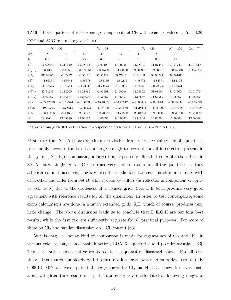
TABLE I: Comparison of various energy components of Cl2 with reference values at R = 4.20.

CCG and ACG results are given in a.u.

Nr = 32 Nr = 64 Nr = 128 Nr = 256 Ref. [77]

Set A B C D E F G H

hr 0.3 0.4 0.2 0.3 0.4 0.1 0.2 0.1

〈T 〉 11.00750 11.17919 11.18733 11.07195 11.06448 11.18701 11.07244 11.07244 11.07320

〈V net 〉 −83.43381 −83.68501 −83.70054 −83.45722 −83.44290 −83.69988 −83.45810 −83.45810 −83.45964

〈Eh〉 37.94086 36.82427 36.83193 36.58714 36.57918 36.83133 36.58747 36.58747

〈Ex〉 −4.86173 −4.86641 −4.86778 −4.84360 −4.84245 −4.86771 −4.84374 −4.84373

〈Ec〉 −0.73575 −0.73521 −0.73530 −0.73374 −0.73366 −0.73530 −0.73374 −0.73374

〈V eet 〉 32.34338 31.22265 31.22885 31.00981 31.00306 31.22832 31.01000 31.01000 31.01078

〈Enu〉 11.66667 11.66667 11.66667 11.66667 11.66667 11.66667 11.66667 11.66667 11.66667

〈V 〉 −39.42376 −40.79570 −40.80503 −40.78074 −40.77317 −40.80489 −40.78144 −40.78144 −40.78219

〈Eel〉 −40.08293 −41.28318 −41.28437 −41.37545 −41.37535 −41.28455 −41.37566 −41.37566 −41.37566

〈E〉 −28.41626 −29.61651 −29.61770 −29.70878 −29.70868 −29.61789 −29.70900 −29.70900 −29.70899a

N 13.89834 13.99939 13.99865 14.00002 14.00003 13.99864 14.00000 13.99999 13.99998

aThis is from grid-DFT calculation; corresponding grid-free DFT value is −29.71530 a.u.

First note that Set A shows maximum deviation from reference values for all quantities

presumably because the box is not large enough to account for all interactions present in

the system. Set B, encompassing a larger box, expectedly offers better results than those in

Set A. Interestingly, Sets B,C,F produce very similar results for all the quantities, as they

all cover same dimensions; however, results for the last two sets match more closely with

each other and differ from Set B, which probably suffers (as reflected in component energies

as well as N) due to the crudeness of a coarser grid. Sets D,E both produce very good

agreement with reference results for all the quantities. In order to test convergence, some

extra calculations are done in a much extended grids G,H, which of course, produces very

little change. The above discussion leads us to conclude that D,E,G,H are our four best

results, while the first two are sufficiently accurate for all practical purposes. For more of

these on Cl2 and similar discussion on HCl, consult [63].

At this stage, a similar kind of comparison is made for eigenvalues of Cl2 and HCl in

various grids keeping same basis function, LDA XC potential and pseudopotentials [63].

These are rather less sensitive compared to the quantities discussed above. For all sets,

these either match completely with literature values or show a maximum deviation of only

0.0001-0.0007 a.u. Next, potential energy curves for Cl2 and HCl are shown for several sets

along with literature results in Fig. I. Total energies are calculated at following ranges of

14

-0.706

-0.705

-0.704

-0.703

-0.702

4 4.1 4.2 4.3 4.4

Ene

rgy

(rel

ativ

e to

-29

a.u

.)

R (a.u.)

Set DSet ESet GSet I

Reference

-0.448

-0.444

-0.44

-0.436

-0.432

2.4 2.6 2.8 3

Ene

rgy

(rel

ativ

e to

-15

a.u

.)

R (a.u.)

Set BSet CSet D

Reference

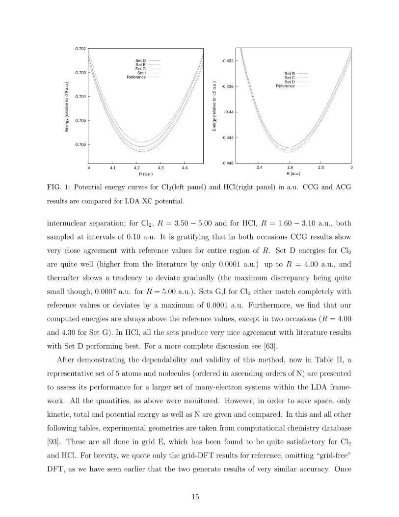
FIG. 1: Potential energy curves for Cl2(left panel) and HCl(right panel) in a.u. CCG and ACG

results are compared for LDA XC potential.

internuclear separation; for Cl2, R = 3.50 − 5.00 and for HCl, R = 1.60 − 3.10 a.u., both

sampled at intervals of 0.10 a.u. It is gratifying that in both occasions CCG results show

very close agreement with reference values for entire region of R. Set D energies for Cl2

are quite well (higher from the literature by only 0.0001 a.u.) up to R = 4.00 a.u., and

thereafter shows a tendency to deviate gradually (the maximum discrepancy being quite

small though; 0.0007 a.u. for R = 5.00 a.u.). Sets G,I for Cl2 either match completely with

reference values or deviates by a maximum of 0.0001 a.u. Furthermore, we find that our

computed energies are always above the reference values, except in two occasions (R = 4.00

and 4.30 for Set G). In HCl, all the sets produce very nice agreement with literature results

with Set D performing best. For a more complete discussion see [63].

After demonstrating the dependability and validity of this method, now in Table II, a

representative set of 5 atoms and molecules (ordered in ascending orders of N) are presented

to assess its performance for a larger set of many-electron systems within the LDA frame-

work. All the quantities, as above were monitored. However, in order to save space, only

kinetic, total and potential energy as well as N are given and compared. In this and all other

following tables, experimental geometries are taken from computational chemistry database

[93]. These are all done in grid E, which has been found to be quite satisfactory for Cl2

and HCl. For brevity, we quote only the grid-DFT results for reference, omitting “grid-free”

DFT, as we have seen earlier that the two generate results of very similar accuracy. Once

15

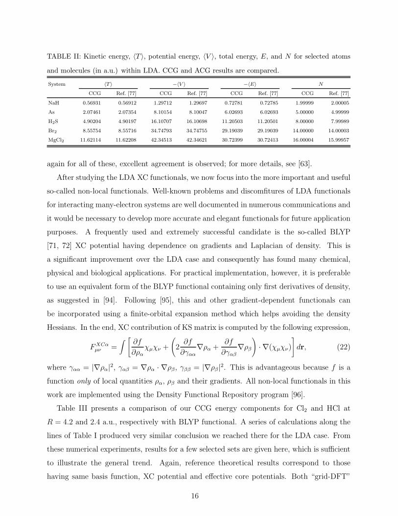
TABLE II: Kinetic energy, 〈T 〉, potential energy, 〈V 〉, total energy, E, and N for selected atoms

and molecules (in a.u.) within LDA. CCG and ACG results are compared.

System 〈T 〉 −〈V 〉 −〈E〉 N

CCG Ref. [77] CCG Ref. [77] CCG Ref. [77] CCG Ref. [77]

NaH 0.56931 0.56912 1.29712 1.29697 0.72781 0.72785 1.99999 2.00005

As 2.07461 2.07354 8.10154 8.10047 6.02693 6.02693 5.00000 4.99999

H2S 4.90204 4.90197 16.10707 16.10698 11.20503 11.20501 8.00000 7.99989

Br2 8.55754 8.55716 34.74793 34.74755 29.19039 29.19039 14.00000 14.00003

MgCl2 11.62114 11.62208 42.34513 42.34621 30.72399 30.72413 16.00004 15.99957

again for all of these, excellent agreement is observed; for more details, see [63].

After studying the LDA XC functionals, we now focus into the more important and useful

so-called non-local functionals. Well-known problems and discomfitures of LDA functionals

for interacting many-electron systems are well documented in numerous communications and

it would be necessary to develop more accurate and elegant functionals for future application

purposes. A frequently used and extremely successful candidate is the so-called BLYP

[71, 72] XC potential having dependence on gradients and Laplacian of density. This is

a significant improvement over the LDA case and consequently has found many chemical,

physical and biological applications. For practical implementation, however, it is preferable

to use an equivalent form of the BLYP functional containing only first derivatives of density,

as suggested in [94]. Following [95], this and other gradient-dependent functionals can

be incorporated using a finite-orbital expansion method which helps avoiding the density

Hessians. In the end, XC contribution of KS matrix is computed by the following expression,

FXCαµν =

∫

[

∂f

∂ραχµχν +

(

2∂f

∂γαα∇ρα +

∂f

∂γαβ∇ρβ

)

· ∇(χµχν)

]

dr, (22)

where γαα = |∇ρα|2, γαβ = ∇ρα · ∇ρβ, γββ = |∇ρβ |

2. This is advantageous because f is a

function only of local quantities ρα, ρβ and their gradients. All non-local functionals in this

work are implemented using the Density Functional Repository program [96].

Table III presents a comparison of our CCG energy components for Cl2 and HCl at

R = 4.2 and 2.4 a.u., respectively with BLYP functional. A series of calculations along the

lines of Table I produced very similar conclusion we reached there for the LDA case. From

these numerical experiments, results for a few selected sets are given here, which is sufficient

to illustrate the general trend. Again, reference theoretical results correspond to those

having same basis function, XC potential and effective core potentials. Both “grid-DFT”

16

TABLE III: Comparison of BLYP energy components for Cl2 and HCl in CCG and ACG, in a.u.

Cl2 (R = 4.2 a.u.) HCl (R = 2.4 a.u.)

Set A B Ref. [77] A B Ref. [77]

Nr 64 128 64 128

hr 0.3 0.2 0.3 0.2

〈T 〉 11.21504 11.21577 11.21570 6.25431 6.25464 6.25458

〈V net 〉 −83.72582 −83.72695 −83.72685 −37.29933 −37.29987 −37.29979

〈Eh〉 36.74464 36.74501 15.86078 15.86103

〈Ex〉 −5.29009 −5.29015 −3.01023 −3.01026

〈Ec〉 −0.37884 −0.37892 −0.21171 −0.21174

〈V eet 〉 31.07572 31.07594 31.07594 12.63884 12.63903 12.63901

〈Enu〉 11.66667 11.66667 11.66667 2.91667 2.91667 2.91667

〈V 〉 −40.98344 −40.98434 −40.98424 −21.74382 −21.74417 −21.74411

〈Eel〉 −41.43506 −41.43524 −41.43522 −18.40618 −18.40620 −18.40620

〈E〉 −29.76840 −29.76857 −29.76855a −15.48951 −15.48953 −15.48953b

N 14.00006 14.00000 13.99998 8.00002 8.00000 8.00000

aThe grid-free DFT value is −29.74755 a.u. [77].bThe grid-free DFT value is −15.48083 a.u. [77].

results in ACG and “grid-free” DFT results for total energy are reported for comparison.

To convince us, some additional reference calculations are performed for a decent number

of atoms/molecules in various extended radial and angular grids besides the default grid of

Nr, Nθ, Nφ = 96, 12, 24, namely, (i) Nr, Nθ, Nφ = 96, 36, 72 (ii) Nr, Nθ, Nφ = 128, 36, 72, with

three integers denoting the number of integration points in r, θ, φ directions respectively.

For the set of species chosen, all these grid sets offer results in very close agreement with

each other. To summarize, out of 17 species, for 8 of them total energies remain unchanged

up to 5th decimal place for all the grids. Very minor variations were observed in remaining

cases (largest deviation in total energy occurs for Na2Cl2, while for all others, it remains

below 0.00007). However, as one passes from default grid to (ii), N gradually improves.

As evident, CCG results are again in perfect agreement with ACG results, as found for the

LDA functional. Obviously Set B produces better results (absolute deviations being 0.00002

and 0.00000 a.u. for Cl2 and HCl respectively) than Set A, but only marginally. Note that

“grid-free” and “grid”-DFT results differ significantly from each other in this case and for

all practical purposes, Set A suffices. Further details can be found in [64].

As in the LDA case, next our calculated BLYP eigenvalues for Cl2 and HCl (at same

R values as in previous tables) are compared in Table IV. Clearly, all the eigenvalues for

17

TABLE IV: Comparison of BLYP negative eigenvalues (in a.u.) of Cl2, HCl with reference values

at R = 4.2 and 2.4. CCG and ACG values are given.

MO Cl2 (R = 4.2 a.u.) MO HCl (R = 2.4 a.u.)

Set A B Ref. [77] A B Ref. [77]

2σg 0.8143 0.8143 0.8143 2σ 0.7707 0.7707 0.7707

2σu 0.7094 0.7094 0.7094 3σ 0.4168 0.4167 0.4167

3σg 0.4170 0.4171 0.4171 1πx 0.2786 0.2786 0.2786

1πxu 0.3405 0.3405 0.3405 1πy 0.2786 0.2786 0.2786

1πyu 0.3405 0.3405 0.3405

1πxg 0.2778 0.2778 0.2778

1πyg 0.2778 0.2778 0.2778

both molecules are very nicely reproduced, as observed for LDA functionals. Excepting the

lone case of 3σ levels (in both cases), where absolute deviation remains only 0.0001 a.u.,

Sets A,B results show a complete matching for all orbital energies. In the same vein of our

LDA approach earlier, we also investigated total energies and other energy components for a

broad range of internuclear distance of Cl2 (R = 3.5− 5.0 a.u) and HCl (R = 1.5− 3.0 a.u.)

both with 0.1 a.u. interval for BLYP XC functional. It is very satisfying that for both of

them, Sets A,B practically coincide with the reference values for the entire range of R. For

Cl2, maximum absolute deviations of 0.0001 and 0.0002 a.u. have been recorded from Sets

B,A respectively. For HCl, the same remains well below 0.0001 a.u. only. A more thorough

discussion is given in [64].

Now Table V compares various energy components (only the kinetic, potential and total

energies) for a few selected atoms and molecules with BLYP XC functional (ordered in

increasing N as we descend the table). A smaller grid of Nr = 64, hr = 0.4 was sufficient

for atoms, whereas a larger grid Nr = 128, hr = 0.3 was used for molecules. Other energy

components are omitted for brevity, as they show very similar agreements with literature

values as observed in previous occasions. The overall agreement for these with reference

values is excellent. For a set of 5 atoms and 10 molecules, total energies are found to be

identical to those from reference values in 5 occasions; otherwise, the maximum absolute

deviation remains below 0.0013%. Results for more atoms and molecules as well as further

observations on this can be found in [64].

Finally, Table VI presents the HOMO energies, −ǫHOMO and atomization energies for

selected 7 molecules in LDA and BLYP approximation, at their experimental geometries

18

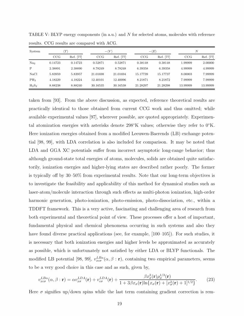
TABLE V: BLYP energy components (in a.u.) and N for selected atoms, molecules with reference

results. CCG results are compared with ACG.

System 〈T 〉 −〈V 〉 −〈E〉 N

CCG Ref. [77] CCG Ref. [77] CCG Ref. [77] CCG Ref. [77]

Na2 0.14723 0.14723 0.52871 0.52871 0.38148 0.38148 1.99999 2.00000

P 2.38891 2.38890 8.78249 8.78248 6.39358 6.39358 4.99999 4.99999

NaCl 5.83959 5.83957 21.01698 21.01694 15.17739 15.17737 8.00003 7.99999

PH3 4.18229 4.18224 12.40101 12.40096 8.21871 8.21872 7.99999 7.99999

H2S2 8.88238 8.88240 30.16535 30.16538 21.28297 21.28298 13.99999 13.99999

taken from [93]. From the above discussion, as expected, reference theoretical results are

practically identical to those obtained from current CCG work and thus omitted; while

available experimental values [97], wherever possible, are quoted appropriately. Experimen-

tal atomization energies with asterisks denote 298◦K values; otherwise they refer to 0◦K.

Here ionization energies obtained from a modified Leeuwen-Baerends (LB) exchange poten-

tial [98, 99], with LDA correlation is also included for comparison. It may be noted that

LDA and GGA XC potentials suffer from incorrect asymptotic long-range behavior; thus

although ground-state total energies of atoms, molecules, solids are obtained quite satisfac-

torily, ionization energies and higher-lying states are described rather poorly. The former

is typically off by 30–50% from experimental results. Note that our long-term objectives is

to investigate the feasibility and applicability of this method for dynamical studies such as

laser-atom/molecule interaction through such effects as multi-photon ionization, high-order

harmonic generation, photo-ionization, photo-emission, photo-dissociation, etc., within a

TDDFT framework. This is a very active, fascinating and challenging area of research from

both experimental and theoretical point of view. These processes offer a host of important,

fundamental physical and chemical phenomena occurring in such systems and also they

have found diverse practical applications (see, for example, [100–105]). For such studies, it

is necessary that both ionization energies and higher levels be approximated as accurately

as possible, which is unfortunately not satisfied by either LDA or BLYP functionals. The

modified LB potential [98, 99], vLBαxcσ (α, β : r), containing two empirical parameters, seems

to be a very good choice in this case and as such, given by,

vLBαxcσ (α, β : r) = αvLDA

xσ (r) + vLDAcσ (r) +

βx2σ(r)ρ1/3σ (r)

1 + 3βxσ(r)ln{xσ(r) + [x2σ(r) + 1]1/2}. (23)

Here σ signifies up/down spins while the last term containing gradient correction is rem-

19

TABLE VI: Comparison of negative HOMO energies, −ǫHOMO (in a.u.) and atomization energies

(kcals/mol) for selected molecules with LDA, LBVWN (LB+VWN) and BLYP XC functionals.

Experimental results [97] are also given, wherever possible. An asterisk indicates 298◦K values.

All others correspond to 0◦K.

Molecule −ǫHOMO (a.u.) Atomization energy (kcals/mol)

LDA BLYP LBVWN Expt. [97] LDA BLYP Expt. [97]

NaBr 0.1818 0.1729 0.3057 0.3050 87.47 78.94 86.8*

SiH4 0.3188 0.3156 0.4624 0.4042 339.43 312.02 302.6

S2 0.2007 0.2023 0.3443 0.3438 56.75 52.47 100.8

BrCl 0.2623 0.2537 0.4133 0.4079 44.95 25.41 51.5

AlCl3 0.3081 0.2976 0.4603 0.4414 278.02 232.88 303.4

P4 0.2712 0.2575 0.3964 0.3432 200.77 142.99 285.9

PCl5 0.2825 0.2722 0.4397 0.3748 246.22 145.33 303.2

iniscent of the exchange functional of [71]. xσ(r) = |∇ρσ(r)|[ρσ(r)]−4/3 is a dimensionless

quantity, α = 1.19, β = 0.01. In this approximation of exchange, asymptotic long-range

property is satisfied properly, i.e., vLBαxcσ (r) → −1/r, r → ∞. Ionization energies obtained

from LBVWN (LB exchange+VWN correlation), reported in Column 4, demonstrates its

superiority over both LDA and BLYP functionals quite convincingly. LDA values are con-

sistently lower than the corresponding BLYP values while LBVWN energies are lower and

more closer to experimental values than both of these. Now calculated atomization energies

in columns 6,7 show significant deviations from experimental results. In several occasions,

surprisingly LDA atomization energies are better than their BLYP counterparts. However,

this should not be used to conclude the superiority of former over the latter, because there

may be some cancellation of errors and also other factors such as more accurate basis func-

tions, core potentials, etc., should be taken in to consideration. Such deviations are not

uncommon in DFT, though. Even very elaborate extended basis set all-electron calcula-

tions on several molecules show very large errors in a recent work [106]. However this is an

on-going activity and does not directly interfere with the main objective of this work.

IV. CONCLUDING REMARKS

We presented an alternate route for atomic/molecular calculation using CCG, within

the framework of GTO-based LCAO-MO approach to DFT. Although several attempts in

20

real-space are known which use CCG, however, to my knowledge, this is the first time such

studies are made in a basis-set approach, solely in CCG. Accuracy and reliability of our

method is illustrated for a cross-section of atoms/molecules through a number of quantities

such as energy components, potential energy curve, atomization energy, ionization potential,

eigenvalue, etc. For a large number of species, these results virtually coincide with those

obtained from other grid-based or grid-free DFT methods available. The success of this

approach lies in an accurate and efficient treatment of the Hartree potential, computed by

a Fourier convolution technique by partitioning the interaction in to long-range and short-

range components. No auxiliary basis set is invoked in to the picture. Detailed comparisons

have been made which shows that the present results are variationally bounded.

V. ACKNOWLEDGMENTS

I thank professors D. Neuhauser, S. I. Chu, E. Proynov for useful discussions.

[1] R. G. Parr and W. Yang. Density Functional Theory of Atoms and Molecules. Oxford

university Press, New York, 1989.

[2] R. O. Jones and O. Gunnarsson. Rev. Mod. Phys., 61:689, 1989.

[3] R. M. Dreizler and E. K. U. Gross (Eds). Density Functional Theory: An Approach to the

Quantum Many-Body Problem. Springer-Verlag, Berlin, 1990.

[4] D. P. Chong (Eds). Recent Advances in Density Functional Methods. World Scientific,

Singapore, 1995.

[5] J. M. Seminario (Eds). Recent Developments and Applications of modern DFT. Elsevier,

Amsterdam, 1996.

[6] D. Joulbert (Eds). Density Functionals: Theory and Applications. Springer, Berlin, 1998.

[7] J. F. Dobson, G. Vignale, and M. P. Das (Eds). Density FunctionalTheory: Recent Progress

and New Directions. Plenum, New York, 1998.

[8] A. Nagy. Phys. Rep., 1:298, 1998.

[9] W. Kohn. Rev. Mod. Phys., 71:1253, 1999.

[10] W. Koch and M. C. Holthausen. A Chemist’s guide to Density Functional Theory. John

21

Wiley, New York, 2001.

[11] R. G. Parr and K. D. Sen. Reviews of Modern Quantum Chemistry: A Celebration of the

Contributions of Robert G. Parr. World Scientific, Singapore, 2002.

[12] C. Fiolhais, F. Nogueira, and M. Marques. A Primer in Density Functional Theory. Springer,

Berlin, 2003.

[13] N. I. Gidopoulos and S. Wilson. The Fundamentals of Electron Density, Density Matrix and

Density Functional Theory in Atoms, Molecules and the Solid State. Springer, Berlin, 2003.

[14] R. M. Martin. Electronic Structure: Basic Theory and Practical Methods. Cambridge Uni-

versity Press, Cambridge, 2004.

[15] D. S. Sholl and J. A. Steckel. Density functional Theory: A Practical Introduction. John-

Wiley, Hoboken, NJ, 2009.

[16] L. H. Thomas. Proc. Camb Phil. Soc., 23:542, 1927.

[17] E. Fermi. Rend. Accad. Lincei, 6:602, 1927.

[18] P. A. M. Dirac. Proc. Camb. Phil. Soc., 26:376, 1930.

[19] P. Hohenberg and W. Kohn. Phys. Rev. B, 136:864, 1964.

[20] W. Kohn and L. J. Sham. Phys. Rev., 140:A1133, 1965.

[21] L. Laaksonen, D. Sundholm, and P. Pyykko. Int. J. Quant. Chem., 27:601, 1985.

[22] A. D. Becke. Int. J. Quant. Chem., 23:599, 1989.

[23] S. R. White, J. W. Wilkins, and M. P. Teter. Phys. Rev. B., 39:5819, 1989.

[24] E. Tsuchida and M. Tsukada. Phys. Rev. B, 52:5573, 1995.

[25] T. L. Beck, K. A. Iyer, and M. P. Merrick. Int. J. Quant. Chem., 61:341, 1997.

[26] E. Hernandez, M. J. Gillan, and C. M. Goringe. Phys. Rev. B, 55:13485, 1997.

[27] N. A. Modine, G. Zumbach, and E. Kaxiras. Phys. Rev. B., 55:10289, 1995.

[28] Y.-H. Kim, M. Staedele, and R. M. Martin. Phys. Rev. A., 60:3633, 1999.

[29] T. L. Beck. Rev. Mod. Phys., 72:1041, 2000.

[30] J. R. Chelikowsky, Y. Saad, S. Ogut, I. Vasiliev, and A. Stathopoulos. Phys. Status Solidi

B, 217:173, 2000.

[31] I.-H. Lee, Y.-H. Kim, and R. M. Martin. Phys. Rev. B., 61:4397, 2000.

[32] J. Wang and T. L. Beck. J. Chem. Phys., 112:9223, 2000.

[33] L. Kronik, A. Makmal, M. L. Tiago, M. M. G. Alemany, M. Jain, X. Huang, Y. Saad, and

J. R. Chelikowsky. Phys. Status Solidi B, 243:1063, 2006.

22

[34] J. R. Chelikowsky, R. N. Troullier, and Y. Saad. Phys. Rev. Lett., 72:1240, 1994.

[35] J. R. Chelikowsky, R. N. Troullier, K. Wu, and Y. Saad. Phys. Rev. B., 50:11355, 1994.

[36] E. L. Briggs, D. J. Sullivan, and J. Bernholc. Phys. Rev. B., 52:R5471, 1995.

[37] E. L. Briggs, D. J. Sullivan, and J. Bernholc. Phys. Rev. B., 54:14375, 1996.

[38] F. Gygi and G. Galli. Phys. Rev. B., 52:R2229, 1995.

[39] G. Lippert, J. Hutter, and M. Parinello. Theor. Chem. Acc., 103:124, 1999.

[40] M. Krack and M. Parinello. Phys. Chem. Chem. Phys., 2:2105, 2000.

[41] A. D. Becke. J. Chem. Phys., 88:2547, 1988.

[42] P. M. W. Gill, B. G. Johnson, and J. A. Pople. Chem. Phys. Lett., 209:506, 1993.

[43] C. W. Murray, N. C. Handy, and G. J. Laming. Mol. Phys., 78:997, 1993.

[44] O. Treutler and R. Ahlrichs. J. Chem. Phys., 102:346, 1995.

[45] M. M. Mura and P. J. Knowles. J. Chem. Phys., 104:9898, 1996.

[46] M. Krack and A. M. Koster. J. Chem. Phys., 108:3226, 1998.

[47] R. Lindh, P.-A. Malmqvist, and L. Gagliardi. Theor. Chem. Acc., 106:178, 2001.

[48] P. M. W. Gill and S. H. Chien. J. Comput. Chem., 277:730, 2003.

[49] S. H. Chien and P. M. W. Gill. J. Comput. Chem., 27:730, 2006.

[50] V. I. Lebedev and Zh. Vychisl. Mat. Mat. Fiz., 15:48, 1975.

[51] V. I. Lebedev and Zh. Vychisl. Mat. Mat. Fiz., 16:293, 1976.

[52] V. I. Lebedev and A. L. Skorokhodov. Russ. Acad. Sci. Docl. Math. , 45:587, 1992.

[53] V. I. Lebedev. Dokl. Akad. Nauk, 338:434, 1994.

[54] V. I. Lebedev and D. N. Laikov. Dokl. Akad. Nauk, 366:741, 1999.

[55] P. M. Boerrigter, G. Te. Velde, and E. J. Baerends. Int. J. Quant. Chem., 33:87, 1988.

[56] M. R. Pederson and K. A. Jackson. Phys. Rev. B, 41:7453, 1990.

[57] L. Fusti-Molnar and J. Kong. J. Chem. Phys., 122:74108, 2005.

[58] S. T. Brown, L. Fusti-Molnar, and J. Kong. Chem. Phys. Lett., 418:490, 2006.

[59] J. Kong, S. T. Brown, and L. Fusti-Molnar. J. Chem. Phys., 124:094109, 2006.

[60] H. Ishikawa, K. Yamamoto, K. Fujima, and M. Iwasawa. Int. J. Quant. Chem., 72:509, 1999.

[61] R. E. Stratmann, G. E. Scuseria, and M. J. Frisch. Chem. Phys. Lett., 257:213, 1996.

[62] K. Yamamoto, K. Fujima, and M. Iwasawa. J. Chem. Phys., 108:8769, 1997.

[63] A. K. Roy. Int. J. Quant. Chem., 108:837, 2008.

[64] A. K. Roy. Chem. Phys. Lett., 461:142, 2008.

23

[65] A. K. Roy. In C. T. Collett and C. D. Robson, editors, Handbook of Computational Chemistry

Research, New York, 2009. Nova publishers.

[66] G. C.Martyna and M. E. Tuckerman. J. Chem. Phys., 110:2810, 1999.

[67] P. Minary, M. E. Tuckerman, K. A. Pihakari, and G. J. Martyna. J. Chem. Phys., 116:5351,

2002.

[68] W. R. Wadt and P. J. Hay. J. Chem. Phys., 82:284, 1985.

[69] P. J. Hay and W. R. Wadt. J. Chem. Phys., 82:299, 1985.

[70] S. H. Vosko, L. Wilk, and M. Nusair. Can. J. Phys., 58:1200, 1980.

[71] A. D. Becke. Phys. Rev. A, 38:3098, 1988.

[72] C. Lee, W. Yang, and R. G. Parr. Phys. Rev. B, 37:785, 1988.

[73] C. J. Cramer. Essentials of Computational Chemistry: Theories and Models. John Wiley,

New York, 2004.

[74] M. Filatov and W. Thiel. Mol. Phys., 91:847, 1997.

[75] M. Filatov and W. Thiel. Int. J. Quant. Chem., 62:603, 1997.

[76] J. P. Perdew, K. Burke, and M. Ernzerhof. Phys. Rev. Lett., 77:3865, 1996.

[77] M. W. Schmidt, K. K. Baldridge, J. A. Boatz, S. T. Elbert, M. S. Gordon, J. H. Hensen,

S. Koseki, N. Matsunaga, K. A. Nguyen, S. J. Su, T. L. Windus, M. Dupuis, and J. A.

Montgomery. J. Comput. Chem., 14:1347, 1993.

[78] A. Szabo and N. S. Ostlund. Modern Quantum Chemistry. Dover, New York, 1996.

[79] P. Jorgensen T. Helgaker and J. Olsen. Modern Electronic Structure Theory. John Wiley,

New York, 2000.

[80] F. Jensen. Introduction to Computational Chemistry. John Wiley, New York, 2007.

[81] J. Andzelm and E. Wimmer. J. Chem. Phys., 96:1280, 1992.

[82] H. Sambe and R. H. Felton. J. Chem. Phys., 62:1122, 1975.

[83] B. I. Dunlap, J. W. D. Connolly, and J. R. Sabin. J. Chem. Phys., 62:1122, 1979.

[84] B. I. Dunlap, J. W. D. Connolly, and J. R. Sabin. J. Chem. Phys., 71:3396, 1979.

[85] E. J. Baerends, D. E. Ellis, and P. Ros. Chem. Phys., 2:41, 1973.

[86] P. M. W. Gill. Adv. Quant. Chem., 25:141, 1994.

[87] S. Obara and A. Saika. J. Chem. Phys., 84:3963, 1986.

[88] L. E. McMurchie and E. R. Davidson. J. Chem. Phys., 26:218, 1978.

[89] L. R. Kahn, P. Baybutt, and D. G. Truhlar. J. Chem. Phys., 65:3826, 1976.

24

[90] E. Anderson, Z. Bai, C. Bischof, S. Blackford, J. Demmel, J. Dongarra, J. Du Croz, A. Green-

baum, S. Hammarling, A. McKenney, and D. Sorensen. LAPACK Users’ Guide (3rd Ed.).

SIAM, Philadelphia, 1999.

[91] Y. C. Zheng and J. Almlof. J. Chem. Phys., 214:397, 1993.

[92] K. R. Glaesemann and M. S. Gordon. J. Chem. Phys., 108:9959, 1998.

[93] R. D. Johnson III (Eds.). NIST Computational Chemistry Comparisons and Benchmark

Database, NIST Standard Reference Database, Number, Release 14. NIST, Gaithersburg,

MD, 2006.

[94] B. Miehlich, A. Savin, H. Stoll, and H. Preuss. Chem. Phys. Lett., 157:200, 1989.

[95] J. A. Pople, P. M. W. Gill, and B. G. Johnson. Chem. Phys. Lett., 199:557, 1992.

[96] Quantum Chemistry Group. Density Functional Repository. CCLRC Daresbury Laboratory,

Daresbury, Cheshire, UK.

[97] H. Y. Afeefy, J. E. Liebman, in P. J. Linstrom S. E. Stein, and W. G. Mallard (Eds). NIST

Chemistry Webbook, NIST Standard Reference Database, Number 69. NIST, Gaithersburg,

MD, 2005.

[98] R. van Leeuwen and E. J. Baerends. Phys. Rev. A, 49:2421, 1994.

[99] P. R. T. Schipper, O. V. Gritsenko, S. J. A. van Gisbergen, and E. J. Baerends.

J. Chem. Phys, 112:1344, 2001.

[100] T. Brabec and F. Krausz. Rev. Mod. Phys., 72:545, 2000.

[101] Th. Udem, R. Holzwarth, and T. W. Hansch. Nature (London), 416:233, 2002.

[102] A. Baltuska, Th. Udem, M. Uiberacker, M. Hentschel, E. Goulielmakis, Ch. Gohle,

R. Holzwarth, V. S. Yakolev, A. Scrinzi, T. W. Hansch, and F. Krausz. Nature (London),

421:611, 2003.

[103] H. Stapelfeldt and T. Seideman. Rev. Mod. Phys., 75:543, 2003.

[104] J. H. Posthumus. Rep. Prog. Phys., 67:623, 2004.

[105] Ch. Gohle, Th. Udem, M. Herrmann, J. Rauschenberger, R. Holzwarth, H. A. Schuessler,

F. Krausz, and T. W. Hansch. Nature (London), 436:234, 2005.

[106] M. Cafiero. Chem. Phys. Lett., 418:126, 2006.

25