discovery of a general method of solving the schr€odinger ... · ust as newtonian law governs...
TRANSCRIPT

1480 ’ ACCOUNTS OF CHEMICAL RESEARCH ’ 1480–1490 ’ 2012 ’ Vol. 45, No. 9 Published on the Web 06/11/2012 www.pubs.acs.org/accounts10.1021/ar200340j & 2012 American Chemical Society
Discovery of a General Method of Solving theSchr€odinger and Dirac Equations That Opens a
Way to Accurately Predictive Quantum ChemistryHIROSHI NAKATSUJI*
Quantum Chemistry Research Institute and JST-CREST, Kyodai Katsura VenturePlaza 107, Goryo Oohara 1-36, Nishikyo-ku, Kyoto 615-8245, Japan
RECEIVED ON DECEMBER 30, 2011
CONS P EC TU S
J ust as Newtonian law governs classical physics,the Schr€odinger equation (SE) and the relativistic
Dirac equation (DE) rule the world of chemistry. So, ifwe can solve these equations accurately, wecan use computation to predict chemistry precisely.However, for approximately 80 years after thediscovery of these equations, chemists believed thatthey could not solve SE and DE for atoms andmolecules that included many electrons. This Accountreviews ideas developed over the past decade tofurther the goal of predictive quantum chemistry.
Between 2000 and 2005, I discovered a generalmethod of solving the SE and DE accurately. As a firstinspiration, I formulated the structure of the exactwave function of the SE in a compact mathematicalform. The explicit inclusion of the exact wave func-tion's structure within the variational space allowsfor the calculation of the exact wave function as asolution of the variational method. Although thisprocess sounds almost impossible, it is indeed possible, and I have published several formulations and applied them to solvethe full configuration interaction (CI) with a very small number of variables. However, when I examined analytical solutions foratoms and molecules, the Hamiltonian integrals in their secular equations diverged. This singularity problem occurred in allatoms and molecules because it originates from the singularity of the Coulomb potential in their Hamiltonians. To overcome thisproblem, I first introduced the inverse SE and then the scaled SE. The latter simpler idea led to immediate and surprisinglyaccurate solution for the SEs of the hydrogen atom, helium atom, and hydrogen molecule.
The free complement (FC) method, also called the free iterative CI (free ICI) method, was efficient for solving the SEs. In the FCmethod, the basis functions that span the exact wave function are produced by the Hamiltonian of the system andthe zeroth-order wave function. These basis functions are called complement functions because they are the elements ofthe complete functions for the system under consideration. We extended this idea to solve the relativistic DE and applied it tothe hydrogen and helium atoms, without observing any problems such as variational collapse. Thereafter, we obtained veryaccurate solutions of the SE for the ground and excited states of the Born�Oppenheimer (BO) and non-BO states of very smallsystems like He, H2
þ, H2, and their analogues. For larger systems, however, the overlap and Hamiltonian integrals over thecomplement functions are not always known mathematically (integration difficulty); therefore we formulated the local SE (LSE)method as an integral-free method. Without any integration, the LSE method gave fairly accurate energies and wave functions forsmall atoms and molecules. We also calculated continuous potential curves of the ground and excited states of small diatomicmolecules by introducing the transferable local sampling method. Although the FC-LSE method is simple, the achievement ofchemical accuracy in the absolute energy of larger systems remains time-consuming. The development of more efficient methodsfor the calculations of ordinary molecules would allow researchers to make these calculations more easily.

Vol. 45, No. 9 ’ 2012 ’ 1480–1490 ’ ACCOUNTS OF CHEMICAL RESEARCH ’ 1481
Method of Solving the Schr€odinger and Dirac Equations Nakatsuji
IntroductionThe Schr€odinger equation (SE) and the relativistic Dirac equa-
tion (DE) are thebasic equations that govern theworldof atoms
andmolecules,1 just as theNewton's andEinstein's lawsgovern
the macroscopic and cosmic world.2 In the latter world, the
basic principles are able to provide very accurate predictions
that enable applications such as interplanetary journeys to
occur. However, in the former world, such accurate predictions
are limited only to the hydrogen atom and some simple one-
electron systems. Formany-electron atoms andmolecules that
are daily subjects in chemistry, even modern quantum chem-
istry cannot provide predictions as accurate as those in the
Newtonian world. The reason for this is simple. The basic
equations in classical mechanics can be solved to their intrinsic
accuracies, but in the quantum world, the SE and DE have not
been solved in their limiting accuracies: they are solved only
approximately. People thought formany years, and aftermany
trials, that solving the SE andDEwas essentially impossible. This
was so for about 80 years after the discovery of the SE.
Modernquantumchemistry ismuchdevelopedandprovides
useful tools for understanding1 the underlying nature of chemical
phenomena. However, even the advanced theories encounter
difficulties when applied to bond-fission processes.3 However, if
a general andaccuratemethodof solving the SEandDE is estab-
lished, we will be able to enjoy truly predictive quantum chem-
istry. Someyearsago, theauthordiscoveredageneralmethodof
solving the SE and DE,4�10 and this method is now being devel-
oped in our Institute to realize the above dream. The purpose of
this Account is to provide an expository reviewof the basic ideas
and their applications to calculate the full configuration interac-
tion (CI) andanalytical solutionsof theSEofatomsandmolecules.
Onlyminimumpossible formulas andmathematics will be used.
How Accurate Are the SE and DE?Thehydrogen atom is theonly example forwhich the SE and
DE are exactly solvable. The exact energy of the SE is
E(n) ¼ �μZ2=(2n2) (1)
where Z is the nuclear charge, n is the principal quantum
number, and μ is the reduced mass. Similarly, the exact
energy of the DE is given by11
E(n0, j) ¼ 1ffiffiffiffiffiffiffiffiffiffiffiffiffiffiffiffiffiffiffiffiffiffiffiffiffiffiffiffiffiffiffiffiffiffiffiffiffiffiffiffiffiffiffiffiffiffiffiffiffiffiffiffiffiffiffiffiffiffiffiffi1þ Z2R2
(n0þffiffiffiffiffiffiffiffiffiffiffiffiffiffiffiffiffiffiffiffiffiffiffiffiffiffiffiffiffiffiffiffiffiffiffi(jþ1=2)2 � Z2R2
q)2
vuut� 1
0BBBBBBB@
1CCCCCCCAμ (2)
where n0 is similar to n above, j is the total angular
momentum quantum number, and R = 1/137.03599 is
the fine structure constant. We used the atomic unit in
this Account (for energy, 1 au = 27.21134 eV, 627.5096
kcal/mol, or 219 474.6315 cm�1). For the hydro-
gen atom, the experimental ground-state energy12
is �0.499733191, the SE energy is �0.499 727840,
and the DE energy is �0.499 73449. We can calculate
the excitation energy for the excitation fromn=1 to n=2.
The experimental values are 0.374799317 for 2s(1/2),
0.374799158 for 2p(1/2), and 0.374800821 for 2p(3/2),
where small differences are observed for the 2s and 2p
states. The value in parentheses is the j value. The SE
gives only a single value of 0.374 795880 for these three
different states. TheDEgives a valueof 0.374 800452 for
the 2s(1/2) and 2p(1/2) states and 0.374 802115 for the
2p(3/2) state. The DE cannot explain the small difference
between the 2s(1/2) and 2p(1/2) states. This difference is
called the Lamb shift and is explained by quantum
electrodynamic (QED) theory,11 which is beyond the
scope of the present Account.The reader has no doubt been very impressed with the
high accuracy of the energies predicted by the SE and DE.
The SE predicts the energy to four-digit accuracy and the DE
to five digits. Certainly, the DE gives a higher accuracy than
the SE, but the SE is already highly accurate for the hydrogen
atom. This is true for the first row elements in the Periodic
Table. For heavier elements, the relativistic effects expressed
by the DE become more important. Therefore, if we have a
theory that enables us to solve the SE and DE to a high
accuracy and if we can apply it to atoms and molecules that
appear daily in chemistry, then our science will be highly
elevated to be truly predictive for chemical science. In this
case, computer simulations would become a complemen-
tary methodology that would compete with experiments. Is
this just a dream? Is there anyway to realize this dream?We
are trying to realize this dream.
The Schr€odinger and Dirac EquationsWhat are the SE and DE? They have very simple and similar
forms. The SE is written as
Hψ ¼ Eψ (3)
where the Hamiltonian is given by
H ¼ �Xi
12Δi �
Xi
XA
ZArAi
þXi>j
1rijþ
XA>B
ZAZBRAB
(4)

1482 ’ ACCOUNTS OF CHEMICAL RESEARCH ’ 1480–1490 ’ 2012 ’ Vol. 45, No. 9
Method of Solving the Schr€odinger and Dirac Equations Nakatsuji
in ordinary notation. The SE is a second-order differen-
tial equation. This differential equation can be solved
analytically for the hydrogen atom, as explained above.
However, for more-than-two electron systems, there is no
direct analytical way to solve their differential equations. In
our generalmethodof solving the SE,wedonot try to solve
the “differential” equation. It is noted here that the differ-
entiation is always possible for the analytical functions. In
contrast, integration is not always “possible” for all analy-
tical functions, even though one may know intuitively the
existence of the integral values. It is fortunate that the SE
does not include any integration in its expression.The DE is written similarly to the SE as
HΨ ¼ EΨ (5)
where the Hamiltonian,H, is not a scalar operator but is a
matrix operator with the dimension of N4, with N being
the number of electrons of the system. Similarly, Ψ is a
vector function with the same dimension. This Account is
mainly focused on the SE, so we will not give the explicit
formof theHamiltonian of theDE. However,we note that
what we call DE here is actually the Dirac�Coulomb
equation, which is a generalization of the one-electron
Dirac equation11 to the many-electron case. Because of
the similarity between the SE and DE, the method of
solving the SE can be applied to the DE9 with a small
modification. Finally, we note that we specify the true
solutions of the SE and DE by using the word “exact”.
Variational PrincipleProbably the most frequently used principle in computa-
tional chemistry is the variational principle (VP),
δE[ψ] ¼ 0: (6)
Suppose that we try to solve the SE of a given system.We
use ψ as the candidate for a solution. It includes some
variable parameters within an assumed functional form.
An importantmerit of the VP is that it always provides the
optimal values for such parameters. However, it is sel-
dom to obtain the solution of the SE using this method,
because it is very difficult to predict the exact functional
form of a many-electron system by intuition alone. Even
so, this principle gives us the best possible wave function
within the assumed functional form.If we can prepare a trial function that surely includes the
exact wave function within its functional form, the VP
method gives the exact wave function as its solution.
Most people would probably think that this is not possible.
However, it is both possible and easy, as shown below. We
shall designate such a functional form as having an exact
structure.
Exact StructureInaseriesofpapersstarting from2000, theauthorhaspublished
several ideas under the title of “the structure of the exact wave
function”.4,5,13�15 The details are given in the references, but
what we need here is simple. Let us compare three very
important fundamental formulas. The first is the SE itself,
(H � E)ψ ¼ 0 (7)
which defines the exact wave function and its energy. The
second formula is the VP, which is now written as
ÆψjH � Ejδψæ ¼ 0 (8)
The third formula is what we call an H-square equation,
Æψj(H � E)2jψæ ¼ 0 (9)
The H-square equation is unique in that it is equivalent to
the SE. Only the solution of the SE can satisfy this equation.
The proof is simple and has been given previously.,
Now let us compare eqs 8 and 9. Then, we can easily
reach the following theorem.
Theorem. Letψ be a function that includes a parameter C
and satisfies the relationship
δψ ¼ (H � E)ψ 3δC (10)
Then thisψ has an exact structure, because its variational
solution satisfies the H-square equation and therefore is
exact.Proof. Because δψ is given by eq 10, we can substitute it
into the VP, eq 8, and obtain Æψ|(H � E)2|ψæ 3 δC = 0. Since this
equationmust hold for any δC, we obtain eq 9. Namely, when
ψ satisfies eq 10, its VP solution satisfies theH-square equation
at the same time, and therefore it is exact (end of proof).
Thus, when we prepare our wave function to satisfy
eq 10, its variational solution is guaranteed to be exact. It
is very important to use a wave function that has an exact
structure to formulate the method of solving the SE.
Simplest Iterative Complement MethodWhat ψ satisfies eq 10? There are several possibilities.8
Among these, a simple expression is given by the following
recursion formula:4,5
ψnþ1 ¼ [1þ Cn(H � En)]ψn (11)

Vol. 45, No. 9 ’ 2012 ’ 1480–1490 ’ ACCOUNTS OF CHEMICAL RESEARCH ’ 1483
Method of Solving the Schr€odinger and Dirac Equations Nakatsuji
where n is the iteration number, Cn is one parameter in
each iteration, and En = Æψn|H|ψnæ. Because this is the
simplest form among what we call iterative complement
(IC) methods, we shall denote it as the simplest IC (SIC)
method. It is easy to prove that a SIC wave function
becomes exact at convergence., Applying the variational
principle to eq 11, we obtain a very simple 2 � 2 secular
equation, and by solving it successively, we are able to
obtain an exact solution of the SE at convergence.
Full Configuration InteractionWhenwe solve the SEwithin a given basis set, the solution is
the so-called full CI (configuration interaction). This is usually
obtained after the diagonalization of a very large Hamilto-
nianmatrix,whichmakes thismethoddifficult to perform for
large molecules with a very good basis set.
Insofar as the SIC equation is correct, we should be able to
calculate the full-CI solution using the SIC method starting
fromanapproximate function, suchas theHartree�Fock, forψ0.
This is performed by replacing the Hamiltonian operator in
eq 11 with the Hamiltonian matrix over the full-CI config-
urations. Figure 1 shows the results for several molecules
using minimal basis set.16,17 Certainly, all the calculations
converged to the full-CI energies after the iterations were
performed. For HNCO, the full-CI calculation was per-
formed by the diagonalization of the Hamiltonian matrix
with a dimension of 216 247, while the same result was
obtained using the SICmethod after 68 iterations of a two-
dimensional diagonalization. However, the convergence
rate was very slow by the reason that will be explained
later.18
Singularity ProblemThe full CI is best only within a given basis set. When we
improve the basis set, the dimension of the full CI increases
rapidly and a solution becomes impossible. Therefore, a
better way is to solve the SE analytically. However, whenwe
perform the SIC calculations analytically, we encounter a
significant obstacle that we call the singularity problem.6�8
This is caused by the Coulomb potential that is included in
the Hamiltonians of atoms and molecules. The nuclear�electron attraction potential and the electron�electron re-
pulsion potential become infinite when two particles meet.
For this reason, the integral of the Hamiltonian over an
approximate wave function, ψ~, diverges to plus or minus
infinity when the integerm has a value ofmg 3, as follows.
Æψ~jHmjψ~æ ¼ (¥ (mg3) (12)
The proof is easy, as is shown in Figure 2. The upper part
shows the quantity ψ~*ψ~, which is always finite. The lower
part shows the mth power of the Coulomb potential multi-
plied by the Jacobian with order r2. Near to the origin, the
lower factor becomes minus infinity when m g 3, and
therefore the integral diverges to infinity. This singularity
problem is actually a significant obstacle. For example, in SIC
calculations (eq 11), the nth order function includes the term
Hnψ0. Therefore, the Hamiltonian matrix of this term
FIGURE 1. Convergence process of the SIC calculations to the full-CIenergy using the ordinary Hamiltonian matrix of the minimal STO-6Gbasis. FIGURE 2. Illustrative proof of the singularity of the Hamiltonian
integral expressed by eq 12.
1484 ’ ACCOUNTS OF CHEMICAL RESEARCH ’ 1480–1490 ’ 2012 ’ Vol. 45, No. 9
Method of Solving the Schr€odinger and Dirac Equations Nakatsuji
includes H2nþ1, and so diverges even when n = 1. Therefore,
the analytical calculations break down.
Inverse Schr€odinger EquationThe author proposed two different ways to avoid the singu-
larity problem. The first was to introduce the inverse
Schr€odinger equation (ISE),6
H�1ψ ¼ E�1ψ (13)
where H�1 is the inverse Hamiltonian and E�1 is the
inverse of the energy E. This equation is equivalent to
the original SE6 Even infinite values become zero when
we introduce the inverse Hamiltonian.In the SIC calculations of the full CI shown in Figure 1, we
multiplied the full-CI Hamiltonian matrix many times. This
could be done simply owing to the crudeness of the basis
set: the STO-6G set cannot be a complete set. But, with the
analytic Hamiltonian, this is, in principle, not possible because
of the singularity problem. Therefore, SIC calculations with
ordinary Hamiltonians are problematic, which is a reason for
the slow convergence observed in Figure 1.18 When we take
the inverse of the full-CI Hamiltonian matrix, then it is the
matrix of the inverse Hamiltonian, so what happens when we
performSIC calculationsusing the inverseHamiltonianmatrix?
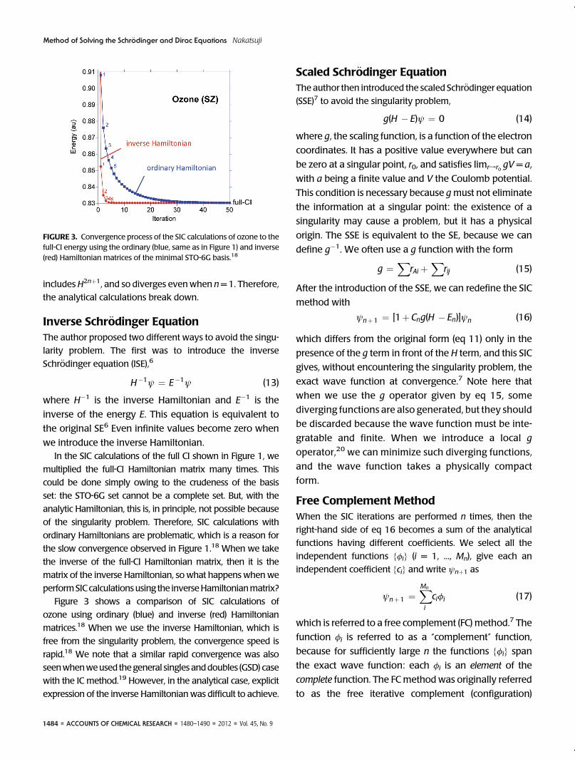
Figure 3 shows a comparison of SIC calculations of
ozone using ordinary (blue) and inverse (red) Hamiltonian
matrices.18 When we use the inverse Hamiltonian, which is
free from the singularity problem, the convergence speed is
rapid.18 We note that a similar rapid convergence was also
seenwhenweused thegeneral singles anddoubles (GSD) case
with the IC method.19 However, in the analytical case, explicit
expression of the inverse Hamiltonian was difficult to achieve.
Scaled Schr€odinger EquationThe author then introduced the scaled Schr€odinger equation
(SSE)7 to avoid the singularity problem,
g(H � E)ψ ¼ 0 (14)
where g, the scaling function, is a function of the electron
coordinates. It has a positive value everywhere but can
be zero at a singular point, r0, and satisfies limrfr0 gV = a,
with a being a finite value and V the Coulomb potential.
This condition is necessary because gmust not eliminate
the information at a singular point: the existence of a
singularity may cause a problem, but it has a physical
origin. The SSE is equivalent to the SE, because we can
define g�1. We often use a g function with the form
g ¼X
rAi þX
rij (15)
After the introduction of the SSE, we can redefine the SIC
method with
ψnþ1 ¼ [1þ Cng(H � En)]ψn (16)
which differs from the original form (eq 11) only in the
presence of the g term in front of the H term, and this SIC
gives, without encountering the singularity problem, the
exact wave function at convergence.7 Note here that
when we use the g operator given by eq 15, some
diverging functions are also generated, but they should
be discarded because the wave function must be inte-
gratable and finite. When we introduce a local g
operator,20 we can minimize such diverging functions,
and the wave function takes a physically compact
form.
Free Complement MethodWhen the SIC iterations are performed n times, then the
right-hand side of eq 16 becomes a sum of the analytical
functions having different coefficients. We select all the
independent functions {φi} (i = 1, ..., Mn), give each an
independent coefficient {ci} and write ψnþ1 as
ψnþ1 ¼XMn
i
ciφi (17)
which is referred to a free complement (FC) method.7 The
function φi is referred to as a “complement” function,
because for sufficiently large n the functions {φi} span
the exact wave function: each φi is an element of the
complete function. The FCmethod was originally referred
to as the free iterative complement (configuration)
FIGURE 3. Convergence process of the SIC calculations of ozone to thefull-CI energy using the ordinary (blue, same as in Figure 1) and inverse(red) Hamiltonian matrices of the minimal STO-6G basis.18
Vol. 45, No. 9 ’ 2012 ’ 1480–1490 ’ ACCOUNTS OF CHEMICAL RESEARCH ’ 1485
Method of Solving the Schr€odinger and Dirac Equations Nakatsuji
interaction (free ICI) method.7 Theword “free” arises from
the fact that we make all the independent analytical
functions free in moving from eq 16 to eq 17. Using the
FCmethod, the convergence to the exactwave function is
accelerated more than in the case of the IC method.7,8
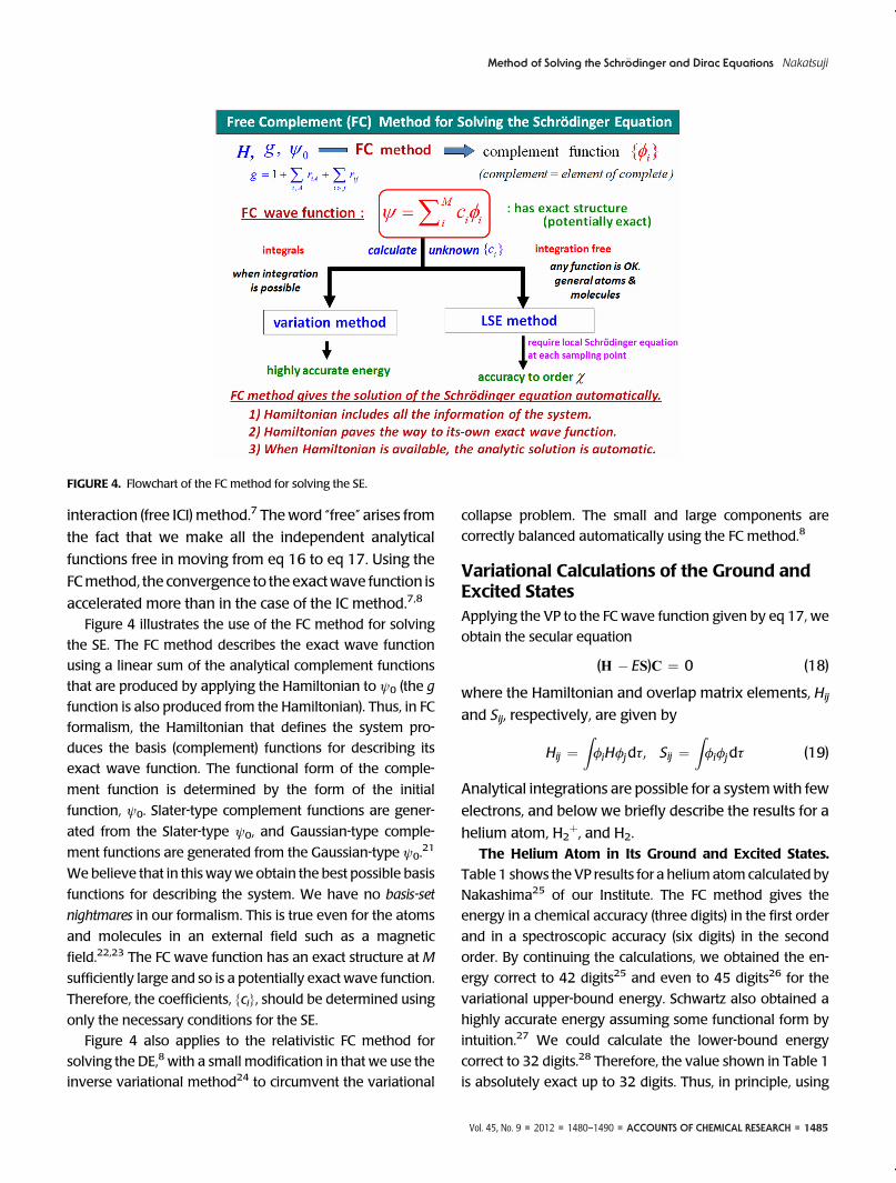
Figure 4 illustrates the use of the FC method for solving
the SE. The FC method describes the exact wave function
using a linear sum of the analytical complement functions
that are produced by applying the Hamiltonian to ψ0 (the g
function is also produced from the Hamiltonian). Thus, in FC
formalism, the Hamiltonian that defines the system pro-
duces the basis (complement) functions for describing its
exact wave function. The functional form of the comple-
ment function is determined by the form of the initial
function, ψ0. Slater-type complement functions are gener-
ated from the Slater-type ψ0, and Gaussian-type comple-
ment functions are generated from the Gaussian-type ψ0.21
We believe that in this waywe obtain the best possible basis
functions for describing the system. We have no basis-set
nightmares in our formalism. This is true even for the atoms
and molecules in an external field such as a magnetic
field.22,23 The FC wave function has an exact structure at M
sufficiently large and so is a potentially exact wave function.
Therefore, the coefficients, {ci}, should be determined using
only the necessary conditions for the SE.
Figure 4 also applies to the relativistic FC method for
solving the DE,8 with a small modification in that we use the
inverse variational method24 to circumvent the variational
collapse problem. The small and large components are
correctly balanced automatically using the FC method.8
Variational Calculations of the Ground andExcited StatesApplying the VP to the FC wave function given by eq 17, we
obtain the secular equation
(H � ES)C ¼ 0 (18)
where the Hamiltonian and overlap matrix elements, Hij
and Sij, respectively, are given by
Hij ¼ZφiHφjdτ, Sij ¼
Zφiφjdτ (19)
Analytical integrations are possible for a systemwith few
electrons, and below we briefly describe the results for a
helium atom, H2þ, and H2.
The Helium Atom in Its Ground and Excited States.
Table 1 shows the VP results for a heliumatom calculated by
Nakashima25 of our Institute. The FC method gives the
energy in a chemical accuracy (three digits) in the first order
and in a spectroscopic accuracy (six digits) in the second
order. By continuing the calculations, we obtained the en-
ergy correct to 42 digits25 and even to 45 digits26 for the
variational upper-bound energy. Schwartz also obtained a
highly accurate energy assuming some functional form by
intuition.27 We could calculate the lower-bound energy
correct to 32 digits.28 Therefore, the value shown in Table 1
is absolutely exact up to 32 digits. Thus, in principle, using
FIGURE 4. Flowchart of the FC method for solving the SE.
1486 ’ ACCOUNTS OF CHEMICAL RESEARCH ’ 1480–1490 ’ 2012 ’ Vol. 45, No. 9
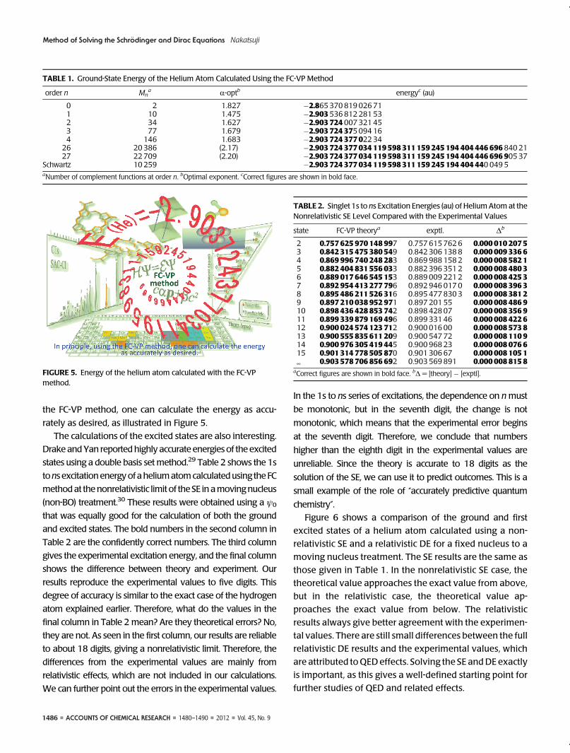
Method of Solving the Schr€odinger and Dirac Equations Nakatsuji
the FC-VP method, one can calculate the energy as accu-
rately as desired, as illustrated in Figure 5.
The calculations of the excited states are also interesting.
Drake andYan reportedhighly accurate energies of the excited
states using a double basis set method.29 Table 2 shows the 1s
tons excitationenergyof aheliumatomcalculatedusing the FC
methodat thenonrelativistic limit of the SE in amovingnucleus
(non-BO) treatment.30 These results were obtained using a ψ0
that was equally good for the calculation of both the ground
and excited states. The bold numbers in the second column in
Table 2 are the confidently correct numbers. The third column
gives the experimental excitation energy, and the final column
shows the difference between theory and experiment. Our
results reproduce the experimental values to five digits. This
degree of accuracy is similar to the exact case of the hydrogen
atom explained earlier. Therefore, what do the values in the
final column in Table 2 mean? Are they theoretical errors? No,
they are not. As seen in the first column, our results are reliable
to about 18 digits, giving a nonrelativistic limit. Therefore, the
differences from the experimental values are mainly from
relativistic effects, which are not included in our calculations.
We can further point out the errors in the experimental values.
In the 1s to ns series of excitations, the dependence on nmust
be monotonic, but in the seventh digit, the change is not
monotonic, which means that the experimental error begins
at the seventh digit. Therefore, we conclude that numbers
higher than the eighth digit in the experimental values are
unreliable. Since the theory is accurate to 18 digits as the
solution of the SE, we can use it to predict outcomes. This is a
small example of the role of “accurately predictive quantum
chemistry”.
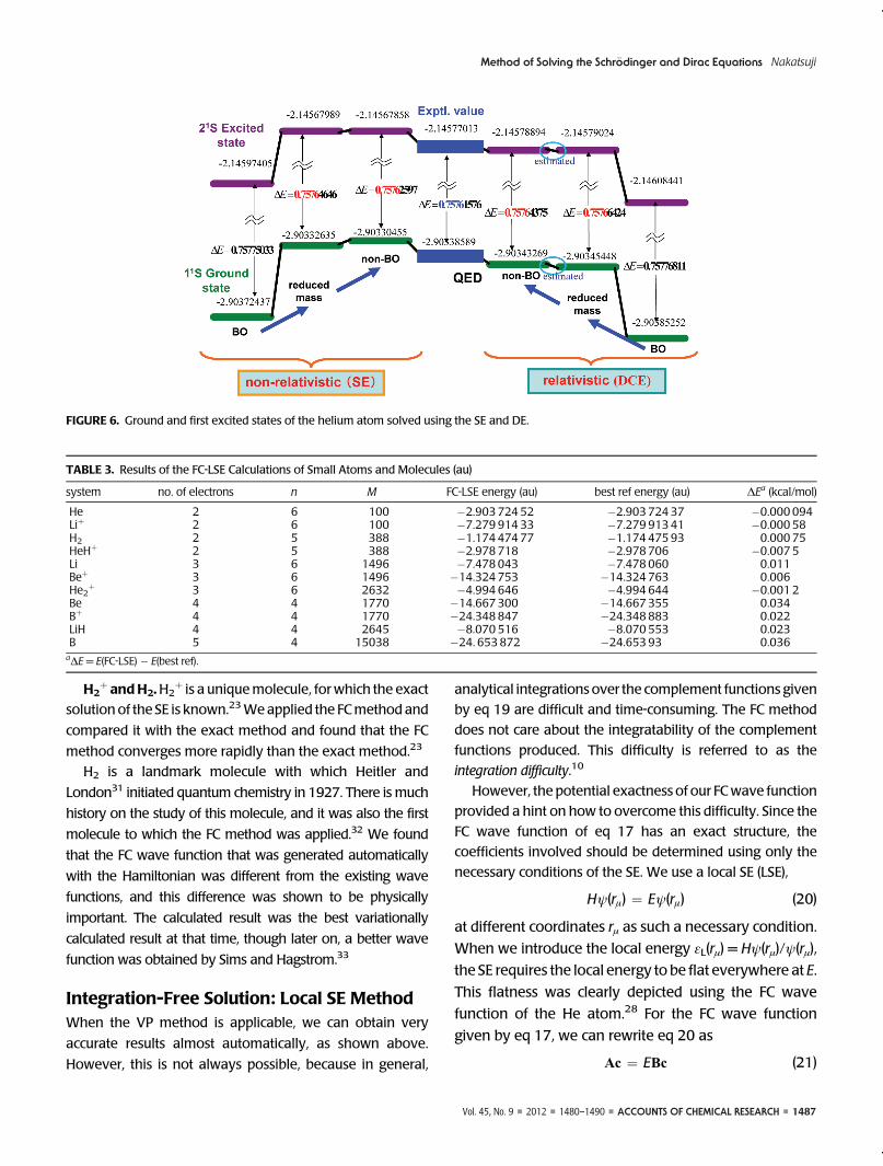
Figure 6 shows a comparison of the ground and first
excited states of a helium atom calculated using a non-
relativistic SE and a relativistic DE for a fixed nucleus to a
moving nucleus treatment. The SE results are the same as
those given in Table 1. In the nonrelativistic SE case, the
theoretical value approaches the exact value from above,
but in the relativistic case, the theoretical value ap-
proaches the exact value from below. The relativistic
results always give better agreement with the experimen-
tal values. There are still small differences between the full
relativistic DE results and the experimental values, which
are attributed toQED effects. Solving the SE andDE exactly
is important, as this gives a well-defined starting point for
further studies of QED and related effects.
TABLE 1. Ground-State Energy of the Helium Atom Calculated Using the FC-VP Method
order n Mna R-optb energyc (au)
0 2 1.827 �2.865370819026711 10 1.475 �2.903536812281532 34 1.627 �2.903724007321453 77 1.679 �2.903724375094164 146 1.683 �2.90372437702234
26 20386 (2.17) �2.9037243770341195983111592451944044466968402127 22709 (2.20) �2.90372437703411959831115924519440444669690537
Schwartz 10259 �2.9037243770341195983111592451944044400495aNumber of complement functions at order n. bOptimal exponent. cCorrect figures are shown in bold face.
FIGURE 5. Energy of the helium atom calculated with the FC-VPmethod.
TABLE 2. Singlet 1s to ns Excitation Energies (au) of HeliumAtom at theNonrelativistic SE Level Compared with the Experimental Values
state FC-VP theorya exptl. Δb
2 0.757625970148997 0.7576157626 0.00001020753 0.842315475380549 0.8423061388 0.00000933664 0.869996740248283 0.8699881582 0.00000858215 0.882404831556033 0.8823963512 0.00000848036 0.889017646545153 0.8890092212 0.00000842537 0.892954413277796 0.8929460170 0.00000839638 0.895486211526316 0.8954778303 0.00000838129 0.897210038952971 0.89720155 0.000008486910 0.898436428853742 0.89842807 0.000008356911 0.899339879169496 0.89933146 0.000008422612 0.900024574123712 0.90001600 0.000008573813 0.900555835611209 0.90054772 0.000008110914 0.900976305419445 0.90096823 0.000008076615 0.901314778505870 0.90130667 0.0000081051¥ 0.903578706856692 0.903569891 0.0000088158
aCorrect figures are shown in bold face. bΔ = [theory] � [exptl].
Vol. 45, No. 9 ’ 2012 ’ 1480–1490 ’ ACCOUNTS OF CHEMICAL RESEARCH ’ 1487
Method of Solving the Schr€odinger and Dirac Equations Nakatsuji
H2þ andH2.H2
þ is a uniquemolecule, for which the exact
solution of the SE is known.23Weapplied the FCmethod and
compared it with the exact method and found that the FC
method converges more rapidly than the exact method.23
H2 is a landmark molecule with which Heitler and
London31 initiated quantum chemistry in 1927. There is much
history on the study of this molecule, and it was also the first
molecule to which the FC method was applied.32 We found
that the FC wave function that was generated automatically
with the Hamiltonian was different from the existing wave
functions, and this difference was shown to be physically
important. The calculated result was the best variationally
calculated result at that time, though later on, a better wave
function was obtained by Sims and Hagstrom.33
Integration-Free Solution: Local SE MethodWhen the VP method is applicable, we can obtain very
accurate results almost automatically, as shown above.
However, this is not always possible, because in general,
analytical integrations over the complement functions given
by eq 19 are difficult and time-consuming. The FC method
does not care about the integratability of the complement
functions produced. This difficulty is referred to as the
integration difficulty.10
However, the potential exactness of our FCwave function
provided a hint on how to overcome this difficulty. Since the
FC wave function of eq 17 has an exact structure, the
coefficients involved should be determined using only the
necessary conditions of the SE. We use a local SE (LSE),
Hψ(rμ) ¼ Eψ(rμ) (20)
at different coordinates rμ as such a necessary condition.
When we introduce the local energy εL(rμ) = Hψ(rμ)/ψ(rμ),
the SE requires the local energy to be flat everywhere at E.
This flatness was clearly depicted using the FC wave
function of the He atom.28 For the FC wave function
given by eq 17, we can rewrite eq 20 as
Ac ¼ EBc (21)
FIGURE 6. Ground and first excited states of the helium atom solved using the SE and DE.
TABLE 3. Results of the FC-LSE Calculations of Small Atoms and Molecules (au)
system no. of electrons n M FC-LSE energy (au) best ref energy (au) ΔEa (kcal/mol)
He 2 6 100 �2.90372452 �2.90372437 �0.000094Liþ 2 6 100 �7.27991433 �7.27991341 �0.00058H2 2 5 388 �1.17447477 �1.17447593 0.00075HeHþ 2 5 388 �2.978718 �2.978706 �0.0075Li 3 6 1496 �7.478043 �7.478060 0.011Beþ 3 6 1496 �14.324753 �14.324763 0.006He2
þ 3 6 2632 �4.994646 �4.994644 �0.0012Be 4 4 1770 �14.667300 �14.667355 0.034Bþ 4 4 1770 �24.348847 �24.348883 0.022LiH 4 4 2645 �8.070516 �8.070553 0.023B 5 4 15038 �24. 653872 �24.65393 0.036aΔE = E(FC-LSE) � E(best ref).
1488 ’ ACCOUNTS OF CHEMICAL RESEARCH ’ 1480–1490 ’ 2012 ’ Vol. 45, No. 9
Method of Solving the Schr€odinger and Dirac Equations Nakatsuji
where {Aμi} = {Hφi(rμ)}, {Bμi} = {φi(rμ)}, and c is a column
vector of {ci}. The matrices A and B are highly nonsym-
metric. This method assumes the flatness of the local
energy evenly in the set of sampled points, rμ. The ground
state is the lowest solution, and the excited states are the
higher solutions. The LSEmethod is similar in spirit to the
least-squares local-energy method considered by Frost
many years ago.34
When we multiply BT from the left, we obtain
Hc ¼ ESc (22)
where Sij = ∑Σμφi(rμ)φj(rμ) and S is symmetric and positive
definite. At the integral limit, it becomes the overlap
integral between the complement functions φi and φj.
Similarly, Hij = ∑Σμφi(rμ)Hφj(rμ), which is close to the Hamil-
tonian matrix element but is nonsymmetric. On increas-
ing the number of sampling points, the results should
become closer to the variational results. TheMonte Carlo
method is one choice for sampling, but to prevent its
random behavior, we proposed the local transferable
sampling method.35 This gives continuous results that
are favorable for drawing potential curves and for calcu-
lating potential energy derivatives, such as vibrational
frequencies.As far as we use the LSE method, any complement
function is acceptable, since we do not calculate their
integrals. Therefore, it is interesting to try many different
analytical functions for ψ0 that produce complement func-
tions by applying the Hamiltonian.
FC-LSE Calculations of Atoms and MoleculesTable 3 shows the results of LSE calculations for small atoms
and molecules.10 We used a 107 Monte Carlo sampling.
Though these systems are small, the calculated energies are
highly accurate. The deviations from the known exact en-
ergies are less than 0.04 kcal/mol. In Table 4, we compare
TABLE 4. Comparison of Full-CI and FC-LSE Calculations for Be and LiHa
full CI free ICI LSE
exact energy (au) basis set M energy (au) ΔEb (kcal/mol) n M energy (au) ΔE,b (kcal/mol)
Be �14.667355 9s9p5d3f2g 3.1 � 106 �14.656767 6.6 4 1770 �14.667300 0.034LiH �8.070553 11s8p6d1f/9s8p6d1f 4.45 � 107 �8.069336 0.76 4 2645 �8.070516 0.023aReference 10. bΔE = E(FC-LSE) � E(best ref).
TABLE 5. FC-LSE Calculations of 5�12 Electron Atoms
state no. of electrons Mn FC-LSE energy (au) best ref energy (au)a ΔEa (kcal/mol)2Cþ(s2p) 5 619 �37.431433 �37.4311 �0.24Cþ(sp2) 5 657 �37.234858 (�37.2352)b (0.2)3C(s2p2) 6 2380 �37.845492 �37.8450 �0.35C(sp3) 6 2280 �37.691190 (�37.6914)b (0.1)4N 7 4332 �54.589932 �54.5892 0.43O 8 4885 �75.066821 �75.0673 0.32F 9 5508 �99.735340 �99.7338 �0.91Ne 10 1021 �128.935032 �128.9376 1.62Na 11 3816 �162.252549 �162.2546 �1.31Mg 12 2080 �200.061292 �200.053 �5aΔE = E(FC-LSE) � E(best ref) where the best reference is from ref 37. bEstimated value.
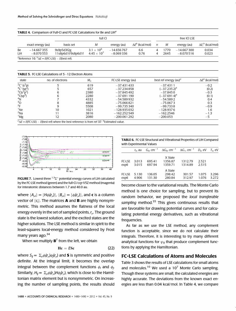
FIGURE 7. Lowest three 1,3Σþ potential energy curves of LiH calculatedby the FC-LSEmethod (green) and the full-CI/ccp-V5Zmethod (magenta)for interatomic distances between 1.7 and 40.0 au.
TABLE 6. FC-LSE Structural and Vibrational Properties of LiH Comparedwith Experimental Values
re, au G0, cm�1 ΔG0, cm
�1 ΔG1, cm�1 De, eV Te, eV
X StateFC-LSE 3.013 695.41 1356.87 1312.79 2.521exptl 3.015 697.94 1359.71 1314.89 2.515
A StateFC-LSE 5.130 136.05 298.42 301.57 1.075 3.296exptl 4.906 131.30 280.84 312.97 1.076 3.272

Vol. 45, No. 9 ’ 2012 ’ 1480–1490 ’ ACCOUNTS OF CHEMICAL RESEARCH ’ 1489
Method of Solving the Schr€odinger and Dirac Equations Nakatsuji
the FC-LSE results for Be and LiH with the full-CI results.10
Though these full-CI results used a highly accurate basis set,
the error still amounted to a fewkcal/mol, but in ourmethod,
the error was about 0.03 kcal/mol. Table 5 shows the results
for atoms with 5�12 electrons. Because carbon is especially
important, we calculated different electronic states for it. Up
to fluorine, we could obtain chemical accuracy, where the
error was less than a kcal/mol. For Ne to Mg, the errors were
larger, though it was not difficult to obtain higher accuracies.
Thus, without carrying out any integration, we could calcu-
late highly accurate energies and wave functions in an
analytical expansion form.
Potential Energy CurvesPotential energy curves and surfaces are of fundamental
importance in chemical studies. Here, we show an example
of the potential curves of the LiH molecule36 in Figure 7.
The lowest two singlet and triplet Σþ potential curves were
calculated using the FC-LSEmethod (green curves), and these
can be compared with those obtained from full-CI calcula-
tions using the cc-pV5Z basis set (magenta). The FC-LSE
curves and the full-CI curves are parallel in all the regions,
although the FC-LSE curves are always lower in energy than
the full-CI curves. The potential properties are summarized
in Table 6 and compared with the experimental values. The
equilibrium distance, re, zero-point vibrational energy, G0,
vibrational level spacing, ΔG0ΔG1, the dissociation energy,
De, and the adiabatic excitation energy between two mini-
ma, Te, show good accordance between theory and experi-
ment. The accordance is lower in the excited state, but the
very shallow nature of the potential curve leads to a fluctua-
tion in the fitted values. These results show the utility of the
FC-LSEmethod for study of chemical reactions in ground and
excited states.
Petaflops Superparallel ComputingIn recent developments in computer technology, superpar-
allel computers with petaflops to exaflops speeds are being
produced. Formost conventional quantum chemistry codes,
the adaptation to superparallel computation is not an easy
task. However, for the FC-LSE method, the most time-
consuming step is the sampling step (calculation of the
values of Hφi(rμ) and φi(rμ) in eq 21 for each sampling point
rμ). Because we usually take 105�107 sampling points in our
calculations, and each sampling point has exactly the same
computational task, superparallel computers are suitable for
FC-LSE calculations. In test calculations on N2 molecules, we
used 1152 cores in parallel and obtained an acceleration of
1150 times (99.8% parallel efficiency). We are looking
forward to the open usage of the petaflops computers at
Kobe.
Present and FutureAfter the discovery of the general theory of solving the SE,
we have investigated and developed different methods and
algorithms inorder to apply this general theory to atomsand
molecules of different sizes and in different situations. The
LSE method is one example that forced us to develop a
sampling-type methodology. The methods described here
are general, and are therefore, in principle, applicable to any
system.However, the algorithmswehave reviewedhere are
the straightforward ones derived from the original theories.
They are still time-consuming to apply to molecules familiar
in everyday chemistry, and it is therefore important to invent
more efficient methods. We are now developing several
ideas in parallel. Further, with the active research of many
scientists who are interested in this subject, we hope this
field is much cultivated and will offer innovative methodol-
ogies that make confident quantitative predictions possible
in the field of chemical science.
I acknowledge Dr. Hiroyuki Nakashima of QCRI for activecollaborations.
BIOGRAPHICAL INFORMATION
Hiroshi Nakatsuji has been the Director of the Quantum Chem-istry Research Institute since 2006 and a Professor Emeritus ofKyoto University since 2007. He is the author of the force conceptfor molecular geometries and chemical reactions, the densityequation for the direct determination of density matrix, the SACand SAC-CI theories for ground, excited, ionized, and electron-attached states of molecules, the dipped adcluster model forchemisorption and catalytic reactions on a metal surface, andstudies on the mechanisms and relativistic effects in nuclearmagnetic resonance.
FOOTNOTES
*E-mail: [email protected] authors declare no competing financial interest.
REFERENCES1 Dirac, P. A. M. Quantum mechanics of many-electron systems. Proc. R. Soc. London, Ser.
A 1929, 123, 714–733.2 Hawking, S.; Mlodinow, L. The Grand Design; Bantam Books: London, 2010.3 Piecuch, P.; Kucharski, S. A.; Kowalski, K. Can ordinary single-reference coupled-cluster
methods describe the potential curve of N2? The renormalized CCSDT(Q) study. Chem.Phys. Lett. 2001, 344, 176–184.
4 Nakatsuji, H. Structure of the exact wave function. J. Chem. Phys. 2000, 113, 2949–2956.

1490 ’ ACCOUNTS OF CHEMICAL RESEARCH ’ 1480–1490 ’ 2012 ’ Vol. 45, No. 9
Method of Solving the Schr€odinger and Dirac Equations Nakatsuji
5 Nakatsuji, H.; Davidson, E. R. Structure of the exact wave function. II. Iterative configurationinteraction method. J. Chem. Phys. 2001, 115, 2000–2006.
6 Nakatsuji, H. Inverse Schr€odinger equation and the exact wave function. Phys. Rev. A 2002,65, No. 052122.
7 Nakatsuji, H. Scaled Schr€odinger equation and the exact wave function. Phys. Rev. Lett.2004, 93, No. 030403.
8 Nakatsuji, H. General method of solving the Schr€odinger equation of atoms and molecules.Phys. Rev. A 2005, 72, No. 062110.
9 Nakatsuji, H.; Nakashima, H. Analytically solving relativistic Dirac-Coulomb equation foratoms and molecules. Phys. Rev. Lett. 2005, 95, No. 050407.
10 Nakatsuji, H.; Nakashima, H.; Kurokawa, Y.; Ishikawa, A. Solving the Schr€odinger equationof atoms and molecules without analytical integration based on the free iterative-complement- interaction wave function. Phys. Rev. Lett. 2007, 99, No. 240402.
11 Sakurai, J. J. Advanced Quantum Mechanics; Addison-Wesley: CA, 1967.12 Moore, C. E. Atomic Energy Levels; National Bureau of Standards: Gaithersburg, MD, 1971;
Vol. I.13 Nakatsuji, H. Structure of the exact wave function. III. Exponential ansatz. J. Chem. Phys.
2001, 115, 2465–2475.14 Nakatsuji, H. Structure of the exact wave function. IV. Excited states from exponential ansatz
and comparative calculations by the iterative configuration interaction and extended coupledcluster theories. J. Chem. Phys. 2002, 116, 1811–1824.
15 Nakatsuji, H.; Ehara, M. Structure of the exact wave function. V. Iterative configurationinteraction method for molecular systems within finite basis. J. Chem. Phys. 2002, 117,9–12.
16 Nakatsuji, H. Equation for the direct determination of the density matrix. Phys. Rev. A 1976,14, 41–50.
17 Nakatsuji, H. Deepening and extending the quantum principles in chemistry. Bull. Chem.Soc. Jpn. 2005, 78, 1705–1724.
18 Nakatsuji, H. Full configuration-interaction calculations with the simplest iterative comple-ment method: Merit of the inverse Hamiltonian. Phys. Rev. A. 2011, 84, No. 062507.
19 Nakatsuji, H.; Ehara, M. Iterative CI general singles and doubles (ICIGSD) method forcalculating the exact wave functions of the ground and excited states of molecules.J. Chem. Phys. 2005, 122, No. 194108.
20 Nakatsuji, H. Local g operator in the formation of the complement functions. Manuscript inpreparation.
21 Nakatsuji, H.; Nakashima, H. How does the free complement wave function becomeaccurate and exact finally for the hydrogen atom starting from the Slater and Gaussian initialfunctions and for the helium atom on the cusp conditions? Intern. J. Quantum Chem. 2009,109, 2248–2262.
22 Nakashima, H.; Nakatsuji, H. Solving the Schr€odinger and Dirac equations for a hydrogenatom in the universe's strongest magnetic fields with the free complement method.Astrophys. J. 2010, 725, 528–533.
23 Ishikawa, A.; Nakashima, H.; Nakatsuji, H. Accurate solutions of the Schr€odinger and Diracequations of H2
þ, HDþ, and HTþ: With and without Born-Oppenheimer approximation andunder magnetic field. Chem. Phys. 2012, 401, 62–72.
24 Hill, R. N.; Krauthauser, C. A solution to the problem of variational collapse for the one-particle Dirac equation. Phys. Rev. Lett. 1994, 72, 2151–2154.
25 Nakashima, H.; Nakatsuji, H. Solving the Schr€odinger equation for helium atom and itsisoelectronic ions with the free iterative complement interaction (ICI) method. J. Chem.Phys. 2007, 127, No. 224104.
26 Kurokawa, Y.; Nakashima, H.; Nakatsuji, H. Solving the Schr€odinger equation of helium andits isoelectronic ions with the exponential integral (Ei) function in the free iterativecomplement interaction method. Phys. Chem. Chem. Phys. 2008, 10, 4486–4494.
27 Schwartz, C. Experiment and theory in computations of the He atom ground state. Int. J.Mod. Phys. E 2006, 15, 877–888.
28 Nakashima, H.; Nakatsuji, H. How accurately does the free complement wave function of ahelium atom satisfy the Schr€odinger equation? Phys. Rev. Lett. 2008, 101, No. 240406.
29 Drake, G. W. F.; Van, Z.-C. Variational eigenvalues for the S states of helium. Chem. Phys.Lett. 1994, 229, 486–490.
30 Nakashima, H.; Hijikata, Y.; Nakatsuji, H. Solving the electron and electron-nuclearSchr€odinger equations for the excited states of helium atom with the free iterative-complement-interaction method. J. Chem. Phys. 2008, 128, No. 154108.
31 Heitler, W.; London, F. Wechselwirkung neutraler atome und hom€oopolare bindung nachder quantenmechanik. Z. Phys. A 1927, 44, 455–472.
32 Kurokawa, Y.; Nakashima, H.; Nakatsuji, H. Free ICI (Iterative Complement Interaction)calculations of the hydrogen molecule. Phys. Rev. A 2005, 72, No. 062502.
33 Sims, J. S.; Hagstrom, S. A. High precision variational calculations for the Born-Oppenheimer energies of the ground state of the hydrogenmolecule. J. Chem. Phys. 2006,124, No. 094101.
34 Frost, A. A.; Kellogg, R. E.; Gimarc, B. M.; Scargle, J. D. Least-square local-energy method formolecular calculations using Gauss quadrature points. J. Chem. Phys. 1961, 35, 827–831.
35 Nakatsuji, H. Local sampling method that is transferrable and gives continuity to thecalculated properties. Manuscript in preparation.
36 Bande, A.; Nakashima, H.; Nakatsuji, H. LiH potential energy curves for ground and excitedstates with the free complement local Schrodinger equation method. Chem. Phys. Lett.2010, 496, 347–350.
37 Buendia, E.; Galvez, F. J.; Maldonado, P.; Sarsa, A. Quantum Monte Carlo ground stateenergies for the atoms Li through Ar . J. Chem. Phys. 2009, 131, No. 044115.