HAL Id: hal-00991299https://hal.archives-ouvertes.fr/hal-00991299

Submitted on 15 May 2014

HAL is a multi-disciplinary open accessarchive for the deposit and dissemination of sci-entific research documents, whether they are pub-lished or not. The documents may come fromteaching and research institutions in France orabroad, or from public or private research centers.

L’archive ouverte pluridisciplinaire HAL, estdestinée au dépôt et à la diffusion de documentsscientifiques de niveau recherche, publiés ou non,émanant des établissements d’enseignement et derecherche français ou étrangers, des laboratoirespublics ou privés.

A new concept for the contact at the interface ofsteel-concrete composite beams

Samy Guezouli, Anas Alhasawi

To cite this version:Samy Guezouli, Anas Alhasawi. A new concept for the contact at the interface of steel-concretecomposite beams. Finite Elements in Analysis and Design, Elsevier, 2014, 87 (87(2014)), pp.32-42.�10.1016/j.finel.2014.01.007�. �hal-00991299�

A new concept for the contact at the interface of steel-concrete composite beams

Samy GUEZOULI and Anas ALHASAWI

National Institute of applied Sciences (INSA) of Rennes – France

Department of Civil Engineering and Planning – Structural Engineering Research Group

Abstract

This paper deals with the problem of contact at the interface of steel-concrete composite beams. The F.E. model “Pontmixte”, able to study continuous composite beams at real scale, was based on a finite element of composite beam which considers only 4 degrees of freedom per node: both longitudinal displacements of the slab and the steel beam and common vertical displacement and rotation of the whole composite cross-section. This assumption did not allow any uplift at the interface between both materials. A “new” finite element is proposed in this work with 6 degrees of freedom per node in the aim to include a contact algorithm in the model. The originality of the method is to use the Augmented Lagrangian Method to solve the contact problem at the steel-concrete interface including a new concept so-called:”Flying Node Concept”. This concept solves the problem of “continuous” contact at the interface that could sometimes occur along the beam especially in the case of distributed loads. The influence on the loading capacity of the beam and also the influence on some design variables are highlighted.

Key words: Flying Node Concept, Augmented Lagrangian Method, Contact, F.E.M., Composite beams.

1. INTRODUCTION

In the past few years, several finite element models have been proposed for the analysis of composite steel-concrete beams; most of them are based on one-dimensional beam elements with embedded interlayer slip. “Pontmixte” [1] is one of the most innovative programs able to study composite continuous beams at real scale making two numerical integrations - the first on the height of the cross-section and the second along the longitudinal axis of the beam -. Nevertheless, the first version of this model assumed that there is no uplift between the concrete slab and the steel beam. The whole composite cross-section had same vertical displacement and same rotation. This assumption prevents the prediction of possible uplift which could occur in particular loading cases for continuous beams and especially on both sides of the intermediate supports.

Huang et al. [2, 3], proposed a non-linear layered finite element procedure for predicting the structural response of reinforced concrete slabs subjected to fire. The proposed procedure based on Mindlin/Reissner (thick plate) theory includes both geometric and material non-linearities. In this study a total Lagrangian approach was adopted in which displacements are referred to the original configuration and small strains were assumed. In the case of beams subjected to fire, contact problem needs a special attention.

Amilton et al. [4], presented a family of zero-thickness interface elements developed for the simulation of composite beams with horizontal deformable connection, or interlayer slip. The proposed elements include formulations to be employed with Euler-Bernoulli as well as with Timoshenko beam theories, combined to displacement-based beam elements sharing the same degrees of freedom. The elements that can be employed for the simulation of steel-concrete composite beams, was computed more recently by Batista et al. [5] combining with the plate formulation of Huang. The proposed model used to analyse composite floor that includes interface elements appeared able to give the relative longitudinal and transversal displacements between the slab and the steel beam as-well-as the relative vertical displacements in the transverse plane.

Recently, Qureshi et al. [6], studied the effect of shear connector spacing and layout on the shear connector capacity in composite beams. A proposed 3D model (Plan dimensions: 1500 mm ×1500 mm), is loaded as a horizontal push test. This model developed with ABAQUS, includes profiled sheeting and the interfaces concerned by the contact algorithm are: (top profile sheeting – bottom of the concrete slab) and (shaft of the headed studs – surrounding concrete). Running time and convergence difficulty lead to consider 3D models inappropriate to study a continuous bridge beam at real scale.

Due to the non-linear nature of contact mechanics, such problems in the past were often approximated by special assumptions within the design process. Due to the rapid improvement of modern computer technology, one can today apply the tools of computational mechanics to simulate applications which include contact mechanisms numerically [7].

The model proposed herein takes into account the slip and lengthening-shortening nonlinear behaviours of the connection. Whatever the zone where the contact occurs after uplift, the relative vertical displacements along the longitudinal axis of the beam is obtained without interpenetration between materials.

Different methods exist to solve the contact problem [8]. For example, in penalty method, increasing the penalty factor to infinity would lead to the exact solution, but in computational application it is not possible to use very high penalty factors because of ill-conditioning of the system. The Lagrange multiplier method fulfill the contact constraints exactly by introducing additional variables; for this reason the Lagrange multiplier generate an increment in the system-matrix size. A combination of the penalty method and the Lagrangian multiplier method leads to the so-called Augmented Lagrangian Method (ALM). With this method, the penalty factor does not need to reach a high value to get the convergence of the iterative process. This method will be used in the proposed model to solve the contact problem at the interface between the concrete slab and the steel beam subjected to the inequality constraint corresponding to the non-penetrability between both materials.

For special loading cases, it could happen that the contact at the interface is not only “node-to node” and concerns a part of the finite element length. The “Flying Node Concept (FNC)” is a new method proposed in this work to make the appropriate adjustments to the final solution of the problem.

Practically, the connection design leads to a number of studs which are distributed uniformly along the continuous beam or by portions of it (Eurocode recommendations for studs’ design). This uniform distribution is generally validated by models that use a node-based connection. In order to take into account the actual continuous contact by using a node-based connection, the FNC algorithm is proposed. The main objective is to propose a longitudinal stud distribution that could be as realistic as possible by taking into account the continuous contact.

The first mesh of the beam (same as studs’ location) begins uniform and at the end of calculation, a new stud location is proposed. If the studs’ distribution does not change significantly from the beginning until the end of calculation; this means that the FNC algorithm was not activated significantly and so, no continuous contact zones have been occurred.

2. THE “NODE-TO-NODE” CONTACT

2.1 Uplift tests

Before solving the contact problem at some composite cross-sections along the beam during the loading history, other cross-sections where the uplift could occur or the contact without penetration between both materials is satisfied should be located. With the index (s) for the slab and (g) for the steel beam, the following notation is used:

d(s): Distance between the interface and the centroïd of the slab cross-section, d(g): Distance between the interface and the centroïd of the steel beam cross-section, γj: Stud slip at the node j,

( )( s ) ( s ) ( s )j j ju v θ : Horizontal displacement, vertical displacement and rotation of the slab

cross-section at the node j, ( )( g ) ( g ) ( g )

j j ju v θ : Horizontal displacement, vertical displacement and rotation of the steel

beam cross-section at the node j.

The following tests must be activated depending on the sign of the variable ( s ) ( g )j j jv vα = − :

● Case 1: the contact without penetration is satisfied at the node j � the stud is only subjected to a slip (Fig. 1).

● Case 2: the uplift of the concrete slab with the bending of the steel beam � the contact does not exist at the node j and the bolt is subjected to both slip and lengthening (Fig. 2).

● Case 3: the uplift of the concrete slab greater (in absolute value) then the uplift of the steel beam � the contact does not exist at the node j and the stud is subjected to both slip and lengthening (Fig. 3).

Figure 1 – Contact at the node j – Slip only.

Slab

Girder

( s ) ( s ) ( s )j ju d θθθθ++++

( g ) ( g ) ( g )j ju d θθθθ++++

jγγγγ

0 L

)s(d

)g(dInterface

(i) (j)

Figure 2 – Contact at the node j – Slip and (slab uplift + steel beam lowering).

Figure 3 – Contact at the node j – Slip and (slab uplift + steel beam uplift).

2.2 “Node-to-node” contact solution

2.2.1 Equilibrium equations

Augmented Lagrangian Method is used to solve the “node-to-node” contact problem. For elastic deformation in solid mechanics, the kinematically admitted displacements that satisfy a stable equilibrium state are those whom minimize the total potential energy – this is the kinematic approach –. In our problem, the total potential energy is:

t t1V .K. .F

2∆ ∆ ∆= −

(1)

with: { } [ ] { }e e ed , K K and F f∆ = = =∑ ∑ ∑

where: { }ed is the finite element displacement vector, [ ]eK is its stiffness matrix and { }ef is

its load vector.

The minimization of Eq. (1) corresponds to:

K . F 0∆ − =

(2)

The problem of partial derivative equations is replaced by a linear system of equations and the minimal value of V in classical finite element approach of unconstrained problem is:

t1Min V .F

2∆= −

(3)

2.2.2 Application of ALM to total potential energy

( s ) ( s ) ( s )j ju d θθθθ++++

( g ) ( g ) ( g )j ju d θθθθ++++

jγγγγ

0 L

)s(d

)g(dInterface

( g )jv

( s )jv

Slab

Girder

(i) (j)

( s ) ( s ) ( s )j ju d θθθθ++++

( g ) ( g ) ( g )j ju d θθθθ++++

iγγγγ

0 L

)s(d)g(d

Interface

( g )jv

( s )jv

Slab

Girder

(i) (j)

The constrained problem to solve at each node j can be written as follows:

j

Min V

sujected to 0α ≥

(4)

The problem can be solved as a series of unconstrained minimization problems. It is pointed out that the contact depends on the behaviour of the connectors. Even if the shear failure of a connector (for example) corresponds to 6 mm slip, all along the beam its maximum slip remains around 2 mm (always in elastic range) in serviceability limit state. Similar remark could be done for the tension of a connector. The use of Minimum Potential Energy in this case is then justified.

The penalty method approach gives:

2j

pV

2After each iteration : updating p

Π α = + ∑

(5)

At iteration (I), penalty method solves this problem, then at iteration (I+1) it re-solves the problem using a largest value of the penalty factor p using the old solution as the initial guess.

The ALM combines the penalty method with the Lagrangian multipliers method. The ALM uses the following constrained objective:

2j j j

j j j

pV

2After each iteration : updating p and replacing by p

Π α λ α

λ λ α

= + −∑ ∑ −

(6)

The advantage of the ALM is that unlike the penalty method, it is not necessary that p have a very large value in order to solve the original constrained problem. Instead, because of the presence of the Lagrangian multiplier λ j, p can stay much smaller.

According to Eq. (6), the modifications that have to be done to the assembled stiffness matrix and to the corresponding loading vector, at each node j, are:

(((( ))))sju (((( ))))s

jv (((( ))))sjθθθθ (((( ))))g

ju (((( ))))gjv (((( ))))g

jθθθθ jλλλλ

(((( ))))sju (((( ))))s

jN

j* p++++ j* p−−−− −−−− 1 1 1 1 (((( ))))sjv (((( ))))s

j j jT p αααα++++

(((( ))))sjθθθθ (((( ))))s

jM

(((( ))))gju (((( ))))g

jN

j* p−−−− j* p++++ ++++ 1 1 1 1 (((( ))))gjv (((( ))))g

j j jT p αααα−−−−

(((( ))))gjθθθθ (((( ))))g

jM

−−−− 1 1 1 1 ++++ 1 1 1 1 j

1p

−−−− jλλλλ jαααα−−−−

(7)

It is easy to verify that the equilibrium is satisfied in Eq. (7). The stiffness matrix remains symmetric and there is one line and one column added for each node being in contact.

In practice, it is easier to add the supplementary equations corresponding to the nodes being in contact, at the end of the initial system as shown in Eq. (8). The system of equations to be solved has finally a “variable” dimension between (n×n) and (2n×2n) maximum depending on the number of nodes being in contact (q1, q2, q3, …). In Eq. (8), each value of the Lagrangian multiplier λqi corresponds to a node qi being in contact. A penalty factor pqi will be adjusted for each node qi; its initial value is equal to 1 and it increases during iterations (multiplying by 10 at each iteration). During the material nonlinear iterative process, the number of nodes being in contact could change.

(((( ))))gnu

�

Initi

al s

yste

m

dim

ensi

on

(((( ))))gnv

nnK (((( ))))gnθθθθ

1qλλλλ “V

ariable” system

dimension

�

2qλλλλ

3qλλλλ

⋮⋮⋮⋮

(8)

2.3 “Continuous” contact solution

During the loading history, it is possible to have some zones subjected to a contact that concerns a part of the element-length and not only its nodes. This could occur in case of distributed load more than in case of concentrated loads. In order to take into account this actual phenomenon, one proposes an approach so called “Flying Node Concept (FNC)”. This method should be included in the iterative process that solves the contact problem at the interface previously described.

The FNC adapts the longitudinal mesh of the beam during the iterative process in order to take into account the “continuous” contact to a “node-to-node” connection. If the initial mesh of the beam appears unchanged at the end-loading history, it means that all the contacts have been “node-to-node”; otherwise, the final mesh will inform about the zones that have been subjected to a “continuous” contact. It is worth to mention out that these zones could sometimes appear and sometime disappear depending on the loading history of the beam. The final solution corresponding to the end-loading and to the real final mesh depends on all intermediate calculation steps. If the FNC leads to major changes to the mesh and thus to the connection in certain zones of the continuous beam, the connection should be correctly distributed in these zones during the steel beam conception.

One considers two consecutive finite elements [(i-1) – i] and [i – j] with respective element lengths 1,IL and 2,IL at iteration I (Fig. 4.a). One supposes that the test concerns the node i of

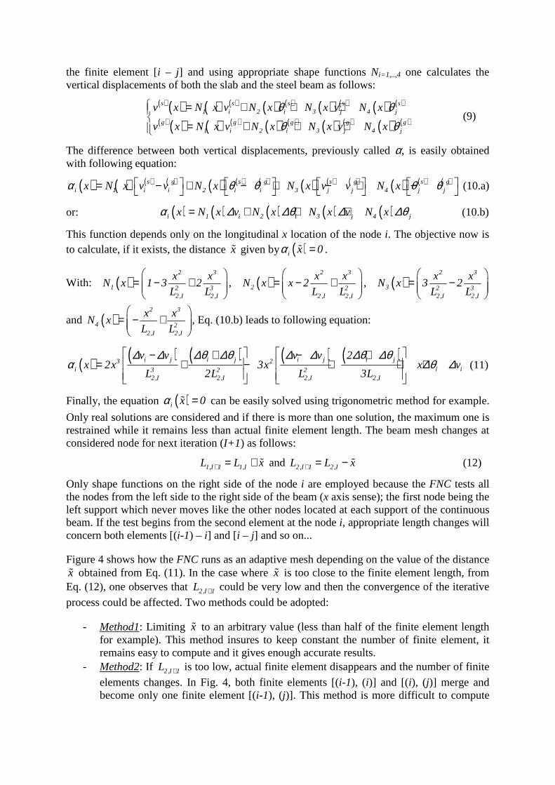
the finite element [i – j] and using appropriate shape functions Ni=1,..,4 one calculates the vertical displacements of both the slab and the steel beam as follows:

( ) ( ) ( ) ( ) ( ) ( ) ( ) ( ) ( ) ( )

( ) ( ) ( ) ( ) ( ) ( ) ( ) ( ) ( ) ( )

s s s s s1 i 2 i 3 j 4 j

g g g g g1 i 2 i 3 j 4 j

v x N x v N x N x v N x

v x N x v N x N x v N x

θ θ

θ θ

= + + +

= + + +

(9)

The difference between both vertical displacements, previously called α, is easily obtained with following equation:

( ) ( ) ( ) ( ) ( ) ( ) ( ) ( ) ( ) ( ) ( ) ( ) ( )s g s g s g s gi 1 i i 2 i i 3 j j 4 j jx N x v v N x N x v v N xα θ θ θ θ = − + − + − + − (10.a)

or: ( ) ( ) ( ) ( ) ( )i 1 i 2 i 3 j 4 jx N x v N x N x v N xα ∆ ∆θ ∆ ∆θ= + + + (10.b)

This function depends only on the longitudinal x location of the node i. The objective now is to calculate, if it exists, the distance xɶ given by ( )i x 0α =ɶ .

With: ( )2 3

1 2 32,I 2 ,I

x xN x 1 3 2

L L

= − +

, ( )2 3

2 22,I 2,I

x xN x x 2

L L

= − +

, ( )2 3

3 2 32,I 2 ,I

x xN x 3 2

L L

= −

and ( )2 3

4 22,I 2,I

x xN x

L L

= − +

, Eq. (10.b) leads to following equation:

( ) ( ) ( ) ( ) ( )i j i j i j i j3 2i i i3 2 2

2,I 2 ,I 2,I 2,I

v v v v 2x 2x 3x x v

L 2L L 3L

∆ ∆ ∆θ ∆θ ∆ ∆ ∆θ ∆θα ∆θ ∆

− + − + = + − + + +

(11)

Finally, the equation ( )i x 0α =ɶ can be easily solved using trigonometric method for example.

Only real solutions are considered and if there is more than one solution, the maximum one is restrained while it remains less than actual finite element length. The beam mesh changes at considered node for next iteration (I+1 ) as follows:

1,I 1 1,IL L x+ = + ɶ and 2,I 1 2,IL L x+ = − ɶ (12)

Only shape functions on the right side of the node i are employed because the FNC tests all the nodes from the left side to the right side of the beam (x axis sense); the first node being the left support which never moves like the other nodes located at each support of the continuous beam. If the test begins from the second element at the node i, appropriate length changes will concern both elements [(i-1) – i] and [i – j] and so on...

Figure 4 shows how the FNC runs as an adaptive mesh depending on the value of the distance xɶ obtained from Eq. (11). In the case where xɶ is too close to the finite element length, from Eq. (12), one observes that 2,I 1L + could be very low and then the convergence of the iterative

process could be affected. Two methods could be adopted:

- Method1: Limiting xɶ to an arbitrary value (less than half of the finite element length for example). This method insures to keep constant the number of finite element, it remains easy to compute and it gives enough accurate results.

- Method2: If 2,I 1L + is too low, actual finite element disappears and the number of finite

elements changes. In Fig. 4, both finite elements [(i-1), (i)] and [(i), (j)] merge and become only one finite element [(i-1), (j)]. This method is more difficult to compute

because it needs a renumbering of the mesh during the iterative process. In addition, the solution could be affected by the final mesh density that is not suitable.

Figure 4. Adaptive mesh – FNC.

In Figure 5, the FNC algorithm is shown with its links to the ALM in order to solve the contact problem. It is worth to mention out that the set of values obtained for the penalty factor p is verified by reconnecting FNC to ALM (at same contact iteration). Generally, these values are still available and the verification is directly satisfied; this is due probably to:

( )i x 0α =ɶ (Eq.10.b).

Figure 5 – Contact algorithm (ALM + FNC).

3. THE COMPOSITE BEAM F.E.

3.1 Nodal variables

The user-friendly software “Pontmixte” has been upgraded to a “new” version based on a new finite element formulation for the composite beam element. Six degrees of freedom are necessary (instead of four in the preceding version), to take into account the contact/uplift at

Slab

Girder

(i) (j)(i-1) xɶ

1,IL2,IL

Slab

Girder

(i) (j)(i-1)

1,I 1L + 2,I 1L +

Contact iteration loop « I »

ALM – test contact at each node � Contact at a node is solved � penalty factor obtained (p = pI) � Contact at a node is not solved yet � penalty factor increases (pI+1 = 10�pI)

Contact on the whole beam is solved: Each node has its own penalty factor

re-mesh the continous beamFNC

re-locate the connectors

→

Continuous contact is included Load increment: J = J+1

Loading iteration loop « J »

Ver

ifica

tion

if va

lues

of p

al

way

s av

aila

ble

the interface. The concrete slab as-well-as the steel beam has 3 degrees of freedom at each node (i) and (j) (Fig. 6). Nodal displacements vector of the composite finite element is:

{ } { }t)g(

j)g(

j)g(

j)s(

j)s(

j)s(

j)g(

i)g(

i)g(

i)s(

i)s(

i)s(

ie vuvuvuvud θθθθ= (13)

Using corresponding classical shape functions N, the displacement at each fiber of the composite cross-section is then:

{ } [ ]{ }ed( x, y ) N( x, y ) d= (14)

[ ]( ) ( )

( ) ( )

s gi i

s gj j

N 0 N 0

0 N 0 NN( x, y )

=

(15)

In Eq. (15), N includes (3×3) matrices.

The stud slip and lengthening (or shortening) are calculated considering the translation and the rotation of each material. Concerning the lengthening, the stud will be supposed fixed to the concrete:

Stud-slip: [ ] [ ])g(j

)g()g(j

)s(j

)s()s(jj dudu θ+−θ+=γ (16)

Stud-lengthening: ( s ) ( g )j j jv vα = − (17)

Figure 6 – Definition of the nodal variables.

3.2 Kinematic relationships

The kinematic variables are respectively the longitudinal strain and the curvature of each material cross-section:

( s ) ( g )( s ) ( g )x x

2 ( s ) 2 ( g )( s ) ( g )x x2 2

u u and

x x

v vand

x x

ε ε

κ κ

∂ ∂= = ∂ ∂

∂ ∂ = = ∂ ∂

(18)

Kinematic relationship and corresponding strain vector are:

{ } [ ]{ }eB dε = with { } )g(

x)g(

x)s(

x)s(

xt κεκε=ε (19)

The kinematic matrix can be written explicitly as follows:

Slab

Girder

)s(iu

)s(iv

)s(iθ

)g(iu

)g(iv

)g(iθ

)s(ju

)s(jv )s(

jθ

)g(ju

)g(jv )g(

jθ

0 L

)s(d

)g(d

Interface

[ ]

1 2 3 1 2 3

2 3 2 3

1 2 3 1 2 3

2 3 2 3

2B B y B y 0 0 0 B B y B y 0 0 0

L

20 B B 0 0 0 0 B B 0 0 0

LB

20 0 0 B B y B y 0 0 0 B B y B y

L

20 0 0 0 B B 0 0 0 0 B B

L

− − −

− − − −

=

− − −

− − − −

(20)

with: 1

1B

L= , 2 2 3

6 xB 12

L L= − , 3 2

4 xB 6

L L= −

3.3 Stiffness matrix of the composite finite element

Paying attention to the kinematic matrix, one observes that it depends on the axial x location of the concerned cross-section and on the depth y of each material-fibre at same cross-section. The composite beam cross-section is then divided into a number of horizontal fibres (m for each steel beam flange, n fibres for the steel beam web and p fibres for the slab). The algorithm undertakes firstly a Gauss-Legendre numerical integration towards the element-depth with 2 Gauss-points for each fibre (1st integration along y axis – Fig. 7). By summing different stiffnesses along y axis, the result (that corresponds to the stiffness of the composite cross-section) is affected to one of the Gauss points in order to undertake the 2nd integration along x axis (Fig. 7) that uses also 2 Gauss points.

Figure 7 – Two numerical integrations (one along each axis y and x).

In order to simplify the presentation, the first numerical integration will not appear explicitly. One begins by the element stiffness matrix of the unconnected [(i), (j)] composite beam that can be easily obtained by:

[ ] [ ][ ]L

t

e

0

K B D B dx = ∫ɶ (21)

with the behaviour matrix [ ]D in accordance with Eq.18:

m fibres

n fibres

m fibres

2 Gauss points

i j

x y

i j 2 Gauss points

y

x

2nd integration along x axis

A

A

B

B

1st integration along y axis

A-A or B-B

p fibres

[ ]

( )( )

( )( )

( s )

( s )

( g )

( g )

EA 0 0 0

0 EI 0 0D

0 0 EA 0

0 0 0 EI

=

(22)

E: Secant Young’s modulus, A: cross-section area and I: quadratic inertia of the cross-section. A secant algorithm is used to solve nonlinear equations due to nonlinear behaviour of materials.

In order to include a connector at the node (j) of the finite element [(i), (j)] for example, the principle of virtual work is applied to set the global relationship of the stud behaviour under a shear loading as-well-as under a tension.

● The internal work of an infinitesimal slip of the stud at the node (j) and corresponding nodal variables are:

{ }= = − −ss ( s ) ( g ) ssint j j j jW Q Q 1 d 1 d dδ δγ δ (23)

{ } =tss ( s ) ( s ) ( g ) ( g )

j j j j jd u uδ δ δθ δ δθ (24)

Qj is the stud shear force and d(s) and d(g) are defined in Fig. 5.

Corresponding nodal forces are: { } =tss ( s ) ( s ) ( g ) ( g )

j j j j jF N M N M (25)

● The internal work of an infinitesimal lengthening of the stud at the node (j) and corresponding nodal variables are:

{ }st stint j j j jW P P 1 1 dδ δα δ= = − (26)

{ } =tst ( s ) ( g )

j j jd v vδ δ δ (27)

Corresponding nodal forces are: { } =tst ( s ) ( g )

j j jF T T (28)

● External works related to the nodal forces given in Eq. (22) and Eq. (25) are:

{ } { }=tss ss ss

ext j jW d Fδ δ (29)

{ } { }=tst st st

ext j jW d Fδ δ (30)

● The principle of virtual works leads to:

=ss ssint extW Wδ δ (31)

=st stint extW Wδ δ (32)

The stud slip behaviour is defined as the relationship between the force at the stud head and the slip calculated between its base and the force point application. This stud slip has been defined previously in Eq. (16) and Rss is the stud slip-resistance:

=ss ss

j jQ R γ

(33)

From Eq. (31), the stud stiffness matrix ssK

related to its slip-resistance can be easily

obtained:

{ } { }{ } { }

t tss ss ss ( s ) ( g ) ( s ) ( g ) ssint j j j j

tss ss ssext j j

W Q R d 1 d 1 d 1 d 1 d d

W d F

δ δγ δ

δ δ

= = − − − − =

(34)

{ } { }tss ss ( s ) ( g ) ( s ) ( g ) ssj jF R 1 d 1 d 1 d 1 d d= − − − − (35)

The stud stiffness matrix related to its slip-resistance is finally:

( )

( )

− − − −

= − − − −

( s ) ( g )

2( s ) ( s ) ( s ) ( s ) ( g )

ss ss

( s ) ( g )

2( g ) ( s ) ( g ) ( g ) ( g )

1 d 1 d

d d d d dK R

1 d 1 d

d d d d d

(36)

Concerning the stud lengthening behaviour, same procedure then the one developed for the stud slip-resistance is carried out. The stud tension resistance is called Rst and the stud lengthening has been previously defined in Eq. (17):

st stj jP R α=

(37)

{ } { }{ } { }

t tst st st stint j j j j

tst st stext j j

W P R d 1 1 1 1 d

W d F

δ δα δ

δ δ

= = − − =

(38)

{ } { }tst st stj jF R 1 1 1 1 d= − −

(39)

The stud stiffness matrix related to its lengthening-resistance is finally:

st st 1 1K R

1 1

− = −

(40)

After replacing by the symbol (*) the terms of the stiffness matrix related to an unconnected composite beam element given in Eq. (21) concerning an unconnected composite beam, the stiffness matrix of the finite element [(i), (j)] representing a connected composite beam is:

[ ] ss ste eK K K K = + +

ɶ (41)

Respecting the nodal variables organization given in Eq. (13), this matrix can be written explicitly as follows:

[ ]

( )

( )

= + + − −

+ −

+ − −

+ +

+

+

ss ( s ) ss ss ( g ) ss

st st

2( s ) ss ( s ) ss ( s ) ( g ) ss

ss ( g ) ss

st

2( g ) ss

e

* * * 0 0 0 * * * 0 0 0

* * 0 0 0 * * * 0 0 0

* 0 0 0 * * * 0 0 0

* * * 0 0 0 * * *

* * 0 0 0 * * *

* 0 0 0 * * *

K * R * * d R R 0 d R

* R * 0 R 0

Symmetry * d R d R 0 d d R

* R * * d R

* R *

* d R

∫L

0

dx

(42)

4. NUMERICAL SIMULATION

In order to proof that the use of contact algorithm is relevent to obtain accurate results, first numerical inestigation concerns the comparision between experimental test results and the ones obtained by the “old” model with 4 degrees of freedom per node on one hand and the “new” model with 6 degrees of freedom per node on second hand.

Second numerical simulation will concerns an application for the FNC considering the same twin-beam subjected to a distributed load.

4.1. Comparison with an experimental test

The steel-concrete composite twin-beam considered (Fig. 8.a) has been subjected to an experimental test at Structural Laboratory of INSA-Rennes. The beam is loaded in accordance with the following stages:

- Stage 1: The self-weight is taken into account (4.17 kN/m for sagging zones and 4.26 kN/m for hogging ones). - Stage 2: Concentrated loads “P1” and “P2” are applied at the mid-spans of the beam until the magnitude of 550 kN for each. - Stage 3: The load “P2” remains constant and the load “P1” continue to increase from 550 kN to 850 kN.

In Figure 8.b is plotted the loading history corresponding to the stages 2 and 3, the stage 1 is not represented because it represents a distributed load and it is different on hogging and sagging zones of the continuous beam.

It is assumed that the hogging zone concerns 15% of the span length on each side of the intermediate support. For this zone, the thickness of the bottom flange is equal to 15 mm and for other cross-sections (in sagging zones) only 10 mm is required. The top flange thickness is equal to the bottom one. Related to mechanical behaviour of each material (Fig. 9), the mechanical properties are summarized in Table 1.

Figure 8.a – Geometrical characteristics of the twin-beam.

Figure 8.b – Loading stages 2 and 3.

Table 1 – Numerical values of mechanical characteristics.

Material Parameters

Concrete Ecm = 36000 MPa, fck = 40 MPa, fcm = 48 MPa, fctm = 2 MPa, εm = 0.0022,

εr(c) = 0.004

Steel beam E(a) = 190000 MPa, fy(a) = 475 MPa, fu

(a) = 620 MPa, µ1(a) = 10, µ2

(a) = 28

Rebar E(s) = 200000 MPa, fy(s) = 443 MPa, fu

(s) = 565 MPa, µ1(s) = 1, µ2

(s) = 32

Stud Qu = 80000 N, C1 = 0.7, C2 = 0.8, γmax = 6 mm

15800 P2 P1

825

1125

2250 3750 2625

x

y

φ12

φ8 180

15

70

25

110

6

120

180

10

6

1200

140

Hogging zone Sagging zone

600

180 180

Concrete: ( )( c ) 2

cm

k

f 1 k 2

σ η ηη

−=+ −

with : ( c )

m

0ηεε

= > and mcm

cm

k 1.1Ef

ε= (43)

Stud: ( ) 21

cc

uQ Q 1 e γ−= − (44)

σσσσ(c)

εεεε(c) εm

fctm

fck = αfcm

0.4fcm

εr(c)

Compression

fcm

Atan(Ecm)

σσσσ(a)

εεεε(a)

εe(a) µ1

(a)εe(a) µ2

(a)εe(a)

Atan(E(a))

fy(a)

fu(a)

Tension

a – Concrete b – Steel beam

σσσσ(s)

εεεε(s)

εe(s) µ1

(s)εe(s) µ2

(s)εe(s)

Atan(E(s))

fy(s)

fu(s)

Tension

Q

γγγγ

γmax

Qu

c – Rebar d – Stud

Figure 9 – Material mechanical behaviour.

As mentioned previously, with the assumption of 4 degrees of freedom per node, the contact at the interface could not be taken into account as-well-as possible uplifts along the beam. With this assumption, the comparison between numerical and experimental results could not be totally satisfactory. In Fig. 10 obtained from [16], the comparison of the beam deflexion between numerical and experimental results with the previous “old” model “Pontmixte” shows a significant difference especially over the elastic range. This result was predictable because the penetration as-well-as the uplift at the material interface begin to be significant when the load increases. In this figure, one observes that the deflexion under “P1” has been underestimated with this numerical model since “P1” continues to increase over 550 kN. Unfortunately the measurements under the load “P2” have not been done, but the conclusion should be similar to “P1”.

Figure 10 – Comparison of deflexions – “old” model [16].

It is clear that the effect of the interface “behaviour” becomes significant for high load level and especially under concentrated loads or at intermediate supports. For this reason, following numerical simulations, using the proposed “new” model (6 degrees of freedom per node), should help to understand how the contact algorithm could give more accurate results.

For the same twin-beam, are compared in Figures 11 some design variables obtained with the “new” finite element model. The left curves correspond to the model without activating the ALM algorithm and the right ones with activating the ALM algorithm. The left curves are plotted in the aim to identify the critical cross-sections along the beam where the ALM algorithm should be activated. In Figure 11.a and Figure 11.b are plotted respectively the comparison of vertical displacements between the slab and the steel beam and the comparison of the rotations for the last-step loading. As it was predicted, the left curves related to the cross-sections located under the concentrated loads show a penetration of the concrete slab in the steel beam. This penetration is theoretical and not realistic and it will be corrected by activating the ALM algorithm (right curves). It is pointed out that the minimum gap at the interface is fixed to 10-3 mm for these numerical simulations. This value leads to reasonable time computation for convergence of the contact iterative process. In Figure 11.c, are plotted the stud slip curves and the lengthening-shortening ones. The penetration and the uplift observed in the left curves disappear in the right curves; maximum uplift is observed at each side of the intermediate support. The slip curves become more smoothed with the ALM algorithm especially under the concentrated loads.

One observes that the use of the ALM algorithm makes changes in the magnitude of the design variables and therefore should have a special attention.

In Figure 12 are plotted similar curves as in Figure 10 but for the “new’ finite element model activating the ALM algorithm. One observes the incidence on the beam deflexion under the concentrated load “P1”; the correlation between numerical and experimental results is more satisfactory in the post-elastic range.

Without ALM algorithm With ALM algorithm

Figure 11.a – Comparison of the vertical displacement – “new” model.

Without ALM algorithm With ALM algorithm

Figure 11.b – Comparison of the cross-section rotation – “new” model.

Without ALM algorithm With ALM algorithm

Figure 11.c – Comparison of the stud slip and the stud lengthening-shortening – “new” model.

Figure 12 – Comparison of deflexions – with ALM algorithm.

4.2. Influence of the FNC

In order to show how “Pontmixte” solves the problem of the “continuous” contact, precedent twin-beam is now subjected to a distributed load p. The calculation is carried out until reaching elastic hogging bending elM − at intermediate support. Initial mesh of the twin-beam

contains 10 finite elements per beam; this mesh is called Mesh-0. The results of two calculations are compared:

- Calculation1: Contact solved with ALM

- Calculation2: Contact solved with ALM + FNC

In the aim to avoid additional differences between the results due to different numbers of finite elements, Method1 presented in 2.3 will be used in this example. Initial mesh will change several times during the loading history of the beam (Fig. 13). Only the final mesh so called Mesh-n will be highlighted because it corresponds to the last step loading. Mesh-0 and Mesh-n are presented in Figure 14. One observes that the difference between the finite element lengths mostly concerns both sides of the intermediate support and also the zones close to the end-supports. These zones correspond to the ones that are subjected to a “continuous” contact and solved by the FNC. It is pointed out that the symmetry of the problem is retained until convergence.

Figure 13 – Successive beam meshes.

Figure 14 – Comparison between initial and final mesh.

For Calculation1 and Calculation2 same stopping criterion is used: reaching elastic hogging bending at intermediate support. For Calculation1, elastic hogging bending is reached for p = 280 kN/m and for Calculation2 p = 264 kN/m. For these both loading levels, the stresses in the composite cross-sections at mid-span and at intermediate support are given in Figure 15.a and Figure 15.b.

The hogging bending is obtained when the top beam-flange reaches its yield stress (fy(a) = 475

MPa). The stress difference observed on hogging bending between both calculations is due only to the precision and it appears neglectable and same corresponding hogging bending is

S elM M 871 kN/m− −= = − . Nevertheless, in sagging zone, the stress difference is greater than

the one on hogging and should not be neglected. In Calculation2, the sagging bending is greater than in Calculation1; this explains why the elastic hogging bending is reached faster (Table 2).

Figure 15.a – Stress distribution in sagging and hogging cross-sections Calculation1 (ALM) – p = 280 kN/m.

475 MPa

147 MPa

elM −

216 MPa

SM +

− 306 MPa

−6 MPa

Sagging Hogging

−317 MPa

Figure 15.b – Stress distribution in sagging and hogging cross-sections Calculation2 (ALM + FNC) – p = 264 kN/m.

One compares now the stress distribution of both calculations for same load level (p = 264 kN/m). Figure 15.b and Figure 16 show that in Calculation1 the stresses are underestimated and the moments (Table 2) are around 3% less in sagging zone and 6% less on hogging zone. This difference is mostly due to the “continuous” contact that increases the stud slip in Calculation2 and not in Calculation1. In Figure 17 are plotted the stud-slip curves for these both calculations, maximum differences are observed in the zones that are mostly subjected to a “continuous” contact (at each side of intermediate support and near the end-supports – Fig. 14).

Figure 16 – Stress distribution in sagging and hogging cross-sections Calculation1 (ALM) – p = 264 kN/m.

Table 2 – Comparison of bending moments.

Calculation Sagging bending Hogging bending

Calculation1 (ALM) p = 280 kN/m SM 570 kN/m+ = S elM M 871 kN/m− −= = −

Calculation2 (ALM + FNC) p = 264 kN/m SM 548 kN/m+ = S elM M 871 kN/m− −= = −

Calculation1 (ALM) p = 264 kN/m SM 534 kN/m+ = S elM 821 kN/m M− −= − <

449 MPa

139 MPa

SM −

204 MPa

SM +

− 287 MPa

− 5 MPa

Sagging Hogging

475 MPa

151 MPa

elM −

231 MPa

SM +

− 304 MPa

− 7 MPa

Sagging Hogging

− 305 MPa

− 297 MPa

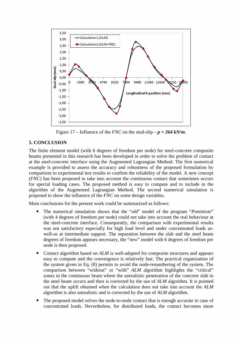
Figure 17 – Influence of the FNC on the stud-slip – p = 264 kN/m.

5. CONCLUSION

The finite element model (with 6 degrees of freedom per node) for steel-concrete composite beams presented in this research has been developed in order to solve the problem of contact at the steel-concrete interface using the Augmented Lagrangian Method. The first numerical example is provided to assess the accuracy and robustness of the proposed formulation by comparison to experimental test results to confirm the reliability of the model. A new concept (FNC) has been proposed to take into account the continuous contact that sometimes occurs for special loading cases. The proposed method is easy to compute and to include in the algorithm of the Augmented Lagrangian Method. The second numerical simulation is proposed to show the influence of the FNC on some design variables.

Main conclusions for the present work could be summarized as follows:

� The numerical simulation shows that the “old” model of the program “Pontmixte” (with 4 degrees of freedom per node) could not take into account the real behaviour at the steel-concrete interface. Consequently, the comparison with experimental results was not satisfactory especially for high load level and under concentrated loads as-well-as at intermediate support. The separation between the slab and the steel beam degrees of freedom appears necessary, the “new” model with 6 degrees of freedom per node is then proposed.

� Contact algorithm based on ALM is well-adapted for composite structures and appears easy to compute and the convergence is relatively fast. The practical organization of the system given in Eq. (8) permits to avoid the node-renumbering of the system. The comparison between “without” or “with” ALM algorithm highlights the “critical” zones in the continuous beam where the unrealistic penetration of the concrete slab in the steel beam occurs and then is corrected by the use of ALM algorithm. It is pointed out that the uplift obtained when the calculation does not take into account the ALM algorithm is also unrealistic and is corrected by the use of ALM algorithm.

� The proposed model solves the node-to-node contact that is enough accurate in case of concentrated loads. Nevertheless, for distributed loads, the contact becomes more

continuous and then the model should include the FNC. The example presented in this work shows that the loading capacity of the beam could be lower than the one predicted by a calculation without FNC (about 6% in this example). This percentage even if it remains relatively low, should be taken into account during the design of the beam because it could be not neglectable for other loading cases (for example asymmetrical distributed load on the beam). Nevertheless, more numerical simulations and experimental tests should be carried out to conclude on practical purposes.

� Solving contact problem at the steel-concrete interface has an influence on the design variables especially on the stud slip. It could be interesting to study its influence on the degree of connection in order to optimize the connection design.

REFERENCES

[1] Guezouli S. and Yabuki T., “Pontmixte” a User Friendly Program for Continuous Beams of Composite Bridges, International Colloquium on Stability and Ductility of Steel Structures (SDSS’06), Lisbon, September 6-8 2006.

[2] Huang Z., Burgess I.W. and Plank R.J., Nonlinear Analysis of Reinforced Concrete Slabs Subjected to Fire, Structural Journal, Vol. 96, Issue 1, January 1999.

[3] Huang Z., Burgess I.W. and Plank R.J., Modeling Membrane Action of Concrete Slabs in Composite Buildings in Fire, Journal of Structural Engineering, Vol. 129, Issue 8, August 2003.

[4] Amilton R. da Silva and João Batista M. de Sousa Jr., A family of interface elements for the analysis of composite beams with interlayer slip, Journal of Finite Elements in Analysis and Design, Vol. 45, Issue 5, April, 2009.

[5] João Batista M. de Sousa Jr. and Amilton R. da Silva, Analytical and numerical analysis of multilayered beams with interlayer slip, Journal of Engineering Structures, Vol. 32, n°6, 2010, pp. 1671-1680.

[6] Qureshi J., Lam D. and Ye J, Effect of shear connector spacing and layout on the shear connector capacity in composite beams, Journal of Constructional Steel Research, 67 (2011) 706-719.

[7] Kloosterman G., Contact methods in finite element Simulations, Proefschrift Enschede – Met lit. opg. – Met samenvatting in het Nederlands. ISBN 90-77172-04-1.

[8] Cavalieri F.J., Cardona A., Fachinotti V.D. and Risso J., A finite element formulation for nonlinear 3D contact problems, Mecanica Computacional, Vol. XXVI, pp. 1357-1372.

[9] Gara F., Ranzi G. and Leoni G., Displacement - based formulation for composite beams with longitudinal slip and vertical uplift, International Journal for Numerical Methods in Engineering 2006, 65(8) 1197-1220.

[10] Wriggers P., Computational Contact mechanics, Second edition, Springer-Verlag Berlin Neidelberg 2006, Printed in the Netherlands.

[11] Krofli A., Planinc I., Saje M., Turk G. and Cas B., Non-linear analysis of two layer timber beams considering interlayer slip and uplift., Journal of Engineering Structures, 2010.02.009.

[12] Krofli A., Saje M. and Planinc I., Non-linear analysis of two layer timber beams with interlayer slip and uplift, Journal of Computational Structures 2011.06.007.

[13] Robinson H. and Naraine K.S., Slip and uplift effects in composite beams, Proceedings of the Engineering Foundation Conference on Composite Construction (ASCE), 1988, pp. 487-497.

[14] Weyler R., Oliver J., Sain T. and Cante J.C., On the contact domain method: A comparison of penalty and Lagrange multiplier implementations, Computer Methods in Applied Mechanics and Engineering 205-208 (2012) 68-82.

[15] Oliver J., Hartmann S., Cante J.C., Weyler R. and Hernàndez J.A., A contact domain method for large deformation frictional contact. Problems, Part 1: Theoretical basis, Computer Methods in Applied Mechanics and Engineering 198 (2009) 2591-2606.

[16] Guezouli S., Hjiaj M. and Nguyen Q.H., Local buckling influence on the moment redistribution coefficient for composite continuous beams of bridges, The Baltic Journal of Road and Bridge Engineering (BJRBE), 2010, Vol.5, n°4, pp. 207-217.