a multiwavelength analysis of the spiral arms in the
TRANSCRIPT

Astronomy & Astrophysics manuscript no. aanda ©ESO 2021August 6, 2021
A multiwavelength analysis of the spiral arms in the protoplanetarydisk around WaOph 6
S. B. Brown-Sevilla1,?, M. Keppler1, M. Barraza-Alfaro1, J. D. Melon Fuksman1, N. Kurtovic1, P. Pinilla1, 2, M. Feldt1,W. Brandner1, C. Ginski3, 4, Th. Henning1, H. Klahr1, R. Asensio-Torres1, F. Cantalloube1, A. Garufi5, R. G. van
Holstein4, M. Langlois7, 8, F. Ménard9, E. Rickman10, 11, M. Benisty12, 9, G. Chauvin9, 12, A. Zurlo13, 14, 8, P.Weber15, 16, 17, A. Pavlov1, J. Ramos1, S. Rochat9, and R. Roelfsema18
(Affiliations can be found after the references)
Received March 11, 2021 ; accepted July 13, 2021
ABSTRACT
Context. In recent years, protoplanetary disks with spiral structures have been detected in scattered light, millimeter continuum, and CO gasemission. The mechanisms causing these structures are still under debate. A popular scenario to drive the spiral arms is the one of a planetperturbing the material in the disk. However, if the disk is massive, gravitational instability is usually the favored explanation. Multiwavelengthstudies could be helpful to distinguish between the two scenarios. So far, only a handful of disks with spiral arms have been observed in bothscattered light and millimeter continuum.Aims. We aim to perform an in-depth characterization of the protoplanetary disk morphology around WaOph 6 analyzing data obtained at differentwavelengths, as well as to investigate the origin of the spiral features in the disk.Methods. We present the first near-infrared polarimetric observations of WaOph 6 obtained with SPHERE at the VLT and compare them to archivalmillimeter continuum ALMA observations. We traced the spiral features in both data sets and estimated the respective pitch angles. We discuss thedifferent scenarios that can give rise to the spiral arms in WaOph 6. We tested the planetary perturber hypothesis by performing hydrodynamicaland radiative transfer simulations to compare them with scattered light and millimeter continuum observations.Results. We confirm that the spiral structure is present in our polarized scattered light H-band observations of WaOph 6, making it the youngestdisk with spiral arms detected at these wavelengths. From the comparison to the millimeter ALMA-DSHARP observations, we confirm that thedisk is flared. We explore the possibility of a massive planetary perturber driving the spiral arms by running hydrodynamical and radiative transfersimulations, and we find that a planet of minimum 10 MJup outside of the observed spiral structure is able to drive spiral arms that resemblethe ones in the observations. We derive detection limits from our SPHERE observations and get estimates of the planet’s contrast from differentevolutionary models.Conclusions. Up to now, no spiral arms had been observed in scattered light in disks around K and/or M stars with ages < 1 Myr. Futureobservations of WaOph 6 could allow us to test theoretical predictions for planet evolutionary models, as well as give us more insight into themechanisms driving the spiral arms.
Key words. Protoplanetary disks – Stars: individual: WaOph 6 – techniques: polarimetric
1. Introduction
The study of protoplanetary disks provides insight into ourunderstanding of the formation and early evolution of plan-ets. Modern observational techniques have enabled significantprogress to be made in this task. Recent observations in bothscattered light and millimeter continuum have shown the strik-ing frequency with which these disks present structures, such asgaps, rings, or spirals (e.g., Avenhaus et al. 2018; Long et al.2018; Andrews 2020; Cieza et al. 2020).
In particular, spiral arms have been observed in more than adozen young disks, spanning from tens to hundreds of au. Theyhave been found in scattered light (e.g., Muto et al. 2012; Wag-ner et al. 2015; Benisty et al. 2015; Stolker et al. 2016; Garufiet al. 2020; Muro-Arena et al. 2020), millimeter continuum (e.g.,Pérez et al. 2016; Huang et al. 2018b; Rosotti et al. 2020), andmore recently in CO gas emission (e.g., Tang et al. 2017; Kur-tovic et al. 2018). However, for the disks that have been imagedat different wavelengths, some of these spirals are only present
? Member of the International Max-Planck Research School for As-tronomy and Cosmic Physics at the University of Heidelberg (IMPRS-HD), Germany
in either scattered light, and not in the millimeter continuum, orvice versa. The mechanisms that drive spiral arms in these disksare probably manifold, and they are a matter of debate in manyindividual cases.
Considering that planets are born in protoplanetary disks, theobserved structures have been frequently linked with the pres-ence of planets forming within the disk (e.g., Muto et al. 2012;Pohl et al. 2015; Dong et al. 2018a; Calcino et al. 2020; Ren et al.2020). These planets perturb the disks via gravitational interac-tions, and these perturbations can cause the formation of spirals.In these cases, the planets cause spiral arms both in the interiorand exterior of their own orbit. In particular, when the planet isfairly massive, it can trigger a secondary spiral arm on the in-side of its orbit. For a planet of tens of MJup, the primary andsecondary spiral arm reach approximately a m = 21 (Dong et al.2015). From such planet-driven spirals, we can study the massand location of the potential planets. Another mechanism thatcan drive spiral arms is gravitational instability (GI, e.g., Gol-dreich & Lynden-Bell 1965). This happens when the self-gravity
1 m is the azimuthal mode number, which represents the number ofspiral arms.
Article number, page 1 of 17
arX
iv:2
107.
1356
0v2
[as
tro-
ph.E
P] 5
Aug
202
1

A&A proofs: manuscript no. aanda
perturbations in the disk dominate over the restoring forces ofgas pressure and differential rotation (Toomre 1964), which canbe translated to the disk being gas rich and relatively massivewith respect to its host star (Mdisk/M∗ & 0.1 Kratter & Lodato(2016)). Spiral arms generated by GI can allow one to better con-strain the disk mass. A third possible cause for the presence ofspiral structure is a flyby event of a close companion to the sys-tem (e.g., Cuello et al. 2019; Ménard et al. 2020) that perturbs thedisk material causing over densities that form the spiral pattern.And finally, a combination of some of the physical processes de-scribed above has also been investigated (e.g., Pohl et al. 2015).
Distinguishing between the possible physical processes driv-ing spiral structure in protoplanetary disks is not an easy task. Infact, measuring the disk gas mass alone is already challenging.Having a more comprehensive understanding of these disks canbe useful to decipher between the physical processes that are tak-ing place within them. One approach is to use multiwavelengthobservations to trace their different components. In particular,images obtained in scattered light are sensitive to micron-sizeddust grains at the disk surface, which under typical disk condi-tions are very well coupled to the gas. Images at (sub)millimeterwavelengths, on the other hand, trace larger grains within thedisk midplane, and they are less well coupled to the gas. There-fore, comparing images at these wavelengths with similar angu-lar resolution can potentially reveal the different morphologies ofdifferent disk components. Actually, it may be possible to distin-guish between planet- or GI-induced spirals by comparing scat-tered light and millimeter continuum observations, since dusttrapping in spiral arms is likely to be more efficient in gravita-tionally unstable disks (Juhász et al. 2015; Dipierro et al. 2015).Previous studies have utilized observations in both near-infrared(NIR) and millimeter continuum to analyze the disks’ morphol-ogy, as well as the gas and dust distributions within them (e.g.,van Boekel et al. 2017; Rosotti et al. 2020), however, so far thereare only a handful of such works.
In this paper, we present NIR polarimetric observations ofWaOph 6 obtained using the VLT/SPHERE instrument (Beuzitet al. 2019). These observations have a spatial resolution of∼51 mas (∼ 6 au), similar to that of the recent ALMA-DSHARPmillimeter wavelength observations (Andrews et al. 2018, seeFig. 1). We report a NIR scattered light counterpart of the inner-most spiral arms reported in Huang et al. (2018b). Additionally,we explore one of the scenarios that can give rise to the spiralpattern observed in the disk.
The paper is structured as follows: in Section 2 we introduceWaOph 6 and the previous studies on its disk. In Section 3 wedescribe our scattered light observations and data reduction pro-cedure. Our results are presented in Section 4. We describe themodeling setup and the comparison between the simulations andthe observations on Section 5. In Section 6 we discuss our re-sults, and finally in Section 7 we summarize our findings and listour conclusions.
2. Stellar and disk properties
WaOph6 is a K6 star (Eisner et al. 2005), and member of theOphiuchus moving group at a distance of 122.5 +0.3
−0.2 pc (GaiaCollaboration et al. 2020) located near the L162 dark cloud.It was first identified as a suspected T Tauri star by Henize(1976), and then confirmed by Walter (1986). Here we constrainthe stellar mass and age based on the updated photometry andGaia parallax. We retrieved the full spectral energy distribution
(SED) from Vizier2 and employed a Phoenix model of the stellarphotosphere (Hauschildt et al. 1999) with effective temperatureTeff = 4200 K (Eisner et al. 2005), surface gravity log(g)=-4.0,and an optical extinction AV = 2.8±0.3 mag calculated from theV, R, and I photometric fluxes. We integrated the stellar modelscaled to the average V magnitude and Gaia distance of 122.5pc obtaining a stellar luminosity of L∗ = 1.91+0.70
−0.51 L. Then, weplaced the source on the HR diagram and constrain a stellar massM∗ = 0.7±0.1 M and an age t = 0.6±0.3 Myr through differentsets of PMS tracks (Parsec, MIST, Baraffe; Bressan et al. 2012;Choi et al. 2016; Baraffe et al. 2015) with error bars propagatedfrom L∗ and Teff (± 100 K).
The disk around WaOph 6 has been a common target formillimeter continuum surveys looking to constrain and char-acterize the structure in protoplanetary disks (e.g., Andrews &Williams 2007; Andrews et al. 2009; Ricci et al. 2010; An-drews et al. 2018). Submillimeter Array (SMA) observationswere used along with a parametric model to constrain densitystructure parameters (Andrews et al. 2009). The disk model thatbest fitted the thermal continuum data and spectral energy dis-tribution (SED) was that of a flat cold disk with a total diskmass (gas + dust-to-gas ratio of 1:100) of 0.077 M. With obser-vations from the Australia Telescope Compact Array (ATCA),Ricci et al. (2010) analyzed and modeled the SED of WaOph 6,adopting a distance of ∼130 pc and an outer radius (Rout) inter-val of 175 − 375 au, and they find dust mass estimates (Mdust)between 8 × 10⁻⁵ M and 9.8 × 10⁻⁵ M, depending on the as-sumed dust size distribution power-law index (q = 2.5 or q = 3).More recently, WaOph 6 was observed by ALMA within theDSHARP program (Disk Substructures at High Angular Resolu-tion Project, Andrews et al. 2018). These millimeter continuumobservations showed that the disk has a set of symmetric spiralarms that extend to ∼70 au, a gap at 79 au and a bright ring at88 au (Huang et al. 2018b). The disk has an inclination (i) of47.3 and a position angle (PA) of 174.2 obtained from ellipsefitting on the dust continuum emission (see Huang et al. 2018a,for more details), and gas observations have shown that it suf-fers from mild molecular cloud contamination (Reboussin et al.2015). We summarize the stellar and disk physical parametersin Table 1, where we include the different values for the diskmass found in the literature, as well as our own Mdust estimateobtained following the procedure described in Appendix A.
Up to now, only seven disks have been known to have spi-ral arms in millimeter continuum wavelengths: WaOph 6, Elias27, IM Lup, HT Lup A, AS 205 N, MWC 758, and HD100453(Huang et al. 2018b; Kurtovic et al. 2018; Dong et al. 2018a;Rosotti et al. 2020), and only the first three are single systems.Out of these three, only IM Lup has published polarized scat-tered light observations (Avenhaus et al. 2018), however, withno spiral arms visible at these wavelengths.
3. Observations and data reduction
WaOph 6 was observed with the VLT/SPHERE high-contrast in-strument (Beuzit et al. 2019) within the DISK/SHINE (SpHereINfrared survey for Exoplanets, Chauvin et al. 2017) Guaran-teed Time Observations (GTO) program on the night of June21, 2018 (see Table 2). The observations were carried out withthe IRDIS Dual-beam Polarimetric Imaging (DPI) mode (Lan-glois et al. 2014; de Boer et al. 2020; van Holstein et al. 2020)in H-band (λc=1.625 µm; ∆λ=0.291 µm; where λc denotes the
2 http://vizier.unistra.fr/vizier/sed/
Article number, page 2 of 17

S. B. Brown-Sevilla et al.: A multiwavelength analysis of the spiral arms in the protoplanetary disk around WaOph 6
Fig. 1: ALMA 1.25 mm continuum image of WaOph 6 from theALMA-DSHARP survey (Huang et al. 2018b). The beam size isshown in the lower left corner.
Table 1: Stellar and disk parameters of WaOph 6 from the mostrecent literature.
Stellar parameters Value Ref.Spectral type K6 a
Age 0.7 Myr aDistance d 122.5 ± 5 pc b
Mass 0.9 M aRadius 2.8 R a
Temperature 4205 K aVisual magnitude (V band) 13.3 ± 0.01 mag c
Disk propertiesInclination i 47.3 d
Position angle (PA) 174.2 dGas mass1 7.7x10⁻² M eDust mass2 8x10⁻⁵ M aDust mass 1.4x10⁻⁴ M f
1 Assuming a gas-to-dust ratio of 100:1 and based on SMASED modeling.
2 Obtained with a power-law index for the grain size distri-bution q = 2.5.Notes. a) Ricci et al. (2010), b) Gaia Collaboration et al.(2020), c) Zacharias et al. (2012), d) Huang et al. (2018a),e) Andrews et al. (2009), f) This work
central wavelength and ∆λ denotes the full width at half max-imum (FWHM) of the filter transmission curve; pixel scale12.25 mas/px, Maire et al. 2016) in field stabilized mode using anapodized Lyot coronagraph, having a focal plane mask of 93 masradius (Carbillet et al. 2011). A total of four polarimetric cycleswere recorded, with 96 s of integration time per exposure, result-ing in a total integration time of about 25 minutes. Each polari-metric cycle consisted of adjusting the half-wave plate (HWP) atfour different switch angles: 0, 45, 22.5, and 67.5. At eachHWP position the two orthogonal linear polarization states aremeasured simultaneously, resulting in eight images per cycle,corresponding to the Stokes components: (I ± Q)/2, (I ∓ Q)/2,(I ± U)/2, and (I ∓ U)/2. To obtain the Stokes components Q+,Q−, U+ and U−, one orthogonal state is subtracted from the otherat each of the HWP angles. Besides the science data, star centerframes at the beginning and end of the sequence, as well as flux
Table 2: Log of observations.
Date 21-06-2018Filter H-band (1.625 µm)UT start/end 01:58:36/02:24:30Exposure time 96 sAirmass ∼1.0Seeing ∼ 0.5"Coherence time (τ0) ∼ 4 msWind speed ∼ 3.8 m/sTotal exposure time ∼ 1500 s
calibration frames were obtained. For the star center frames, thedeformable mirror (DM) waffle mode was used (see Langloiset al. 2013, for more details on this mode). Two flux calibra-tion frames (images of the target star without the coronagraph)were obtained with an exposure time of 2 s and a neutral density(ND1) filter to prevent saturation. We measure a point spreadfunction (PSF) FWHM of ∼51 mas by fitting a Gaussian func-tion to the flux frames. The weather conditions were stable dur-ing the observations with a seeing of ∼0.5", a coherence time(τ0) of ∼4 ms, and wind speed of ∼3.8 m/s. The Strehl ratio wasabout 0.7, however, the low scattered light intensity resulted in arather low signal-to-noise ratio (S/N).
For the data reduction, we used the IRDAP pipeline3 version1.3.2. (van Holstein et al. 2020). First, the pipeline preprocessesthe data by performing the usual sky background subtraction, flatfielding, bad-pixel identification and interpolation, and star cen-tering corrections. Subsequently, polarimetric differential imag-ing (PDI) is performed by applying the double-sum and double-difference method described in de Boer et al. (2020) to obtain aset of Stokes Q and U frames. Finally, the data are corrected forinstrumental polarization and crosstalk effects by applying a de-tailed Mueller matrix model of the instrument (see van Holsteinet al. 2020, for more details on the data reduction procedure),yielding the final Q and U images. The final PDI images arecorrected for true north following the procedure established byMaire et al. (2016). IRDAP then obtains the linearly polarizedintensity (PI) image using the final Q and U images, from
PI =√
Q2 + U2. (1)
Next, the pipeline computes the azimuthal Stokes parametersfollowing (de Boer et al. 2020):
Qφ = −Q cos (2φ) − U sin (2φ),Uφ = +Q sin (2φ) − U cos (2φ),
(2)
where φ is the position angle (PA) measured east of north withrespect to the position of the star. In the definition above, a posi-tive signal in the Qφ image corresponds to a signal that is linearlypolarized in the azimuthal direction, while a negative signal de-notes radially polarized light in Qφ. Uφ contains any signal po-larized at ±45 with respect to the radial direction. This meansthat for disks with low inclinations (i.e., i < 45), almost all ofthe scattered light is expected to be included as a positive sig-nal in Qφ, while the Uφ image can be considered as an upperlimit of the noise level. In the case of WaOph 6, we expect somephysical signal in the Uφ image due to the inclination of the disk(see Table 1). The resulting Qφ and Uφ images are shown in Ap-pendix B.3 https://irdap.readthedocs.io
Article number, page 3 of 17

A&A proofs: manuscript no. aanda
4. Results
4.1. SPHERE/IRDIS-DPI observations
In Fig. 2 we show the final, processed Qφ and Uφ images. Due tothe low S/N, we sharpened the images by subtracting a versionof them which was convolved by a Gaussian kernel with the sizeof 10 pixels, which removes low frequency structures, and thenwe convolved them with a Gaussian kernel of size 0.1 × FWHMto smooth the images in order to enhance the spiral features. Weobserve the launch of the spiral arms up to ∼0.3" (40 au), as seenin the Qφ image (Fig. 2, left). As mentioned in Section 3, theUφ image (Fig. 2, right) in this case contains almost no signaland can be used as an upper limit of the noise level. For a bet-ter visualization of the spiral features, we plotted the azimuthalprofile by first deprojecting the filtered Qφ image, and taking theaverage flux within the ring between ∼27 and 36 au in azimuthalbins of 15. The distance range is chosen due to the presence ofthe coronagraph at lower radii, and the S/N decrease at higherradii. In Fig. 3, we show the smoothed azimuthal profile. Thespiral arms are seen as the two peaks between 20 − 100 and200 − 310. To estimate the spiral arm intensity contrast be-tween the spiral and inter-spiral regions, we measured the peakintensities of the spiral arms in radial bins spaced by 2 au. We es-timated the inter-spiral region intensity by taking the minimumvalue in each bin. The contrast is then the ratio between the peakintensities and the inter-spiral intensities. On average, we findthe spiral arm contrast to be 1.5.
4.2. Companion candidate
We detect a companion candidate (CC) in our data as shown inthe total intensity image in the top panel of Fig. 4, where theCC is more visible than in the polarized light frames. The CC islocated at a projected distance of ∼400 au (∼3") and has a bright-ness contrast of 10−3 with respect to WaOph 6. We used archivalHST data (from 1999-01-23) as an additional epoch to performan astrometric analysis in order to verify if the CC is bound tothe system. The resulting astrometry plot is shown in the bottompanel of Fig. 4, where the black curve traces the path a stationarybackground object would have followed relative to WaOph 6 be-tween the two epochs, and the markers show the position of theCC at both the HST and the SPHERE epochs. Since the CC islocated near the final position a background object would be lo-cated at, we conclude that the object is not bound to the system,and therefore could not be considered as an external perturbercausing the spirals. We note that the CC is not reported in theGaia EDR3, despite of its presence in the two data sets describedabove.
4.3. Comparison to ALMA Observations
WaOph 6 was observed within ALMA/DSHARP (Andrews et al.2018) in Band 6, at a frequency of 239 GHz (1.3 mm). Obser-vations at these wavelengths sample the millimeter-sized dustgrains that are typically located in the disk midplane (see e.g.,Villenave et al. 2020). On the other hand, our SPHERE observa-tions trace the light scattered from submicron sized dust grainslocated at the disk surface which are typically well-coupled tothe gas. In this section we do a first comparison of the two datasets.
Table 3: Spiral pitch angles for the protoplanetary disk aroundWaOph 6.
Source Spiral arm Log. µ [] Arch. µ []SPHERE N 19.79+0.12
−0.11 19.54
S 14.04+0.07−0.06 16.05
ALMA N1 13.49+0.30−0.19 18.97
S1 18.26+0.04−0.07 15.98
N2 10.75+0.23−0.15 17.86
S2 9.09+0.21−0.10 15.26
Note: For the SPHERE data, N corresponds to the northernspiral and S to the southern spiral. In the case of the ALMAdata, N1 corresponds to the northern inner spiral, S1 to thesouthern inner spiral, N2 to the northern outer spiral andS2 to the southern outer spiral. For the Archimedean fit, thepitch angles are estimated at 35 au.
4.3.1. Radial profiles
In Fig. 5 we plot the radial intensity profiles of theSPHERE/IRDIS-DPI H-band image (teal curve), and the ALMAimage in Fig. 1 (crimson curve). The curves have been normal-ized to the maximum intensity value on each image for visual-ization purposes. In order to obtain a smooth profile, we apply aGaussian kernel of size 0.1 × FWHM to the reduced Qφ imagein Appendix B. We obtained the profiles by taking the azimuthalaverage of the image intensity in rings of radius 3 au. For this weconsidered the latest literature values for i and PA (listed on Ta-ble 1), and we use the aperture_photometry() function fromthe photutils python package, which allows to perform aper-ture photometry within elliptical annuli. This permits to get theradial profile without first deprojecting the image.
As expected from the fact that the two images trace differentdust sizes, the profiles do not perfectly overlap. A closer lookbetween 70 au and 90 au shows that the substructures created bythe gap and the ring described in Section 2, are present in bothprofiles, with a slight shift. The initial drop in the intensity of theSPHERE/IRDIS-DPI profile is due to the use of a coronagraphin these observations. The cut in the ALMA data profile can beattributed to the emission from the large grains being limited tothe central ∼130 au of the disk.
4.3.2. Spiral arms
Next, we performed a spiral search on each data set to comparethe location of the spiral arms at both wavelengths. In the caseof the SPHERE data, the spiral features are better seen when theimage is plotted in polar coordinates, where spiral arms appearas inclined lines. To obtain the polar plot we first deprojectedthe image and then converted to polar coordinates. We then usedthe python function peak_local_max from the skimage pack-age to search for the peak emission points around the location ofthe spiral arms. To trace the spirals in the ALMA data we usedtwo different images generated using the tclean task in CASA5.4.1 (McMullin et al. 2007). We used uv-taper = [‘0.010arc-sec’, ‘0.010arcsec’, ‘10deg’], and two different robust values (-1.0 and 1.0) to generate an image with higher resolution in thecentral and in the outer regions, respectively. Then, we searchedfor peak emission points along the radial direction and took the3σ emission ones as the spiral arms. We repeated this process
Article number, page 4 of 17

S. B. Brown-Sevilla et al.: A multiwavelength analysis of the spiral arms in the protoplanetary disk around WaOph 6
Fig. 2: Left: Close up of the final Qφ SPHERE/IRDIS-DPI image after removing low frequency structures (see text for details) andapplying a Gaussian kernel of size 0.1 × FWHM to smooth the images and enhance the spiral features. Right: Close up of the finalUφ image showing the positive and negative signal. The 93 mas coronagraph is indicated by the gray circle, and the cross indicatesthe position of the star. The flux is normalized to the maximum value in the Qφ image.
Fig. 3: Azimuthal profile of the deprojected Qφ image, radiallyaveraged over a ring of 0.22-0.29" (∼27 - 36 au). The two peaksat around 50 and 210 correspond to the launch locations of thetwo spiral arms. The error is taken to be 2 σ. The dashed lineindicates the location of the disk’s semi-major-axis.
in both of the images described above. The resulting spirals areshown in Fig. 6, where we overplot the retrieved spiral arms onboth the SPHERE (left) and the ALMA image (right). To obtainthe SPHERE image we followed the same procedure describedin Section 4 with a Gaussian kernel of size 0.2 × FWHM. We didthis to match the scaling of the ALMA image for better compari-son purposes. To generate the ALMA image, we used the frank(Jennings et al. 2020) tool to remove the azimuthally componentof the emission of the disk and leave only the nonaxisymmetricfeatures, as described in the Appendix C. We note that the spi-ral pattern is much more prominent in the mm continuum thanin scattered light. Besides the low S/N of the SPHERE data andthe fact that the disk has been reported to be cold, this couldalso be explained by the anisotropic scattering properties of thedust of different sizes. For a disk that is not edge-on, the largerthe particles on the surface layer compared to the wavelength,the more they will scatter light into the disk in forward scatter-ing. Therefore, the amount of light scattered in the line of sight
direction would be smaller and would not be detected in scat-tered light images (e.g., Mulders et al. 2013). Additionally, wenotice that there appears to be a break in the spiral arms on theALMA image at ∼0.16" (∼20 au), which cannot be observed inour SPHERE data. In the following we treat this break as a sep-arate set of spirals.
In order to characterize the spirals we considered two mod-els. A logarithmic spiral given by:
r = r0 · exp(bθ), (3)
and an Archimedean spiral, defined as:
r = r0 + bθ, (4)
where θ is the polar angle, r0 is the radius for which θ=0, andb relates to the pitch angle (µ) of the spiral. The pitch angle isdefined as the angle between the tangents to a spiral arm and acircle drawn from the center of the disk, it describes how tightlythe spiral arms are wound. In the logarithmic case, the pitch an-gle is constant along all radii and it is given by µ = arctan(1/b),while for the Archimedean spiral, the pitch angle depends on theradius as µ = b/r. To test the symmetry of the spiral arms, theparameters r0 and b were fitted separately, while we assumed iand PA to be fixed and equal to the literature values shown inTable 1. Therefore, we had four and eight free parameters for theSPHERE and ALMA data, respectively. To fit the data, we usedthe MCMC code based on emcee (Foreman-Mackey et al. 2013)and described in Kurtovic et al. (2018). A flat prior probabilityis used for the free parameters. For each fit, we used 250 walkerswith two consecutive burning stages of 1000 and 500 steps, andthen 1500 steps to sample the parameter space.
The resulting pitch angles for each fit are given in Table 3,where for the SPHERE data, N corresponds to the northern spiraland S to the southern spiral; and in the case of the ALMA data,N1 corresponds to the northern inner spiral, S1 to the southerninner spiral, N2 to the northern outer spiral and S2 to the south-ern outer spiral. For the Archimedean fit, the pitch angles areestimated at 35 au. We find that there are some significant differ-ences between the values of the inner and outer ALMA spirals
Article number, page 5 of 17

A&A proofs: manuscript no. aanda
400 200 0 200 400x [au]
400
200
0
200
400
y[a
u]4 3 2 1 0 1 2 3 4
RA [arcsec]4
3
2
1
0
1
2
3
4
Dec
[arc
sec]
N
E
Fig. 4: Top: Total intensity SPHERE/IRDIS-DPI image ofWaOph 6. Encircled in red is the CC. Bottom: Astrometry plotof the CC of WaOph 6. The markers show the position of theCC, at the initial HST epoch, and further in time at the SPHEREepoch. The black curve traces the path a stationary backgroundobject would have followed relative to WaOph 6 between the twoepochs.
for the logarithmic model, which leads us to conclude that thetwo sets might not be part of the same spiral arm. There seemsto be additional structure in the region of the discontinuity, how-ever, follow-up deeper observations would be needed to drawany conclusions of the origin of this break. Furthermore, we notethat the values of the pitch angle for the corresponding spiralsdiffer from one data set to the other, and that in the case of theArchimedean model, the scattered light pitch angles are slightlyhigher that those from submillimeter. This can be expected, sincewe are tracing different regions of the disk (the flared surface vs.the midplane). Moreover, we find that the pitch angles from theArchimedean model decrease with the distance from the star, inagreement with the results of Huang et al. (2018b).
Figure 7 shows the spirals retrieved from both data sets in apolar map, along with the best-fit Archimedean model for each
20 40 60 80 100 120 140Distance [au]
10 3
10 2
10 1
100
Norm
alize
d in
tens
ity [a
rb.]
Gap
Ring
SPHERE/PDIALMA
Fig. 5: Radial intensity profiles of both the SPHERE and ALMAimages of WaOph 6. Plotted on a logarithmic scale and normal-ized to the maximum intensity of each image. The SPHERE pro-file is taken from the reduced Qφ image with an applied Gaussiankernel of size 0.1 × FWHM to smooth the curve, and it is shownup to 3σ of the intensity. The dotted line indicates the corona-graph coverage.
arm. We find a discontinuity in the spiral arms for the ALMAdata at ∼50 au. This peculiarity has already been reported byHuang et al. (2018b), who also noted that this discontinuity ap-pears to coincide with a region where there is additional brightemission between the main spiral arms, and comment that itcould be explained by either the presence of a ring crossing thisregion, or "spurs" emerging from the main spirals.
4.4. Origin of the spirals
Large perturbations in the disk launch sound waves that result ina spiral shape due to the differential rotation of the disk. Theo-retical models have shown that such large perturbations can bedriven by the presence of an embedded planetary mass perturber(e.g., Boccaletti et al. 2013), GI (e.g., Goldreich & Tremaine1979; Tomida et al. 2017), or a combination of both (e.g., Pohlet al. 2015).
Two-arm spirals in disks can be driven by a massive, giantplanetary companion (& 5MJ), that would typically be located atthe tip of the primary arm. This scenario suggests, however, thatthese planets are fainter than predicted by "hot-start" evolution-ary models (Dong et al. 2018b), since the number of detectionsis low.
On the other hand, one criteria to test the GI hypothesis is touse the so called Toomre (1964) parameter Q, given by
Q ≡Ωkcs
πGΣ, (5)
where Ωk is the angular velocity, cs is the sound speed, and Σis the surface density. These parameters vary with radius in thedisk, resulting in Q being a function of the radius. The Toomrestability criteria states that a disk will be gravitationally stable ifQ ≥ 1 and unstable if Q < 1.
In the case of WaOph 6, we estimated the Toomre parame-ter Q using equation 5 and assuming Σ ∝ 1/
√r, where r is the
distance from the star, throughout the disk (see Appendix D forthe detailed calculation) in order to see whether the disk would
Article number, page 6 of 17
S. B. Brown-Sevilla et al.: A multiwavelength analysis of the spiral arms in the protoplanetary disk around WaOph 6
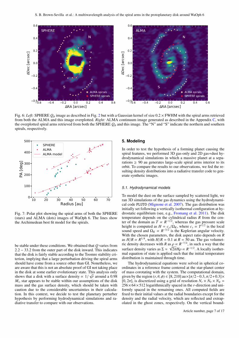
Fig. 6: Left: SPHERE Qφ image as described in Fig. 2 but with a Gaussian kernel of size 0.2 × FWHM with the spiral arms retrievedfrom both the ALMA and this image overplotted. Right: ALMA continuum image generated as described in the Appendix C, withthe overplotted spiral arms retrieved from both the SPHERE Qφ and this image. The “N” and “S” indicate the northern and southernspirals, respectively.
10 20 30 40 50 60 70Radius [au]
0
100
200
300
400
500
PA[d
eg]
SPHEREALMAALMA model
Fig. 7: Polar plot showing the spiral arms of both the SPHERE(stars) and ALMA (dots) images of WaOph 6. The lines showthe Archimedean best fit model for the spirals.
be stable under these conditions. We obtained that Q varies from2.2 − 33.2 from the outer part of the disk inward. This indicatesthat the disk is fairly stable according to the Toomre stability cri-terion, implying that a large perturbation driving the spiral armsshould have come from a source other than GI. Nonetheless, weare aware that this is not an absolute proof of GI not taking placein the disk at some earlier evolutionary state. This analysis onlyshows that a disk with a surface density ∝ 1/
√r around a 0.98
M star appears to be stable within our assumptions of the diskmass and the gas surface density, which should be taken withcaution due to the considerable uncertainties in their calcula-tion. In this context, we decide to test the planetary perturberhypothesis by performing hydrodynamical simulations and ra-diative transfer to compare with our observations.
5. Modeling
In order to test the hypothesis of a forming planet causing thespiral features, we performed 3D gas-only and 2D gas+dust hy-drodynamical simulations in which a massive planet at a sepa-rations ≥ 90 au generates large-scale spiral arms interior to itsorbit. To compare the results to our observations, we fed the re-sulting density distributions into a radiative transfer code to gen-erate synthetic images.
5.1. Hydrodynamical models
To model the dust on the surface sampled by scattered light, weran 3D simulations of the gas dynamics using the hydrodynami-cal code PLUTO (Mignone et al. 2007). The gas distribution wasinitially set following a vertically isothermal configuration at hy-drostatic equilibrium (see, e.g., Fromang et al. 2011). The disktemperature depends on the cylindrical radius R from the cen-ter of the domain as T ∝ R−1/2, whereas the gas pressure scaleheight is computed as H = cs/ΩK , where cs ∝ T 1/2 is the localsound speed and ΩK ∝ R−3/2 is the Keplerian angular velocity.With the chosen parameters, the disk aspect ratio depends on Ras H/R ∝ R1/4, with H/R = 0.1 at R = 50 au. The gas volumet-ric density decreases with R as ρ ∝ R−7/4, in such a way that thesurface density varies as Σ ≈
√2πHρ ∝ R−1/2. A locally isother-
mal equation of state is applied such that the initial temperaturedistribution is maintained through time.
The hydrodynamical equations were solved in spherical co-ordinates in a reference frame centered at the star-planet centerof mass corotating with the system. The computational domain,given by the region (r, θ, φ) ∈ [8, 210] au×[π/2−0.3, π/2+0.3]×[0, 2π], is discretized using a grid of resolution Nr × Nθ × Nφ =256×64×512 logarithmically spaced in the r-direction and uni-formly spaced in the remaining ones. All computed fields arefixed to their initial values at the radial boundaries except for thedensity and the radial velocity, which are reflected and extrap-olated in the ghost zones, respectively. On the vertical bound-
Article number, page 7 of 17

A&A proofs: manuscript no. aanda
Fig. 8: Radiative transfer images showing the spirals formed by a 10 MJup planet at 140 au. Left: Synthetic polarized scatteredlight Qφ image with an analogous Gaussian kernel to the one applied to Fig. 6, left. The dark central area shows the coronagraphcoverage. Right: Synthetic mm continuum image after subtracting the azimuthal average flux on the image plane to enhance thespirals, analogous to the procedure applied to Fig. 6, right. The red and white dots denote the location of the observed spirals foreach image, respectively.
aries, reflective conditions are applied. The gravitational poten-tial is computed as the sum of the potentials of the star and theplanet. To avoid divergences, the later is modified in the vicinityof the planet location following the prescription by Klahr & Kley(2006), employing a smoothing length equal to half the planet’sHill radius. For stability purposes, the planet mass is smoothlyincreased from 0 to its final value in a total time of 100 yr. Wealso included viscosity with constant α = 10−3. The resultingdust mass distribution was computed assuming a perfect cou-pling between the dust particles and the gas flow, with a uniformdust-to-gas mass ratio of 10−2.
To model the dust evolution in the midplane sampled mainlyby the millimeter observations, we ran two-dimensional hydro-dynamical simulations using the multi-fluid version of the codeFARGO3D4 (Benítez-Llambay & Masset 2016; Benítez-Llambayet al. 2019). It solves the Navier-Stokes equations of the gasand multiple dust species, each one modeled as a pressurelessfluid that represents a specific grain size. We traced eight differ-ent dust species in our simulations. The initial gas temperature,gas surface density structure, equation of state and gas viscosityprescription of the 2D model are equivalent to our 3D simula-tions model, described above. The initial dust surface density inour simulation has the same structure as the gas surface density,while set by an initial dust-to-gas mass ratio of 10−2 everywherein the disk. We traced the dynamical evolution of eight dust flu-ids, that are logarithmically spaced in size, and followed a dustsize distribution n(s) ∝ s−2.5 with minimum and maximum dustsizes of 10 µm and 100 µm. We set the dust intrinsic density to2.0 g cm−3. The dynamics of the dust fluids is dictated by itslocal Stokes number (dimensionless stopping time), defined asSt = πaiρint/2Σg, where ai is the grain size of the size-bin, ρintthe intrinsic grain density and Σg the gas surface density. Dustdiffusion was included in the simulation following the same pre-scriptions implemented in Weber et al. (2019), which are basedon the results of Youdin & Lithwick (2007). Dust feedback onto
4 http://fargo.in2p3.fr
the gas, dust growth, and dust fragmentation were not includedin our simulations. The two-dimensional grid is linear in azimuthand logarithmic in radius, using 512 cells in φ covering 2π, and256 cells in r covering from ∼ 8.4 au to ∼ 420 au. A planet wasslowly introduced over 8× 10⁴ yr fixed at the given radius, driv-ing spiral density waves in the disk. The planet’s potential wassmoothed by a length factor of 60% the disk scale height. Fora more detailed description of the FARGO3D multi-fluid sim-ulations see also Weber et al. (2019). Our test runs show thatonly dust fairly well coupled to the gas follows the spiral den-sity waves (as shown by e.g., Veronesi et al. 2019; Sturm et al.2020), with Stokes numbers below ∼ 10−2. Dust particles withlarger Stokes number decouple from the gas and form axisym-metric rings. Fixing the disk gas surface density given the massconstraint from the observations, and the dust intrinsic density toa standard value, limiting the maximum dust size to 100 µm inour models is required to maintain the Stokes number of the dustobserved at millimeter wavelengths below ∼ 10−2, therefore, thesimulated dust particles trace the spiral arm structure. A sum-mary of the parameters used in our simulations can be found inTable 4.
We sample the parameter space of a planet with masses be-tween 2 − 15 MJup and separations between 90 − 160 au (seeAppendix E, Fig. E.1 for some of the resulting density maps).The lower limit in the mass range is chosen based on the re-sults of Juhász et al. (2015), who concluded that observable spi-ral arms are formed for planets with M > 1MJup. Tighter con-straints on the lower limit of the planet mass can be obtainedfrom spiral arm formation theory. For a planet with a mass largerthan three thermal masses (Mth ≡ c3
s/ΩG = M?(h/r)3p), two
spiral arms will form interior to its orbit (Bae & Zhu 2018).Since we wanted to model m = 2 spirals, we chose to placethe planets outside of the spiral arm (which extends up to 90au in the millimeter continuum) based on the results of Donget al. (2015). Assuming that the planet is outside ∼ 90 au and thedisk aspect ratio of our model, we obtained that two spirals are
Article number, page 8 of 17

S. B. Brown-Sevilla et al.: A multiwavelength analysis of the spiral arms in the protoplanetary disk around WaOph 6
Table 4: Summary of simulations parameters.
Parameter 2D gas+dust 3D gasAspect Ratio at 100 au 0.12 0.12
Flaring Index 0.25 0.25Surface Density Slope 0.5 0.5
Alpha Viscosity 10−3 10−3
Stellar Mass 0.98 M 0.98 MPlanet-to-Star Mass Ratio 10−2 10−2
Planet Orbital Radius 140 au 140 au# of Cells in r 256 256# of Cells in φ 512 512# of Cells in θ - 64
Grid Inner Radius 8.4 au 8 auGrid Outer Radius 420 au 210 au
Total Evolution Time 4 × 10⁵ yr 4 × 10⁵ yrDust-to-Gas Mass Ratio 10−2 -
Maximum Dust Size 100 µm -Minimum Dust Size 10 µm -
Dust Size Slope 2.5 -Dust Intrinsic Density 2.0 g cm−3 -
formed for planet masses larger than ∼ 4.8 MJup. Another crite-ria for the planet mass comes from the separation between theprimary and secondary spiral arms (φsep). Fung & Dong (2015)obtained that this quantity scales with the planet mass, followingφsep = 102(q/0.001)0.2, where in this case q is the planet-to-star mass ratio. If we consider that the spiral arms have a sep-aration range between 135 and 180, we obtain that the planetmass should be between 4 and 17 MJup. After a few test runsin our simulations, we realized that in order to observe the disktruncate at 90 au (consistent with the disk outer edge in the mil-limeter continuum), when increasing the separation, we shouldalso increase the planet mass. Snapshots of the gas and total dustsurface densities of our 3D and 2D hydro simulations for plan-ets of 5, 10 and 15 MJup at separations of 130, 140 and 160 au,respectively, are shown in the Appendix E.
5.2. Radiative transfer
In order to compare the results generated by the procedure de-scribed in the last section with our observations, we generatedimages in both polarized NIR and millimeter continuum usingthe radiative transfer code RADMC-3D (Dullemond et al. 2012).We obtained synthetic scattered light images using the dust massdistribution computed in the described 3D PLUTO simulations.Based on Ricci et al. (2010), we assumed a dust size distri-bution n(s) ∝ s−2.5 and model scattering by submicron parti-cles with sizes ranging between 0.01 and 0.5 µm. To computethe dust mass in this range, we used the total dust mass es-timated in this work (see Table 1) assuming maximum grainsizes in the mm, to obtain Mdust,<0.5 µm = 10−9 M. Opacitiesare computed assuming a dust composition of 60% astronomi-cal silicates and 40% amorphous carbon grains, taking the opti-cal constants respectively from Draine & Lee (1984) and Li &Greenberg (1997), and combining them following the Brugge-man mixing rule. Scattering matrices were computed assumingspherical dust grains using the BHMIE code (Bohren & Huffman1983) for Mie scattering. For the scattered light computations,we approximated the grain size distribution using 5 size bins.To smooth out oscillations in the polarization degree occurringwhen considering spheres of a single size (see, e.g., Keppler et al.
2018), we used a Gaussian size distribution within each bin witha FWHM of 20% of the corresponding grain size. The star wasmodeled as a point source located at the domain center emittingthermal radiation with characteristics summarized in Table 1. Weused RADMC-3D to model anisotropic scattering with full treat-ment of polarization, using a total of 108 photon packages. Theobtained Stokes Q and U frames were then convolved by a Gaus-sian PSF with a FWHM of 51 mas to reproduce the resolution ofthe VLT/SPHERE observations (see Section 3), after which weused equation (2) to obtain the resulting Qφ images.
To compare with the ALMA data, we computed radiativetransfer predictions of the dust continuum, in this case, using theoutput of the dust and gas 2D simulation. We used the dust den-sity field from the simulation as input for RADMC-3D. We ex-panded the two-dimensional surface density vertically, assuminga Gaussian shape, where the volumetric mass density for eachdust bin follows:
ρi(r) =Σi(r)√
2πHi(r)× exp
− z2
2H2i
, (6)
where Hi indicates the pressure scale height of the dust bin. Thevertical settling of the disk follows a standard diffusion model(Dubrulle et al. 1995):
Hi =
√α
α + S tiHg, (7)
where Hg is the gas pressure scale height, S t is the dust Stokesnumber, and α = α/S cz with α the α-viscosity value of the gas.S cz is the Schmidt-number, set to 1 S cz relates the dust diffusioncoefficient with the gas viscosity Dz = ν/S cz (see also Weberet al. (2019)). We used optool5 to compute the dust asorption andscattering opacities of a mixture using standard Mie theory andBruggeman rules. We assumed that the composition of the dustgrains is a mixture of silicates (internal density of 3.2 g/cm3),amorphous carbon (internal density of 2.3 g/cm3), and vacuum.Assuming that the solids in the mixture are 60% silicates and40% carbon, a volume fraction of 25% of vacuum in the mix-ture is required so its internal density is ∼ 2 g/cm3. The dust sizedistribution is equal to the values used for the simulation, set bythe power law n(s) ∝ s−2.5, with maximum and minimum dustsizes of 100 µm and 10 µm, respectively. The total dust mass inour models is ∼ 10−4 M. We computed the dust temperature us-ing the Monte Carlo method of Bjorkman & Wood (2001), andthe continuum emission image via ray-tracing, taking into ac-count absorption and scattering, assuming Henyey–Greensteinanisotropic scattering. We computed simulated ALMA observa-tions from the radiative transfer synthetic continuum image us-ing CASA (version 5.6) simobserve and tclean tasks. Follow-ing the observations setup from the DSHARP survey (Andrewset al. 2018), we simulated an 8 h integration in configurationC43-8 combined with a 15 min integration in C43-5. Finally,we cleaned the image using briggs weighting 1.0. We obtained abeam size of 55×53 mas and PA of ∼ −55, directly comparableto the ALMA observation.
5.3. Results and comparison to observations
All tested planets drive m = 2 spiral arms whose symmetryincreases for larger planetary mass and have a low contrast inthe dust surface density (as seen in the density plots shown inFig. E.1). Given the asymmetry in the 5 MJup case, we conclude
5 https://github.com/cdominik/optool
Article number, page 9 of 17

A&A proofs: manuscript no. aanda
that in case the spirals are caused by a planet, its mass should beat least of approximately 10 MJup. In Fig. 8 we show resultingradiative transfer images for a 10 MJup planet at a separation of140 au, with spiral arms observable both in the scattered lightand millimeter continuum observations. For a better comparisonto the simulations, we apply a Gaussian kernel to the image onthe left panel, similar to the one used for the SPHERE image inFig. 6, left; and we subtract the azimuthal average flux on theimage plane to enhance the spirals on the synthetic millimetercontinuum image on the right, analogous to the procedure ap-plied to Fig. 6, right. Additionally, we overplot the location ofthe observed spiral arms. The obtained images resemble the onesdetected both in the scattered light and millimeter continuum ob-servations, except for the fact that we are only able to fit eitherthe inner or the outer spirals from the millimeter observations,but not both at the same time (see Fig. E.2, lower panel). This islikely due to missing physics in our simulations, as these modelsof spirals launched by a single planet are unable to reproduce thebreak in the spirals observed by ALMA, as well as the gap andthe ring features (at 79 and 88 au, respectively) in the observa-tions. We must also note that in order to see spiral arms inducedby a planet in millimeter continuum, the dust must be fragmen-tation limited (e.g., Birnstiel et al. 2010) leading to a small dustmaximum size, and therefore, to Stokes numbers small enoughto follow the spirals. In protoplanetary disks, the maximum grainsize is mainly set by radial drift or fragmentation of particlesafter collisions. The later depends on the disk viscosity and thethreshold considered for the fragmentation velocity of the grains.Assuming low fragmentation velocities for ice grains (e.g., <1 m/s, as suggested by recent laboratory experiments such asMusiolik & Wurm 2019; Steinpilz et al. 2019), and alpha=10−3(as taken in the simulations), the maximum grain size in the en-tire disk is dominated by fragmentation, limiting the maximumsize of 100µm (Pinilla et al. 2021). Kataoka et al. (2016) havefound that dust with similar characteristics is traced by millime-ter continuum observations of the similarly young disk HL Tau.These characteristics are not required to see spirals generatedby GI, where the dust trapping in spirals is efficient for largerdust Stokes numbers (Rice et al. 2004). We also note that noneof the parameter sets that we sample are able to reproduce thecontrast nor the apparent break in the spiral arms shown in theALMA data, which might be explained by additional physicalprocesses occurring in the disk. However, more complex simu-lations including other effects (e.g., dust growth, fragmentation,dust feedback, gas temperature evolution) are beyond the scopeof this work. Additionally, we note that a planet of 10 MJup insuch a young disk could have either formed via gravitationalcollapse when the disk was probably more massive and, there-fore, gravitationally unstable (Boss 1997), or formed as a stel-lar companion from cloud fragmentation due to the planet/starmass ratio (∼1%, Reggiani et al. 2016). We would like to men-tion that this is a first attempt to find a plausible planetary modelto explain the observed spiral pattern in the protoplanetary diskaround WaOph 6 and that further, deeper observations would beneeded to confirm or discard this scenario.
Since we employ an isothermal equation of state, the spiralsproduced in our simulations are induced solely by Lindblad res-onances and not by buoyancy modes, which may be triggeredwhen using finite cooling times. It is argued in Bae et al. (2021)that such modes cannot be observed in millimeter continuum ob-servations, but could potentially be seen in scattered light. Thepitch angles for buoyancy resonances shown in that work for upto 2 MJup planets are generally below those seen in our SPHEREobservations (see Table 3), which suggests that the observed spi-
rals are likely not triggered by such modes. Future resolved COline emission observations analyzing the disk kinematic struc-ture could help discard or verify this hypothesis (Bae et al. 2021).
6. Discussion
6.1. Observations in NIR and mm
Our SPHERE/IRDIS-DPI observations show the launch of anm = 2 spiral pattern in the disk around WaOph 6. This is asurprising finding, since so far, no spiral arms had been ob-served in scattered light in disks around K and/or M stars withages < 1 Myr. Moreover, spiral arms have not been observedat these wavelengths in single T Tauri stars of any age (Garufiet al. 2018). Disks with spiral arms detected in scattered light arethought to be older (with the caveat that stellar ages are highlyuncertain), and with stellar hosts of spectral types from G to A(e.g., MWC 758, Dong et al. (2018a), HD 142527, Claudi et al.(2019), HD 100546, Pérez et al. (2020), AB Aur, Boccaletti et al.(2020), HD 100453, Benisty et al. (2017)). In the millimetercontinuum, most of these disks show asymmetric morphologies,along with large cavities (e.g., Tang et al. 2017; Cazzoletti et al.2018; Pineda et al. 2019). Further observations in both scatteredlight and millimeter continuum of K and M type stars with diskswould be needed to determine whether spiral arms are a commonfeature in such young disks, as well as the possible implicationsthat this might have in dust and gas evolutionary models. Wealso note that comparing observations at different wavelengthscan contribute greatly to the understanding of the physical pro-cesses driving the different morphologies seen in protoplanetarydisks.
From our hydrodynamical simulations, we observe that inorder to obtain a spiral pattern that can be observed in the mil-limeter continuum data, the dust particles must have a limitedmaximum size. This has previously been observed in dust evo-lution simulations by Gerbig et al. (2019), and can be linked tothe young age of the disk.
6.2. Upper limits on the brightness of point sources
We used the total intensity image derived from ourSPHERE/IRDIS-DPI observations to obtain informationon the detection limits for WaOph 6. We built the contrast curvein Fig. 9 by considering the contrast between WaOph 6 (thecentral brightest pixel) and a representative planetary signal inthe total intensity image. We took the planetary signal to bethree times the noise (root mean square) in 2 pixel wide annulicentered on the star, at different separations up to ∼6" (∼740au). Additionally, we estimated the foreground extinction inthe H-band toward WaOph 6. For this we first estimated thereddening by using the intrinsic J − H magnitude of a K6V starfrom Pecaut & Mamajek (2013), then using the values in Table3 of Rieke & Lebofsky (1985), we obtained a visual extinctionof AV = 5.08 mag, and an H-band extinction of AH = 0.88 mag.
To estimate the apparent magnitude of our proposed planet,we used two independent evolutionary model predictions. Onone hand we considered the evolutionary models by Baraffe et al.(2003) for a 10 MJup planet at 1 Myr. On the other hand, weused the evolutionary models proposed by Spiegel & Burrows(2012) for both a “hot” and “cold-start” scenarios, and we ex-trapolated the H-band absolute magnitude (MH) for our 10 MJupplanet at 0.7 Myr. Considering extinction toward WaOph 6, weobtain mH = 15.26 mag, mH = 14.91 mag, and mH = 23.07mag, respectively for each model. Finally, with the H-band mag-
Article number, page 10 of 17

S. B. Brown-Sevilla et al.: A multiwavelength analysis of the spiral arms in the protoplanetary disk around WaOph 6
0 200 400 600 800x [au]
0 1 2 3 4 5 6Separation ["]
6
8
10
12
14
16
18
Cont
rast
[m
ag]
BaraffeSpiegel & Burrows "hot-start"Spiegel & BurrowsSpiegel & Burrows "cold-start"BEX-WARM
Fig. 9: Planet detection limits as a function of the separationfrom the star for the SPHERE H-band. The purple curve is the3σ contrast obtained from the total intensity SPHERE image ofWaOph 6. The markers show the magnitude contrast of the pro-posed 10 MJup planet at 140 au estimated from different evolu-tionary models. The red markers show the resulting contrast forthe “hot-start” scenario from the Baraffe et al. (2003) (red dia-mond) and Spiegel & Burrows (2012) (red dot) models, while theblue dot shows the contrast for a “cold-start” from the Spiegel &Burrows (2012) models. The green square shows the contrastfrom the BEX-WARM models (see text). And the green dotsshow the contrast for different initial entropy values from theSpiegel & Burrows (2012) models.
nitude for WaOph 6, mH = 7.57 mag, we obtained the follow-ing contrasts: ∆mag= 7.70, ∆mag= 7.36, and ∆mag= 15.49mag, respectively. Furthermore, we obtained the contrasts forour proposed planet in the “warm-start” scenario from the ini-tial entropy values reported by Spiegel & Burrows (2012). Andas an additional comparison, we used the Bern EXoplanet cool-ing curves (BEX, Mordasini et al. 2017) coupled with the CONDatmospheric models (Allard et al. 2001) reproducing the coolingunder “warm-start” initial conditions (Marleau et al. 2019), andthus denominated BEX-WARM model (see Asensio-Torres et al.2021, and references therein for more details). As seen in Fig. 9,the detectability of our proposed planet strongly depends on theadopted formation model. In case of the “hot-start” scenario, theplanet should have been observed, while for a large part of the“warm-start” and for the “cold-start” scenarios, the planet con-trast is below our detection limits. Based on the planet mass andlocation, a “warm” to “cold” start model would be more plausi-ble to explain its existence.
Additional detection limits for WaOph 6 in the L’-band(λ0 = 3.8 µm) have been recently reported by Jorquera et al.(2020). They do not detect any companion candidates to the star,but report detection probability maps obtained using the (Baraffeet al. 2003) models. From these they preliminary rule out thepresence of companions with masses > 5 MJup at separations> 100 au. However, they advise that these estimates might beoptimistic, since they do not consider extinction effects, eithertoward WaOph 6, nor due to the disk dust. An additional caveatcomes from the models, as they become very uncertain in accu-rately predicting the properties of very young planets. It is also
important to note that our hydrodynamical simulations do not in-clude additional physical processes that could be ongoing in thedisk, coming from the fact that spiral arm formation by a plane-tary mass object is still not well understood. This could lead toan overestimation of the planet mass, which along with evolu-tionary models uncertainties, could explain our differing results.
7. Summary and conclusions
We have presented for the first time scattered lightSPHERE/IRDIS-DPI observations of the disk around WaOph 6in the H-band. We analyzed the disk morphology, and usedarchival ALMA data to compare with ours. We tested theplanetary mass perturber hypothesis as the underlying cause forthe spiral structure by performing hydrodynamical simulationsand using radiative transfer. Our results are summarized below:
1. We observe the launch of a set of m = 2 spiral arms up to∼0.3" (40 au) in our Qφ SPHERE/IRDIS-DPI images as seenin Fig. 2, left. These spirals were first detected using mil-limeter continuum observations from the ALMA/DSHARPsurvey. To our knowledge, WaOph 6 is the youngest disk toshow spiral features in scattered light (Garufi et al. 2018).We note that this might be of interest for dust and gasevolutionary models.
2. We observe a companion candidate at about 3" from the starin our data, as shown in the top panel of Fig. 4. After theastrometric analysis described in Section 4.2, we were ableto determine that the CC is not bound to WaOph 6. With thiswe also discard the CC being a possible cause of the spiralstructure.
3. Comparing our SPHERE observations with archivalALMA/DSHARP data, we find that both the gap and thering features at 79 and 88 au, respectively, seem to bepresent in both data sets. We traced the spiral features inboth observations as seen in Fig. 6. For the ALMA data,we notice a break in the spiral arms of the ALMA imageat ∼0.16" (∼20 au), which is not observed in our SPHEREdata. We treated this break as a separate set of spirals,however, its origin remains unknown. When plotting thespirals in polar coordinates (Fig. 7) we find a discontinuityin the spiral arms for the ALMA data at ∼50 au, alreadyreported by Huang et al. (2018b).
4. To test the planetary mass perturber hypothesis weperformed hydrodynamical simulations combined withradiative transfer to compare with the observations. Wetested the parameter space of a planet with masses between2 − 15 MJup and separations between 90 − 160 au (i.e.,outside of the spiral structure). All tested planets drive m = 2spiral arms. However, none of the parameter sets that wesample are able to reproduce the contrast nor the apparentbreak in the spiral arms shown in the ALMA data, whichmay be due to additional physical processes occurring inthe disk. Furthermore, the tested planets do not reproducethe gap nor the ring features at 79 and 88 au, respectively,these features need further investigation outside the scope ofthis work. Given the symmetry of the observed spirals, wefind that, if these are caused by a planet, its mass is likely ofat least 10 MJup. This is a first attempt to explain the spiralstructure seen in both data sets, and more data are neededto better constrain the underlying cause of the spiral features.
Article number, page 11 of 17

A&A proofs: manuscript no. aanda
5. To determine the sensitivity of our data to possible compan-ions embedded in the disk, we generated the contrast curvein Fig. 9 from the total intensity image. With this we obtaincontrast limits for a planetary/substellar companion forminginside the disk in polarized light. We estimate the contrastof our proposed planet using different evolutionary models,where the possibility of detection strongly depends on theformation scenario. A “warm” to “cold” starts would explainthe nondetection of the planet in our SPHERE data.
In conclusion, the findings in this work highlight the still un-known complexity of WaOph 6. The striking presence of a spiralpattern in scattered light even in limited S/N data are worth fur-ther, deeper observations of this source. Which will additionallyserve to confirm or discard a planetary perturber as a possiblecause behind the spiral features.Acknowledgements. SPHERE is an instrument designed and built by a consor-tium consisting of IPAG (Grenoble, France), MPIA (Heidelberg, Germany),LAM (Marseille, France), LESIA (Paris, France), Laboratoire Lagrange (Nice,France), INAF - Osservatorio di Padova (Italy), Observatoire de Genève(Switzerland), ETH Zürich (Switzerland), NOVA (Netherlands), ON ERA(France) and ASTRON (Netherlands) in collaboration with ESO. SPHERE wasfunded by ESO, with additional contributions from CNRS (France), MPIA(Germany), INAF (Italy), FINES (Switzerland) and NOVA (Netherlands).SPHERE also received funding from the European Commission Sixth and Sev-enth Framework Programmes as part of the Optical Infrared Coordination Net-work for Astronomy (OPTICON) under grant number RII3-Ct-2004-001566 forFP6 (2004-2008), grant number 226604 for FP7 (2009-2012) and grant number312430 for FP7 (2013-2016). This work has made use of the SPHERE DataCentre, jointly operated by OSUG/IPAG (Grenoble), PYTHEAS/LAM/CeSAM(Marseille), OCA/Lagrange (Nice), Observatoire de Paris/LESIA (Paris), andObservatoire de Lyon (OSUL/CRAL).This work is supported by the FrenchNa- tional Research Agency in the framework of the Investissements d’Avenirprogram (ANR-15-IDEX-02), through the funding of the "Origin of Life"project of the Univ. Grenoble-Alpes. This work is jointly supported by theFrench National Programms (PNP and PNPS). AV acknowledges funding fromthe European Research Council (ERC) under the European Union’s Horizon2020 research and innovation programme (grant agreement No. 757561).A-M Lagrange acknowledges funding from French National Research Agency(GIPSE project).Paola Pinilla. and Nicolás T. Kurtovic acknowledge support provided bythe Alexander von Humboldt Foundation in the framework of the Sofja Ko-valevskaja Award endowed by the Federal Ministry of Education and Research.The research of Julio David Melon Fuksman and Hubert Klahr is supported bythe German Science Foundation (DFG) under the priority program SPP 1992:“Exoplanet Diversity” under contracts KL 1469/16-1/2.M. Barraza-Alfaro acknowledges funding from the European Research Council(ERC) under the European Union’s Horizon 2020 research and innovationprogram (grant agreement No. 757957).P.W. acknowledges support from ALMA-ANID postdoctoral fellowship31180050.This paper makes use of the following ALMA data:ADS/JAO.ALMA#2016.1.00484.L. ALMA is a partnership of ESO (rep-resenting its member states), NSF (USA) and NINS (Japan), together withNRC (Canada), MOST and ASIAA (Taiwan), and KASI (Republic of Korea),in cooperation with the Republic of Chile. The Joint ALMA Observatory isoperated by ESO, AUI/NRAO and NAOJ.
ReferencesAllard, F., Hauschildt, P. H., Alexander, D. R., Tamanai, A., & Schweitzer, A.
2001, ApJ, 556, 357Andrews, S. M. 2020, ARA&A, 58, 483Andrews, S. M., Huang, J., Pérez, L. M., et al. 2018, ApJ, 869, L41Andrews, S. M., Rosenfeld, K. A., Kraus, A. L., & Wilner, D. J. 2013, ApJ, 771,
129Andrews, S. M. & Williams, J. P. 2007, ApJ, 671, 1800Andrews, S. M., Wilner, D. J., Hughes, A. M., Qi, C., & Dullemond, C. P. 2009,
ApJ, 700, 1502Asensio-Torres, R., Henning, T., Cantalloube, F., et al. 2021, arXiv e-prints,
arXiv:2103.05377Avenhaus, H., Quanz, S. P., Garufi, A., et al. 2018, ApJ, 863, 44Bae, J., Teague, R., & Zhu, Z. 2021, ApJ, 912, 56
Bae, J. & Zhu, Z. 2018, ApJ, 859, 118Baraffe, I., Chabrier, G., Barman, T. S., Allard, F., & Hauschildt, P. H. 2003,
A&A, 402, 701Baraffe, I., Homeier, D., Allard, F., & Chabrier, G. 2015, A&A, 577, A42Benisty, M., Juhasz, A., Boccaletti, A., et al. 2015, A&A, 578, L6Benisty, M., Stolker, T., Pohl, A., et al. 2017, A&A, 597, A42Benítez-Llambay, P., Krapp, L., & Pessah, M. E. 2019, ApJS, 241, 25Benítez-Llambay, P. & Masset, F. S. 2016, ApJS, 223, 11Beuzit, J. L., Vigan, A., Mouillet, D., et al. 2019, A&A, 631, A155Birnstiel, T., Ricci, L., Trotta, F., et al. 2010, A&A, 516, L14Bjorkman, J. E. & Wood, K. 2001, ApJ, 554, 615Boccaletti, A., Di Folco, E., Pantin, E., et al. 2020, A&A, 637, L5Boccaletti, A., Pantin, E., Lagrange, A. M., et al. 2013, A&A, 560, A20Bohren, C. F. & Huffman, D. R. 1983, Absorption and scattering of light by small
particlesBoss, A. P. 1997, Science, 276, 1836Bressan, A., Marigo, P., Girardi, L., et al. 2012, MNRAS, 427, 127Calcino, J., Christiaens, V., Price, D. J., et al. 2020, MNRAS, 498, 639Carbillet, M., Bendjoya, P., Abe, L., et al. 2011, Experimental Astronomy, 30,
39Cazzoletti, P., van Dishoeck, E. F., Pinilla, P., et al. 2018, A&A, 619, A161Chauvin, G., Desidera, S., Lagrange, A. M., et al. 2017, in SF2A-2017: Pro-
ceedings of the Annual meeting of the French Society of Astronomy and As-trophysics, ed. C. Reylé, P. Di Matteo, F. Herpin, E. Lagadec, A. Lançon,Z. Meliani, & F. Royer, Di
Choi, J., Dotter, A., Conroy, C., et al. 2016, ApJ, 823, 102Cieza, L. A., González-Ruilova, C., Hales, A. S., et al. 2020, MN-
RAS[arXiv:2012.00189]Claudi, R., Maire, A. L., Mesa, D., et al. 2019, A&A, 622, A96Cuello, N., Dipierro, G., Mentiplay, D., et al. 2019, MNRAS, 483, 4114de Boer, J., Langlois, M., van Holstein, R. G., et al. 2020, A&A, 633, A63Dipierro, G., Pinilla, P., Lodato, G., & Testi, L. 2015, MNRAS, 451, 974Dong, R., Liu, S.-y., Eisner, J., et al. 2018a, ApJ, 860, 124Dong, R., Najita, J. R., & Brittain, S. 2018b, ApJ, 862, 103Dong, R., Zhu, Z., Rafikov, R. R., & Stone, J. M. 2015, ApJ, 809, L5Draine, B. T. & Lee, H. M. 1984, ApJ, 285, 89Dubrulle, B., Morfill, G., & Sterzik, M. 1995, Icarus, 114, 237Dullemond, C. P., Juhasz, A., Pohl, A., et al. 2012, RADMC-3D: A multi-
purpose radiative transfer toolEisner, J. A., Hillenbrand, L. A., White, R. J., Akeson, R. L., & Sargent, A. I.
2005, ApJ, 623, 952Foreman-Mackey, D., Hogg, D. W., Lang, D., & Goodman, J. 2013, PASP, 125,
306Fromang, S., Lyra, W., & Masset, F. 2011, A&A, 534, A107Fung, J. & Dong, R. 2015, ApJ, 815, L21Gaia Collaboration, Smart, R. L., Sarro, L. M., et al. 2020, arXiv e-prints,
arXiv:2012.02061Garufi, A., Avenhaus, H., Pérez, S., et al. 2020, A&A, 633, A82Garufi, A., Benisty, M., Pinilla, P., et al. 2018, A&A, 620, A94Gerbig, K., Lenz, C. T., & Klahr, H. 2019, A&A, 629, A116Goldreich, P. & Lynden-Bell, D. 1965, MNRAS, 130, 125Goldreich, P. & Tremaine, S. 1979, ApJ, 233, 857Hauschildt, P. H., Allard, F., Ferguson, J., Baron, E., & Alexander, D. R. 1999,
ApJ, 525, 871Henize, K. G. 1976, ApJS, 30, 491Hildebrand, R. H. 1983, QJRAS, 24, 267Huang, J., Andrews, S. M., Dullemond, C. P., et al. 2018a, ApJ, 869, L42Huang, J., Andrews, S. M., Pérez, L. M., et al. 2018b, ApJ, 869, L43Isella, A., Benisty, M., Teague, R., et al. 2019, ApJ, 879, L25Jennings, J., Booth, R. A., Tazzari, M., Rosotti, G. P., & Clarke, C. J. 2020,
MNRAS, 495, 3209Jorquera, S., Pérez, L. M., Chauvin, G., et al. 2020, arXiv e-prints,
arXiv:2012.10464Juhász, A., Benisty, M., Pohl, A., et al. 2015, MNRAS, 451, 1147Kataoka, A., Muto, T., Momose, M., Tsukagoshi, T., & Dullemond, C. P. 2016,
ApJ, 820, 54Keppler, M., Benisty, M., Müller, A., et al. 2018, A&A, 617, A44Klahr, H. & Kley, W. 2006, A&A, 445, 747Kratter, K. & Lodato, G. 2016, ARA&A, 54, 271Kurtovic, N. T., Pérez, L. M., Benisty, M., et al. 2018, ApJ, 869, L44Langlois, M., Dohlen, K., Vigan, A., et al. 2014, Society of Photo-Optical In-
strumentation Engineers (SPIE) Conference Series, Vol. 9147, High contrastpolarimetry in the infrared with SPHERE on the VLT, 91471R
Langlois, M., Vigan, A., Moutou, C., et al. 2013, in Proceedings of the ThirdAO4ELT Conference, ed. S. Esposito & L. Fini, 63
Li, A. & Greenberg, J. M. 1997, A&A, 323, 566Long, F., Pinilla, P., Herczeg, G. J., et al. 2018, ApJ, 869, 17Maire, A.-L., Langlois, M., Dohlen, K., et al. 2016, in Society of Photo-Optical
Instrumentation Engineers (SPIE) Conference Series, Vol. 9908, Ground-based and Airborne Instrumentation for Astronomy VI, 990834
Article number, page 12 of 17

S. B. Brown-Sevilla et al.: A multiwavelength analysis of the spiral arms in the protoplanetary disk around WaOph 6
Marleau, G.-D., Aoyama, Y., Kuiper, R., Ikoma, M., & Mordasini, C. 2019, inAAS/Division for Extreme Solar Systems Abstracts, Vol. 51, AAS/Divisionfor Extreme Solar Systems Abstracts, 317.21
McMullin, J. P., Waters, B., Schiebel, D., Young, W., & Golap, K. 2007, in As-tronomical Society of the Pacific Conference Series, Vol. 376, AstronomicalData Analysis Software and Systems XVI, ed. R. A. Shaw, F. Hill, & D. J.Bell, 127
Ménard, F., Cuello, N., Ginski, C., et al. 2020, A&A, 639, L1
Mignone, A., Bodo, G., Massaglia, S., et al. 2007, in JENAM-2007, “Our Non-Stable Universe”, 96–96
Mordasini, C., Marleau, G. D., & Mollière, P. 2017, A&A, 608, A72
Mulders, G. D., Min, M., Dominik, C., Debes, J. H., & Schneider, G. 2013,A&A, 549, A112
Muro-Arena, G. A., Ginski, C., Dominik, C., et al. 2020, A&A, 636, L4
Musiolik, G. & Wurm, G. 2019, ApJ, 873, 58
Muto, T., Grady, C. A., Hashimoto, J., et al. 2012, ApJ, 748, L22
Pecaut, M. J. & Mamajek, E. E. 2013, ApJS, 208, 9
Pérez, L. M., Carpenter, J. M., Andrews, S. M., et al. 2016, Science, 353, 1519
Pérez, S., Casassus, S., Hales, A., et al. 2020, ApJ, 889, L24
Pineda, J. E., Szulágyi, J., Quanz, S. P., et al. 2019, ApJ, 871, 48
Pinilla, P., Lenz, C. T., & Stammler, S. M. 2021, A&A, 645, A70
Pohl, A., Pinilla, P., Benisty, M., et al. 2015, MNRAS, 453, 1768
Reboussin, L., Guilloteau, S., Simon, M., et al. 2015, A&A, 578, A31
Reggiani, M., Meyer, M. R., Chauvin, G., et al. 2016, A&A, 586, A147
Ren, B., Dong, R., van Holstein, R. G., et al. 2020, ApJ, 898, L38
Ricci, L., Testi, L., Natta, A., & Brooks, K. J. 2010, A&A, 521, A66
Rice, W. K. M., Lodato, G., Pringle, J. E., Armitage, P. J., & Bonnell, I. A. 2004,MNRAS, 355, 543
Rieke, G. H. & Lebofsky, M. J. 1985, ApJ, 288, 618
Rosotti, G. P., Benisty, M., Juhász, A., et al. 2020, MNRAS, 491, 1335
Spiegel, D. S. & Burrows, A. 2012, ApJ, 745, 174
Steinpilz, T., Teiser, J., & Wurm, G. 2019, ApJ, 874, 60
Stolker, T., Dominik, C., Avenhaus, H., et al. 2016, A&A, 595, A113
Sturm, J. A., Rosotti, G. P., & Dominik, C. 2020, A&A, 643, A92
Tang, Y.-W., Guilloteau, S., Dutrey, A., et al. 2017, ApJ, 840, 32
Tomida, K., Machida, M. N., Hosokawa, T., Sakurai, Y., & Lin, C. H. 2017, ApJ,835, L11
Toomre, A. 1964, ApJ, 139, 1217
van Boekel, R., Henning, T., Menu, J., et al. 2017, ApJ, 837, 132
van der Plas, G., Ménard, F., Ward-Duong, K., et al. 2016, ApJ, 819, 102
van Holstein, R. G., Girard, J. H., de Boer, J., et al. 2020, A&A, 633, A64
Veronesi, B., Lodato, G., Dipierro, G., et al. 2019, MNRAS, 489, 3758
Villenave, M., Ménard, F., Dent, W. R. F., et al. 2020, A&A, 642, A164
Wagner, K., Apai, D., Kasper, M., & Robberto, M. 2015, ApJ, 813, L2
Walter, F. M. 1986, ApJ, 306, 573
Weber, P., Pérez, S., Benítez-Llambay, P., et al. 2019, ApJ, 884, 178
Youdin, A. N. & Lithwick, Y. 2007, Icarus, 192, 588
Zacharias, N., Finch, C. T., Girard, T. M., et al. 2012, VizieR Online Data Cata-log, I/322A
1 Max Planck Institute for Astronomy, Königstuhl 17, 69117, Heidel-berg, Germanye-mail: [email protected]
2 Mullard Space Science Laboratory, University College London,Holmbury St Mary, Dorking, Surrey RH5 6NT, UK
3 Anton Pannekoek Institute for Astronomy, Science Park 904, NL-1098 XH Amsterdam, the Netherlands
4 Leiden Observatory, Leiden University, P.O. Box 9513, 2300 RALeiden, The Netherlands
5 INAF, Osservatorio Astrofisico di Arcetri, Largo Enrico Fermi 5,50125 Firenze, Italy
6 European Southern Observatory, Alonso de Córdova 3107, Casilla19001, Vitacura, Santiago, Chile
7 CRAL, UMR 5574, CNRS, Université de Lyon, Ecole NormaleSupérieure de Lyon, 46 allée d’Italie, 69364 Lyon Cedex 07, France
8 Aix Marseille Univ., CNRS, CNES, LAM, Marseille, France9 Univ. Grenoble Alpes, CNRS, IPAG, 38000 Grenoble, France
10 Geneva Observatory, University of Geneva, Chemin des Maillettes51, CH-1290 Sauverny, Switzerland
11 European Space Agency (ESA), ESA Office, Space Telescope Sci-ence Institute, 3700 San Martin Drive, Baltimore, MD 21218, USA
12 Unidad Mixta Internacional Franco-Chilena de Astronomía (CNRS,UMI 3386), Departamento de Astronomía, Universidad de Chile,Camino El Observatorio 1515, Las Condes, Santiago, Chile
13 Núcleo de Astronomía, Facultad de Ingeniería y Ciencias, Universi-dad Diego Portales, Av. Ejercito 441, Santiago, Chile
14 Escuela de Ingeniería Industrial, Facultad de Ingeniería y Ciencias,Universidad Diego Portales, Av. Ejercito 441, Santiago, Chile
15 Departamento de Astronomía, Universidad de Chile, Camino El Ob-servatorio 1515, Las Condes, Santiago, Chile
16 Universidad de Santiago de Chile, Av. Libertador BernardoO’Higgins 3363, Estación Central, Santiago, Chile
17 Center for Interdisciplinary Research in Astrophysics and Space Ex-ploration (CIRAS), Universidad de Santiago de Chile, Estación Cen-tral, Chile
18 NOVA Optical Infrared Instrumentation Group, OudeHoogeveensedijk 4, 7991 PD Dwingeloo, The Netherlands
Article number, page 13 of 17

A&A proofs: manuscript no. aanda
Appendix A: Dust mass estimate
Millimeter continuum observations, obtained assuming opticallythin emission (Hildebrand 1983), allow us to use the relation
Mdust 'd2Fν
κνBν(T (r)), (A.1)
where d is the distance to the star; Fν is the total flux at agiven frequency ν; κν is the dust opacity at a given frequency, forwhich we used the common relation applied to disk surveys, κν =2.3 cm2g−1× (ν/230 GHz)0.4 (Andrews et al. 2013); and Bν(Tdust)is the Planck function for a given dust temperature Tdust, that wederived from the relation
Tdust = 22 × (L∗/L)0.16K, (A.2)
from van der Plas et al. (2016), which gives Tdust = 26.05K. The resulting dust mass from equation A.1 is reported in Ta-ble 1, and, assuming a dust/gas mass ratio (Mdust/Mgas) of 1:100,within the previously reported values. However, we are awarethat the assumptions made to perform this calculation could sig-nificantly differ from the actual disk conditions and therefore,this result should be taken with caution.
Appendix B: Unprocessed reduced Qφ and UφSPHERE images
Figure B.1 shows the reduced Qφ and Uφ images (on the left andright panels, respectively). The raw data was reduced as detailedin Section 3. Most of the signal is concentrated in the Qφ image.Due to the low S/N, these images had to be processed for theanalysis as described in Section 4.1.
Appendix C: On extracting the nonaxisymmetricinformation from the ALMA data
To recover the millimeter spiral structure, we follow a similarprocedure to the one described in the Appendix B of Isella et al.(2019). We start from the calibrated visibilities of the dust con-tinuum emission, available from the DSHARP data release. Werun a MCMC (Monte Carlo Markov Chain) with 50 walkers tofind the offset (δRA, δDec) that minimizes the imaginary partof the visibilities, this gives us the centroid of the disk. In thisMCMC we use a flat prior over both dimensions. After correct-ing by that center, we use the inclination and position angle mea-sured by Huang et al. (2018a) to deproject the visibilities. Ournew deprojected data set is analyzed with frank (Jennings et al.2020), and the best visibilities profile found by this package issubstracted from our deprojected data set. The result is a visibil-ity set which only contains the nonaxisymmetric information ofthe disk, shown in the right panel of Figure 6.
Appendix D: Toomre parameter calculation
From equation 5, we take
Ωk = (GM∗/r3)1/2,
cs = hΩk,
where h ∝ r5/4, and
Σ = Σ0r−1/2,
where
Σ0 =3Mdisk
4π1
r3/2max − r3/2
min
,
which finally leads to Q ∝ r−5/4. We use rmin = 20 au due tothe inner working angle limit of the observations, and rmax = 175au as the outer radius from the lower limit value used by Ricciet al. (2010), the only difference when taking the upper limit isthat the disk becomes unstable by ∼ 330 au.
Appendix E: Gallery of density distributions fromthe hydrodynamical simulations and radiativetransfer images
Density maps from our 3D gas and 2D gas + dust hydrodynam-ical simulations for a planet of 5, 10 and 15 MJup at separationsof 130, 140 and 160 au, respectively are shown in Fig. E.1. Theresulting radiative transfer images from these simulations areshown in Fig. E.2. For the case of the synthetic ALMA images,our simulations do not fit the inner and outer spirals at the sametime (see Section 5.3), we show the ones fitting the inner spirals.
Article number, page 14 of 17

S. B. Brown-Sevilla et al.: A multiwavelength analysis of the spiral arms in the protoplanetary disk around WaOph 6
100 0 100x [au]
150
100
50
0
50
100
150
y[a
u]1.5 1.0 0.5 0.0 0.5 1.0 1.5
RA [arcsec]1.5
1.0
0.5
0.0
0.5
1.0
1.5
Dec
[arc
sec]
100 0 100x [au]
150
100
50
0
50
100
150
y[a
u]
1.5 1.0 0.5 0.0 0.5 1.0 1.5RA [arcsec]
1.5
1.0
0.5
0.0
0.5
1.0
1.5
Dec
[arc
sec]
10.0
7.5
5.0
2.5
0.0
2.5
5.0
7.5
10.0
Fig. B.1: Reduced Qφ and Uφ SPHERE/IRDIS-DPI images. The images are shown up to the distance where the noise dominates.Most of the signal is contained in the Qφ image.
Article number, page 15 of 17

A&A proofs: manuscript no. aanda
Fig. E.1: Density maps from our 3D (top panels) and 2D (middle and bottom panels) hydrodynamical simulations for planets of 5,10 and 15 MJup at separations of 130, 140 and 160 au, respectively, shown from left to right. The top and middle panels show thegas surface density maps, while the bottom panels show the dust density maps.
Article number, page 16 of 17
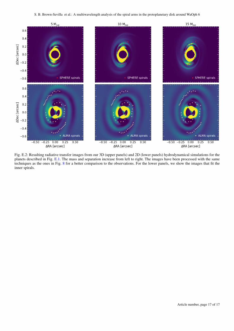
S. B. Brown-Sevilla et al.: A multiwavelength analysis of the spiral arms in the protoplanetary disk around WaOph 6
Fig. E.2: Resulting radiative transfer images from our 3D (upper panels) and 2D (lower panels) hydrodynamical simulations for theplanets described in Fig. E.1. The mass and separation increase from left to right. The images have been processed with the sametechniques as the ones in Fig. 8 for a better comparison to the observations. For the lower panels, we show the images that fit theinner spirals.
Article number, page 17 of 17