Brett A. Bednarcyk and Steven M. ArnoldGlenn Research Center, Cleveland, Ohio

A Multiscale, Nonlinear, Modeling Framework Enabling the Design and Analysis of Composite Materials and Structures

NASA/TM—2012-217244

February 2012

https://ntrs.nasa.gov/search.jsp?R=20120014088 2018-07-13T12:53:01+00:00Z

NASA STI Program . . . in Profile

Since its founding, NASA has been dedicated to the advancement of aeronautics and space science. The NASA Scientific and Technical Information (STI) program plays a key part in helping NASA maintain this important role.

The NASA STI Program operates under the auspices of the Agency Chief Information Officer. It collects, organizes, provides for archiving, and disseminates NASA’s STI. The NASA STI program provides access to the NASA Aeronautics and Space Database and its public interface, the NASA Technical Reports Server, thus providing one of the largest collections of aeronautical and space science STI in the world. Results are published in both non-NASA channels and by NASA in the NASA STI Report Series, which includes the following report types: • TECHNICAL PUBLICATION. Reports of

completed research or a major significant phase of research that present the results of NASA programs and include extensive data or theoretical analysis. Includes compilations of significant scientific and technical data and information deemed to be of continuing reference value. NASA counterpart of peer-reviewed formal professional papers but has less stringent limitations on manuscript length and extent of graphic presentations.

• TECHNICAL MEMORANDUM. Scientific

and technical findings that are preliminary or of specialized interest, e.g., quick release reports, working papers, and bibliographies that contain minimal annotation. Does not contain extensive analysis.

• CONTRACTOR REPORT. Scientific and

technical findings by NASA-sponsored contractors and grantees.

• CONFERENCE PUBLICATION. Collected papers from scientific and technical conferences, symposia, seminars, or other meetings sponsored or cosponsored by NASA.

• SPECIAL PUBLICATION. Scientific,

technical, or historical information from NASA programs, projects, and missions, often concerned with subjects having substantial public interest.

• TECHNICAL TRANSLATION. English-

language translations of foreign scientific and technical material pertinent to NASA’s mission.

Specialized services also include creating custom thesauri, building customized databases, organizing and publishing research results.

For more information about the NASA STI program, see the following:

• Access the NASA STI program home page at http://www.sti.nasa.gov

• E-mail your question via the Internet to help@

sti.nasa.gov • Fax your question to the NASA STI Help Desk

at 443–757–5803 • Telephone the NASA STI Help Desk at 443–757–5802 • Write to:

NASA Center for AeroSpace Information (CASI) 7115 Standard Drive Hanover, MD 21076–1320

Brett A. Bednarcyk and Steven M. ArnoldGlenn Research Center, Cleveland, Ohio

A Multiscale, Nonlinear, Modeling Framework Enabling the Design and Analysis of Composite Materials and Structures

NASA/TM—2012-217244

February 2012

National Aeronautics andSpace Administration

Glenn Research Center Cleveland, Ohio 44135

Acknowledgments

The authors acknowledge the efforts of NASA GSRP Fellows K.C. Liu and John Hutchins who contributed to the models and results presented herein.

Available from

NASA Center for Aerospace Information7115 Standard DriveHanover, MD 21076–1320

National Technical Information Service5301 Shawnee Road

Alexandria, VA 22312

Available electronically at http://www.sti.nasa.gov

Level of Review: This material has been technically reviewed by technical management.

Trade names and trademarks are used in this report for identification only. Their usage does not constitute an official endorsement, either expressed or implied, by the National Aeronautics and

Space Administration.

NASA/TM—2012-217244 1

A Multiscale, Nonlinear, Modeling Framework Enabling the Design and Analysis of Composite Materials and Structures

Brett A. Bednarcyk and Steven M. Arnold

National Aeronautics and Space Administration Glenn Research Center Cleveland, Ohio 44135

Abstract A framework for the multiscale design and analysis of composite materials and structures is

presented. The ImMAC software suite, developed at NASA Glenn Research Center, embeds efficient, nonlinear micromechanics capabilities within higher scale structural analysis methods such as finite element analysis. The result is an integrated, multiscale tool that relates global loading to the constituent scale, captures nonlinearities at this scale, and homogenizes local nonlinearities to predict their effects at the structural scale. Example applications of the multiscale framework are presented for the stochastic progressive failure of a SiC/Ti composite tensile specimen and the effects of microstructural variations on the nonlinear response of woven polymer matrix composites.

Introduction The use of advanced composites (polymer matrix composites (PMCs), ceramic matrix composites

(CMCs), and metal matrix composites (MMCs)) provides benefits in the design of advanced lightweight, high temperature, structural systems by providing an increase in specific properties (e.g., strength to density ratio) when compared to their monolithic counterparts. To fully realize the benefits offered by these materials, however, experimentally validated, computationally efficient, multiscale design and analysis tools must be developed for the advanced, multiphased materials of interest. Furthermore, in order to assist both the structural analyst in designing with these materials and the materials scientist in designing/developing the materials, these tools must encompass the various levels of scale for composite analysis as illustrated in Figure 1.

These scales are the micro scale (constituent level), the mesoscale (laminate/composite and/or stiffened panel level) and the macro scale (global/structure level), and they progress from left to right in Figure 1. One traverses these scales using homogenization (moves right) and localization (moves left) techniques, respectively (Figure 2 and Figure 3); where a homogenization technique provides the properties or response of a “structure” (higher level) given the properties or response of the structure’s “constituents” (lower scale). Conversely, localization techniques provide the response of the constituents given the response of the structure. Figure 3 illustrates the interaction of homogenization and localization techniques, in that during a multi-scale analysis, a particular stage in the analysis procedure can function on both levels simultaneously. For example, in Figure 3, the constituents X and Y at Level 1, when combined (homogenized) become the constituent V (on Level 2) which is subsequently combined with W to produce U (the effective structure at Level 3). The reverse process is known as localization, in which the constituent level responses (Level 1) are determined from the structure level (Level 3) results. Obviously, the ability to homogenize and localize accurately requires a sophisticated theory that relates the geometric and material characteristics of structure and constituents.

Additionally, Figure 3 illustrates that experiments (virtual or laboratory) performed at each level can be viewed either as exploratory or characterization experiments used to obtain the necessary model parameters for the next higher level. Alternatively, these tests can be viewed as/used to validate the modeling methods employed at the lower level. Figure 3 also illustrates the authors’ view that the term “multiscale modeling” should imply consideration of at least two levels of homogenization/localization or a minimum of three levels of scale. The rationale is that if analyses that consider only two levels of scale

NASA/TM—2012-217244 2

Figure 1.—Illustration of associated levels of scale for multiscale composite analysis.

Figure 2.—Homogenization provides the ability to

determine structure level properties from constituent level properties while localization provides the ability to determine constituent level responses from structure level results.

Figure 3.—Multilevel tree diagram illustrating three levels of scale and

the role of testing for both validation and characterization. (rather than two homogenizations) are considered to be multiscale, many standard structural analyses would qualify. For instance, an elastic finite element model of a structure considers the materials with given elastic properties as Level 1 and the structural response as Level 2. Similarly, standard classical lamination theory considers the plies (with given elastic properties) as Level 1 and the laminate (with calculated ABD stiffness matrix) as Level 2. It is our position that the term “multiscale modeling” is intended to distinguish an analysis from such standard analyses that consider only two scales. Examining the recent literature in multiscale modeling revealed that a majority of authors have not applied this standard to their own work, as evidenced by the fact that 66 percent of the papers that were characterized by the authors as involving multiscale modeling considered only two scales (Ref. 1).

NASA/TM—2012-217244 3

Numerous homogenization techniques (micromechanical models) exist that can provide effective composite properties. These range from the simplest, analytical approximations (i.e., Voigt/Reuss) to higher fidelity, more involved methods (e.g., concentric cylinder assemblage, Mori-Tanaka, Eshelby, and Aboudi’s generalized method of cells) to finally, fully numerical methods that are the most general and the highest fidelity yet the most computationally intense (e.g., finite element, boundary element, Fourier series). Each has its realm of applicability and advantages, however, many are unable to admit general user defined deformation and damage/failure constitutive models for the various constituents (i.e., fiber or matrix) thus limiting their ultimate usefulness, especially for high temperature analysis where nonlinear, time-dependent behavior is often exhibited.

An alternative approach to modeling composite structures, which circumvents the need for micromechanics, involves fully characterizing the composite material or laminate experimentally, which has the advantage of capturing the in-situ response of the constituents perfectly. However, such full characterization for all applicable temperatures and configurations (e.g., fiber volume fractions, tow spacing’s, etc.) can be expensive. In addition, composites are almost always anisotropic on this scale (i.e., laminate). Thus some needed properties can be virtually impossible to measure, and the development of realistic models that capture the nonlinear, multiaxial deformation and failure can be challenging (due to the anisotropy). Clearly, the physics of deformation and failure occur on the micro scale (and below), and, by modeling the physics at the micro scale, models for the monolithic, often isotropic, constituents can be employed.

Recently, a comprehensive and versatile micromechanics analysis computer code, known as MAC/GMC (Ref. 2) has been developed at NASA Glenn Research Center based on Aboudi’s well-known micromechanics theories (Refs. 3 to 6). FEAMAC (the coupling of MAC/GMC micromechanics with the finite element analysis framework through user subroutines), HyperMAC (the coupling of MAC/GMC micromechanics with the commercial structural sizing software known as HyperSizer (Ref. 7)), and Multiscale Generalized Method of Cells (MSGMC, the recursive coupling of micromechanics with micromechanics) have begun to address the truly multiscale framework depicted in Figure 1. This software suite, known collectively as ImMAC (available from NASA Glenn), provides a wide range of capabilities for modeling continuous, discontinuous, woven, and smart (piezo-electo-magnetic) composites. Libraries of nonlinear deformation, damage, failure, and fiber/matrix debonding models, continuous and discontinuous repeating unit cells (RUCs), and material properties are provided. To illustrate the multiscale capabilities of the ImMAC framework, this paper focuses on the application of FEAMAC and MSGMC to model the stochastic progressive failure of a SiC/Ti metal matrix composite tensile specimen and to investigate architectural variability on the nonlinear response of woven PMCs.

FEAMAC As shown in Figure 4(a), FEAMAC is the direct implementation of MAC/GMC unit cell analyses

within structural finite element analysis (FEA). The software currently supports Simulia’s commercial finite element software package Abaqus (Ref. 8). The coupling is accomplished utilizing the Abaqus user subroutines, which enable the MAC/GMC code to be called as a library to represent the composite material response at the integration and section (used for through-thickness integration in shell elements) points in any element within the finite element model. Two- and three-dimensional continuum elements, as well as shell elements, are supported. Any nonlinearities due to local effects (e.g., inelasticity or damage) in the fiber/matrix constituents at any point in the structure are thus captured and homogenized, and their effects on the structure are manifested in the finite element model structural response at each increment of loading.

NASA/TM—2012-217244 4

(a) (b) Figure 4.—(a) FEAMAC couples MAC/GMC with finite element analysis. (b)MSGMC recursively calls

the generalized method of cells (GMC) to represent the behavior within the subcells of a RUC operating at a given level.

MSGMC As shown in Figure 4(b), MSGMC (Ref. 9) implements the three-dimensional generalized method of

cells (GMC) to represent the behavior of the subcells within GMC repeating unit cells. This can be performed an arbitrary number of times to represent an arbitrary number of scales in an integrated multiscale analysis. The methodology is ideal for analyzing woven and braided composites, where the behavior of the tows can be modeled with GMC operating within a subcell in an RUC representing the weave or braid. Similar to FEAMAC, any nonlinearity occurring at the lower scales will affect the global scale response.

Results and Discussion Progressive Failure Analysis of a SiC/Ti Tensile Specimen

The stochastic analysis of the fiber breakage dominated progressive failure process in a longitudinally-reinforced SiC/Ti MMC structures is examined using FEAMAC. In particular, we consider perhaps the simplest (yet extremely important) composite structure: an experimental tensile test specimen, shown in Figure 5. Such test specimens are critical to both materials scientists and structural engineers because they are used to evaluate material quality during development of materials and to characterize material model parameters needed for structural analysis. The design of test specimens is also known to be critical so as to ensure a uniform state of stress and strain in the gauge section, as well as consistent failure within the gauge section.

NASA/TM—2012-217244 5

Figure 5.—NASA Glenn dog-bone test specimen.

Figure 6.—Abaqus finite element mesh of the dogbone specimen and MAC/GMC RUC operating at

each integration point.

The SiC/Ti test specimen was modeled with a one-eighth symmetry finite element mesh. A monotonic longitudinal tensile load was applied in the form of an applied uniform displacement in the direction of the longitudinal axis (x1) of the specimen at a rate of 3×10-4 in./s. With a total of 300 Abaqus C3D8 (8-noded brick) elements in the mesh and eight integration points per element, the MAC/GMC micromechanics model is called as a user material (UMAT) subroutine 2400 times per time step in the FEAMAC simulation. This highlights the necessity for having such a computationally-efficient means as GMC of relating both the properties and the local stress/strain fields of the constituent phases of the composite to the effective properties and deformation response of its homogenized continuum representation. Note that, based on the mesh shown in Figure 6, along with the fiber diameter and composite fiber volume fraction, each element in the tensile specimen gauge section is sufficiently large to encompass approximately 25 fibers.

On the local scale within the MAC/GMC input files, which define the composite material details, in addition to the geometry of the composite RUC, material properties for the fiber and matrix are required. The SiC fiber is treated as linearly elastic and isotropic while the TIMETAL 21S matrix is treated as viscoplastic and was simulated using the Generalized Viscoplasticity with Potential Structure (GVIPS) constitutive model (Ref. 10). The material properties of the constituents are given in Table 1 and Table 2.

TABLE 1.—SCS-6 FIBER ELASTIC PROPERTIES Temperature

(°C) E

(GPa) ν α

(1×10-6/°C) 21 393 0.25 3.56

316 382 0.25 3.72 427 378 0.25 3.91 538 374 0.25 4.07 860 368 0.25 4.57

NASA/TM—2012-217244 6

TABLE 2.—TIMETAL 21S MATERIAL PROPERTIES AND GVIPS MODEL PARAMETERS Temperature

(°C) E

(GPa) α

(1×10-6/°C) κ

(MPa) µ

(MPa/s) B0

(MPa) Rα

(1/s) β

23 114.1 7.717 1029 667.6 6.908×10-5 0 0.001 300 107.9 9.209 768.4 137.8 1.035×10-4 0 0 500 95.1 10.70 254.2 1.45×10-3 2.756×10-4 1.68×10-7 0 650 80.7 12.13 5.861 6.19×10-9 5.870×10-4 1.00×10-6 0 704 59.7 14.09 0.756 1.13×10-11 6.346×10-4 6.01×10-5 0

Temperature-independent: ν = 0.365, n = 3.3, B1 = 0.0235, p = 1.8, q = 1.35 The final ingredient to the multiscale FEAMAC progressive failure analysis of the TMC specimen is

the stochastic failure response of the SiC fibers, as shown in Figure 7. Two approaches to modeling this stochastic behavior will be investigated and compared. The first relies on the stochastic Curtin fiber failure model (Ref. 11) and the second is based on a simple maximum stress failure criterion, which is deterministic when applied uniformly across the test specimen and stochastic when the strength is randomly distributed throughout the specimen. Both failure models are applicable only to the fiber subcell(s) within the RUC. The Curtin model predicts fiber stiffness degradation due to damage and complete failure of an effective, degrading fiber. Herein, upon complete failure using either the Curtin or maximum stress model, the fiber is given a negligible stiffness (0.0001 times its original stiffness). The employed Curtin model parameters (which are obtained from fiber strength statistics, see Figure 7) are the fiber gauge length, L0 = 1 in. (25.4 mm), fiber diameter, d = 0.0056 in. (142 µm), characteristic strength, σ0 = 609 ksi (4200 MPa), Weibull modulus, m = 10. The Curtin model requires one additional parameter, the fiber-matrix frictional sliding resistance, τ, which was taken as τ = 2.03 ksi (14 MPa) at 650 °C based on the work described in (Ref. 12). This value was backed out of GMC simulations such that good correlation was achieved with test data. Thus, because these simulations were based on GMC simulations for a single material point at a specific temperature, the applicability of this τ value in the simulations of the entire tensile specimen and at temperatures other than 650 °C is questionable.

First let us consider a simulation with no fiber failure as shown in Figure 8(a). The plotted von Mises stress field shows the stress concentrations that are inherent to dogbone type test specimens. Along the specimen edge, a strong minimum is observed at the start of the reduction section, whereas a milder maximum is present at the transition from the reduction section to the gauge section. Because it is relatively mild, this maximum is difficult to see in the figure, but as indicated, it is an absolute maximum at node 67, which is just above the transition to the gauge section. It is this structural level concentration that can lead to specimen failure outside the gauge section, which is why a large reduction radius (14.5 in.) was employed in the NASA Glenn specimen, thus making this concentration very mild. It has been shown that for smaller reduction radii, this concentration increases significantly (Refs. 13 and 14). Even though the magnitude of this stress riser, as modeled, is only slightly higher than the stress magnitude in the gauge section, this will always be the location of simulated failure initiation if the fiber failure parameters are spatially uniform throughout the tensile specimen.

The effect of the global stress riser can be seen in Figure 8(b) and (c), where the fiber damage progression is shown for the max stress and Curtin model simulations. Note that the fiber damage is quantified as a fraction of fiber damage within the elements; a fiber damage value of zero corresponds to an undamaged state, while a fiber damage value of 1.00 corresponds to complete failure of all fibers within an element. For the case in which we use the maximum stress criterion, the failure simulation is fully deterministic as fiber failure initiates at the stress riser and no statistical data related to the fiber strength are employed. If one uses the Curtin model, failure still initiates at the highest global stress raiser, but now the stochastic nature of the fiber failure process is captured at the local level through the fiber strength statistics incorporated within the model. Both fiber failure models exhibit similar damage zones and both simulations exhibit complete failure of the specimen within 1/10,000th of a second after initiation

NASA/TM—2012-217244 7

of failure begins. This is despite the fact that the Curtin model simulates fiber stiffness degradation prior to failure while the max stress model does not. The Curtin model simulation does fail at a significantly lower overall stress than does that using the maximum stress criterion; see the composite stress-strain curves in Figure 9. However, these results are dependent on the chosen value of τ, the fiber-matrix frictional sliding resistance. A higher value of τ would shift the Curtin model failure predictions higher, closer to those of the max stress criterion. Note, the strain plotted in Figure 9 corresponds to a virtual extensometer measurement, that is, an average strain over the gauge length of the specimen as shown in Figure 8(c) (calculated as change in displacement divided by original length).

Figure 7.—Fiber strength histogram for SCS-6 SiC fibers. The actual data is

vendor-supplied (Ref. 15), while the simulated data refers to the distributed characteristic strength. Note, the fiber gauge length: L0 = 1 in. (25.4 mm) and diameter: d = 0.0056 in. (142 µm) are vendor supplied.

Figure 8.—(a) Stress contours in the longitudinal 33 percent SiC/Ti-21S tensile specimen in a linear elastic

simulation with no fiber failure indicating the maximum stress riser at node 67. Local fiber damage fraction as a function of time as fiber failure progresses within the longitudinal 33 percent SiC/Ti-21S specimen with spatially uniform fiber failure model parameters. (b) Max stress criterion. (c) Curtin model.

0.00

0.05

0.10

0.15

0.20

0.25

0.30

150 200 250 300 350 400 450 500 550 600 650 700 750 800 850Fiber Strength (ksi)

Freq

uenc

y

ActualSimulated (30 Bins)

(a) (b) (c)

NASA/TM—2012-217244 8

Figure 9.—Stress-strain curves assuming both spatially uniform and spatially

random failure strengths for unidirectional, 33 percent fiber volume fraction, SiC/Ti21S composite specimen.

At this point it is worthwhile to summarize the process involved in the FEAMAC simulation results (see for example Figure 8 and Figure 10). Global incremental displacement loading is applied on the specimen, and Abaqus solves the structural problem to determine the stress and strain fields throughout the specimen. The strains and strain increments at each integration point are then passed to MAC/GMC (through the Abaqus UMAT subroutine), which performs a micromechanics analysis given the composite local geometry and constituent properties. Within MAC/GMC, the integration point strains are localized to the level of the fiber and matrix constituent subcells (see Figure 6), which allows determination of the viscoplastic behavior of the matrix and the damage/failure behavior of the fiber. The local response of the fiber and matrix subcells are then homogenized within MAC/GMC to obtain new stresses and a new stiffness matrix (which may have changed due to the imposed strain increment and additional damage accumulation) for the composite at each particular integration point. This information is passed back to Abaqus (through the UMAT subroutine), which then imposes the next increment of the applied global loading. This multiscale approach enables the effects of damage, failure, and inelasticity, and the associated redistribution of stresses within the RUC, to impact the global specimen response. When a particular integration point experiences fiber failure its stiffness is significantly reduced, which causes it to shed load to the surrounding integration points that remain intact and may cause failure to progress, as shown in Figure 8. It should be noted that complete fiber failure through the specimen, as depicted in Figure 8, does not truly represent complete separation in the simulation because matrix material subcells remain intact within the RUCs (see Figure 6). A matrix failure criterion could be added to the simulation within MAC/GMC to model complete failure. However, since the tensile failure of longitudinal SiC/Ti specimens is known to be dominated by fiber failure, this was not done here as the current results are expected to be representative.

It is clear from Figure 8 that the multiscale stochastic FEAMAC simulation of the SiC/Ti specimen has predicted failure outside of the gauge section, which does not typically occur with the NASA Glenn MMC tensile specimen. This shortcoming is due to the inappropriate implementation of the fiber strength variability exclusively at the local level (i.e., uniform spatial variation of strength). In order to more realistically simulate the SiC/Ti tensile specimen progressive failure, it is necessary to account for the

0

50

100

150

200

250

300

350

0.000 0.003 0.006 0.009 0.012 0.015 0.018

Stre

ss (k

si)

Strain

Spatially Uniform - Max Stress (2x2)

Spatially Uniform - Curtin (2x2)

Global Distribution - Max Stress (2x2)

Global Distribution - Curtin (2x2)

NASA/TM—2012-217244 9

realistic fiber strength distribution on the structural level. This was accomplished by varying the max stress criterion in one case and the Curtin model parameters (an obvious choice being the characteristic strength, σ0) in the other case, over the specimen geometry. Providing different elements with different values of these model parameters, in essence, enables the elements to damage and fail at different local fiber stress levels.

To distribute the characteristic strength spatially, 30 user materials were associated with the finite element mesh of the composite specimen. Each material was defined by a MAC/GMC input file with a different σ0 value chosen according to the vendor-supplied fiber strength histogram shown in Figure 7. This was accomplished by determining the number of user materials having σ0 values in each 50 ksi range (see the horizontal axis of Figure 7) in order to provide a good match with the actual fiber strength distribution (as shown in Figure 7). If only one material’s σ0 value was located within a particular 50 ksi range, the characteristic strength was chosen as the middle of that range. Otherwise, the characteristic strength values for the materials were evenly distributed within the applicable 50 ksi range. As shown in Figure 7, the 30 σ0 values provide an excellent match with the actual fiber strength histogram. When considering the Curtin model, the other important parameter that must be considered to obtain the correct fiber strength statistics is the Weibull modulus, m, as this affects the shape of the fiber strength distribution. Immediately, one might consider using a constant value of m for all values of σ0, yet when summing over all fibers, this did not reproduce the correct overall fiber strength distribution. If however, each user material was allowed to have a distinct Weibull modulus value, one could obtain the correct distribution. Consequently, a simple computer program was written to optimize the Weibull modulus values in order to provide the best correlation of the combined fiber strength distribution of all 30 user materials with the actual fiber strength distribution.

Now, with these 30 user materials (represented by 30 MAC/GMC input files) whose Curtin model data (or maximum strength criterion data, depending upon which failure model one chooses to employ) cumulatively represent the fiber strength statistics accurately, the 300 elements within the specimen were randomly distributed to the user materials (with ten elements per material, all ten having identical properties). The random distribution was accomplished via a simple computer program. The resulting distribution of maximum characteristic strengths (i.e., σ0) over the specimen geometry is shown in Figure 10 (left most figure). This idealization (i.e. spatially varying fiber strength distribution) was subjected to the identical simulated tensile test considered previously in the non-distributed case. Results for the progressive failure simulation of the spatially distributed maximum fiber strength statistics specimen are given in Figure 10. In this simulation, failure initiated (see Figure 10 snapshot (a)) not at the stress concentration (i.e., node 67, see Figure 8(a)), but rather within the gauge section in an element that happened to be assigned a low characteristic strength (see the blue element in the left most Figure 10). Subsequently, progressive failure across the specimen occurred in 0.68 s (see snapshots (b) through (e) in Figure 10). The global stress-strain curve responses for the both the Curtin and maximum stress model predictions are shown in Figure 9 for both uniform and spatially varying cases. Clearly, the peak stress value (ultimate strength) in both of these predicted stress-strain curves are significantly lower than the previous uniformly (or non-distributed) case; in that the distributed Curtain model simulation predicts an ultimate strength of 210 ksi (1451 MPa) compared to a value of 264 ksi (1822 MPa) for the non-distributed simulation, while the maximum stress criterion simulation predicts, an ultimate strength of 217 ksi (1494 MPa) compared to a value of 313 ksi (2155 MPa) for the non-distributed simulation. Note how both spatially distributed simulations, regardless of the failure model used, provide similar (less than 3 percent difference) results; as both are now stochastic in nature due to the random spatial variation of fiber strength. Furthermore, random failure locations within the gauge length can be obtained by creating different actualizations (i.e., new random assignments of fiber strengths within the various 30 bins); which agrees qualitatively with numerous experimental results obtained at NASA Glenn as shown in Figure 11.

NASA/TM—2012-217244 10

Figure 10.—Global fiber strength distribution contour

plot; (a) to (e) cumulative fiber subcell failure contours at simulation times of 63.40, 63.93, 63.95, 64.06, and 64.08 s, respectively (Note that the black lines denote the beginning of the transition region from the end of the gage section to the end of the specimen).

Figure 11.—(a) Picture of the failure location of six test specimens and (b) to (g) Cumulative fiber

subcell failure contour plots showing probabilistic nature of the simulated fiber failure location from six separate actualizations (simulations). Note that the black lines denote the beginning of the transition region from the end of the gage section to the end of the specimen once again.

(a)

(b) (c) (d) (e) (f) (g)

σ0 (ksi)

NASA/TM—2012-217244 11

To assess the quantitative accuracy via comparison with experimental results, three additional factors are accounted for in the FEAMAC simulation: (1) local fiber strength variation within the RUC, (2) incorporation of residual stresses due to specimen heat treatment/consolidation, and (3) shifted fiber strength due to fiber length scale. In order to account for the local fiber strength distribution within the RUC, an RUC containing 25 subcells (see insert in Figure 12) was utilized. Furthermore each fiber subcell was randomly assigned a different strength while maintaining that the average of these fiber strengths equals the specific fiber strength assigned to the RUC. Recall that the 30 RUCs (10 elements per RUC) are randomly assigned throughout the 300 element mesh in order to capture the global fiber strength distribution. This enables each integration point to experience a progressive failure which in turn enables an even more gradual failure evolution than if one utilizes only a global fiber strength distribution, with one fiber per RUC at an integration point. Incorporation of residual stresses (which are key for accurate predictions of metal matrix composites failure response) is accomplished by imposing the complete thermomechanical loading cycle for a given specimen. A 16 hr cool down from a uniform 900 °C (assumed stress-free) heat treatment temperature to room temperature (23 °C), was simulated followed by an unconstrained temperature rise to 650 °C over 5 min. The temperature was then held constant while a monotonic uniaxial tensile loading, at a displacement rate of 3×10-4 in/s, was applied until complete fiber failure was achieved. The predicted tensile response of a 25 percent fiber volume fraction SiC/Ti titanium matrix composite (TMC) test specimen at 650 °C is shown in Figure 12, given the vendor supplied strength distribution of Figure 7, which is also shown as the black line (λ = 1.0) in the insert of Figure 12. Clearly, this curve agrees well with the experimental data provided, except it appears to suffer premature fiber failure since it significantly under predicts the specimen UTS.

To compensate for this premature failure, we must account for the disparity between the gage length of the fiber specimens used to conduct the fiber strength tests (L0 = 1.0 in) and the characteristic length needed to develop full fiber loading in the FE model (calculated to be L= 0.091 in. from shear-lag

Figure 12.—Composite stress-strain response for randomly distributed, maximum stress

failure criterion simulations (black and blue lines) compared to experimental data (red square symbols) at 650 °C.

NASA/TM—2012-217244 12

calculations (Refs. 16 and 17)). Consequently, a new set of fiber strength bins were generated using a modified Weibull distribution, shifted to account for this change in length ratio (this ratio is defined as lambda, or L/L0 (Ref. 11)):

( )

σσ

−−=σm

f LLp

00exp1 (1)

The original and shifted Weibull distributions (failure probability distribution) are illustrated in the lower right insert in Figure 12. These new fiber strength RUCs were then used to simulate the same thermomechanical loading cycle described previously, the result of which is depicted by the blue line in Figure 12. Clearly, this new simulation captures the experimental data response extremely well including the UTS of this test. Note however, that the strain to failure is over predicted; as expected since no failure criterion was applied to the matrix subcells, so that upon complete failure of the fiber subcells matrix inelastic flow is unconstrained.

Recursive Multiscale Analysis of a Woven Polymer Matrix Composite

In this study, MSGMC is used to examine the effects of architectural parameter variations on the response of woven PMCs. As illustrated in Figure 13, the analysis considers four physical length scales from the fiber/matrix constituents (microscale) to the RUC representing the tow (mesoscale) to the RUC of the weave (macroscale) to an assembly of nine RUCs (structural scale). This would normally indicate three separate homogenizations to span the four scales, but actually, an additional intermediate homogenization is performed when using MSGMC to analyze woven or braided composites. This involves a separate through-thickness homogenization within the macroscale, which has been shown to improve the model’s predictions (see Ref. 19 for details). Thus, the analyses at the structural scale involve four homogenizations while those at the macroscale involve three. The architectural parameters that were varied at the mesoscale (fiber packing arrangement and fiber volume fraction within the tows) and the macroscale (tow aspect ratio) are also shown in Figure 13.

For these analyses an AS-4/3501-6 material system with an overall fiber volume fraction of 60 percent was assumed. The properties of the constituent materials are shown in Table 3. The fiber is treated as linearly elastic while the matrix is modeled as elastoplastic using classical plasticity with exponential isotropic hardening of the form,

( ) ( )e 1pAp Y

HA

− εκ ε = σ − − (2)

where ( )pκ ε is the isotropic strain hardening rule, pε is the equivalent plastic strain, and the material

parameters are σY (yield strength), H (initial post-yield modulus), and A (exponent) (see Ref. 20 for details). To study the effects of architectural and material variation on the macroscale response, a full factorial set of numerical simulations were conducted. The parameters varied are shown in Table 4 and are depicted in Figure 13. The three architectural parameters varied are tow volume fraction, tow aspect ratio (width divided by thickness, as shown in Figure 13) and fiber packing arrangement. All other parameters in the analysis were kept constant. The tow volume fraction and fiber packing arrangement are both considered mesoscale attributes because their geometrical properties are involved in the mesoscale concentration matrix. The tow aspect ratio is considered a macroscale property because it is taken into account in the macroscale concentration matrices. The tow volume fraction was varied among 0.62, 0.65, and 0.70. These three values were chosen based on common experimental values for PMCs. The tow aspect ratio was chosen to be 9, 18, or 36. A value of 9 is typical of CMCs, 18 is typical of PMCs, and 36 was chosen as an upper bound. Two different fiber packing arrangements were considered, square and hexagonal, as both exhibit different responses. Although most PMCs exhibit random packing, square and

NASA/TM—2012-217244 13

TABLE 3.—AS-4/3501-6 CONSTITUENT PROPERTIES

EA (GPa)

ET (GPa)

vA vT GA (GPa)

σY (MPa)

a H (GPa)

AS-4 225.0 15.0 0.2 0.2 15.0 N/A N/A N/A 3501-6 4.2 4.2 0.34 0.34 1.56 71 100 1.5

TABLE 4.—PARAMETERS VARIED IN MULTISCALE ANALYSES

Microstructural parameter Relevant length scale Values Tow volume fraction (Vtf) Meso 0.62, 0.65, 0.70 Tow packing Meso Hexagonal, Square Tow aspect ratio (AR) Macro 9, 18, 36

Figure 13.—Multiscale analysis methodology with architectural effects being varied as

shown at the meso and macroscales.

(a) (b) Figure 14.—Weave macroscale RUCs, (a) plain and (b) 5HS.

hexagonal packing are both reasonable approximations of this. The full factorial simulations were executed for both the tension and shear response and were also performed for two macroscale weave types: plain weave and 5-harness satin (5HS) weave (see Figure 14). The full factorial simulations for both responses and weave types resulted in a total of 72 cases analyzed. In each of these cases, the overall volume fraction of the woven composite was kept constant so that the results are comparable.

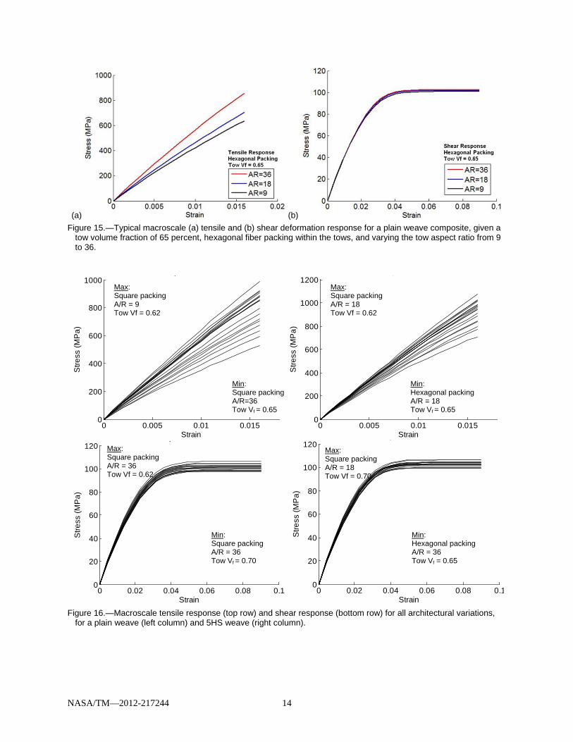
The typical simulated stress-strain curves for a plain weave composite subjected to tensile and shear loading are shown in Figure 15, where a single RUC of the composite (i.e., macro response) has been considered. For illustrative purposes, only one architectural parameter, namely, the tow aspect ratio, was varied. Clearly this variation has a significant effect on the macroscale tensile response, but little effect on the shear response. The full factorial parameter variation results for the macroscale analyses are presented in Figure 16, with each curve on each chart representing a particular set of architectural parameters. It is apparent that there is a significant amount of variation at the macroscale caused by varying the architectural parameters even though the overall fiber volume fraction of the composite is kept constant. The architectural parameter variation caused approximately three times more macroscale variation in the

NASA/TM—2012-217244 14

(a) (b) Figure 15.—Typical macroscale (a) tensile and (b) shear deformation response for a plain weave composite, given a

tow volume fraction of 65 percent, hexagonal fiber packing within the tows, and varying the tow aspect ratio from 9 to 36.

Figure 16.—Macroscale tensile response (top row) and shear response (bottom row) for all architectural variations,

for a plain weave (left column) and 5HS weave (right column).

0 0.005 0.01 0.0150

200

400

600

800

1000

Strain

Stre

ss (M

Pa)

p

0 0.005 0.01 0.0150

200

400

600

800

1000

1200

Strain

Stre

ss (M

Pa)

p

0 0.02 0.04 0.06 0.08 0.10

20

40

60

80

100

120

Strain

Stre

ss (M

Pa)

p

0 0.02 0.04 0.06 0.08 0.10

20

40

60

80

100

120

Strain

Stre

ss (M

Pa)

p

Min: Square packing A/R = 36 Tow Vf = 0.70

Min: Hexagonal packing A/R = 36 Tow Vf = 0.65

Max: Square packing A/R = 9 Tow Vf = 0.62

Min: Square packing A/R=36 Tow Vf = 0.65

Max: Square packing A/R = 18 Tow Vf = 0.62

Min: Hexagonal packing A/R = 18 Tow Vf = 0.65

Max: Square packing A/R = 36 Tow Vf = 0.62

Max: Square packing A/R = 18 Tow Vf = 0.70

NASA/TM—2012-217244 15

composite tensile response compared to the shear response (as measured by standard deviation). However, the variation in the shear stress-strain curves was still appreciable. Further, examination of individual stress-strain curves revealed that decreasing tow volume fraction has the same effect as increasing tow aspect ratio, an increase in modulus and strain energy (area under stress-strain curve). Also, the hexagonal RUC at the mesoscale was more compliant and exhibited more plasticity than the square RUC for equivalent volume fractions.

To examine the structural scale, the effects of parameter variation on the response of nine (3×3) macroscale RUCs was studied (see Figure 13). Each of the RUCs composing the 3×3 RUC at the structural scale is comprised of a macroscale RUC with a set of architectural parameters chosen at random from the permutations considered in the macroscale architectural study. For example, one RUC might have a 62 percent tow volume fraction with an aspect ratio of 18 and square packing and another could be completely different. Each architectural parameter was randomly selected for each RUC, without imposing any probabilities on the parameters. Thirteen cases (realizations) were run for each structural RUC in order to achieve a broad spectrum of combinations. The results for all 13 cases are shown in Figure 17. It is important to note that the variance is greatly reduced when compared to that observed in the macroscale plots. The maximum standard deviation at the macroscale was 15 percent compared to a mere 2 percent at the structural scale, Consequently, it appears that the effects of lower scale variations are diminished after one or two higher length scales of homogenization. Thus one must be cautious in attempting to draw conclusions regarding the impact of variability observed at a given scale on the behavior at higher scales.

Figure 17.—Structural (3x3 RUCs) tensile response (top row) and shear response (bottom row) for all

architectural variations, for a plain weave (left column) and 5HS weave (right column).

0 0.005 0.01 0.0150

100

200

300

400

500

600

700

800

Strain

Stre

ss (M

Pa)

p

0 0.005 0.01 0.0150

100

200

300

400

500

600

700

800

900

Strain

Stre

ss (M

Pa)

p

0 0.01 0.02 0.03 0.04 0.05 0.060

20

40

60

80

100

Strain

Stre

ss (M

Pa)

p

0 0.01 0.02 0.03 0.04 0.05 0.060

20

40

60

80

100

Strain

Stre

ss (M

Pa)

p

NASA/TM—2012-217244 16

Conclusions NASA Glenn Research Center’s ImMAC software suite provides an integrated multiscale framework

for the design and analysis of composite materials and structures. FEAMAC calls the GMC micromechanics methods to represent the nonlinear composite constitutive response at the integration points (and section points) within an Abaqus finite element analysis. MSGMC calls GMC micromechanics recursively such that at any scale, the GMC subcells may be occupied by an effective composite material. GMC’s ability to localize and homogenize extremely efficiently enables these types of integrated multiscale analyses where nonlinear deformation and damage models for the constituents drive the nonlinear response at the structural scale. Furthermore, because the nonlinear deformation and damage is handled at the constituent scale, complex, multiaxial, anisotropic models, which would be needed at the composite scale, can be avoided.

Examining the response of a SiC/Ti tensile specimen using FEAMAC, it was shown that incorporating stochastic features at the proper scale (spatially random at the local/global level) enables the use of a simple failure model (e.g., max stress criterion). The model was shown to predict realistic gauge section failure and accurate deformation response and failure load level in the specimen. MSGMC was used to model the nonlinear deformation response plain weave and 5-harness satin graphite/epoxy composites. The effects of tow fiber volume fraction, tow fiber packing arrangement, and tow aspect ratio were shown to be significant when examining the nonlinear response of a single RUC. However, when the response of a structure (idealized with nine RUCs) is modeled, the effects of such variations are greatly reduced. It is also noteworthy that the presented structural MSGMC simulations involve four homogenizations across five levels of scale.

References 1. Sullivan, R.W. and Arnold, S.M., “An Annotative Review of the Experimental & Analytical

Requirements to Bridge Scales Inherent in the Field of ICME” Tools, Models, Databases, and Simulation Tools Developed and Needed to Realize the Vision of Integrated Computational Materials Engineering, S.M. Arnold and T. Wong (Eds.); ASM International, (Materials Park, OH, 2011).

2. Bednarcyk B.A. and Arnold, S.M., (2002) “MAC/GMC 4.0 User’s Manual – Keywords Manual” NASA/TM—2002-212077/VOL2 (2002).

3. Aboudi, J., Mechanics of Composite Materials: A Unified Micromechanical Approach, Elsevier (Amsterdam, 1991).

4. Aboudi, J., “Micromechanical Analysis of Thermoinelastic Multiphase Short-Fiber Composites” Compos Eng, Vol. 5 (1995), pp. 839–850.

5. Aboudi, J. “Micromechanical Analysis of Composites by the Method of Cells – Update” Appl Mech Rev, Vol. 49 (1996), pp. S83–S91.

6. Aboudi, J. “The Generalized Method of Cells and High-Fidelity Generalized Method of Cells Micromechanical Models - A Review” Mech Adv Mater Struct, Vol. 11 (2004), pp. 329–366.

7. HyperSizer Structural Sizing Software, http://hypersizer.com (2011). 8. Abaqus FEA, http://www.simulia.com/products/abaqus_fea.html (2011). 9. Liu, K. C., Chattopadhyay, A., Bednarcyk, B.A., and Arnold, S.M., “Efficient Multiscale Modeling

Framework For Triaxially Braided Composites using Generalized Method of Cells”, J Aerospace Eng, Vol. 24 (2011), pp. 162-170.

10. Arnold, S.M. and Saleeb, A.F., “On the Thermodynamic Framework of Generalized Coupled Thermoelastic-Viscoplastic-Damage Modeling” Int J Plasticity, Vol. 10, No. 3 (1994), pp. 263-278.

11. Curtin, W.A., “Theory of Mechanical Properties of Ceramic-Matrix Composites” J Am Ceram Soc, Vol. 74, No. 11 (1991), pp. 2837-2845.

12. Bednarcyk, B.A. and Arnold, S.M., “Micromechanics-Based Deformation and Failure Prediction for Longitudinally Reinforced Titanium Composites” Comp Sci Tech, Vol. 61 (2001), pp. 705-729.

NASA/TM—2012-217244 17

13. Bednarcyk, B.A., and Arnold, S.M. “A Framework for Performing Multiscale Stochastic Progressive Failure Analysis of Composite Structures” Proc 2006 ABAQUS User’s Conference, Boston, May, 2006. See also NASA/TM—2007-214694.

14. Worthem, D.W., “Flat Tensile Specimen Design for Advanced Composites” NASA Contractor Report 185261, NASA Glenn Research Center, Cleveland, OH (1990).

15. Specialty Materials, Inc. Personal Communication (1995). 16. Rosen, B.W., Dow, N.F., and Hashin, Z., “Mechanical Properties of Fibrous Composites” NASA

CR-31 (1964). 17. Vizzini, A.J., Personal Communication, Western Michigan University, Kalamazoo, MI (2010). 18. Chawla, K.K., Ceramic Matrix Composites, Chapman & Hall (New York, 1993). 19. Bednarcyk, B.A. and Arnold, S.M., “Micromechanics-Based Modeling of Woven Polymer Matrix

Composites” AIAA J, Vol. 41, No. 9 (2003), 1788-1796. 20. Bednarcyk, B.A., Aboudi, J., and Arnold, S.M. “The Equivalence of the Radial Return and

Mendelson Methods for Integrating the Classical Plasticity Equations” Comput Mech, Vol. 41 (2008), pp. 733-737. See also NASA/TM—2006-214331.

REPORT DOCUMENTATION PAGE Form Approved OMB No. 0704-0188

The public reporting burden for this collection of information is estimated to average 1 hour per response, including the time for reviewing instructions, searching existing data sources, gathering and maintaining the data needed, and completing and reviewing the collection of information. Send comments regarding this burden estimate or any other aspect of this collection of information, including suggestions for reducing this burden, to Department of Defense, Washington Headquarters Services, Directorate for Information Operations and Reports (0704-0188), 1215 Jefferson Davis Highway, Suite 1204, Arlington, VA 22202-4302. Respondents should be aware that notwithstanding any other provision of law, no person shall be subject to any penalty for failing to comply with a collection of information if it does not display a currently valid OMB control number. PLEASE DO NOT RETURN YOUR FORM TO THE ABOVE ADDRESS. 1. REPORT DATE (DD-MM-YYYY) 01-02-2012

2. REPORT TYPE Technical Memorandum

3. DATES COVERED (From - To)

4. TITLE AND SUBTITLE A Multiscale, Nonlinear, Modeling Framework Enabling the Design and Analysis of Composite Materials and Structures

5a. CONTRACT NUMBER

5b. GRANT NUMBER

5c. PROGRAM ELEMENT NUMBER

6. AUTHOR(S) Bednarcyk, Brett, A.; Arnold, Steven, M.

5d. PROJECT NUMBER

5e. TASK NUMBER

5f. WORK UNIT NUMBER WBS 031102.02.02.03.0249.11

7. PERFORMING ORGANIZATION NAME(S) AND ADDRESS(ES) National Aeronautics and Space Administration John H. Glenn Research Center at Lewis Field Cleveland, Ohio 44135-3191

8. PERFORMING ORGANIZATION REPORT NUMBER E-18000

9. SPONSORING/MONITORING AGENCY NAME(S) AND ADDRESS(ES) National Aeronautics and Space Administration Washington, DC 20546-0001

10. SPONSORING/MONITOR'S ACRONYM(S) NASA

11. SPONSORING/MONITORING REPORT NUMBER NASA/TM-2012-217244

12. DISTRIBUTION/AVAILABILITY STATEMENT Unclassified-Unlimited Subject Categories: 24 and 39 Available electronically at http://www.sti.nasa.gov This publication is available from the NASA Center for AeroSpace Information, 443-757-5802

13. SUPPLEMENTARY NOTES

14. ABSTRACT A framework for the multiscale design and analysis of composite materials and structures is presented. The ImMAC software suite, developed at NASA Glenn Research Center, embeds efficient, nonlinear micromechanics capabilities within higher scale structural analysis methods such as finite element analysis. The result is an integrated, multiscale tool that relates global loading to the constituent scale, captures nonlinearities at this scale, and homogenizes local nonlinearities to predict their effects at the structural scale. Example applications of the multiscale framework are presented for the stochastic progressive failure of a SiC/Ti composite tensile specimen and the effects of microstructural variations on the nonlinear response of woven polymer matrix composites.15. SUBJECT TERMS Polymer matrix composites; Braided composites; Finite element method; Micromechanics

16. SECURITY CLASSIFICATION OF: 17. LIMITATION OF ABSTRACT UU

18. NUMBER OF PAGES

24

19a. NAME OF RESPONSIBLE PERSON STI Help Desk (email:help@sti.nasa.gov)

a. REPORT U

b. ABSTRACT U

c. THIS PAGE U

19b. TELEPHONE NUMBER (include area code) 443-757-5802

Standard Form 298 (Rev. 8-98)Prescribed by ANSI Std. Z39-18