multiscale finite element methods for nonlinear … · 556 multiscale finite element methods for...
TRANSCRIPT
COMM. MATH. SCI. c© 2004 International Press
Vol. 2, No. 4, pp. 553–589
MULTISCALE FINITE ELEMENT METHODS FOR NONLINEARPROBLEMS AND THEIR APPLICATIONS ∗
Y. EFENDIEV † , T. HOU ‡ , AND V. GINTING §
Abstract. In this paper we propose a generalization of multiscale finite element methods (Ms-FEM) to nonlinear problems. We study the convergence of the proposed method for nonlinear ellipticequations and propose an oversampling technique. Numerical examples demonstrate that the over-sampling technique greatly reduces the error. The application of MsFEM to porous media flowsis considered. Finally, we describe further generalizations of MsFEM to nonlinear time-dependentequations and discuss the convergence of the method for various kinds of heterogeneities.
Key words. multiscale, finite element, upscaling, nonlinear, elliptic, oversampling
AMS Classification number: 65N99
1. IntroductionMany processes involve a wide range of scales. Because of the scale disparity in
multiscale problems, it is often impossible to resolve the effects of small scales directly.For this reason some type of coarsening or upscaling is performed. The main ideaof upscaling techniques is to form coarse-scale equations with a prescribed analyticalform that may differ from the underlying fine-scale equations. In multiscale methods,by contrast, the fine-scale information may be carried throughout the simulation, andthe coarse-scale equations are generally not expressed analytically, but rather formedand solved numerically.
Recently, a number of multiscale numerical methods, such as residual free bubbles[5, 31], variational multiscale method [21], multiscale finite element method (MsFEM)[19], two-scale finite element methods [25], two-scale conservative subgrid approaches[1, 2], and heterogeneous multiscale method (HMM) [10] have been proposed. Weremark that special base functions in finite element methods have been used earlierin [4] and in [3], where using a special base function, the generalized finite elementmethods is introduced. In this paper we will generalize MsFEM to nonlinear prob-lems. Originally, MsFEM is proposed for linear equations and its main idea is to useoscillatory base functions to capture the local-scale information. The pre-computedmultiscale base functions allow us to interpolate a coarse-scale function, defined at thenodal values of the coarse grid, to the underlying fine grid. This idea can be naturallygeneralized to nonlinear problems if one considers, instead of the base functions, amultiscale map from the coarse grid space to the underlying fine grid space. Thismultiscale map is constructed using the solutions of the local problems and providesus with the interpolation of the coarse-scale function, defined at the nodal values ofthe coarse grid, to the underlying fine grid. For linear problems, our multiscale map islinear and, thus, the image of the coarse dimensional space is a linear space with thesame dimension. A basis for the multiscale space can be obtained by mapping a basisof the coarse dimensional space. The latter gives us the multiscale finite element basisfunctions introduced in [19]. Once the multiscale mapping is defined, we formulatethe global finite element formulation of the problem. Our multiscale finite element
∗Received: June 22, 2004; accepted (in revised version): September 28, 2004. Communicated byShi Jin.
†Department of Mathematics, Texas A&M University, College Station, TX 77843-3368.‡Applied Mathematics, California Institute of Technology, Pasadena, CA 91125.§Department of Mathematics, Texas A&M University, College Station, TX 77843-3368.
553

554 MULTISCALE FINITE ELEMENT METHODS FOR NONLINEAR PROBLEMS
methods use a Petrov-Galerkin formulation in which we use multiscale finite elementbases as basis functions and standard linear finite elements as test functions. We notethat the Petrov-Galerkin formulation of MsFEM is found to have an advantage [18]for linear problems. We would like to stress that the formulation of MsFEM does notrequire any assumptions on the nature of heterogeneities, such as periodicity, almostperiodicity, etc.
We consider the analysis of MsFEM for general nonlinear elliptic equations, uε∈W 1,p
0 (Ω)
−div(aε(x,uε,Dxuε))+a0,ε(x,uε,Dxuε)=f, (1.1)
where aε(x,η,ξ) and a0,ε(x,η,ξ), η∈R, ξ∈Rd satisfy some assumptions given by (3.1)-(3.5), which guarantee the well-posedness of the nonlinear elliptic problem (1.1). HereΩ⊂Rd is a Lipschitz domain and ε denotes the small scale of the problem. Thehomogenization of nonlinear partial differential equations has been studied previously(see, e.g., [28]). It can be shown that a solution uε converges (up to a sub-sequence) tou in an appropriate norm, where u∈W 1,p
0 (Ω) is a solution of a homogenized equation
−div(a∗(x,u,Du))+a∗0(x,u,Du)=f. (1.2)
The homogenized coefficients can be computed if we make an additional assumptionon the heterogeneities, such as periodicity, almost periodicity, or when the fluxesare strictly stationary fields with respect to spatial variables. In these cases, anauxiliary problem is formulated and used in the calculations of the homogenized fluxes,a∗ and a∗0. Our motivation in considering this type of equation stems from porousmedia applications, where nonlinear fluxes arise. In particular, we are interestedin porous media flows in unsaturated media and the transport of two-phase flowsin heterogeneous porous media. In these examples, nonlinearities arise due to theinteraction between the phases and components.
In this paper we study the convergence of the generalized MsFEM for periodicheterogeneities. To analyze the method, we first approximate the solutions of thelocal problems by introducing appropriate correctors, which are periodic with respectto the fast variables. These approximations of the local solutions allow us to extractthe homogenized behavior of MsFEM solutions and compare it with the homogenizedsolutions of the continuous equations. Sharp estimates for the corrector approxima-tions are obtained in the paper. The analysis allows us to understand the resonanceerror and propose an oversampling technique as in [19]. Numerical examples are pre-sented in the paper to show the accuracy of the oversampling method. We use bothperiodic and random fields with long-range correlation structures (with and withoutdiscontinuities) in our numerical experiments. We present numerical examples forboth multiscale finite element and multiscale finite volume element methods. Mul-tiscale finite volume element methods are very closely related to multiscale finiteelement method, where the formulation of the method follows the standard finite vol-ume element methods. All the examples clearly demonstrate the advantages of theoversampling method. In particular, the oversampling approach provides small errorsfor relatively large coarsening. Further generalization of the analysis to the cases ofmore general heterogeneities is discussed in the paper. Finally, we would like to notethat the resonance errors are a common feature of multiscale methods unless periodicproblems are considered and the solutions of the local problems in an exact periodare used. In this case, one can solve the local problems in one period to approximatethe multiscale map.

Y. EFENDIEV, T. HOU AND V. GINTING 555
The paper is organized in the following way. In the next section, we introduceMsFEM for nonlinear problems. Section 3 is devoted to the analysis of MsFEM.In Section 4, numerical examples are presented. In particular, we show that withthe oversampling technique, the error is reduced dramatically. The applications ofMsFEM to porous media flows are also considered in Section 4. Finally, in Section5 some conclusions are drawn. We present further generalizations of MsFEM tononlinear parabolic equations and discuss the convergence of the method for varioustypes of heterogeneities.
2. Multiscale finite element methods (MsFEM)The goal of MsFEM is to find a numerical approximation of a homogenized so-
lution without solving auxiliary problems (e.g., periodic cell problems) that arise inhomogenization. The homogenized solutions are sought on a coarse grid space Sh,where hÀ ε. Let Kh be a partition of Ω. We denote by Sh standard family of finitedimensional space, which possesses approximation properties, e.g., piecewise linearfunctions over triangular elements,
Sh =vh∈C0(Ω) : the restriction vh is linear for each element K and vh =0 on ∂Ω.(2.1)
In further presentation, K is a triangular element that belongs to Kh. To formulateMsFEM for general nonlinear problems, we will need (1) a multiscale mapping thatgives us the desired approximation containing the small scale information and (2) amultiscale numerical formulation of the equation.
Multiscale mapping. Introduce the mapping EMsFEM :Sh→V hε in the following
way. For each element vh∈Sh, vε,h =EMsFEMvh is defined as the solution of
−div(aε(x,ηvh ,Dxvε,h))=0 in K, (2.2)
vε,h =vh on ∂K and ηvh = 1|K|
∫K
vhdx for each K. We would like to point out thatdifferent boundary conditions can be chosen to obtain more accurate solutions and thiswill be discussed later. Note that for linear problems, EMsFEM is a linear operator,where for each vh∈Sh, vε,h is the solution of the linear problem. Consequently, V h
ε
is a linear space that can be obtained by mapping a basis of Sh. This is precisely theconstruction presented in [19] for linear elliptic equations.
Multiscale numerical formulation. Multiscale finite element formulation of theproblem is the following. Find uh∈Sh (consequently, uε,h(=EMsFEMuh)∈V h
ε ) suchthat
〈Aε,huh,vh〉=∫
Ω
fvhdx ∀vh∈Sh, (2.3)
where
〈Aε,huh,vh〉=∑
K∈Kh
∫
K
((aε(x,ηuh ,Dxuε,h),Dxvh)+a0,ε(x,ηuh ,Dxuε,h)vh)dx. (2.4)
Note that the above formulation of MsFEM is a generalization of the Petrov-Galerkin MsFEM introduced in [18] for linear problems. MsFEM, introduced above,can be generalized to different kinds of nonlinear problems and this will be discussedlater.

556 MULTISCALE FINITE ELEMENT METHODS FOR NONLINEAR PROBLEMS
K
Vz
z
K
zK
z
Kz
Fig. 2.1. Left: Portion of triangulation sharing a common vertex z and its control volume.Right: Partition of a triangle K into three quadrilaterals
2.1. Multiscale finite volume element method (MsFVEM). The for-mulation of multiscale finite element (MsFEM) can be extended to a finite vol-ume method. By its construction, the finite volume method has local conservativeproperties [16] and it is derived from a local relation, namely the balance equa-tion/conservation expression on a number of subdomains which are called controlvolumes. Finite volume element method can be considered as a Petrov-Galerkin fi-nite element method, where the test functions are constants defined in a dual grid.Consider a triangle K, and let zK be its barycenter. The triangle K is divided intothree quadrilaterals of equal area by connecting zK to the midpoints of its three edges.We denote these quadrilaterals by Kz, where z∈Zh(K) are the vertices of K. Alsowe denote Zh =
⋃K Zh(K), and Z0
h are all vertices that do not lie on ΓD, where ΓD isDirichlet boundaries. The control volume Vz is defined as the union of the quadrilat-erals Kz sharing the vertex z (see Figure 2.1). The multiscale finite volume elementmethod (MsFVEM) is to find uh∈Sh (consequently, uε,h =EMsFV EMuh such that
−∫
∂Vz
aε (x,ηuh ,Dxuε,h) ·ndS +∫
Vz
a0,ε (x,ηuh ,Dxuε,h) dx=∫
Vz
f dx ∀z∈Z0h,
(2.5)where n is the unit normal vector pointing outward on ∂Vz. Note that the num-ber of control volumes that satisfy (2.5) is the same as the dimension of Sh. Wewill present numerical results for both multiscale finite element and multiscale finitevolume element methods.
2.2. Examples of V hε . Linear case. For linear operators, V h
ε can be obtainedby mapping a basis of Sh. Define a basis of Sh, Sh =span(φi
0), where φi0 are standard
linear basis functions. In each element K ∈Kh, we define a set of nodal basis φiε,
i=1,... ,nd with nd(=3) being the number of nodes of the element, satisfying
−div(aε(x)Dxφiε)=0 in K ∈Kh (2.6)
and φiε =φi
0 on ∂K. Thus, we have
V hε =spanφi
ε; i=1,... ,nd, K⊂Kh⊂H10 (Ω).
Oversampling technique can be used to improve the method [19].

Y. EFENDIEV, T. HOU AND V. GINTING 557
Special nonlinear case. For the special case, aε(x,uε,Dxuε)=aε(x)b(uε)Dxuε,V h
ε can be related to the linear case. Indeed, for this case, the local problems associ-ated with the multiscale mapping EMsFEM (see (2.2)) have the form
−div(aε(x)b(ηvh)Dxvε,h)=0 in K.
Because ηvh are constants over K, the local problems satisfy the linear equations,
−div(aε(x)Dxφiε)=0 in K,
and V hε can be obtained by mapping a basis of Sh as it is done for the first example.
Thus, for this case one can construct the base functions in the beginning of thecomputations.
V hε using subdomain problems. One can use the solutions of smaller (than
K ∈Kh) subdomain problems to approximate the solutions of the local problems (2.2).This can be done in various ways based on a homogenization expansion. For example,instead of solving (2.2) we can solve (2.2) in a subdomain S with boundary conditionsvh restricted onto the subdomain boundaries, ∂S. Then the gradient of the solutionin a subdomain can be extended periodically to K to approximate Dxvε,h in (2.4).vε,h can be easily reconstructed based on Dxvε,h. When the multiscale coefficient hasa periodic structure, the multiscale mapping can be constructed over one periodic cellwith a specified average. In this case, vε,h is approximated by P, which is defined by(3.18).
3. Analysis of MsFEMFor the analysis of MsFEM, we assume the following conditions for aε(x,η,ξ) and
a0,ε(x,η,ξ), η∈R and ξ∈Rd.
|aε(x,η,ξ)|+ |a0,ε(x,η,ξ)|≤C (1+ |η|p−1 + |ξ|p−1), (3.1)
(aε(x,η,ξ1)−aε(x,η,ξ2),ξ1−ξ2)≥C |ξ1−ξ2|p, (3.2)
(aε(x,η,ξ),ξ)+a0,ε(x,η,ξ)η≥C|ξ|p. (3.3)
Denote
H(η1,ξ1,η2,ξ2,r)=(1+ |η1|r + |η2|r + |ξ1|r + |ξ2|r), (3.4)
for arbitrary η1, η2∈R, ξ1, ξ2∈Rd, and r>0. We further assume that
|aε(x,η1,ξ1)−aε(x,η2,ξ2)|+ |a0,ε(x,η1,ξ1)−a0,ε(x,η2,ξ2)|≤CH(η1,ξ1,η2,ξ2,p−1)ν(|η1−η2|)+CH(η1,ξ1,η2,ξ2,p−1−s)|ξ1−ξ2|s, (3.5)
where s>0, p>1, s∈ (0,min(p−1,1)) and ν is the modulus of continuity, a bounded,concave, and continuous function in R+ such that ν(0)=0, ν(t)=1 for t≥1 andν(t)>0 for t>0. Throughout the paper C and c (sometimes with indices) denotegeneric constants, q is defined by 1/p+1/q =1, y =x/ε, and ‖·‖p,Ω denotes Lp-norm(either vector or scalar). In further analysis K ∈Kh will be referred to simply byK. Inequalities (3.1)-(3.5) are the general conditions that guarantee the existence

558 MULTISCALE FINITE ELEMENT METHODS FOR NONLINEAR PROBLEMS
of a solution and are used in homogenization of nonlinear operators [28]. Here prepresents the rate of the polynomial growth of the fluxes with respect to gradientand, consequently, it controls the summability of the solution. We do not assumeany differentiability with respect to η and ξ in the coefficients. Our objective is topresent MsFEM and study its convergence for general nonlinear equations, wherethe fluxes can be discontinuous functions in space. These kinds of equations arisein many applications such as nonlinear heat conduction, nonlinear elasticity, flow inporous media, and etc. (see, e.g., [27, 32, 33, 24]). Our interest is in the applicationsto porous media flows related to flow in unsaturated media.
In [11] we have shown using G-convergence theory that
limh→0
limε→0
‖uh−u‖W 1,p0 (Ω) =0, (3.6)
(up to a subsequence) where u is a solution of (1.2) and uh is a MsFEM solutiongiven by (2.3). This result can be obtained without any assumption on the nature ofthe heterogeneities and can not be improved because there could be infinitely manyscales, α(ε), present such that α(ε)→0 as ε→0.
For the periodic case (and general random homogeneous case) our goal is to showthe convergence of MsFEM in the limit as ε/h→0. To show the convergence forε/h→0, we consider h=h(ε), such that h(ε)À ε and h(ε)→0 as ε→0. We would liketo note that this limit as well as the proof of the periodic case is different from (3.6),where the double-limit is taken. In contrast to the proof of (3.6), the proof of theperiodic case requires the correctors for the solutions of the local problems.
Next we will present the convergence results for MsFEM solutions. For generalnonlinear elliptic equations under the assumptions (3.1)-(3.5) the strong convergenceof MsFEM solutions can be shown. In the proof of this theorem we show the formof the truncation error (in a weak sense) in terms of the resonance errors betweenthe mesh size and small scale ε. The resonance errors are derived explicitly. Toobtain the convergence rate from the truncation error, one needs some lower bounds.Under the general conditions, such as (3.1)-(3.5), one can prove strong convergenceof MsFEM solutions without an explicit convergence rate (cf.[33]). To convert theobtained convergence rates for the truncation errors into the convergence rate ofMsFEM solutions, additional assumptions, such as monotonicity, are needed. This isdiscussed at the end of this section.Theorem 3.1. Assume aε(x,η,ξ) and a0,ε(x,η,ξ) are periodic functions with respectto x and let u be a solution of (1.2) and uh is a MsFEM solution given by (2.3).Moreover, we assume that Dxuh is uniformly bounded in Lp+α(Ω) for some α>01.Then
limε→0
‖uh−u‖W 1,p0 (Ω) =0 (3.7)
where h=h(ε)À ε and h→0 as ε→0 (up to a subsequence).Theorem 3.2. Let u and uh be the solutions of the homogenized problem (1.2)and MsFEM (2.3), respectively, with the coefficient aε(x,η,ξ)=a(x/ε,ξ) and a0,ε =0.Then
‖uh−u‖p
W 1,p0 (Ω)
≤ c( ε
h
) s(p−1)(p−s)
+c( ε
h
) pp−1
+chp
p−1 . (3.8)
1Please see Remark 3.1 at the end of the proof of Theorem 3.1 for more discussions and partialresults regarding this assumption.

Y. EFENDIEV, T. HOU AND V. GINTING 559
We will first prove Theorem 3.1. Then, using the estimates obtained in the proofof this theorem, we will show (3.8). The main idea of the proof of Theorem 3.1 isthe following. First, the boundedness of the discrete solutions independent of ε andh will be shown. This allows us to extract a weakly converging sub-sequence. Thenext task is to prove that a limit is a solution of the homogenized equation. For thisreason correctors for vε,h (see (2.2)) are used and their convergence is demonstrated.We would like to note that the known convergence results for the correctors assume afixed (given) homogenized solution, while the correctors for vε,h are defined for onlyuniformly bounded sequence vh, i.e., the homogenization limits of vε,h (with respectto ε) depend on h, and are only uniformly bounded. Because of this, more precisecorrector results need to be obtained where the homogenized limit of the solution istracked carefully in the analysis. Note that to prove (3.6) (see [13]), one does not needcorrectors and can use the fact of the convergence of fluxes, and, thus, the proof ofthe periodic case presented in this paper differs from the one in [13]. Some results ofour paper (Lemmas 3.3, 3.4, and their proofs) do not require periodicity assumptions.For these results we will use the notations aε(x,η,ξ) and a0,ε(x,η,ξ) to distinguish thetwo cases. The rest of the proofs require periodicity, and we will use a(x/ε,η,ξ) anda0(x/ε,η,ξ) notations.Lemma 3.3. There exists a constant C >0 such that for any vh∈Sh
〈Aε,hvh,vh〉≥C‖Dxvh‖pp,Ω,
for sufficiently small h.The proof of this lemma is provided in the Appendix 5.3. The following lemma
will be used in the proof of Lemma 3.5.Lemma 3.4. Let vε−v0∈W 1,p
0 (K) and wε−w0∈W 1,p0 (K) satisfy the following prob-
lems, respectively:
−div(aε(x,η,Dxvε))=0 in K (3.9)
−div(aε(x,η,Dxwε))=0 in K (3.10)
where η is constant in K. Then the following estimate holds:
‖Dx(vε−wε)‖pp,K ≤ CH0‖Dx(v0−w0)‖
pp−s
p,K , (3.11)
where
H0 =(|K|+‖η‖p
p,K +‖Dxv0‖pp,K +‖Dxw0‖p
p,K
)(p−s−1)/(p−s)
,
where s∈ (0,min(1,p−1)), p>1.Proof of this lemma is presented in Appendix B.Regarding ηvh , where ηvh = 1
|K|∫
Kvhdx in each K, we note that Jensen’s inequal-
ity implies
‖ηvh‖p,Ω≤C‖vh‖p,Ω. (3.12)
In addition, the following estimates hold for ηvh :
‖vh−ηvh‖p,K ≤Ch‖Dxvh‖p,K . (3.13)

560 MULTISCALE FINITE ELEMENT METHODS FOR NONLINEAR PROBLEMS
At this stage we define a numerical corrector associated with vε,h =EMsFEMvh,vh∈Sh. First, let
Pη,ξ(y)= ξ+DyNη,ξ(y), (3.14)
for η∈R and ξ∈Rd, where Nη,ξ ∈W 1,pper(Y ) is the periodic solution (with average zero)
of
−div(a(y,η,ξ+DyNη,ξ(y)))=0 in Y, (3.15)
where Y is a unit period. The homogenized fluxes are defined as follows:
a∗(η,ξ)=∫
Y
a(y,η,ξ+DyNη,ξ(y))dy, (3.16)
a∗0(η,ξ)=∫
Y
a0(y,η,ξ+DyNη,ξ(y))dy, (3.17)
where a∗ and a∗0 satisfy the conditions similar to (3.1) - (3.5). We refer to [28] forfurther details. Using (3.14), we denote our numerical corrector by P which is definedas
P=Pηvh ,Dxvh=Dxvh +DyNηvh ,Dxvh
(y). (3.18)
Here ηvh is a piece-wise constant function defined in each K ∈Kh by ηvh = 1|K|
∫K
vhdx.Consequently, P is defined in Ω by using (3.18) in each K ∈Kh. For the linear problemP=Dxvh +N(y) ·Dxvh. Our goal is to show the convergence of these correctors for auniformly bounded family of vh in W 1,p(Ω). We would like to note that the correctorresults known in the literature are for a fixed homogenized solution.Lemma 3.5. Let vε,h satisfy (2.2), where aε(x,η,ξ) is periodic function with respectto x, and assume that vh is uniformly bounded in W 1,p
0 (Ω). Then
‖Dxvε,h−P‖p,Ω≤C( ε
h
) 1p(p−s)
(|Ω|+‖vh‖p
p,Ω +‖Dxvh‖pp,Ω
) 1p
. (3.19)
We note that here s∈ (0,min(p−1,1)), p>1. For the proof of this lemma, we needthe following proposition.Proposition 3.6. For every η∈R and ξ∈Rd we have
‖Pη,ξ‖pp,Yε
≤ c(1+ |η|p + |ξ|p)|Yε|, (3.20)
where Yε is a period of size ε. An easy consequence of this proposition is the followingestimate for Nη,ξ (see (3.15)).Corollary 3.7. For every η∈R and ξ∈Rd we have
‖DyNη,ξ‖pp,Yε
≤ c(1+ |η|p + |ξ|p)|Yε|. (3.21)
The proof of Proposition 3.6 is presented in Appendix C.Proof. (Lemma 3.5) Recall that by definition P=Dxvh +DyNηvh ,Dxvh
(y)=Dxvh +εDxNηvh ,Dxvh
(x/ε), where by using (3.15) Nηvh ,Dxvh(y) is a zero-mean pe-
riodic function satisfying the following:
−div(a(x/ε,ηvh ,Dxvh +εDxNηvh ,Dxvh))=0 in K. (3.22)

Y. EFENDIEV, T. HOU AND V. GINTING 561
We expand vε,h as
vε,h =vh(x)+εNηvh ,Dxvh(x/ε)+θ(x,x/ε). (3.23)
We note that here θ(x,x/ε) is similar to the correction terms that arise in lin-ear problems because of the mismatch between linear boundary conditions and theoscillatory corrector, Nηvh ,Dxvh
(x/ε)=N(x/ε) ·Dxvh. Next we denote by wε,h =vh(x)+εNηvh ,Dxvh
(x/ε). Clearly wε,h satisfies (3.22). Taking all these into account,the claim in the lemma is the same as to proving
‖Dxθ‖p,Ω =‖Dx(vε,h−wε,h)‖p,Ω≤C( ε
h
) 1p(p−s)
(|Ω|+‖vh‖p
p,Ω +‖Dxvh‖pp,Ω
) 1p
.
(3.24)Here we may write wε,h as a solution of the following boundary value problem:
−div(a(x/ε,ηvh ,Dxwε,h))=0 in K and wε,h =vh +εNηvh ,Dxvhon ∂K,
with Nηvh ,Dxvh=ϕNηvh ,Dxvh
, where ϕ is a sufficiently smooth function whose valueis 1 on a strip of width ε adjacent to ∂K and 0 elsewhere. We denote this strip bySε. This idea has been used in [22]. By Lemma 3.4 we have the following estimate:
‖Dxθ‖pp,K =‖Dx(vε,h−wε,h)‖p
p,K
≤CH0‖Dx(vh−vh−εNηvh ,Dxvh)‖
pp−s
p,K
≤CH0‖εDxNηvh ,Dxvh‖
pp−s
p,K , (3.25)
where
H0 =(|K|+‖ηvh‖p
p,K +‖Dxvh‖pp,K +‖Dx(vh +εNηvh ,Dxvh
)‖pp,K
) p−s−1p−s
. (3.26)
We need to show that H0 is bounded and ‖εDxNηvh ,Dxvh‖p
p,Ω uniformly vanishes asε→0. For this purpose, we use the following notations: let JK
ε =i∈Zd :Y iε
⋂K 6=
0,K\Y iε 6=0 and FK
ε =∪i∈JKε
Y iε . In other words, FK
ε is the union of all periods Y iε
that cover the strip Sε. Using these notations and because ϕ is zero everywhere inK, except in the strip Sε, we may write the following:
‖εDxNηvh ,Dxvh‖p
p,K = εp
∫
K
|Dx(ϕNηvh ,Dxvh)|pdx
= εp
∫
Sε
|Dx(ϕNηvh ,Dxvh)|pdx
≤ εp
∫
F Kε
|Dx(ϕNηvh ,Dxvh)|pdx
= εp∑
i∈JKε
∫
Y iε
|Dx(ϕNηvh ,Dxvh)|pdx
≤ εp∑
i∈JKε
∫
Y iε
(|DxNηvh ,Dxvh|p |ϕ|p + |Nηvh ,Dxvh
|p |Dxϕ|p) dx,
(3.27)

562 MULTISCALE FINITE ELEMENT METHODS FOR NONLINEAR PROBLEMS
where we have used the product rule on the partial derivative in the last line of (3.27).Our aim now is to show that the sum of integrals in the last line of (3.27) is uniformlybounded. We note that (see Corollary 3.7)
‖Dy Nηvh ,Dxvh‖p
p,Y iε≤C(1+ |ηvh |p + |Dxvh|p)|Y i
ε |, (3.28)
from which, using the Poincare-Friedrich inequality we have
‖Nηvh ,Dxvh‖p
p,Y iε≤C(1+ |ηvh |p + |Dxvh|p)|Y i
ε |. (3.29)
We note also that ηvh and Dxvh are constant in K. Because ϕ is sufficiently smooth,and whose value is one on the strip Sε and zero elsewhere, we know that |Dxϕ|≤C/ε(cf. [22]). Applying all these facts to (3.27) we have
‖εDxNηvh ,Dxvh‖p
p,K ≤Cεp (1+ |ηvh |p + |Dxvh|p)∑
i∈JKε
(1+ε−p)|Y iε |
=C (εp +1)(1+ |ηvh |p + |Dxvh|p)∑
i∈JKε
|Y iε |
≤C (1+ |ηvh |p + |Dxvh|p)∑
i∈JKε
|Y iε |. (3.30)
Moreover, because all Y iε , i∈JK
ε , cover the strip Sε, we know that∑
i∈JKε|Y i
ε |≤Chd−1 ε. Hence, we have
‖εDxNηvh ,Dxvh‖p
p,K ≤Chd
hd(1+ |ηvh |p + |Dxvh|p) hd−1 ε
≤Cε
h
(|K|+‖ηvh‖p
p,K +‖Dxvh‖pp,K
). (3.31)
Furthermore, using this estimate and noting that ε/h<1, we obtain from (3.26) that
H0≤C(|K|+‖ηvh‖p
p,K +‖vh‖pp,K +‖Dxvh‖p
p,K
) p−s−1p−s
. (3.32)
Summarizing the results from (3.25) combined with (3.32) and (3.31), we get
‖Dxθ‖pp,K ≤CH0‖εDxNηvh ,Dxvh
‖p
p−s
p,K
≤C( ε
h
) 1p−s
(|K|+‖ηvh‖p
p,K +‖vh‖pp,K +‖Dxvh‖p
p,K
). (3.33)
Finally summing over all K ∈Kh and applying (3.12) to∑
K∈Kh ‖ηvh‖pp,K , we obtain
‖Dxθ‖pp,Ω =
∑
K
‖Dxθ‖pp,K
≤C( ε
h
) 1p−s
∑
K
(|K|+‖vh‖p
p,K +‖Dxvh‖pp,K
)
=C( ε
h
) 1p−s
(|Ω|+‖vh‖p
p,Ω +‖Dxvh‖pp,Ω
). (3.34)
The last inequality uniformly vanishes as ε approaching zero, thus we have completedthe proof of Lemma 3.5.
Y. EFENDIEV, T. HOU AND V. GINTING 563
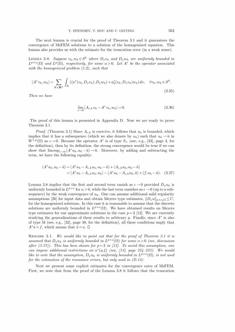
The next lemma is crucial for the proof of Theorem 3.1 and it guarantees theconvergence of MsFEM solutions to a solution of the homogenized equation. Thislemma also provides us with the estimate for the truncation error (in a weak sense).
Lemma 3.8. Suppose vh,wh∈Sh where Dxvh and Dxwh are uniformly bounded inLp+α(Ω) and Lp(Ω), respectively, for some α>0. Let A∗ be the operator associatedwith the homogenized problem (1.2), such that
〈A∗vh,wh〉=∑
K∈Kh
∫
K
((a∗(vh,Dxvh),Dxwh)+a∗0(vh,Dxvh)wh)dx, ∀vh,wh∈Sh.
(3.35)Then we have
limε→0
〈Aε,hvh−A∗vh,wh〉=0. (3.36)
The proof of this lemma is presented in Appendix D. Now we are ready to proveTheorem 3.1.
Proof. (Theorem 3.1) Since Aε,h is coercive, it follows that uh is bounded, whichimplies that it has a subsequence (which we also denote by uh) such that uh u inW 1,p(Ω) as ε→0. Because the operator A∗ is of type S+ (see, e.g., [33], page 3, forthe definition), then by its definition, the strong convergence would be true if we canshow that limsupε→0 〈A∗uh,uh− u〉→0. Moreover, by adding and subtracting theterm, we have the following equality:
〈A∗uh,uh− u〉= 〈A∗uh−Aε,huh,uh− u〉+〈Aε,huh,uh− u〉= 〈A∗uh−Aε,huh,uh〉−〈A∗uh−Aε,huh,u〉+(f,uh− u). (3.37)
Lemma 3.8 implies that the first and second term vanish as ε→0 provided Dxuh isuniformly bounded in Lp+α for α>0, while the last term vanishes as ε→0 (up to a sub-sequence) by the weak convergence of uh. One can assume additional mild regularityassumptions [26] for input data and obtain Meyers type estimates, ‖Dxu‖p+α,Ω≤C,for the homogenized solutions. In this case it is reasonable to assume that the discretesolutions are uniformly bounded in Lp+α(Ω). We have obtained results on Meyerstype estimates for our approximate solutions in the case p=2 [12]. We are currentlystudying the generalizations of these results to arbitrary p. Finally, since A∗ is alsoof type M (see, e.g., [32], page 38, for the definition), all these conditions imply thatA∗u=f , which means that u=u.
Remark 3.1. We would like to point out that for the proof of Theorem 3.1 it isassumed that Dxuh is uniformly bounded in Lp+α(Ω) for some α>0 (see, discussionafter (3.37)). This has been shown for p=2 in [12]. To avoid this assumption, onecan impose additional restrictions on a∗(η,ξ) (see, [13], page 254–255). We wouldlike to note that the assumption, Dxuh is uniformly bounded in Lp+α(Ω), is not usedfor the estimation of the resonance errors, but only used in (D.12).
Next we present some explicit estimates for the convergence rates of MsFEM.First, we note that from the proof of the Lemma 3.8 it follows that the truncation
564 MULTISCALE FINITE ELEMENT METHODS FOR NONLINEAR PROBLEMS
error of MsFEM (in a weak sense) is given by
〈Aε,huh−A∗uh,wh〉
= 〈f−A∗uh,wh〉≤ c( ε
h
) sp(p−s)
(|Ω|+‖uh‖p
p,Ω +‖Dxuh‖pp,Ω
) 1q ‖Dxwh‖p,Ω
+cε
h
(|Ω|+‖uh‖p
p,Ω +‖Dxuh‖pp,Ω
) 1q ‖Dxwh‖p,Ω +e(h)‖Dxwh‖p,Ω
= c
(( ε
h
) sp(p−s)
+ε
h
)(|Ω|+‖uh‖p
p,Ω +‖Dxuh‖pp,Ω
) 1q ‖Dxwh‖p,Ω +e(h)‖Dxwh‖p,Ω,
(3.38)
where e(h) is a generic sequence independent of small scale ε, such that e(h)→0 ash→0. In particular, the first, second, and third terms on the right side of (3.38) arethe estimates of
∑K∈Kh IK ,
∑K∈Kh IIK , and
∑K∈Kh IIIK , respectively (see (D.3)
and (D.4)). We note that the first term on the right side of (3.38) is the leading orderresonance error caused by the linear boundary conditions imposed on ∂K, the secondterm is due to mismatch between the mesh size and the small scale of the problem.These resonance errors are also present in the linear case [14]. If one uses the periodicsolution of the auxiliary problem for constructing the solutions of the local problems,then the resonance error can be removed. To obtain explicit convergence rates, wefirst derive upper bounds for 〈A∗uh−A∗Phu,uh−Phu〉, where Phu denotes a finiteelement projection of u onto Sh, i.e.,
〈A∗Phu,vh〉= 〈f,vh〉, ∀vh∈Sh,
and 〈A∗uh,vh〉 is defined by (3.35). Then using estimate (3.38), we have
〈A∗uh−A∗Phu,uh−Phu〉= 〈A∗uh−Aε,huh,uh−Phu〉+〈Aε,huh−A∗Phu,uh−Phu〉= 〈A∗uh−Aε,huh,uh−Phu〉+〈f−A∗Phu,uh−Phu〉= 〈A∗uh−Aε,huh,uh−Phu〉
≤ c
(( ε
h
) sp(p−s)
+ε
h
)(|Ω|+‖uh‖p
p,Ω +‖Dxuh‖pp,Ω
) 1q
‖Dx(uh−Phu)‖p,Ω +e(h)‖Dx(uh−Phu)‖p,Ω. (3.39)
The estimate (3.39) does not allow us to obtain an explicit convergence ratewithout some lower bound for the left side of the expression. In the proof of Theorem3.1, we only use the fact that A∗ is the operator of type S+, which guarantees that theconvergence of the left side of (3.39) to zero implies the convergence of the discretesolutions to a solution of the homogenized equation. Explicit convergence rates canbe obtained by assuming some kind of an inverse stability condition, ‖A∗u−A∗v‖≥c‖u−v‖. In particular, we may assume that A∗ is a monotone operator, i.e.,
〈A∗u−A∗v,u−v〉≥ c‖Dx(u−v)‖pp,Ω. (3.40)
A simple way to achieve monotonicity is to assume aε(x,η,ξ)=aε(x,ξ) anda0,ε(x,η,ξ)=0, though one can impose additional conditions on aε(x,η,ξ) and

Y. EFENDIEV, T. HOU AND V. GINTING 565
a0,ε(x,η,ξ), such that monotonicity condition (3.40) is satisfied. For our further cal-culations, we only assume (3.40). Then from (3.39) and (3.40), and using Younginequality, we have
‖Dx(uh−Phu)‖pp,Ω≤ c
( ε
h
) s(p−1)(p−s)
+c( ε
h
) pp−1
+e(h).
Next taking into account the convergence of standard finite element solutions of thehomogenized equation we write
‖DxPhu−Dxu‖p,Ω≤e1(h),
where e1(h)→0 (as h→0) is independent of ε. Consequently, using triangle inequalitywe have
‖Dx(uh−u)‖pp,Ω≤ c
( ε
h
) s(p−1)(p−s)
+c( ε
h
) pp−1
+e(h)+e1(h).
Proof. (Theorem 3.2). For monotone operators, aε(x,η,ξ)=aε(x,ξ) anda0,ε(x,η,ξ)=0, η∈R and ξ∈Rd, the estimates for e(h) and e1(h) can be easily de-rived. In particular, because of the absence of η in aε, e(h)=0 (see (D.3) and (D.4)),while e1(h)≤Ch
1p−1 (see for example [7]). Combining these estimates we have
‖Dx(uh−u)‖pp,Ω≤ c
( ε
h
) s(p−1)(p−s)
+c( ε
h
) pp−1
+chp
p−1 . (3.41)
From here one obtains (3.8).Remark 3.2. One can impose various conditions on the operators to obtain differentkinds of convergence rates. For example, under the additional assumptions (cf. [27])
|∂a∗(η,ξ)∂η
|+ |∂a∗(η,ξ)∂ξ
|≤C,∂a∗i (η,ξ)
∂ξjζiζj≥C|ζ|2, (3.42)
where ζ ∈Rd is an arbitrary vector, and p=2, following the analysis presented in [27],pages 51–52, the convergence rate in terms of Lp-norm of uh−Phu can be obtained,
‖Dx(uh−Phu)‖pp,Ω≤ c
( ε
h
) s(p−1)(p−s)
+c( ε
h
) pp−1
+e(h)+C‖uh−Phu‖pp,Ω,
where s∈ (0,1), p=2.
Remark 3.3. For the linear operators (p=2, s=1), we recover the convergence rateobtained in [20], Ch+C1
√ε/h.
Remark 3.4. We have shown that MsFEM for nonlinear problems has the same errorstructure as for the linear problems. In particular, our studies revealed two kinds ofresonance errors for nonlinear problems with the same nature as those that arise inlinear problems [14].
3.1. Approximation of the oscillations. In this section we present atheorem demonstrating the approximation of oscillatory solutions uε of (1.1).Theorem 3.9. Let uε be the solution of boundary value problem (1.1) and uh∈Sh anduε,h∈V h
ε with uε,h =EMsFEMuh be MsFEM solution (homogenized and fluctuatingcomponents, respectively) (2.3). Then limε→0 ‖Dxuε,h−Dxuε‖p,Ω =0.
566 MULTISCALE FINITE ELEMENT METHODS FOR NONLINEAR PROBLEMS
K
S
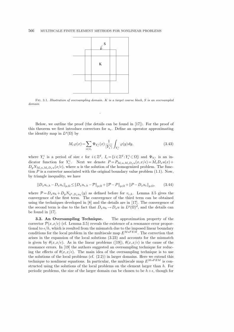
Fig. 3.1. Illustration of oversampling domain. K is a target coarse block, S is an oversampleddomain
.
Below, we outline the proof (the details can be found in [17]). For the proof ofthis theorem we first introduce correctors for uε. Define an operator approximatingthe identity map in Lp(Ω) by
Mεϕ(x)=∑
i∈Iε
ΨY iε(x)
1|Y i
ε |∫
Y iε
ϕ(y)dy, (3.43)
where Y iε is a period of size ε for i∈Zd, Iε =i∈Zd :Y i
ε ⊂Ω and ΨY iε
is an in-dicator function for Y i
ε . Next we denote P =PMεu,MεDxu(x,x/ε)=MεDxu(x)+DyNMεu,MεDxu(x/ε), where u is the solution of the homogenized problem. The func-tion P is a corrector associated with the original boundary value problem (1.1). Now,by triangle inequality, we have
‖Dxuε,h−Dxuε‖p,Ω≤‖Dxuε,h−P‖p,Ω +‖P−P‖p,Ω +‖P −Dxuε‖p,Ω, (3.44)
where P=Dxuh +DyNηh,Dxuh(y) as defined before for vε,h. Lemma 3.5 gives the
convergence of the first term. The convergence of the third term can be obtainedusing the techniques developed in [8] and the details are in [17]. The convergence ofthe second term is due to the fact that Dxuh→Dxu in Lp(Ω)d, and the details canbe found in [17].
3.2. An Oversampling Technique. The approximation property of thecorrector P(x,x/ε) (cf. Lemma 3.5) reveals the existence of a resonance error propor-tional to ε/h, which is resulted from the mismatch due to the imposed linear boundaryconditions for the local problem in the multiscale map EMsFEM . The correction thatarises in the expansion of the local solutions (3.23) and accounts for the mismatchis given by θ(x,x/ε). As in the linear problems ([19]), θ(x,x/ε) is the cause of theresonance errors. In [19] the authors suggested an oversampling technique for reduc-ing the effects of θ(x,x/ε). The main idea of the oversampling technique is to usethe solutions of the local problems (cf. (2.2)) in larger domains. Here we extend thistechnique to nonlinear equations. In particular, the multiscale map EMsFEM is con-structed using the solutions of the local problems on the element larger than h. Forperiodic problems, the size of the larger domain can be chosen to be h+ε, though for

Y. EFENDIEV, T. HOU AND V. GINTING 567
more general problems without scale separation the size of the larger domain can bechosen to be h+βh, where β is a constant. In our simulations for general anisotropicheterogeneities, we choose β =1. Furthermore, only the information from the targetelement is used in the multiscale formulation of the problem (see Figure 3.1).
In general, given vh∈Sh, where vh is defined in K, we want to find vε,h thatsatisfies
−div(aε(x,ηvh ,Dxvε,h))=0 in S (3.45)
such that vε,h(zi)=vh(zi), where zi are the nodal points of the target coarse elementK. Thus, in general, we need to find a solution of the local equation with given valuesat the nodal (interior) points. This problem can be solved for linear problems usinglinear combinations of the local solutions in larger domains S. Here we present anoversampling technique for special cases in which the gradient in the coefficient islinear, i.e., aε(x,η,ξ)=a(x/ε,η)ξ, given vh∈Sh, we define
vε,h =3∑
i=1
ciφiε, (3.46)
where φiε satisfies
−div(a(x/ε,ηvh)Dxφiε)=0 in S
φiε =φi
0 on ∂S.(3.47)
The constants ci, i=1,2,3 are determined by imposing the conditions
vε,h(zj)=vh(zj) j =1,2,3. (3.48)
We note that the piecewise constants in ηvh are taken as the average over the elementK. We would like to note that the convergence analysis of MsFEM with an over-sampling technique requires some modifications of the proof presented in this paperfor MsFEM without oversampling. In particular, the improved corrector results (seeLemma 3.5) are necessary to show the advantages of MsFEM with oversampling. Thisis a subject of our future research.
4. Numerical results and applications
4.1. Oversampling vs. non-oversampling. In this section we presentseveral ingredients pertaining to the implementation of the multiscale finite elementmethod. We will present numerical results for both MsFEM and the multiscale finitevolume element method (MsFVEM). We use an Inexact-Newton algorithm as aniterative technique to tackle the nonlinearity. For the numerical examples below, weuse aε(x,uε,Dxuε)=aε(x,uε)Dxuε. Let φi
0Ndof
i=1 be the standard piecewise linearbasis functions of Sh. Then the MsFEM solution may be written as
uh =Ndof∑
i=1
αiφi0 (4.1)
for some α=(α1,α2,··· ,αNdof)T , where αi depends on ε. Hence, we need to find α
such that
F (α)=0, (4.2)

568 MULTISCALE FINITE ELEMENT METHODS FOR NONLINEAR PROBLEMS
Table 4.1. Relative MsFEM Errors without Oversampling
N L2-norm H1-norm L∞-normError Rate Error Rate Error Rate
32 0.029 0.115 0.0364 0.053 -0.85 0.156 -0.44 0.0534 -0.94
128 0.10 -0.94 0.234 -0.59 0.10 -0.94
where F :RNdof →RNdof is a nonlinear operator such that
Fi(α)=∑
K∈Kh
∫
K
(aε(x,ηuh)Dxuε,h),Dxφi0)dx−
∫
Ω
f φi0dx. (4.3)
We note that in (4.3) α is implicitly buried in ηuh and uε,h. An inexact-Newtonalgorithm is a variation of Newton’s iteration for a nonlinear system of equations,where the Jacobian system is only approximately solved. To be specific, given aninitial iterate α0, for k =0,1,2,··· until convergence do the following:
• Solve F ′(αk)δk =−F (αk) by some iterative technique until ‖F (αk)+F ′(αk)δk‖≤ βk ‖F (αk)‖.
• Update αk+1 =αk +δk.In this algorithm F ′(αk) is the Jacobian matrix evaluated at iteration k. We notethat when βk =0 then we have recovered the classical Newton iteration. Here we haveused
βk =0.001( ‖F (αk)‖‖F (αk−1)‖
)2
, (4.4)
with β0 =0.001. Choosing βk this way, we avoid over-solving the Jacobian systemwhen αk is still considerably far from the exact solution.
Next we present the entries of the Jacobian matrix. For this purpose, weuse the following notations. Let Kh
i =K ∈Kh :zi is a vertex of K, Ii =j :zj is a vertex of K ∈Kh
i , and Khij =K ∈Kh
i :K shares zizj. We note that we maywrite Fi(α) as follows:
Fi(α)=∑
K∈Khi
(∫
K
(aε(x,ηuh)Dxuε,h,Dxφi0)dx−
∫
K
f φi0dx
), (4.5)
with
−div(aε(x,ηuh)Dxuε,h)=0 in K and uε,h =∑
zm∈ZK
αmφm0 on ∂K, (4.6)
where ZK is all the vertices of element K. It is apparent that Fi(α) is not fullydependent on all α1,α2,··· ,αd. Consequently, ∂Fi(α)
∂αj=0 for j /∈ Ii. To this end, we
denote ψjε = ∂uε,h
∂αj. By applying the chain rule of differentiation to (4.6) we have the
following local problem for ψjε :
−div(aε(x,ηuh)Dxψjε )=
13
div(∂aε(x,ηuh)
∂uDxuε,h) in K and ψj
ε =φjε on ∂K.
(4.7)

Y. EFENDIEV, T. HOU AND V. GINTING 569
Table 4.2. Relative MsFVEM Errors without Oversampling
.9 N L2-norm H1-norm L∞-normError Rate Error Rate Error Rate
32 0.03 0.13 0.0464 0.05 -0.65 0.19 -0.60 0.05 -0.24
128 0.058 -0.19 0.25 -0.35 0.057 -0.19
Table 4.3. Relative MsFEM Errors with Oversampling
N L2-norm H1-norm L∞-normError Rate Error Rate Error Rate
32 0.0016 0.036 0.002964 0.0012 0.38 0.019 0.93 0.0016 0.92
128 0.0024 -0.96 0.0087 1.14 0.0026 -0.71
The fraction 1/3 comes from taking the derivative in the chain rule of differenti-ation. In the formulation of the local problem, we have replaced the nonlinearityin the coefficient by ηvh , where for each triangle K ηvh =1/3
∑3i=1αK
i , which gives∂ηvh/∂αi =1/3. Moreover, for a rectangular element the fraction 1/3 should be re-placed by 1/4.
Thus, provided that vε,h has been computed, then we may compute ψjε using
(4.7). Using the above descriptions we have the expressions for the entries of theJacobian matrix:
∂Fi
∂αi=
∑
K∈Khi
(13
∫
K
(∂aε(x,ηuh)
∂uDxuε,h,Dxφi
0)dx+∫
K
(aε(x,ηuh)Dxψi,Dxφi0)dx,
)
(4.8)
∂Fi
∂αj=
∑
K∈Khij
(13
∫
K
(∂aε(x,ηuh)
∂uDxuε,h,Dxφi
ε)dx+∫
K
(aε(x,ηuh)Dxψjε ,Dxφi
0)dx,
)
(4.9)for j 6= i, j∈ Ii.
The implementation of the oversampling technique is similar to the procedurepresented above, except the local problems in larger domains are used. From (3.46),(3.47), and (3.48) we obtain vε,h that satisfies the homogeneous local problem. As inthe non-oversampling case, we denote ψj
ε = ∂vε,h
∂αj, such that after applying the chain
rule of differentiation to the local problem we have:
−div(aε(x,ηuh)Dxψjε )=
13
div(∂aε(x,ηuh)
∂uDxvε,h) in S and ψj
ε =φj0 on ∂S,
(4.10)where ηuh is computed over the corresponding element K and φj
0 is understood asthe nodal basis functions on oversampled domain S. Then all the rest of the inexact-Newton algorithms are the same as in the non-oversampling case. Specifically, we alsouse (4.8) and (4.9) to construct the Jacobian matrix of the system. We note that wewill only use ψj
ε from (4.10) pertaining to the element K.

570 MULTISCALE FINITE ELEMENT METHODS FOR NONLINEAR PROBLEMS
Table 4.4. Relative MsFVEM Errors with Oversampling
N L2-norm H1-norm L∞-normError Rate Error Rate Error Rate
32 0.002 0.038 0.00564 0.003 -0.43 0.021 0.87 0.003 0.72
128 0.001 1.10 0.009 1.09 0.001 1.08
Table 4.5. Relative MsFEM Errors for random heterogeneities, spherical variogram, lx =0.20,lz =0.02, σ =1.0
N L2-norm H1-norm L∞-norm hor. fluxError Rate Error Rate Error Rate Error Rate
32 0.0006 0.0505 0.0025 0.02564 0.0002 1.58 0.029 0.8 0.001 1.32 0.017 0.57
128 0.0001 1 0.016 0.85 0.0005 1 0.011 0.62
From the derivation (both for oversampling and non-oversampling) it is obviousthat the Jacobian matrix is not symmetric but sparse. Computation of this Jacobianmatrix is similar to computing the stiffness matrix resulting from a standard finiteelement, where each entry is formed by accumulation of element by element contri-bution. Once we have the matrix stored in memory, then its action to a vector isstraightforward. Because it is a sparse matrix, devoting some amount of memoryfor entries storage is inexpensive. The resulting linear system is solved using thepreconditioned bi-conjugate gradient stabilized method.
We want to solve the following problem:
−div(a(x/ε,uε)Dxuε)=−1 in Ω⊂R2,
uε =0 on ∂Ω,(4.11)
where Ω=[0,1]× [0,1], a(x/ε,uε)=k(x/ε)/(1+uε)l(x/ε), with
k(x/ε)=2+1.8sin(2πx1/ε)2+1.8cos(2πx2/ε)
+2+sin(2πx2/ε)
2+1.8cos(2πx1/ε)(4.12)
and l(x/ε) is generated from k(x/ε) such that the average of l(x/ε) over Ω is 2. Here weuse ε=0.01. Because the exact solution for this problem is not available, we use a wellresolved numerical solution using the standard finite element method as a referencesolution. The resulting nonlinear system is solved using an inexact-Newton algorithm.The reference solution is solved on 512×512 mesh. Tables 4.1 and 4.3 present therelative errors of the solution with and without oversampling, respectively. In tables4.2 and 4.4, the relative errors for the multiscale finite volume element method arepresented. The relative errors are computed as the corresponding error divided bythe norm of the solution. In each table, the second, third, and fourth columns list therelative error in L2, H1, and L∞ norm, respectively. As we can see from these twotables, the oversampling significantly improves the accuracy of the multiscale method.
For our next example, we consider the problem with non-periodic coefficients,where aε(x,η)=kε(x)/(1+η)αε(x). kε(x)=exp(βε(x)) is chosen such that βε(x) is a
Y. EFENDIEV, T. HOU AND V. GINTING 571
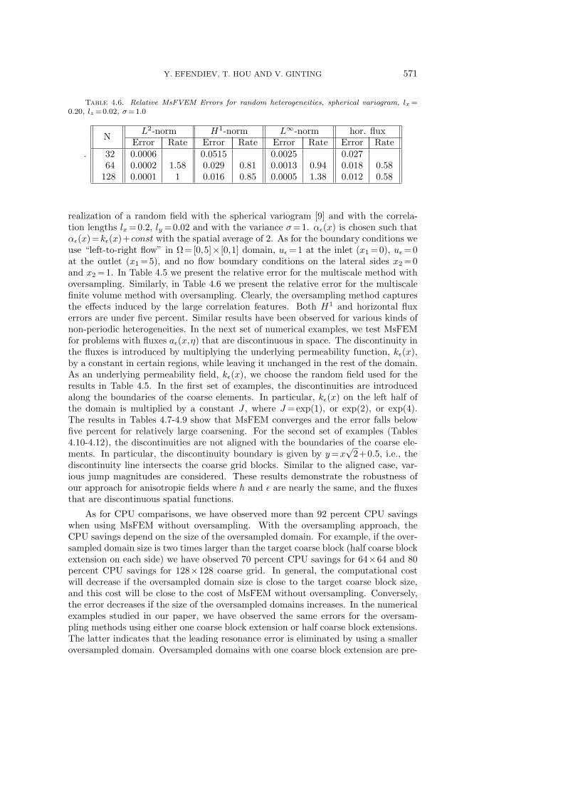
Table 4.6. Relative MsFVEM Errors for random heterogeneities, spherical variogram, lx =0.20, lz =0.02, σ =1.0
.
N L2-norm H1-norm L∞-norm hor. fluxError Rate Error Rate Error Rate Error Rate
32 0.0006 0.0515 0.0025 0.02764 0.0002 1.58 0.029 0.81 0.0013 0.94 0.018 0.58
128 0.0001 1 0.016 0.85 0.0005 1.38 0.012 0.58
realization of a random field with the spherical variogram [9] and with the correla-tion lengths lx =0.2, ly =0.02 and with the variance σ =1. αε(x) is chosen such thatαε(x)=kε(x)+const with the spatial average of 2. As for the boundary conditions weuse “left-to-right flow” in Ω=[0,5]× [0,1] domain, uε =1 at the inlet (x1 =0), uε =0at the outlet (x1 =5), and no flow boundary conditions on the lateral sides x2 =0and x2 =1. In Table 4.5 we present the relative error for the multiscale method withoversampling. Similarly, in Table 4.6 we present the relative error for the multiscalefinite volume method with oversampling. Clearly, the oversampling method capturesthe effects induced by the large correlation features. Both H1 and horizontal fluxerrors are under five percent. Similar results have been observed for various kinds ofnon-periodic heterogeneities. In the next set of numerical examples, we test MsFEMfor problems with fluxes aε(x,η) that are discontinuous in space. The discontinuity inthe fluxes is introduced by multiplying the underlying permeability function, kε(x),by a constant in certain regions, while leaving it unchanged in the rest of the domain.As an underlying permeability field, kε(x), we choose the random field used for theresults in Table 4.5. In the first set of examples, the discontinuities are introducedalong the boundaries of the coarse elements. In particular, kε(x) on the left half ofthe domain is multiplied by a constant J , where J =exp(1), or exp(2), or exp(4).The results in Tables 4.7-4.9 show that MsFEM converges and the error falls belowfive percent for relatively large coarsening. For the second set of examples (Tables4.10-4.12), the discontinuities are not aligned with the boundaries of the coarse ele-ments. In particular, the discontinuity boundary is given by y =x
√2+0.5, i.e., the
discontinuity line intersects the coarse grid blocks. Similar to the aligned case, var-ious jump magnitudes are considered. These results demonstrate the robustness ofour approach for anisotropic fields where h and ε are nearly the same, and the fluxesthat are discontinuous spatial functions.
As for CPU comparisons, we have observed more than 92 percent CPU savingswhen using MsFEM without oversampling. With the oversampling approach, theCPU savings depend on the size of the oversampled domain. For example, if the over-sampled domain size is two times larger than the target coarse block (half coarse blockextension on each side) we have observed 70 percent CPU savings for 64×64 and 80percent CPU savings for 128×128 coarse grid. In general, the computational costwill decrease if the oversampled domain size is close to the target coarse block size,and this cost will be close to the cost of MsFEM without oversampling. Conversely,the error decreases if the size of the oversampled domains increases. In the numericalexamples studied in our paper, we have observed the same errors for the oversam-pling methods using either one coarse block extension or half coarse block extensions.The latter indicates that the leading resonance error is eliminated by using a smalleroversampled domain. Oversampled domains with one coarse block extension are pre-

572 MULTISCALE FINITE ELEMENT METHODS FOR NONLINEAR PROBLEMS
Table 4.7. Relative MsFEM Errors for random heterogeneities, spherical variogram, lx =0.20,lz =0.02, σ =1.0, aligned discontinuity, jump = exp(1)
.
N L2-norm H1-norm L∞-norm hor. fluxError Rate Error Rate Error Rate Error Rate
32 0.0006 0.0641 0.0020 0.03964 0.0002 1.58 0.0382 0.75 0.0010 1.00 0.027 0.53
128 0.0001 1.00 0.0210 0.86 0.0005 1.00 0.018 0.59
Table 4.8. Relative MsFEM Errors for random heterogeneities, spherical variogram, lx =0.20,lz =0.02, σ =1.0, aligned discontinuity, jump = exp(2)
N L2-norm H1-norm L∞-norm hor. fluxError Rate Error Rate Error Rate Error Rate
32 0.0008 0.0817 0.0040 0.06164 0.0004 1.00 0.0493 0.73 0.0023 0.80 0.041 0.57
128 0.0002 1.00 0.0256 0.95 0.0011 1.06 0.025 0.71
viously used in simulations of flow through heterogeneous porous media [36]. As itis indicated in [19], one can use large oversampled domains for simultaneous compu-tations of the several local solutions. Moreover, parallel computations will improvethe speed of the method because MsFEM is well suited for parallel computation [19].For the problems where aε(x,η,ξ)=aε(x)b(η)ξ (see section 2.2 and the next sectionfor applications) our multiscale computations are very fast because the base functionsare built in the beginning of the computations. In this case, we have observed morethan 95 percent CPU savings.
4.2. Applications of MsFEM to Richards’ equation. In this sectionwe consider the applications of MsFEM to Richards’ equation, which describes theinfiltration of water flow into a porous media whose pore space is filled with air andsome water. The equation describing Richards’ equation under some assumptions isgiven by
Dtθ(u)−div(K(x,u)Dx(u+x3))=0 inΩ, (4.13)
where θ(u) is volumetric water content and u is the pressure. The followings areassumed ([30]) for (4.13): (1) the porous medium and water are incompressible; (2)the temporal variation of the water saturation is significantly larger than the temporalvariation of the water pressure; (3) air phase is infinitely mobile so that the air pressureremains constant, in this case it is atmospheric pressure which equals zero; (4) neglectthe source/sink terms.
Constitutive relations between θ and u and between K and u are developed ap-propriately, which consequently gives nonlinearity behavior in (4.13). The relationbetween the water content and pressure is referred to as the moisture retention func-tion. The equation written in (4.13) is called the coupled-form of Richards’ Equation.In other literature this equation is also called the mixed form of Richards’ Equation,due to the fact that there are two variables involved in it, namely, the water content θand the pressure head u. Taking advantage of the differentiability of the soil retention

Y. EFENDIEV, T. HOU AND V. GINTING 573
Table 4.9. Relative MsFEM Errors for random heterogeneities, spherical variogram, lx =0.20,lz =0.02, σ =1.0, aligned discontinuity, jump = exp(4)
N L2-norm H1-norm L∞-norm hor. fluxError Rate Error Rate Error Rate Error Rate
32 0.0011 0.1010 0.0068 0.19564 0.0006 0.87 0.0638 0.66 0.0045 0.59 0.109 0.84
128 0.0003 1.00 0.0349 0.87 0.0024 0.91 0.063 0.79
Table 4.10. Relative MsFEM Errors for random heterogeneities, spherical variogram, lx =0.20,lz =0.02, σ =1.0, nonaligned discontinuity, jump = exp(1)
N L2-norm H1-norm L∞-norm hor. fluxError Rate Error Rate Error Rate Error Rate
32 0.0006 0.0623 0.0023 0.03564 0.0002 1.58 0.0366 0.77 0.0014 0.72 0.024 0.54
128 0.0001 1.00 0.0203 0.85 0.0006 1.22 0.016 0.59
function, one may rewrite (4.13) as follows:
C(u)Dtu−div(K(x,u)Dx(u+x3))=0 inΩ, (4.14)
where C(u)=dθ/du is the specific moisture capacity. This version is referred to asthe head-form (h-form) of Richards’ Equation. Another formulation of the Richards’Equation is based on the water content θ,
Dtθ−div(D(x,θ)Dxθ)− ∂K
∂x3=0 inΩ, (4.15)
where D(θ)=K(θ)/(dθ/du) defines the diffusivity. This form is called the θ-form ofRichards’ Equation.
The sources of nonlinearity of Richards’ Equation comes from the moisture re-tention and relative hydraulic conductivity functions, θ(u) and K(x,u), respectively.Reliable approximation of these relations are in general tedious to develop and thusalso challenging. Field measurements or laboratory experiments to gather the param-eters are relatively expensive, and furthermore, even if one can come up with suchrelations from these works, they will be somehow limited to the particular cases underconsideration.
Perhaps the most widely used empirical constitutive relations for the moisturecontent and hydraulic conductivity is due to the work of van Genuchten [34]. Heproposed a method of determining the functional relation of relative hydraulic con-ductivity to the pressure head by using the field observation knowledge of the mois-ture retention. In turn, the procedure would require curve-fitting to the proposedmoisture retention function with the experimental/observational data to establishcertain parameters inherent to the resulting hydraulic conductivity model. Thereare several widely known formulations of the constitutive relations: Haverkampmodel - θ(u)= α(θs−θr)
α+|u|β +θr, K(x,u)=Ks(x) AA+|u|γ ; van Genuchten model [34]
- θ(u)= α(θs−θr)[1+(α|u|)n]m +θr, K(x,u)=Ks(x)1−(α|u|)n−1[1+(α|u|)n]−m2
[1+(α|u|)n]m/2 ; Exponential
model [35] - θ(u)=θseβu, K(x,u)=Ks(x)eαu.

574 MULTISCALE FINITE ELEMENT METHODS FOR NONLINEAR PROBLEMS
Table 4.11. Relative MsFEM Errors for random heterogeneities, spherical variogram, lx =0.20,lz =0.02, σ =1.0, nonaligned discontinuity, jump = exp(2)
.
N L2-norm H1-norm L∞-norm hor. fluxError Rate Error Rate Error Rate Error Rate
32 0.0010 0.0785 0.0088 0.05264 0.0003 1.74 0.0440 0.84 0.0052 0.76 0.031 0.75
128 0.0001 1.59 0.0239 0.88 0.0022 1.24 0.017 0.87
Table 4.12. Relative MsFEM Errors for random heterogeneities, spherical variogram, lx =0.20,lz =0.02, σ =1.0, nonaligned discontinuity, jump = exp(4)
.
N L2-norm H1-norm L∞-norm hor. fluxError Rate Error Rate Error Rate Error Rate
32 0.0067 0.1775 0.1000 0.16464 0.0016 2.07 0.0758 1.23 0.0288 1.80 0.077 1.09
128 0.0009 0.83 0.0687 0.14 0.0423 -0.55 0.039 0.98
The variable Ks in the above models is also known as the saturated hydraulicconductivity. It has been observed that the hydraulic conductivity has a broad rangeof values, which together with the functional forms presented above, confirm thenonlinear behavior of the process. Furthermore, the water content and hydraulicconductivity approach zero as the pressure head goes to very large negative values.In other words, the Richards’ Equation has a tendency to degenerate in a very drycondition, i.e., conditions with the large negative pressure. Because we are interestedin mass conservative schemes, finite volume formulation (2.5) of the global probleminstead of finite element formulation will be used. For (4.13), it is to find uh∈Sh suchthat
∫
Vz
(θ(ηuh)−θn−1)dx−∆t
∫
∂Vz
K(x,ηuh)Dxuε,h ·ndl=0 ∀z∈Z0h, (4.16)
where θn−1 is the value of θ(ηuh) evaluated at time step n−1, and uε,h∈V hε is a
function that satisfies the boundary value problem:
−div(K(x,ηuh)Dxuε,h)=0 in K ∈Sh,
uε,h =uh on ∂K. (4.17)
Here Vz is the control volume surrounding the vertex z∈Z0h and Z0
h is the collectionof all vertices that do not belong to the Dirichlet boundary.
MsFEM (or MsFVEM) offers great advantage when the nonlinearity and hetero-geneity of K(x,p) is separable, i.e.,
K(x,u)=ks(x)kr(u). (4.18)
In this case, as we discussed earlier, the local problems become linear and the corre-sponding V h
ε is a linear space, i.e., we may construct a set of basis functions ψzz∈Z0h
such that they satisfy
−div(ks(x)Dxψz)=0 in K ∈Sh,
ψz =φz on ∂K, (4.19)

Y. EFENDIEV, T. HOU AND V. GINTING 575
ΓL
ΓR
ΓB
ΓT
L x
L z
Fig. 4.1. Rectangular porous medium
where φz is a piecewise linear function. We note that if uh has a discontinuity or asharp front region, then the multiscale basis functions need to be updated only in thatregion. The latter is similar to the use of MsFEM in two-phase flow applications. Forthis case the base functions are only updated along the front. Now, we may formulatethe finite dimensional problem. We want to seek uε,h∈V h
ε with uε,h =∑
z∈Z0hpzψz
such that∫
Vz
(θ(ηuh)−θn−1)dx−∆t
∫
∂Vz
ks(x)kr(ηuh)Dxuε,h ·ndl=0, (4.20)
for every control volume Vz⊂Ω. To this equation we can directly apply the lineariza-tion procedure described in [17]. Let us here denote
rm =umε,h−um−1
ε,h , m=1,2,3,·, (4.21)
where umε,h is the iterate of uε,h at the iteration level m. Thus, we want to find rm =∑
z∈Z0hrmz ψz such that for m=1,2,3,··· ‖rm‖≤ δ with δ being some predetermined
error tolerance∫
Vz
C(ηuh,m−1)rmdx−∆t
∫
∂Vz
ks(x)kr(ηuh,m−1)Dxrm ·ndl=Rh,m−1, (4.22)
with
Rh,m−1 =−∫
Vz
(θ(ηuh,m−1)−θn−1)dx+∆t
∫
∂Vz
ks(x)kr(ηuh,m−1)Dxum−1ε,h ·ndl.
(4.23)The superscript m at each of the functions means that the corresponding functionsare evaluated at an iteration level m.
We present several numerical experiments that demonstrate the ability of thecoarse models presented in the previous subsections. The coarse models are comparedwith the fine model solved on a fine mesh. We have employed a finite volume differenceto solve the fine-scale equations. This solution serves as a reference for the proposedcoarse models. The problems that we consider are typical water infiltration into aninitially dry soil. The porous medium that we consider is a rectangle of size Lx×Lz

576 MULTISCALE FINITE ELEMENT METHODS FOR NONLINEAR PROBLEMS
Fig. 4.2. Haverkamp model with isotropic heterogeneity. Comparison of water pressure betweenthe fine model (left) and the coarse model (right).
(see Figure 4.1). The fine model uses 256×256 rectangular elements, while the coarsemodel uses 32×32 rectangular elements.
A realization of the permeability field is generated using geostatistical packageGSLIB ([9]). We have used a spherical variogram with prescribed correlation lengths(lx, lz) and the variance (σ) for this purpose. All examples use σ =1.5.
The first problem is a soil infiltration, which was first analyzed by Haverkamp(cf. [6]). The porous medium dimension is Lx =40 and Lz =40. The boundaryconditions are as follows: ΓL and ΓR are impermeable, while Dirichlet conditionsare imposed on ΓB and ΓT , namely uT =−21.7 in ΓT , and uB =−61.5 in ΓB . Theinitial pressure is u0 =−61.5. The constitutive relations use the Haverkamp model.The related parameters are as follows: α=1.611×10⁶, θs =0.287, θr =0.075, β =3.96,A=1.175×10⁶, and γ =4.74. For this problem we assume that the nonlinearity andheterogeneity are separable, where the latter comes from Ks(x) with Ks =0.00944.We assume that appropriate units for these parameters hold. There are two casesconsidered for this problem, namely, the isotropic heterogeneity with lx = lz =0.1,and the anisotropic heterogeneity with lx =0.01 and lz =0.20. For the backwardEuler scheme, we use ∆t=10. Note that the large value of ∆t is due to the smallnessof Ks (average magnitude of the diffusion). The comparison is shown in Figures 4.2and 4.3, where the solutions are plotted at t=360.
The second problem is a soil infiltration through a porous medium whose dimen-sion is Lx =1 and Lz =1. The boundary conditions are as follows: ΓL and ΓR areimpermeable. Dirichlet conditions are imposed on ΓB with uB =−10. The bound-ary ΓT is divided into three parts. On the middle part, a zero Dirichlet conditionis imposed, and the rest are impermeable. The constitutive relations use the Expo-nential model with the following related parameters: β =0.01, θs =1, Ks=1, andα=0.01. The heterogeneity comes from Ks(x) and α(x). Clearly, for this problemthe nonlinearity and heterogeneity are not separable. Again, isotropic and anisotropicheterogeneities are considered with lx = lz =0.1 and lx =0.20, lz =0.01, respectively.For the backward Euler scheme, we use ∆t=2. The comparison is shown in Figures4.4 and 4.5, where the solutions are plotted at t=10.
We note that the problems that we have considered are vertical infiltration onthe porous medium. Hence, it is also useful to compare the cross-sectional vertical

Y. EFENDIEV, T. HOU AND V. GINTING 577
Fig. 4.3. Haverkamp model with anisotropic heterogeneity. Comparison of water pressurebetween the fine model (left) and the coarse model (right).
Fig. 4.4. Exponential model with isotropic heterogeneity. Comparison of water pressure betweenthe fine model (left) and the coarse model (right).
Fig. 4.5. Exponential model with anisotropic heterogeneity. Comparison of water pressurebetween the fine model (left) and the coarse model (right).

578 MULTISCALE FINITE ELEMENT METHODS FOR NONLINEAR PROBLEMS
velocity that will be plotted against the depth z. Here, the cross-sectional verticalvelocity is obtained by taking an average over the horizontal direction (x-axis).
0 10 20 30 40−2.5
−2
−1.5
−1
−0.5
0 x 10−3
z
Ve
rtic
al V
elo
city
Fine ModelCoarse Model
0 10 20 30 40−4
−3.5
−3
−2.5
−2
−1.5
−1
−0.5
0 x 10−3
z
Ve
rtic
al V
elo
city
Fine ModelCoarse Model
Fig. 4.6. Comparison of vertical velocity on the coarse grid for Haverkamp model: isotropicheterogeneity (left) and anisotropic heterogeneity (right).
0 0.2 0.4 0.6 0.8 1−18
−16
−14
−12
−10
−8
−6
−4
z
Ve
rtic
al V
elo
city
Fine ModelCoarse Model
0 0.2 0.4 0.6 0.8 1−10
−9
−8
−7
−6
−5
−4
−3
z
Ve
rtic
al V
elo
city
Fine ModelCoarse Model
Fig. 4.7. Comparison of vertical velocity on the coarse grid for Exponential model: isotropicheterogeneity (left) and anisotropic heterogeneity (right). The average is taken over the second thirdof the domain.
Figure 4.6 shows a comparison of the cross-sectional vertical velocity for theHaverkamp model. The average is taken over all the horizontal span because theboundary condition on ΓT (and also on ΓB) is all Dirichlet condition. Both plotsin this figure show a close agreement between the fine and coarse models. For theExponential model, as we have described above, there are three different segments forthe boundary condition on ΓT , i.e., a Neumann condition on the first and third part,and a Dirichlet condition on the second/middle part of ΓT . Thus, we will comparethe cross-sectional vertical velocity in each of these segments separately. Figure 4.7

Y. EFENDIEV, T. HOU AND V. GINTING 579
shows the comparison for one of these segments. The agreement between the coarsegrid and fine grid calculations is excellent.
5. Extension of MsFEM and concluding remarks
5.1. On the convergence of MsFEM. In this paper we have discussedthe convergence of MsFEM in the limit ε/h→0 for the periodic problems. Thisresult, we believe, also holds for nonlinear elliptic problems with random homogeneouscoefficients, where we assume aε(x,η,ξ)=a(T (x/ε)ω,η,ξ), where a(ω,η,ξ) is a randomhomogeneous field. The analysis of the case with random heterogeneities is differentfrom the periodic case and it is currently under investigation. For more general caseswithout any assumptions on the nature of heterogeneities, one can show (see [13])
limh→0
limε→0
‖uh−u‖W 1,p0 (Ω) =0, (5.1)
(up to a subsequence) where u can be a solution of (1.2) and uh is a MsFEM solutiongiven by (2.3). The proof of this fact uses only G-convergence results and holds up toa subsequence of ε. As we mentioned before, this result can not be improved becausethere could be infinitely many scales (α(ε)) such that α(ε)→0 as ε→0.
5.2. MsFEM for nonlinear parabolic equations. Consider uε∈W0
Dtuε−div(aε(x,t,uε,Dxuε))+a0,ε(x,t,uε,Dxuε)=f,
where W0 =u∈W,u(x,t=0)=0, and
V0 =Lp(0,T,W 1,p0 (Ω)),
V =Lp(0,T,W 1,p(Ω)),W =u∈V0,Dtu∈Lq(0,T,W−1,q(Ω)),W =u∈V ,Dtu∈Lq(0,T,W−1,q(Ω)). (5.2)
Assume 0= t0 <t1 < ···<tM =T , where max(ti+1− ti)=ht and denote h=max(hx,ht). The multiscale mapping for nonlinear parabolic equations, EMsFEM :Sh→V h
ε , is constructed in the following way. For each vh∈Sh, vε,h(x,t) is the solutionof
Dtvε,h−div(aε(x,t,ηvh ,Dxvε,h))=0 in K× [tn,tn+1], (5.3)
vε,h =vh on ∂K and vε,h(t= tn)=vh. Note that EMsFEM is a one-to-one map definedon Ω× [tn,tn+1]. MsFEM formulation of the problem is the following. Find uh(t)∈Sh
(and uε,h∈V hε ) such that
∫ tn+1
tn
∫
Ω
Dtuhvhdxdt+〈Aε,huh,vh〉=∫ tn+1
tn
∫
Ω
fvhdxdt, (5.4)
where
〈Aε,huh,vh〉=∫ tn+1
tn
∫
Ω
((aε(x,t,ηuh ,Dxuε,h),Dxvh)+a0,ε(x,t,ηuh ,Dxuε,h)vh)dxdt.
One can write (5.4) in the following way∫
Ω
(uh(tn+1)−uh(tn))vhdx+〈Aε,huh,vh〉=∫ tn+1
tn
∫
Ω
fvhdxdt.

580 MULTISCALE FINITE ELEMENT METHODS FOR NONLINEAR PROBLEMS
Furthermore, taking the present value of uh, i.e., uh(x,tn+1), in 〈Aε,huh,vh〉 we obtainthe implicit MsFEM scheme and taking the value of uh at t= tn we obtain the explicitMsFEM scheme. For the special periodic case, one can use the solution in the periodto construct EMsFEM as we did in the elliptic case. Finally, we would like to notethat one can develop oversampling techniques for parabolic problems, by extendingboth temporal and spatial domains of the local problems, and this is a subject of ourfuture research.
Next, we consider some concrete examples.Example 1. Linear Case.In the linear case, the multiscale map EMsFEM is linear, and consequently, V h
ε is alinear space. A basis of V h
ε can be found by mapping a basis of Sh, i.e., V hε =span(φi
ε),where φi
ε satisfy
Dtφiε−div(aε(x,t)Dxφi
ε)=0 in K× [tn,tn+1], (5.5)
φiε(t= tn)=φi
0 on ∂K and φiε =φi
0, where Sh =span(φi0). The development of the
oversampling techniques for both space and time is currently under investigation.Example 2. Spatial caseIf we assume aε(x,t,η,ξ) is independent of time, then the following local problems
can be solved for the construction of EMsFEM (instead of (5.3))
−div(aε(x,ηvh ,Dxvε,h))=0 in K× [tn,tn+1], (5.6)
where vε,h =vh on ∂K and vε,h(t= tn)=vh. This simplification of the local problemcan be understood based on the homogenization of parabolic equations. In particular,the solution of (5.3) can be approximated with the solution of (5.6) in the case ofspatial heterogeneities.
5.3. Further generalizations of MsFEM and concluding remarks.Next, we present the framework of MsFEM for general equations. Consider
Lεuε =f, (5.7)
where ε is a small scale and Lε :X→Y is an operator. Moreover, we assume that Lε
G-converges to L∗ (up to a sub-sequence), where u is a solution of
L∗u=f, (5.8)
(we refer to [28], page 14 for the definition of G-convergence for operators). The ob-jective of MsFEM is to approximate u in Sh. Denote Sh a family of finite dimensionalspace such that it possesses an approximation property (see [37, 29]) as before. Here his a scale of computation and hÀ ε. For (5.7) multiscale mapping, EMsFEM :Sh→V h
ε
, will be defined as follows. For each element vh∈Sh, vε,h =EMsFEMvh is defined as
Lmapε vε,h =0 in K, (5.9)
where Lmapε can be, in general, different from Lε and allows us to capture the effects of
the small scales. Moreover, the domains different from the target coarse block K canbe used in the computations of the local solutions. To solve (5.9) one needs to imposeboundary and initial conditions. This issue needs to be resolved on a case by casebasis, and the main idea is to interpolate vh onto the underlying fine grid. Further,

Y. EFENDIEV, T. HOU AND V. GINTING 581
we seek a solution of (5.7) in V hε as follows. Find uh∈Sh (consequently uε,h∈V h
ε )such that
〈Lglobalε uε,h,vh〉= 〈f,vh〉, ∀vh∈Sh, (5.10)
where 〈u,v〉 denotes the duality between X and Y , and Lglobalε can be, in gen-
eral, different from Lε. For example, for nonlinear elliptic equations we have Lεu=−div(aε(x,u,Dxu))+a0,ε(x,u,Dxu), Lmap
ε u=div(aε(x,ηu,Dxu)) in K, and Lglobalε =
div(aε(x,ηu,Dxu))+a0,ε(x,ηu,Dxu) in K. The convergence of MsFEM is to showthat uh→u and uε,h→uε, where uε,h =EMsFEMuh in appropriate space. The cor-rect choices of Lmap
ε and Lglobalε are the essential part of MsFEM and guarantees the
convergence of the method.In conclusion, we have presented a natural extension of MsFEM to nonlinear
problems. This is accomplished by considering a multiscale map instead of the basefunctions that are considered in linear MsFEM [19]. Our approaches share some com-mon elements with recently introduced HMM [10], where macroscopic and microscopicsolvers are also needed. In general, the finding of “correct” macroscopic and micro-scopic solvers is the main difficulty of the multiscale methods. Our approaches followMsFEM and, consequently, finite element methods constitute its main ingredient.The resonance errors, that arise in linear problems also arise in nonlinear problems.Note that the resonance errors are the common feature of multiscale methods unlessperiodic problems are considered and the solutions of the local problems in an exactperiod are used. To reduce the resonance errors we use an oversampling techniqueand show that the error can be greatly reduced by sampling from the larger domains.The multiscale map for MsFEM uses the solutions of the local problems in the targetcoarse block. This way one can sample the heterogeneities of the coarse block. Ifthere is a scale separation and, in addition, some kind of periodicity, one can use thesolutions of the smaller size problems to approximate the multiscale map. Note thata potential disadvantage of periodicity assumption is that the periodicity can act todisrupt large-scale connectivity features of the flow. For the examples similar to thenon-periodic ones considered in this paper, with the use of the smaller size problemsfor approximating the solutions of the local problems, we have found very large errors(of order 50 percent).
Appendix A. The proof of Lemma 3.3.Let vε,h =vε,h−vh, where vε,h =EMsFEMvh. It follows that vε,h∈W 1,p
0 (K) sat-isfies the following problem:
−div(aε(x,ηvh ,Dxvε,h +Dxvh))=0 in K. (A.1)
Using (A.1), applying Green’s Theorem we have the following estimate:
〈Aε,hvh,vh〉=
∑
K∈Kh
∫
K
(aε(x,ηvh ,Dxvh +Dxvε,h),Dxvh +Dxvε,h)dx
+∑
K∈Kh
∫
K
a0,ε(x,ηvh ,Dxvε,h)vhdx

582 MULTISCALE FINITE ELEMENT METHODS FOR NONLINEAR PROBLEMS
=∑
K∈Kh
∫
K
[(aε(x,ηvh ,Dxvh +Dxvε,h),Dxvh +Dxvε,h)+a0,ε(x,ηvh ,Dxvε,h)ηvh ]dx
+∑
K∈Kh
∫
K
a0,ε(x,ηvh ,Dxvε,h)(vh−ηvh)dx. (A.2)
Further, using the coercivity condition (3.3) and the fact that |vh−ηvh |≤Ch|Dxvh|in each K (note that Dxvh is constant in each K) we have
〈Aε,hvh,vh〉≥ c∑
K∈Kh
∫
K
|Dxvh +Dxvε,h|pdx−c1h∑
K∈Kh
∫
K
a0,ε(x,ηvh ,Dxvε,h)Dxvhdx
≥ (c−c1h)∑
K∈Kh
∫
K
|Dxvε,h|pdx. (A.3)
Next, we discuss some special cases, where the coercivity can be easily shown. If p=2,∑
K∈Kh
∫
K
|Dxvε,h|2dx
=∑
K∈Kh
∫
K
|Dxvh +Dxvε,h|2dx
=∑
K∈Kh
∫
K
|Dxvh|2dx+∑
K∈Kh
∫
K
(Dxvh,Dxvε,h)dx+∑
K∈Kh
∫
K
|Dxvε,h|2dx
=∑
K∈Kh
∫
K
|Dxvh|2dx+∑
K∈Kh
∫
K
|Dxvε,h|2dx
≥∑
K∈Kh
∫
K
|Dxvh|2dx. (A.4)
Here we have used the fact that vε,h =0 on ∂K, and Dxvh is constant in each K. Onecan also easily show the coercivity, using rescaling arguments, if aε(x,η,ξ)=aε(x,ξ)and aε(x,λξ)= |λ|p−1bε(x,ξ).
Next we analyze the general case. Denote by Kr a reference triangle (with the sizeof order one) and introduce the change of variables z =x/h. Using Trace Theorem(see e.g., [27], page 30) ‖u‖Lp(∂Q)≤ c‖u‖W 1,p(Q) and the fact ‖Dxu‖Lp(Q)≥ c‖u−f(u)‖W 1,p(Q) (see e.g., [15], page 490) where Q is a domain with a Lipschitz boundaryand f(u) can be taken to be the average of u on ∂Q we get the following.
∑
K∈Kh
∫
K
|Dxvε,h|pdx
=∑
K∈Kh
hd−p
∫
Kr
|Dzvε,h|pdz≥∑
K∈Kh
hd−p‖vε,h− ηvh‖W 1,p(Kr)
≥ c∑
K∈Kh
hd−p
∫
∂Kr
|vh− ηvh |pdzl
= c∑
K∈Kh
hd−p
∫
∂Kr
|(Dzvh,z−z0)|pdzl
= c∑
K∈Kh
hd|Dxvh|p∫
∂Kr
|(eDzvh,z−z0)|pdzl. (A.5)

Y. EFENDIEV, T. HOU AND V. GINTING 583
Here ηvh is the average of vh along the boundaries, ηvh = 1|∂Kr|
∫∂Kr
vhdzl and vh =ηvh +(Dzvh,z−z0), where z0 = 1
|∂Kr|∫
∂Krzdzl. Denote
C(eDzvh)=
∫
∂Kr
|(eDzvh,z−z0)|pdzl.
To finish the proof, we need only to claim that C(eξ) is bounded from below indepen-dent of ξ. By contradiction suppose the claim is not true. Then there exists a sequenceeξn that has a sub-sequence (denoted by the same notation) such that eξn →e∗ andC(eξn
)→0 as n→∞. Because C(eξ) is continuous it follows that C(e∗)=0. Thisfurther implies that (e∗,z)=0 on ∂Kr, and hence e∗=0. This is a contradiction.Finally, denoting the lower bound of C(eDxvh
) by c0, we have
〈Aε,hvh,vh〉≥ c∑
K∈Kh
hd |Dxvh|pC(eDxvh)≥ cc0
∑
K
∫
K
|Dxvh|pdx= c‖Dxvh‖pp,Ω.
(A.6)
Appendix B. Proof of Lemma 3.4.First we show the following fact.
Proposition B.1. Let vε−v0∈W 1,p0 (K) satisfies the following problem:
−div(aε(x,η,Dxvε))=0 in K (B.1)
where η is constant in K. Then
‖Dxvε‖p,K ≤ c(|K| 1p +‖η‖p,K +‖Dxv0‖p,K). (B.2)
Proof. Let vε =vε−v0. It follows that vε satisfies the following problem:
−div(aε(x,η,Dx(vε +v0)))=0 in K and vε =0 on ∂K. (B.3)
Multiplying (B.3) with vε, applying Green’s Theorem, and using the fact that vε =0on ∂K, we immediately obtain the following equality:
∫
K
(aε(x,η,Dxvε),Dxvε)dx=∫
K
(aε(x,η,Dxvε),Dxv0)dx. (B.4)
Next we use coercivity and polynomial growth properties of aε(x,η,ξ) to bound (B.4)from below and above, respectively. Thus by applying Holder’s and Young’s inequal-ities we have
c2‖Dxvε‖pp,K ≤ c1
∫
K
(1+ |η|p−1 + |Dxvε|p−1)|Dxv0|dx
≤ c1
(∫
K
(1+ |η|p + |Dxvε|p)dx
) 1q
‖Dxv0‖p,K
≤ c1 δ
q
∫
K
(1+ |η|p + |Dxvε|p)dx+c1
pδ‖Dxv0‖p
p,K . (B.5)
The claim in this proposition is obtained from this inequality by choosing δ >0 ap-propriately.

584 MULTISCALE FINITE ELEMENT METHODS FOR NONLINEAR PROBLEMS
Next we prove Lemma 3.4. Let vε =vε−v0 and wε =wε−w0. It follows that vε
and wε satisfy the following problems respectively:
−div(aε(x,η,Dx(vε +v0)))=0 in K and vε =0 on ∂K, (B.6)
−div(aε(x,η,Dx(wε +w0)))=0 in K and wε =0 on ∂K. (B.7)
Using the monotonicity property of aε(x,η,ξ) and applying Green’s Theorem alongwith the fact that vε = wε =0 on ∂K, we immediately obtain the following inequality:
c1‖Dx(vε−wε)‖pp,K
= c1‖Dx(vε +v0)−Dx(wε−w0)‖pp,K
≤∫
K
(aε(x,η,Dxvε)−aε(x,η,Dxwε),Dx(v0−w0))dx
≤ c4
∫
K
H(η,Dxvε,η,Dxwε,p−1−s)|Dx(vε−wε)|s |Dx(v0−w0)|dx, (B.8)
where on the last line we have used the continuity property of aε(x,η,ξ) and H isdefined in (3.4). Applying Holder’s and Young’s inequalities appropriately we have
‖Dx(vε−wε)‖pp,K
≤ c
(∫
K
H(η,Dxvε,η,Dxwε,p)dx
) p−s−1p
‖Dx(v0−w0)‖p,K ‖Dx(vε−wε)‖sp,K
≤ cδs
p‖Dx(vε−wε)‖p
p,K +cp−s
δp
(∫
K
H(η,Dxvε,η,Dxwε,p)dx
) p−s−1p−s
‖Dx(v0−w0)‖p
p−s
p,K . (B.9)
Applying Proposition B.1 and choosing δ >0 appropriately, we obtain the desiredestimate.
Appendix C. Proof Proposition 3.6.By change of variables, it is sufficient to show that
‖Pη,ξ‖pp,Y ≤ c(1+ |η|p + |ξ|p), (C.1)
where Y is the unit square. Applying monotonicity and polynomial growth propertiesof a(y,η,ξ) we have
‖Pη,ξ‖pp,Y =
∫
Y
|Pη,ξ−0|pdy
≤ c
∫
Y
(a(y,η,Pη,ξ)−a(y,η,0),Pη,ξ)dy
= c
∫
Y
(a(y,η,Pη,ξ),ξ)dy−c
∫
Y
(a(y,η,0),Pη,ξ) ,dy
≤ c
∫
Y
(1+ |η|p−1 + |Pη,ξ|p−1)|ξ|dy+c
∫
Y
(1+ |η|p−1)|Pη,ξ|dy. (C.2)
Next we use Holder’s inequality with r1 =p/(p−1) and r2 =p on both terms andafterward apply Young’s inequality, so that for some β >0 we have
‖Pη,ξ‖pp,Y ≤ c1(β) (1+ |η|p + |ξ|p)+c2(β)‖Pη,ξ‖p
p,Y . (C.3)

Y. EFENDIEV, T. HOU AND V. GINTING 585
Here c2(β)→0 as β→0. Choosing β appropriately, we obtain the desired estimate.
Appendix D. Proof Lemma 3.8.The following lemma will be used in the proof (see (D.12)).
Lemma D.1. If uk→0 in Lr(Ω) (1<r <∞) as k→∞ then∫
Ω
ν(uk)|vk|pdx→0, as k→∞
for all vk either (1) compact in Lp(Ω) or (2) uniformly bounded in Lp+α(Ω), α>0.Here ν(t) is continuity modulus defined previously and 1<p<∞.
Proof. Because uk converges in Lr(Ω) it converges in measure. Consequently, forany δ >0 there exists Ωδ and k0 such that meas(Ω\Ωδ)<δ and ν(uk)<δ in Ωδ fork >k0. Thus
∫
Ω
ν(uk)|vk|pdx=∫
Ωδ
ν(uk)|vk|pdx+∫
Ω\Ωδ
ν(uk)|vk|pdx≤Cδ+C
∫
Ω\Ωδ
|vk|pdx.
(D.1)Next we use the fact that if (1) or (2) is satisfied then the set vk has equi-absolutecontinuous norm [23] (i.e., for any ε>0 there exists ζ >0 such that meas(Ωζ)<ζimplies ‖PΩζ
vk‖p <ε, where PDf =f(x), if x∈D;0 otherwise). Consequently, thesecond term on the right side of (D.1) converges to zero as δ→0.
Given vh∈Sh, we set the corrector P as in (3.18). By adding and subtractingterms, we have the following equality:
〈Aε,hvh−A∗vh,wh〉=∑
K∈Kh
(IK +IIK +IIIK)+∑
K∈Kh
(iK + iiK + iiiK), (D.2)
where
IK =∫
K
(a(x/ε,ηvh ,Dxvε,h)−a(x/ε,ηvh ,P),Dxwh)dx,
IIK =∫
K
(a(x/ε,ηvh ,P)−a∗(ηvh ,Dxvh),Dxwh)dx,
IIIK =∫
K
(a∗(ηvh ,Dxvh)−a∗(vh,Dxvh),Dxwh)dx, (D.3)
and
iK =∫
K
(a0(x/ε,ηvh ,Dxvε,h)−a0(x/ε,ηvh ,P))whdx,
iiK =∫
K
(a0(x/ε,ηvh ,P)−a∗0(ηvh ,Dxvh))whdx,
iiiK =∫
K
(a∗0(ηvh ,Dxvh)−a∗0(vh,Dxvh))whdx. (D.4)
We will show the convergence corresponding to higher order terms, IK , IIK , IIIK .The convergence estimates for iK , iiK , iiiK are the same and can be obtained in avery analogous manner.
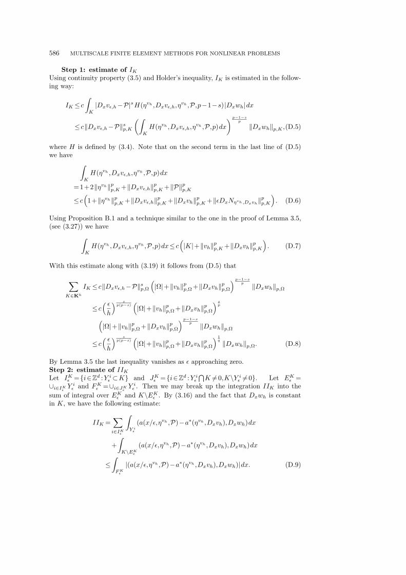
586 MULTISCALE FINITE ELEMENT METHODS FOR NONLINEAR PROBLEMS
Step 1: estimate of IK
Using continuity property (3.5) and Holder’s inequality, IK is estimated in the follow-ing way:
IK ≤ c
∫
K
|Dxvε,h−P|sH(ηvh ,Dxvε,h,ηvh ,P,p−1−s)|Dxwh|dx
≤ c‖Dxvε,h−P‖sp,K
(∫
K
H(ηvh ,Dxvε,h,ηvh ,P,p)dx
) p−1−sp
‖Dxwh‖p,K ,(D.5)
where H is defined by (3.4). Note that on the second term in the last line of (D.5)we have
∫
K
H(ηvh ,Dxvε,h,ηvh ,P,p)dx
=1+2‖ηvh‖pp,K +‖Dxvε,h‖p
p,K +‖P‖pp,K
≤ c(1+‖ηvh‖p
p,K +‖Dxvε,h‖pp,K +‖Dxvh‖p
p,K +‖εDxNηvh ,Dxvh‖p
p,K
). (D.6)
Using Proposition B.1 and a technique similar to the one in the proof of Lemma 3.5,(see (3.27)) we have
∫
K
H(ηvh ,Dxvε,h,ηvh ,P,p)dx≤ c(|K|+‖vh‖p
p,K +‖Dxvh‖pp,K
). (D.7)
With this estimate along with (3.19) it follows from (D.5) that
∑
K∈Kh
IK ≤ c‖Dxvε,h−P‖sp,Ω
(|Ω|+‖vh‖p
p,Ω +‖Dxvh‖pp,Ω
) p−1−sp ‖Dxwh‖p,Ω
≤ c( ε
h
) sp(p−s)
(|Ω|+‖vh‖p
p,Ω +‖Dxvh‖pp,Ω
) sp
(|Ω|+‖vh‖p
p,Ω +‖Dxvh‖pp,Ω
) p−1−sp ‖Dxwh‖p,Ω
≤ c( ε
h
) sp(p−s)
(|Ω|+‖vh‖p
p,Ω +‖Dxvh‖pp,Ω
) 1q ‖Dxwh‖p,Ω. (D.8)
By Lemma 3.5 the last inequality vanishes as ε approaching zero.Step 2: estimate of IIK
Let IKε =i∈Zd :Y i
ε ⊂K and JKε =i∈Zd :Y i
ε
⋂K 6=0,K\Y i
ε 6=0. Let EKε =
∪i∈IKε
Y iε and FK
ε =∪i∈JKε
Y iε . Then we may break up the integration IIK into the
sum of integral over EKε and K\EK
ε . By (3.16) and the fact that Dxwh is constantin K, we have the following estimate:
IIK =∑
i∈IKε
∫
Y iε
(a(x/ε,ηvh ,P)−a∗(ηvh ,Dxvh),Dxwh)dx
+∫
K\EKε
(a(x/ε,ηvh ,P)−a∗(ηvh ,Dxvh),Dxwh)dx
≤∫
F Kε
|(a(x/ε,ηvh ,P)−a∗(ηvh ,Dxvh),Dxwh)|dx. (D.9)

Y. EFENDIEV, T. HOU AND V. GINTING 587
It follows by applying Holder’s inequality appropriately and using Proposition 3.6that
∑
K∈Kh
IIK
≤∑
K∈Kh
∑
i∈JKε
∫
Y iε
(|(a(x/ε,ηvh ,P),Dxwh)|+ |(a∗(ηvh ,Dxvh),Dxwh)|) dx
≤ c∑
K∈Kh
∑
i∈JKε
∫
Y iε
H(ηvh ,P,ηvh ,Dxvh,p−1)|Dxwh|dx
≤ c
∑
K∈Kh
∑
i∈JKε
∫
Y iε
H(ηvh ,P,ηvh ,Dxvh,p)dx
1q
∑
K∈Kh
∑
i∈JKε
∫
Y iε
|Dxwh|pdx
1p
≤ c
∑
K∈Kh
∑
i∈JKε
(1+ |ηvh |p + |Dxvh|p) |Y iε |
1q
∑
K∈Kh
∑
i∈JKε
|Dxwh|p |Y iε |
1p
≤ c
∑
K∈Kh
|K| (1+ |ηvh |p + |Dxvh|p) |FKε ||K|
1q
∑
K∈Kh
|K||Dxwh|p |FKε ||K|
1p
≤ cmaxK
( |FKε ||K|
) 1q (|Ω|+‖vh‖p
p,Ω +‖Dxvh‖pp,Ω
) 1q
maxK
( |FKε ||K|
) 1q (‖Dxwh‖p
p,Ω
) 1p
≤ c( ε
h
)(|Ω|+‖vh‖p
p,Ω +‖Dxvh‖pp,Ω
) 1q
.‖Dxwh‖p,Ω (D.10)
This expression vanishes as ε approaches to zero.
Step 3: estimate of IIIK
Using (3.5) for the homogenized fluxes and Holder’s inequality we estimate IIIK inthe following way:
IIIK ≤ c
∫
K
H(ηvh ,Dxvh,vh,Dxvh,p−1)ν(|ηvh−vh|)|Dxwh|dx
≤ c
(∫
K
H(ηvh ,Dxvh,vh,Dxvh,p)ν(|ηvh−vh|)q dx
) 1q
‖Dxwh‖p,K . (D.11)
It follows that
∑
K∈Kh
IIIK ≤ c
(∫
Ω
H(ηvh ,Dxvh,vh,Dxvh,p)ν(|ηvh−vh|)q dx
) 1q
‖Dxwh‖p,Ω
≤ c
(∫
Ω
(|vh|p + |Dxvh|p)ν(|ηvh−vh|)q dx
) 1q
‖Dxwh‖p,Ω. (D.12)
Because Dxvh∈Lp+α(Ω), Dxwh∈Lp(Ω) and ηvh−vh converges to zero in Lp(Ω) itfollows from Lemma D.1 that
∑K∈Kh IIIK vanishes as ε→0.

588 MULTISCALE FINITE ELEMENT METHODS FOR NONLINEAR PROBLEMS
Acknowledgments. The research of Y. E. is partially supported by NSF grantsDMS-0327713 and EIA-0218229. The research of T.Y.H. is partially supported by theNSF ITR grant ACI-0204932. We would like to acknowledge anonymous reviewersfor their helpful comments which helped to improve the quality of the paper.
REFERENCES
[1] T. Arbogast, An overview of subgrid upscaling for elliptic problems in mixed form, in CurrentTrends in Scientific Computing (Xi’an, 2002), Contemp. Math., Amer. Math. Soc., Provi-dence, RI, 329, 21–32, 2003.
[2] T. Arbogast, Analysis of a two-scale, locally conservative subgrid upscaling for elliptic problems,SIAM J. Numer. Anal., 42, 2, 576-598, 2004.
[3] I. Babuska, G. Caloz and E. Osborn, Special finite element methods for a class of second orderelliptic problems with rough coefficients, SIAM J. Numer. Anal., 31, 945-981, 1994.
[4] I. Babuska and E. Osborn, Generalized finite element methods: their performance and theirrelation to mixed methods, SIAM J. Numer. Anal., 20, 510-536, 1983.
[5] F. Brezzi, Interacting with the subgrid world, in Numerical analysis 1999 (Dundee), Chapman &Hall/CRC, Boca Raton, FL, 69-82, 2000.
[6] M. A. Celia, E. T. Bouloutas and R. L. Zarba, A general mass-conservative numerical solutionfor the unsaturated flow equation, Water Resour. Res., 26, 7, 1483-1496, 1990.
[7] S.- S. Chow, Finite element error estimates for nonlinear elliptic equations of monotone type,Numer. Math., 54, 373-393, 1989.
[8] G. Dal Maso and A. Defranceschi, Correctors for the homogenization of monotone operators,Differential Integral Equations, 3, 1151-1166, 1990.
[9] C. V. Deutsch and A. G. Journel, GSLIB: Geostatistical Software Library and User’s Guide,2nd Edition, Oxford University Press, New York, 1998.
[10] W. E and B. Engquist, The heterogeneous multi-scale methods, Comm. Math. Sci., 1, 1, 87-132,2003.
[11] Y. Efendiev and A. Pankov, Homogenization of nonlinear random parabolic operators,submitted to EJDE (available at http://www.math.tamu.edu/∼yalchin.efendiev/ep-hom-parab.ps).
[12] Y. Efendiev and A. Pankov, Meyers type estimates for approximate solutions of nonlin-ear elliptic equations and their applications, submitted to Num. Math., (available athttp://www.math.tamu.edu/∼yalchin.efendiev/ep-meyers-elliptic.ps).
[13] Y. Efendiev and A. Pankov, Numerical homogenization of nonlinear random parabolic operators,SIAM Multiscale Model. and Simul., 2, 2, 237-268, 2004.
[14] Y. R. Efendiev, T. Y. Hou and X. H. Wu, Convergence of a nonconforming multiscale finiteelement method, SIAM J. Num. Anal., 37, 888 -910, 2000.
[15] A. Ern and J.-L. Guermond, Theory and Practice of Finite Elements, Applied MathematicalSciences, Springer-Verlag, New York, 159, 2004.
[16] R. Eymard, T. Gallouet and R. Herbin, Finite volume methods, in Handbook of NumericalAnalysis, Vol. VII, Handb. Numer. Anal., VII, North-Holland, Amsterdam, 713 -1020, 2000.
[17] V. Ginting, Computational Upscaled Modeling of Heterogeneous Porous Media Flows UtilizingFinite Volume Method, PhD thesis, Texas A&M University, College Station, 2004.
[18] T. Hou, X. Wu and Y. Zhang, Removing the cell resonance error in the multiscale finite elementmethod via a petrov-galerkin formulation, Comm. in Math. Sci., 2, 2, 185–205, 2004.
[19] T. Y. Hou and X. H. Wu, A multiscale finite element method for elliptic problems in compositematerials and porous media, Journal of Computational Physics, 134, 169-189, 1997.
[20] T. Y. Hou, X. H. Wu and Z. Cai, Convergence of a multiscale finite element method for ellipticproblems with rapidly oscillating coefficients, Math. Comp., 68, 913-943, 1999.
[21] T. Hughes, G. Feijoo, L. Mazzei and J. Quincy, The variational multiscale method - a paradigmfor computational mechanics, Comput. Methods Appl. Mech. Engrg, 166, 3-24, 1998.
[22] V. V. Jikov, S. M. Kozlov and O. A. Oleinik, Homogenization of Differential Operators andIntegral Functionals, Springer-Verlag, New York, 1994.
[23] M. A. Krasnosel′skiı, P. P. Zabreıko, E. I. Pustyl′nik and P. E. Sobolevskiı, Integral Operators InSpaces of Summable Functions, Noordhoff International Publishing, Leiden, 1976. (Trans-lated from the Russian by T. Ando, Monographs and Textbooks on Mechanics of Solids andFluids, Mechanics: Analysis.)
[24] J. Lions, Quelques Methodes de Resoluton des Problemes aux Limites Non Lineairies, Dunod,Paris, 1969.

Y. EFENDIEV, T. HOU AND V. GINTING 589
[25] A.-M. Matache and C. Schwab, Homogenization via p-FEM for problems with microstructure,in Proceedings of the Fourth International Conference on Spectral and High Order Methods(ICOSAHOM 1998) (Herzliya), 33, 43-59, 2000.
[26] N. G. Meyers and A. Elcrat, Some results on regularity for solutions of non-linear ellipticsystems and quasi-regular functions, Duke Math. J., 42, 121-136, 1975.
[27] J. Necas, Introduction to the Theory of Nonlinear Elliptic Equations, A Wiley-IntersciencePublication, John Wiley & Sons Ltd., Chichester, 1986. Reprint of the 1983 edition.
[28] A. Pankov, G-convergence and Homogenization of Nonlinear Partial Differential Operators,Kluwer Academic Publishers, Dordrecht, 1997.
[29] W. V. Petryshyn, On the approximation-solvability of equations involving A-proper and psuedo-A-proper mappings, Bull. Amer. Math. Soc., 81, 223-312, 1975.
[30] L. Richards, Capillary conduction of liquids through porous mediums, Physics, 318-333, 1931.[31] G. Sangalli, Capturing small scales in elliptic problems using a residual-free bubbles finite ele-
ment method, SIAM Multiscale Model. Simul., 1, 485-503, 2003 (electronic).[32] R. E. Showalter, Monotone operators in Banach space and nonlinear partial differential equa-
tions, Mathematical Surveys and Monographs, American Mathematical Society, Providence,RI, 49, 1997.
[33] I. V. Skrypnik, Methods for analysis of nonlinear elliptic boundary value problems, Translationsof Mathematical Monographs, American Mathematical Society, Providence, RI, 139, 1994.(Translated from the 1990 Russian original by Dan D. Pascali).
[34] M. T. van Genuchten, A closed-form equation for predicting the hydraulic conductivity of un-saturated soils, Soil. Sci. Soc. Am. J., 44, 892-898, 1980.
[35] A. W. Warrick, Time-dependent linearized infiltration: III. strip and disc sources, Soil. Sci.Soc. Am. J., 40, 639-643, 1976.
[36] X. Wen, L. Durlofsky and M. Edwards, Use of border regions for improved permeability upscal-ing, Mathematical Geology, 35, 521-547, 2003.
[37] E. Zeidler, Nonlinear Functional Analysis and Its Applications. II/B, Springer-Verlag, NewYork, 1990. (Nonlinear monotone operators, Translated from the German by the authorand Leo F. Boron).