a multiresolution space-time adaptive scheme for the...

A Multiresolution Space-Time Adaptive Schemefor the Bidomain Model in ElectrocardiologyMostafa Bendahmane,1 Raimund Bürger,2 Ricardo Ruiz-Baier3

1Department of Mathematics, Al-Imam University, Saudi Arabia2CI 2MA and Departamento de Ingeniería Matemática, Facultad de Ciencias Físicas yMatemáticas, Universidad de Concepción, Casilla 160-C, Concepción, Chile

3IACS, Chair of Modelling and Scientific Computing, École Polytechnique Fédérale deLausanne, Station 8, CH-1015 Lausanne, Switzerland

Received 29 September 2008; accepted 22 April 2009Published online 29 October 2009 in Wiley Online Library (wileyonlinelibrary.com).DOI 10.1002/num.20495

The bidomain model of electrical activity of myocardial tissue consists of a possibly degenerate parabolicPDE coupled with an elliptic PDE for the transmembrane and extracellular potentials, respectively. Thissystem of two scalar PDEs is supplemented by a time-dependent ODE modeling the evolution of the gatingvariable. In the simpler subcase of the monodomain model, the elliptic PDE reduces to an algebraic equation.Since typical solutions of the bidomain and monodomain models exhibit wavefronts with steep gradients, wepropose a finite volume scheme enriched by a fully adaptive multiresolution method, whose basic purpose isto concentrate computational effort on zones of strong variation of the solution. Time adaptivity is achievedby two alternative devices, namely locally varying time stepping and a Runge-Kutta-Fehlberg-type adaptivetime integration. A series of numerical examples demonstrates that these methods are efficient and suffi-ciently accurate to simulate the electrical activity in myocardial tissue with affordable effort. In addition, theoptimal choice of the threshold for discarding nonsignificant information in the multiresolution representa-tion of the solution is addressed, and the numerical efficiency and accuracy of the method is measured interms of CPU time speed-up, memory compression, and errors in different norms. © 2009 Wiley Periodicals,Inc. Numer Methods Partial Differential Eq 26: 1377–1404, 2010

Keywords: bidomain model; electrocardiology; fully adaptive multiresolution schemes; local time stepping;parabolic-elliptic system; Runge-Kutta-Fehlberg

Correspondence to: Raimund Bürger, CI2 MA and Departamento de Ingeniería Matemática, Facultad de Ciencias Físicasy Matemáticas, Universidad de Concepción, Casilla 160-C, Concepción, Chile (e-mail: [email protected])Contract grant sponsor: Fondecyt; contract grant numbers: 1070682 and 1090456Contract grant sponsor: Fondap; contract grant number: 15000001Contract grant sponsor: BASAL project CMM, Universidad de Chile and Centro de Investigación en Ingeniería Matemática(CI2MA), Universidad de ConcepciónContract grant sponsor: ERC; contract grant number: AG227058

© 2009 Wiley Periodicals, Inc.

1378 BENDAHMANE, BÜRGER, AND RUIZ-BAIER

I. INTRODUCTION

A. Scope

The obvious difficulty of direct measurements in electrocardiology early motivated interest inthe numerical simulation of cardiac models. In 1952, Hodgkin and Huxley [1] introduced thefirst mathematical model of wave propagation in squid nerve, which was modified later on todescribe several phenomena in biology, including the first physiological model of cardiac tis-sue (see [2]). Among these models, the bidomain model, first introduced by Tung [3], is oneof the most accurate and complete models for the theoretical and numerical study of the elec-tric activity in cardiac tissue. The bidomain equations result from the principle of conservationof current between the intra- and extracellular domains, followed by a homogenization process(see e.g. [2, 4, 5]) derived from a scaled version of a cellular model on a periodic structure ofcardiac tissue. Mathematically, the bidomain model is a system consisting of a scalar, possiblydegenerate parabolic PDE coupled with a scalar elliptic PDE for the transmembrane potential andthe extracellular potential, respectively. These equations are supplemented by a time-dependentODE for the gating variable, which is defined at every point of the spatial computational domain.The term “bidomain” reflects that, in general, the intra- and extracellular tissues have differentlongitudinal and transversal (with respect to the fiber) conductivities; if these are equal, then themodel is termed monodomain model, and the elliptic PDE reduces to an algebraic equation. Thedegenerate nature of the bidomain model is essentially due to the differences between the intra-and extracellular anisotropy of the cardiac tissue [4, 6].

The bidomain model is a challenge for computation since the width of an excitation front isroughly two orders of magnitude smaller than the long axis of a human-size right ventricle. Thisfeature of localization, along with strongly varying time scales in the reaction terms, producessolutions with sharp propagating wave fronts in the potential field, which almost precludes simu-lations with uniform grids. Clearly, cardiac simulations should be based on space- (and also time-)adaptive methods.

It is the purpose of this article to advance a fully adaptive multiresolution (MR) scheme withlocally varying space-time stepping (LTS) and adaptive time step control by means of a Runge-Kutta-Fehlberg (RKF) method for the numerical solution of the bidomain and monodomainmodels. The LTS and RKF strategies are of different nature, but may be combined to obtaina potentially more powerful method (as suggested, e.g., in [7]; however, herein we do not pursuethis). We furthermore deduce an optimal threshold value for discarding nonsignificant data, whichpermits to achieve significant data compression. This deduction motivated by the rigorous analy-sis performed in [8] for scalar conservation laws in one space dimension and in [9] for strictlyparabolic PDEs. Experience with degenerate parabolic equations and reaction–diffusion systems[9–12] suggests that the MR method should provide an efficient tool for solving the bidomainequations. Consequently, we herein extend this method to the novel application of the bidomainand monodomain models.

The efficiency of the MR method is a consequence of the fact that, at each time step, the solu-tion is encoded with respect to a MR basis corresponding to a hierarchy of nested grids. The sizeof the details determines the level of refinement needed to obtain an accurate local representationof the solution. Therefore, an adaptive mesh is evolved in time by refining and coarsening in asuitable way, by means of a strategy based on the prediction of the displacement and creation ofsteep gradients and similar singularities in the solution.

We apply the MR approach to an explicit finite volume (FV) method in each time step. Eventhough implicit methods allow larger time steps, we need to iteratively solve a nonlinear sys-tem in each time step, using e.g., Newton-Raphson method. The number of iterations is usually

Numerical Methods for Partial Differential Equations DOI 10.1002/num

MULTIRESOLUTION SCHEME FOR THE BIDOMAIN MODEL 1379

controlled by measuring the residual error and cannot be controlled a priori. Thus, it appearsdifficult to assess the true benefits of a time-stepping strategy if the basic time discretization is animplicit one, the latter being less efficient than explicit ones, especially when the overall numberof time steps is large (see e.g., [13]).

B. Related Work

We first mention that standard theory for coupled parabolic–elliptic systems (see e.g., [14]) doesnot apply naturally to the bidomain equations, since the anisotropies of the intra- and extracel-lular media differ and the resulting system is of degenerate parabolic type. Colli Franzone andSavaré [6] present a weak formulation for the bidomain model and show that it has a structure suit-able for applying the theory of evolution variational inequalities in Hilbert spaces. Bendahmaneand Karlsen [4] prove existence and uniqueness for the bidomain equations using the Faedo-Galerkin method and compactness theory for the existence part, and Bourgault et al. [15] proveexistence and uniqueness for the bidomain equations by first reformulating the problem as a singleparabolic PDE and then applying a semigroup approach.

From a computational point of view, substantial contributions have been made in adaptivity forcardiac models. However, our treatment differs to the best of our knowledge from other adaptiveapproaches in the literature, which include adaptive mesh refinement (AMR) (e.g., [13]), adap-tive finite element methods using a posteriori error techniques (see e.g., [5]) or multigrid methodsapplied to finite elements. Furthermore, Quan et al. [16] present a domain decomposition approachusing an alternating direction implicit (ADI) method. Sundnes et al. [17] introduce an operatorsplitting method to solve a fully coupled discretization of three PDEs modelling the interactionbetween the myocardium and the torso surrounding the heart. With respect to time adaptivity,Skouibine et al. [18] present a predictor–corrector time stepping strategy to accelerate a givenfinite difference scheme for the bidomain equations using active membrane kinetics (Luo-Rudyphase II). Cherry et al. [13] use local time stepping, similar to the method introduced by Bergerand Oliger [19], to accelerate a reference scheme. Parallelized versions of part of the methodsmentioned earlier are presented, for example, by Colli Franzone and Pavarino [20] and Saleheenand Ng [21].

MR schemes for hyperbolic partial differential equations were first proposed by Harten [22].We refer to Müller [23] for a survey on MR methods, see also Chiavassa et al. [24], and Cohenet al. [8] and Dahmen et al. [25] for the application of classical MR methods to hyperbolic partialdifferential equations.

The aim of the MR method is to accelerate a given reference discretization scheme while con-trolling the error. In the context of fully adaptive MR methods [8], the mathematical analysis iscomplete only in the case of a scalar conservation law, but in practice, these techniques have beenused by several groups (see e.g., [7, 9, 10, 23, 26]) to successfully solve a wide class of problems,including applications to multidimensional systems. These results illustrate that the MR methodhas turned out to be a useful device for a series of problems with a similar structure to cardiacproblems. Thus, our motivation is to point out that this versatile method also provides an efficienttool for the simulation of electrical activity in cardiac tissue.

C. Outline of the Article

The remainder of this article is organized as follows. In Section II, the bidomain and monodomainmodels of cardiac tissue are outlined. Section III deals with the construction of an appropriate FVmethod for the solution of both the parabolic–elliptic system and the reaction–diffusion equation



arising from the bidomain and monodomain models, respectively. Next, in Section IV, we developthe MR analysis used to endow the reference FV schemes with space adaptivity. More precisely, inSection IVA, we introduce the wavelet basis underlying the MR representation with the pertinentprojection operator. In Section IVB, the prediction operator, the detail coefficients and the thresh-olding procedure are introduced. In Section IVC, we recall the graded tree data structure used forstorage of the numerical solution, and which is introduced for ease of navigation. In Section IVD,we first recall the results of the rigorous error analyses of Cohen et al. [8] and Roussel et al. [9]referring to conservation laws and strictly parabolic equations, respectively, and then show howthis analysis motivates the choice of a reference tolerance εR for the bidomain and monodomainmodels in a fashion similar to the treatment of scalar degenerate parabolic equations [11, 12].The quantity εR determines the comparison values εl used for the thresholding operation at eachlevel l of resolution. Overall, the basic goal is to choose the threshold values in such a way thatthe resulting MR scheme has the same order of accuracy as the usual FV scheme.

In Section V, we address two strategies for the adaptive evolution in time of the space-adaptiveMR scheme, namely the locally varying time stepping (LTS, Section VA) and a variant ofthe well-known Runge-Kutta-Fehlberg (RKF, Section VB) method. Finally, in Section VI, wepresent numerical examples putting into evidence the efficiency of the underlying methods. Someconclusions of the article are given in Section VII.

II. THE MACROSCOPIC BIDOMAIN AND MONODOMAIN MODELS

We consider a bounded open subset � ⊂ R2 with a piecewise smooth boundary ∂�. The domain

� represents a slice of the cardiac muscle regarded as two interpenetrating and superimposed(anisotropic) continuous media, namely the intracellular (i) and extracellular (e) tissues. Thesetissues occupy the same two-dimensional area, and are separated from each other (and connectedat each point) by the cardiac cellular membrane. The quantities of interest are intracellular andextracellular electric potentials, ui = ui(x, t) and ue = ue(x, t), at (x, t) ∈ �T := � × (0, T ).Their difference v = v(x, t) := ui − ue is the transmembrane potential. The conductivity of thetissue is represented by scaled tensors Mi(x) and Me(x) given by

Mk(x) = σ tkI + (

σ lk − σ t

k

)al(x)aT

l (x), k ∈ {e, i},where σ l

k = σ lk(x) ∈ C1(R2) and σ t

k = σ tk(x) ∈ C1(R2), k ∈ {e, i}, are the intra- and extracellular

conductivities along and transversal to the direction of the fiber (parallel to the unitary directionvector denoted by al(x)), respectively, and aT

l (x) is the transpose of al(x). For fibers aligned withthe axis, Mi(x) and Me(x) are diagonal matrices: Mi(x) = diag(σ l

i , σ ti ) and Me(x) = diag(σ l

e , σ te).

When the anisotropy ratios σ li /σ

ti and σ l

e/σte are equal, we are in the case of equal anisotropy, and

the case where the conductivities in the longitudinal direction l are higher than those across thefiber (transversal direction t) is called strong anisotropy of electrical conductivity. When the fibersrotate from bottom to top, this type of anisotropy is often referred to as rotational anisotropy.

The bidomain model is given by the following coupled reaction–diffusion system (seee.g., [27]):

βcm∂tv − ∇ · (Mi(x)∇ui

) + βIion(v, w) = 0, (2.1a)

βcm∂tv + ∇ · (Me(x)∇ue

) + βIion(v, w) = Iapp, (2.1b)

∂tw − H(v, w) = 0, (x, t) ∈ �T . (2.1c)



Here, cm > 0 is the surface capacitance of the membrane, β is the surface-to-volume ratio, andw(x, t) is the gating or recovery variable. The stimulation currents applied to the extracellularspace are represented by the function Iapp = Iapp(x, t). The functions H(v, w) and Iion(v, w)

correspond to the fairly simple Mitchell-Schaeffer membrane model [28] for the membrane andionic currents:

H(v, w) = w∞(v/vp) − w

Rmcmη∞(v/vp), Iion(v, w) = vp

Rm

(v

vpη2− v2(1 − v/vp)w

v2pη1

), (2.2)

where η∞(s) = η3 + (η4 −η3)H(s −η5) and w∞(s) = H(s −η5), where H denotes the Heavisidefunction, Rm is the surface resistivity of the membrane, and vp and η1, . . . , η5 are given parame-ters. A simpler choice for the membrane kinetics is the well-known FitzHugh-Nagumo model(see [2]), which is specified by

H(v, w) = av − bw, Iion(v, w) = −λ(w − v(1 − v)(v − θ)

), (2.3)

where a, b, λ, and θ are given parameters.We rewrite (2.1) as the strongly coupled parabolic–elliptic PDE-ODE system (see e.g., [27])

βcm∂tv + ∇ · (Me(x)∇ue

) + βIion(v, w) = Iapp, (2.4a)

∇ · ((Mi(x) + Me(x))∇ue

) + ∇ · (Mi(x)∇v

) = Iapp, (2.4b)

∂tw − H(v, w) = 0, (x, t) ∈ �T . (2.4c)

We utilize zero flux boundary conditions corresponding to an isolated piece of cardiac tissue,

(Mk(x)∇uk

) · n = 0 on T := ∂� × (0, T ), k ∈ {e, i}, (2.5)

and impose initial conditions (which are degenerate for the transmembrane potential v):

v(0, x) = v0(x), w(0, x) = w0(x), x ∈ �. (2.6)

We require the initial datum v0 to be compatible with (2.5) in the following sense. If we fix bothuk(0, x), k ∈ {e, i} as initial data, the problem may become unsolvable, since the time derivativeinvolves only v = ui − ue (this is also referred as degeneracy in time). Thus, we impose thecompatibility condition ∫

�

ue(x, t) dx = 0 for a.e. t ∈ (0, T ). (2.7)

In the case that Mi ≡ µMe for some constant µ ∈ R, the system (2.1) is equivalent to a scalarparabolic equation for v, coupled to an ODE for w. This parabolic equation is obtained by multi-plying (2.1a) by 1/(1 + µ), (2.1b) by µ/(1 + µ), and adding the results. The final monodomainmodel can be stated as follows:

βcm∂tv − ∇ ·(

Mi

1 + µ∇v

)+ βIion(v, w) = µ

1 + µIapp,

∂tw − H(v, w) = 0, (x, t) ∈ �T . (2.8)



This simpler model requires less computational effort than (2.4), and even though the assumptionof equal anisotropy ratios is very strong and generally unrealistic, (2.8) is adequate for a qualita-tive investigation of repolarization sequences and the distribution of patterns of durations of theaction potential [29].

We assume that the functions Me, Mi, Iion, and H are sufficiently smooth so that the follow-ing definitions of weak solutions make sense. Furthermore, we assume that Iapp ∈ L2(�T ) andMk ∈ L∞(�) and Mkξ · ξ ≥ CM |ξ |2 for a.e. x ∈ �, for all ξ ∈ R

2, k ∈ {e, i}, and a constantCM > 0. For the sake of completeness, we state the definitions of a weak solution for the bidomainand the monodomain model, respectively.

Definition 2.1. A triple u = (v, ue, w) of functions is a weak solution of the bidomain model(2.4)–(2.6) if v, ue ∈ L2(0, T ; H 1(�)), w ∈ C([0, T ], L2(�)), (2.7) is satisfied, and the followingidentities hold for all test functions ϕ, ψ , ξ ∈ D([0, T ) × �):

βcm

∫�

v0(x)ϕ(0, x) dx +∫∫

�T

{βcmv∂tϕ − Me(x)∇ue · ∇ϕ + βIionϕ

}dx dt

=∫∫

�T

Iappϕ dx dt ,

∫∫�T

{−(

Mi(x) + Me(x))∇ue · ∇ψ − Mi(x)∇v · ∇ψ

}dx dt =

∫∫�T

Iappϕ dx dt ,

−∫

�

w0(x)ξ(0, x) dx −∫∫

�T

w∂tξ dx dt =∫∫

�T

Hξ dx dt .

Definition 2.2. A pair u = (v, w) of functions is a weak solution of the monodomain model(2.8) if v ∈ L2(0, T ; H 1(�)), w ∈ C([0, T ], L2(�)), and the following identities hold for all testfunctions ϕ, ξ ∈ D([0, T ) × �):

βcm

∫�

v0(x)ϕ(0, x) dx +∫∫

�T

{βcmv∂tϕ + βIionϕ − 1

1 + µMi∇v · ∇ϕ

}dx dt

= µ

1 + µ

∫∫�T

Iappϕ dx dt ,

−∫

�

w0(x)ξ(0, x) dx −∫∫

�T

w∂tξ dx dt =∫∫

�T

Hξ dx dt .

III. THE REFERENCE FINITE VOLUME SCHEME

To approximate solutions to the bidomain equations (2.4), we employ a standard FV scheme,which is described here for a uniform grid. The square spatial domain � ⊂ R

2 is partitioned intocontrol volumes (�ij )1≤i,j≤N , where we define

�ij := [xi−1/2, xi+1/2] × [yj−1/2, yj+1/2]and h := xi+1/2 − xi−1/2 = yj+1/2 − yj−1/2 for all 1 ≤ i, j ≤ N . We also choose a time step size t > 0 and set tn := n t for n ∈ {0, . . . , N ′}, where N ′ > 0 is the smallest integer such thatN ′ t ≥ T . The cell average of a quantity q over �ij at time tn is defined by



qnij := 1

h2

∫∫�ij

q(x, tn) dx dt .

We define the unknowns

Hnij := H

(vn

ij , wnij

), I n

ion,(i,j) := Iion

(vn

ij , wnij

), (3.1)

and the cell averages of the given function Iapp at time tn:

I napp,(i,j) := 1

h2

∫∫�ij

Iapp(x, tn) dx dt .

Denoting by θ the angle of alignment of the fibers, we may recast Mk(x) explicitly in the form(see e.g. [30])

Mk =[

σ tk + (σ l

k − σ tk) sin2(θ) (σ l

k − σ tk) sin(θ) cos(θ)

(σ lk − σ t

k) sin(θ) cos(θ) σ tk + (σ l

k − σ tk) cos2(θ)

]for k ∈ {e, i}.

Therefore, defining the difference operators δsxVij := Vi+s,j − Vij and δs

yVij := Vi,j+s − Vij , wedefine the numerical fluxes (we only provide those corresponding to the flux (i + 1, j) → (i, j))

Fu,e(i+1,j)→(i,j) := 1

hM11

e δ1xue,(i,j),

Fu,i,e(i+1,j)→(i,j) := 1

h

(M11

e + M11i

)δ1xue,(i,j),

Fv,i(i+1,j)→(i,j) := 1

hM11

i δ1xvij ,

and following e.g., [21], the corresponding anisotropic diffusive term may be approximated by

∇ · (Mk∇u)i,j ≈ Dh(Mk , uij ) := 1

h2

∑s∈{−1,1}

M11k δs

xuij + M12k ui+s,j+s + M21

k ui+s,j−s + M22k δs

yuij

for all 1 ≤ i, j ≤ N and k ∈ {e, i}. We now describe the finite volume scheme employed toadvance the numerical solution from tn to tn+1, which is based on a simple explicit Euler timediscretization. The computation starts from the initial cell averages

v0ij = 1

h2

∫�ij

v0(x) dx, w0ij = 1

h2

∫�ij

w0(x) dx. (3.2)

Now, we first integrate the corresponding equations, average over �ij and discretize.Then, assuming that at t = tn the quantities un

k,(i,j), k ∈ {e, i}, vnij and wn

ij are known for all �ij ,we compute their new values at t = tn+1, un+1

k,(i,j), k ∈ {e, i}, vn+1ij and wn+1

ij , from

βcm

vn+1ij − vn

ij

t+ Dh

(Me, u

ne,(i,j)

) + βInion,(i,j) = I n

app,(i,j), (3.3)

Dh

((Me + Mi), u

n+1e,(i,j)

) + Dh

(Mi, v

n+1ij

) = I napp,(i,j), (3.4)

wn+1ij − wn

ij

t− Hn

ij = 0. (3.5)



The boundary condition (2.5) is taken into account by imposing zero fluxes on the externaledges (which we only show here for the right boundary of a square domain):

Fu,e(i,N)→(i,N−1) ≡ 1

hM11

e δ1xue,(i,N−1) = 0,

Fu,i,e(i,N)→(i,N−1) ≡ 1

h

(M11

e + M11i

)δ1xue,(i,N−1) = 0

for 1 ≤ i ≤ N − 1, and the compatibility condition (2.7) is discretized via

N∑i,j=1

h2une,(i,j) = 0, n = 0, 1, 2, . . . .

Analogously, a FV method for the monodomain model (2.8) is given by (3.2) and the followingformulas to advance the solution over one time step:

βcm

vn+1ij − vn

ij

t+ Dh

(1

1 + µMi, v

nij

)+ βIn

ion,(i,j) = µ

1 + µIn

app,(i,j),

wn+1ij − wn

ij

t− Hn

ij = 0.

A FV method on arbitrary meshes for a different version of the bidomain equations is analyzedin [31]. In that article, the authors prove existence and uniqueness of solutions to an implicit FVscheme, and provide convergence results. On the other hand, following [31,32], we prove in [33]existence and uniqueness of approximate solutions (that is, well-definedness of the scheme) foran implicit FV method on rectangular meshes, and show that it converges to the correspondingweak solution for the monodomain problem, and also for the bidomain equations in the specialcase when Mi and Me are diagonal tensors.

Moreover, as in [10], we may deduce that the explicit version of the FV method used herein,(3.2)–(3.5), is stable under the CFL condition

t ≤ h

(2 max

1≤i,j≤N

(∣∣I nion,(i,j)

∣∣ + ∣∣I napp,(i,j)

∣∣) + 4h−1 max1≤i,j≤N

(∣∣Mi,(i,j)

∣∣ + ∣∣Me,(i,j)

∣∣))−1

. (3.6)

Note that the values of I nion,(i,j) and I n

app,(i,j) depend on time. Since Iapp is a given control function,max1≤i,j≤N |I n

app,(i,j)| can assumed to be bounded, but I nion,(i,j) is not bounded a priori for arbitrarily

large times. Consequently, in our computations, we evaluate the right-hand side of (3.6) after eachiteration at t = tn, and use (3.6) to define the time step size t to advance the solution from tn totn+1 = tn + t .

The following algorithm shows how the solution un+1 = (v, ue, w)n+1 is obtained in each timestep

Algorithm 3.1 Time discretization.

1. Assume that uni , un

e , vn and wn are known (at time tn).2. Compute wn+1 using

wn+1 − wn

t− H(vn, wn) = 0.



3. Calculate vn+1 by solving

βcmvn+1 − vn

t+ Dh

(Me, u

ne

) + βIion(vn, wn) = I n

app.

4. Calculate un+1e from the linear system

Dh

((Me + Mi), u

n+1e

) + Dh

(Mi, v

n+1) = I n

app.

This algorithm structure is usually preferred for systems involving parabolic and ellipticequations, since it explicitly isolates the solution of the elliptic problem from the rest of thecomputations [34].

IV. MULTIRESOLUTION AND WAVELETS

A. Wavelet Basis

Consider a rectangle which after a change of variables can be regarded as � = [0, 1]2. We deter-mine a nested mesh hierarchy �0 ⊂ · · · ⊂ �L, using a uniform dyadic partition of �. Here eachgrid �l := {V(i,j),l}(i,j), with (i, j) to be defined, is formed by the control volumes on each level

V(i,j),l := [2−l i, 2−l(i + 1)

] × [2−lj , 2−l(j + 1)

],

i, j ∈ Il = {0, . . . , 2l − 1}, l = 0, . . . , L.

where l = 0 corresponds to the coarsest and l = L to the finest level, which is fixed and chosenlarge enough at the beginning of the process. The nestedness of the grid hierarchy is made preciseby the refinement sets M(i,j),l = {2(i, j) + e}, e ∈ E := {0, 1}2, which satisfy #M(i,j),l = 4. Forx = (x1, x2) ∈ V(i,j),l the scale box function is defined as

ϕ(i,j),l(x) := 1

|V(i,j),l|χV(i,j),l (x) = 22lχ[0,1]2(2lx1 − i, 2lx2 − j),

and the average of any function u(·, t) ∈ L1(�) for the cell V(i,j),l may be expressed as the innerproduct

u(i,j),l := ⟨u, ϕ(i,j),l

⟩L1(�)

.

We are now ready to define the following two-level relation for cell averages and box functions:

ϕ(i,j),l =∑

r∈M(i,j),l

|Vr,l+1||V(i,j),l| ϕr,l+1 = 1

4

∑(p,q)∈E

ϕ(2i+p,2j+q),l+1,

u(i,j),l =∑

r∈M(i,j),l

|Vr,l+1||V(i,j),l|ur,l+1 = 1

4

∑(p,q)∈E

u(2i+p,2j+q),l+1, (4.1)

which defines a projection operator, which allows us to move from finer to coarser levels. Forx ∈ V2(i,j)+a,l+1 with a ∈ E, we define the wavelet function depending on the box functions on afiner level

ψ(i,j),e,l :=∑a∈E

2−2(−1)a·eϕ2(i,j)+a,l+1 =∑

r∈M(i,j),l

|Vr=2(i,j)+a,l+1||V(i,j),l| (−1)a·eϕr,l+1.



The number of related wavelets is #M(i,j),l − 1 = 3. Since r · e ∈ {0, 1, 2} for r, e ∈ E, wehave for instance that

ψ(i,j),(1,0),l = 1

4

(ϕ2(i,j),l+1 + ϕ2(i,j)+(0,1),l+1 − ϕ2(i,j)+(1,0),l+1 − ϕ2(i,j)+(1,1),l+1

).

Doing this for all e ∈ E∗ := E \ {(0, 0)} yields an inverse two-level relation (see [23]), namely

ϕ2(i,j)+a,l+1 =∑e∈E

(−1)a·eψ(i,j),e,l , a ∈ E.

This equation is related to the concept of stable completions [23]. Roughly speaking, the L∞-counterparts of the wavelet functions {ψ(i,j),l}i,j∈Il

form a completion of the L∞-counterpart ofthe basis system {ϕ(i,j),l}i,j∈Il

, and this determines the existence of a biorthogonal system.

B. Detail Coefficients

For e ∈ E∗, we introduce the details, which will be crucial to detect zones with steep gradients:

d(i,j),e,l := ⟨u, ψ(i,j),e,l

⟩.

These detail coefficients also satisfy a two-level relation, namely

d(i,j),e,l = 1

4

∑2(i,j)+a∈M(i,j),l

(−1)a·eu2(i,j)+a,l+1. (4.2)

An appealing feature is that we can determine a transformation between the cell averages on levelL and the cell averages on level zero plus a series of details. This can be achieved by applyingrecursively the two-level relations (4.1) and (4.2); but, we also require this transformation to bereversible:

u(i,j),l+1 =∑

r∈Sl(i,j)

gl(i,j),rur,l , Sl

(i,j) := {V([i/2]+r1,[j/2]+r2),l

}r1,r2∈{−s,...,0,...,s}, (4.3)

where Sl(i,j) is the stencil of interpolation or coarsening set, gl

(i,j),r are coefficients, and the tildeover u in the left-hand side of (4.3) means that this quantity corresponds to a predicted value.

Relation (4.3) defines the so-called prediction operator, which allows us to move from coarserto finer resolution levels. In contrast to the projection, the prediction operator is not unique, butwe will impose two constraints: to be consistent with the projection, in the sense that the predic-tion operator is the right inverse of the projection operator, and to be local, in the sense that thepredicted value depends only on Sl

(i,j). For the sake of notation, in our case we may write (4.3) as

u(2i+e1,2j+e2),l+1 = u(i,j),l − (−1)e1Qx − (−1)e2Qy + (−1)e1e2Qxy ,

where e1, e2 ∈ {0, 1} and

Qx :=s∑

n=1

γn

(u(i+n,j),l − u(i−n,j),l

), Qy :=

s∑p=1

γp

(u(i,j+p),l − u(i,j−p),l

),

Qxy :=s∑

n=1

γn

s∑p=1

γp

(u(i+n,j+p),l − u(i+n,j−p),l − u(i−n,j+p),l + u(i−n,j−p),l

).



Here the corresponding coefficients are γ1 = − 22128 and γ2 = 3

128 (see [9]).From [25], we know that details are related to the regularity of a given function: if u is

sufficiently smooth, then its detail coefficients decrease when going from coarser to finer levels:∣∣du(i,j),l

∣∣ ≤ C2−2lr∥∥∇(r)u

∥∥L∞(V(i,j),l )

,

where r = 2s + 1 is the number of vanishing moments of the wavelets. This means that the moreregular u is over V(i,j),l , the smaller is the corresponding detail coefficient, so it is natural to attemptto compress data by discarding the information corresponding to small details. This thresholdingprocedure basically consists in discarding all control volumes corresponding to details that aresmaller in absolute value than a level-dependent tolerance εl ,∣∣du

(i,j),l

∣∣ < εl , l = 0, . . . , L.

Given a reference tolerance εR, whose choice is motivated in Section D, we determine εl by

εl = 22(l−L)εR, l = 0, . . . , L. (4.4)

For multicomponent solutions, there are many possible definitions for a scalar detail d(i,j),l thatis calculated from the details of the components (see a brief discussion in [11]). To guarantee thatthe refinement and coarsening procedures are always on the safe side, in the sense that we alwaysprefer to keep a node with a detail triple containing at least one component above the threshold(4.4), we will use

du(i,j),l = min

{∣∣dv(i,j),l

∣∣, ∣∣due(i,j),l

∣∣, ∣∣dw(i,j),l

∣∣}and

du(i,j),l = max

{∣∣dv(i,j),l

∣∣, ∣∣due(i,j),l

∣∣, ∣∣dw(i,j),l

∣∣}for the refinement and coarsening procedures, respectively. In practice, these details are computedsimply as the differences between the “exact” and the predicted value:

du(i,j),l := u(i,j),l − u(i,j),l .

C. Graded Tree Data Structure

We organize the cell averages and corresponding details at different levels in a dynamic gradedtree (see Fig. 1): whenever a node is included in the tree, all other nodes corresponding to thesame spatial region in coarser resolution levels are also included, and neighboring cells will differby at most one refinement level. This choice guarantees the stability of the multilevel operations[8]. We denote by root the basis of the tree. In two space dimensions, a parent node has foursons, and the sons of the same parent are called brothers. A node without sons is called a leaf.A given node has s ′ = 2 nearest neighbors in each spatial direction, needed for the computationof the fluxes of leaves; if these nearest neighbors do not exist, we create them as virtual leaves.Brothers are also considered nearest cousins. The leaves of the tree are the control volumes fromwhich we form the adaptive mesh. Here, the property of the tree being graded means that gridrefinement and coarsening is governed by that two neighboring control volumes cannot differ by



FIG. 1. A graded tree of two resolution levels. On the fine level: leaves (gray) and virtual leaves (dashedlines). On the coarse level: a parent node with its neighbors (dotted lines).

more than one level in the tree. This is equivalent to the concept of the “one-irregular” rule (seee.g., [35]). We denote by � the set of all nodes of the tree and by L(�) the restriction of � tothe leaves. We apply this MR representation to the spatial part of the function u = (v, ue, w),which corresponds to the numerical solution of the underlying problem for each time step, so weneed to update the tree structure for the proper representation of the solution during the evolution.To this end, we apply a thresholding strategy, but always keep the graded tree structure of thedata. Once the thresholding is performed, we add to the tree a safety zone, so the new tree maycontain the adaptive mesh for the next time step. The safety zone is generated by adding one finerlevel to the tree in all possible nodes without violating the graded tree data structure. This device,first proposed by Harten [22], ensures that the graded tree adequately represents the solution inthe next time step, and its effectiveness depends strongly on the assumption of finite propagationspeed of sharp fronts.

Let us now suppose that the tree has only two levels l and l + 1. (The reasoning based on thisassumption is straightforwardly extensible to an arbitrarily larger tree.) To ensure conservativityof the scheme, we compute only the fluxes at level l + 1 and we set the ingoing flux on the leaf atlevel l equal to the sum of the outgoing fluxes on the leaves of level l + 1 sharing the same edge

F(i+1,j),l→(i,j),l = F(2i+1,2j),l+1→(2i+2,2j),l+1 + F(2i+1,2j+1),l+1→(2i+2,2j+1),l+1. (4.5)

It is known that this choice decreases the number of costly flux evaluations without loosing theconservativity in the flux computation, and this represents a real advantage when using a gradedtree structure, see e.g., [9] for more details. This advantage is lost for a non-graded tree structure,for which fluxes for leaves on an immediately finer level are not always available.

The data compression rate [11, 12] η := N /(2−2LN + #L(�)) measures the improvement indata compression. Here, N is the number of control volumes in the full finest grid at level L, and#L(�) is the number of leaves. The speed-up V between the CPU time of the numerical solutionobtained by the FV method and the CPU time of the numerical solution obtained by the MRmethod is defined by V := CPU timeFV/CPU timeMR.



D. Selection of the Threshold Parameter

Error Analysis for Conservation Laws and Strictly Parabolic Equations. Let us recallthe main results of the error analysis conducted in [8] and [9] for scalar, one-dimensional conser-vation laws and strictly parabolic equations, respectively. These results rely on certain propertiesof the respective (explicit) reference FV schemes, such as the CFL stability condition, the contrac-tion property in L1 norm and an order of convergence. We decompose the global error betweenthe cell average values of the exact solution vector at the level L, denoted here by uL

ex, and thoseof the MR computation with a maximal level L, denoted by uL

MR, into two errors:∥∥uLex − uL

MR

∥∥ ≤ ∥∥uLex − uL

FV

∥∥ + ∥∥uLFV − uL

MR

∥∥. (4.6)

The first term on the right-hand side, called discretization error, refers to the FV scheme on a uni-form grid at the finest level L. For both a scalar, one-dimensional conservation law and a strictlyparabolic equation, the order of convergence, denoted by α, of the corresponding reference FVscheme is known (α = 1/2 and α = 2, respectively), which permits to obtain the estimate∥∥uL

ex − uLFV

∥∥ ≤ C12−αL (4.7)

for a constant C1 > 0. For the second term in the right-hand side of (4.6), called perturbationerror, Cohen et al. [8] assume that the details on a level l are deleted when they are smaller than aprescribed tolerance εl . Then they show that if the discrete time evolution operator is contractivein the chosen norm, and if εl is given by (4.4), then the perturbation error accumulates in timeand satisfies ‖uL

FV − uLMR‖ ≤ C2nε, where C2 > 0 and n denotes the number of time steps. At a

fixed time T = n t , this gives

∥∥uLFV − uL

MR

∥∥ ≤ C2T

tε, C2 > 0. (4.8)

For the equations considered in [8, 9], the reference FV scheme converges under the CFL-typecondition

t ≤ h2

ph + q, (4.9)

where the constants p and q depend on the coefficients of the equation under consideration, andh is the meshwidth of the finest grid, i.e., h = C(�)2−L, where C depends on the dimension andshape of the computational domain. Consequently, if t denotes the largest time step possible,then this quantity can be expressed in terms of 2−L if we consider equality in (4.9), i.e.,

t = [C(�)]22−2L

C(�)2−Lp + q. (4.10)

It is desirable to choose the level-dependent thresholds in such a way that the total error, i.e.,the error between the exact solution and the adaptive solution that is projected to the reference finemesh, remains of the same order as the discretization error. For this purpose, one has to balancethe discretization error and the perturbation error, which means that these two errors should be ofthe same order as h, or equivalently L varies. To derive an expression for ε from this requirement,we observe that the right-hand sides of (4.7) and (4.8) must be proportional, or equivalently,

ε ∝ 2−αL t . (4.11)



In light of (4.9), this yields a proportionality of the type

ε = C2−αL [C(�)]22−2L

C(�)2−Lp + q, (4.12)

from which one may deduce a value of the reference tolerance εR = ε, provided that the factorof proportionality C can be determined, for example from suitable experiments, as is done in [9].

Reference Tolerance for the Bidomain System. The previous derivation of the referencetolerance is supported by a rigorous analysis only in those cases where the order of conver-gence α is known, and the discrete time evolution operator is contractive in the chosen norm.These properties hold for a scalar, one-dimensional first-order conservation law and a second-order parabolic equation studied in the references given above. For finite volume discretizationsof the bidomain and monodomain models, however, an exact rate of convergence has not yet beenderived. Nevertheless, in [10–12] we demonstrate that also for degenerate parabolic equationsand reaction-diffusion systems, an equation of the type (4.12) may be employed to determine εR.We apply the same methodology to determine a reference tolerance for the problem at hand.On the basis of preliminary numerical experiments (obtained in a similar fashion as in [11]), forour examples, we obtained the approximate value α = 1.09, which stands for the experimentalaccuracy order of the FV reference scheme. Using this, the global CFL condition of the referenceFV scheme (3.6), the fact that h = |�|1/22−L, and the requirement that the proportionality (4.11)should hold, we obtain the following analog of (4.10):

εR = C2−(α+2)L

(|�| max

(i,j ,l)∈L(�)

(∣∣Iion,(i,j)

∣∣ + 2∣∣Iapp,(i,j)

∣∣)

+ |�|3/222+L max(i,j ,l)∈L(�)

(∣∣Mi,(i,j ,l)

∣∣ + ∣∣Me,(i,j ,l)

∣∣))−1

, (4.13)

which will give the so-called reference tolerance to be used for the numerical examples inSection VI. To determine an acceptable value for the factor C, a series of computations withdifferent tolerances are needed in each case, prior to final computations. Essentially, we selectthe largest available candidate value for C such that the same order of accuracy (same slopesfor the error computation) as that of the reference FV scheme is maintained. In [7], the authorsprove for scalar, one-dimensional nonlinear conservation laws, that the threshold error is stablein the sense that the constant C is uniformly bounded and, in particular, does not depend on thethreshold value εR, the number of refinement levels L and the number of time steps n. In ourcase, even when a rigorous proof is still missing for the system considered in the present work,from the previous deduction and our numerical experiments (see Fig. 2 in Section VI) we see asimilar behaviour for C. As in previous works [8,10–12], here the reference tolerance εR remainsfixed for all times. It is certainly possible to recompute εR at each time step, but this will usuallymean that one has to perform additional computations to determine the value of C, and it seemsunlikely that this procedure makes the scheme more efficient.

To measure errors between a reference solution u and an approximate solution uMR obtainedusing MR, we will use Lp-errors: ep = ‖un − un

MR‖p, p = 1, 2, ∞, where

e∞ = max1≤i,j≤N

∣∣uni,j − un

MR i,j ,L

∣∣; ep =(

1

N 2

N∑i,j=1

∣∣uni,j − un

MR i,j ,L

∣∣p)1/p

, p = 1, 2.



FIG. 2. Example 2 (bidomain model): data compression rate η (left), speed-up factor V (middle) andL1-errors for different levels L and values of εR (right), at t = 2.0 ms.

where unMR i,j ,L is the value on the finest level L obtained by prediction from the corresponding

leaf, and N is the number of control volumes in the finest mesh at level L in the x and y−direction,i.e., N 2 = N .

V. TIME-STEP ACCELERATING METHODS

A. Local Time Stepping

We use a version of the locally varying time stepping strategy introduced by Müller and Stiriba[26] and summarize here its principles. The basic idea is to enforce a local CFL condition byusing the same CFL number for all levels, and evolving all leaves on level l using the local timestep size

tl = 2L−l t , l = L − 1, . . . , 0,

where t = tL corresponds to the time step size on the finest level L. This strategy allows toincrease the time step for the major part of the adaptive mesh without violating the CFL stabilitycondition. The synchronization of the time stepping for the portions of the solution lying on differ-ent resolution levels will be automatically achieved after 2l time steps using tl . To additionallysave computational effort, the tree is updated only each odd intermediate time step 1, 3, . . . , 2L−1,and furthermore, the projection and prediction operators are performed only on levels occupiedby the leaves of the current tree. For the rest of the intermediate time steps, we use the current(old) tree structure. For the sake of synchronization and conservativity of the flux computation,for coarse levels (levels without leaves), we use the same diffusive fluxes and sources computedin the previous intermediate time step, because the cell averages on these levels are the same asin the previous intermediate time step. Only for levels containing leaves, we compute fluxes inthe following way: if there is a leaf at the corresponding edge and at the same resolution level l,we simply perform a flux computation using the brother leaves, and the virtual leaves at the samelevel if necessary; and if there is a leaf at the corresponding cell edge but on a finer resolution levell + 1 (i.e., this edge is an interface edge), the flux will be determined as in (4.5), i.e., we computethe fluxes at a level l + 1 on the same edge, and we set the ingoing flux on the corresponding



edge at level l equal to the sum of the outgoing fluxes on the sons cells of level l + 1 (for thesame edge). We recall that the graded tree structure ensures that two neighboring control volumesof the adaptive mesh do not differ by more than one resolution level, which is equivalent to thesatisfaction of the one-irregular rule.

To always have at hand the computed fluxes as in (4.5), we need to perform the locally varyingtime stepping recursively from fine to coarse levels.

B. A Runge-Kutta-Fehlberg Method

To upgrade the FV scheme described in Section III to at least second order so that second-orderaccuracy both in space and time is effective, we use an RKF method, which, apart from providingthe necessary accuracy, also allows an adaptive control of the time step. For our models, we con-sider a vector-valued RKF method, i.e., u = (v, ue, w) and its time- discretized form at step m,denoted by um. For ease of discussion, we assume that the problem is written as ∂tu = A(t , u).

We use two Runge-Kutta methods of orders p = 3 and p − 1 = 2

um+1 = um + b1κ1 + b2κ2 + b3κ3, um+1 = um + b1κ1 + b2κ2 + b3κ3,

where

κ1 := tA(tm, um), κ2 := tA(tm + c2 t , um + a21κ1),

κ3 := tA(tm + c3 t , um + a31κ1 + a32κ2), (5.1)

and the coefficients of the RK3(2) method are c2 = a21 = 1, c3 = 12 , a31 = a32 = 1

4 , b1 = b2 = 16 ,

b3 = 23 , b1 = b2 = 1

2 , and b3 = 0. These values yield an optimal pair of embedded TVD-RKmethods of orders two and three. The truncation error between the two approximations for um+1

is estimated by

δold := um+1 − um+1 =p∑

i=1

(bi − bi)κi ∼ ( t)p, δold := ‖δold‖∞. (5.2)

Then we can adjust the step size to achieve a prescribed accuracy δdesired in time. The new time stepis determined by tnew = told|δdesired/δold|1/p with p = 3. To avoid excessively large time steps,we use a limiter function S(t) := (S0 − Smin) exp(−t/ t) + Smin, where we choose S0 = 0.1and Smin = 0.01. The new time step tnew is then defined as

tnew ={

told|δdesired/δold|1/p if |( tnew − told)/ told| ≤ 12S(t , told),

12S(t , told) told + told otherwise.

(5.3)

Notice that tnew is the time step size for computing um+2. More details on the RKF schemeand its implementation can be found in [7, 11].

VI. NUMERICAL EXAMPLES

We present three test cases showing the efficiency of the previously described methods in capturingthe dynamical evolution of electro-physiological waves for both the monodomain and bidomainmodels. We are dealing with multicomponent solutions, but use a single mesh to represent the



TABLE I. Parameters chosen in the simulations.

Example 1 Example 2 Example 3(monodomain model) (bidomain model) (bidomain model)

Kinetics FitzHugh-Nagumo Mitchell-Schaeffer Mitchell-Schaeffer

a = 0.16875b = 1.0λ = −100θ = 0.25

η1 = 0.005η2 = 0.1η3 = 1.5η4 = 7.5η5 = 0.1vp = 100 mV

η1 = 0.005η2 = 0.1η3 = 1.5η4 = 7.5η5 = 0.1vp = 100 mV

Model parametersβ [cm−1] 1.0 2000 2000γ 0.01 – –� [0, 1 cm]2 [0, 0.5 cm]2 [0, 0.5 cm]2

cm [mF/cm2] 1.0 1.0 1.0σ l

i [Ohm−1cm−1] – 6.0 6.0σ t

i [Ohm−1cm−1] – 0.6 0.6σ l

e [Ohm−1cm−1] – 24.0 24.0σ t

e [Ohm−1cm−1] – 12.0 12.0Rm [Ohm cm2] – 2.0 × 104 2.0 × 104

MR parametersL 10 9 9N 262144 65536 65536r 3 5 5εR 1.0 × 10−3 5.0 × 10−4 2.5 × 10−3

RKF/LTS parametersδdesired – 1.0 × 10−4 1.0 × 10−3

S0 0.1 0.1Smin – 0.01 0.01

CFLl –CFLl=0 = CFLt=0 = 0.5,

CFLl = 2lCFLl=0–

The model parameters have been chosen according to [18].

vector of relevant variables. In the bidomain model, the anisotropies, mesh structures, and the sizeof the problem cause the sparse linear system corresponding to (3.4) to be ill-conditioned. Thesystem matrix is symmetric, positive definite and sparse. The system is solved in each time step,which is done directly by a Cholesky factorization. All the parameters used in our computationsare listed in Table I.

A. Example 1

In this example, we consider the monodomain model (2.8) with homogeneous Neumann boundaryconditions. We consider in (2.8) (1 + µ)−1Mi := diag(γ , γ ) and the initial data

v0(x, y) =(

1 − 1

1 + exp(−50(x2 + y2)1/2 − 0.1)

)mV, w0 = 0 mV.

After 4 ms, an instantaneous stimulus is applied in (x0, y0) = (0.5 cm, 0.5 cm) to the membranepotential v

µ

1 + µIapp :=

{1 mV if (x − x0)

2 + (y − y0)2 < 0.04 cm2,

0 mV otherwise.



FIG. 3. Example 1 (monodomain model): Numerical solution for v (measured in mV) (left) and leaves ofthe corresponding tree (right) at t = 1.5 ms (top) and t = 3.5 ms (bottom). [Color figure can be viewed inthe online issue, which is available at wileyonlinelibrary.com.]

We compute normalized errors by comparison with a reference solution obtained with a fine meshcalculation with 10242 = 1,048,576 control volumes. The time evolution is made using a first-order explicit Euler scheme. Plots of the numerical solution with the corresponding adaptivelyrefined meshes at different times are shown in Figures 3 and 4.

Table II shows that the normalized errors are controlled to be of the same order of εR. Moreover,the MR algorithm is effective, since we have high rates of memory compression and speed-up.

B. Example 2

In Examples 2 and 3, we present numerical results for the bidomain model where the fibers forman angle of π/4 with the x-axis.

In Example 2, the initial datum is given by a stimulus applied on the extracellular potential ue

in the center of the domain, while both v and the gating variable w are initially set to zero (seeFig. 5). The units for v, ue and w are mV.

We show in Figures 6 and 7 a sequence of snapshots after an initial stimulus applied to thecenter of the domain, corresponding to transmembrane potential v, extracellular potential ue and



FIG. 4. Example 1 (monodomain model): Numerical solution for v (measured in mV) (left) and leaves ofthe corresponding tree (right) at t = 4.5 ms (top) and t = 5.5 ms (bottom). [Color figure can be viewed inthe online issue, which is available at wileyonlinelibrary.com.]

adaptive mesh. The width of the fronts exhibited can be clearly seen in the one-dimensional plotof the section y = 2.5 of the solution for ue given in Figure 8.

Table III illustrates the efficiency and accuracy of the base MR method in terms of CPU ratio V ,the compression rate η, and normalized errors. By using MR, we obtain an average data compres-sion rate of 17 and an increasing speed-up rate up to 26.09. Moreover, the errors in three different

TABLE II. Example 1 (monodomain model): Corresponding simulated time, CPU ratio V , compressionrate η and normalized errors for v, using an MR method.

Time t (ms) V η L1−error L2−error L∞−error

0.0 170.22 3.99 × 10−4 2.47 × 10−4 4.31 × 10−4

1.5 27.81 37.56 4.63 × 10−4 1.96 × 10−4 4.97 × 10−4

3.5 26.47 29.89 4.82 × 10−4 4.05 × 10−4 5.23 × 10−4

4.5 31.41 28.12 5.31 × 10−4 4.29 × 10−4 7.48 × 10−4

5.5 30.62 24.70 6.79 × 10−4 6.20 × 10−4 1.04 × 10−3



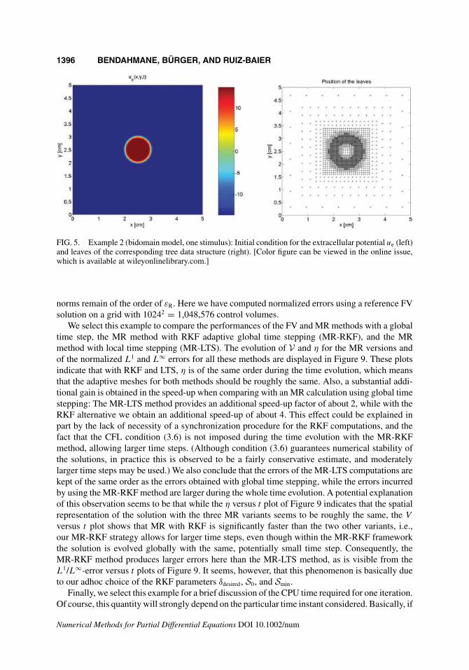
FIG. 5. Example 2 (bidomain model, one stimulus): Initial condition for the extracellular potential ue (left)and leaves of the corresponding tree data structure (right). [Color figure can be viewed in the online issue,which is available at wileyonlinelibrary.com.]

norms remain of the order of εR. Here we have computed normalized errors using a reference FVsolution on a grid with 10242 = 1,048,576 control volumes.

We select this example to compare the performances of the FV and MR methods with a globaltime step, the MR method with RKF adaptive global time stepping (MR-RKF), and the MRmethod with local time stepping (MR-LTS). The evolution of V and η for the MR versions andof the normalized L1 and L∞ errors for all these methods are displayed in Figure 9. These plotsindicate that with RKF and LTS, η is of the same order during the time evolution, which meansthat the adaptive meshes for both methods should be roughly the same. Also, a substantial addi-tional gain is obtained in the speed-up when comparing with an MR calculation using global timestepping: The MR-LTS method provides an additional speed-up factor of about 2, while with theRKF alternative we obtain an additional speed-up of about 4. This effect could be explained inpart by the lack of necessity of a synchronization procedure for the RKF computations, and thefact that the CFL condition (3.6) is not imposed during the time evolution with the MR-RKFmethod, allowing larger time steps. (Although condition (3.6) guarantees numerical stability ofthe solutions, in practice this is observed to be a fairly conservative estimate, and moderatelylarger time steps may be used.) We also conclude that the errors of the MR-LTS computations arekept of the same order as the errors obtained with global time stepping, while the errors incurredby using the MR-RKF method are larger during the whole time evolution. A potential explanationof this observation seems to be that while the η versus t plot of Figure 9 indicates that the spatialrepresentation of the solution with the three MR variants seems to be roughly the same, the V

versus t plot shows that MR with RKF is significantly faster than the two other variants, i.e.,our MR-RKF strategy allows for larger time steps, even though within the MR-RKF frameworkthe solution is evolved globally with the same, potentially small time step. Consequently, theMR-RKF method produces larger errors here than the MR-LTS method, as is visible from theL1/L∞-error versus t plots of Figure 9. It seems, however, that this phenomenon is basically dueto our adhoc choice of the RKF parameters δdesired, S0, and Smin.

Finally, we select this example for a brief discussion of the CPU time required for one iteration.Of course, this quantity will strongly depend on the particular time instant considered. Basically, if



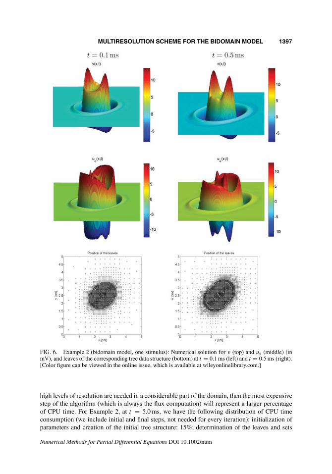
FIG. 6. Example 2 (bidomain model, one stimulus): Numerical solution for v (top) and ue (middle) (inmV), and leaves of the corresponding tree data structure (bottom) at t = 0.1 ms (left) and t = 0.5 ms (right).[Color figure can be viewed in the online issue, which is available at wileyonlinelibrary.com.]

high levels of resolution are needed in a considerable part of the domain, then the most expensivestep of the algorithm (which is always the flux computation) will represent a larger percentageof CPU time. For Example 2, at t = 5.0 ms, we have the following distribution of CPU timeconsumption (we include initial and final steps, not needed for every iteration): initialization ofparameters and creation of the initial tree structure: 15%; determination of the leaves and sets



FIG. 7. Example 2 (bidomain model, one stimulus): Numerical solution for v (top) and ue (middle) (inmV), and leaves of the corresponding tree data structure (bottom) at t = 2.0 ms (left) and t = 3.5 ms (right).[Color figure can be viewed in the online issue, which is available at wileyonlinelibrary.com.]

of virtual leaves: 10%; computation of the discretized divergence operator for all leaves: 30%;solution of a linear system (the one which is solved via Cholesky factorization): 20%; updatingthe tree structure: 15%; saving meshes, leaves and cell averages; and rest of the computations:10%. Overall, arithmetic operations related to the actual computation of the numerical solution



FIG. 8. Example 2 (bidomain model, one stimulus): Profile of the numerical solution for ue at y = 2.5(left), and leaves of the corresponding tree data structure (right) at t = 5.0 ms.

consume roughly 50% of CPU time; the remainder goes into the “overhead” of the administrationof the multiresolution representation and the graded tree.

C. Example 3

We now consider an initial stimulus at the center of �, later at t = 0.2 ms, we apply anotherinstantaneous stimulus to the northwest corner of �, and at t = 1.0 ms we apply a third stimulusof the same magnitude to the northeast and southwest corners. The system is evolved and we showsnapshots of the numerical solution for v and ue and the adaptive mesh. The numerical resultsshown in Figures 10 and 11 clearly indicate the anisotropic orientation of the fibers.

VII. CONCLUSIONS

We address the application of a MR method for FV schemes combined with LTS and RKF adap-tive time stepping for solving the bidomain equations. The numerical experiments illustrate thatthese methods are efficient and accurate enough to simulate the electrical activity in myocardialtissue with affordable effort. This is a real advantage in comparison with more involved methods

TABLE III. Example 2 (bidomain model, one stimulus): Corresponding simulated time, CPU ratio V ,compression rate η, and normalized errors.

Time t (ms) V η Potential L1−error L2−error L∞−error

0.1 13.74 19.39 v 3.68 × 10−4 8.79 × 10−5 6.51 × 10−4

ue 2.01 × 10−4 6.54 × 10−5 5.22 × 10−4

0.5 21.40 17.63 v 4.06 × 10−4 9.26 × 10−5 6.83 × 10−4

ue 2.79 × 10−4 8.72 × 10−5 5.49 × 10−4

2.0 25.23 17.74 v 4.37 × 10−4 1.25 × 10−4 6.88 × 10−4

ue 3.48 × 10−4 9.44 × 10−5 6.11 × 10−4

5.0 26.09 16.35 v 5.29 × 10−4 1.94 × 10−4 7.20 × 10−4

ue 4.15 × 10−4 1.06 × 10−4 6.32 × 10−4



FIG. 9. Example 2 (bidomain model, one stimulus): Time evolution for data compression rate η (top left),speed-up rate V (top right), and normalized L1 errors (bottom left) and L∞ errors (bottom right) for differentmethods: MR scheme with global time step, MR with locally varying time stepping and MR with RKF timestepping.

that require large scale computations on clusters. We here contribute to the recent work doneby several groups in testing whether the combination of MR, LTS, and RKF strategies is indeedeffective for a relevant class of problems.

Concerning the orders of the schemes involved, we mention that at least in the case of hyper-bolic equations, it is known that when using MR schemes of high order, and even if the referenceFV method is only of first order, the global scheme maintains the order of the MR reconstruction.In the case of the bidomain equations, we experimentally see the same behavior. This motivatesour choice of the reference tolerance in such a way that the discretization and perturbation errorsare of the same order (see Section IVD), and furthermore the order of the MR reconstruction is setto one, with r = 3 (as the order of the reference FV scheme), in Example 1. For Examples 2 and 3,we use a higher order reconstruction (of order 2, with r = 5), and this high order is inherited bythe global method. This is why we choose an RKF method of order (3)2.

From a numerical point of view, the plateau-like structures, associated with very steep gradi-ents, of typical solutions motivate the use of a locally refined adaptive mesh, since we require high



FIG. 10. Example 3 (bidomain model, three stimuli): Numerical solution for v (top) and ue (middle) (inmV), and leaves of the corresponding tree data structure (bottom) at t = 0.1 ms (left) and t = 0.5 ms (right).[Color figure can be viewed in the online issue, which is available at wileyonlinelibrary.com.]

resolution near these steep gradients only. These areas of strong variation occupy a very reducedpart of the entire domain only, especially in the case of sharp fronts. Consequently, our gain willbe less significant in the presence of chaotic electrical activity or when multiple waves interact inthe considered tissue.



FIG. 11. Example 3 (bidomain model, three stimuli): Numerical solution for transmembrane potential v(top) and extracellular potential ue (middle) (in mV), and leaves of the corresponding tree data structure(bottom) at t = 2.0 ms (left) and t = 5.0 ms (right). [Color figure can be viewed in the online issue, whichis available at wileyonlinelibrary.com.]

On the basis of our numerical examples, we conclude that using an LTS strategy, we obtain asubstantial gain in CPU time speed-up of a factor of about 2 for finer levels while the errors betweenthe MR-LTS solution and a reference solution are of the same order as those of the MR solution.On the other hand, using an MR-RKF strategy, we obtain an additional speed-up factor of about4, but at the price of larger errors. However, in assessing our findings, it is important to recognizelimitations. The high rates of compression obtained with our methods are problem-dependent and



they may depend on the proper adjustment of parameters. We have only considered here verysimple geometries, because all computations are concentrated on adaptivity and performance.Simulations on more complex and realistic geometries are part of possible future work.

Finally, we remark that the FV method given in Section III as well the MR framework detailedin Section IV are both straightforwardly extensible to the 3D case.

References

1. A. L. Hodgkin and A. F. Huxley, A quantitative description of membrane current and its application toconduction and excitation in nerve, J Physiol 117 (1952), 500–544.

2. J. Keener and J. Sneyd, Mathematical Physiology, Vols. I & II, 2nd Ed., Springer-Verlag, New York,2009.

3. L. Tung, A bi-domain model for describing ischemic myocardial D-C currents, PhD thesis, MIT,Cambridge, MA, 1978.

4. M. Bendahmane and K. H. Karlsen, Analysis of a class of degenerate reaction-diffusion systems andthe bidomain model of cardiac tissue, Netw Heterog Media 1 (2006), 185–218.

5. P. Colli Franzone, P. Deuflhard, B. Erdmann, J. Lang, and L. F. Pavarino, Adaptivity in space and timefor reaction–diffusion systems in electro-cardiology, SIAM J Sci Comput 28 (2006), 942–962.

6. P. Colli Franzone and G. Savaré, Degenerate evolution systems modeling the cardiac electric field atmicro- and macroscopic level, In: A. Lorenzi and B. Ruf, editors, Evolution equations, semigroups andfunctional analysis, Birkhäuser, Basel, 2002, pp. 49–78.

7. M. Domingues, S. Gomes, O. Roussel, and K. Schneider, An adaptive multiresolution scheme with localtime-stepping for evolutionary PDEs, J Comput Phys 227 (2008), 3758–3780.

8. A. Cohen, S. Kaber, S. Müller, and M. Postel, Fully adaptive multiresolution finite volume schemes forconservation laws, Math Comp 72 (2001), 183–225.

9. O. Roussel, K. Schneider, A. Tsigulin, and H. Bockhorn, A conservative fully adaptive multiresolutionalgorithm for parabolic PDEs, J Comput Phys 188 (2003), 493–523.

10. M. Bendahmane, R. Bürger, R. Ruiz-Baier, and K. Schneider, Adaptive multiresolution schemes withlocal time stepping for two-dimensional degenerate reaction-diffusion systems, Appl Numer Math 59(2009), 1668–1692.

11. R. Bürger, R. Ruiz, K. Schneider, and M. Sepúlveda, Fully adaptive multiresolution schemes for stronglydegenerate parabolic equations in one space dimension, M2AN Math Model Numer Anal 42 (2008),535–563.

12. R. Bürger, R. Ruiz, K. Schneider, and M. Sepúlveda, Fully adaptive multiresolution schemes for stronglydegenerate parabolic equations with discontinuous flux, J Engrg Math 60 (2008), 365–385.

13. E. Cherry, H. Greenside, and C. S. Henriquez, Efficient simulation of three–dimensional anisotropiccardiac tissue using an adaptive mesh refinement method, Chaos 13 (2003), 853–865.

14. H. Chen and X.-H. Zhong, Global existence and blow-up for the solutions to nonlinear parabolic/ellipticsystem modelling chemotaxis, IMA J Appl Math 70 (2005), 221–240.

15. Y. Bourgault, Y. Coudière, and C. Pierre, Existence and uniqueness of the solution for the bidomainmodel used in cardiac electro-physiology, Nonlin Anal Real World Appl 10 (2009), 458–482.

16. W. Quan, S. Evans, and H. Hastings, Efficient integration of a realistic two-dimensional cardiac tissuemodel by domain decomposition, IEEE Trans Biomed Eng 45 (1998), 372–385.

17. J. Sundnes, G. T. Lines, and A. Tveito, An operator splitting method for solving the bidomain equationscoupled to a volume conductor model for the torso, Math Biosci 194 (2005), 233–248.

18. K. Skouibine, N. Trayanova, and P. Moore, A numerically efficient model for simulation of defibrillationin an active bidomain sheet of myocardium, Math Biosci 166 (2000), 85–100.



19. M. J. Berger and J. Oliger, Adaptive mesh refinement for hyperbolic partial differential equations, JComput Phys 53 (1984), 482–512.

20. P. Colli Franzone and L. F. Pavarino, A parallel solver for reaction-diffusion systems in computationalelectro-cardiology, Math Models Meth Appl Sci 14 (2004), 883–911.

21. H. Saleheen and K. Ng, A new three–dimensional finite-difference bidomain formulation for inhomo-geneous anisotropic cardiac tissues, IEEE Trans Biomed Eng 45 (1998), 15–25.

22. A. Harten, Multiresolution algorithms for the numerical solution of hyperbolic conservation laws, CommPure Appl Math 48 (1995), 1305–1342.

23. S. Müller, Adaptive Multiscale Schemes for Conservation Laws, Springer-Verlag, Berlin, 2003.

24. G. Chiavassa, R. Donat, and S. Müller, Multiresolution-based adaptive schemes for hyperbolic conser-vation, in: T. Plewa, T Linde, V. G. Weiss (Editors), Adaptive mesh refinement-theory and applications,Springer-Verlag, Berlin, 2003, pp. 137–159.

25. W. Dahmen, B. Gottschlich-Müller, and S. Müller, Multiresolution schemes for conservation laws,Numer Math 88 (2001), 399–443.

26. S. Müller and Y. Stiriba, Fully adaptive multiscale schemes for conservation laws employing locallyvarying time stepping, J Sci Comput 30 (2007), 493–531.

27. J. Sundnes, G. T. Lines, X. Cai, B. F. Nielsen, K.-A. Mardal, and A. Tveito, Computing the electricalactivity in the heart, Springer-Verlag, Berlin, 2006.

28. C. Mitchell and D. Schaeffer, A two-current model for the dynamics of cardiac membrane, Bull MathBiol 65 (2001), 767–793.

29. P. Colli Franzone, L. F. Pavarino, and B. Taccardi, Simulating patterns of excitation, repolarization andaction potential duration with cardiac bidomain and monodomain models, Math Biosci 197 (2005),35–66.

30. P. R. Johnston, The effect of simplifying assumptions in the bidomain model of cardiac tissue:Application to ST segment shifts during partial ischaemia, Math Biosci 198 (2005), 97–118.

31. M. Bendahmane and K. H. Karlsen, Convergence of a finite volume scheme for the bidomain model ofcardiac tissue, Appl Numer Math 59 (2009), 2266–2284.

32. Y. Coudière, C. Pierre, and R. Turpault, Solving the fully coupled heart and torso problems of elec-tro cardiology with a 3D discrete duality finite volume method. HAL preprint (2006), available fromhttp://hal.archives-ouvertes.fr/ccsd-00016825.

33. M. Bendahmane, R. Bürger, and R. Ruiz-Baier, A finite volume scheme for cardiao propagation inmedia with isotropic conductivites. Preprint, Universidad de Concepción; submitted.

34. M. Pennacchio and V. Simoncini, Efficient algebraic solution of reaction-diffusion systems for thecardiac excitation process, J Comput Appl Math 145 (2002), 49–70.

35. P. K. Moore, An adaptive finite element method for parabolic differential systems: some algorithmicconsiderations in solving in three space dimensions, SIAM J Sci Comput 21 (2000), 1567–1586.


a multiresolution space-time adaptive scheme for the...

Documents