multiresolution isosurface extraction with adaptive ...ttwong/papers/asc/asc.pdf · multiresolution...

EUROGRAPHICS ’98 / N. Ferreira and M. G¨obel(Guest Editors)

Volume 17, (1998), Number 3

Multiresolution Isosurface Extraction withAdaptive Skeleton Climbing

Tim Postony Tien-Tsin Wongz Pheng-Ann Hengz

[email protected] [email protected] [email protected]

yCenter for Information-Enhanced Medicine, National University of SingaporezDept. of Computer Science & Eng., The Chinese University of Hong Kong

Abstract

An isosurface extraction algorithm which can directly generate multiresolution isosurfaces from volume data is in-troduced. It generates low resolution isosurfaces, with 4 to 25 times fewer triangles than that generated by march-ing cubes algorithm, in comparable running times. By climbing from vertices (0-skeleton) to edges (1-skeleton) tofaces (2-skeleton), the algorithm constructs boxes which adapt to the geometry of the true isosurface. Unlike pre-vious adaptive marching cubes algorithms, the algorithm does not suffer from the gap-filling problem. Althoughthe triangles in the meshes may not be optimally reduced, it is much faster than postprocessing triangle reductionalgorithms. Hence the coarse meshes it produces can be used as the initial starts for the mesh optimization, ifmesh optimality is the main concern.

1. Introduction

Standard isosurface extraction algorithms1 generate an un-wieldy number of triangles (half a million is common for abrain surface), making graphics and interactions unwieldy.This is inevitable with approaches which create triangles ly-ing within voxel-sized cubes, even where a surface is smoothenough to be well approximated by much larger facets. Meshreduction algorithms2; 3; 4; 5 can greatly reduce the trianglecount and preserve the geometrical details of the isosurfaces.Unfortunately, these postprocessing algorithms are usuallytime consuming. Hence they are only good for creating eco-nomical surfaces for later use. They are less useful when fastcreation and display of isosurfaces are required, and whenthe exact threshold value is not certain. For instance, a sur-geon may have to try different threshold values to explore thetumor surfaces. Rapid creation of accurate, economical iso-surfaces is vital to many forms of volume data exploration,from neurosurgery to the planning of a gold mine.

We describe here a direct construction of isosurfaces withbetween 4 and 25 times fewer triangles than marching cubesalgorithms1; 6 (depending on the complexity of the volume),in comparable running times. Hence more complexity canbe handled at interactive speed. The proposed algorithm is

named asadaptive skeleton climbing. Since we constructthe isosurfaces by first finding iso-points on grid edges (1-skeleton), then iso-lines on faces (2-skeleton) and finally iso-surfaces within boxes (3-skeleton), this approach is known intopology asskeleton climbing. Moreover, the size of the con-structed boxes will adapt to the geometry of the isosurface(e.g.larger boxes for smoother regions), hence it isadaptive.

Our approach is quite different from the previous adap-tive marching cubes algorithms7; 8. We do not need a crack-patching step because we build compatibility (describedshortly) into the faces where cells meet before generatingtriangles.

The proposed algorithm generates isosurfaces in multipleresolutions directly. The coarseness of the generated meshesis controlled by a single parameter. The triangle reductionis done on the fly as the isosurfaces are generated withoutgoing through a separate postprocess. The proposed on-the-fly triangle reduction approach can generate more accuratemeshes because it directly make use of the voxel values inthe volume. On the other hand, the postprocessing trianglereduction approaches2; 3; 4; 5 usually use the indirect geo-metrical information from the approximated meshes.

The algorithm also exhibits a nice feature that coarser iso-

c The Eurographics Association and Blackwell Publishers 1998. Published by BlackwellPublishers, 108 Cowley Road, Oxford OX4 1JF, UK and 350 Main Street, Malden, MA02148, USA.

http://www.cse.cuhk.edu.hk/~ttwong/

http://beast.cbmv.jhu.edu:8000/people/tim/

http://www.cse.cuhk.edu.hk/~pheng/

http://www.cse.cuhk.edu.hk/~ttwong/papers/asc/asc.html

Poston, Wong and Heng / Multiresolution Isosurface Extraction with Adaptive Skeleton Climbing

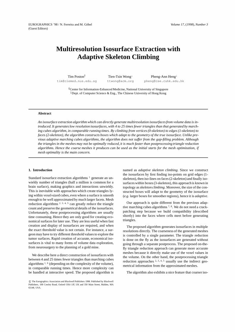
Figure 1: Overview of adaptive skeleton climbing.

surfaces require smaller amount of time to generate. This isopposed to the case of mesh optimization approach3 whichrequires longer time to generate coarser meshes. Hence ourmethod allows the user to first generate a low resolutionmesh as a preview before deciding to generate the detailedhigh resolution mesh.

1.1. Overview

The algorithm can be intuitively subdivided into four steps:

1. Volume analysis.2. Construction of simple boxes.3. Sharing information between adjacent boxes.4. Isosurface extraction.

In order to fit large triangles to smooth regions, the con-tent inside the volume must be first analysed. The volumeis implicitly analysed through the manipulation of basic 1Dand 2D data structures in step 1. In step 2, the data structuresbuilt allow us to construct the 3Dsimpleboxes (describedin section 3) whose sizes are closely related to the geometrycomplexity of the enclosed isosurface. Information is thenshared between adjacent boxes to prevent existence of gapin step 3. And finally in step 4, the triangular mesh is gen-erated. Figure 1 shows the processes of adaptive skeletonclimbing graphically. The basic idea is to group voxels firstin 1D (segments), then in 2D (rectangles) and finally in 3D(boxes).

Section 2 describes the step of implicit volume analysis indetail. Section 3 discusses the construction of simple boxes.Information sharing step is described in section 4. Some de-tails of triangular mesh generation are discussed in section 5.Section 6 discusses how the algorithm is used to generatemultiresolution isosurfaces on the fly. Section 7 discusses

the practical implementation, shows the results and com-pares them with marching cubes. Finally, section 8 gives ourconclusions and future directions.

2. Volume Analysis

The first step of the algorithm is to analyse the volumethrough manipulating the basic 1D and 2D data structures.We start the analysis in 1D,i.e. consider a linear sequenceof voxel samples. Try to find out the length-maximal subse-quences of voxels withsimplestructure (described shortly).Then we go on to the 2D data structure and find out the size-maximal rectangular regions of voxel samples withsimplestructure.

2.1. 1D Data Structures and Manipulation

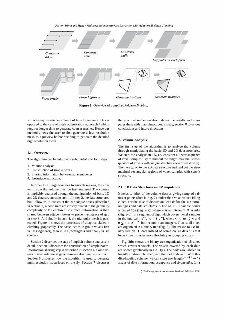
It helps to think of the volume data as giving sampled val-ues at points (dots in Fig. 2), rather than voxel values fillingcubes. For the sake of discussion, let’s define the 1D termi-nologies and data structures. A line of2n+1 sample pointsis calledlign (Fig. 2(a)) wheren is an integer� 0. A dike(Fig. 2(b)) is a segment of lign which covers voxel samplesin the interval[a2m; (a + 1)2m], where0 � m � n and0 � a < 2n�m, botha andm are integers. That is, all dikesare organized in a binary tree (Fig. 3). The reason to use bi-nary tree on 1D data instead of octree on 3D data8 is thatbinary tree provides more flexibility in grouping voxels.

Fig. 3(b) shows the binary tree organization of 15 dikeswhich covers 9 voxels. The voxels covered by each dikeare shown graphically in Fig. 3(c). The nodes are labeled inbreadth-first-search order, with the root node as 1. With thisdike-labeling scheme, we can store two length-(2n+1 � 1)

arrays of dike information,occupancyandsimple dike, for a

c The Eurographics Association and Blackwell Publishers 1998.


Figure 2: Basic 1D data structures.

lign of 2n + 1 samples. For simplicity, letN = 2n for shorthand.

Figure 3: Binary tree organization of 1D voxel data.

Theoccupancy arrayof a lign describes the presence ofiso-points (1D analogy of 3D isosurface) on its dikes. Withthis occupancy array, we can accurately locate the positionof iso-point and how the isosurface crosses the lign. Now,let us denote the voxel sample with value above or equal tothe threshold (� ) as�, and sample with value below� as�.Then the binary value of theith entry in the occupancy arraymeans:

occ[ i] =

(002 all samples in dikei are on the same side of� .012 if dike i is crossed by isosurface once, upward� ! �:

102 if dike i is crossed by isosurface once, downward� ! �:

112 if dike i is crossed by isosurface more than once.

Note the binary values symbolize the crossing conditions.For instance, if the isosurface crosses the dike once and thevoxels within the dike change from� (0) on the left to�(1) on the right, then the value inocc[] is 012 (� ! �).Once the entries of unit dikes (leaf nodes of the binary tree)are initialized directly from volume data, the entries of thenon-unit dikes (upper interior nodes) can be found by apply-ing a recursive bitwise OR operations on the leaf nodes. Thevalues inocc[] are specially designed.

occ[ i] := (occ[ 2i]) OR (occ[ 2i + 1])

Another array issimple dike array. It tells us the length-maximalsimpledikes inside the lign. A dikei is simpleifocc [i] < 112 ; that is, the dike is crossed at most once bythe isosurface. The entrysimple[ i] holds the index of thelength-maximal simple dike with the same left end as dikei.

Intuitively speaking, simple dike array tells us which vox-els can be grouped together without violating the binaryboundary due to the tree organization (binary edgefor short)and the simplicity constraints. The length-maximal simplestep following dikei is the dikesimple[ i+1] . By per-forming the following pseudocode fragment, we can walk

through the lign in steps of length-maximal dikes in an effi-cient way.

current := simple[1]while current 6= ”end of walk” mark

current := simple[current+1]

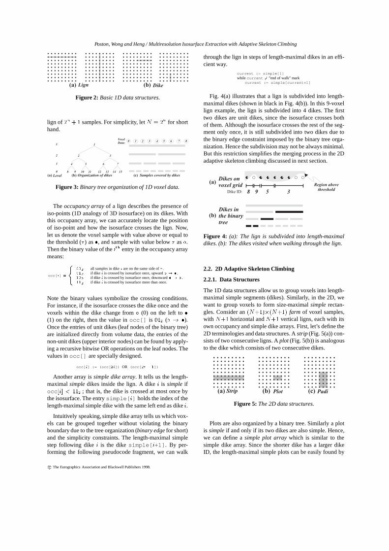
Fig. 4(a) illustrates that a lign is subdivided into length-maximal dikes (shown in black in Fig. 4(b)). In this 9-voxellign example, the lign is subdivided into 4 dikes. The firsttwo dikes are unit dikes, since the isosurface crosses bothof them. Although the isosurface crosses the rest of the seg-ment only once, it is still subdivided into two dikes due tothe binary edge constraint imposed by the binary tree orga-nization. Hence the subdivision may not be always minimal.But this restriction simplifies the merging process in the 2Dadaptive skeleton climbing discussed in next section.

Figure 4: (a): The lign is subdivided into length-maximaldikes. (b): The dikes visited when walking through the lign.

2.2. 2D Adaptive Skeleton Climbing

2.2.1. Data Structures

The 1D data structures allow us to group voxels into length-maximal simple segments (dikes). Similarly, in the 2D, wewant to group voxels to form size-maximalsimplerectan-gles. Consider an(N+1)�(N+1) farm of voxel samples,with N+1 horizontal andN+1 vertical ligns, each with itsown occupancy and simple dike arrays. First, let’s define the2D terminologies and data structures. Astrip (Fig. 5(a)) con-sists of two consecutive ligns. Aplot (Fig. 5(b)) is analogousto the dike which consists of two consecutive dikes.

Figure 5: The 2D data structures.

Plots are also organized by a binary tree. Similarly a plotis simpleif and only if its two dikes are also simple. Hence,we can define asimple plot arraywhich is similar to thesimple dike array. Since the shorter dike has a larger dikeID, the length-maximal simple plots can be easily found by



performing aMAXoperation on each pair of elements in thesimple dike arrays of the two consecutive ligns.

strip[ j].simple[ i] := MAX(lign[ j].simple[ i],lign[ j + 1].simple[ i])

Fig. 6 shows one such operation graphically. The calcu-lated plots are overlaid with the voxel samples in Fig. 6(b).Note that each plot is crossed at most twice by the isosurface.

Figure 6: Length-maximal plots from consecutive ligns.

2.2.2. Merging Plots to Form Padis

A rectangle with dikes as sides is calledpadi (Fig. 5(c)). Apadi is simple if all plots inside it and its four side dikesare simple. Our goal is to subdivide the 2D farm of voxelsinto size-maximal padis. To do so, neighboring simple plotsare merged to form simple padis (Fig. 7), as large as possi-ble. Note there is no unique way to merge plots. Differentmerging strategy gives different sets of padis. Fig. 7 showstwo alternatives when merging the two consecutive strips.Even an optimal merging is found for 2D, it may not yieldan optimal merging in 3D (discussed in next section). More-over, a fast algorithm is crucially required since it will befrequently executed. A slow optimistic algorithm is uselessin this case. Hence we do not use any optimistic algorithm tosearch for the optimal merging. A heuristic bottom-up merg-ing (ASC2D, Fig. 8) is used due to its efficiency and simplic-ity.

Figure 7: Merging plots to form padis.

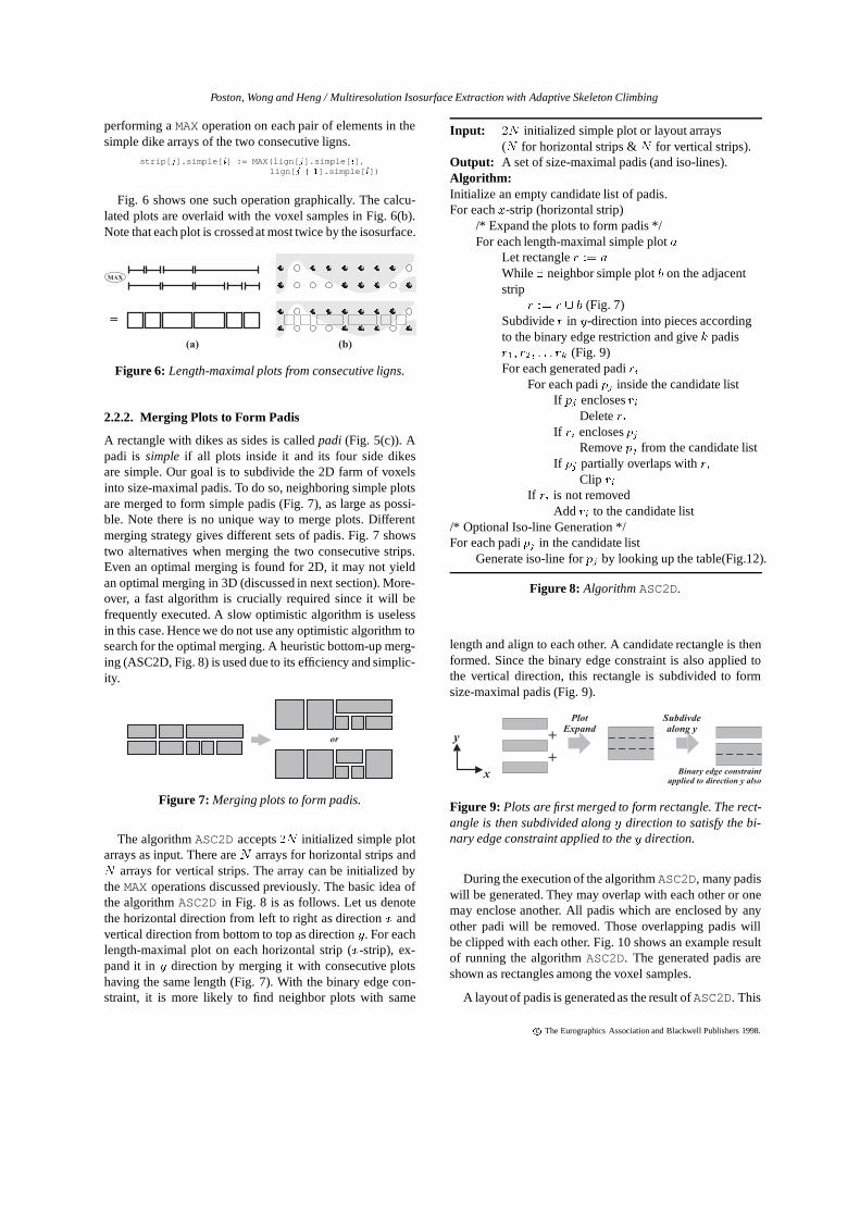
The algorithmASC2Daccepts2N initialized simple plotarrays as input. There areN arrays for horizontal strips andN arrays for vertical strips. The array can be initialized bytheMAXoperations discussed previously. The basic idea ofthe algorithmASC2Din Fig. 8 is as follows. Let us denotethe horizontal direction from left to right as directionx andvertical direction from bottom to top as directiony. For eachlength-maximal plot on each horizontal strip (x-strip), ex-pand it iny direction by merging it with consecutive plotshaving the same length (Fig. 7). With the binary edge con-straint, it is more likely to find neighbor plots with same

Input: 2N initialized simple plot or layout arrays(N for horizontal strips &N for vertical strips).

Output: A set of size-maximal padis (and iso-lines).Algorithm:Initialize an empty candidate list of padis.For eachx-strip (horizontal strip)

/* Expand the plots to form padis */For each length-maximal simple plota

Let rectangler := a

While 9 neighbor simple plotb on the adjacentstrip

r := r [ b (Fig. 7)Subdivider in y-direction into pieces accordingto the binary edge restriction and givek padisr1; r2; : : : rk (Fig. 9)For each generated padiri

For each padipj inside the candidate listIf pj enclosesri

DeleteriIf ri enclosespj

Removepj from the candidate listIf pj partially overlaps withri

Clip riIf ri is not removed

Add ri to the candidate list/* Optional Iso-line Generation */For each padipj in the candidate list

Generate iso-line forpj by looking up the table(Fig.12).

Figure 8: AlgorithmASC2D.

length and align to each other. A candidate rectangle is thenformed. Since the binary edge constraint is also applied tothe vertical direction, this rectangle is subdivided to formsize-maximal padis (Fig. 9).

Figure 9: Plots are first merged to form rectangle. The rect-angle is then subdivided alongy direction to satisfy the bi-nary edge constraint applied to they direction.

During the execution of the algorithmASC2D, many padiswill be generated. They may overlap with each other or onemay enclose another. All padis which are enclosed by anyother padi will be removed. Those overlapping padis willbe clipped with each other. Fig. 10 shows an example resultof running the algorithmASC2D. The generated padis areshown as rectangles among the voxel samples.

A layout of padis is generated as the result ofASC2D. This



Figure 10: Example result of running algorithmASC2D.

Figure 11: Storing the padi layout in layout arrays.

layout information is stored implicitly in the layout arrays.Layout array is very similar to the simple plot array but withthe constraint that no plot may cross the boundary of anygenerated padi on the layout. For a farm of(N +1)� (N +

1) voxels,2N layout arrays are defined,N x-strips andNy-strips. Theith entry in x-strip (y-strip) stores the indexof the length-maximal plot that fits into the padi layout andshares its left (bottom) end with ploti. Fig. 11 shows the padilayout of a5 � 5 xy-farm, which is represented byx-strips(Fig. 11(b)) andy-strips (Fig. 11(c)). The reason to store thelayout in this way is to simplify the simple box constructiondiscussed in section 3.

2.2.3. Iso-line Generation

Once the size-maximal padis are found, we can generate 2Diso-lines which separate� voxels from those� voxels. Al-though we will not generate any iso-lines until the 3D boxeshave been constructed (discussed in next section). For thesake of presentation, it is more convenient to discuss it here.

The iso-line can be efficiently generated by looking upa 2D padi configuration table in Fig. 12, instead of a 3Dvoxel cube configuration table as in marching cubes algo-rithms 1; 6. Fig. 12 shows all possible padi configurationsand their corresponding iso-lines. Note the padi needs notbe a square. Similar to the 3D voxel configurations, ambigu-

Figure 12: Generate iso-lines by a 16-entry table. Two am-biguous cases lead to subsampling.

ity also exists on 2D padi configurations (the two lower leftconfigurations in Fig. 12).

The ambiguity with two diagonally opposite� cornerscan sometimes be resolved by subsampling at the center ofthe padi. However, wrong iso-lines will still be generated insome cases (Fig. 13). Where connectivity is crucial, softwareshould warn the user of ambiguous cases and offer finer,more CPU-costly tools for local investigation. In many casesthe warning is as useful to the surgeon, geologist or otheruser as any silently-attempted best guess by the software.

Figure 13: Bad ambiguity resolution by subsampling.

The generated padis (shown as rectangles) and iso-lines(shown as thick lines) are overlaid on the 2D voxel grid inFig. 10. The algorithm isolates� from � voxels, with 30edges on 23 adaptive padis rather than the 46 edges on 64unit squares. The feature is the key how the algorithm re-duces triangles.

3. Construction of Simple Boxes

By manipulating these 1D and 2D data structures, enoughinformation is provided for us to construct 3Dsimpleboxes.The information is implicitly stored as the 2D padis. Us-ing this information, we go on to construct simple boxes bystacking simple padis.



3.1. 3D Adaptive Skeleton Climbing

3.1.1. 3D Data Structures

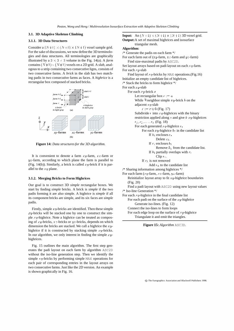
Consider a(N+1) � (N+1)� (N+1) voxel sample grid.For the sake of discussions, we now define the 3D terminolo-gies and data structures. All terminologies are graphicallyillustrated by a3 � 3� 3 volume in the Fig. 14(a). Afarmcontains(N+1)�(N+1) voxels on a 2D grid. Aslab, anal-ogous to a strip containing two consecutive ligns, consists oftwo consecutive farms. Abrick in the slab has two match-ing padis in two consecutive farms as faces. Ahighrice is arectangular box composed of stacked bricks.

Figure 14: Data structures for the 3D algorithm.

It is convenient to denote a farmxy-farm, xz-farm oryz-farm, according to which plane the farm is parallel to(Fig. 14(b)). Similarly, a brick is calledxy-brick if it is par-allel to thexy plane.

3.1.2. Merging Bricks to Form Highrices

Our goal is to construct 3Dsimple rectangular boxes. Westart by findingsimplebricks. A brick issimpleif the twopadis forming it are also simple. A highrice issimpleif allits component bricks are simple, and its six faces aresimplepadis.

Firstly, simplexy-bricks are identified. Then these simplexy-bricks will be stacked one by one to construct the sim-ple xy-highrice. Note a highrice can be treated as compos-ing of xy-bricks,xz-bricks oryz-bricks, depends on whichdimension the bricks are stacked. We call a highrice thexy-highrice if it is constructed by stacking simplexy-bricks.In our algorithm, we only interest in finding the simplexy-highrices.

Fig. 15 outlines the main algorithm. The first step gen-erates the padi layout on each farm by algorithmASC2Dwithout the iso-line generation step. Then we identify thesimplexy-bricks by performing simpleMAXoperations foreach pair of corresponding entries in the layout arrays ontwo consecutive farms. Just like the 2D version. An exampleis shown graphically in Fig. 16.

Input: An (N+1)� (N+1)� (N+1) 3D voxel grid.Output: A set of maximal highrices and isosurface

triangular mesh.Algorithm:/* Generate the padis on each farm */For each farm out of (xy-farm,xz-farm andyz-farm)

Find size-maximal padis byASC2D.Set layout arrays based on padi layout on eachxy-farm.For eachxy-slab

Find layout ofxy-bricks byMAXoperations.(Fig.16)Initialize an empty candidate list of highrices./* Stack the bricks to form highrice */For eachxy-slab

For eachxy-brick aLet rectangular boxr := a

While 9 neighbor simplexy-brick b on theadjacentxy-slab

r := r [ b (Fig. 17)Subdivider into xy-highrices with the binaryrestriction applied alongz and givek xy-highricesr1; r2; : : : ; rk (Fig. 18)For each generatedxy-highricerk

For eachxy-highricehl in the candidate listIf hl enclosesrk

Deleterk.If ri encloseshl

Removehj from the candidate list.If hl partially overlaps withri

Clip rl.If rk is not removed

Add rk to the candidate list/* Sharing information among highrices */For each farm (xy-farm,xz-farm,yz-farm)

Reinitialize layout array to fitxy-highrice boundaries(Fig. 20)Find a padi layout withASC2Dusing new layout values

/* Iso-line Generation */For eachxy-highrice in the final candidate list

For each padi on the surface of thexy-highriceGenerate iso-lines. (Fig. 12)

Connect the iso-lines to form loopsFor each edge loop on the surface ofxy-highrice

Triangulate it and emit the triangles.

Figure 15: AlgorithmASC3D.



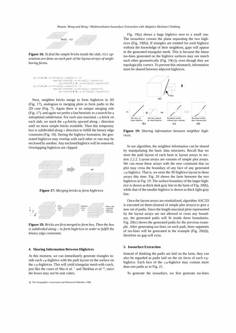
Figure 16: To find the simple bricks inside the slab,MAXop-erations are done on each pair of the layout arrays of neigh-boring farms.

xy-slab[ k].x-strip[ j].layout[ i] :=max(xy-farm[ k].x-strip[ j].layout[ i],

xy-farm[ k + 1].x-strip[ j].layout[ i])xy-slab[ k].y-strip[ j].layout[ i] :=

max(xy-farm[ k].y-strip[ j].layout[ i],xy-farm[ k + 1].y-strip[ j].layout[ i])

Next, neighbor bricks merge to form highrices in 3D(Fig. 17), analogous to merging plots to form padis in the2D case (Fig. 7). Again there is no unique merging rule(Fig. 17), and again we prefer a fast heuristic to a search for asuboptimal subdivision. For each size-maximalxy-brick oneach slab, we stack thexy-bricks upward alongz directionuntil no more simple bricks available. Then this temporarybox is subdivided alongz direction to fulfill the binary edgeconstraint (Fig. 18). During the highrice formation, the gen-erated highrices may overlap with each other or one may beenclosed by another. Any enclosed highrice will be removed.Overlapping highrices are clipped.

Figure 17: Merging bricks to form highrices

Figure 18: Bricks are first merged to form box. Then the boxis subdivided alongz to form highrices in order to fulfill thebinary edge constraint.

4. Sharing Information Between Highrices

At this moment, we can immediately generate triangles in-side eachxy-highrice with the padi layout on the surface onthexy-highrices. This will yield triangular mesh with crack,just like the cases of Shuet al. 7 and Shekharet al. 8, sincethe boxes may not be unit cubes.

Fig. 19(a) shows a large highrice next to a small one.The isosurface crosses the plane separating the two high-rices (Fig. 19(b)). If triangles are emitted foreach highricewithout the knowledge of their neighbors, gaps will appearin the generated triangular mesh. This is because the lineariso-lines generated on the highrice surfaces may not matcheach other geometrically (Fig. 19(c)), even though they aretopologically correct. To prevent this mismatch, informationmust be shared between adjacent highrices.

Figure 19: Sharing information between neighbor high-rices.

In our algorithm, the neighbor information can be sharedby manipulating the basic data structures. Recall that westore the padi layout of each farm in layout arrays in sec-tion 2.2.2. Layout arrays are variants of simple plot arrays.We can reuse these arrays with the new constraint that noplot may cross the boundary of any face of any generatedxy-highrice. That is, we store the 3D highrice layout in thesearrays this time. Fig. 20 shows the farm between the twohighrices in Fig. 19. The surface boundary of the larger high-rice is shown as thick dark gray line in the farm of Fig. 20(b),while that of the smaller highrice is shown as thick light grayline.

Once the layout arrays are reinitialized, algorithm ASC2Dis executed on them (instead of simple plot arrays) to give anew set of padis. Since the length-maximal plots representedby the layout arrays are not allowed to cross any bound-ary, the generated padis will fit inside these boundaries.Fig. 20(c) shows the generated padis for the previous exam-ple. After generating iso-lines on each padi, three segmentsof iso-lines will be generated in the example (Fig. 20(d)),therefore no gap will exist.

5. Isosurface Extraction

Instead of thinking the padis are laid on the farm, they canalso be regarded as padis laid on the six faces of eachxy-highrice. Each face of thexy-highrice may contain morethan one padis as in Fig. 21.

To generate the isosurface, we first generate iso-lines



Figure 20:Once we reinitialize the layout arrays to store the3D highrices’ layout,ASC2Dcan be run to generate padisthat fit into the surface boundaries of both highrices.

Figure 21: The six faces of a highrice are tiled withpadisafter information sharing.

on padis by looking up the 2D padi configuration tablein Fig. 12, and connect them to form closed edge loops(Fig. 23(a)). Note that in our algorithm, we only need a 2Dpadi configuration table, no 3D voxel cube configuration ta-ble is needed.

Given an edge loop consisting of several verticesvi, weemit triangles as follows. In each iteration, three consecutiveverticesvi, vi+1 andvi+2 are selected and one triangle isgenerated (Fig. 22). The vertexvi+1 is then removed fromthe edge loop. The algorithm continues until only two ver-tices are left.

Figure 22: In each iteration, one triangle is emitted and onevertex is removed.

An edge loop can be triangulated in multiple ways. Differ-ent sequences give triangular meshes with identical triangle

counts, but with different geometry (Fig. 23(b) and (c)). Togenerate a mesh that closely approximates the true isosur-face, we make use of the gradient. We reject any trianglewith planar normal vector~nt that largely deviates from thegradients~gi at three vertices. The deviation is measured bythe dot product of~nt and~gi. A threshold is used as a criteria.The threshold constraint will be relaxed if no triangle can begenerated under current constraint.

Figure 23: Triangulate the edge loop to emit triangles.

6. Multiresolution Isosurface Extraction

The proposed algorithm handles volume with the size of(N +1)� (N +1)� (N +1), i.e a cubicblock. To handlevolume with different size, we can simply tile the blocks tocover the whole volume and applyASC3Dto each block. Re-call that gaps will appear if no information is shared betweenadjacent highrices. Similarly, cracks will appear if informa-tion is not shared between adjacent blocks. Unlike the caseof variable-sized highrices, each block has the same size.This simplifies the process. To share information betweenblocks, we simply performMAXoperations on each pair oflayout arrays on the surfaces (which are also farms) of twoadjacent blocks. The simpleMAXoperations effectively findout the largest padis that fit the constraints. This informa-tion sharing process must be done just after the informationsharing among highrices.

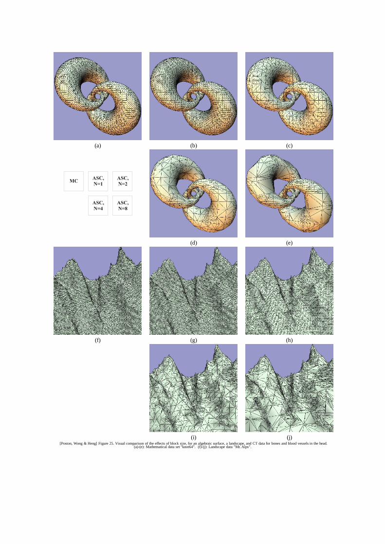
Up to this moment, we have not yet discussed the effectof using different values ofN , i.e. the size of the block.The block size constrains the maximum size of the high-rices. When the block size is small, sayN = 1, the largesthighrice contains2 � 2 � 2 voxels, i.e. same as standardmarching cubes. When a larger block size is used, largerhighrices are allowed to be generated, hence larger triangles.In other words, by controlling the valueN , we can gener-ate isosurfaces in multiresolution. Note that parameterN isan indirect control, the actual mesh generated will also de-pend on the geometry of the true isosurface. More triangleswill still be generated if the isosurface geometry is complex.Figure 25(b)-(e) shows the results of using different blocksizes. From (b) to (e), the values ofN are 1, 2, 4 and 8.As the block size increases, larger triangles are generated toapproximate the smooth surface.

Unlike the triangle reduction algorithms2; 3; 4; 5 whichgenerate coarser mesh based on the high resolution mesh, theproposed approach generates coarser mesh directly from the



original volume data. This ensures no distortion or error isintroduced before the triangle reduction. More importantly,the proposed algorithm is a on-the-fly process which re-quires no time-consuming postprocessingtriangle reduction.In fact, the algorithm produces coarser mesh in a smalleramount of time (see Table 1). This is quite different fromthose triangle reduction algorithms. Although our approachmay not reduce triangles as much as mesh optimizer does, itis a cost effective method to significantly reduce triangles ina short period of time.

7. Implementation and Results

In practical implementation, there is no need to process ev-ery block of voxels. Since many blocks are empty,i.e. con-tains no isosurface, we can simply ignore them without per-forming the computation intensive merging processes. Thiscan be done in the early stage of the algorithm. Once we haveinitialized the values inocc[] for each lign in the block, theemptiness of the block can be immediately identified.

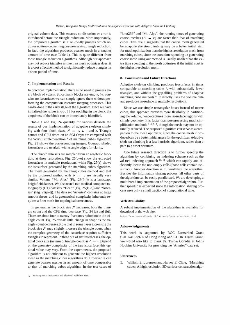
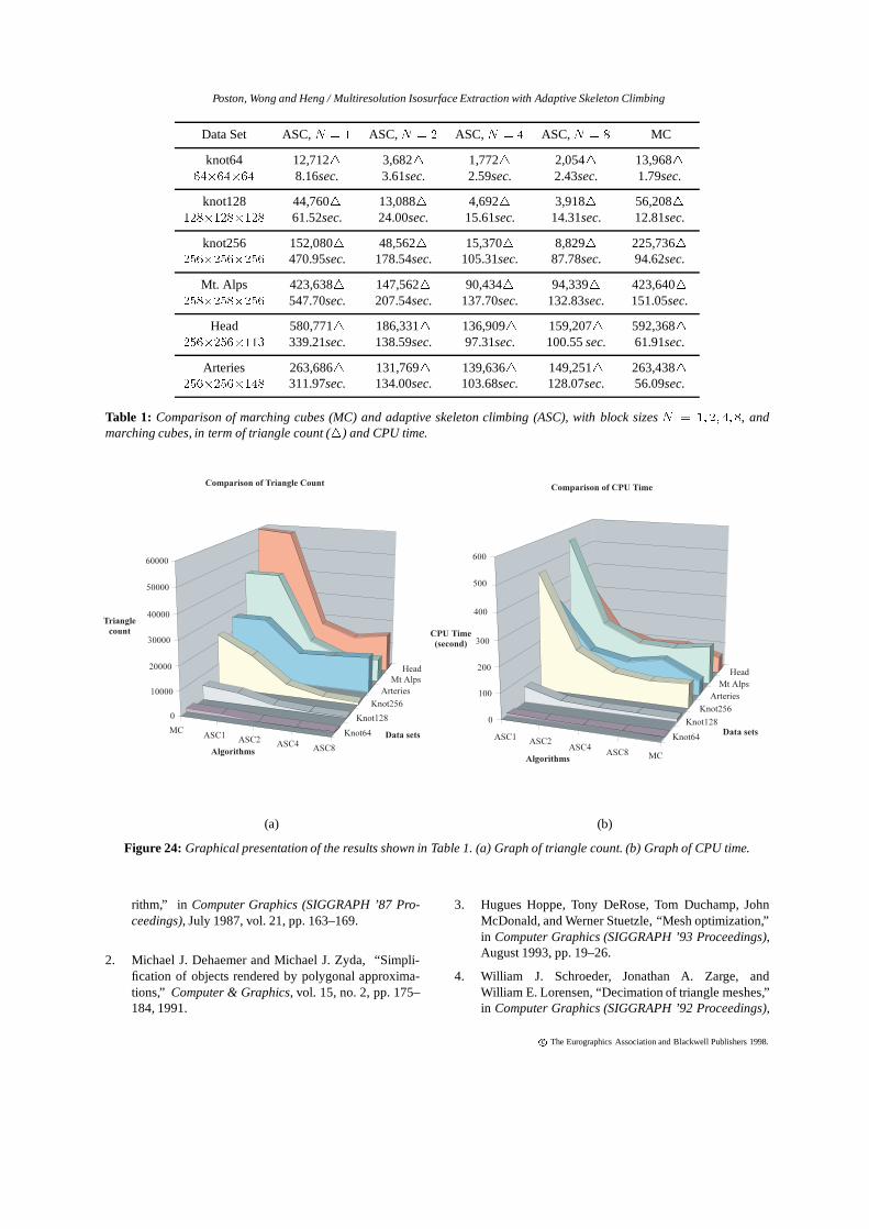
Table 1 and Fig. 24 quantify for various datasets theresults of our implementation of adaptive skeleton climb-ing with four block sizes,N = 1, 2, 4 and 8. Trianglecounts and CPU times on an SGI Onyx are compared withthe Wyvill implementation6 of marching cubes algorithm.Fig. 25 shows the corresponding images. Gouraud shadedisosurfaces are overlaid with triangle edges for clarity.

The “knot” data sets are sampled from an algebraic func-tion, at three resolutions. Fig. 25(b–e) show the extractedisosurfaces in multiple resolutions, while Fig. 25(a) showsthe isosurface generated by the marching cubes algorithm.The mesh generated by marching cubes method and thatby the proposed method withN = 1 are visually verysimilar. Volume “Mt. Alps” (Fig. 25(f–j)) is a landscapeheightfield dataset. We also tested two medical computed to-mography (CT) datasets, “Head” (Fig. 25(k–o)) and “Arter-ies” (Fig. 25(p–t)). The data set “Arteries” contains no largesmooth sheets, and its geometrical complexity inherently re-quires a finer mesh for topological correctness.

In general, as the block sizeN increases, both the trian-gle count and the CPU time decrease (Fig. 24 (a) and (b)).There are about four to twenty-five times reduction in the tri-angle count. Fig. 25 revealslittle change in shape as the tri-angle count decreases.Note that in some cases increasing theblock sizeN may slightly increase the triangle count whenthe complex geometry of the isosurface requires sufficienttriangles to represent. In three out of six tested cases, the op-timal block size (in term of triangle count) isN = 4. Dependon the geometry complexity of the true isosurface, this op-timal value may vary. From the experiments, the proposedalgorithm is not efficient to generate the highest-resolutionmesh as the marching cubes algorithms do. However, it cangenerate coarser meshes in an amount of time comparableto that of marching cubes algorithm. In the test cases of

“knot256” and “Mt. Alps”, the running times of generatingcoarse meshes (N = 8) are faster than that of marchingcubes. This result suggests that the coarse mesh generatedby adaptive skeleton climbing may be a better initial startfor mesh optimization than the highest resolution mesh frommarching cubes, since the extra time spending on generatingcoarse mesh using our method is usually smaller than the ex-tra time spending in the mesh optimizer if the initial start isthe highest resolution mesh.

8. Conclusions and Future Directions

Adaptive skeleton climbing produces isosurfaces in timescomparable to marching cubes1, with substantially fewertriangles, and without the gap-filling problems of adaptivemarching cube methods9. It directly uses the volume dataand produces isosurface in multiple resolutions.

Since we use simple rectangular boxes instead of octreecubes, this approach provides more flexibility in partition-ing the volume, hence captures more isosurface regions withsimple geometry. It is faster than postprocessing mesh sim-plification methods3; 4; 5; 2, though the mesh may not be op-timally reduced. The proposed algorithm can serve as a com-panion to the mesh optimizer, since the coarse mesh it pro-duced can be a better initial guess for the optimizer. Adaptiveskeleton climbing is a fast heuristic algorithm, rather than apath to a strict optimum.

One future research direction is to further speedup thealgorithm by combining an indexing scheme such as thekd-tree indexing approach10; 11 which can rapidly and ef-ficiently locate the non-empty cells (those cells contain iso-surface). Another direction is to parallelize the algorithm.Besides the information sharing process, all other parts ofthe algorithm can be easily parallelized. We are developing amultithread implementation of the proposed algorithm. Fur-ther speedup is expected since the information sharing pro-cess uses only a small fraction of computational time.

Web Availability

A robust implementation of the algorithm is available fordownload at the web site:http://www.cse.cuhk.edu.hk/ �ttwong/papers/asc/asc.html

Acknowledgements

This work is supported by RGC Earmarked GrantCUHK4162/97E of Hong Kong and CUHK Direct Grant.We would also like to thank Dr. Tushar Goradia at JohnsHopkins University for providing the “Arteries” data set.

References

1. William E. Lorensen and Harvey E. Cline, “Marchingcubes: A high resolution 3D surface construction algo-


http://www.cse.cuhk.edu.hk/~ttwong/papers/asc/asc.html


Data Set ASC,N = 1 ASC,N = 2 ASC,N = 4 ASC,N = 8 MC

knot64 12,7124 3,6824 1,7724 2,0544 13,968464�64�64 8.16sec. 3.61sec. 2.59sec. 2.43sec. 1.79sec.



Mt. Alps 423,6384 147,5624 90,4344 94,3394 423,6404258�258�256 547.70sec. 207.54sec. 137.70sec. 132.83sec. 151.05sec.

Head 580,7714 186,3314 136,9094 159,2074 592,3684256�256�113 339.21sec. 138.59sec. 97.31sec. 100.55sec. 61.91sec.

Arteries 263,6864 131,7694 139,6364 149,2514 263,4384256�256�148 311.97sec. 134.00sec. 103.68sec. 128.07sec. 56.09sec.

Table 1: Comparison of marching cubes (MC) and adaptive skeleton climbing (ASC), with block sizesN = 1; 2; 4; 8, andmarching cubes, in term of triangle count (4) and CPU time.

(a) (b)

Figure 24: Graphical presentation of the results shown in Table 1. (a) Graph of triangle count. (b) Graph of CPU time.

rithm,” in Computer Graphics (SIGGRAPH ’87 Pro-ceedings), July 1987, vol. 21, pp. 163–169.

2. Michael J. Dehaemer and Michael J. Zyda, “Simpli-fication of objects rendered by polygonal approxima-tions,” Computer & Graphics, vol. 15, no. 2, pp. 175–184, 1991.

3. Hugues Hoppe, Tony DeRose, Tom Duchamp, JohnMcDonald, and Werner Stuetzle, “Mesh optimization,”in Computer Graphics (SIGGRAPH ’93 Proceedings),August 1993, pp. 19–26.

4. William J. Schroeder, Jonathan A. Zarge, andWilliam E. Lorensen, “Decimation of triangle meshes,”in Computer Graphics (SIGGRAPH ’92 Proceedings),



July 1992, vol. 26, pp. 65–70.

5. Greg Turk, “Re-tiling polygonal surfaces,” inCom-puter Graphics (SIGGRAPH ’92 Proceedings), July1992, vol. 26, pp. 55–64.

6. B. Wyvill and D. Jevans, “Table driven polygonisation,”SIGGRAPH1990 course notes23, pp. 7–1–7–6, 1990.

7. R. Shu, Z. Chen, and M. S. Kankanhalli, “Adaptivemarching cubes,”The Visual Computer, vol. 11, pp.202–217, 1995.

8. R. Shekhar, E. Fayyad, R. Yagel, and J. Cornhill,“Octree-based decimation of marching cubes surfaces,”in IEEE Visualization ’96 Proceedings, Oct 1996, pp.335–342.

9. Jane Wilhelms and Allen Van Gelder, “Octrees forfaster isosurface generation,”ACM Transactions onGraphics, vol. 11, no. 3, pp. 201–227, July 1992.

10. Jon Louis Bentley, “Multidimensional binary searchtrees used for associative searching,”Communicationsof the ACM, vol. 18, no. 9, pp. 509–517, September1975.

11. Yarden Livnat, Han-Wei Shen, and Christopher R.Johnson, “A near optimal isosurface extraction algo-rithm using the span space,”IEEE Transactions on Vi-sualization and Computer Graphics, vol. 2, no. 1, pp.73–84, March 1996.


(a) (b) (c)

(d) (e)

(f) (g) (h)

(i) (j)[Poston, Wong & Heng] Figure 25. Visual comparison of the effects of block size, for an algebraic surface, a landscape, and CT data forbones and blood vessels in the head.

(a)-(e): Mathematical data set ”knot64”. (f)-(j): Landscape data ”Mt. Alps”.

(k) (l) (m)

(n) (o)

(p) (q) (r)

(s) (t)[Poston, Wong & Heng] Figure 25 (cont’d) Visual comparison of the effects of block size, for an algebraic surface, a landscape, and CT data forbones and blood vessels in the head.

(k)-(o): ”Head”. (p)-(t): ”Arteries”.

multiresolution isosurface extraction with adaptive ...ttwong/papers/asc/asc.pdf · multiresolution...

Documents