a multimodal freight collaborative hub location and
TRANSCRIPT

University of Texas at El PasoDigitalCommons@UTEP
Open Access Theses & Dissertations
2012-01-01
A Multimodal Freight Collaborative Hub Locationand Network Design ProblemJiri TylichUniversity of Texas at El Paso, [email protected]
Follow this and additional works at: https://digitalcommons.utep.edu/open_etdPart of the Mathematics Commons, and the Transportation Commons
This is brought to you for free and open access by DigitalCommons@UTEP. It has been accepted for inclusion in Open Access Theses & Dissertationsby an authorized administrator of DigitalCommons@UTEP. For more information, please contact [email protected].
Recommended CitationTylich, Jiri, "A Multimodal Freight Collaborative Hub Location and Network Design Problem" (2012). Open Access Theses &Dissertations. 2208.https://digitalcommons.utep.edu/open_etd/2208

A MULTIMODAL FREIGHT COLLABORATIVE HUB LOCATION AND
NETWORK DESIGN PROBLEM
JIŘÍ TYLICH
Department of Civil Engineering
APPROVED:
Salvador Hernández, Ph.D., Chair
Ruey Long Cheu, Ph.D.
Ing. Helena Nováková, Ph.D.
prof. Dr. Ing. Miroslav Svítek
Benjamin C. Flores, Ph.D. Interim Dean of the Graduate School

Copyright ©
by
Jiří Tylich
2012

A MULTIMODAL FREIGHT COLLABORATIVE HUB LOCATION AND
NETWORK DESIGN PROBLEM
by
JIŘÍ TYLICH, Bc.
THESIS
Presented to the Faculty of the Graduate School of
The University of Texas at El Paso
in Partial Fulfillment
of the Requirements
for the Degree of
MASTER OF SCIENCE
Department of Civil Engineering
THE UNIVERSITY OF TEXAS AT EL PASO
May 2012

iv
ACKNOWLEDGEMENTS
I would like to take this opportunity to thank all the persons who have contributed in the
different aspects of this thesis. They have all made it possible for me to be a part of this
international project and complete this enormous task. I would like to acknowledge and
commend them for their effort, cooperation and collaboration that have worked towards the
success of this study. Their positive attitude and support have taken me ahead and will also
sustain the vitality of this study which serves as a contribution to academic and engineering
world. I would like to acknowledge the contribution of my fellow students, family, friends, and
educators with whom I worked during my two-year Master’s degree.
I am deeply grateful to my supervisor, Assistant Professor Salvador Hernández and Mrs.
Helena Nováková, for patiently taking me through the difficult task of my education
development.
I would like to thank my exchange coordinator, Kelvin Cheu, Ladislav Bína and Tomáš
Horák, for their participation in this great international study program. I especially appreciate the
high quality of their performance and the professional way in which they work.
I wish to thank my colleagues from Big Lab who did not tire in sharing ideas. To
Lorenzo, David, Edwin, Alicia, Mouyid, Yubian and Edgar, I would like to say well done and
keep this spirit wherever you go and with whomever you work in future.
To UTEP Writing Center I would like to acknowledge that without advices on the
technical aspects of writing this work would have been non-existent. The University of Texas at
El Paso made one of the best decisions by establishing the UTEP Writing Center.
It is also a great pleasure to acknowledge the co-operation and understanding of my
family members who allowed me to invest their valuable quality time and money in my studies.

v
I take this opportunity to record my sincere thanks to all the faculty members of CTU
Faculty of Transportation Sciences for their help, valuable guidance and encouragement
extended to me.
Last but not least, I would like to record a special note of thanks to all the faculty
members of the Department of Civil Engineering for their help, encouragement and support.

vi
DECLARATION
This thesis is an output of the Transatlantic Dual Masters Degree Program in
Transportation Science and Logistics Systems, a joint project between Czech Technical
University, Czech Republic, The University of Texas at El Paso, USA and University of Zilina,
Slovak Republic.
This thesis is jointly supervised by the following faculty members:
Salvador Hernández, Ph.D., The University of Texas at El Paso
Ing. Helena Nováková, Ph.D., Czech Technical University
The contents of this research were developed under an EU-U.S. Atlantis grant
(P116J100057) from the International and Foreign Language Education Programs (IFLE), U.S.
Department of Education. However, those contents do not necessarily represent the policy of the
Department of Education, and you should not assume endorsement by the Federal Government.
This research is co-funded by the European Commission’s Directorate General for
Education and Culture (DG EAC) under Agreement 2010-2843/001–001–CPT EU-US TD.

vii
ABSTRACT
The study presents an analytical framework to explore the rail-road collaborative
paradigm.
New collaborative technologies have been developed in recent years and they offer a
potential solutions and opportunities for collaboration among all modes of transportation. The
most progressive technologies that could fulfill the gap in rail-road collaborative paradigm are
identified and presented in this research.
The research deals with current state and possible development of collaboration of rail
and highway modes of transportation, referred to as rail-road collaboration. Multimodal
transportation is the shipment of goods in a single transportation unit. The longest part of the
route takes place by rail, inland waterway or sea without handling the goods themselves and for a
collection or a final delivery highway mode of transportation is usually used.
The main factor for the creation of efficient multimodal transportation network is an
appropriate location of multimodal facilities and effective routing through existing transportation
network with focus on minimizing the operational costs. The review of developed mathematical
models related to this issue is part of this research. The developed models help to determine the
internal costs of intermodal collaboration on a freight transportation network. The internal costs
consist of operational costs incurred by transportation and intermodal facility operators. These
models were not considering time-dependent costs of goods tied in transit. A case study of
developed models is applied to sample networks. The dependency of total cost performance on
level of collaboration is discussed in sensitivity analysis.

viii
TABLE OF CONTENTS
ACKNOWLEDGEMENTS ............................................................................................................ IV
DECLARATION ......................................................................................................................... VI
ABSTRACT ............................................................................................................................... VII
TABLE OF CONTENTS ............................................................................................................ VIII
LIST OF TABLES ....................................................................................................................... XI
LIST OF FIGURES .................................................................................................................... XII
Chapter 1: INTRODUCTION ....................................................................................................14
1.1 Objectives of the Thesis .........................................................................................15 1.2 Organization of the Thesis .....................................................................................16
Chapter 2: LITERATURE REVIEW ..........................................................................................18
2.1 Rail-Road Collaboration in U.S. and Europe .........................................................18 2.1.1 Rail and Road Freight Transport System Characteristics .............................20
2.1.1.1 Direct Line and Line Haul Systems ...............................................20 2.1.1.2 Network System .............................................................................20
2.1.2 Advantages and Disadvantages of rail-road Collaboration ..........................21 2.2 Loading Technologies That Support rail-road Collaboration ................................22
2.2.1 Loading Vertically for Transshipment ..........................................................22 2.2.1.1 Piggyback System ..........................................................................23 2.2.1.2 ISU System .....................................................................................24
2.2.2 Loading Horizontal for Transshipment .........................................................25 2.2.2.1 Bimodal System .............................................................................25 2.2.2.2 Modalohr System ...........................................................................26 2.2.2.3 CargoSpeed System........................................................................26 2.2.2.4 Flexiwaggon system .......................................................................27 2.2.2.5 Cargoroo System ............................................................................28 2.2.2.6 Cargobeamer System......................................................................28
2.3 Collaborative Multimodal Facility Location Models ............................................29 2.4 Multimodal network design problem .....................................................................34 2.5 Summary ................................................................................................................36
Chapter 3: MULTIMODAL COST PARAMETERS .....................................................................37
3.1 Introduction ............................................................................................................37 3.2 Rail Costs ...............................................................................................................39

ix
3.3 Road Costs .............................................................................................................41 3.4 Transfer Costs ........................................................................................................43 3.5 Summary ................................................................................................................45
Chapter 4: A MULTIMODAL FREIGHT COLLABORATIVE HUB LOCATION PROBLEM .........47
4.1 Introduction ............................................................................................................47 4.2 Mathematical Model, Problem Description and Assumptions ..............................47
4.2.1 Indices and Sets .............................................................................................48 4.2.2 Parameters .....................................................................................................48 4.2.3 Decision Variables ........................................................................................49 4.2.4 Constraints ....................................................................................................49 4.2.5 Objective Function ........................................................................................50
4.3 Summary ................................................................................................................52
CHAPTER 5: A COLLABORATIVE FREIGHT MULTIMODAL FIXED CHARGED
NETWORK DESIGN PROBLEM ...........................................................................53
5.1 Introduction ............................................................................................................53 5.2 Mathematical Model, Problem Description and Assumptions ..............................53
5.2.1 Indices and Sets .............................................................................................54 5.2.2 Parameters .....................................................................................................54 5.2.3 Decision Variables ........................................................................................55 5.2.4 Constraints ....................................................................................................55 5.2.5 Objective Function ........................................................................................56
5.3 Summary ................................................................................................................58
Chapter 6: APPLICATION OF MODELS ...................................................................................59
6.1 Data Generation .....................................................................................................59 6.1.1 Non-collaborative route cost matrix .............................................................60
6.1.1.1 Road Cost Parameters ....................................................................60 6.1.2 Collaborative route cost matrix .....................................................................63
6.1.2.1 Rail Cost Parameters ......................................................................63 6.1.2.2 Transfer Cost Parameters ...............................................................66
6.1.3 The Test Networks ........................................................................................68 6.1.3.1 6-node Network ..............................................................................68 6.1.3.2 12-node Network ............................................................................69 6.1.3.3 18-node Network ............................................................................69
6.1.4 Demand .........................................................................................................70 6.1.5 Cost matrix to establish a facility as an intermodal collaborative facility ....70 6.1.6 Matrix of rail capacities ................................................................................71
6.2 Computational resources ........................................................................................71 6.3 Experiments setup ..................................................................................................71

x
6.4 Experiments ...........................................................................................................73 6.4.1 6 node network hub location experiment ......................................................73 6.4.2 12 node network hub location experiment ....................................................75 6.4.3 18 node network hub location experiment ....................................................78 6.4.4 18 node network design experiment .............................................................81
6.5 Sensitivity Analysis ...............................................................................................81 6.5.1 Collaborative discount rate for the MFCHLP problem ................................81 6.5.2 Profit margin .................................................................................................83
6.5.2.1 Hub location model ........................................................................83 6.5.2.2 Network design model ...................................................................86
6.5.3 Facility establishment discount rate ..............................................................88 6.6 Summary ................................................................................................................90
Chapter 7: CONCLUSIONS ......................................................................................................91
7.1 Summary ................................................................................................................91 7.2 Contributions of the Thesis ....................................................................................91 7.3 Future Research .....................................................................................................92
REFERENCES ............................................................................................................................94
APPENDIX .................................................................................................................................99
VITA .......................................................................................................................................103

xi
LIST OF TABLES
Table 3.1: Rail Cost Division ........................................................................................................ 39
Table 3.2: Road Cost Division ...................................................................................................... 42
Table 0.1: Transfer Cost Division ................................................................................................. 42
Table 6.1: Road Cost Input Parameters .........................................................................................61
Table 6.2: Road Cost Components Diversification ...................................................................... 62
Table 6.3: Rail Cost Input Parameters .......................................................................................... 64
Table 6.4: Rail Cost Components Diversification ........................................................................ 65
Table 6.5: Transfer Cost Input Parameters ................................................................................... 66
Table 6.6: Transfer Cost Components Diversification ................................................................. 67
Table 6.7: The Comparison of different scenarios of number of established facilities in 6-node network ........................................................................................................74
Table 6.8: The comparison of different scenarios of number of established facilities in 12-node network ................................................................................................................76
Table 6.9: The comparison of different scenarios of number of established facilities in 18-node network ................................................................................................................79
Table 6.10: The comparison of different scenarios of network design demand in 18-node network .......................................................................................................................81
Table 6.11: Sensitivity analysis of optimal solution in 18-node network for the MFCHLP problem according to parameter α .............................................................82
Table 6.12: Sensitivity analysis of 18-node network design model according to parameter β .................................................................................................................87
Table 6.13: Sensitivity analysis of 18-node network according to parameter γ ........................... 89

xii
LIST OF FIGURES
Figure 2.1: Piggyback technology ................................................................................................ 23
Figure 2.2: ISU technology ........................................................................................................... 24
Figure 2.3: Bimodal technology ................................................................................................... 25
Figure 2.4: Modalohr technology ................................................................................................. 26
Figure 2.5: CargoSpeed technology .............................................................................................. 27
Figure 2.6: Flexiwaggon technology .............................................................................................27
Figure 2.7: Cargoroo technology .................................................................................................. 28
Figure 2.8: Cargobeamer technology ............................................................................................ 29
Figure 3.1: Multimodal Cost Structure ......................................................................................... 38
Figure 0.1: Total Price Structure ................................................................................................... 46
Figure 4.1: Location Model Schematic ......................................................................................... 51
Figure 5.1: Network Design Model Schematic............................................................................. 58
Figure 6.1: Road Costs Structure .................................................................................................. 62
Figure 6.2: Rail Costs Structure .................................................................................................... 65
Figure 6.3: Transfer Costs Structure ............................................................................................. 67
Figure 6.4: 6-nodes Network ........................................................................................................ 68
Figure 6.5: 12-nodes Network ...................................................................................................... 69
Figure 6.6: 18-nodes Network ...................................................................................................... 70
Figure 6.7: The collaboration scenarios ........................................................................................ 72
Figure 6.8: The comparison of the costs performance for 6-node network .................................. 74
Figure 6.9: The optimal location of 3 multimodal facilities in 6-node network ........................... 75
Figure 6.10: The costs structure of the optimal solution in 6-node network ................................ 75
Figure 6.11: The comparison of the costs performance for 12-node network .............................. 77

xiii
Figure 6.12: The optimal location of 6 multimodal facilities in 12-node network ....................... 77
Figure 6.13: The costs structure of the optimal solution in 12-node network .............................. 78
Figure 6.14: The comparison of the costs performance for 18-node network .............................. 79
Figure 6.15: The optimal locations of 8 multimodal facilities in 18-node network ..................... 80
Figure 6.16: The costs structure of the optimal solution in 18-node network .............................. 80
Figure 6.17: Costs performance according to sensitivity parameter α ......................................... 83
Figure 6.18: Costs performance in 6-node network according to sensitivity parameter β ........... 84
Figure 6.19: Total costs performance in 6-node network according to sensitivity parameter β ...............................................................................................................84
Figure 6.20: Costs performance in 18-node network according to sensitivity parameter β ......... 85
Figure 6.21: Total costs performance in 18-node network according to sensitivity parameter β ...............................................................................................................86
Figure 6.22: Total costs performance in 18-node network design model according to sensitivity parameter β ..............................................................................................88
Figure 6.23: Costs performance in 18-node network according to sensitivity parameter γ ......... 89

14
Chapter 1: INTRODUCTION
Freight transportation has undergone remarkable developments over the past decade as a
result of synergy of these factors: economic development, infrastructure improvement, and
technological innovation. Generally speaking, freight transportation follows the development of
economic activity. Improving infrastructure and technological innovations make freight
transportation more efficient and productive in matters of rates, transit times, safety and
accuracy.
If one compares the different land freight transportation modes, it is evident that the
highway sector dynamically grows while other sectors stagnate. There are several reasons: speed
service from house to house and accuracy of road transportation, more favorable rates and
flexibility of procedures, and lack of adequate and competitive actions by other modes of
transportation, especially railroads.
This expansion of the highway transportation is not without consequences for the
environment and society. External costs continued to grow, highway transportation becomes the
biggest source of pollution, and highways are more and more congested.
Since the advent of the Internet in the 1990s, the rail and ground freight transportation
industries have become more competitive than ever before. Shippers, usually larger
manufacturers and retailers, have increased their transportation requirements due to innovative
inventory practices and increased activity in e-commerce, and in turn have spurred competition
(Song and Regan, 2004). In addition, the Internet, along with information communication
technologies (ICT), is prompting changes to the structure of transportation marketplaces by
fostering more spatially spread demand (Anderson et al., 2003). These innovations have created
new challenges for rail and ground freight transportation in the form of increased costs related to
deadheading (moving empty) and increased energy prices.
Furthermore, as the global economy continues to recover from the effects of the most
recent recession, an increase in total freight movements is predicted for the European Union

15
(European Commission White Paper, 2011). With this projected growth coupled with roadways
already at capacity, European countries will experience increased congestion. To mitigate the
effects of congestion, the European transportation industry is exploring new and innovative
paradigms that provide relief to an aging roadway infrastructure. One such paradigm is the
concept of collaborative multimodal transportation systems. The concept of collaboration
amongst transportation companies is not a new one (Figlozzi, 2003; Song and Regan, 2004;
Bailey et al., 2011; Hernandez et al., 2011; Hernandez and Peeta 2011; Bailey, 2011), however,
collaboration across transportation modes has received little attention. This is especially true for
collaborative efforts with regards to the European Union. The challenge of such collaboration is
in “how” and “what” will drive the collaborative efforts.
With this in mind, collaboration between rail and ground freight transportation has
emerged as a deployable alternative to improve fleet usage, increase operational efficiency and
energy usage. This research attempts to fill the gap in current collaborative transportation
literature from the perspective of multimodal transportation systems. In addition, this research
seeks to develop a multimodal collaborative models to gain insights on the viability of the
collaborative paradigm with regards to multimodal transportation, and with special consideration
to the European Union transportation system.
1.1 Objectives of the Thesis
The study seeks to develop new mathematical methodology to address best locations of
intermodal facilities and multimodal routing through a network according to input cost
parameters and existing road and railway networks. The proposed mathematical model should
enable decision-makers to select the optimal number of facilities to locate, to choose the best
placements of these facilities on the existing network, and to determine the best usage of network
through network design modeling.
The basic objectives are:

16
1) Review the current stage of art of the collaborative rail-road transportation paradigm
from following perspectives. First, to provide the development of rail-road
collaboration. Second to mention the advantages and disadvantages of rail-road
collaboration. Third, to identify the technologies of multimodal collaboration. Fourth,
to provide the collaboration location models and fifth, to provide an overview of
collaborative network design problem.
2) Identify all cost parameters that affect the total costs of entire multimodal chain that
includes railway costs, road costs and the costs that occur during the change of
transportation mode.
3) Development of model to address the freight multimodal facility location problem.
4) Development of model to address the freight multimodal network design problem.
5) Implement an experiment based on developed models.
6) Provide the sensitivity analysis of multimodal facility location model to derive
insights for decision-makers. This is done by analyzing the model for different input
parameters.
1.2 Organization of the Thesis
The remainder of the thesis is organized as follows. Chapter 1 introduces the topic of this
paper and lists the goals of the thesis. Chapter 2 provides an overview of the relevant literature in
the problematic of current state of rail-road collaboration with focus on advantages and
disadvantages of multimodal collaboration. In this chapter are also presented the multimodal
collaboration technologies and the main part provides the overview of multimodal collaborative
location models and multimodal network designs. Chapter 3 provides the calculation of
multimodal costs. Chapter 4 defines the mathematical model for multimodal freight facility
location problem and following chapter 5 defines the mathematical model of multimodal freight
network design problem. Next chapter 6 includes a theoretical application of usage of developed

17
models. In the last chapter 7 are summarized the benefits of the thesis, its contributions, and the
possible future research work on the thesis issue is provided.

18
Chapter 2: LITERATURE REVIEW
This chapter provides a review of previous research that is relevant to the problem
addressed in this study. This section is organized as follows: The current state of rail-road
collaboration is discussed in section 2.1; Section 2.2 discusses the advantages and disadvantages
of multimodal collaboration. Section 2.3 introduces an overview of multimodal collaboration
technologies. Section 2.4 discusses the multimodal facility location models followed by Section
2.5 which describes multimodal network design models. Section 2.6 presents some concluding
remarks.
2.1 Rail-Road Collaboration in U.S. and Europe
While the collaborative concept is relatively new within the transportation domain,
logistic networks can apply it in various forms. Most studies have primarily focused on road
based transportation collaboration (Figlozzi, 2003; Song and Regan, 2004; Hernandez et al.,
2011; Hernandez and Peeta 2011; Bailey et al., 2011; Bailey, 2011). However, studies examining
the rail-road collaborative paradigm have been sparse, yet interest is increasing (Macharis &
Bontekoning, 2004).
In a recent study by Kuo et al. (2008), the authors investigated collaborative decision-
making (CDM) strategies that are proposed for the collaborative operation of international rail-
based intermodal freight services by multiple carriers. The benefits of the proposed techniques
are assessed using a carrier collaboration simulation—assignment framework on a real-world
European intermodal network spanning 11 countries. Three CDM strategies are presented in this
work: (a) train slot cooperation, (b) train space leasing, and (c) train slot swapping. The results of
numerical experiments show that these strategies increased significantly in terms of shipments
that are attracted to the proposed services. The best-performing CDM strategy, train slot

19
swapping, resulted in a more than 40% increase in terms of ton-kilometers attracted to proposed
services.
From a U.S. perspective, the development of intermodal collaboration dates back to the
end of World War II, when the American army started to use universal cargo units (container).
This type of rail-road collaboration was the only one that was operated until the fifties. Most
recently, custom road trailers appeared on rail wagons in the U.S. in response to increasing
competition from road transportation which forced rail companies to collaborate with road
transport operators. These trailers facilitate the possibility of collaboration through a more
rugged trailer design and the railway gauge profile that allows the trailers to be transported via
rail without reducing the height of rail cars (K-report, 2005).
In contrast, the European transport situation differs in that transport infrastructure that
facilitates collaboration amongst rail-road transport is fairly new. That is, rail transport in Europe
has experienced most of its advancements in recent years compared to the U.S. rail system. For
example, multimodal systems in form of accompanied transportation referred to as RO-LA
system (the name comes from the German name “Rollende – Landstrasse) have emerged. RO-
LA is a mode of transportation where road vehicles are transported by another mode of
transportation and are accompanied by their crew. Though RO-LA is a great idea and may
facilitate collaboration, still there exist more disadvantages than advantages, for example:
a high proportion of dead weight
unused time of driving vehicles, and
unused time of the crew of driving vehicles
These disadvantages may increase costs for a rail-road collaboration, however the
prospective costs can be negotiated amongst a collaborative.

20
2.1.1 Rail and Road Freight Transport System Characteristics
The following subsections describe some characteristics of rail and road freight transport
that are important in understanding the potential of the rail-road collaborative paradigm.
2.1.1.1 Direct Line and Line Haul Systems
A direct line system consists of line trains, which run in a session at a fixed time cycle for
24 hours and can pick or drop off transportation units in all locations. In this system, the
transportation unit is transported across the shipping route in one railway carriages and
transshipment takes place at terminals (most often direct shipments from origin to destination),
from a truck to rail car and railroad to truck. The line system of direct trains is the simplest type
of rail transport, and if traffic flows allows, even the most powerful and effective. Similarly, in
truck-based freight transport line haul operations consist of direct routes between terminals,
origin-destination pairs etc.
These systems have the advantage of moving goods directed between terminals. With
regards to road-based transport the line haul provides opportunities for collaboration by
originating at rail terminals and moving goods directing to final destinations (e.g., retailers etc.).
However, these systems in isolation do not provide advantages for a rail-road collaborative but
when a there are many over a large connected network the possibilities are greater.
2.1.1.2 Network System
A network based system can be characterized as a network of transfer terminals operating
in a freight transportation network. This system can be viewed as a collection of direct line and
line haul transport systems as earlier mentioned. Under a collaborative context, the network
system can be presented as a multimodal transportation system that can behave as a hub-and-
spoke or point-to-point system. The advantages of such a system is that it provides larger

21
coverage, increased number of potential collaborative transfer facilities, and increased number of
collaborative routes.
2.1.2 Advantages and Disadvantages of rail-road Collaboration
The most important motivation for road transportation operators, which leads to the
utilization of rail-road collaboration as an alternative to direct shipments by road or rail, is the
fact that the offered transportation quality must be sufficiently comparable to the carriage by
road or rail alone, for example at lower costs. The potential advantages of a rail-road
collaborative are:
An ecological transportation alternative,
lower transportation costs,
ensure the accuracy and regularity of delivery by avoiding unpredictable situations on the
road (congestion, accidents ...),
short-term storage of goods in handling units, thereby saving of costs associated with
cargo space,
the possibility of merging traffic flows, better utilization of vehicles,
adapt to the trend in the future (Rondinelli and Berry, 2000; Bontekoning and Priemus,
2004; Caris and Janssens, 2008).
The potential disadvantages are:
the need for initial non-recurring costs (road transportation - semi-trailer, operators -
construction of terminals and reloading mechanisms),
the possibility of transshipment only in terminals,
consistent organization and planning of logistics activities,
adaptation to the schedule and delivery dates of the trains (Rondinelli and Berry, 2000;
Bontekoning and Priemus, 2004; Caris and Janssens, 2008).

22
Freight transportation is becoming a major challenge for road operators, because of the
increasing customer demand on price, speed and reliability. Additionally, ground transportation
operators are also coming under pressure due to increasing operating costs, especially labor
costs, fuels prices, tolling and congestion costs. With this in mind, rail-road collaboration can
provide increased efficiency in the transport of goods potentially decreasing costs and increasing
capacity utilization. For rail-road collaboration to be effective the necessary infrastructure needs
to be in place along with the technologies to facilitate the collaboration.
2.2 Loading Technologies That Support Rail-Road Collaboration
There are various technologies that facilitate rail-road collaboration transport. The first, is
loading in a vertical manner loaded trailers (current method), using collets, cranes and various
loading mechanisms. Second, loading horizontally (horizontal transshipment). This approach
introduces new challenges, but the advantages of loading horizontally out weight those
challenges. By loading horizontally, carriers have the option to either load the trailer or trailer
and truck together. This provides greater flexibility especially in increasing collaborative
participation in addition to reduced fossil fuel consumption by truck-trailer combinations. The
following subsections describe in greater detail the current operational state and then the more
recent horizontal loading methods.
2.2.1 Loading Vertically for Transshipment
The following subsections describe the vertically loading methods currently used by rail
firms.

2.2.1.1 P
T
Figure 2
c
m
r
P
the trail
Piggyback
The piggyb
2.1. The bas
cranes (gant
mobile reloa
road vehicle
Piggyback s
er and load
Figuconten
System
ack system
sic elements
try crane me
ading mech
es (compiler
semi-trailers
ding on the w
ure 2.1: Piggnt/uploads/2
is a vertica
s of the pigg
echanisms),
hanisms (relo
rs and loade
s need to ha
wagon in ve
gyback tech010/09/wag
23
al transshipm
gyback are:
,
oading mech
ers, e.g. Mob
ave a reinfor
ertical move
hnology [httgon-poche_1
ment mecha
hanisms of
biler).
rced constru
ement (Lee e
tp://www.vi1.jpg, Acces
anism that u
road charac
uction that a
et al., 2009)
iacombi.eu/fssed Februa
uses lifts as
cter)
allows for ha
).
fr/wp-ary 2012]
shown in
andling of

2.2.1.2 I
I
load dif
mobile
represen
standard
Bundes
ISU System
Innovativer
fferent type
crane syste
nts a vertic
d pocket w
Bahn), Rail
[http://wwwleadimag
m
Sattelanhän
es road-base
ems that ca
cal type of
wagons. Com
l Cargo Aus
w.handelszege/lead_ima
nger Umsch
ed trailers o
an load the
transshipm
mpanies usi
stria and Ök
Figure eitung.ch/sitge/2600349
24
hlag (ISU)
onto rail wa
trailer in a
ment (Figure
ing this sy
kombi (Ökom
2.2: ISU tectes/handelsz90_732eeeeb
system is a
agons. The
a vertical fa
e 2.2). The
ystem are c
mbi, 2012).
chnology zeitung.ch/fiba2.jpg, Acc
an innovativ
ISU system
faship It me
advantage
urrently ÖB
.
files/imagecacessed Febr
ve way to m
m largely de
eans that th
is, howeve
BB (Össter
ache/contenruary 2012]
move and
epends on
his system
er, use of
rreichische
nt-

2.2.2 L
C
transshi
The fol
loading
2.2.2.1 B
T
used as
connect
train
Loading Ho
Compared t
pments. The
Loa
ther
Trai
rolli
lowing sub
for transshi
Bimodal Sy
This system
s a wagon
tion between
ns.com/DI%
orizontal fo
to loading tr
e reasons ar
ading horizo
refore cuttin
ilers and tr
ing them int
bsections illu
ipments.
ystem
m was origin
for the tra
n each chass
Figure 2.3%20Pages/DI
or Transshi
railers verti
re related to
ontally does
ng down on
ruck-trailer
to place, inc
ustrate som
nally develo
ain (Figure
sis. (Lee et a
3: Bimodal I%20Pics/R
Acces
25
ipment
ically, loadi
the followi
s not requir
costs
combinatio
creasing saf
me the more
oped in US
e 2.3). The
al., 2009; W
technology Roadrailers/1ssed Februar
ing horizont
ing:
re special li
ons can ea
fety to the ca
e recent and
SA and allow
conversion
Woxenius an
[http://www180311_Triry 2012]
tally reduce
ifts and oth
asily board
argo handle
d future ex
ws the chas
n is achiev
nd Lumsden
w.wig-wag-ple-Crown-
es the overa
her lifting e
rail cars b
ers.
xamples of h
ssis of a tra
ved through
, 1994).
--Micro-Logo
all costs of
quipment,
by simply
horizontal
ailer to be
h a bogie
o.JPG,

2.2.2.2 M
O
part of a
rises fro
motor.
unloadin
trailer lo
Figure
2.2.2.3 C
T
(Figure
trailers t
Modalohr S
Originating
a station (F
om its ancho
In essence,
ng of the tra
oadings and
2.4: Modal
CargoSpee
This techno
2.5). This l
to manure in
System
in France,
igure 2.4). T
or embedde
, creating a
ailers. If the
d unloading
ohr technolo
d System
ology is ano
loading mec
nto place (L
the Modalo
The Modalo
ed in the tra
saddle brid
e rail platfor
can take pla
ogy [http://wAcces
other variati
chanism uti
Lee et al., 20
26
ohr system
ohr is simpl
ack using ro
dge taxi, wh
rms are equi
ace (Lee et a
www.modalssed Februar
ion of princ
ilizes above
009; CargoS
serves as a
ly a rotary l
ollers that a
hich provide
ipped with m
al., 2009; M
lohr.com/imry 2012]
ciple Moda
e grade ram
Speed, 2012
a transportat
loading brid
re powered
es a platform
many Moda
Modalohr, 20
mages/moda
alohr and is
mps allowing
2).
tion vehicle
dge on wago
d by a hydra
m for the lo
alohrs, multi
012).
alohr_operat
still in dev
g for truck a
e and as a
ons which
aulic drive
oading and
iple truck-
tion2.jpg,
velopment
and truck-

Fig
2.2.2.4 F
T
still und
unloadin
needed
loading
Figu
gure 2.5: Car
Flexiwaggo
The flexiwa
der developm
ng of traile
to perform
vehicle, wh
ure 2.6: Flex
rgoSpeed te
on system
aggon system
ment (Figur
ers, road ve
the transshi
hich can resi
xiwaggon te
echnology [hAcces
m is a Swed
re 2.6). The
ehicles, and
ipment. The
ist up to 50
echnology [Acces
27
http://cargosssed Februar
dish trailer
e wagon is
d container
e great adva
tons (Lee e
[http://wwwssed Februar
speed.net/imry 2012]
loading sys
modified fo
vehicles. I
antage of th
t al., 2009; F
w.ecoprofile.ry 2012]
mages/comp
stem which
or simple ho
In addition,
his system is
Flexiwaggo
se/db/image
ponents/twis
is relatively
orizontal lo
, only truck
s load capac
on, 2012).
es/post1144
st.jpg,
y new and
ading and
k drive is
city of the
45.jpg,

2.2.2.5 C
I
system
tracked
al., 2009
mobili
2.2.2.6 C
F
system
containe
minutes
the syste
Cargoroo S
In 1999, th
(ALS) kno
rovers that
9; Stellmach
itaet.net/wp
Cargobeam
Finally, Ca
allows exi
ers to be loa
s, this is bec
em runs par
System
he company
own as Car
are part of
her, R., 200
Figure 2.content/uplo
mer System
argobeamer
isting trans
aded with re
cause the loa
rallel to the
y Deutschla
rgoRoo Tra
the wagon c
1).
7: Cargoroooads/2010/0
F
is an auto
sportation u
elative ease
ading and u
actual rail tr
28
and GmbH
ailer (Figure
car, which g
o technology09/cargorooFebruary 20
omated hori
units, such
. The Carg
unloading tak
rack system
Adtranz d
e 2.7). The
guide the tra
y [http://wwo_adtranz_w12]
izontal slid
as road s
gobeamer ca
kes place si
m (Lee et al.,
developed a
e CargoRoo
ailer onto th
ww.zukunft-waggon_aufl
ing system
semi-trailer
an load up 3
imultaneous
, 2009; Carg
an automati
o works thr
he rail wago
lieger.jpg, A
(Figure 2.
s, swap bo
32 trailers in
sly (since th
goBeamer, 2
ic loading
rough two
on (Lee et
Accessed
.8). This
odies and
n about 10
he setup of
2012).

news
I
transshi
vertical
safety) o
loading
2.3 C
T
facilitie
study w
transfer
concent
s.de/_em_da
In summary
pment of t
loading fa
or horizonta
and unload
Collaborati
The key ele
s). Hubs are
we focus on t
of modes
trated flows
Figure 2.aten/_dpa/20
y, the availab
truck based
shion (wou
ally (reduce
ding of the tr
ive Multim
ements in mu
e special no
the rail and
is possibl
s and allow
8: Cargobea010/11/29/1
ble technolo
trailers po
uld require
s the specia
railers).
modal Facili
ultimodal co
des in whic
road netwo
le. These
w for the tra
29
amer techno101129_181
2012]
ogies that fa
ossible. The
special equ
al equipmen
ity Location
ollaboration
h there are t
orks) of diff
hubs are u
ansfer and c
ology [http:/13_cargobea
acilitate rail-
e transshipm
uipment and
nt needed as
n Models
n models are
two or more
ferent mode
usually ass
consolidatio
//www.nw-amer1.jpg, A
-road collab
ment can ei
d additional
s well the m
e so-called h
e transporta
s connected
ociated wit
on of shipm
Accessed Fe
boration can
ither take p
l resources
manpower ne
hubs (e.g., in
ation networ
d and that a
th large am
ments. These
ebruary
n make the
place in a
to ensure
eed for the
ntermodal
rks (in this
change or
mounts of
e types of

30
hubs provide an economic benefit and environmentally friendlier alternative to road based
modes of transportation.
Arnold et al. (2004) studied the optimal location of intermodal freight terminals in the
Iberian Peninsula to demonstrate the impact of changes in transportation modal shares and their
implications to the spatial flows across Europe. In their paper a heuristic method was used
namely the ITLSS (Intermodal Terminals Location Simulation System) which is based on a
particular representation of the transportation system that explicitly uses the concept of
multimodality. The advantage of this method is that it allows for multiple-scenario testing (e.g.,
testing supply / demand variations, alternative objective functions, etc.). The work specifically
considered five scenarios. It turns out that the share of transportation of goods, which have their
origin or destination in Iberia is very sensitive to changes in relative costs of rail. The location of
new terminals will not raise any significant share of combined transportation and relocation of
existing terminals in Spain and Portugal (up to the minimization of transport costs) also has little
or no effect. An issue with the proposed methodology is that it may not be transferable to other
rail systems due to differences in the rail infrastructure. That is, rail companies originating in
Spain for example would not be able to traverse the rest of Europe because of differences in their
rail gauge. However, a collaborative between rail companies could be established to create
intermodal facilities that would facilitate the transfer of the cargo in cross-border operations.
Limbourg and Jourquin (2009) try to find a solution that would lead to the fulfillment of
one of the objectives of the European Common Transport Policy that is to restore the balance
between modes of transportation and the intermodality. To promote this, the commission has
launched the Marco Polo Programme, the objective of which is it to transfer 12 trillion ton-
km/year transfer from road to ton-km/year other modes of transportation in Phase 1, rising 20.5
bn ton-km/year it in Phase II. The model used in this paper was a p-hub location problem. Their
methodology and computer implementation offer optimization tools that can be used by policy
makers in the international hub-and-spoke rail network. They work found that the location of the

31
current seven European centers create optimal hub-and-spoke network. Performance with
optimal configuration, which results from the model (the same number of nodes), is more than
three times better in terms of reducing ton.km / year for road transportation. This solution would
reach 35% of Marco Polo I annual targets.
Taniguchi et al., (1999) introduced the concept of public logistics terminals (multi-
company distribution centers) to Japan to help alleviate traffic congestion, environment, energy
and labor costs. They described a mathematical model for determining the optimal size and
location of logistics terminals that explicitly takes into account the conditions on the road
network. The model incorporates queuing theory and nonlinear programming techniques and
assumes user equilibrium with variable demand for the assignment of pickup/delivery trucks in
urban areas. The model was applied to an actual road network in the Kyoto-Osaka area. A
Genetic algorithm solution approach was found to be effective in obtaining optimal solutions for
logistic terminals. The optimal location of logistics terminals were generally at junctions of
expressways and close to large cities, because of the heavy congestion on many ordinary roads
which generates an increase in transportation costs. The drawback of this work is that the authors
did not consider the use of railway network. If the model used the combination of rail and road
transportation networks, it would be possible to reach more efficient logistics systems through
cost reductions along with less environmental impact and energy savings.
As in the problem addressed here, Nozick, and Turnquist (2001) also look at designing an
efficient logistics systems through the identification of locations for distribution centers (DCs).
In the paper the optimization of these location decisions requires careful attention to the trade-
offs among various costs as such facility, inventory, transportation, and customer responsiveness.
The location model presented was based on cost minimization and on a mathematical model to
maximize coverage to ensure that a proportion of demand is within a specified "coverage"
distance of a DC (Church and Re-Velle, 1974; Hillsman, 1984). This formulation facilitates the
integration of coverage maximization and cost minimization. The application of above model

32
was illustrated the model was applied to an automotive manufacturer serving the continental US
through discrete demand areas.
A recent study by Jeong at al. (2007) introduces a hub-and-spoke network problem for
railroad freight, where a central planner is to find transport routes, frequency of service, length of
trains to be used, and transportation volume. With the rise in membership in the European
Community, it is logical to expect greater flows of trans-border freight when a bigger challenge
is to maximize the use of extensive rail networks exist in Europe. The authors formulated a linear
0-1 programming model and developed two heuristic algorithms to solve realistically-sized
instances. This model was employed to identify potential locations for hubs.
Similar to our work, Sirikijpanichkul and Ferreira (2005) proposes that the location of
terminals that is one of the most important success factors in intermodal freight transportation.
The model developed in their paper takes into consideration the advantages and disadvantages of
various multi-objective optimization techniques, in both classical and heuristic approaches, are
evaluated and compared, the most appropriate model was selected to develop the terminal
location evaluation model. The model was made up of four supporting modules including land
use allocation and transport networks, financial viability, terminal user costs and environmental
and traffic impacts. The authors also developed a new evaluation tool for intermodal freight
terminal locations, including externalities, stakeholders' perception and behavior, model
appropriateness, and impacts of terminal expansion; interdependency of terminals; and freight
policy.
Rizzoli at al. (2002) presented a simulation model of the flow of intermodal terminal
units (ITUs) among and within inland intermodal terminals that are interconnected by rail
corridors. The terminal operators prefer to explore whether new management methodologies can
improve the terminal performance before investing in new equipment or enlarging the area of the
terminals. The computer-based simulation in their paper can provide the decision-makers to
create the strategies for development. In the developed model, the user of the simulation can

33
define the structure of the terminal and the train and truck arrival scenarios. The simulator can be
used to simulate both a single terminal and a rail network, that is, two or more interconnected
terminals. The simulation user can also define the terminal structure and test alternative input
scenarios to evaluate the impact of new technologies and infrastructures on existing terminals.
Racunica and Wynter (2005) present an optimization model developed to address the
problem of increasing the share of rail in intermodal transport through the use of hub-and-spoke
type networks for freight rail. The main objective of their paper is to achieve effectively and with
minimal cost to social and environmental involve extensive use of combined transportation by
the latest scenarios under study for the integration of freight transportation in Europe. In these
scenarios for transportation in the EU is effort to use rail transportation, not only for the long
haul and low cost distribution, as was the case until now, but over the medium-long distances as
well. The model developed for this application is based on the incapacitated hub location
problem. Furthermore, the model is able to accurately represent the economies of scale due to
consolidation, accomplished through the explicit use of concave cost functions for inter-hub (and
hub-to-destination) portions of each trip. The effectiveness of heuristics is such that the
piecewise linear approximation does not lose, indeed the number of items considered for each
curve may be large, and the problems which have 30 nodes are still easily solvable. The authors
compared the empirical results from a much cruder, piecewise-linear approximations, which
showed that the quality of this solution is indeed effected significantly by this simplification.
In summary, the current state of the art with regards to collaborative hub location by two
or more modes is sparse. The majority of studies presented in this section were from the
perspective of a single mode. However, in this study we focus in multimodal hub location
models from the perspective of two models, namely, rail and road based transportation.

34
2.4 Multimodal network design problem
The problem of multimodal network design, which is most closely related to this study,
was mentioned in the work of Crainic and Rousseau (1986). The authors divided the tactical
planning of freight transportation into the following problems:
1) Service network design (routing) which is concerned with the type and level of
service to be offered.
2) Traffic routing which determines how the traffic moves through the network (the
routes through the service network, the terminals, the amount of freight using each
route).
3) Terminal policies which determine the strategies for the consolidation of freight.
With focus on the second task, they examined the multimode, multicommodity freight
transportation problem. They developed a model that solves the major problems within the scope
of decision making for the design of a service network, the development of terminal policies and
establishment of traffic routing through the service network.
In most studies related to our issue however, the emphasis is either on the freight
transportation planning and operations (Crainic and Laporte, 1997), or through network design
and transportation planning (Magnanti and Wong, 1984; Gendron et al., 1997), or the fixed
charged network design (Costa, 2005; Magnanti and Mirchandani, 1990; Crainic, 2002; Melkote
and Daskin, 2001).
Cranic and Laporte identify three different approaches of freight transportation planning.
These three planning levels are strategic, tactical and operational. They differ in length of term
where the strategic level represents a long term planning, tactical level represents medium term
planning, and operational represents short term planning, respectively. This classification
highlights how the data flows among the decision-making levels and how policy guidelines are
managed and set. The authors discuss the service network design for intermodal transportation in

35
the form of intercity freight transportation. The modal split of various transportation modes is
introduced with the possibility of collaboration.
Gendron et al. (1997) developed several formulations of network design problem; they
are arc-based, path-based, and cut-based formulations. They divided the used methods into three
categories simplex-based cutting plane algorithms, Lagrangean relaxation, and heuristics.
Costa (2005) presented a fixed-charge network design problem where, in order to use a
link of network one must pay a fixed cost representing the cost of constructing a road, or
installing an electric line, etc. One important area, related to our issue, is the service network
design problem which arises in airline and trucking companies. The basic idea is to maximize the
profit by setting routes and schedules given some resource constraints. This idea can be easily
implement to the multimodal transportation where all resources are also limited and the total
costs can be minimized.
Melkote and Daskin (2001) presented a model that optimizes facility locations and design
of the underlying transportation. They identified that changing the network topology is often
more cost-effective than adding facilities to improve service levels. The developed model has
benefits over the classical simple plant location problem and its application was demonstrated
using a small six-node network.
The less-than-truckload (LTL) aspect of freight transportation by truck is one of the
problems which may be addressed by our method. Hernandez (2010) has recently made
significant contributions to this field. Hernandez (2010) studies the problem of developing an
econometric modeling approach to determine the propensity for carrier collaboration and
developing an optimization model from static planning perspective but, also from a deterministic
dynamic planning perspective for a single carrier of interest to gain insights on the potential for
LTL carrier-carrier collaboration. The problems are formulated as a very large mixed logit model
and a multivariate technique.

36
2.5 Summary
This chapter has summarized all relevant literature that could be found in relation to the
proposed research. The overview of the literature indicates that the location and network design
models are powerful tools that allow transportation operators to lower their costs, and effectively
use the capacity of infrastructure and facilities. Overall, it was found that much of the literature
focuses only on carrier-carrier collaboration and does not reflect the collaboration among various
transportation modes, for example between rail and road-based transportation (rail-road
collaboration). Our work aims to fill the gap between collaboration amongst different modes of
transportation.
Many collaborative technologies were developed in recent years and they have a big
potential to be implement and to become the next core transportation system.
The mathematical formulations developed in this work are the subject of the chapters that
follow.
37
Chapter 3: MULTIMODAL COST PARAMETERS
Chapter 3 introduces the calculation of cost for a multimodal transportation. Section 3.1
introduces the problem multimodal costs calculation. Section 3.2 provides a mathematical
representation of road costs as well as the notation for all parameters that occur through road
transportation process. In Section 3.3 introduces the calculation method for rail costs. Section 3.4
discusses relevant calculations of transfer costs that come up when multimodal facilities are built
and operated. The chapter concludes with a summary in Section 3.5.
3.1 Introduction
There are many issues that must be considered when addressing the freight multimodal
network design and the multimodal facility location problem, especially from a collaborative
context. The biggest factor is the transportation costs and their relation to the collaboration. In
addition, when different modes are used in transportation chain, a transfer cost has to be included
in total cost calculation. Transfer cost is the cost of transferring the cargo from one mode of
transportation to another (Boardman, 1997). Figure 3.1 illustrates the generic cost structure of
multimodal transportation. The following sections highlight the costs used and implemented for
the rail-road collaborative paradigm.

FFigure 3.1: M
38
Multimodal Cost Structture

39
3.2 Rail Costs
The total costs of rail transportation can be divided into: Dependent (variable), these costs
include the costs:
a) mileage (such as costs for the use of infrastructure),
b) hours of operation of the vehicle (such as energy consumption, wages, etc.).
Independent (fixed) costs are independent of volume of cargo (e.g. per km or hour). They
are intended as an absolute value due to their content and structure. They occur throughout the
operation of vehicle and must be added to additional at each calculation unit (which means miles
traveled, or hours of operation of vehicle). These costs include depreciation, insurance, etc. The
following table illustrates the cost breakdown for the rail costs followed by the notation and rail
cost equation.
Table 3.1: Rail Cost Division
Entry
Cost Calculation
Variable Costs Fixed Costs
km h
Energy Consumption x
Payroll x
Depreciation of Locomotive x
Depreciation of Wagon x
Repair and Maintenance of Locomotive x
Repair and Maintenance of Wagon x
Health and Social Insurance x
Travel Expenses x
Other Direct Costs x
Operating Cost x
Administrative Cost x
Cost of operating infrastructure x
Cost for ensuring the operability of Infrastructure x
Total Cost --- --- ---

40
The following are the notation for the rail costs where:
Collaborative cost rate EUR/km
Average energy price EUR/kWh
γ Average energy consumption EUR/1,000 gross ton km
Average weight of a locomotive ton
Average weight of a wagon ton
Average weight of a trailer ton
Average cargo weight ton
Cost per 1 train kilometer of operating infrastructure (traffic control) EUR/km
Average maximal length of train m
Length of a locomotive m
Length of a wagon m
Cost per 1000 gross ton kilometers for ensuring the operability of Infrastructure
[EUR/1000 gross ton km]
Average hourly wage of a train driver EUR/h
Average multimodal train speed km/h
Percentage of wage for health and social insurance %
л Travel expenses EUR/h
Average original cost of locomotive EUR
Average lifetime of a locomotive year
Average operating mileage per locomotive per year km/year
Average original cost of wagon EUR
Average lifetime of a wagon year
Average operating mileage per wagon per year km/year
Average cost of maintenance and repairs per locomotive per year EUR/year
Average cost of maintenance and repairs per wagon per year EUR/year
ξ Operating cost per year EUR/year
π Administrative cost per year EUR/year
ρ Other direct costs per year (insurance, material, etc.) EUR/year
Government subsidies per wagon per kilometer EUR/km

41
The rail costs can then be represented as:
∙ ∙∙
1000
∙
1000∙
∙ ι100 л
∙ ∙∙ ∙
ξ π ρ
∙
(3.1)
The following section introduces the road costs equation.
3.3 Road Costs
The total costs of road transportation can be divided into: Dependent (variable), these
costs shall be apportioned to the costs:
a) depending on mileage (such as costs for fuel, tires, etc.),
b) dependent on hours of operation of the vehicle (such as travel expenses, wages,
etc.).
Independent (fixed) costs are independent of volume of cargo (e.g. per km or hour). They
are intended as an absolute value, due to their content and structure. They occur throughout the
operation of vehicle and must be added to additional at each calculation unit (which means miles
traveled, or hours of operation of vehicle). These costs include road tax, depreciation, insurance,
etc. As with the rail costs the following table illustrates the cost breakdown for the road costs
followed by the notation and road cost equation.
42
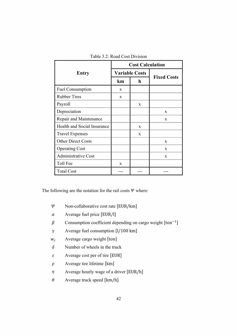
Table 3.2: Road Cost Division
Entry
Cost Calculation
Variable Costs Fixed Costs
km h
Fuel Consumption x
Rubber Tires x
Payroll x
Depreciation x
Repair and Maintenance x
Health and Social Insurance x
Travel Expenses x
Other Direct Costs x
Operating Cost x
Administrative Cost x
Toll Fee x
Total Cost --- --- ---
The following are the notation for the rail costs where:
Non-collaborative cost rate EUR/km
Average fuel price EUR/l
Consumption coefficient depending on cargo weight ton
γ Average fuel consumption l/100 km
Average cargo weight ton
Number of wheels in the truck
Average cost per of tire EUR
ρ Average tire lifetime km
Average hourly wage of a driver EUR/h
Average truck speed km/h

43
Percentage of wage for health and social insurance %
л Travel expenses EUR/h
Average original cost of truck EUR
Average lifetime of a truck year
Average operating time per truck per year hours/year
Average cost of maintenance and repairs per truck per year EUR/year
Toll fee per kilometer EUR/km
ξ Operating cost per year EUR/year
π Administrative cost per year EUR/year
ρ Other direct costs per year (insurance, material, etc.) EUR/year
The rail costs can then be represented as:
∙ ∙γ100
∙∙ρ
∙ι
100 л∙ ∙ ∙
ξ∙
π∙
ρ∙
(3.2)
The following section introduces the transfer costs equation.
3.4 Transfer Costs
The transfer costs can be divided into fixed and variable. They may depend upon the
transfer point at which they occur, as well as the incoming and outgoing modes at a transfer
point. The fixed costs depend mainly on the original construction cost of a terminal. This may
vary based on used technology of transshipment and handling equipment. Other fixed cost
elements are the operational and administrative cost. Variable costs are expenses that change
according to volume of service in a terminal, such as costs of manual workers, costs of consumed
material and etc. The total transfer cost per one unit of cargo is directly dependent on variable
costs and indirectly on fixed costs. The most important issue for minimizing the total price of

44
transfer per one unit is to reach the maximum capacity of a multimodal transfer facility. The
following table illustrates the cost breakdown for the transfer costs followed by the notation and
road cost equation.
Table 3.3: Transfer Cost Division
Entry
Cost Calculation
Variable Costs Fixed Costs
unit clearance
Payroll x
Consumed Material x
Depreciation of Terminal Construction x
Depreciation of Handling Equipment x
Repair and Maintenance of a Terminal x
Repair and Maintenance of a Handling Equipment x
Health and Social Insurance x
Other Direct Costs x
Operating Cost x
Administrative Cost x
Total Cost --- ---
The following are the notation for the rail costs where:
Transfer cost rate EUR/unit
Average hourly wage of a manual worker EUR/h
Number of loaded/unloaded units per hour unit/h
Percentage of wage for health and social insurance %
л Materials consumed during loading/unloading a unit EUR/unit
Construction cost of a terminal EUR
Average lifetime of a terminal year
Average number of loaded/unloaded units per year unit/year

45
Cost of handling equipment EUR
Average lifetime of handling equipment year
Average cost of maintenance and repairs of a terminal per year EUR/year
ε Average cost of maintenance and repairs of handling equipment per year
EUR/year
ξ Operating cost per year EUR/year
π Administrative cost per year EUR/year
ρ Other direct costs per year (insurance, material, etc.) EUR/year
The rail costs can then be represented as:
∙ι
100 л∙ ∙
ε ξ π ρ (3.3)
3.5 Summary
In summary, the cost calculations that were presented above provide a calculation
structure in order to transform the costs of all activities for calculation of core business activities
per one specific unit. These activities are transportation of trailers for road and rail operators and
transshipment of a trailers for multimodal terminal operators. In the case of rail transportation, it
is necessary to mention that the method of calculation radically differs in Europe and USA
because of different structures of rail infrastructure ownership. The infrastructure is owned by
rail companies in USA in contrast with Europe where the rail infrastructure is owned by states.
Also among the European countries can be found differences in rail cost calculation caused by
variation in charge policy.
The presented calculation models do not include the profit element. The main purpose of
this chapter was to develop a model of core cost calculations for transportation and transfer
operators. For the calculation of total price that should be charged to shipper the calculation

should
price is
include the
showed on
e profit elem
Figure 3.2.
ment also th
Figure
46
he VAT el
e 3.2: Total
ement, resp
Price Struc
pectively. C
cture
Complete strructure of

47
Chapter 4: A MULTIMODAL FREIGHT COLLABORATIVE HUB LOCATION
PROBLEM
Chapter 4 introduces the formulation of the multimodal freight collaborative hub location
problem addressed in the thesis. Section 4.1 introduces the problem. The mathematical model is
developed in Section 4.2. This section presents the sets and indices, parameters, and defines the
decision variables. This section also provides the set of constraints and defines the objective
function. Section 4.3 provides some concluding comments for Chapter 4.
4.1 Introduction
When one is selecting a location for the multimodal facilities, it is necessary to proceed
systematically, as it is a crucial decision, i.e. later unchangeable. The most important factor that
influences the choice of a location for the establishment of a multimodal terminal is the existing
transportation infrastructure network. Logistics centers cannot function effectively without
efficient connections to a network of good quality and transportation infrastructure. In the case of
a multimodal collaborative effort, such as rail-road collaboration, the need for facilities that can
accommodate and facilitate collaboration is of great importance. So the problem becomes one of
establishing (i.e., identifying) collaborative facilities that can support a rail-road collaborative.
The following sections are our attempts to formulate the multimodal freight collaborative hub
location problem (MFCHLP).
4.2 Mathematical Model, Problem Description and Assumptions
The MFCHLP seeks to determine a set of multimodal consolidation collaborative
consolidation transshipment hubs for a rail-road collaboration that minimizes the total
collaborative costs for the set of collaborating carriers (both the rail and road-based freight

48
carriers). Hence, a carrier in this system is classified as either a collaborative carrier (shares the
costs to set up multimodal hubs), or non-collaborative (decides to ship directly). The operational
networks of the collaborating carriers can be completely identical geographically or overlap in
some segments relative to other carriers in the collaborative.
The collaborative rate structure of the collaborative carriers is represented by
revenue oriented behavior. If a collaborative opportunity cannot be identified with regards to the
multimodal collaborative hubs, a non-collaborative option is considered. It is assumed that the
costs of shipping directly fall upon the carrier itself.
The following assumptions are made in the MFCHLP: (i) candidate multimodal
collaborative consolidation hubs are uncapacitated, and (ii) heterogeneous products are shipped.
In addition, the problem is deterministic in the sense that the demand is known and the available
holding times at facilities are time invariant. By contrast, a stochastic version of the problem
would entail stochasticity of demand of the collaborating carriers.
4.2.1 Indices and Sets
In MFCHLP formulation, a shipment from collaborative carrier ∈ enters the
collaborative network through an origin facility ∈ ⊆ N and travel via multimodal
consolidation candidate transshipment hubs , ∈ and exit through a destination facility
∈ ⊆ N. Let represent the number of trucks (or shipments) utilized by collaborative
carrier ∈ from origin facility ∈ ⊆ N to destination facility ∈ ⊆ N.
4.2.2 Parameters
Let be the collaborative carrier ∈ revenue oriented cost associated to a unit of
demand to travel between origin facility ∈ to destination facility ∈ when going via
multimodal consolidation candidate transshipment facilities at node ∈ and ∈ .

49
In addition, denotes the cost for collaborative carrier ∈ to establish a facility at
node ∈ . Note that a collaborative carrier may choose to ship directly without
participating in the multimodal collaborative network if the collaborative cost is not significantly
lower than the direct shipping cost, . Furthermore, a facility is established only if that
facility has the capability to provide capacity for collaborative transshipment to take place, and
this capacity is represented by , .
The maximum number of hubs opened is given by the parameter .
4.2.3 Decision Variables
The formulation has three sets of binary decision variables:
(i) takes the value 1 if shipment originating from ∈ headed to destination
∈ by collaborative carrier ∈ travel via multimodal consolidation candidate
transshipment hubs ∈ and ∈ and 0 otherwise,
(ii) takes the value 1, if carrier q ships the demand directly without
participating in the collaboration and 0 otherwise,
(iii) takes the value 1 if a multimodal consolidation candidate transshipment hub is
located at node ∈ and 0 otherwise.
4.2.4 Constraints
∈
∀ ∈ (4.1)
∈∈
1 ∀ ∈ , ∈ , ∈ (4.2)
∈
, ∀ ∈ , ∈ , ∈ , ∈ (4.3)

50
∈
∀ ∈ , ∈ , ∈ , ∈ (4.4)
1 1 ∀ ∈ , ∈ , ∈ , ∈ , ∈ (4.5)
∈ 0,1 , ∈ 0,1 , ∈ 0,1 ∀ ∈ (4.6)
Constraints (4.1), (4.2), (4.3), (4.4) ensure the consistency between facility location and
collaborative routing , i.e., shipments are routed through hub l only if a facility is established
there. Constraint (4.2) and (4.5) ensures that a shipper will not participate in collaboration unless
it is significantly lower than the direct routing costs.
4.2.5 Objective Function
The objective function of the MFCHLP minimizes the sum of transportation and
construction costs generated by facility location. The objective function is represented as:
∈∈∈∈∈ ∈∈∈ ∈∈
(4.7)
It consists of three parts. The firs term represents the total shipment costs of carrier
collaborating in multimodal transportation, second term represents the non-collaborating case
and the last term represents the costs of multimodal hub terminals located in the network. The
overall collaborative costs are obtained as the summation of collaborative rate , the demand
, and (the decision on whether collaboration is costly more efficient than direct
shipping). The overall non-collaborative costs are obtained as the summation of the non-
collaborative rate , the demand , and (the decision on whether the direct shipping is
costly more efficient than collaborative shipping). The overall costs of establishing the transfer
facility in network are obtained as the summation of cost of establishing the facility , and
(the decision on whether the establishing of facility is effective).

T
1995). S
exact m
mention
sophisti
etc.).
F
The MFCH
Since, these
method to s
ned earlier
cated soluti
Figure 4.1 i
HLP is know
are the firs
solve the pr
additiona
ion approac
s an illustra
F
wn to be NP
st attempts o
roblem, nam
al dimensio
ches such as
ation of the d
Figure 4.1: L
51
-hard as it r
of formulatin
mely the br
ons such
s meta-heur
decision pro
Location Mo
reduces to a
ng the MFC
ranch-and-c
as time-de
ristics (e.g.,
ocess for the
odel Schema
a p-median p
CHLP (whic
cut algorithm
ependency
genetic alg
e MFCHLP
atic
problem (se
ch is static)
m (see CPL
will requ
gorithms, tab
:
ee Daskin,
we use an
LEX). As
uire more
bu search,

52
4.3 Summary
The developed location model offers an optimization tool that can be used by decision-
makers in the framework of a multimodal network. This tool can compute optimal locations of a
determined number of hubs and show changes of adding additional hubs in the network. The
schematic of proposed model is illustrated in Figure 4.1.
53
Chapter 5: A COLLABORATIVE FREIGHT MULTIMODAL FIXED CHARGED
NETWORK DESIGN PROBLEM
Chapter 5 discusses the collaborative freight multimodal fixed charged network design
problem addressed in the thesis. Section 5.1 describes the problem generally. Section 5.2
introduces the mathematical model, this includes formulation of sets and indices, calculation of
input parameters and decision variables, finding of the limiting constraints, and formulation of
objective function. Section 5.3 provides some concluding comment for this chapter.
5.1 Introduction
Fixed charged network design models are extensively used to present a wide range of
planning and operation decision- making issues in transportation, telecommunications, logistics,
and production. The basic approach of solving the collaborative freight multimodal fixed
charged network design problem is from the point of view of the carrier. Compared to all
previous models, the carrier here is offered an alternative route of rail transportation that might
lower the total costs. This problem is called Static Multimodal Collaborative Carrier Problem
(SMMCCP) and its formulation is presented in following chapter.
5.2 Mathematical Model, Problem Description and Assumptions
The SMMCCP seeks the appropriate network design from the predefined set of networks,
to determine the routing for each O-D pair which minimizes the total transportation cost. Hence,
the carrier of interest may use some free capacity from various multimodal train operators for the
segments of route on which rail mode of transportation is available. Since this problem is static
in the sense that the demand is constant and the available capacities from the collaborative

54
carriers are time invariant, a dynamic version of the SMMCCP would entail the availability of
time-dependent collaborative capacities from the collaborative carriers and train operators.
The collaborative rate structure of the collaborative carriers is represented by revenue
oriented behavior. If a collaborative opportunity cannot be identified with regards to the
collaborative network design, a non-collaborative option is considered. It is assumed that the
costs of shipping directly fall upon the carrier itself.
5.2.1 Indices and Sets
Let , denote an undirected network with node set and link set . The index
denotes a node in the network, ∈ and ∈ ⊆ , where denotes an undirected link
that originates from the facility ∈ is depicted as ∈ Г and this heading to facility ∈ is
∈ Г with nonnegative fixed costs. Let a shipment ∈ be served by a transit corridor
∈ through multimodal collaborative route served by carrier ∈ and by multimodal train
∈ or through non-collaborative road served just by carrier ∈ . Fixed transshipment
facilities ∈ , collaborative carriers ∈ and multimodal trains ∈ form a collaborative
network. A shipment ∈ will enter the collaborative network through an origin facility
and exit through a destination facility . For each shipment ∈ there is its origin-
destination pair that origins in the facility and directs to the destination facility .
5.2.2 Parameters
Each shipment ∈ has an associated volume . The cost for acquiring a unit of
capacity from collaborative multimodal transshipment via carrier ∈ utilizing train ∈ on
transit corridor ∈ is a collaborative rate . The fixed cost for transferring shipment to or
from the train is included in the collaborative rate . If the carrier does not use the
collaborative transshipment, the non-collaborative rate is .

55
The available collaborative capacity of a multimodal train ∈ for transit corridor
∈ is . If a multimodal collaboration of train ∈ is not provided for transit corridor
∈ , it is assumed without loss of generality that available collaborative capacity is 0.
5.2.3 Decision Variables
If shipment ∈ takes place on transit corridor ∈ to non-collaborative carrier
∈ , one defines to take the value of 1, and 0 otherwise. It represents the non-
collaborative shipment transfer decision variable for the carrier of interest.
If a shipment ∈ is served through transit corridor ∈ by carrier ∈ utilizing
multimodal train ∈ , one defines to take the value of 1, and 0 otherwise. The variable
represents the multimodal collaborative capacity for the carrier of interest.
5.2.4 Constraints
The formulation of constraints of SMMCCP consists of two sets of constraints. The first
set of constraints (5.1; 5.2; and 5.3) model the independent transshipment of shipment through
the collaborative route. The second set of constraints (5.4) establishes a limitation on the
available collaborative capacity (or number of wagons) made available by train ∈ on transit
corridor ∈ . The constraints are as followed:
∈
1∈∈
∀ ∈ , ∈ 5.1
∈∈ ∈∈∈
0∈
∀ ∈ \ , , ∈ 5.2
∈∈∈
1 ∀ ∈ , ∈ 5.3

56
∈∈
∀ ∈ , ∈ 5.4
1 1 ∀ ∈ , ∈ , ∈ , ∈ 5.5
∈ 0,1 ∀ ∈ , ∈ , ∈ 5.6
∈ 0,1 ∀ ∈ , ∈ , ∈ 5.7
Constraint set (5.1; 5.2; 5.3) represents the mass balance constraints and ensures the node
flow propagation conservation for multimodal transportation shipment decisions; at most one
decision unit of multimodal transport shipment is propagated at that facility. It consists of (5.1),
(5.2), and (5.3), which correspond to the origin, intermediate, and destination nodes/facilities in
the network, respectively.
Constraint (5.4) represents the train mode capacity constraint; it ensures that the capacity
acquired from a carrier (left-hand side of (5.4)) is less than the available train mode capacity
(right-hand side of (5.4)) on that transit corridor. Constrain (5.5) reflects the marginal effect
through parameter Constraint sets (5.6) and (5.7) represent the 0-1 integrality conditions for
the decision variables.
5.2.5 Objective Function
The objective function of the SMMCCP seeks to minimize the total multimodal
collaborative costs for multiple carriers and is represented as:
∈∈∈ ∈∈∈∈
5.8
It consists of two parts. The first term represents the total shipment costs of carriers not
collaborating, and the second term represents the multimodal collaborative transaction costs

57
between a carrier and rail company. The overall non-collaborative costs are obtained as the
summation of non-collaborative cost , the demand , and the decision variable on
whether the direct shipping is more effective than collaboration. The overall collaborative costs
are obtained as the summation of collaborative rate , the demand , and the decision
variable , that has value 1 if the collaborative route is costly efficient. In contrast of
previous model, the fixed component of transfer cost is included in collaboration rate and the
variable element as well.
The SMMCCP is known to be NP-hard as the problem size increases (see Ahuja et al.,
1993; Hernandez and Peeta, 2010). Since, these are the first attempts of formulating the
SMMCCP (which is static) we use an exact method to solve the problem, namely the branch-
and-cut algorithm (see CPLEX). As mentioned earlier additional dimensions such as time-
dependency will require more sophisticated solution approaches such as meta-heuristics (e.g.,
genetic algorithms, tabu search, etc.).
Figure 5.1 is an illustration of the decision process for the SMMCCP:

5.3 S
T
transpor
routing
that ent
provide
routing
location
enables
Summary
The networ
rtation scien
in a networ
er the mode
s as its out
(path) for t
n of facilitie
to identify t
Figur
rk design p
nce. The d
rk system th
el are the c
tput the cal
transshipme
es and netw
the best rou
re 5.1: Netw
problem pro
developed r
hat achieves
cost input p
lculation of
ent of each
work design
uting of colla
58
work Design
ovides anoth
routing mod
s the minim
parameters a
f total costs
commodity
n model, ba
aborative sh
n Model Sch
her perspec
del allows
mization of c
and the netw
s generated
y. The hub
ased on spec
hipments.
hematic
tive of opti
users to de
costs. The o
work data.
by the sys
location m
cific locatio
imization s
etermine th
only input p
The present
stem and th
model determ
ons of facil
olution in
he optimal
parameters
ted model
he optimal
mines best
ities, then

59
Chapter 6: APPLICATION OF MODELS
This chapter discusses computational experiments using test networks to seek insights on
the performance of developed models as well as on the implications for practical applications.
Section 6.1 discusses the data generation. Section 6.2 describes the 3 different size test networks.
Section 6.3 discusses experiments and insights on model application using several test options.
In Section 6.4 is provided the sensitivity analysis for key model parameters. The chapter
concludes with a summary of the application insights.
6.1 Data Generation
The data needed for running the hub location experiment consist of cost matrices of
collaborative routes, demand matrices, matrices that represent the cost to establish a facility as an
intermodal collaborative facility, cost matrices of non-collaborative route, and matrices of rail
capacities.
The network design model requires different set of input data. The set of rail capacities
has to be defined. Another important modification can be found in demand. Demand is
represented as a set of commodities that originate at a node i and destined to a node j. All
demand data are formed in 3 matrices. The first one represents the value of commodity for each
carrier; the other two matrices define the origin and destination nodes for each type of
commodity. The network is defined in two separate matrices. The first one is the node-arc
adjacency matrix and the second is the matrix in which is listed the set of arcs of the network.
The data generation of each input matrix is discussed below.
60
6.1.1 Non-collaborative route cost matrix
The non-collaborative cost matrix represents the cost of usage of road infrastructure. The
costs matrices for each arc in the road network was created by multiplying the arc distance by the
road cost parameter. The cost parameter varied between 0.95 and 1.05 was used to present the
possible differentiation of costs for each route.
Also, the same data generation method for network design model was utilized. The only
difference is that the road cost for each arc and each carrier were defined. In the previous model
was used the same road cost for all carriers.
6.1.1.1 Road Cost Parameters
The calculation of road cost per kilometer is based on equation 3.2. This equation
calculates the total road cost of transportation per 1 kilometer. The equation covers all costs that
occur during the road transportation. All parameters are listed in Table 6.1. The input parameters
in this experiment try to mimic the current conditions of road transportation in Czech Republic.

61
Table 6.1: Road Cost Input Parameters
Parameters Units Monetary Value
Fuel Consumption l/100km 38
Fuel Price Eur/l 1.45
Consumption Coefficient ton-1 0.04
Cargo weight ton 25
Tire Cost Eur/peace 245
Number of Tires pieces 12
Tires Run Over km 50,000
Wage Eur/h 10
Price of the Truck Eur 110,000
Lifetime of the Truck years 6
Repair and Maintenance Eur/year 0.15
Health and Social Insurance % of salary 31
Travel Expenses Eur/h 0.26
Truck Insurance Eur/year 2300
Toll Fee Eur/km 0.2
Operating Cost Eur/year 1,900
Administrative Cost Eur/year 1,600
Truck Operating Time hours/year 2,200
Truck Speed km/h 80
The diversification of cost components is listed in Table 6.2 and its graphical
representation is illustrated on Figure 6.1.

Table 6
Fuel C
Rubbe
Payrol
Deprec
Repair
Health
Travel
Other
Operat
Admin
Toll F
Total
6.2: Road C
Entry
Consumption
er Tires
ll
ciation
r and Mainten
h and Social I
l Expenses
Direct Costs
ting Cost
nistrative Cos
ee
Cost
Figure 6.1
62
Cost Compon
y
nance
Insurance
s
st
1: Road Cos
nents Diver
EUR
0.55
0.04
0.12
0.10
0.15
0.03
0.00
0.01
0.01
0.00
0.20
1.25
sts Structure
sification
R/km
1000000
49000000
5000000
04166667
0000000
8750000
03250000
3068182
0795455
09090909
00000000
54121212
e

63
6.1.2 Collaborative route cost matrix
This costs matrix represents the costs of transshipping of one freight unit from node to
node through multimodal facilities l and m. The usage costs for each arc in the rail network
were created by multiplying the arc distance by the rail cost parameter. The costs of the
collaborative routes include also the variable component of transfer costs that occur during a
transfer at a facility. The cost parameter varied between 0.95 and 1.05 to represent the possible
differentiation of costs for each rail route.
The routing model requires slight modification, that is, the collaborative cost includes not
just the variable component of transfer cost, but also the fixed cost that covers also the cost to
establish the facilities. The structure of collaborative matrix was extended and involves the
collaborative cost of each arc for combination of each carrier that can collaborate with a rail
mode.
6.1.2.1 Rail Cost Parameters
The calculation of rail cost per one kilometer was more complicated than the calculation
of the road-based costs. Big rail companies usually do not publish their internal information
about cost calculations but, with cooperation of Czech national cargo operator (CD Cargo) it was
possible to determine approximate cost parameters. They are listed in Table 6.3.

64
Table 6.3: Rail Cost Input Parameters
Parameters Units Monetary Value
Energy Consumption kWh/1,000 gross ton km 20
Energy Price Eur/kWh 0.18531
Weight of a Locomotive ton 80
Weight of a Wagon ton 20
Weight of a Trailer ton 7
Cargo Weight ton 25
Cost of Operating Infrastructure Eur/km 0.98
Maximal Length of Train m 700
Length of a Locomotive m 20
Length of a Wagon m 20
Cost for Ensuring the Operability of Infrastructure Eur/1,000 gross ton km 1.30
Wage Eur/h 14
Price of a Locomotive Eur 3,250,000
Lifetime of a Locomotive years 20
Price of a Wagon Eur 280,000
Lifetime of a Wagon years 18
Cost of Maintenance and Repairs of a Locomotive Eur/year 50,000
Cost of Maintenance and Repairs of a Wagon Eur/year 2,000
Health and Social Insurance % of salary 31
Travel Expenses Eur/h 0.26
Other Direct Costs Eur/year 20,000
Operating Cost Eur/year 50,000
Administrative Cost Eur/year 15,000
Locomotive Operating Mileage km/year 140,000
Wagon Operating Mileage km/year 180,000
Train Speed km/h 100
The individual components of calculation equation 3.1 are provided in Table 6.4. The
cost structure is illustrated in Figure 6.2.

Energy
Payroll
Deprec
Deprec
Repair
Repair
Health
Travel
Other D
Operat
Admin
Cost of
Cost fo
Total C
Table
y Consumptio
l
ciation of Loc
ciation of Wa
and Mainten
and Mainten
and Social In
Expenses
Direct Costs
ing Cost
nistrative Cos
f operating in
or ensuring th
Cost
6.4: Rail Co
Entry
on
comotive
agon
nance of Loc
nance of Wag
nsurance
st
nfrastructure
he operability
Figure 6.
65
ost Compon
omotive
gon
y of Infrastru
2: Rail Cost
nents Divers
ucture
ts Structure
sification
EUR/k
0.2014
0.0041
0.0341
0.0864
0.0108
0.0115
0.0012
0.0000
0.0042
0.0105
0.0033
0.0288
0.0706
0.4674
km
442871
117647
138655
419753
869748
533333
276471
076471
201681
504202
361345
823529
658824
42452

66
6.1.2.2 Transfer Cost Parameters
The calculation of transfer cost per one cargo unit covers equation 3.3. The parameters
are based on estimation. It is not possible to get accurate parameters that could be based on
realistic information, because the considered multimodal technologies are still under
development. The Table 6.5 provides the estimation of parameters that occur in mathematical
equation.
Table 6.5: Transfer Cost Input Parameters
Parameters Units Monetary Value
Wage Eur/h 8
Loaded/unloaded units per hour unit/hour 6
Health and Social Insurance % of salary 31
Materials consumed during loading a unit Eur/unit 0.5
Construction cost of terminal Eur 4,000,000
Lifetime of the terminal years 20
Average number of loaded/unloaded units per year unit/year 20,000
Cost of handling equipment Eur 250,000
Lifetime of the handling equipment years 7
Cost of repair and maintenance of a terminal per year Eur/year 90,000
Cost of repair and maintenance of handling equipment per year Eur/year 10,000
Operating Cost Eur/year 50,000
Administrative Cost Eur/year 30,000
Other direct costs per year Eur/year 60,000
Table 6.6 provides the diversification of cost components and the cost structure is shown
on Figure 6.3.

Payroll
Consume
Depreciat
Depreciat
Repair an
Repair an
Health an
Other Dir
Operating
Administr
Total Co
Total Co
Table 6.6
d Material
tion of Termi
tion of Handl
nd Maintenan
nd Maintenan
nd Social Insu
rect Costs
g Cost
rative Cost
st
st per unit
6: Transfer
Entry
inal Construc
ling Equipme
nce of a Term
nce of a Hand
urance
Figure 6.3:
67
Cost Comp
ction
ent
minal
dling Equipm
Transfer Co
onents Dive
Fixed
EUR/
200,0
35,7
90,0
ment 10,0
60,0
50,0
30,0
47,57
osts Structu
ersification
Costs Var
R/year E
000.00
714.28
000.00
000.00
000.00
000.00
000.00
714.28
26.03
ure
riable Costs
EUR/unit
1.33
0.50
0.41
2.24

6.1.3 T
T
6.5 and
arcs tha
The val
calculat
generate
6.1.3.1 6
T
The tota
on Figur
The Test N
Three differ
6.6. The ne
at represent t
lues represe
tions is dem
ed and all gr
6-node Netw
The smalles
al length of
re 6.4.
Networks
rent size net
etworks con
the road (lig
ent the mile
monstrated b
raphs are ac
work
st test netw
f roads is 1,7
tworks were
nsists of nod
ght blue line
eages betwe
by use of di
cyclic.
work consist
789 km and
Figure 6
68
e created ra
des that repr
es) and rail
een nodes i
fferent size
ts of 6 node
d length of r
6.4: 6-nodes
andomly. Th
resent the o
(dark red lin
in kilomete
of network
es and seve
rails is 1,32
s Network
hey are illus
origin and d
nes) connec
ers. The dif
ks. The netw
eral connect
24 km. The
strated in Fi
estination p
ctions betwe
fferent comp
works were
tions betwe
network is
igures 6.4,
points, and
een nodes.
mplexity of
randomly
een nodes.
illustrated

6.1.3.2 1
M
3,273 k
Figure 6
6.1.3.3 1
T
roads an
12-node Ne
Medium siz
km and the
6.5.
18-node Ne
The biggest
nd 3,222 km
etwork
ze network
length of ra
etwork
t test networ
m of rails. Th
was extend
ails was ext
Figure 6
rk is compo
he 36-node
69
ded to 18 n
tended to 2
6.5: 12-node
osed of 18 n
network is i
nodes netwo
2,578 km. T
es Network
nodes that ar
illustrated o
ork. The tot
The network
re interconn
on Figure 6.6
tal length o
k design is
nected by 4,8
6.
of roads is
shown on
804 km of

6.1.4 D
T
in one y
experim
T
two mat
model f
6.1.5 C
T
facility
Demand
The demand
year. The v
ments consid
The demand
trices are de
five carriers
Cost matrix
This matrix
for each ca
d matrix rep
values were
der three car
d is defined
efined to ide
and several
x to establi
x represents
arrier. The v
Figure 6
presents the
generated r
rriers of inte
as a combi
entify the o
l types of co
sh a facility
s the costs
values vary
70
6.6: 18-node
e number of
randomly b
erest and one
nation of co
origin and de
ommodities
y as an inte
to establish
y from the f
es Network
f trailers (co
between 100
e type of co
ommodity a
estination n
are conside
ermodal col
h a facility
fixed eleme
ontainers) sh
00 and 2000
ommodity.
and a carrier
nodes of eac
ered.
llaborative
as an inte
ent of calcu
hipped by t
0 units per
r. That is wh
ch commodi
facility
ermodal col
ulated transf
the system
year. The
hy another
ity. In this
llaborative
fer cost in

71
equation 3.3. The values were randomly generated from 200,000 Euros and 400,000 Euros per
year.
6.1.6 Matrix of rail capacities
Each established multimodal collaborative facility has a capacity limitation. Therefore,
the limit of passing units per year for each node in the network is defined.
In contrast to previous models, there is defined a set of 5 train operators that offer their
train capacity to carrier. The train capacity is not defined just for each node in the network but,
for each combination of arc and train operator.
6.2 Computational resources
The computing environment consists of a IBM Lenovo ThinkPad T61 with Intel®
Core™2 Duo CPU processor under the Windows 7 64-bit Ultimate operating system with 4 GB
of RAM. The server device with 2 X5680 3,33 GHz processors of Intel® Xeon® CPU under
Windows 7 64-bit Enterprise operating system with 8 GB of RAM was used for more complex
processes. The GAMS/CPLEX version 22.9.2 was used.
6.3 Experiments setup
There are 4 possible collaboration scenarios in experiments that are illustrated on Figure
6.7. The collaboration route can take whole route if i=l and j=m. This case is shown on
illustration A. The rail mode of transportation is used through the whole route. The collaborative
route will take place most likely in the middle of the route; this case is illustrated in C. The last
combination is shown on illustrations D and F. The collaborative portion takes place either at the
beginning of the route or at the end. The condition that i=l or j=m must be satisfied. B illustrates
the non-collaborative route.

Figure 6.7: T
72
The collaborration scenarios

73
6.4 Experiments
The potential for collaboration among multimodal network is investigated by focusing on
the level of monetary savings due to the collaboration. The level of collaboration is reflected
through the number of established multimodal facilities, which takes values from 0 to the value
when the total costs start to go up. On the basis of the calculations, one can determine the best
allocations of multimodal facilities and their optimal number. The following sections highlight
the results under varying network conditions.
6.4.1 6 node network hub location experiment
As seen in Table 6.7, the total costs decrease even when two facilities are established.
However, the value of objective function increases if 4 or more hubs are established. This is
caused by increasing costs to establish multimodal facilities that exceed savings from
collaboration. Costs performance is illustrated in Figure 6.8. The optimal solution for 6-node
network is establishing 3 multimodal facilities in nodes 2, 4, and 5 as is illustrated in Figure 6.9.
The costs structure of optimal solution is shown on Figure 6.10.

Table
No. of located facilities
No co
2
3
4
5
6
6.7: The Co
s Location
ollaboration
2,4
2,4,5
1,2,4,5
1,2,4,5,6
1,2,3,4,5,6
Figure
omparison o
ns
Costsestabltrans
facilitie
0
1,400,31
2,173,43
3,049,36
3,963,29
6 4,942,88
6.8: The co
of different s
s to lish sfer es [€]
collaco
0.00 19,68
5.00 9,06
3.00 5,74
5.00 3,09
1.00 1,82
3.00 1,364
omparison o
74
scenarios ofne
Non-aborative osts [€]
5,809.00
3,489.00
8,154.00
3,446.00
1,155.00
4,001.00
f the costs p
f number ofetwork
Collaboraticosts[€]
0.00
4,540,001.00
6,278,979.00
8,207,928.00
9,412,784.00
9,853,660.00
performance
f established
ive Total [€
0 19,685,80
0 15,003,80
0 14,200,56
0 14,350,73
0 15,197,23
0 16,160,54
e for 6-node
d facilities in
costs €] imp
09.00
05.00
66.00
39.00
30.00
44.00
e network
n 6-node
Cost rovement
0
23.78 % 1
5.35 % 1
-1.06 % 0
-5.90 % 0
-6.34 % 0
CPU time
[s]
0.10
1.04
1.46
0.48
0.59
0.15

6.4.2 1
T
perform
collabor
Figure 6.
Figure 6
12 node net
The optima
mance is liste
rative costs
C
9: The optim
6.10: The co
twork hub
al solution
ed in Table
become co
Costs st
mal location
osts structur
location ex
n in 12-no
6.8 and illu
onstant afte
ructure
75
n of 3 multim
re of the opt
xperiment
ode network
ustrated in F
er 7 or mor
of the o
modal facili
timal solutio
k is 6 mu
igure 6.11.
re facilities
optimal
ities in 6-no
on in 6-node
ultimodal f
The collabo
are establi
l solutio
Collabora
Non‐colla
Costs to emultimod
ode network
e network
facilities. T
orative costs
ished. This
on
ative Costs
aborartive Co
establishdal facilities
k
The costs
s and non-
is caused
osts

76
either by utilization of all available rail capacity or the possibility of effective use of
collaborative routes between specific O-D pairs. The optimal locations of hubs are in nodes
1,2,6,8,10 and 12 as illustrated in Figure 6.12. The costs structure of this solution is shown on
Figure 6.13.
Table 6.8: The comparison of different scenarios of number of established facilities in 12-node network
No. of located facilities
Locations
Costs of establishing the transfer facility [€]
Non-collaborative
costs [€]
Collaborative costs [€]
Total costs [€]
Cost improvement
CPU
time [s]
No collaboration 0.00 37,527,848.00 0.00 37,527,848.00 1.99
2 1,6 1,586,626.00 24,164,555.00 5,814,052.00 31,565,233.00 15.89% 35.36
3 1,6,8 2,432,510.00 18,904,777.00 8,023,174.00 29,360,461.00 6.98% 24.02
4 1,2,6,8 3,430,021.00 14,046,485.00 10,551,598.00 28,028,104.00 4.54% 56.23
5 1,2,6,8, 12
4,215,889.00 10,858,606.00 11,890,199.00 26,964,694.00 3.79% 41.75
6 1,2,6,8,
10,12 5,005,579.00 8,128,872.00 13,008,931.00 26,143,382.00 3.05% 36.46
7 1,2,5,6,8,
10,12 5,849,413.00 4,468,932.00 16,244,723.00 26,563,068.00 -1.61% 6.47
8 1,2,5,6,8,
9,10,12 6,681,167.00 4,468,932.00 16,244,721.00 27,394,820.00 -3.13% 7.94
9 1,2,3,5,6,
8,9,10,12 7,548,370.00 4,468,932.00 16,244,722.00 28,262,024.00 -3.17% 9.92
10 1,2,3,4,5,
6,8,9,10,12 8,747,506.00 15,626,878.00 18,361,043.00 29,207,844.00 -1.78% 184.74

Figure 6
Figure 6.1
6.11: The co
2: The optim
omparison o
mal location
77
f the costs p
n of 6 multim
performance
modal facili
e for 12-nod
ities in 12-n
de network
node networrk

6.4.3 1
T
locating
are esta
and 18.
collabor
establish
facility.
problem
computa
sites.
Figure 6
18 node net
Table 6.9 i
g specific nu
ablished in t
The graphi
rative and
hed. Therea
Final costs
m is NP-har
ational expe
6.13: The co
twork hub
illustrates th
umbers of m
this network
ical represen
non-collab
after the tota
s structure
rd the less t
ense was ob
The c
osts structure
location ex
he results o
multimodal
k. The alloc
ntation is il
orative cos
al costs depe
of best solu
the number
bserved. Thi
osts stru
78
e of the opti
xperiment
of the costs
facilities. T
cation of op
llustrated in
sts become
end only on
ution is sho
r of facilitie
is is due to
ucture osolution
imal solutio
s performan
The lowest t
ptimal solut
n Figure 6.1
e constant
n marginal c
own on Fig
es needed t
greater num
of the on
on in 12-nod
nce for the
total costs a
tion is in no
5. As show
after 9 or
ost to establ
gure 6.16. J
to be establ
mber of com
ptimal
Collaborat
Non‐collabCosts
Costs to esmultimoda
de network
18-node ne
are reached
odes 1,2,6,8
wn in Figure
more faci
lish other m
Just a note,
lished the g
mbinations o
tive Costs
borartive
stablishal facilities
etwork by
d if 8 hubs
8,11,13.16
e 6.14, the
ilities are
multimodal
since the
greater the
of possible

Table 6
No. of located facilitie
s
No co
2
3
4
5
6
7
8
9
10
6.9: The com
Locations
ollaboration
2,6
2,6,13
2,6,7,13
1,2,6,7,13
1,2,6,8,13,
18
1,2,6,8,13,
16,18
1,2,6,8,11,
13,16,18
1,2,6,8,11,
13,14,16,18
1,2,6,7,9,11
13,14,16,18
Figu
mparison of
s
Costs oestablishthe tranfacility
1,933,54
2,850,26
3,796,72
4,596,46
5,464,32
6,413,51
7,203,73
8 7,999,22
1,
8 8,747,50
ure 6.14: The
f different s
of hing sfer [€]
Ncollab
cos
0.00 54,71
46.00 39,95
62.00 34,36
27.00 29,69
65.00 23,07
23.00 20,03
10.00 17,34
37.00 16,06
21.00 15,62
06.00 15,62
e compariso
79
cenarios of ne
Non-borative sts [€]
C
14,761.00
52,709.00 6
60,859.00 9
93,983.00 11
78,624.00 15
34,307.00 16
44,362.00 17
69,206.00 17
26,878.00 18
26,878.00 18
on of the co
number of eetwork
Collaborative costs [€]
0.00
6,381,513.00
9,103,028.00
1,057,023.00
5,218,020.00
6,508,921.00
7,597,705.00
7,993,130.00
8,361,043.00
8,361,043.00
sts performa
established
Total cost[€]
54,714,761
48,267,768
46,314,149
44,547,733
42,893,109
42,007,551
41,355,577
41,266,073
41,987,142
42,735,427
ance for 18-
facilities in
ts Improv
.00
8.00
9.00
3.00
9.00
.00
7.00
3.00
2.00
7.00
-node netwo
18-node
vement C
tim
11.78% 318
4.05% 46
3.81% 22
3.71% 8
2.06% 7
1.55% 4
0.22% 2
-1.75% 3
-1.78% 1
ork
CPU me [s]
25.77
802.55
633.41
272.39
809.57
723.96
423.48
278.99
331.32
184.74

Figure 6.15
Figure 6
Th
5: The optim
6.16: The co
e costs
mal location
osts structure
structur
80
ns of 8 multi
e of the opti
re of the
imodal facil
imal solutio
e optim
C
N
Cm
lities in 18-n
on in 18-nod
mal solut
Collaborativ
Non‐collabo
Costs to estamultimodal
node networ
de network
tion
ve Costs
orartive Cost
ablishfacilities
rk
ts

81
6.4.4 18 node network design experiment
The network design model was tested just on 18 node network; the reason is that we are
interested in the viability of collaboration through rail-road collaborative routes. In future work
we will consider larger networks and the issue of time-dependency. The experiment considers 5
carriers of interest and 5 collaborative train operators. This generates the possible combinations
of 25 collaborative pairs. The experiments were run with varying number of shipments from 20,
40, 60, respectively. The total costs and composition of collaborative and non-collaborative
routes is listed in Table 6.10. These results are a snapshot of the network design analysis. The
following sections we illustrate how collaborative rates can influences the routes taken and the
costs to the collaborative.
Table 6.10: The comparison of different scenarios of network design demand in 18-node network
Number of shipments
Total Costs
Non-collaborative
Costs
Collaborative Costs
Non-collaborative
routes
Collaborative Routes
CPU time
20 8,939,864 2,134,944 6,804,920 14 46 1.592
40 16,965,753 3,871,062 13,094,691 28 92 3.697
60 26,987,520 7,324,932 19,662,588 43 137 7.145
6.5 Sensitivity Analysis
In this section a sensitivity analysis is performed. Sensitivity analyses illustrate how
changes of certain input values (costs) produced due to inappropriate prediction or some other
reason , influence certain criteria values and the total costs (Janovic, 1999). The sensitivity
parameters are α (alpha), β (beta) and γ (gamma).
6.5.1 Collaborative discount rate for the MFCHLP problem
The sensitivity parameter α represents the discount rate of the collaborative part of route
for the MFCHLP problem. The discount parameter was established in range between 0 (no

82
discount) and 0.9 (90% discount). Table 6.11 shows the results for parameter α case of optimal
solution in 18-node network. This parameter can be represented in reality as a government
subvention or as the saving from usage of more efficient technology (e.g. lower cost of
depreciation or repair and maintenance costs). The graphical representation is shown in Figure
6.17. The analysis was performed for eight hubs (since 8 hubs were the optimal under default
values). The results indicate a decrease in total costs as alpha increases.
Table 6.11: Sensitivity analysis of optimal solution in 18-node network for the MFCHLP problem according to parameter α
No. of
hubs Alpha Locations
Collaborative Costs
Non-collaborative
Costs
Costs of establishing the transfer
facilities
Total Costs
8
0.0 1,2,6,8,11,13,16,18 17,993,129.00 16,069,206.00 7,203,737.00 41,266,072.00
0.1 1,2,6,8,12,13,16,18 17,740,173.00 16,069,206.00 7,272,762.00 41,082,141.00
0.2 1,2,3,6,8,12,13,18 16,281,518.00 17,209,563.00 7,297,064.00 40,788,145.00
0.3 1,2,3,6,8,12,13,18 15,619,661.00 17,209,563.00 7,297,064.00 40,126,288.00
0.4 1,2,3,6,8,12,13,18 14,957,802.00 17,209,563.00 7,297,064.00 39,464,429.00
0.5 1,2,3,6,7,8,13,17 13,940,966.00 17,344,362.00 7,472,744.00 38,758,072.00
0.6 1,2,3,6,7,8,13,17 13,209,623.00 17,344,362.00 7,472,744.00 38,026,729.00
0.7 1,2,3,6,7,8,13,17 12,478,277.00 17,344,362.00 7,472,744.00 37,295,383.00
0.8 1,2,3,6,7,8,13,17 11,746,929.00 17,344,362.00 7,472,744.00 36,564,035.00
0.9 1,2,3,6,7,8,12,13 10,162,821.00 18,257,167.00 7,395,041.00 35,815,029.00

6.5.2 P
6.5.2.1 H
T
order to
differen
margina
likely to
expected
T
The cos
and the
facilitie
Figu
Profit marg
Hub locatio
The parame
o participate
nt setup of p
al profit) to
o collaborat
d marginal p
The perform
sts performa
graphical re
s is shown i
ure 6.17: Co
gin
on model
eter β (see E
e in the col
parameters
o 1.0 (100%
te if the m
profit.
mance of β p
ance of optim
epresentatio
in Figure 6.
sts performa
Equation 4.
llaboration.
β. The teste
% marginal p
arginal pro
parameter in
mal case w
on of total c
19.
83
ance accord
.5) represen
Table 6.11
ed range of
profit). As
fit gets clo
n 6-node net
ith allocatio
osts for all
ding to sensi
nts the profi
illustrates
f this param
seen from
se to 100%
twork is list
on of 3 facil
possible com
itivity param
fit margin ex
the costs v
meter was fr
the results,
% and more
ted in Table
lities is illus
mbinations
meter α
xpected by
variation acc
rom 0.0 (no
, the carrier
likely if th
e A-1 (see A
strated in Fi
of number
carrier in
cording to
o expected
rs are less
here is no
Appendix).
igure 6.18
of located

Fig
Figur
Total Costs [€]
gure 6.18: C
re 6.19: Tota
14,000,000.00
16,000,000.00
18,000,000.00
20,000,000.00
22,000,000.00
24,000,000.00
26,000,000.00
[]
Costs perform
al costs perf
0
0
0
0
0
0
0
0.0 0.1
mance in 6-
formance in
0.2 0.3
Beta
6‐no
84
-node netwo
n 6-node net
0.4 0.5
sensitivity p
ode netw
ork accordin
twork accord
0.6 0.7 0
parameter
work
ng to sensitiv
ding to sens
0.8 0.9 1.0
vity parame
sitivity para
0
no
2 fa
3 fa
4 fa
5 fa
6 fa
eter β
meter β
facility
acilities
acilities
acilities
acilities
acilities

T
accordin
optimal
facilitie
Fig
Table A-2 (
ng to param
solution an
s.
gure 6.20: C
(see Append
meter β in
nd Figure 6
osts perform
dix) illustrat
18-node ne
.21 illustrat
mance in 18
85
tes the resul
etwork. Fig
tes the total
-node netwo
lts of sensiti
gure 6.20 s
l costs of sc
ork accordin
ivity analysi
hows the c
cenarios of
ng to sensiti
is that was p
costs perfor
allocation 7
ivity parame
performed
rmance of
7,8, and 9
eter β

Figure
6.5.2.2 N
T
focus it
represen
design
calculat
Figure 6
well. Th
TotalCosts[€]
e 6.21: Tota
Network de
The level of
s collaborat
nting the co
model. The
tion for all p
6.22. As see
his is true fo
40,000,000
42,500,000
45,000,000
47,500,000
50,000,000
52,500,000
55,000,000
57,500,000
60,000,000
62,500,000
Total Costs [€]
al costs perfo
esign model
f collaborati
tion decisio
omparison o
e parameter
parameters
en in the resu
or all cases.
0.00
0.00
0.00
0.00
0.00
0.00
0.00
0.00
0.00
0.00
0.0 0
formance in
l
ion depends
on on possib
of marginal
r β takes v
is listed in
ults as the m
.1 0.2 0.3
Beta s
18‐n
86
18-node ne
s on margin
ble level of
l profit (Eq
values from
Table 6.12.
marginal pro
0.4 0.5 0
sensitivity p
ode net
twork accor
nal effect oc
monetary s
quation 5.7)
m 0 in 0.1
The graphi
ofit decrease
0.6 0.7 0.8
parameter
twork
rding to sen
curred by c
savings. The
) was integ
intervals u
ical perform
es, the colla
0.9 1.0
nsitivity para
ollaboration
erefore the
grated to the
up to 1.0.
mance is illu
aboration de
7 facil
8 facil
9 facil
ameter β
n. Carriers
constraint
e network
The costs
ustrated in
ecreases as
lities
lities
lities

87
Table 6.12: Sensitivity analysis of 18-node network design model according to parameter β
Number of
shipments β Total Costs
Non-collaborative
Costs
Collaborative Costs
Non-collaborative routes
Collaborative Routes
CPU time
20
0.0 8,939,864.00 2,134,944.00 6,804,920.00 14 46 1.592
0.1 8,939,864.00 2,134,944.00 6,804,920.00 14 46 1.544
0.2 8,961,903.00 2,134,944.00 6,826,959.00 14 46 1.419
0.3 9,333,978.00 3,480,596.00 5,853,382.00 24 36 1.139
0.4 10,290,472.00 6,161,376.00 4,129,096.00 36 24 0.920
0.5 12,448,102.00 11,679,047.00 769,055.00 57 3 0.749
0.6 12,650,251.00 12,650,251.00 0.00 60 0 0.702
0.7 12,650,251.00 12,650,251.00 0.00 60 0 0.796
0.8 12,650,251.00 12,650,251.00 0.00 60 0 0.718
0.9 12,650,251.00 12,650,251.00 0.00 60 0 0.749
1.0 12,650,251.00 12,650,251.00 0.00 60 0 0.686
40
0.0 16,965,753.00 3,871,062.00 13,094,691.00 29 91 3.697
0.1 16,965,753.00 3,871,062.00 13,094,691.00 29 91 3.432
0.2 17,054,055.00 4,183,356.00 12,870,699.00 32 88 3.775
0.3 17,676,720.00 6,535,918.00 11,140,802.00 50 70 2.683
0.4 19,647,448.00 12,774,924.00 6,872,524.00 78 42 1.966
0.5 23,034,738.00 21,491,333.00 1,543,405.00 112 8 1.701
0.6 23,297,140.00 23,297,140.00 0.00 120 0 1.451
0.7 23,297,140.00 23,297,140.00 0.00 120 0 1.466
0.8 23,297,140.00 23,297,140.00 0.00 120 0 1.466
0.9 23,297,140.00 23,297,140.00 0.00 120 0 1.420
1.0 23,297,140.00 23,297,140.00 0.00 120 0 1.341
60
0.0 26,987,520.00 7,324,932.00 19,662,588.00 43 137 7.145
0.1 26,987,520.00 7,324,932.00 19,662,588.00 43 137 6.568
0.2 27,194,303.00 8,248,732.00 18,945,571.00 51 129 6.349
0.3 28,236,449.00 12,241,568.00 15,994,881.00 81 99 4.727
0.4 30,979,235.00 19,462,233.00 11,517,002.00 115 55 3.573
0.5 35,706,925.00 33,690,318.00 2,016,607.00 172 8 2.387
0.6 36,267,729.00 36,267,729.00 0.00 180 0 2.184
0.7 36,267,729.00 36,267,729.00 0.00 180 0 2.121
0.8 36,267,729.00 36,267,729.00 0.00 180 0 2.137
0.9 36,267,729.00 36,267,729.00 0.00 180 0 2.434
1.0 36,267,729.00 36,267,729.00 0.00 180 0 2.106

Figure
6.5.3 F
S
rate par
multimo
Table 6
results i
1
1
2
2
3
3
4
Total Costs [€]
6.22: Total
Facility est
Similar to t
rameter was
odal facility
.13. Figure
indicated the
0.00
5,000,000.00
10,000,000.00
15,000,000.00
20,000,000.00
25,000,000.00
30,000,000.00
35,000,000.00
40,000,000.00
l costs perfo
ablishment
the collabor
created. Th
y at candida
6.23 plots
e linear dep
0
0
0
0
0
0
0
0
0
0 0.1
ormance in 1
t discount r
rative disco
his paramet
ate sites. Th
the relation
endency of
0.2 0.3
Beta sen
18‐n
88
18-node netw
parameter
rate
unt rate par
ter represent
he differenc
nship betwe
total costs o
0.4 0.5 0.
nsitivity pa
node ne
work design
β
rameter, the
ts the discou
ces in costs
een costs an
on costs of e
.6 0.7 0.8
arameter
etwork
n model acc
e facility es
unt of annu
according
nd the value
establishing
0.9 1
cording to se
stablishmen
ual costs of
to γ are dis
e of γ param
g transfer fac
20 co
40 co
60 co
ensitivity
t discount
locating a
scussed in
meter. The
cilities.
mmodities
mmodities
mmodities

No. of
hubs G
8
Fig
Table 6.1
Gamma
0.0 1,2
0.1 1,2
0.2 1,2
0.3 1,2
0.4 1,2
0.5 1,2
0.6 1,2
0.7 1,2
0.8 1,2
0.9 1,2
1.0 1,2
gure 6.23: C
13: Sensitivi
Locations
2,6,8,11,13,1
2,6,8,11,13,1
2,6,8,11,13,1
2,6,8,11,13,1
2,6,8,11,13,1
2,6,8,11,13,1
2,6,8,11,13,1
2,6,8,11,13,1
2,6,8,11,13,1
2,6,8,11,13,1
2,6,8,11,13,1
osts perform
ity analysis
s Colla
C
16,18 17,9
16,18 17,9
16,18 17,9
16,18 17,9
16,18 17,9
16,18 17,9
16,18 17,9
16,18 17,9
16,18 17,9
16,18 17,9
16,18 17,9
mance in 18
89
of 18-node
aborative Costs
93,129.00
93,129.00
93,129.00
93,129.00
93,129.00
93,129.00
93,129.00
93,129.00
93,129.00
93,129.00
93,129.00
8-node netw
network ac
Non-collaborativ
Costs
16,069,206.0
16,069,206.0
16,069,206.0
16,069,206.0
16,069,206.0
16,069,206.0
16,069,206.0
16,069,206.0
16,069,206.0
16,069,206.0
16,069,206.0
ork accordin
ccording to p
ve
Costestablithe tra
facili
00 7,203,7
00 6,483,3
00 5,762,9
00 5,042,6
00 4,322,2
00 3,601,8
00 2,881,4
00 2,161,
00 1,440,7
00 720,3
00
ng to sensiti
parameter γ
ts of ishing ansfer ities
To
737.00 41,2
364.00 40,5
986.00 39,8
614.00 39,
241.00 38,3
876.00 37,6
496.00 36,9
123.00 36,2
751.00 35,5
373.00 34,7
0.00 34,0
ivity param
otal Costs
266,072.00
545,699.00
825,321.00
104,949.00
384,576.00
664,211.00
943,831.00
223,458.00
503,086.00
782,708.00
062,335.00
eter γ

90
6.6 Summary
In this chapter, an applications of a multimodal freight collaborative hub location
problem and a collaborative freight multimodal fixed charged network design problem were
presented. The numerical properties were observed through the different setting of scenarios. The
problems were solved for several specific sizes of networks and different values of demand. In
the sensitivity analysis, dependency of costs performance on several sensitivity parameters was
investigated. Together both these models present a framework to study the viability of rail-road
collaboration. Although the models differ in data inputs and mathematical structure, the results
indicate that collaboration can reduce transport costs when there are several collaborating entities
compared to shipping directly. The sensitivity analyses provide additional evidence of the
potential of rail-road collaboration.

91
Chapter 7: CONCLUSIONS
This chapter summarizes concluding comments on the research performed, highlights its
contributions, and proposes possible directions for future research. Section 7.1 gathers the
researched finding and discusses the achieved insights. Section 7.2 discusses the contributions of
the thesis, and Section 7.3 introduces possible extensions of proposed work in future research.
7.1 Summary
The study presents an analytical framework to explore the rail-road collaborative
paradigm. Two mathematical models that seek to minimize the transportation costs are
formulated. The MFCHLP identifies the optimal locations to establish the multimodal facilities
in network. SMMCCP seeks to minimize the cost by selecting the most effective routing in a
network. The potential application of models is demonstrated on several experiment. The costs
benefits of collaboration are illustrated in these application. The sensitivity analysis explores the
dependency of total costs on several parameters. The relation of collaboration level and total
costs provides the carriers likelihood to collaborate. The degree of collaboration is explored also
by collaborative discount rate and discount of transfer facilities establishing. The capacities of
transfer facilities and trains can be optimized according to gained results, and possibly could be
increased or decreased.
7.2 Contributions of the Thesis
The presented optimization of number of established multimodal facilities in
collaborative network and efficient routing through network are examples of utilization of
mathematical methods in transportation sciences.
The overall contributions could be summarized in following points:

92
1) Introduction of current state of rail-road collaboration. There was identified a gap in
rail-road collaboration network optimization research that this study tries to fulfill.
2) The review of developed mathematical models related to our issue.
3) The new progressive rail-road technologies were discussed.
4) New mathematical formulation for transportation costs calculation were developed.
These methodologies allow covering all cost components that affect the calculation of
marginal costs of transportation.
5) The multimodal freight collaborative hub problem was formulated. The model finds
the optimal locations of transfer facilities in network to minimize total costs of
system.
6) The static multimodal collaborative problem also offers and interesting optimization
tool. In contrast to previous model, this model tries to find the most effective routing
in the network instead of finding the locations of transfer facilities.
7) The sensitivity analysis provides insights of level of collaboration. It was found that
the level of collaboration directly depends on expected profit margin.
According to extensiveness of this problem, just the basic points were provided in
optimization process. There are many other dimensions that can be included in models and
increase the level of realism. This is indeed a part of our future research.
7.3 Future Research
The developed multimodal location and network design models are powerful tools for
collaborative transportation pre-planning process but are not fully realistic in situations when the
collaboration among transportation modes is already processed. This is a limitation in the static
concept of presented models. The dynamic models could offer much more reliable and realistic
analysis of collaborative network. The dynamic models cover also the time factor in
transportation, which allows not only to find the most effective use of a network with minimal

93
costs but also the most effective use of network with minimal travel time. The development of
dynamic modification of multimodal location and routing problem will be proposed to address
this issue as a part of our future research.
In future research, the multimodal collaboration issue can be extended to address the
collaborative paradigm of all modes of freight transportation, including also the air and maritime
transportation. The specific application of collaborative transportation model can be applied in
pipeline transportation. Pipeline transportation in form of transportation of fuel products presents
the complex system that uses all modes of transportation except the air mode.
The developed costs calculation methodologies, that are proposed in our work, cover only
the costs that take place among the market mechanism. Transportation phenomena also produces
the costs to which the operators are not responsible and they do not have to pay the full costs of
their activities. These costs are called externalities in transportation. They represent the negative
effect of transportation such as emissions, noise, congestions, traffic accident, pollution, etc.
Future research should include in its hypothesis also these elements.
From the environmental point of view, the transportation is often known as the biggest
source of pollution. Another modification of our research offers the elimination of these negative
effects of transportation phenomena by proper use of environmentally friendly modes of
transportation. Future research of this issue could deal with minimization of the negative impacts
caused by transportation.

94
REFERENCES
Arnold, P., Peeters, D., Thomas, I., 2004. Modelling a rail/road intermodal transportation system.
Transportation Research Part E 40. pp. 255-270.
Ahuja, R.K., Magnanti, T.L., Orlin. J.B., 1993. Network Flows: Theory, Algorithms, and
Applications. Prentice Hall, Upper Saddle River, NJ.
Bailey, E., 2011. Models for Reducing Deadheading through Carrier and Shipper Collaboration,
M.S Thesis, West Virginia University,
Bailey, E., Unnikrishnan, A., Lin, D.Y. 2011. Models for Minimizing Backhaul Costs Through
Freight Collaboration. Forthcoming, Transportation research record: Journal of
Transportation Research Board.
Boardman, B.S., 1997. Real-time routing of shipments considering transfer costs and shipment
characteristics, Dissertation. University of Arkansas.
Bontekoning, Y., Priemus, H., 2004. Breakthrough innovations in intermodal freight transport,
CargoBeamer, 2012. Available at: http://cargobeamer.com [Accessed February 2012].
CargoSpeed, 2012. Available at: http://www.cargospeed.net [Accessed February 2012].
Caris,A., Macharis, C., Janssens, G.K., 2008. Planning Problems in Intermodal Freight Transport:
Accomplishments and Prospects, Transportation Planning and Technology, 31:3. pp 277-302.
Costa, A.M., 2005. A survey on benders decomposition applied to fixed-charge network design
problems. Computers & Operations Research 32. pp. 1429–1450.
Crainic T.G., Laporte, G., 1997. Planning models for freight transportation. European Journal of
Operational Research 97. pp. 409-438
Crainic, T.G., 2002. A Survey of Optimization Models for Long-Haul Freight Transportation.
Handbook of Transportation Science

95
Crainic, T.G., Rousseau, J.M., 1986. Multicommodity, Multimode Freight Transportation: A
general Modeling and Algorithmic Framework for the Service Network Design Problem.
Transportation Research Part B 3. pp. 225–242.
Daskin, M. Network and Discrete Location: Models, Algorithms, and Applications. John Wiley
& Sons, 1995.
European Commission, 2011. White Paper.
Figliozzi, M.A., 2006. Analysis and evaluation of incentive compatible dynamic mechanism for
carrier collaboration. Transportation Research Record: Journal of the Transportation
Research Board, No.1966, Transportation Research Board of the National Academies,
Washington, DC, pp. 34-40.
Flexiwaggon, 2012. Available at: http://flexiwaggon.com [Accessed February 2012].
Gendron, B., Crainic, T.G., Frangioni, A., 1997. Multicommodity capacitated network design.
Departement d'informatique et de recherche operationnelle Centre de recherche sur les
transports Universite de Montreal
Hernandez, S.H., 2010. MODELING OF COLLABORATIVE LESS-THAN-TRUCKLOAD
CARRIER FREIGHT NETWORKS. Dissertation. Purdue University.
Hernandez, S., Peeta, S., 2010. Less-Than-Truckload Static Single Carrier Collaboration
Problem. CD-ROM. Transportation Research Board of the National Academies,
Washington, D.C.
Hernandez, S., S. Peeta,, Kalafatas, G., 2011,. A Less-Than-Truckload Carrier Collaboration
Planning Problem under Dynamic Capacities. Transportation Research Part E: Logistics
and Transportation Review, 47(6), pp. 933-946.
Hrabacek, J., 2011. Comparing conditions in the segment of freight railway traffic in the USA and
the EU. Diploma Thesis. University of Pardubice, Pardubice.

96
Janovic, P., 1999. Application of sensitivity analysis in investment project evaluation under
uncertainty and risk. International Journal of Project Management, Vol. 17, No. 4. pp.
217-222.
Jeong, S., Lee, C., Bookbinder, J. H., 2007. The European freight railway system as a hub-and-spoke
network. Transportation Research Part A 41. pp.523-536.
K-report, 2005. Available at: http://www.k-report.net/clanky/preprava-silnicnich-navesu-po-
kolejich/ [Accessed March 2012].
Kuo, A., Miller-Hooks, E., Zhang, K., Mahmassani, H., 2008. Train Slot Cooperation in Multicarrier,
International Rail-Based Intermodal Freight Transport Transportation Research Record.
Journal of the Transportation Research Board, No. 2043. Transportation Research Board of
the National Academies, Washington, D.C., 2008. pp. 31-40.
Lee, Y.J., Cho, H.C., Han, D.S., Han, J.H., Lee, J.W., Lee, K.S., 2009. Technical Trends and
Analysis of Development of Dual Mode Trailer systems for Enhancing Railroad Logistics.
Proceedings of the IEEE International Conference on Automation and Logistics, Shenyang,
China, August 2009.
Limbourg, S., Jourquin, B., 2009. Optimal rail-road container terminal locations on the European
network. Transportation Research Part E 45. pp. 551-563.
Macharis, C., Bontekoning,Y.M., 2004. Opportunities for OR in intermodal freight transport
research: A review. European Journal of Operational Research 153. pp. 400–416.
Magnanti, T.L., Mirchandani, P., 1990. Shortest paths, network design, and associated
polyhedral. Sloan School of Management, MIT, Cambridge.
Magnanti, T.L., Wong, R.T., 1984. Network Design and Transportation Planning: Models and
Algorithms. Transportation Science Vol. 18, No. 1.
97
Melkote, S., Daskin, M.S., 2001. An integrated model of facility location and transportation
network. Transportation Research Part A 35. pp. 515-538.
Modalohr, 2012. Available at: http://www.modalohr.com [Accessed February 2012].
Novak, R., Pernica, P., Svoboda, V., Zeleny,L., 2005. Freight transportation and forwarding.
ASPI, a.s., Prague
Nozick, L. K., Turnquist, M. A., 2001. Inventory, transportation, service quality and the location of
distribution centers. European Journal of Operational Research 129. pp. 362-371.
Ökombi, 2012. Available at: http://oekombi.at [Accessed February 2012].
Pechota, P., 2010. Unconventional Multimodal Transportation Systems. Bachelor Thesis, Czech
Technical University in Prague, Prague
Racunica, I., Wynter, L., 2005. Optimal location of intermodal freight hubs. Transportation
Research Part B 39. pp. 453–477.
Rizzoli, A. E., Fornara, N., Gambardella, L. M., 2002. A simulation tool for combined rail/road
transport in intermodal terminals. Mathematics and Computers in Simulation 59. pp. 57–
71.
Rondinelli, D., Berry, M., 2000. Multimodal Transportation, Logistics, and the Environment:
Managing Interactions in a Global Economy. European Management Journal, Vol. 18, No. 4.
pp. 398–410.
Roudna, J.,2011. The Space Localization of Logistic Centers in CR. Dissertation. University of
Pardubice, Pardubice.
Sirikijpanichkul, A., Ferreira, L., 2005. Multi-Objective Evaluation of Intermodal Freight Terminal
Location Decisions. Proceedings of the 27th Conference of Australian Institute of Transport
Research (CAITR), Queensland University of Technology, 7-9 December 2005.

98
Song, J., Regan, A., 2004. Combinatorial Auctions for Transportation Service Procurement.
Transportation Research Record 1833. pp. 40-46.
Southworth, F., Peterson, B.E., 2000. Intermodal and international freight network modeling.
Transportation Research Part C 8. pp. 147-166.
Stellmacher, R., 2001. CargoRoo Trailer - Attractive and competitive intermodal transport down
to less than 300 km. Cargoroo GmbH, Bombardier Transportation GmbH.
Taniguchi, E., Noritake, M., Yamada, T., Izumitani, T.,1999. Optimal size and location planning of
public logistics terminals. Transportation Research Part E 35. pp. 207-222.
Transportation Planning and Technology, 27:5. pp. 335-345.
Vassallo, J. M., Fagan, M. 2006. Nature or nurture: why do railroads carry greater freight share in the
United States than in Europe?. Springer Science+Business Media B.V.. pp. 177-193.
Woxenius, J., Lumsden, K.R., 1994. System and Functional Requirements for RoRo Cassettes in
Multimodal Transport. Paper for the conference RoRo 94, April 26-28, Gothenburg,
Sweden.

99
APPENDIX
Table A-1: Sensitivity analysis of 6-node network according to parameter β
No. of hubs
Beta Locations Collaborative
Costs
Non-collaborative
Costs
Costs of establishing the
transfer facilities Total Costs
0
0 0.00 19,685,809.00 0.00 19,685,809.00
10 0.00 19,685,809.00 0.00 19,685,809.00
20 0.00 19,685,809.00 0.00 19,685,809.00
30 0.00 19,685,809.00 0.00 19,685,809.00
40 0.00 19,685,809.00 0.00 19,685,809.00
50 0.00 19,685,809.00 0.00 19,685,809.00
60 0.00 19,685,809.00 0.00 19,685,809.00
70 0.00 19,685,809.00 0.00 19,685,809.00
80 0.00 19,685,809.00 0.00 19,685,809.00
90 0.00 19,685,809.00 0.00 19,685,809.00
100 0.00 19,685,809.00 0.00 19,685,809.00
2
0 2,4 4,468,118.00 9,261,619.00 1,400,315.00 15,130,052.00
10 2,4 4,468,118.00 9,261,619.00 1,400,315.00 15,130,052.00
20 2,4 4,468,118.00 9,261,619.00 1,400,315.00 15,130,052.00
30 2,4 4,468,118.00 9,261,619.00 1,400,315.00 15,130,052.00
40 2,4 4,468,118.00 9,261,619.00 1,400,315.00 15,130,052.00
50 2,4 4,468,118.00 9,261,619.00 1,400,315.00 15,130,052.00
60 1,4 3,864,023.00 11,075,943.00 1,552,969.00 16,492,935.00
70 1,4 3,771,418.00 12,454,737.00 1,552,969.00 17,779,124.00
80 1,2 1,764,522.00 15,714,170.00 1,599,210.00 19,077,902.00
90 2,4 0.00 19,685,809.00 1,400,315.00 21,086,124.00
100 2,4 0.00 19,685,809.00 1,400,315.00 21,086,124.00
3
0 2,4,5 5,766,951.00 6,403,753.00 2,173,433.00 14,344,137.00
10 2,4,5 5,766,951.00 6,403,753.00 2,173,433.00 14,344,137.00
20 2,4,5 5,766,951.00 6,403,753.00 2,173,433.00 14,344,137.00
30 2,4,5 5,766,951.00 6,403,753.00 2,173,433.00 14,344,137.00
40 2,4,5 5,766,951.00 6,403,753.00 2,173,433.00 14,344,137.00
50 2,4,5 5,768,495.00 6,403,753.00 2,173,433.00 14,345,681.00
60 1,2,4 5,679,439.00 7,570,279.00 2,276,247.00 15,525,965.00
70 2,5,6 5,498,597.00 8,967,764.00 2,410,322.00 16,876,683.00
80 1,2,4 2,576,097.00 13,803,996.00 2,276,247.00 18,656,340.00

100
90 4,5,6 421,901.00 18,822,058.00 2,364,081.00 21,608,040.00
100 2,4,5 0.00 19,685,809.00 2,173,433.00 21,859,242.00
4
0 2,3,4,5 8,206,533.00 3,092,925.00 3,153,025.00 14,452,483.00
10 2,3,4,5 8,206,533.00 3,092,925.00 3,153,025.00 14,452,483.00
20 2,3,4,5 8,206,533.00 3,092,925.00 3,153,025.00 14,452,483.00
30 2,3,4,5 8,206,533.00 3,092,925.00 3,153,025.00 14,452,483.00
40 1,2,4,5 7,315,884.00 4,103,221.00 3,049,365.00 14,468,470.00
50 1,2,4,5 7,316,655.00 4,103,221.00 3,049,365.00 14,469,241.00
60 1,2,4,5 7,592,102.00 4,154,042.00 3,049,365.00 14,795,509.00
70 1,2,4,5 6,089,704.00 7,316,411.00 3,049,365.00 16,455,480.00
80 1,2,4,6 3,660,557.00 11,075,943.00 3,190,173.00 17,926,673.00
90 1,4,5,6 1,452,316.00 16,957,756.00 3,240,013.00 21,650,085.00
100 1,2,4,5 0.00 19,685,809.00 3,049,365.00 22,735,174.00
5
0 1,2,4,5,6 9,001,207.00 2,252,614.00 3,963,291.00 15,217,112.00
10 1,2,4,5,6 9,001,207.00 2,252,614.00 3,963,291.00 15,217,112.00
20 1,2,4,5,6 9,001,207.00 2,252,614.00 3,963,291.00 15,217,112.00
30 1,2,4,5,6 9,001,207.00 2,252,614.00 3,963,291.00 15,217,112.00
40 1,2,4,5,6 8,663,665.00 2,612,921.00 3,963,291.00 15,239,877.00
50 1,2,3,4,5 9,854,431.00 1,364,001.00 4,028,957.00 15,247,389.00
60 1,2,4,5,6 7,979,223.00 3,453,753.00 3,963,291.00 15,396,267.00
70 1,2,4,5,6 8,649,880.00 3,562,994.00 3,963,291.00 16,176,165.00
80 1,2,4,5,6 4,903,290.00 8,321,948.00 3,963,291.00 17,188,529.00
90 1,2,4,5,6 2,487,228.00 15,129,949.00 3,963,291.00 21,580,468.00
100 1,2,4,5,6 0.00 19,685,809.00 3,963,291.00 23,649,100.00
6
0 1,2,3,4,5,6 9,853,661.00 1,364,001.00 4,942,883.00 16,160,545.00
10 1,2,3,4,5,6 9,853,661.00 1,364,001.00 4,942,883.00 16,160,545.00
20 1,2,3,4,5,6 9,853,661.00 1,364,001.00 4,942,883.00 16,160,545.00
30 1,2,3,4,5,6 9,853,661.00 1,364,001.00 4,942,883.00 16,160,545.00
40 1,2,3,4,5,6 9,853,661.00 1,364,001.00 4,942,883.00 16,160,545.00
50 1,2,3,4,5,6 9,853,661.00 1,364,001.00 4,942,883.00 16,160,545.00
60 1,2,3,4,5,6 9,853,661.00 1,364,001.00 4,942,883.00 16,160,545.00
70 1,2,3,4,5,6 9,873,564.00 1,364,001.00 4,942,883.00 16,180,448.00
80 1,2,3,4,5,6 5,924,171.00 5,998,786.00 4,942,883.00 16,865,840.00
90 1,2,3,4,5,6 3,758,304.00 12,986,117.00 4,942,883.00 21,687,304.00
100 1,2,3,4,5,6 0.00 19,685,809.00 4,942,883.00 24,628,692.00

101
Table A-2: Sensitivity analysis of 18-node network according to parameter β
No. of hubs
Beta Locations Collaborative
Costs
Non-collaborative
Costs
Costs of establishing the transfer facilities
Total Costs
7
0.0 1,2,6,8,13, 16,18
17,597,703.00 17,344,362.00 6,413,510.00 41,355,575.00
0.1 1,2,6,8,13, 16,18
17,597,703.00 17,344,362.00 6,413,510.00 41,355,575.00
0.2 1,2,6,8,13, 16,18
17,359,886.00 17,616,303.00 6,413,510.00 41,389,699.00
0.3 1,2,6,8,13, 16,18
16,053,373.00 19,440,844.00 6,413,510.00 41,907,727.00
0.4 1,2,6,8,13, 16,18
16,053,373.00 19,440,844.00 6,413,510.00 41,907,727.00
0.5 2,4,5,7,9, 13,17
16,916,298.00 18,893,950.00 6,475,251.00 42,285,499.00
0.6 1,2,6,7,8, 13,17
14,779,719.00 23,271,712.00 6,499,255.00 44,550,686.00
0.7 1,2,6,9,12, 13,17
12,679,291.00 29,029,782.00 6,213,862.00 47,922,935.00
0.8 1,2,4,5,6, 8,13,14
7,545,752.00 37,922,079.00 6,380,419.00 51,848,250.00
0.9 1,2,3,4,5, 6,13
5,645,408.00 44,205,322.00 6,558,424.00 56,409,154.00
1.0 1,9,11,12, 14,15,18
0.00 54,714,761.00 5,700,654.00 60,415,415.00
8
0.0 1,2,6,8,11, 13,16,18
17,993,130.00 16,069,206.00 7,203,737.00 41,266,073.00
0.1 1,2,6,8,11, 13,16,18
17,993,130.00 16,069,206.00 7,203,737.00 41,266,073.00
0.2 1,2,6,8,11, 13,16,18
17,755,311.00 16,341,147.00 7,203,737.00 41,300,195.00
0.3 1,2,6,8,11, 13,16,18
16,448,798.00 18,165,688.00 7,203,737.00 41,818,223.00
0.4 1,2,6,8,11, 13,16,18
16,448,798.00 18,165,688.00 7,203,737.00 41,818,223.00
0.5 2,4,5,7,9, 11,13,17
17,311,723.00 17,618,794.00 7,265,478.00 42,195,995.00
0.6 1,2,3,6,7, 8,13,17
17,182,893.00 19,625,642.00 7,472,744.00 44,281,279.00

102
0.7 1,2,6,9,12, 13,17,18
14,203,600.00 25,836,082.00 7,062,350.00 47,102,032.00
0.8 1,2,3,4,5, 6,16,17
8,050,944.00 35,719,616.00 7,527,850.00 51,298,410.00
0.9 1,2,3,4,5, 6,9,13
6,123,102.00 43,460,234.00 7,326,079.00 56,909,415.00
1.0 1,9,10,11, 12,14,15,18
0.00 54,714,761.00 6,601,611.00 61,316,372.00
9
0.0 1,2,6,8,11, 13,14,16,18
18,361,042.00 15,626,878.00 7,999,221.00 41,987,141.00
0.1 1,2,6,8,11, 13,14,16,18
18,361,042.00 15,626,878.00 7,999,221.00 41,987,141.00
0.2 1,2,6,7,9,11, 13,16,18
17,755,311.00 16,341,147.00 7,952,022.00 42,048,480.00
0.3 1,2,3,6,7,9, 12,14,17
17,993,130.00 16,069,206.00 8,012,584.00 42,074,920.00
0.4 1,2,3,6,7,9, 12,14,17
17,993,130.00 16,069,206.00 8,012,584.00 42,074,920.00
0.5 1,2,3,6,7,9, 11,13,17
18,014,901.00 16,069,206.00 8,064,791.00 42,148,898.00
0.6 1,2,3,6,7,8, 12,13,17
17,435,659.00 18,350,486.00 8,331,996.00 44,118,141.00
0.7 1,2,5,6,9,12, 13,17,18
15,611,231.00 23,260,345.00 8,005,004.00 46,876,580.00
0.8 1,2,3,4,5, 6,7,8,9
8,763,847.00 34,158,053.00 8,321,663.00 51,243,563.00
0.9 1,2,3,4,5,6, 13,16,17
7,424,302.00 41,026,551.00 8,444,566.00 56,895,419.00
1.0 1,9,19,11,12, 13,14,15,18
0.00 54,714,761.00 7,518,327.00 62,233,088.00

103
VITA
Jiri Tylich was born in Hranice, Czech Republic on September 1, 1986, and the second
born and son of Zdenka and Jiri Tylich. After graduating from Gymnazium Hranice in Hranice,
Czech Republic, he entered Czech Technical University in Prague, Faculty of Transportation
Sciences, in 2006. He received his Bachelor degree in Technology in Transportation and
Telecommunications – Transportation Systems and Technology at Czech Technical University in
Prague, Faculty of Transportation Sciences, in June 2010. In October 2010, He joined the
Transatlantic Full-time Dual Master’s Program in the Transportation and Logistic Systems which
was jointly offered by the Czech Technical University in Prague, the Faculty of Transportation
Sciences, and The University of Texas at El Paso.
Permanent address: Mlýnský příkop 1787
753 01 Hranice
Czech Republic
This thesis was typed by Jiří Tylich.