www.elsevier.com/locate/patrec

Pattern Recognition Letters 28 (2007) 662–669

A multi-level thresholding approach using a hybrid optimalestimation algorithm

Shu-Kai S. Fan *, Yen Lin

Department of Industrial Engineering and Management, Yuan Ze University, No. 135, Yuandong Road, Jhongli City, Taoyuan County 320, Taiwan, ROC

Received 13 January 2006; received in revised form 25 August 2006Available online 22 December 2006

Communicated by L. Younes

Abstract

This paper presented a hybrid optimal estimation algorithm for solving multi-level thresholding problems in image segmentation. Thedistribution of image intensity is modeled as a random variable, which is approximated by a mixture Gaussian model. The Gaussian’sparameter estimates are iteratively computed by using the proposed PSO + EM algorithm, which consists of two main components: (i)global search by using particle swarm optimization (PSO); (ii) the best particle is updated through expectation maximization (EM) whichleads the remaining particles to seek optimal solution in search space. In the PSO + EM algorithm, the parameter estimates fed into EMprocedure are obtained from global search performed by PSO, expecting to provide a suitable starting point for EM while fitting themixture Gaussians model. The preliminary experimental results show that the hybrid PSO + EM algorithm could solve the multi-levelthresholding problem quite swiftly, and also provide quality thresholding outputs for complex images.� 2006 Elsevier B.V. All rights reserved.

Keywords: Multi-level thresholding; Mixture Gaussian curve fitting; Expectation maximization (EM); Particle swarm optimization (PSO)

1. Introduction

Image thresholding is very useful in separating objectsfrom background image, or discriminating objects fromobjects that have distinct gray-levels. Sezgin and Sankur(2004) have presented a thorough survey of a variety ofthresholding techniques, among which global histogram-based algorithms, such as minimum error thresholding(Kittler and Illingworth, 1986), are employed to determinethe threshold. In parametric approaches (Weszka andRosenfeld, 1979; Synder et al., 1990), the gray-level distri-bution of each class has a probability density function(PDF) that is assumed to obey a (mixture) Gaussian distri-bution. An attempt to find an estimate of the parameters ofthe distribution that will best fit the given histogram data is

0167-8655/$ - see front matter � 2006 Elsevier B.V. All rights reserved.

doi:10.1016/j.patrec.2006.11.005

* Corresponding author. Tel.: +886 3 4638800x2510; fax: +886 34638907.

E-mail address: simonfan@saturn.yzu.edu.tw (S.-K.S. Fan).

made by using the least-squares estimation (LSE) method.Typically, it leads to a nonlinear optimization problem, ofwhich the solution is computationally expensive and time-consuming. Besides, Snyder et al. presented an alternativemethod for fitting curves based on a heuristic methodcalled tree annealing; Yin (1999) proposed a fast schemefor optimal thresholding using genetic algorithms, andYen et al. (1995) proposed a new criterion for multi-levelthresholding, termed automatic thresholding criterion(ATC) to deal with automatic selection of a robust, opti-mum threshold for image segmentation. More recently,Zahara et al. (2005) proposed a hybrid Nelder-Mead Parti-cle Swarm Optimization (NM-PSO) method to solve theobjective function of Gaussian curve fitting for multi-levelthresholding. The NM-PSO method is efficient in solvingthe multi-level thresholding problem and could providebetter effectiveness than the other traditional methods inthe context of visualization, object size and image con-trast. However, curve fitting is usually time-consuming

S.-K.S. Fan, Y. Lin / Pattern Recognition Letters 28 (2007) 662–669 663

for multi-level thresholding. To further enhance efficiencywhile maintaining quality effectiveness, an improvedmethod is warranted. For further details of the NM-PSOmethod, see Zahara et al. (2005) and Fan and Zahara(2006).

In this paper, an improvement upon Gaussian curve fit-ting is reported that the efficiency of image thresholdingmethods could be enhanced in the case of multi-level thres-holding. We present a hybrid expectation maximization(EM) and particle swarm optimization (PSO + EM) algo-rithm to solve the objective function of Gaussian para-meter estimation. The PSO + EM algorithm is applied toimage thresholding with multi-modal histograms, and theperformances of PSO + EM on Gaussian curve fitting arecompared to the NM-PSO method. Section 2 introducesthe parametric objective functions that need to be solvedin image thresholding. In Section 3, the proposed hybridPSO + EM algorithm is detailed. Section 4 gives the exper-imental results and compares performances between twodifferent methods. Lastly, Section 5 concludes this research.

2. Minimum error thresholding by Gaussian model

One of the most advanced techniques in image thres-holding is ‘‘minimum error thresholding’’ proposed by Kit-tler and Illingworth (1986), which was remarked in thesurvey paper presented by Sezgin and Sankur (2004). Inthe beginning, we consider an image whose pixels assumegray level values, x, from the interval [0, n]. It is convenientto summarize the distribution of gray levels in the form of ahistogram h(x) which gives the frequency of occurrence ofeach gray level in the image (Kittler and Illingworth, 1986).Then, the distribution of image intensity is modeled asa random variable, obeying a mixture Gaussian model. Aproperly normalized multi-modal histogram p(x) of animage can be fitted with the sum of d probability densityfunctions (PDFs) for finding the optimal thresholds usedin image segmentation (Synder et al., 1990). With GaussianPDFs, the model follows the following form:

pðxÞ ¼Xd

i¼1

P iffiffiffiffiffiffi2pp

ri

� exp �ðx� liÞ2

r2i

" #; ð1Þ

where Pi is the a priori probability andPd

i¼1P ¼ 1, d is thelevels of thresholding, li is the mean, and r2

i is the varianceof mode i. A PDF model must be fitted to the histogramdata, typically by using the maximum likelihood ormean-squared error approach, in order to locate the opti-mal threshold. Given the histogram data h(x) (observedfrequency of gray level, x), it can be defined below:

hðxÞ ¼ JðxÞXL�1

i¼0JðxÞ

; ð2Þ

where J(x) denotes the occurrence of gray-level x over agiven image range [0,L � 1] where L is the total numberof gray levels. It is expected to find a set of parameters, de-noted by H, which minimize the fitting error:

Minimize H ¼X

x

½hðxÞ � pðx;HÞ�2: ð3Þ

Here, H is the objective function (i.e., Hamming Distance)to be minimized with respect to H, a set of parametersdefining the mixture Gaussian PDFs and the probabilities,as given by H = {Pi,li,ri; i = 1,2, . . .,d}.

Given p(xji) and Pi, there exists a gray level s for whichgray level x satisfies (for the case of two adjacent GaussianPDFs)

P 1 � pðxj1Þ > P 2 � pðxj2Þ; when x 6 s

P 1 � pðxj1Þ < P 2 � pðxj2Þ; when x > s:

�ð4Þ

s is the Bayes minimum error threshold at which the imageshould be binarized. Now using the model p(xji,T), i = 1,2,the conditional probability e(x,T) of gray level x being re-placed in the image by a correct binary value is given by

eðx; T Þ ¼ pðxji; T Þ � P iðT Þ=pðxÞ i ¼1 x 6 T

2 x > T :

�ð5Þ

Taking the logarithm of the numerator in Eq. (5) and mul-tiplying the result by �2, the following quantity can beobtained:

eðx;T Þ¼ x�liðT ÞriðT Þ

� �2

þ2logriðT Þ�2logP iðT Þ i¼1 x6 T

2 x> T :

�ð6Þ

The average performance profile for the whole imagecan be characterized by the criterion function:

JðT Þ ¼X

x

pðxÞ � eðx; T Þ: ð7Þ

Thus, the problem of minimum error threshold selectioncan be formulated as one of minimizing J(T), i.e.,

JðsÞ ¼ minT

JðT Þ: ð8Þ

After fitting the multi-modal histogram, the optimalthreshold could be determined by minimizing Eq. (7) givenby the mixture Gaussian model, it can be found

JðT Þ ¼ 1þ 2� P 1 log r1ðT Þ þ P 2 log r2ðT Þ½ �� 2 P 1 log P 1ðT Þ þ P 2 log P 2ðT Þ½ �: ð9Þ

Eq. (9) can be computed easily and find its minimum. Like-wise, it can be extended to a multi-level thresholding case:

JðT ; . . . ;T d�1Þ¼ 1þ2�Xd

i¼1

P iðT iÞ logriðT iÞ� logP iðT iÞ½ �f g;

ð10Þwhere the image intensity contains d modes, i.e., it is a mix-ture of d Gaussian densities. Here, the number of candidatethresholds to be evaluated is considerably greater 2. Thenumber of points for which the criterion function mustbe computed is (L + 1)!/[(L + 2 � d)!(d � 1)!] where L isthe largest gray level starting from 0. For instance, whend = 3 the number of points for function evaluation is32,640. Kittler and Illingworth (1986) provided a fast

664 S.-K.S. Fan, Y. Lin / Pattern Recognition Letters 28 (2007) 662–669

procedure for the value of threshold; the procedure will beadopted in this paper after the estimates of mixture modelare obtained.

3. Hybrid PSO + EM method

In this paper, the development of the hybrid algorithmintends to improve the efficiency of the optimal threshold-ing techniques currently applied in practice. The goal ofintegrating expectation maximization (EM) algorithmand particle swarm optimization (PSO) is to combine theiradvantages and compensate for each other’s disadvantages.For instance, the EM algorithm is efficient but excessivelysensitive to the starting point (i.e., initial estimates). A poorstarting point might make the EM algorithm terminate pre-maturely or get stuck due to computational difficulties.On the other hand, PSO belongs to the class of global, pop-ulation-based search procedure but requires much compu-tational effort than classical search procedures. Similarhybridization ideas have ever been discussed in hybridmethods using genetic algorithms and direct search tech-niques, and they emphasized the trade-off between solutionquality, reliability and computation time in global optimi-zation (Renders and Flasse, 1996; Yen et al., 1998). Thissection starts by introducing the procedure of the EM algo-rithm and PSO, followed by a description of the proposedhybrid method.

3.1. The EM algorithm

For the PDF of mixture Gaussian function (see Eq. (1)),the likelihood function is defined as follows:

KðX ; HÞ ¼YNn¼1

Xd

i¼1

P i � p xn; li; r2i

� �: ð11Þ

Thus, the logarithm of the likelihood function K(X;H) isgiven by

kðX ; HÞ ¼XN

n¼1

logXd

i¼1

P i � p xn; li; r2i

� �:

In general, the parameter estimation problem can be de-fined asbH arg max

HkðX ; HÞ: ð12Þ

Note that any maximization algorithm could be used tofind bH, the maximum likelihood estimate of parametervector H (Pi,li, and ri) (Tomasi, 2005).

Here, the EM algorithm assumes that approximate

(initial) estimates P ðkÞi ; lðkÞi , and rðkÞi are available for theparameters of the likelihood function K(X;H(k)) or its log-arithm k(X;H(k)). Then, better estimates P ðkþ1Þ

i ; lðkþ1Þi , and

rðkþ1Þi can be computed by first using the previous estimates

to construct a lower bound b(H(k)) for the likelihood func-tion, and then maximizing the bound with respect to H.Construction of the bound b(H(k)) is called the ‘‘E step’’

in that the bound is the expectation of a logarithm. Themaximization of b(H(k)) that yields the new estimates

P ðkþ1Þi ; lðkþ1Þ

i , and rðkþ1Þi is called the ‘‘M step’’. The EM

algorithm iterates the above two computations until con-vergence to a local maximum of the likelihood functionand obtains an estimated optimal solution.

In detail, for the case of mixture Gaussian parametersestimation, the estimate P(k)(ijn) is computed for the mem-bership probabilities:

P ðkÞðijnÞ ¼P ðkÞi � p xn; l

ðkÞi ; rðkÞi

� XK

m¼1P ðkÞi � p xn; l

ðkÞi ; rðkÞi

� ; ð13Þ

where the previous parameter estimates P ðkÞi ; lðkÞi , and rðkÞi

are required. This is the actual computation performed inthe ‘‘E step’’. The rest of the ‘‘construction’’ of the boundb(H(k)) uses Jensen’s inequality to bound the logarithmk(X;H(k)) of the likelihood function:

kðX; HÞ ¼XN

n¼1

logXd

i¼1

qði; nÞ

PXN

n¼1

Xd

i¼1

P ðkÞði; nÞ logqði; nÞ

P ðkÞði; nÞ¼ b HðkÞ� �

; ð14Þ

where

qðijnÞ ¼ P i � pðxn; li; riÞ:

The bound b(H(k)) obtained can be rewritten as follows:

b HðkÞ� �

¼XN

n¼1

Xd

i¼1

P ðkÞðijnÞ � log qði; nÞ

�XN

n¼1

Xd

i¼1

P ðkÞðijnÞ � log P ðkÞðijnÞ:

Since the old membership probabilities P(k)(ijn) are known,maximizing b(H(k)) is the same as maximizing the first ofthe two summations:

b HðkÞ� �

¼XN

n¼1

Xd

i¼1

P ðkÞðijnÞ � log qði; nÞ: ð15Þ

b(H(k)) contains a linear combination of d logarithms, andthis breaks the coupling of the equations obtained by set-ting the derivatives of b(H(k)), with respect to the para-meters, equal to zero. The derivative of b(H(k)) with respectto li is easily found to be

obk

oli¼XN

n¼1

P ðkÞðijnÞ li � xn

r2i

: ð16Þ

Upon setting this expression to zero, the variance ri can becancelled, and the remaining equation contains only li asthe unknown as follows:

li

XN

n¼1

P ðkÞðijnÞ ¼XN

n¼1

P ðkÞðijnÞ � xn: ð17Þ

Initialization. Generate a population of size 3 1N + .Repeat(1).Evaluation & Ranking. Evaluate and Rank the fitness of all particles. From the

population select the global best particle and record its location (parameters). (2).EM Update. Apply EM approach to the global best particle and replace its

location with the updated parameters (Note that the global best particle of each iteration is updated only once). ♦Exception: If EM approach fails in update, generate a new solution (particle)

randomly and then go back to step (1). (3).PSO Update. Apply velocity update to the remaining 3N particles according to

equations (21) and (22). Until a termination condition (EM algorithm converges) is met.

Fig. 1. The hybrid PSO + EM algorithm procedure.

S.-K.S. Fan, Y. Lin / Pattern Recognition Letters 28 (2007) 662–669 665

This equation can be solved immediately to yield thenew estimate of the mean:

lðkþ1Þi ¼

XN

n¼1P ðkÞðijnÞ � xnXN

n¼1P ðkÞðijnÞ

; ð18Þ

which is only a function of old values (with superscript k).The resulting value lðkþ1Þ

i is plugged into the expression forb(H(k)), which can now be differentiated with respect to ri

through a very similar manipulation to yield

rðkþ1Þi ¼

ffiffiffiffiffiffiffiffiffiffiffiffiffiffiffiffiffiffiffiffiffiffiffiffiffiffiffiffiffiffiffiffiffiffiffiffiffiffiffiffiffiffiffiffiffiffiffiffiffiffiffiffiffiffiffiffiffiffiffiffiffiffiffiffiffiffi1

d�

XN

n¼1P ðkÞðijnÞ � kxn � lðkþ1Þ

i k2XN

n¼1P ðkÞðijnÞ

vuuut : ð19Þ

The derivative of b(H(k)) with respect to Pi, subject to theconstraint that the P 0is add up to one, can be handled againthrough the soft-max function. This yields the new estimatefor the mixing probabilities as a function of the old mem-bership probabilities:

P ðkþ1Þi ¼ 1

N

XN

n¼1

P ðkÞðijnÞ: ð20Þ

Eventually, the new estimates (with superscript k + 1) are allsolved and would be fed into next (EM) run until the likeli-hood converges. In this paper, the termination condition issatisfied when the difference between the current and pervi-ous likelihood value is smaller than the tolerance of 10�6.

3.2. The PSO algorithm

Particle swarm optimization (PSO), developed by Ken-nedy and Eberhart (1995), is one of the latest evolutionaryoptimization algorithms. PSO simulates a commonlyobserved social behavior where members of a group tendto follow the leader of the group. Similar to genetic algo-rithms (GA), PSO is also population-based and evolutionaryin nature, with one major difference from GA that it does notimplement selection; namely, all particles in the populationsurvive through the entire search process. The descriptionof PSO here is necessarily brief since the complete procedurehas been detailed in (Zahara et al., 2005). The particle’svelocity and position are iteratively updated by

vNEWid ¼ wi � vOLD

id þ C1 � r1 � xpd � xOLDid

� �þ C2 � r2 � xgd � xOLD

id

� �; ð21Þ

xNEWid ¼ xOLD

id þ vNEWid ; ð22Þ

where the acceleration coefficients C1 and C2 are two posi-tive constants; wi is an inertia weight, and r1, r2 are uni-formly generated random numbers from the range [0,1]which is independently generated for every iteration. Forfurther details regarding PSO, see Eberhart and Shi(2001) and Hu and Eberhart (2001).

3.3. Hybrid PSO + EM algorithm

Unlike the ‘‘real synergy’’ of hybridization in NM-PSO,the proposed PSO + EM algorithm is more like a ‘‘two-

step’’ search procedure by two different methods. The pop-ulation size of this hybrid PSO + EM approach is set at3N + 1 when solving an N-dimensional problem in orderto make a fair comparison with the NM-PSO method.Note that, in Gaussian curve fitting we need to estimateN = 3d � 1 parameters. For example, in bi-level threshold-ing, there are five parameters, H = {P1,l1,r1,l2,r2} andP2 = 1 � P1. The initial population is created by using arandomized starting point, that is, all particles are ran-domly generated in search space. A total of 3N + 1 parti-cles are sorted by the fitness, and the top one particle(i.e., elite) is then fed into the EM algorithm to update itslocation (solution) ‘‘once’’ in parameter space. The remain-ing 3N particles are adjusted by PSO taking into accountthe position of this elite particle if updated successfully.

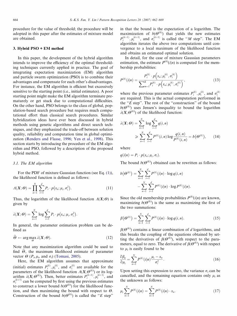
This procedure for adjusting the 3N particles involvesselection of the global best particle and finally velocityupdates. The global best particle of the population is deter-mined according to the sorted fitness values. Note that ifthe global best particle could not be updated through theEM algorithm, the PSO + EM algorithm will generate anew one to replace the old one, and reselect the global bestparticle in the new swarm. So, selection (or called filtering)in PSO + EM is possible. By Eqs. (21) and (22), a velocityupdate for each of 3N particles is then carried out. The3N + 1 particles are sorted in preparation for repeatingthe next iteration. The process terminates when a certainconvergence criterion is satisfied. Here, Fig. 1 summarizesthe procedure of PSO + EM and Fig. 2 shows theflowchart.

4. Experimental results

In this section, we evaluate and compare the perfor-mances of these two methods: the NM-PSO algorithmand proposed PSO + EM algorithm while implementingGaussian curve fitting for multi-level thresholding. Bothmethods are implemented on an Intel Celeron 2.8 GHzplatform with 512 MB DDR-RAM using Matlab. The testimages are of size 256 · 256 pixels with 8 bit gray-levels,taken under natural room lighting without the supportof any special light source. The stopping criterion ofNM-PSO referred to Zahara et al. (2005) is 10N iterationswhen solving an N-dimensional problem. However, the

Generate PSO population

of size 3N+1

Evaluate the fitnessof each particle

Rank particles based on the fitness

Apply EM approach to update

the best particle once

Updated successfully?

Generate a new solution randomly.

Does likelihoodconverge?

Apply velocity update to the remaining 3N

particles

Gain the optimumsolution (estimates)

Fitness function

Compute likelihood of updated solution

No

Yes

Yes

No

Fig. 2. Flowchart of PSO + EM algorithm.

Fig. 3. Experimental resul

666 S.-K.S. Fan, Y. Lin / Pattern Recognition Letters 28 (2007) 662–669

PSO + EM algorithm is halted while the likelihood func-tion improvement falls within 10�6. To fairly comparethese two parametric methods’ efficiency and effectiveness,for the NM-PSO algorithm the initial parameter estimatesused in (Zahara et al., 2005) are followed. For thePSO + EM algorithm, the prior estimates, P 0is, are set atPi = 1/d; remaining parameters are all generated atrandom.

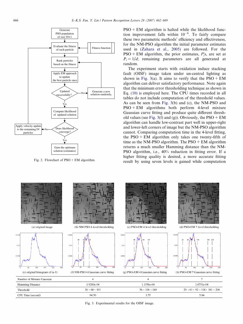
The experiment starts with oxidation induce stackingfault (OISF) image taken under un-central lighting asshown in Fig. 3(a). It aims to verify that the PSO + EMalgorithm can deliver satisfactory performance. Note againthat the minimum error thresholding technique as shown inEq. (10) is employed here. The CPU times recorded in alltables do not include computation of the threshold values.As can be seen from Fig. 3(b) and (c), the NM-PSO andPSO + EM algorithms both perform 4-level mixtureGaussian curve fitting and produce quite different thresh-old values (see Fig. 3(f) and (g)). Obviously, the PSO + EMalgorithm can handle low-contrast part well in upper-rightand lower-left corners of image but the NM-PSO algorithmcannot. Comparing computation time in the 4-level fitting,the PSO + EM algorithm only takes one twenty-fifth oftime as the NM-PSO algorithm. The PSO + EM algorithmreturns a much smaller Hamming distance than the NM-PSO algorithm, i.e., 40% reduction in fitting error. If ahigher fitting quality is desired, a more accurate fittingresult by using seven levels is gained while computation

ts for the OISF image.

S.-K.S. Fan, Y. Lin / Pattern Recognition Letters 28 (2007) 662–669 667

time increases only to 5.84 s from 3.75 s. To be precise, thefurther improvement on Hamming distance made from 4-to 7-level fitting is about 5%.

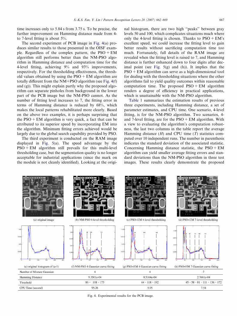
The second experiment of PCB image in Fig. 4(a) pro-duces similar results to those presented in the OISF exam-ple. Regardless of the complex pattern, the PSO + EMalgorithm still performs better than the NM-PSO algo-rithm in Hamming distance and computation time for the4-level fitting, achieving 9% and 93% improvements,respectively. For the thresholding effectiveness, the thresh-old values obtained by using the PSO + EM algorithm aretotally different from the NM+PSO algorithm (see Fig. 4(f)and (g)). This might explain partly why the proposed algo-rithm can separate pinholes from background in the lowerpart of the PCB image but the NM-PSO cannot. As thenumber of fitting level increases to 7, the fitting error interms of Hamming distance is reduced by 68%, whichmakes the local patterns rehabilitated more clearly. Basedon the above two examples, it is perhaps surprising thatthe PSO + EM algorithm is very quick, a fact that can beattributed to its superior speed by incorporating EM intothe algorithm. Minimum fitting errors achieved would belargely due to the global search capability provided by PSO.

The third experiment is conducted on the RAM imagedisplayed in Fig. 5(a). The speed advantage by thePSO + EM algorithm still prevails for this multi-levelthresholding case, but the segmentation quality is no longeracceptable for industrial applications (since the mark onthe module is not cleanly identified). Looking at the origi-

Fig. 4. Experimental resul

nal histogram, there are two high ‘‘peaks’’ between graylevels 50 and 100, which complicates situations much whereonly the 4-level fitting is chosen. Thanks to PSO + EM’sexcellent speed, we could increase the fitting level to gainbetter results without sacrificing computation time toomuch. Fortunately, full details of the RAM image arerevealed when the fitting level is raised to 7, and Hammingdistance is further enhanced down to four digits after dec-imal point (see Fig. 5(g) and (h)). It implies that thePSO + EM algorithm can serve as a high-dimensional toolfor dealing with the thresholding situations where the otheralgorithms fail to yield quality outcomes within reasonablecomputation time. The proposed PSO + EM algorithmrenders a degree of efficiency in practical applications,which is unattainable with the NM-PSO algorithm.

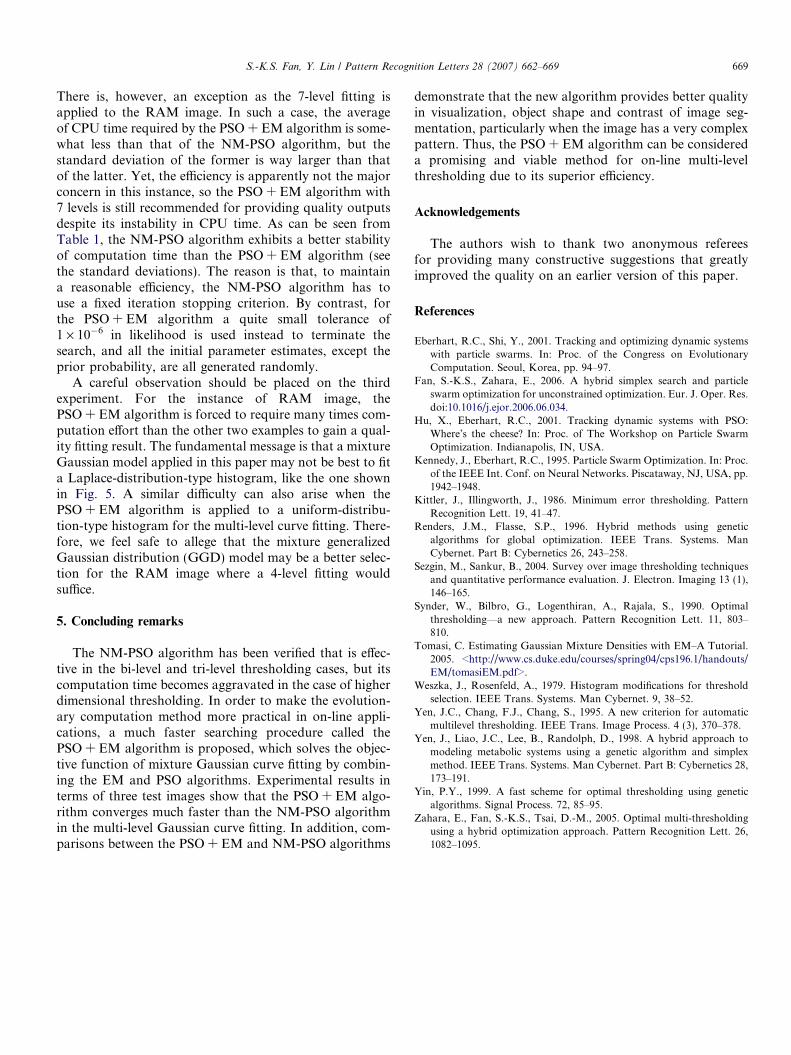
Table 1 summarizes the estimation results of previousthree experiments, including Hamming distance, a set ofparameter estimates, and CPU time. One scenario, 4-levelfitting, is for the NM-PSO algorithm. Two scenarios, 4-and 7-level fitting, are for the PSO + EM algorithm. Witha view to evaluating the algorithm’s computation robust-ness, the last two columns in the table report the averageHamming distance (H) and CPU time (T) statistics com-puted over 10 independent runs. The number in parenthesisindicates the standard deviation of the associated statistic.Concerning Hamming distance statistic, the PSO + EMalgorithm can yield smaller average fitting errors and stan-dard deviations than the NM-PSO algorithm in three testimages. These results clearly demonstrate the proposed

ts for the PCB image.

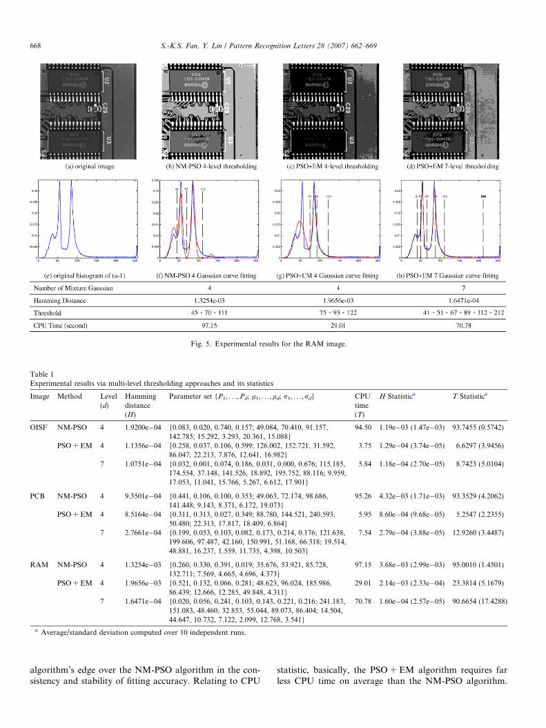
Table 1Experimental results via multi-level thresholding approaches and its statistics

Image Method Level(d)

Hammingdistance(H)

Parameter set {P1, . . .,Pd; l1, . . .,ld; r1, . . .,rd} CPUtime(T)

H Statistica T Statistica

OISF NM-PSO 4 1.9200e�04 {0.083, 0.020, 0.740, 0.157; 49.084, 70.410, 91.157,142.785; 15.292, 3.293, 20.361, 15.088}

94.50 1.19e�03 (1.47e�03) 93.7455 (0.5742)

PSO + EM 4 1.1356e�04 {0.258, 0.037, 0.106, 0.599; 126.002, 152.721, 31.592,86.047; 22.213, 7.876, 12.641, 16.982}

3.75 1.29e�04 (3.74e�05) 6.6297 (3.9456)

7 1.0751e�04 {0.032, 0.001, 0.074, 0.186, 0.031, 0.000, 0.676; 115.185,174.554, 37.148, 141.526, 18.892, 195.752, 88.116; 9.959,17.053, 11.041, 15.766, 5.267, 6.612, 17.901}

5.84 1.18e�04 (2.70e�05) 8.7423 (5.0104)

PCB NM-PSO 4 9.3501e�04 {0.441, 0.106, 0.100, 0.353; 49.063, 72.174, 98.686,141.448; 9.143, 8.371, 6.172, 19.073}

95.26 4.32e�03 (1.71e�03) 93.3529 (4.2062)

PSO + EM 4 8.5164e�04 {0.311, 0.313, 0.027, 0.349; 88.780, 144.521, 240.593,50.480; 22.313, 17.817, 18.409, 6.864}

5.95 8.60e�04 (9.68e�05) 5.2547 (2.2355)

7 2.7661e�04 {0.199, 0.053, 0.103, 0.082, 0.173, 0.214, 0.176; 121.638,199.606, 97.487, 42.160, 150.991, 51.168, 66.318; 19.514,48.881, 16.237, 1.559, 11.735, 4.398, 10.503}

7.54 2.79e�04 (3.88e�05) 12.9260 (3.4487)

RAM NM-PSO 4 1.3254e�03 {0.260, 0.330, 0.391, 0.019; 35.676, 53.921, 85.728,132.711; 7.569, 4.665, 4.696, 4.373}

97.15 3.68e�03 (2.99e�03) 95.0010 (1.4501)

PSO + EM 4 1.9656e�03 {0.521, 0.132, 0.066, 0.281; 48.623, 96.024, 185.986,86.439; 12.666, 12.285, 49.848, 4.311}

29.01 2.14e�03 (2.33e�04) 23.3814 (5.1679)

7 1.6471e�04 {0.020, 0.056, 0.241, 0.103, 0.143, 0.221, 0.216; 241.183,151.083, 48.460, 32.853, 55.044, 89.073, 86.404; 14.504,44.647, 10.732, 7.122, 2.099, 12.768, 3.541}

70.78 1.60e�04 (2.57e�05) 90.6654 (17.4288)

a Average/standard deviation computed over 10 independent runs.

Fig. 5. Experimental results for the RAM image.

668 S.-K.S. Fan, Y. Lin / Pattern Recognition Letters 28 (2007) 662–669

algorithm’s edge over the NM-PSO algorithm in the con-sistency and stability of fitting accuracy. Relating to CPU

statistic, basically, the PSO + EM algorithm requires farless CPU time on average than the NM-PSO algorithm.

S.-K.S. Fan, Y. Lin / Pattern Recognition Letters 28 (2007) 662–669 669

There is, however, an exception as the 7-level fitting isapplied to the RAM image. In such a case, the averageof CPU time required by the PSO + EM algorithm is some-what less than that of the NM-PSO algorithm, but thestandard deviation of the former is way larger than thatof the latter. Yet, the efficiency is apparently not the majorconcern in this instance, so the PSO + EM algorithm with7 levels is still recommended for providing quality outputsdespite its instability in CPU time. As can be seen fromTable 1, the NM-PSO algorithm exhibits a better stabilityof computation time than the PSO + EM algorithm (seethe standard deviations). The reason is that, to maintaina reasonable efficiency, the NM-PSO algorithm has touse a fixed iteration stopping criterion. By contrast, forthe PSO + EM algorithm a quite small tolerance of1 · 10�6 in likelihood is used instead to terminate thesearch, and all the initial parameter estimates, except theprior probability, are all generated randomly.

A careful observation should be placed on the thirdexperiment. For the instance of RAM image, thePSO + EM algorithm is forced to require many times com-putation effort than the other two examples to gain a qual-ity fitting result. The fundamental message is that a mixtureGaussian model applied in this paper may not be best to fita Laplace-distribution-type histogram, like the one shownin Fig. 5. A similar difficulty can also arise when thePSO + EM algorithm is applied to a uniform-distribu-tion-type histogram for the multi-level curve fitting. There-fore, we feel safe to allege that the mixture generalizedGaussian distribution (GGD) model may be a better selec-tion for the RAM image where a 4-level fitting wouldsuffice.

5. Concluding remarks

The NM-PSO algorithm has been verified that is effec-tive in the bi-level and tri-level thresholding cases, but itscomputation time becomes aggravated in the case of higherdimensional thresholding. In order to make the evolution-ary computation method more practical in on-line appli-cations, a much faster searching procedure called thePSO + EM algorithm is proposed, which solves the objec-tive function of mixture Gaussian curve fitting by combin-ing the EM and PSO algorithms. Experimental results interms of three test images show that the PSO + EM algo-rithm converges much faster than the NM-PSO algorithmin the multi-level Gaussian curve fitting. In addition, com-parisons between the PSO + EM and NM-PSO algorithms

demonstrate that the new algorithm provides better qualityin visualization, object shape and contrast of image seg-mentation, particularly when the image has a very complexpattern. Thus, the PSO + EM algorithm can be considereda promising and viable method for on-line multi-levelthresholding due to its superior efficiency.

Acknowledgements

The authors wish to thank two anonymous refereesfor providing many constructive suggestions that greatlyimproved the quality on an earlier version of this paper.

References

Eberhart, R.C., Shi, Y., 2001. Tracking and optimizing dynamic systemswith particle swarms. In: Proc. of the Congress on EvolutionaryComputation. Seoul, Korea, pp. 94–97.

Fan, S.-K.S., Zahara, E., 2006. A hybrid simplex search and particleswarm optimization for unconstrained optimization. Eur. J. Oper. Res.doi:10.1016/j.ejor.2006.06.034.

Hu, X., Eberhart, R.C., 2001. Tracking dynamic systems with PSO:Where’s the cheese? In: Proc. of The Workshop on Particle SwarmOptimization. Indianapolis, IN, USA.

Kennedy, J., Eberhart, R.C., 1995. Particle Swarm Optimization. In: Proc.of the IEEE Int. Conf. on Neural Networks. Piscataway, NJ, USA, pp.1942–1948.

Kittler, J., Illingworth, J., 1986. Minimum error thresholding. PatternRecognition Lett. 19, 41–47.

Renders, J.M., Flasse, S.P., 1996. Hybrid methods using geneticalgorithms for global optimization. IEEE Trans. Systems. ManCybernet. Part B: Cybernetics 26, 243–258.

Sezgin, M., Sankur, B., 2004. Survey over image thresholding techniquesand quantitative performance evaluation. J. Electron. Imaging 13 (1),146–165.

Synder, W., Bilbro, G., Logenthiran, A., Rajala, S., 1990. Optimalthresholding—a new approach. Pattern Recognition Lett. 11, 803–810.

Tomasi, C. Estimating Gaussian Mixture Densities with EM–A Tutorial.2005. <http://www.cs.duke.edu/courses/spring04/cps196.1/handouts/EM/tomasiEM.pdf>.

Weszka, J., Rosenfeld, A., 1979. Histogram modifications for thresholdselection. IEEE Trans. Systems. Man Cybernet. 9, 38–52.

Yen, J.C., Chang, F.J., Chang, S., 1995. A new criterion for automaticmultilevel thresholding. IEEE Trans. Image Process. 4 (3), 370–378.

Yen, J., Liao, J.C., Lee, B., Randolph, D., 1998. A hybrid approach tomodeling metabolic systems using a genetic algorithm and simplexmethod. IEEE Trans. Systems. Man Cybernet. Part B: Cybernetics 28,173–191.

Yin, P.Y., 1999. A fast scheme for optimal thresholding using geneticalgorithms. Signal Process. 72, 85–95.

Zahara, E., Fan, S.-K.S., Tsai, D.-M., 2005. Optimal multi-thresholdingusing a hybrid optimization approach. Pattern Recognition Lett. 26,1082–1095.