channel estimation and optimal training design for

2684 IEEE TRANSACTIONS ON WIRELESS COMMUNICATIONS, VOL. 14, NO. 5, MAY 2015

Channel Estimation and Optimal Training Designfor Correlated MIMO Two-Way Relay

Systems in Colored EnvironmentRui Wang, Member, IEEE, Meixia Tao, Senior Member, IEEE,

Hani Mehrpouyan, Member, IEEE, and Yingbo Hua, Fellow, IEEE

Abstract—In this paper, while considering the impact of the an-tenna correlation and the interference from neighboring users, weanalyze channel estimation and training sequence design for multi-input multi-output (MIMO) two-way relay systems. To this end,we propose to decompose the bidirectional transmission links intotwo phases, i.e., the multiple access (MAC) phase and the broad-cast (BC) phase. By considering the Kronecker-structured channelmodel, we derive the optimal linear minimum mean-square-error(LMMSE) channel estimators. The corresponding training designsfor the MAC phase and the BC phase are then formulated andsolved to improve channel estimation accuracy. For the generalscenario of the training sequence design for both phases, twoiterative training design algorithms are proposed that are verifiedto produce training sequences achieving near optimal channel es-timation performance. Furthermore, for specific practical scenar-ios, where the covariance matrices of the channel or disturbancesare of particular structures, the optimal training sequence designguidelines are obtained. The minimum required training lengthsfor channel estimation in both the MAC phase and the BC phaseare also analyzed. Comprehensive simulations are carried out todemonstrate the effectiveness of the proposed training designs.

Index Terms—MIMO, two-way relaying, channel estimation,linear minimum mean-square-error, convex optimization.

I. INTRODUCTION

R ELAY assisted cooperative communication has beenregarded as one of the most promising techniques in

combating long distance channel fading in complex wirelesscommunication systems. One popular example is one-way re-laying, which has been well studied in the past decade [2], [3].Although one-way relaying shows great potential in reducing

Manuscript received March 21, 2014; revised September 15, 2014 andDecember 20, 2014; accepted December 24, 2014. Date of publicationJanuary 12, 2015; date of current version May 7, 2015. The work of Rui Wangwas supported by the National Natural Science Foundation of China underGrant 61401313. The work of Meixia Tao was supported by the NSF of Chinaunder grant 61322102. Part of this work was presented at IEEE Globecom,Austin, TX, USA, December 2014. The associate editor coordinating the reviewof this paper and approving it for publication was S.Bhashyam.

R. Wang is with the College of Electronics and Information Engineering,Tongji University, Shanghai 200092, China (e-mail: [email protected]).

M. Tao is with the Department of Electronic Engineering at Shanghai JiaoTong University, Shanghai 200240, China (e-mail: [email protected]).

H. Mehrpouyan is with the Department of Computer and Electrical Engi-neering and Computer Science at California State University, Bakersfield, CA93311, USA (e-mail: [email protected]).

Y. Hua is with the University of California, Riverside, CA 92521 USA(e-mail: [email protected]).

Color versions of one or more of the figures in this paper are available onlineat http://ieeexplore.ieee.org.

Digital Object Identifier 10.1109/TWC.2015.2390645

power consumption, enhancing reliability, and extending cov-erage, it suffers from low spectral efficiency due to the half-duplex nature of the network. To overcome this disadvantage,by using the idea of network coding, two-way relaying (TWR)has been proposed and has received great attention recently. Infact, TWR can maintain the advantages of traditional relayingwhile doubling spectral efficiency.

The improvement in spectral efficiency in TWR is achievedby applying self-interference cancelation at each source nodeand extracting the desired information from the receivednetwork-coded messages. In this case, the accuracy of the self-interference cancelation process significantly affects the perfor-mance of TWR systems. Moreover, when using the popularamplify-and-forward (AF) relaying strategy, the accuracy ofself-interference cancelation process heavily depends on theprecision of the channel estimation. Thus, obtaining highlyaccurate channel state information (CSI) becomes more impor-tant in TWR systems compared to traditional one-way relayingsystems. In fact, devising new channel estimation schemesfor TWR systems has received great attention recently. Forexample, in [4], the authors propose to estimate the cascadedchannel of TWR systems under the AF relaying strategy. Byusing multiple phase shift keying (M-PSK) training symbols,blind and partially-blind channel estimators are investigated in[5], [6]. Different from [4]–[6], where flat fading channels areassumed, the authors in [7] investigate time varying channelestimation via a new complex-exponential basis expansionmodel. Moreover, in [8], [9], the channel estimation for TWRis extended to the scenario of orthogonal frequency divisionmultiplexing (OFDM) systems.

It is worth noting that the works summarized above areconcerned with single-antenna TWR systems. As expected,the multi-antenna or multi-input multi-output (MIMO) tech-nique can be introduced into TWR systems to further improvetransmission reliability and bandwidth efficiency. One efficientway to realize such performance improvement is to exploit theestimated CSI for the application of source and relay precoding[10], [11]. Therefore, in MIMO TWR systems, in additionto affecting the performance of self-interference cancelation,inaccurate channel estimation also imposes a negative effect onthe precoder design.

Fig. 1 depicts a MIMO TWR setup. Let us denote the processof data transmission from the source nodes to the relay and therelay to the source nodes as multiple access (MAC) phase and

1536-1276 © 2015 IEEE. Personal use is permitted, but republication/redistribution requires IEEE permission.See http://www.ieee.org/publications_standards/publications/rights/index.html for more information.

WANG et al.: CORRELATED MIMO TWO-WAY RELAY SYSTEMS IN COLORED ENVIRONMENT 2685

Fig. 1. An illustration of MIMO two-way relay system. (a) 1-st time slot(MAC phase); (b) 2-nd time slot (BC phase).

broadcast (BC) phase, respectively. In [12], the authors proposea MIMO channel estimator that uses the self-interference as atraining sequence to estimate the channel matrices correspond-ing to the BC phase. In [13], the performances of differentchannel estimators, including individual and cascaded channelestimators, are compared based on the least squares (LS) crite-rion. In [14], an LS estimator is used to obtain the cascadedchannel matrices corresponding to the BC and MAC phasesusing a single carrier cyclic prefix. Note that in the contributionsof [12]–[14], the channel statistics of random channel matrices,whether cascaded channels or individual channels, are assumedto be unknown. Based on the estimation theory, if channelstatistics are known, the channel estimation can be conductedunder the Bayesian framework and the estimation accuracycan be further enhanced. Hence, by taking these statistics intoaccount, we seek to improve upon the channel estimators in[12]–[14].

Very recently, the authors in [15], [16] independently in-vestigate the minimum mean-square-error (MMSE) channelestimation for TWR systems based on a correlated GaussianMIMO channel model. In particular, in [15], the cascadedchannel matrices for AF TWR systems are estimated and thetraining sequences at the two source nodes are optimized tominimize the total channel estimation MSE. Different from[15], the authors in [16] aim to estimate the individual channelmatrices for each link. To reach this goal, two different esti-mation schemes, i.e., a superimposed channel training schemeand a two-stage channel estimation scheme, are proposed. Inaddition, the training sequences at the two source nodes, as wellas, at the relay node are jointly optimized to improve channelestimation accuracy.

In this paper, similar to [1], [12]–[16], while assuming thatthe channel statistics are known, we analyze and devise channelestimators for correlated MIMO TWR systems. Specifically,we consider the Kronecker-structured channel model, such thatthe individual channel matrices can be estimated based on theBayesian framework. However, unlike [15], [16], we also takeinto account the interference from the nearby users. Thus, inthis model, the disturbance at each of the source nodes or atthe relay node consists of both noise and interference. Note thatthe considered colored estimation environment may be morepractical for applications in today’s more densely deployedwireless networks. Although channel estimation in point-to-point MIMO systems in colored environments has been studiedin [17], [18], to the best of our knowledge, this topic has notbeen addressed in the TWR scenario.

To enhance TWR performance, we seek to estimate theindividual channel matrices corresponding to the source-to-relay link and the relay-to-source link, see Fig. 1. To this end,a new two-phase estimation scheme is proposed, where thebidirectional transmission of a TWR system is decomposed intothe MAC phase and the BC phase. For the MAC and BC phases,the channel estimations are performed at the relay node andat the two source nodes, respectively. The proposed estimationscheme is different from the ones in [15], [16], where thechannel estimation is assumed to only be conducted at thesource nodes. As such, our proposed estimation scheme canmore efficiently support precoding at the relay since it requiressignificantly less feedback overhead [10], [19], [20]. Basedon the proposed estimation scheme, we derive the optimallinear MMSE (LMMSE) estimator for each phase. Next, thecorresponding training design problems are formulated with theaim of minimizing the total MSE of channel estimation processfor each phase. The training design problem considered hereis different from that of [15], [16], since we take into accountthe effect of colored disturbances caused by interference atthe relay node and at the source nodes. Moreover, the trainingdesign scenarios for point-to-point systems in [17], [18] aredifferent from the scenario under consideration in this paper,since our proposed training sequence design is optimized tosimultaneously enhance channel estimation accuracy over bothlinks in the BC phase and in the MAC phase. Although, forthe general scenario, it is difficult to derive the optimal trainingsequence structures as in [15]–[18], we propose two iterativedesign algorithms to solve the training design problems. Thesealgorithms are verified to converge quickly to the near optimalsolution and to not be sensitive to the initialization process.For some special cases, where the covariance matrices of thechannels or disturbances have specific forms, two specific ap-proaches are applied to obtain the optimal training sequences:1) the original problem is converted into a standard convexoptimization problem; 2) the optimal structures of the trainingsequences are first derived and then used to reduce the originalnon-convex problem into a simple power allocation problem.Finally, to reduce training overhead, the minimum requiredtraining lengths for channel estimation in both the MAC andBC phases are analyzed. Extensive simulations are carried outto support the findings of the paper.

The rest of the paper is organized as follows. In Section II,we present the system model. The LMMSE estimators forboth the MAC and BC phases are derived in Section III. Thetraining designs for the MAC and BC phases are analyzed inSection IV and V, respectively. Simulation results are providedin Section VI. We conclude the paper in Section VII.

Notations: E(·) denotes the expectation operator. ⊗ denotesthe Kronecker operator. vec(·) signifies the matrix vectorizationoperator. Superscripts AT , A∗, and AH denote the transpose,conjugate, and conjugate transpose of matrix A, respectively.Tr(A), A−1, det(A), and Rank(A) stand for the trace, inverse,determinant, and rank of A, respectively. λ(A) denotes a vectorcontaining eigenvalues of A. Blkdiag(A1,A2, · · · ,AN) denotesa block diagonal matrix constructed by matrices Ai, for ∀i.Diag(a) denotes a diagonal matrix with a being its diagonalentries. A(n : m, :) and A(:,n : m) denote the sub-matrices


constructed by n to m rows and n to m columns of A, respec-tively. ‖A‖2

F denotes the Frobenius norm of A. ℜ(z) denotes thereal part of a complex variable z. The distribution of a circularsymmetric complex Gaussian vector with mean vector x andcovariance matrix Σ is denoted by C N (x,Σ). Cx×y denotes thespace of complex x× y matrices. SN and S

N+ denote the set of

symmetric N ×N matrices and the set of positive semidefiniteN ×N matrices, respectively. x � y denotes that the vector ymajorizes the vector x.

II. SYSTEM MODEL

Consider a TWR system, where sources S1 and S2 exchangemessages with one another through a relay R. S1, R, and S2

are assumed to be equipped with N1, M, and N2 antennas,respectively. Channel matrices from S1 and S2 to R are denotedby H1 and H2, respectively, and channel matrices from R to S1

and S2 are denoted by G1 and G2, respectively.Signal transmission within the TWR system is achieved in

two time slots. In the first phase, referred to as the MAC phase,the source node Si, for i= 1,2, transmit their signals to the relaynode R, while in the second phase, referred to as the BC phase,the relay node R forwards its combined received signal to thetwo source nodes S1 and S2. The proposed channel estimatoraims to obtain the individual channels of the two hops, i.e.,{H1,H2,G1,G2}, which is different from the cases studiedin [4], [15] to estimate the cascaded channel. This approachfacilitates the precoding design and/or the power allocation atthe relay node, which can further improve the overall systemperformance [10], [11], [19], and [20].

Following the transmission in Fig. 1, we assume that H1 andH2 are estimated in the MAC phase via the training signalssent from the two sources, and G1 and G2 are estimated inthe BC phase via the training signal transmitted from therelay. Moreover, the channels follow quasi-static fadings, i.e.,the channel matrices {H1,H2,G1,G2} are random but stayconstant during the whole duration of transmission.

The received training signals at the relay node in the MACphase can be expressed as

yR(t) = H1s1(t)+H2s2(t)+nR(t), (1)

where si(t) denotes the training signal at Si and nR(t) repre-sents the correlated disturbance at R. nR(t) includes the totalbackground noise as well as the interference from adjacentcommunication links, and is modeled as a stochastic processwith respect to the time variable t [17], [18], [21]. To estimatethe channel matrices at the relay, the sources typically need tosend a sequence of known training signals. Assuming trainingsequences have a length of LS, the received signal in (1) can bewritten in a matrix from as

YR = H1S1 +H2S2 +NR, (2)

where YRΔ= [yR(1),yR(2), · · · ,yR(LS)], Si

Δ= [s1(1),s1(2), · · · ,

s1(LS)] and NRΔ= [nR(1),nR(2), · · · ,nR(LS)]. Suppose that the

source node Si has a maximum power of τi during the channel

estimation phase, the training sequence Si should fulfill thefollowing power constraint

Tr(SiSHi )≤ τi, i = 1,2. (3)

Now we give the distributions of the channel matrices Hi,for i = 1,2, and the disturbance NR in (2). We assume thatthe channel matrices Hi, for i = 1,2, follow the Kronecker-structured model [15]–[18], [21] and are expressed as

Hi = Cr,HWHiCTt,Hi

, i = 1,2 (4)

where indexes ‘t’ and ‘r’ denote the ‘transmitter’ and ‘receiver’,respectively; WHi , for i = 1,2, are assumed to be unknownmatrices, where their entries are modeled by C N (0,1); Cr,H

denotes the receive correlation matrix of both H1 and H2;1 andCt,Hi denotes the transmit correlation matrix of Hi. In (4), thecorrelation amongst the channel parameters can be caused byinsufficient antenna spacing as verified by the measurementsin [22], [23]. Based on the channel model in (4), we havevec(Hi)∼ C N (0,ZHi) with

ZHi = Zt,Hi ⊗Zr,H , i = 1,2, (5)

where Zt,Hi = Ct,HiCHt,Hi

and Zr,H = Cr,HCHr,H . Here, Zt,Hi , for

i = 1,2, denote the covariance matrices at the transmitter side,and Zr,H denotes the covariance matrix at the receiver side. Weassume that the correlation matrices Cr,H and Ct,Hi , for i = 1,2,are known in prior. This also implies that the channel covariancematrices Zr,H and ZHi , for i = 1,2, are known and are in turnused for the training design in the MAC phase.

Regarding the disturbance NR, we denote nR = vec(NR) andassume that nR is a random vector with mean 0 and E(nRnH

R ) =KR. Moreover, KR is structured and modeled by [17], [18]

KR = Kq,R ⊗Kr,R, (6)

where Kq,R ∈ CLS×LS denotes the temporal covariance matrix;

Kr,R ∈ CM×M denotes the receive spatial covariance matrix.

Moreover, the covariances of disturbance Kq,R and Kr,R are alsoknown in prior. This further implies that KR is known. Kq,R andKr,R shall be utilized for the training design in what follows.

In the BC phase, the received training signals at the sourcenodes are given by

yi(t) = GisR(t)+ni(t), i = 1,2 (7)

where sR(t) denotes the training signal at the relay node andni(t) represents the correlated disturbance at the source node Si.By rewriting (7) into the matrix form, we have

Yi = GiSR +Ni, i = 1,2, (8)

where YiΔ= [yi(1),yi(2), · · · ,yi(LR)], SR

Δ= [sR(1),sR(2), · · · ,

sR(LR)] and NiΔ= [ni(1),ni(2), · · · ,ni(LR) with LR being the

1Here, H1 and H2 share a common receive correlation matrix as theyterminate at the relay node.


training sequence length at the relay. The following conditionmust be met to satisfy the power constraint at the relay node

Tr(SRSHR )≤ τR. (9)

In (9), τR denotes the maximum power at the relay node duringthe training phase.

Similar to the MAC phase, the channel matrices in the BCphase also follow the Kronecker-structured model, i.e.,

Gi = Cr,GiWGi CTt,G, i = 1,2, (10)

where WGi , for i = 1,2, are unknown matrices in which theentries are modeled by C N (0,1); Ct,G denotes the transmitcorrelation matrix of both G1 and G2;2 and Cr,Gi denotesthe receive correlation matrix of Gi. We also assume that thecorrelation matrices Ct,G and Cr,Gi , for i = 1,2, are known inprior and will be used for the training sequence design in theBC phase. Based on (10), we then have vec(Gi)∼ C N (0,ZGi)with

ZGi = Zt,G ⊗Zr,Gi , i = 1,2, (11)

where Zt,G = Ct,GCHt,G and Zr,Gi = Cr,GiC

Hr,Gi

.As in (6), we denote ni = vec(Ni), for i = 1,2, and assume

that ni is a random vector with mean 0 and E(ninHi ) = Ki with

Ki having a structure of

Ki = Kq,i ⊗Kr,i ∈ SNiLR×NiLR , i = 1,2, (12)

where Kq,i ∈ CLR×LR , for i = 1,2, denote the temporal covari-

ance matrices and Kr,i ∈CNi×Ni , for i= 1,2, denote the received

spatial covariance matrices. Also, we assume that the statisticsof Kq,i and Kr,i, for i = 1,2, are known in prior.

Other assumptions made throughout this paper are listedas follows. We assume that Kr,1, Kr,2, and Kr,R share thesame eigenvectors with Zr,G1 , Zr,G2 and Zr,H , respectively. Thisassumption models the following scenarios as summarized in[18], [21]: 1) Additive noise-limited scenario, KR = µRIMLS =ILS ⊗ µRIM and Ki = µiINiLR = ILR ⊗ µiINi , for i = 1,2, whichimplies Kr,R = µRIM and Kr,i = µiINi with µR and µi being thevariances of the additive noises at the relay and the sourcesSi, respectively; 2) Interference-limited scenario, KR = QR ⊗Zr,H , Ki = QGi ⊗ Zr,Gi with QR and QGi , i = 1,2, denotingthe temporal covariances from nearby interfering users, whichimplies Kr,R = Zr,H and Kr,i = Zr,Gi , for i = 1,2; 3) Addi-tive noise and temporally uncorrelated interference scenario,KR = µRIMLS +νRILS ⊗Zr,H = ILS ⊗(µRIM +νRZr,H) and Ki =µiINiLR + νiILR ⊗Zr,Gi = ILR ⊗ (µiINi + νiZr,Gi), which impliesKr,R = µRIM + νRZr,H and Kr,i = µiINi + νiZr,Gi , for i = 1,2,with νR and νi being the powers of the interfering users at therelay and at the source Si, respectively, µR and µi being thevariances of the additive noises at the relay and at the source Si,respectively; 4) Additive noise and spatially uncorrelated inter-ference scenario, KR = µRIMLS +QR⊗IM = (µRILS +QR)⊗IM ,Ki = µiINiLR +QGi ⊗ INi = (µiILR +QGi)⊗ INi , which impliesKr,R = IM and Kr,i = INi , for i = 1,2.

2Here, G1 and G2 share a common transmit correlation matrix as they beginat the relay node.

For ease of the following training designs, we give thefollowing definitions. The eigenvalue decomposition (EVD) ofZt,Hi , Zr,H , Zt,G, and Zr,Gi are given by

Za,b = Ua,bΣa,bUHa,b, (13)

where a ∈ {r, t}, b ∈ {H,H1,H2,G,G1,G2}, Ua,b denotes theunitary eigenvector matrix and Σa,b is a diagonal matrix with[Σa,b]n,n = σa,b,n being the n-th eigenvalue of Za,b. Accordingly,the singular value decomposition (SVD) of Ca,b is denoted by

Ca,b = Ua,bΣ1/2a,b UH

a,b with Ua,b representing a unitary matrix.The EVD of Kq,i and Kr,i is denoted by

Ka,b = Va,bΔa,bVHa,b, a ∈ {r, t},b ∈ {1,2,R}, (14)

where Va,b denotes the unitary eigenvector matrix, Δa,b is adiagonal matrix with [Δa,b]n,n = δa,b,n being the n-th eigenvalueof Ka,b. As mentioned before, it is assumed that Vr,1 = Ur,G1 ,Vr,2 = Ur,G2 and Vr,R = Ur,H .

III. CHANNEL ESTIMATION FOR

TWO-WAY RELAY SYSTEMS

Following the proposed estimation scheme in Section II, wenext obtain the channel estimates based on (2) and (8). For theestimation during the MAC phase, we rewrite (2) as

YR =Cr,HWH1 CTt,H1

S1 +Cr,HWH2CTt,H2

S2 +NR

=Cr,HWHCTt,HS+NR, (15)

where WHΔ= [WH1 ,WH2 ], Ct,H

Δ= Blkdiag(Ct,H1 ,Ct,H2), and

S Δ= [ST

1 ,ST2 ]

T . Vectorizing YR in (15) and applying the identity

vec(ABC) = (CT ⊗A)vec(B), (16)

we can rewrite (15) into

yR =(ST Ct,H ⊗Cr,H

)wH +nR, (17)

where yRΔ= vec(YR) and wH

Δ= vec(WH). The estimation of wH

based on the LMMSE criterion can be obtained as wH = TRyR.The estimation matrix TR has the following form [24]

TR = ℜwhyR ℜ−1yRyR

. (18)

where ℜwhyR

Δ=E(wHyH

R )=CHt,HS∗⊗CH

r,H , ℜyRyR

Δ=E(yRyH

R ) =

(ST Ct,H ⊗ Cr,H)(ST Ct,H ⊗ Cr,H)H + KR = ST Ct,HCH

t,HS∗ ⊗Cr,HCH

r,H +KR. With H Δ= [H1,H2], we define h Δ

= vec(H) =(Ct,H ⊗Cr,H)wH where Cr,H and Ct,H are defined in (4) and(15), respectively.

Then, the resulting estimation error, or mean-square-error(MSE), eR can be derived as

eR =E(‖h− h‖2

2

)=E

(Tr

[C0,H(wH − wH)(wH − wH)

H])=E

(Tr

[C0,H(wH −TRyR)(wH −TRyR)

H]) , (19)


where C0,HΔ= CH

t,HCt,H ⊗CHr,HCr,H . Substituting TR into (19)

and using the rule (I+AB)−1 = I−A(I+BA)−1B, we obtainthe following more compact form for eR

eR = Tr[C0,H

(I+

(ST Ct,H ⊗Cr,H

)HK−1

R

×(ST Ct,H ⊗Cr,H

))−1]. (20)

During the BC phase, the channel estimation should be basedon the received signal in (8). By vectorizing Yi in (8), we have

yi =(ST

RCt,G ⊗Cr,Gi

)wGi +ni, i = 1,2 (21)

where yiΔ= vec(Yi) and wGi

Δ= vec(WGi). Similar to steps

above, the estimation MSE of gi with giΔ= vec(Gi) can be

obtained as

ei =E(‖gi − gi‖2

2

)=E

(Tr

[C0,Gi(wGi − wGi)(wGi − wGi)

H])=E

(Tr

[C0,Gi(wH −Tiyi)(wH −Tiyi)

H]) , (22)

where C0,Gi

Δ= CH

t,GCt,G ⊗CHr,Gi

Cr,Gi and

Ti = ℜwGi yiℜ−1yiyi

, i = 1,2. (23)

In (23), ℜwGi yi = E(wGiyiH) = CHt,GS∗

R ⊗ CHr,Gi

, ℜyiyi =

E(yiyHi ) = (ST

i Ct,G ⊗ Cr,Gi)(STRCt,G ⊗ Cr,Gi)

H + Ki =ST

RCt,GCHt,GS∗

R ⊗Cr,GiCHr,Gi

+Ki. By substituting Ti into (22),we obtain

ei = Tr[C0,Gi

(I+

(ST

RCt,G ⊗Cr,Gi

)HK−1

i

×(ST

RCt,G ⊗Cr,Gi

))−1]. (24)

IV. TRAINING SEQUENCE DESIGN FOR MAC PHASE

In this section, the design of the training sequences for theMAC phase is analyzed. Namely, we shall optimize the trainingsequences S1 and S2 subject to two source power constraintsto minimize the total estimation MSE, i.e., eR in (19). Thecorresponding training sequence optimization problem can beformulated as

minS1,S2

eR in (19)

s.t. Tr(SiSHi )≤ τi, i = 1,2. (25)

Before solving (25), we first introduce the following lemmathat deals with the minimum length of S, LS.

Lemma 1: For an arbitrary Kq,R, for the total MSE to tendto zero as the power at each of source tends to infinity, theminimum length of the source training sequence must be LS =N1+N2. Otherwise, when LS < N1+N2, the total MSE is lowerbounded by ∑M

n=1 σr,H,n ∑N1+N2m=LS+1 σt,H,m, where σt,H,n is the

n-th element of λ(Zr,H) with Zt,H =Blkdiag(Zt,H1 ,Zt,H2) as thepower at each of source tends to infinity.

For Kq,R = qI and with finite power at the source nodes, theminimum length of the training sequences transmitted from thesource nodes must be r ≤ N1 +N2. It is important to note thatr denotes the rank of the optimal solution of S ∈ C

(N1+N2)×LS ,where LS is an arbitrary integer satisfying LS ≥N1+N2 in (25).3

Proof: See Appendix A.Next, we seek to solve the non-convex optimization problem

in (25) with respect to S1 and S2. Although the objectivefunction in (25) has a similar form to that of point-to-pointsystems, there are two power constraints in (25) that make theproblem of solving this non-convex optimization problem moredifficult than that of point-to-point systems in [17] and [18].To proceed, we first note that eR in (20) can be obtained bysubstituting (18) into (19). Thus, to make the problem tractable,we propose an iterative algorithm, which decouples the primalproblem into two sub-problems such that we can solve eachof them in an alternating manner. Let us rewrite (20) into thefollowing form

eR =E(Tr

[C0,H(wH −TRyR)(wH −TRyR)

H])=Tr

[C0,H −

(ST Ct,H ⊗Cr,H

)HTH

R CH0,H −C0,HTR

×(ST Ct,H ⊗Cr,H)+C0,HTR

(ST Ct,H ⊗Cr,H

)×(ST Ct,H ⊗Cr,H

)HTH

R +C0,HTRKRTHR

]. (26)

Then, the optimization problem in (25) is equivalent to

minTR,S1,S2

eR in (26)

s.t. Tr(SiSHi )≤ τi, i = 1,2. (27)

In the first subproblem, we intend to optimize the LMMSEestimator matrix TR for a given S1 and S2. Since TR is notrelated to the the power constraint, the problem simplifies toan unconstrained optimization problem given by

minTR

eR in (26). (28)

Given that (28) is convex with respect to TR, the optimal TR canbe obtained as given in (18).

In the second subproblem, the training sequences S1 and S2

need to be optimized for a given TR by solving the followingoptimization problem

minS1,S2

eR in (26)

s.t.q Tr(SiSHi )≤ τi, i = 1,2. (29)

We next show that the optimization problem in (29) can betransformed into a convex quadratically constrained quadratic

3We note that for an arbitrary Kq,R without a form of qI, it is difficult toderive the minimum length of the training sequence with finite source powersas it highly depends on the structure of Kq,R.


programable (QCQP) problem [25]. To achieve this goal, wefirst reformulate the last term in (26) as

Tr[C0,HTR

(ST Ct,H ⊗Cr,H

)(ST Ct,H ⊗Cr,H

)HTH

R

](a)= Tr

[TH

R C0,HTR(ST ⊗ IM)

×(Ct,HCHt,H ⊗Cr,HCH

r,H)(S∗ ⊗ IM)

](b)= vec(S⊗ IM)H (

THR C0,HTR ⊗CT

tr

)vec(S⊗ IM)

(c)= sHEH (

THR C0,HTR ⊗CT

tr

)Es, (30)

where CtrΔ=Ct,HCH

t,H⊗Cr,HCHr,H , s Δ

=vec(S), E Δ=Blkdiag(E(1),

E(2), · · · , E(LS)), E(i) = E, E Δ= [E(1); E(2); · · · ; E(M)], E(i)

Δ=

Blkdiag( ei,ei, · · · ,ei︸︷︷︸N1+N2 elements

), and eiΔ= [0,0, · · · , 1︸︷︷︸

i−th element

, · · · ,0]T .

In (30), Eq. (a) is obtained by using the circular propertyTr{AB}= Tr{BA} and the matrix identity

(A⊗B)(C⊗D) = AC⊗BD, (31)

Eq. (b) is obtained by using the identity Tr(ABCD) =vec(D)T (A⊗CT )vec(BT ) and (A⊗B)H = AH ⊗BH , and Eq.(c) is obtained by using vec(S⊗ IM) = Es. Similarly, the termTr[C0,HTR(ST Ct,H ⊗Cr,H)] can be expressed as

Tr[C0,HTR(ST Ct,H ⊗Cr,H)

]= Tr

[(S⊗ IM)T (Ct,H ⊗Cr,H)C0,HTR

]= vec(S⊗ IM)T vec(CT )

= vec(CT )T Es, (32)

where CTΔ= (Ct,H ⊗Cr,H)C0,HTR. To obtain (32), we use

Tr(AT B) = vec(A)T vec(B). (33)

The source power constraint in (29) can be rewritten as

Tr(SiSHi ) = Tr(EiSSH), (34)

where E1Δ=Blkdiag(IN1,0N2×N2) and E2

Δ=Blkdiag(0N1×N1 ,IN2).

Based on the property that Tr(ABCD) = vec(DT )T (CT ⊗A)vec(B), (34) can be further modified as

Tr(SiSHi ) = sH(I⊗Ei)s. (35)

According to (30), (32), and (35), the optimization problem in(29) can be transformed into

mins

sHEH (TH

R C0,HTR ⊗CTtr

)Es−2ℜ(vec(CT )

T Es)

s.t. sH(I⊗Ei)s ≤ τi, i = 1,2. (36)

Since both EH(THR TR ⊗CT

tr)E and I⊗Ei are positive semidefi-nite matrices, we conclude that the optimization problem in (36)is a convex QCQP problem, which can be easily solved by ap-

plying the available software package. In summary, we outlinethe proposed iterative training design algorithm as follows:

Algorithm 1

• Initialize S1, S2

• Repeat

— Update the LMMSE estimator matrix TR using (18)for fixed S1 and S2;

— For a fixed TR, solve the convex QCQP problem in(36) to get the optimal S1 and S2;

• Until The difference between the MSE from one itera-tion to another is smaller than a certain predeterminedthreshold.

Theorem 1: The proposed iterative precoding design inAlgorithm 1 is convergent and the limit point of the iterationis a stationary point of (27).

Proof: We first prove that Algorithm 1 is convergent. Tothis end, we show that the sequence of the updates of thevalue of the objective function in (27) is convergent. Let usdenote the value of the objective function in (27) by MSE

and define S Δ= [ST

1 ,ST2 ]

T as in (15). We also denote T(n)R and

S(n) as the n-th updates of TR and S, respectively. MSE(2n−1)

is used to represent the value of the (2n − 1)-th update of

MSE when TR = T(n)R and S = S(n−1). Similarly, MSE(2n)

indicates the value of the 2n-th update of MSE when TR = T(n)R

and S = S(n). Consider that the solutions of TR and S fromsubproblems (28) and (29), respectively, are optimal. For eachupdate of TR or S, the value of MSE always decreases, i.e.,MSE(n) ≤ MSE(n−1). This further indicates that the sequence{MSE(n)}∞

n=1 decreases monotonically. Moreover, as the valueof MSE is lower bounded (at least by zero), it can be concludedthat the sequence {MSE(n)}∞

n=1 is convergent based on themonotone convergence theorem in [26], i.e., for an arbitraryε, we can always find an N such that |MSE(n)−MSE(m)| ≤ εwhen n > m ≥ N.

Now we prove the convergence of the sequences {T(n)R }∞

n=1and {S(n)}∞

n=1. We first prove the convergence of {S(n)}∞n=1

by showing limn→∞ S(n) − S(n−1) = X(n) = 0 using acontradiction. Assume X(n) �= 0 with n → ∞, we then have|MSE(2n−1)−MSE(2n)|= |Tr[(X(n)T Ct,H ⊗Cr,H)

HT(n)HR CH

0,H +

C0,HT(n)R (X(n)T Ct,H ⊗ Cr,H) + C0,HT(n)

R (S(n)T Zt,HS(n)∗ ⊗Zr,H)T

(n)HR − C0,HT(n)

R (S(n−1)T Zt,HS(n−1)∗ ⊗ Zr,H)T(n)HR ]|,

which can not approach zero even as n → ∞. This contradictsthe result that the sequence {MSE(n)}∞

n=1 is convergent. Thisimplies that the sequence {S(n)}∞

n=1 is convergent. Repeatingthe same argument, we can also prove the convergence of

the sequence {T(n)R }∞

n=1. As a convergent sequence alwayshas a unique limit point, we, thus, obtain that the sequences

{T(n)R }∞

n=1 and {S(n)}∞n=1 always have limit points, which are

denoted by TR and S = [ST1 , S

T2 ]

T , respectively.


We now prove that the limit point is a stationary point of(27). To proceed, we denote Y = {TR, S1, S2}. Since at thelimit point Y, TR is the local minimizer of subproblem (28),which implies that TR satisfies the following Karush-Kuhn-Tucker (KKT) condition [25]

∂eR(S1, S2)

∂TR|TR=TR

= 0, (37)

where eR(S1, S2) denotes the function eR with S1 and S2 beingevaluated at S1 and S2, respectively. Similarly, Si, for i = 1,2,is the local minimizer of subproblem (29), which satisfies thefollowing KKT conditions

∂eR(TR)

∂Si|Si=Si

=0,

λi(Tr(SiSH

i )− τi)=0, i = 1,2 (38)

where λi is the Lagrangian multiplier associated with the sourcepower constraints. By summing up the KKT conditions givenin (37) and (38), it can be concluded that the limit point Ysatisfies the KKT conditions of the primal problem in (27),which further means that Y is a stationary point of (27).

To this point, it is shown that the joint source training designcan be solved via Algorithm 1. In the following, we illustratethat for some special cases, the optimal solution of (25) can beobtained in closed-form.

A. When Kr,R = Zr,H

We first consider the case with Kr,R = Zr,H . This case isapplicable in the scenario where the disturbance is dominatedby the interference from neighboring users as shown in [21].Accordingly, the LMMSE estimator given in (18) can be rewrit-ten as

TR =[CH

t,HS∗ ⊗CHr,H

]×[ST Ct,HCH

t,HS∗ ⊗Cr,HCHr,H +KR

]−1

(a)=

[CH

t,HS∗ ⊗CHr,H

]×[(

ST Ct,HCHt,HS∗+Kq,R

)−1 ⊗Z−1r,H

]=TR,1 ⊗C−1

r,H , (39)

where TR,1 = CHt,HS∗(ST Ct,HCH

t,HS∗ +Kq,R)−1 and in obtain-

ing Eq. (a), we have used the fact KR = Kq,R ⊗ Kr,R =Kq,R ⊗ Zr,H . The new form of TR in (39) further leadsto TH

R C0,HTR = (TR,1 ⊗C−1r,H)

H(CHt,HCt,H ⊗CH

r,HCr,H)(TR,1 ⊗C−1

r,H) = THR,1CH

t,HCt,HTR,1 ⊗ IM , and

Tr[C0,HTR

(ST Ct,H ⊗Cr,H

)(ST Ct,H ⊗Cr,H

)HTH

R

]= Tr

[(ST Ct,HCH

t,HS∗ ⊗Cr,HCHr,H

)×

(TH

R,1CHt,HCt,HTR,1 ⊗ IM

)](a)= Tr(Zr,H)Tr

[ST Ct,HCH

t,HS∗THR,1CH

t,HCt,HTR,1]

(b)= Tr(Zr,H)

2

∑i=1

Tr(ST

i Zt,HiS∗i TH

R,1CHt,HCt,HTR,1

). (40)

In (40), Eq. (a) is obtained with Tr(A ⊗ B) = Tr(A)Tr(B),and Eq. (b) is derived based on the fact that Ct,H is ablock diagonal matrix as shown in (15). In addition, the termTr[C0,HTR(ST Ct,H ⊗Cr,H)] can be reexpressed as

Tr[C0,HTR(ST Ct,H ⊗Cr,H)

]= Tr

[(ST Ct,HCH

t,HCt,HTR,1)⊗Cr,HCHr,H

]= Tr(Zr,H)

2

∑i=1

Tr(ST

i Zt,HiCt,HiTR,1,i), (41)

where TR,1,1Δ= TR,1(1 : N1, :) and TR,1,2

Δ= TR,1(N1 + 1 : N1 +

N2, :). Based on (40) and (41), (29) is equivalent to the follow-ing optimization problem

minS1,S2

2

∑i=1

{Tr

(ST

i Zt,HiS∗i TH

R,1CHt,HCt,HTR,1

)−Tr

(ST

i Zt,HiCt,HiTR,1,i)

−Tr(TH

R,1,iCHt,Hi

ZHt,Hi

S∗i

)}s.t. Tr(SiSH

i )≤ τi, i = 1,2. (42)

Although the optimization in (42) is convex and can be con-verted to a convex QCQP problem similar to (36). A closerinvestigation shows that the optimization problem in (42) canbe more easily solved compared to (29). This follows from thefact that the training matrices S1 and S2 are fully decoupled inthe objective function. As shown below, this specific conditionof the optimization in (42) allows us to find a closed-formsolution for this problem via the KKT conditions. Such aapproach significantly reduces the complexity of solving thisoptimization problem compared to using the QCQP approach.

The Lagrangian function of (42) is first derived as

L =2

∑i=1

{Tr

(ST

i Zt,HiS∗i TH

R,1CHt,HCt,HTR,1

)−Tr

(ST

i Zt,HiCt,HiTR,1,i)−Tr

(TH

R,1,iCHt,Hi

ZHt,Hi

S∗i

)}+

2

∑i=1

λi[Tr(SiSH

i )− τi],

where λi is the Lagrangian multiplier associated with the powerconstraint at the source Si. The KKT conditions for (42) can bederived as follows [25]

∂L∂Si

∗ =(TH

R,1CHt,HCt,HTR,1ST

i Zt,Hi

)T

−(TH

R,1,iCHt,Hi

ZHt,Hi

)T+λiSi = 0, (43a)

λi[Tr(SiSH

i )− τi]= 0, (43b)

Tr(SiSHi )≤ τi, i = 1,2. (43c)

Based on the KKT conditions shown in (43a) and by using (16),

the optimal siΔ= vec(Si) can be obtained as

si = [Xs,1 ⊗Xs,2,i +λiI]−1 xs,3,i, (44)


where Xs,1Δ= TH

R,1CHt,HCt,HTR,1, Xs,2,i

Δ= ZT

t,Hi, and xs,3,i

Δ=

vec((THR,1,iC

Ht,Hi

ZHt,Hi

)T ). The optimal λi in (44) can be zero orshould be chosen to activate the power constraint in (43c). Forthe case where λi �= 0, the following lemma is introduced.

Lemma 2: The function g(λi) = Tr{SiSHi }= Tr{sisH

i }, withsi defined above (44), monotonically decreases with respect to

λi and the optimal λi is upper bounded by√

σs,3,iτi

− σs,min,i.

Here, σs,min,i denotes the smallest eigenvalue of Xs,1⊗Xs,2,i andσs,3,i = ‖xs,3,i‖2

2.Proof: See Appendix B. �

By applying Lemma 2, the optimal λi that meets the con-dition Tr{SiSH

i } = τi can be readily obtained via the bisectionsearch algorithm.

B. When Kq,R = qIM

This scenario corresponds to the practical case, where thedisturbance consists of both the additive white Gaussian noiseand the temporally uncorrelated interference. Similar to thederivations in Appendix A, the total MSE can be derived as

eR =Tr

[C0,H

(IM(N1+N2) +

(ST Ct,H ⊗Cr,H

)HK−1

R

×(ST Ct,H ⊗Cr,H

))−1]

=Tr

[C0,H

(IM(N1+N2) +

1q

CHt,HS∗ST Ct,H

⊗ CHr,HK−1

r,R Cr,H

)−1]

=M

∑n=1

σr,H,nTr

[(Z−1

t,H +αnS∗ST)−1

],

where αn =σr,H,nqδr,R,n

. Subsequently, the optimization problem in(25) can be rewritten as

minS1,S2

M

∑n=1

σr,H,nTr

[(Z−1

t,H +αnS∗ST)−1

]

s.t. Tr(EiS∗ST )≤ τi, i = 1,2 (45)

where Ei is defined in (34). Although the optimization problemin (45) is non-convex with respect to Si, it is noted that onemay optimize (45) with respect to the positive semidefinitematrix S∗ST instead of the training sequence Si. This approachis preferable since in (45), the objective function and theconstraint both depend on S∗ST and not Si. Hence, by defining

QSΔ= S∗ST , the following equivalent problem can be obtained

minQS�0

M

∑n=1

σr,H,nTr

[(Z−1

t,H +αnQS

)−1]

s.t. Tr(EiQS)≤ τi, i = 1,2. (46)

Note that although the mapping from S to QS is a many-to-onemapping, the optimal value of the objective function in (46)is equal to the one in (45). Based on this fact, if we find the

optimal solution of (46), which is denoted as QS, we can alwaysobtain an SS with QS = S∗ST , which is also the optimal solutionof (45).

Theorem 2: The optimization problem in (46) is convex withrespect to the positive semidefinite matrix QS.

Proof: See Appendix C. �Next, we further show that the optimization problem in (46)

can be solved by transforming it into a semidefinite program-ming (SDP) problem. By introducing the variables Xn for n =1,2, · · · ,M, the problem in (46) can be rewritten in an equivalentform as

minQS�0,Xn

M

∑n=1

σr,H,nTr(Xn)

s.t. Tr(EiQS)≤ τi, i = 1,2(Z−1

t,H +αnQS

)−1 Xn,∀n (47)

By using the Schur complement, (47) can be further trans-formed into the following SDP problem

minQS�0,Xn

M

∑n=1

σr,R,nTr(Xn)

s.t. Tr(EiQS)≤ τi, i = 1,2[Z−1

t,H +αnQS IN1+N2

IN1+N2 Xn

]� 0, ∀n (48)

By solving the SDP problem in (48), the optimal solution to theoptimization problem in (46) can be obtained. However, thisnumerical method of solving this optimization problem has arelatively high computational complexity. As such, to obtain theoptimal structure of Si and gain a better understanding of theoptimization in (45), the following theorem is introduced.

Theorem 3: With LS ≥ N1 + N2, the optimal training se-quence Si in (45) must satisfy the condition S∗

1ST2 = 0. In

addition, the optimal Si has a form of Si = U∗t,Hi

ΣsiVHsi

. Thecondition S∗

1ST2 = 0 can be achieved by choosing Vs1 and Vs2

such that VHs1

Vs2 = 0. Moreover, Σsi is a diagonal matrix where[Σsi ]m,m = σsi,m, and Σsi , for i = 1,2, are obtained by solving thefollowing water-filling problem

M

∑n=1

αnσr,H,nσ2t,Hi,m

(1+αnσt,Hi,mσ2si,m)

2 = λi. (49)

In (49), the optimal λi is nonnegative and should be selected tosatisfy ∑Ni

m=1 σ2si,m = τi.

Proof: See Appendix D. �Remark 1: The optimal λi in (49) can be found via

the bisection search algorithm and the optimal λi isbounded by (0,minm ∑M

n=1 αnσr,H,nσ2t,Hi,m

). The upper limitof this bound is obtained via the following relation-

ship λi = ∑Mn=1

αnσr,H,nσ2t,Hi ,m

(1+αnσt,Hi ,mσ2si ,m

)2 ≤ ∑Mn=1 αnσr,H,nσ2

t,Hi,m≤

minm ∑Mn=1 αnσr,H,nσ2

t,Hi,m.


V. TRAINING SEQUENCE DESIGN FOR BC PHASE

In this section, we intend to optimize the training sequenceSR by minimizing the total estimation MSE at the two sourceends subject to the relay power constraint. According to theMSE derived in (24), the corresponding problem can be for-mulated as

minSR

2

∑i=1

Tr[C0,Gi

(I+

(ST

RCt,G ⊗Cr,Gi

)H

×K−1i

(ST

RCt,G ⊗Cr,Gi

))−1]

s.t. Tr(SRSHR )≤ τR. (50)

It is also worth noting that the training designs for point-to-point systems in [17], [18] are not applicable to the scenariounder consideration here, since the training sequence at therelay, SR, needs to be optimized to enhance channel estimationover both links that connect the relay to the sources nodes.Prior to solving (50), let us first present the minimum trainingsequence length required for channel estimation in the BCphase.

Lemma 3: For arbitrary Kq,i, i = 1,2, for the MSE at therelay to tend to zero as the relay power tends to infinity, theminimum length of the relay training sequence must be LR =M. Otherwise, when LR < M, the total MSE is always lowerbounded by ∑M

m=LR+1 σt,G,m(∑N1n=1 σr,G1,n + ∑N2

n=1 σr,G2,n), withσt,G,m being the m-th largest eigenvalue of Zt,G as the relaypower tends to infinity.

For Kq,i = qiI, i = 1,2 and with finite power at therelay, the minimum length of the training sequence transmittedfrom the relay must be r ≤ M. It is important to note thatr denotes the optimal solution of SR ∈ C

M×LR , where LR is anarbitrary integer satisfying LR ≥ M in (50).

Proof: Since the proof is similar to the proof of Lemma 1,it is omitted for brevity. �

In general, the optimization in (50) is non-convex. Hence,as in Algorithm 1, we first propose an iterative approach tooptimize the design of the training sequence at the relay. Tothis end, the MSE, i.e., ei, given in (24) is rewritten as

ei =E(Tr

[C0,Gi(wGi −Tiyi)(wGi −Tiyi)

H])=Tr

[C0,Gi −

(ST

i Ct,G ⊗Cr,Gi

)HTH

i CH0,Gi

−C0,GiTi(ST

i Ct,G ⊗Cr,Gi

)+C0,GiTi

×(ST

i Ct,G ⊗Cr,Gi

)(ST

i Ct,G ⊗Cr,Gi

)HTH

i

+C0,GiTiKiTHi

]. (51)

Since (22) and (24) are in equivalent form, the optimizationproblem in (50) can be rewritten as

minT1,T2,SR

e1 + e2

s.t. Tr(SRSHR )≤ τR. (52)

In the first subproblem, for a given SR, the optimal LMMSEestimators T1 and T2 at the two source ends are obtained asgiven in (23). Thus, we focus on solving the second subprob-lem, where the relay training sequence is optimized for a fixed

LMMSE estimator. Similar to (30) and (32), the MSE in (51) isreexpressed as

ei =sHR EH

i

(TH

i C0,GiTi ⊗CTtr,Gi

)EisR

−vec(CT,Gi)T EisR −vec(C∗

T,Gi)T Eis∗R

+Tr(C0,GiTiKiTHi )+Tr(C0,Gi),

where sRΔ= vec(SR), Ctr,Gi

Δ= Ct,GCH

t,G ⊗ Cr,GiCHr,Gi

, and

CT,Gi

Δ= (Ct,G⊗Cr,Gi)C0,GiTi. In this case, Ei is an NiLR×MLR

matrix that is constructed as in (30). Accordingly, (52) can berewritten as

minSR

sHR ARsR −aT

RsR −aHR s∗R

s.t. sHR sR ≤ τR, (53)

where ARΔ= ∑2

i=1 EHi (T

Hi C0,GiTi ⊗ CT

tr,Gi)Ei and aR

Δ=

ET1 vec(CT,G1) + ET

2 vec(CT,G2). Note that different from thesource training design, (53) has only one power constraint.Thus, its solution can be obtained via the KKT conditionsgiven by

ARsR −a∗R +λsR =0,λ(sH

R sR − τR) =0,

sHR sR − τR ≤0, (54)

where λ is the Lagrangian multiplier associated with the relaypower constraint. The solution of (53) is obtained as

sR = (AR +λI)−1a∗R. (55)

In (55), if the solution sR with λ = 0 violates the KKTconditions given in (54), λ should be chosen to meet sH

R sR = τR.Consequently, we introduce the following lemma.

Lemma 4: The function g(λ) = sHR sR, with sR defined in

(55), monotonically decreases with respect to λ. Moreover, the

optimal λ is upper-bounded by√

σa,RτR

−σR,min with σa,R = aTRa∗R

and σR,min denoting the smallest eigenvalue of AR.Proof: Since the proof is similar to that of Lemma 2, it is

omitted for brevity.Using the above steps, the overall relay training design

algorithm can be summarized as follows:

Algorithm 2

• Initialize SR

• Repeat

— Update the LMMSE estimator matrix Ti, for i= 1,2,using (23) for a fixed SR;

— Update the training signal SR using (55) for a fixedTi, for i = 1,2;

• Until The difference between the MSE from one itera-tion to another is smaller than a certain predeterminedthreshold.


Note that the convergence property proven for Algorithm 1also applies to Algorithm 2. Although for the general case thesolution of SR can only be obtained via an iterative approach,it is shown that for some special cases, the optimal trainingsequence SR can be found in closed-form.

A. When Kq,i = qiI

In this subsection, we consider that the temporal covariancematrix, Kq,i, is a scalar multiple of the identity matrix. Thisscenario corresponds to the practical case, where the distur-bance consists of both the additive white Gaussian noise andthe temporally uncorrelated interference. Using similar steps asin Appendix A, we rewrite the MSE in (24) as

ei =Ni

∑n=1

σr,Gi,nTr

[(Z−1

t,G +βi,nS∗RK−1

q,i STR

)−1],

=Ni

∑n=1

σr,Gi,nTr

[(Z−1

t,G + βi,nS∗RST

R

)−1]

where βi,n =σr,Gi ,n

δr,i,nwith δr,i,n being the n-th eigenvalue of Kr,i

as defined in (14), and βi,n = βi,n/qi, for i = 1,2. Then, (50) canbe further simplified as

minSR

N1

∑n=1

σr,G1,nTr

[(Z−1

t,G + β1,nS∗RST

R

)−1]

+N2

∑n=1

σr,G2,nTr

[(Z−1

t,G + β2,nS∗RST

R

)−1]

s.t. Tr(SRSHR )≤ τR, (56)

The optimal solution of (56) is given in the following lemma.Lemma 5: The optimal SR in (56) is of the form

SR = U∗t,GΣs,RVT

s,R, (57)

where Σs,R is a positive real diagonal matrix with [Σs,R]n,n =σs,R,n, Ut,G is the eigenvector matrix of Zt,G, and Vs,R is anarbitrary unitary matrix. The eigenvalues of Zt,G correspondingto the eigenvector matrix Ut,G are arranged in the same order asthe diagonal elements of Σs,R. The optimal Σs,R can be obtainedfrom

λ =N1

∑n=1

σr,G1,nβ1,nσ2t,G,m

(1+ β1,nσt,G,mσs,R,m)2

+N1

∑n=1

σr,G2,nβ2,nσ2t,G,m

(1+ β2,nσt,G,mσs,R,m)2, (58)

where λ ∈ (0,maxm{∑N1n=1(σr,G1,nβ1,nσ2

t,G,m +

σr,G2,nβ2,nσ2t,G,m)}) can be found via the bisection search

to meet the relay’s power constraint.Proof: The expression of MSE, i.e., ei, for i = 1,2, in (56)

contains a term Tr[(Z−1t,G + βi,nS∗

RSTR)

−1]. If the eigenvalues ofZt,G and S∗

RSTR are arranged in the same order, we have [27]

λ(Z−1t,G)+λ(βi,nS∗

RSTR) � λ(Z−1

t,G + βi,nS∗RST

R). (59)

Denote by S∗RST

R = Us,RΣ2s,RUH

s,R the EVD of S∗RST

R . Sincefunction Tr(A−1) is a schur convex function with respect to theeigenvalues of A[18], based on (59), we see that the minimumvalue can be reached if Us,R = Ut,G and the eigenvalues of Zt,G,i.e., σt,G,1,σt,G,2, · · · ,σt,G,M , are arranged in the same order withdiagonal elements of Σs,R, i.e., σs,R,1,σs,R,2, · · · ,σs,R,M . Withthe structure of training sequence given in (57), the originaloptimization problem in (56) is reduced to the following powerallocation problem

minσs,R,n,∀n

N1

∑n=1

M

∑m=1

σr,G1,nσt,G,m

1+ β1,nσt,G,mσs,R,m

+N2

∑n=1

M

∑m=1

σr,G2,nσt,G,m

1+β2,nσt,G,mσs,R,m

s.t.M

∑m=1

σs,R,m ≤ τR (60)

The Lagrangian function of (60) can be written asL = ∑N1

n=1 ∑Mm=1

σr,G1,nσt,G,m

1+β1,nσt,G,mσs,R,m+∑N2

n=1 ∑Mm=1

σr,G2,nσt,G,m

1+β2,nσt,G,mσs,R,m+

λ(∑Mm=1 σs,R,m − τR), where λ is Lagrangian multiplier

associated with the power constraint given in (60). Based onthe KKT conditions, we obtain (58). Then, by setting σs,R,m = 0for ∀m, we obtain the range of λ as shown in Lemma 2.

B. When Zt,G = aI

This case corresponds to a scenario, where the relay antennasare far enough from one to another such that they are spatiallyuncorrelated. In this case, the corresponding training designproblem can be formulated as

minSR

N1

∑n=1

σr,G1,nTr

[(I+ β1,nS∗

RK−1q,1ST

R

)−1]

+N2

∑n=1

σr,G2,nTr

[(I+ β2,nS∗

RK−1q,2ST

R

)−1]

s.t. Tr(S∗RST

R)≤ τR, (61)

where σr,Gi,n = aσr,Gi,n, and βi,n = aβi,n for i = 1,2. In general,the optimization problem in (61) is non-convex with respectto SR. However, when the relay power is large enough, weapproximately use the minimum training sequence length in thecase of an infinite relay power derived in Lemma 3, i.e., LR =M.Then, (61) is equivalent to the following problem

minSR

N1

∑n=1

σr,G1,nTr

[(I+ β1,nST

RS∗RK−1

q,1

)−1]

+N2

∑n=1

σr,G2,nTr

[(I+ β2,nST

RS∗RK−1

q,2

)−1]

s.t. Tr(STRS∗

R)≤ τR. (62)

In obtaining (62) from (61), we have used the identity Tr([I+AB]−1) = Tr([I+BA]−1)+m−n, where A and B are m×n andn×m matrices, respectively, [28]. Similar to Section IV-B, it is


observed that in (62), we can directly optimize the matrix STRS∗

Rinstead of SR by solving the following optimization

minQR�0

N1

∑n=1

σr,G1,nTr

[(I+ β1,nK−1/2

q,1 QRK−1/2q,1

)−1]

+N2

∑n=1

σr,G2,nTr

[(I+ β2,nK−1/2

q,2 QRK−1/2q,2

)−1]

s.t. Tr(QR)≤ τR, (63)

where QRΔ= ST

RS∗R. By using similar steps as that in Theorem 2,

it can be shown that (63) is convex and it can be readily solvedvia the following SDP problem

minQR�0,Xn,Yn

M

∑n=1

σr,G1,nTr(Xn)+ σr,G2,nTr(Yn)

s.t. Tr(QR)≤ τR[I+ β1,nK−1/2

q,1 QRK−1/2q,1 I

I Xn

]� 0,∀n

[I+ β2,nK−1/2

q,2 QRK−1/2q,2 I

I Yn

]� 0,∀n.

VI. SIMULATION RESULTS

In this section, we present simulation results to verifythe performance of the proposed training design algo-rithms. The total normalized MSE (NMSE), defined as ei-ther 1

M(N1+N2)∑2

i=1 E{‖Hi − Hi‖2F} or 1

M(N1+N2)∑2

i=1 E{‖Gi −Gi‖2

F}, is utilized to illustrate the performance of the proposedalgorithms. In all simulations, the channel covariance matricesare assumed to have the following structures

[Zt,b]n,m =zt,bJ0(dt,b|n−m|),b ∈ {H1,H2,G},[Zr,b]n,m =zr,bJ0(dr,b|n−m|),b ∈ {H,G1,G2},

where J0(·) is the zeroth-order Bessel function of the firstkind, dt,b and dr,b are proportional to the carrier frequencyand the antenna separation vectors at the transmitter and thereceiver, respectively [17]. Moreover, the scalars zt,b and zr,b arenormalization factors such that Tr(Zt,Hi) = Ni, Tr(Zr,H) = M,Tr(Zt,G) = M and Tr(Zr,Gi) = Ni. The temporal covariancematrix of the disturbance is assumed to be modeled via a firstorder autoregressive (AR) filter, i.e., AR(1), that is denoted

by [Kq,b]n,m = Iq,bkq,bη|n−m|q,b for b ∈ {1,2,R} [17]. Here, the

scalar kq,b is a normalization factor similar to the ones usedin Zt,b and Zr,b. Moreover, Iq,b indicates the strength of theinterference from the nearby users. Following the approach in[18], it is assumed that the received spatial covariance matrix ofthe disturbance, Kr,b, shares the same eigenvalue vectors withZr,b but with different eigenvalues. For simplicity, the lengthof the source and relay training sequences are assumed to beLS = N1 +N2 and LR = M, respectively. The sum power at thetwo sources are assumed to be τ1 + τ2 = 2P. If not specifiedotherwise, we assume that N1 = N2 = M = 3. Furthermore, thesystem parameters for the MAC phase are set to: dt,H1 = 1.5,

Fig. 2. Convergence behaviors of the proposed iterative designs. (a) MACphase; (b) BC phase.

dt,H2 = 1.8, dr,G = 1.3, ηq,R = 0.9 and Iq,R = 1, while for theBC phase, we choose dt,G = 1.9, dr,G1 = 1.95, dr,G2 = 0.3,ηq,1 = 0.9, ηq,2 =−0.9 and Iq,1 = Iq,2 = 1.

In Fig. 2, the convergence behaviors of Algorithms 1 and 2for different SNRs are shown in subfigures (a) and (b), respec-tively. It is illustrated that in general, the proposed iterativealgorithms converge very quickly and at most 60 iterationsare required for them to converge. These results also indicatethat as the SNR increases more iterations are needed for theproposed algorithms to converge. In Figs. (3a) and (3b), theconvergence of the proposed algorithms are verified for differ-ent sets of initializations. In this setup, “Random-1” indicatesthat a random initial point is selected, “Random-N” impliesthat N random initial points are tested but the one with thebest performance is selected, and “Identity” indicates that S =Blkdiag(aIN1 ,bIN2) and SR = cIM , where a, b, and c are usedto satisfy the source and relay power constraints. The resultsin Figs. (3a) and (3b) indicate that for various SNR values, theproposed iterative training design algorithms are not sensitiveto the selected initial point. Furthermore, it is observed thatthe initialization process denoted by “Identity” performs well


Fig. 3. Optimality for the proposed iterative designs with different initiations.(a) MAC phase. (b) BC phase.

as an initial point and can approach the initialization scenariodenoted by “Random-10”. Hence, in the following, if not stateotherwise, the “Identity” initial point is used.

In Fig. 4, we compare the total NMSE of the proposediterative training design algorithm with that of [18], which isintended for point-to-point systems. To make this comparisonpossible, for the training sequence design in the MAC phase,it is assumed that two source nodes transmit their trainingsequences in two orthogonal time intervals, i.e., s1(t) with t ∈[1,2, · · · ,N1] and s2(t) with t ∈ [N1 +1,N1 +2, · · · ,N1 +N2]. Inthe BC phase, the training sequence, SR is designed accordingto the channel from the relay to the source S1. The plots inFigs. (4a) and (4b) illustrate that compared to the approachin [18], the proposed training design can significantly improvethe accuracy of channel estimation in TWR systems. This gainis even more pronounced when the two source nodes operateat different transmit power levels during the MAC phase andwhen the strengths of the disturbances at the two source endsare asymmetric, i.e., Iq,1 �= Iq,2 during the BC phase. This canbe mainly attributed to the fact that the proposed training design

Fig. 4. Performance comparison with the existing design. (a) MAC phase.(b) BC phase.

algorithm, i.e., Algorithm 1, takes into account the temporalcorrelation of the disturbance at the relay node in the MACphase, while ensuring that the training sequences transmittedfrom the relay node simultaneously match the channels corre-sponding to relay-to-source links during the BC phase.

In Fig. 5, the performance of the proposed training sequencedesign algorithms and channel estimators in the MAC phase forKq,R = qIM is demonstrated. Three training sequence designapproaches are taken into consideration: 1) The iterative designbased on Algorithm 1; 2) The SDP design based on (48);and 3) The SVD design based on Theorem 1. As shown inTheorem 3, in this case, the optimization problem for finding theoptimal training sequences is convex. Hence, it is well-knownthat both the SDP and the SVD design schemes can achieveoptimal channel estimation performance. This outcome is alsoverified by the results in Fig. 5. However, it is interesting to notethat the proposed iterative algorithm denoted by Algorithm 1can also achieve optimal performance, which further verifiesits effectiveness for designing the training sequences in theMAC phase.


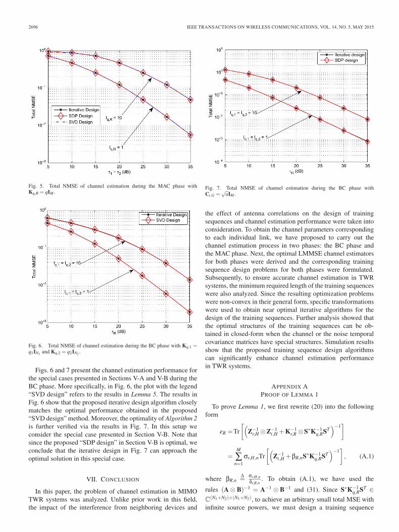
Fig. 5. Total NMSE of channel estimation during the MAC phase withKq,R = qIM .

Fig. 6. Total NMSE of channel estimation during the BC phase with Kq,1 =q1IN1 and Kq,2 = q2IN2 .

Figs. 6 and 7 present the channel estimation performance forthe special cases presented in Sections V-A and V-B during theBC phase. More specifically, in Fig. 6, the plot with the legend“SVD design” refers to the results in Lemma 5. The results inFig. 6 show that the proposed iterative design algorithm closelymatches the optimal performance obtained in the proposed“SVD design” method. Moreover, the optimality of Algorithm 2is further verified via the results in Fig. 7. In this setup weconsider the special case presented in Section V-B. Note thatsince the proposed “SDP design” in Section V-B is optimal, weconclude that the iterative design in Fig. 7 can approach theoptimal solution in this special case.

VII. CONCLUSION

In this paper, the problem of channel estimation in MIMOTWR systems was analyzed. Unlike prior work in this field,the impact of the interference from neighboring devices and

Fig. 7. Total NMSE of channel estimation during the BC phase withCt,G =

√aIM .

the effect of antenna correlations on the design of trainingsequences and channel estimation performance were taken intoconsideration. To obtain the channel parameters correspondingto each individual link, we have proposed to carry out thechannel estimation process in two phases: the BC phase andthe MAC phase. Next, the optimal LMMSE channel estimatorsfor both phases were derived and the corresponding trainingsequence design problems for both phases were formulated.Subsequently, to ensure accurate channel estimation in TWRsystems, the minimum required length of the training sequenceswere also analyzed. Since the resulting optimization problemswere non-convex in their general form, specific transformationswere used to obtain near optimal iterative algorithms for thedesign of the training sequences. Further analysis showed thatthe optimal structures of the training sequences can be ob-tained in closed-form when the channel or the noise temporalcovariance matrices have special structures. Simulation resultsshow that the proposed training sequence design algorithmscan significantly enhance channel estimation performancein TWR systems.

APPENDIX APROOF OF LEMMA 1

To prove Lemma 1, we first rewrite (20) into the followingform

eR =Tr

[(Z−1

r,H ⊗Z−1t,H +K−1

r,R ⊗S∗K−1q,RST

)−1]

=M

∑n=1

σr,H,nTr

[(Z−1

t,H +βR,nS∗K−1q,RST

)−1], (A.1)

where βR,nΔ=

σr,H,nδr,R,n

. To obtain (A.1), we have used the

rules (A ⊗ B)−1 = A−1 ⊗ B−1 and (31). Since S∗K−1q,RST ∈

C(N1+N2)×(N1+N2), to achieve an arbitrary small total MSE with

infinite source powers, we must design a training sequence


S achieving a full rank S∗K−1q,RST , which implies that the

minimum length of Si must satisfy Ls ≥ N1 +N2. Otherwise,based on the fact Rank(AB) ≤ min{Rank(A),Rank(B)}, wemust have Rank(S∗K−1

q,RST ) ≤ LS < N1 +N2. Let us consider

the case where S∗K−1q,RST has a maximum rank of Ls (which will

lead to the MSE lower bound as shown below). In this case, theMSE in (A.1) can be lower bounded by

eR ≥M

∑n=1

σr,H,n

×(

Ls

∑m=1

1

σ−1t,H,m +βR,nλSK,m

+N1+N2

∑m=LS+1

σt,H,m

), (A.2)

where λSK,m is the m-th element of λ(S∗K−1q,RST ). Moreover, the

eigenvlaues in {σt,H,m} and {λSK,m} are assumed to be arrangedin a decreasing order, respectively. To obtain (A.2), we have usethe fact that the function Tr(A−1) is a schur convex functionwith respect to the eigenvalues of A and the following resultfrom [27] λ(−1

r,H)+λ(S∗K−1q,RST ) � λ(Z−1

r,H +S∗K−1q,RST ). When

the source power tends to infinity, the term ∑Lsm=1

1σ−1

t,H,m+βR,mλSK,m

in (A.2) approaches zero. Thus, eR in (A.2) is lower bounded by∑M

n=1 σr,H,n ∑N1+N2m=LS+1 σt,H,m.

If Kq,R = qI, the total MSE in (A.1) can be written as

eR =M

∑n=1

σr,H,nTr

[(Z−1

t,H + βR,nS∗ST)−1

], (A.3)

where βR,nΔ= βR,n/q. With a finite power at the source, it is

assumed that the optimal solution of S1 and S2 in (25) resultsin the optimal S, denoted by S, to have a rank of r ≤ N1 +N2.By using the SVD decomposition, the optimal S can be decom-posed to S = USΣSVH

S , where US and VS are matrices of size(N1+N2)×r and LS×r, respectively, with UH

S US = Ir, VHS VS =

Ir; ΣS is an r×r diagonal singular-value matrix. The optimal S1

and S2 can be denoted as S1 = US,1ΣSVHS and S2 = US,2ΣSVH

S ,

where US,1Δ= US(1 : N1, :) and US,2

Δ= US(N1 + 1 : N1 +N2, :).

Subsequently, a new S given by S = USΣS, can be obtainedthat achieves an equal total MSE as that of S, however, witha shorter training sequence length of LS = r. Furthermore, thenew S1 = US,1ΣS and S2 = US,2ΣS require the same power atthe sources nodes compared to S1 and S2. This completes theproof of Lemma 1.

APPENDIX BPROOF OF LEMMA 2

By taking the gradient of g(λi), we can easily verify thatg(λi) decreases with λi}. Next, we mainly focus on derivingthe upper bound of λi. The source power constraint can be re-written as

Tr(sisi)H =Tr

[(Xs,1 ⊗Xs,2,i +λiI)−2xs,3,ixH

s,3,i

]≤ σs,3,i

(σs,min,i +λi)2 , (B.1)

where σs,min,i and σs,3,i are defined in Lemma 2. In (B.1),the inequality is obtained based on the identity Tr(AB) ≤∑i σA,iσB,i [29]. Here, σA,i and σB,i are the eigenvalues ofthe n× n matrices A and B, respectively, {σA,1,σA,2, · · · ,σA,n}and {σB,1,σB,2, · · · ,σB,n} are arranged in the same order, andthe equality is achieved when A and B are diagonal matri-ces. Hence we have

σs,3,i

(σs,min,i+λi)2 ≥ τi, which further implies

λi ≤√

σs,3,iτi

−σs,min,i.

APPENDIX CPROOF OF THEOREM 2

In (46), the feasible set established by the power constraintsis convex since the function Tr(EiQS) is linear [25]. To provethe convexity of (46), it is sufficient to show that the objectivefunction is convex. Without loss of generality, we denote thatf (QS) = Tr[(Z−1

t,H +αnQS)−1]. Using the fact that a function is

convex if and only if it is convex when restricted to any line thatintersects its domain [25], we can prove the convexity of f (QS)by restricting it to an arbitrary line that intersects the domainS

N+, i.e., prove the convexity of g(t) = Tr[(Z−1

t,H + αn((1 −t)QS,1 + tQ′

S,2))−1] with respect to t where t ≥ 0, QS,1 and Q′

S,2

are two arbitrary given elements in SN+. Considering that g(t) =

Tr[(Z−1t,H +αn(QS,1+t(Q′

S,2−QS,1)))−1] with Q′

S,2−QS,1 ∈ SN ,

it is equivalent to prove g(t) = Tr[(Z−1t,H +αn(QS,1+tQS,2)))

−1]

with QS,2 ∈ SN is convex with respect to t. To this end, we first

have dg(t)dt = −Tr(αn(Z−1

t,H +αn(QS,1 + tQS,2))−2QS,2). Based

on that, we can further reach

d2g(t)dt2 =2α2

nTr

((Z−1

t,H +αn(QS,1 + tQS,2))−2

QS,2

×(

Z−1t,H +αn(QS,1 + tQS,2)

)−1QS,2

)≥ 0. (C.1)

To obtain (C.1), we use the fact that (Z−1t,H + αn(QS,1 +

tQS,2))−2 and QS,2(Z−1

t,H +αn(QS,1+tQS,2))−1QS,2 are positive

semidefinite matrices. Hence, we conclude that the functionf (QS) is convex with respect to the positive semidefinite matrixQS, which further implies that the objective function in (46) isconvex since the sum of multiple convex functions is a still aconvex function.

APPENDIX DPROOF OF THEOREM 3

For notation convenience, we define D0Δ=

Z−1t,H1

+ αnS∗ST and let D0 = Z−1t,H + αnS∗ST =[

Z−1t,H1

+αnS∗1ST

1 αnS∗1ST

2

αnS∗2ST

1 Z−1t,H2

+αnS∗2ST

2

]Δ=

[D1 DH

2D2 D3

].

According to the matrix inverse identity, we have

D−10 =

[A0 B0

C0 D0

], where A0 = (D1 − DH

2 D−13 D2)

−1,

B0 = −D−11 DH

2 (D3 − D2D−11 DH

2 )−1, C0 = −D−1

3 D2(D1 −DH

2 D−13 D2)

−1, and D0 = (D3 − D2D−11 DH

2 )−1. Subsequently,


we obtain that Tr(D−10 ) = Tr[(D1 −DH

2 D−13 D2)

−1] +Tr[(D3 −D2D−1

1 DH2 )

−1]. Since DH2 D−1

3 D2 � 0 and D2D−11 DH

2 � 0, theinequalities D1 −DH

2 D−13 D2 D1 and D3 −D2D−1

1 DH2 D3

hold, which further implies that

(D1 −DH

2 D−13 D2

)−1 �D−11 ,

(D3 −D2D−1

1 DH2

)−1 �D−13 , (D.1)

where in obtaining the above, we have used the fact that thematrices D1, D3, D1 − DH

2 D−13 D2 and D3 − D2D−1

1 DH2 are

positive semidefinite. From (D.1), we have

Tr[(

D1 −DH2 D−1

3 D2)−1

]�Tr

(D−1

1

),

Tr[(

D3 −D2D−11 DH

2

)−1]�Tr

(D−1

3

). (D.2)

Hence, if D2 = 0, i.e., S∗2ST

1 = 0, the value of the objectivefunction in (45) can be always reduced.

Next, we show that for any S1 and S2, letting S∗2ST

1 = 0does not increase the need for power at the source nodes.Since in (45), the value of the objective function and the powerconstraints are only affected by S∗

1ST1 and S∗

2ST2 , the optimal S1

and S2, denoted by S1 and S2, can be determined as

Si = Ut,siΣsiVHsi, i = 1,2 (D.3)

where Vsi can be any matrix satisfying VHsi

Vsi = I. It is worthnoting that as LS ≥ N1 +N2, one can always find a specific Vs1

and Vs2 such that

VHs1

Vs2 = 0, (D.4)

which further results in S∗2ST

1 = 0. In this case, we do not changethe value of S∗

i STi and the power constraint, while decrease

the value of the objective function according to (D.2). Thisindicates that the condition S∗

1ST2 = 0 is sufficient and necessary

for obtaining the optimal solution of (45).It is noticed that the orthogonal training sequences have also

been proven to be optimal for the cascaded channel estimationin two-way relaying system in [15] and [16]. Here, we showthat similar results hold for individual channel estimation. Withthe optimal condition S∗

1ST2 = 0, the optimization problem in

(45) can be decomposed into two subproblems given by

minSi

M

∑n=1

σr,H,nTr

[(Z−1

t,Hi+αnS∗

i STi

)−1]

s.t. Tr(S∗i ST

i )≤ τi, i = 1,2 (D.5)

Based on the results derived for point-to-point MIMO systems[18], we obtain that the unitary matrix Ut,si given in (D.3)should be of the form Ut,si = U∗

t,Hi, and Vs1 should satisfy

(D.4). Then, solving (D.5) just reduces to solving the a powerallocation problem with the optimal σsi,m being obtained via thewater-filling problem in (49).

REFERENCES

[1] R. Wang, H. Mehrpouyan, M. Tao, and Y. Hua, “Optimal training designand individual channel estimation for MIMO two-way relay systems incolored environment,” in Proc. IEEE Globecom. Austin, Texas, USA,2014.

[2] Y. Hua, D. W. Bliss, S. Gazor, Y. Rong, and Y. Sung, “Theories and meth-ods for advanced wireless relays: Issue I,” IEEE J. Sel. Areas Commun.,vol. 30, no. 8, pp. 1297–1303, Sep. 2012.

[3] T. Kong and Y. Hua, “Optimal design of source and relay pilots for MIMOrelay channel estimation,” IEEE Trans. Signal Process., vol. 59, no. 9,pp. 4438–4446, Sep. 2011.

[4] F. Gao, R. Zhang, and Y.-C. Liang, “Optimal channel estimation and train-ing design for two-way relay networks,” IEEE Trans. Commun., vol. 57,no. 10, pp. 3024–3033, Oct. 2009.

[5] S. Abdallah and I. Psaromiligkos, “Partially-blind estimation of reciprocalchannels for AF two-way relay networks employing M-PSK modulation,”IEEE Trans. Wireless Commun., vol. 11, no. 5, pp. 1649–1654, May2012.

[6] S. Abdallah and I. Psaromiligkos, “Blind channel estimation for amplify-and-forward two-way relay networks employing M-PSK modulation,”IEEE Trans. Signal Process., vol. 60, no. 7, pp. 3604–3615, Mar. 2012.

[7] G. Wang, F. Gao, W. Chen, and C. Tellambura, “Channel estimationand training design for two-way relay networks in time-selective fadingenvironments,” IEEE Trans. Wireless Commun., vol. 10, no. 8, pp. 2681–2691, Aug. 2011.

[8] F. Gao, R. Zhang, and Y.-C. Liang, “Channel estimation for OFDM mod-ulated two-way relay networks,” IEEE Trans. Signal Process., vol. 57,no. 11, pp. 4443–4455, Nov. 2009.

[9] S. Zhang, F. Gao, and C.-X. Pei, “Optimal training design for individ-ual channel estimation in two-way relay networks,” IEEE Trans. SignalProcess., vol. 60, no. 9, pp. 4987–4991, Sep. 2012.

[10] R. Wang and M. Tao, “Joint source and relay precoding designs for MIMOtwo-way relaying based on MSE criterion,” IEEE Trans. Signal Process.,vol. 60, no. 3, pp. 1352–1365, 2012.

[11] S. Xu and Y. Hua, “Optimal design of spatial source-and-relay matricesfor a non-regenerative two-way MIMO relay system,” IEEE Trans. Wire-less Commun., vol. 10, no. 5, pp. 1645–1655, May 2011.

[12] J. Zhao, M. Kuhn, A. Wittneben, and G. Bauch, “Self-interferenceaided channel estimation in two-way relaying systems,” in Proc. IEEEGLOBECOM, New Orleans, LO, USA, Dec. 2008, pp. 1–6.

[13] Z. Fang, J. Shi, and H. Shan, “Comparison of channel estimation schemesfor MIMO two-way relaying systems,” in Proc. CSQRWC, Harbin, China,Jul. 2011, pp. 719–722.

[14] T.-H. Pham, Y.-C. Liang, A. Nallanathan, and H. K. Garg, “Optimaltraining sequences for channel estimation in bi-directional relay networkswith multiple antennas,” IEEE Trans. Commun., vol. 58, no. 2, pp. 474–479, Feb. 2010.

[15] D.-H. Kim, M. Ju, and H.-M. Kim, “Optimal training signal designfor estimation of correlated MIMO channels in two-way amplify-and-forward relay systems,” IEEE Commun. Lett., vol. 17, no. 3, pp. 491–494,Mar. 2013.

[16] C. Chiong, Y. Rong, and Y. Xiang, “Channel training algorithms for two-way MIMO relay systems,” IEEE Trans. Signal Process., vol. 61, no. 16,pp. 3988–3998, Aug. 2013.

[17] M. Biguesh, S. Gazor, and M. Shariat, “Optimal training sequence forMIMO wireless systems in colored environments,” IEEE Trans. SignalProcess., vol. 57, no. 8, pp. 3144–3153, Aug. 2009.

[18] E. Bjornson and B. Ottersten, “A framework for training-based estimationin arbitrarily correlated rician MIMO channels with rician disturbance,”IEEE Trans. Signal Process., vol. 58, no. 3, pp. 1807–1820, Mar. 2010.

[19] R. Wang, M. Tao, and Z. Xiang, “Nonlinear precoding design for MIMOamplify-and-forward two-way relay systems,” IEEE Trans. Veh. Technol.,vol. 61, no. 9, pp. 3984–3995, Nov. 2012.

[20] R. Wang, M. Tao, and Y. Huang, “Linear precoding designs for amplify-and-forward multiuser two-way relay systems,” IEEE Trans. WirelessCommun., vol. 11, no. 12, pp. 4457–4469, Dec. 2012.

[21] Y. Liu, T. Wong, and W. W. Hager, “Training signal design for estimationof correlated MIMO channels with colored interference,” IEEE Trans.Signal Process., vol. 55, no. 4, pp. 1486–1497, Apr. 2007.

[22] D. Chizhik et al., “Multiple-input-multiple-output measurements andmodeling in manhattan,” IEEE J. Sel. Areas Commun., vol. 21, no. 3,pp. 321–331, Apr. 2003.

[23] K. Yu et al., “A wideband statistical model for nlos indoor MIMOchannels,” in Proc. IEEE VTC Spring, Birmingham, U.K., May 2002,pp. 370–374.

[24] S. M. Kay, Fundamentals of Statistical Signal Processing: EstimationTheory. Englewood Cliffs, NJ, USA: Prentice-Hall, 1993.


[25] S. Boyd and L. Vandenberghe, Convex Optimization. Cambridge, U.K.:Cambridge Univ. Press, 2004.

[26] J. Yeh, Real Analysis: Theory of Measure and Integration, 2nd ed.Singapore: World Scientific, 2006.

[27] E. Jorswieck and H. Boche, Majorization and Matrix-Monotone Func-tions in Wireless Communications. Delft, The Netherlands: NowPublishers Inc., 2007.

[28] K. B. Petersen and M. S. Pedersen, “The matrix cookbook.” Techni-cal University of Denmark, Nov. 2012, Version 20121115. [Online].Available: http://www2.imm.dtu.dk/pubdb/p.php?3274.

[29] J.-B. Lasserre, “A trace inequality for matrix product,” IEEE Trans.Autom. Control, vol. 40, no. 8, pp. 1500–1501, Aug. 1995.

Rui Wang (M’14) received the B.S. degree fromAnhui Normal University, Wuhu, China, in 2006,and the M.S. degree from Shanghai University,Shanghai, China, in 2009 and the Ph.D. degree fromShanghai Jiao Tong University, China, in 2013, allin electronic engineering. From August 2012 toFebruary 2013, he was a visiting Ph.D. student withthe Department of Electrical Engineering, Universityof California, Riverside, CA, USA. From October2013 to October 2014, he was with the Instituteof Network Coding, The Chinese University of

Hong Kong as a Postdoctoral Research Associate. Since October 2014, he hasbeen an Assistant Professor with the College of Electronics and InformationEngineering, Tongji University. His research interests include wireless cooper-ative communications, MIMO technique, network coding, and OFDM etc.

Meixia Tao (S’00–M’04–SM’10) received the B.S.degree in electronic engineering from Fudan Univer-sity, Shanghai, China, in 1999, and the Ph.D. degreein electrical and electronic engineering from HongKong University of Science and Technology in 2003.She is currently a Professor with the Department ofElectronic Engineering, Shanghai Jiao Tong Univer-sity, China. Prior to that, she was a Member of Pro-fessional Staff at Hong Kong Applied Science andTechnology Research Institute during 2003–2004,and a Teaching Fellow then an Assistant Professor at

the Department of Electrical and Computer Engineering, National University ofSingapore from 2004 to 2007. Her current research interests include cooperativecommunications, wireless resource allocation, MIMO techniques, and physicallayer security.

Dr. Tao is an Editor for the IEEE TRANSACTIONS ON COMMUNICATIONS

and the IEEE WIRELESS COMMUNICATIONS LETTERS. She was on the Edi-torial Board of the IEEE TRANSACTIONS ON WIRELESS COMMUNICATIONS

from 2007 to 2011 and the IEEE COMMUNICATIONS LETTERS from 2009 to2012. She also served as Guest Editor for IEEE COMMUNICATIONS MAGA-ZINE with feature topic on LTE-Advanced and 4G Wireless Communicationsin 2012, and Guest Editor for EURISAP J WCN with special issue on PhysicalLayer Network Coding for Wireless Cooperative Networks in 2010.

Dr. Tao is the recipient of the IEEE Heinrich Hertz Award for Best Commu-nications Letters in 2013, the IEEE ComSoc Asia-Pacific Outstanding YoungResearcher Award in 2009, and the International Conference on WirelessCommunications and Signal Processing (WCSP) Best Paper Award in 2012.

Hani Mehrpouyan (S’05–M’10) received the B.Sc.honours degree from Simon Fraser University,Burnaby, Canada, in 2004 and the Ph.D. degree fromQueens University, Kingston, Canada, in electricalengineering in 2010. From September 2010 to March2012 he was a Post-Doc at Chalmers University ofTechnology, where he led the MIMO aspects of themicrowave backhauling for next generation wirelessnetworks project. He next joined the University ofLuxembourg as a Research Associate from April2012 to August 2012, where he was responsible

for new interference cancellation and synchronization schemes for satellitecommunication links. Since 2012, he has been an Assistant Professor at Cal-ifornia State University, Bakersfield, CA, USA. His current research interestslie in the area of applied signal processing and physical layer of wirelesscommunication systems, including millimeter-wave systems, reconfigurableantennas, energy harvesting systems, synchronization, and channel estimation.For more information refer to www.mehrpouyan.info.

Dr. Mehrpouyan has more than 40 publications in prestigious IEEE jour-nals and conferences. He is an Associate Editor of IEEE COMMUNICATION

LETTERS and he has also served as a TPC member for IEEE Globecom, ICC,VTC, etc. He has also been involved with industry leaders such as EricssonAB, Blackberry etc. He has received many scholarships and awards, e.g., IEEEGlobecom Early Bird Student Award, NSERC-IRDF, NSERC PGS-D, NSERCCGS-M Alexander Graham Bell, B.C. Wireless Innovation, and more.

Yingbo Hua (S’86–M’88–SM’92–F’02) receivedthe B.S. degree from Southeast University, Nanjing,China, in 1982 and the Ph.D. degree from SyracuseUniversity, Syracuse, NY, USA, in 1988. He held afaculty position with the University of Melbourne,Australia, where he was promoted to the rank ofReader and Associate Professor from 1996. He wasa Visiting Professor with Hong Kong University ofScience and Technology (1999–2000), and a Con-sultant with Microsoft Research, WA, USA (summer2000). Since 2001, he has been a Professor with the

University of California at Riverside.Dr. Hua has served as Editor, Guest Editor, Member of Editorial Board

and/or Member of Steering Committee for IEEE TRANSACTIONS ON SIG-NAL PROCESSING, IEEE SIGNAL PROCESSING LETTERS, EURASIP SignalProcessing, IEEE SIGNAL PROCESSING MAGAZINE, IEEE JOURNAL OF

SELECTED AREAS IN COMMUNICATIONS, and IEEE WIRELESS COMMU-NICATION LETTERS. He has been a Member of IEEE Signal ProcessingSociety’s Technical Committees for Underwater Acoustic Signal Processing,Sensor Array and Multichannel Signal Processing, and Signal Processing forCommunication and Networking. He has served on Technical and/or Organiz-ing Committees for over 50 international conferences and workshops. He hasauthored/coauthored over 300 articles and coedited three volumes of books,with more than 8000 citations, in the fields of Sensing, Signal Processing andCommunications. He is a Fellow of AAAS.

channel estimation and optimal training design for

Documents