a model for multi-year combined optimal …shamir.net.technion.ac.il/files/2012/04/miki-zaide...a...
TRANSCRIPT

A Model for Multi-Year Combined Optimal Management of Quantity
and Quality in the Israeli National Water Supply
System
Michael Zaide

A Model for Multi-Year Combined Optimal Management of Quantity
and Quality in the Israeli National Water Supply
System
Research Thesis
Submitted in Partial Fulfillment of the
Requirements for the
Degree of Master of Science in
Engineering and Management of Water Resources
by
Michael Zaide
Submitted to the Senate of the Technion - Israel Institute of Technology
Shvat 5766 Haifa February 2006

Acknowledgements
The Research Thesis was done under the Supervision of Prof. Uri Shamir in the
Department of Environmental and Water Resources, Faculty of Civil and
Environmental Engineering, Technion – Israel Institute of Technology.
I was privileged to be supervised by Prof. Uri Shamir and I would like to express my
deep thanks and appreciation for the inspiration and the thrilling moments
experienced during his guidance which extended far beyond the research subject to
many other issues of water management.
I would also like to thank Dr. Joseph Dreizin (former manager of the Planning
Division, Water Commission) who strongly encouraged me to study water
management and enabled me to combine work and studies.
I’m grateful to Mo Provisor (current manager of the Planning Division, Water
Commission) for his encouragement and support.
I wish to thank the Water Commission which participated in financing my studies.
I wish to thank my family for their patience and support, especially my mother who
helped with the proof-reading of this thesis.

Table of contents (continuance) page
3.5.1 Policy Principals------------------------------------- ----------------------------------------50
3.5.1.1 Demand Policy---------------------------------- -----------------------------------------50
3.5.1.2 Development Policy---------------------------- -----------------------------------------52
3.5.1.3 Sources Management Policy------------------------------------------------------------53
3.5.2 Aggregation and Simplification------------------------------------------------------------54
3.5.3 Optimization vs. Simulation----------------------------------------------------------------54
3.5.4 Incorporating Sustainability Considerations---- -----------------------------------------56
3.5.4.1 Prescribed System States at Selected Times------------------------------------------56
3.5.4.2 Time Horizon and Time Representation----------------------------------------------56
3.5.4.3 Incorporating Uncertainty Considerations--------------------------------------------57
3.5.4.4 Reliability---------------------------------------------------------------------------------57
3.5.4.5 Calibration-------------------------------------------------------------------------------- 58
3.6 Model’s Structure and Input--------------------------------------------------------------------58
3.6.1. Supply Data----------------------------------------------------------------------------------59
3.6.1.1 Replenishment----------------------------------------------------------------------------59
3.6.1.2 Water Sources Data----------------------------------------------------------------------59
3.6.2 Demand Data---------------------------------------------------------------------------------60
3.6.3 Conveyance System Data-------------------------------------------------------------------60
3.6.4 Sources Management Data------------------------------------------------------------------61
3.6.5 Development Policy Management Data------------------------------------------------- 61
3.6.6 Initial Values----------------------------------------------------------------------------------61
3.7 Model Output-------------------------------------------------------------------------------------62
3.8 Optimization Method and the Software Used------------------------------------------------63
Chapter 4: Mathematical Formulation of the Model----------------------------------------65
4.1 Introduction---------------------------------------------------------------------------------------65
4.2 Model Dimensions-------------------------------------------------------------------------------65
4.3 Decision Variables-------------------------------------------------------------------------------66
4.4 Constraints------------------------------------------------ ----------------------------------------69
4.4.1 Hydrological Constraints--------------------------------------------------------------------69
4.4.1.1 Water Level Constraints-----------------------------------------------------------------73
4.4.1.2 Aquifer Salinity Constraints------------------------------------------------------------74

Table of contents (continuance 2) page
4.4.1.3 Spills in Lake Kinneret------------------------------------------------------------------74
4.4.2 Demand --------------------------------------------------------------------------------------74
4.4.2.1 Minimum Demand in Consumer Zones -------------------------------------------74
4.4.2.2 Prescribed Quality of the water supplied to Consumer Zones-----------------75
4.4.3 Conveyance System------------------------------------------------------------------------75
4.4.3.1 Conveyance Capacity ------------------------------------------------------------75
4.4.3.2 Quantity Conservation -----------------------------------------------------------76
4.4.3.3 Mass Conservation ----------------------------------------------------------------76
4.4.3.4 Desalination Capacity-------------------------------------------------------------77
4.4.3.5 Desalinated Water Quality--------------------------------------------------------77
4.4.4 State Variables-----------------------------------------------------------------------------78
4.4.5 Non Negative Variables------------------------------------------------------------------ 79
4.5 Objective Function-------------------------------------------------------------------------------79
4.5.1 Definition of Conveyance Cost ---------------------------------------------------------81
4.5.2 Extraction Levy----------------------------------------------------------------------------81
4.5.3 Desalination Cost--------------------------------------------------------------------------83
Chapter 5: Examples of the Models’ Results------------------------------------------------- 84
5.1 Introduction -------------------------------------------------------------------------------------- 84
5.2 Results of the Annual Model------------------------------------------------------------------- 84
5.2.1 Base Run------------------------------------------------------------------------------------84
5.2.2 Scenarios Description---------------------------------------------------------------------87
5.2.3 Analysis of the Results--------------------------------------------------------------------87
5.3 Multi –Year Run -------------------------------------------------------------------------------104
5.3.1 Review of the Results -------------------------------------------------------------------104
5.4 Conclusions Drawn from the Annual and Multi-Year Runs -----------------------------108
Chapter 6: Conclusions and Discussion-------------------------------------------------------110
6.1 Modeling and General Conclusions ---------------------------------------------------------110
6.2 Strategic Conclusions--------------------------------------------------------------------------111
6.3 National Planning Implications---------------------------------------------------------------112

Table of contents (continuance 3) page
Chapter 7: Recommendation for Future Development ----------------------------------113
References 115
List of Tables
Table 1.1 - The Water Balance of the Israeli Water Sector (until 2020) --------------------- 14
Table 1.2 - Development Program by 2010-------------------------------------------------------15
Table 2.1 - Summary Table of National (or large regional) Level Models-------------------39
Table 5.1- Initial Conditions for the Annual Base Run----------------------------------------- 86
Table 5.2 - Annual model - Scenarios List------------------------------------------------------- 87
Table 5.3 - Annual model -Main Results ---------------------------------------------------------91
Table 5.4 - Multi–Year Run - Development Program -----------------------------------------104
Table 5.5: Multi–Year Model - Components of the Objective Function -------------------106
List of Figures
Figure 1.1 - Rainfall Variability in Israel ---------------------------------------------------------- 9
Figure 1.2 - The Main Natural Water Sources and their Average Annual Yield ----------- 10
Figure 1.3 - Replenishment Time Series 1932-2002-------------------------------------------- 10
Figure 1.4 - Total Demand by Sectors in 2003---------------------------------------------------11
Figure 1.5 - National Water Supply System -----------------------------------------------------12
Figure 1.6 - Salinity and Nitrates in the Coastal Aquifer-------------------------------------- 13
Figure 1.7 - The Development and Deployment of Sea Water Desalination Plants---------15
Figure 2.1- MMA – Inter Regional Water Flows In Israel--------------------------------------24
Figure 2.2 - Schematic Representation of the ‘Aggregative Model’ ------------------------- 25
Figure 2.3 - The Topology of the TBS Model----------------------------------------------------29
Figure 2.4 - CALVIN – Inter Regional Water Flows In California--------------------------- 32
Figure 2.5 - Data flow in the Calvin Model----------------------------------------------------- 32
Figure 3.1 - Model Topology----------------------------------------------------------------------- 52
Figure 3.2 - Input – Output Data--------------------------------------------------------------------64
Figure 4.1 - Time Scheme for the Multi –Annual Model-------------------------------------- 65

Figure 4.2 - Flow Direction Coefficient-----------------------------------------------------------73
Figure 4.3 - Sensitivity of k Coefficient-----------------------------------------------------------73
Figure 4.4 - Definition sketch for the Extraction Levy -----------------------------------------82
Figure 5.1 - Scenario 1 - Base Run (B.R.) - flow chart season 1-------------------------------92
Figure 5.2 - Scenario 1 - Base Run (B.R.) - flow chart season 2-------------------------------93
Figure 5.3 - Scenario 2 - B.R. + 1m in MA - flow chart season 1 -----------------------------94
Figure 5.4 - Scenario 2 - B.R. + 1m in MA - flow chart season 2 ---------------------------- 95
Figure 5.5 - Scenario 3 - B.R+150 MCM/Y in LKB - flow chart season 1 ------------------96
Figure 5.6 - Scenario 3 - B.R+150 MCM/Y in LKB - flow chart season 2 ------------------97
Figure 5.7 - Scenario 4 - B.R+100MCM/Y Negev - flow chart season 1 --------------------98
Figure 5.8 - Scenario 4 - B.R+100MCM/Y Negev - flow chart season 2---- ----------------99
Figure 5.9 - Scenario 5 - B.R. +150 mg Cl- li Gush Dan+ 45des pal
flow chart season 1 -------------------------------------------------------------------100
Figure 5.10 - Scenario 5: B.R. +150 mg Cl- li Gush Dan+ 45des pal –
flow chart season 2----------------------------------------------------------------- 101
Figure 5.11 - Scenario 6: B.R. +150 mg Cl- li Gush Dan+ 45des Pal
+ KY 250 mg Cl- li Flow chart season 1---------------------------------------- 102
Figure 5.12 - Scenario 6: B.R. +150 mg Cl- li Gush Dan+ 45des Pal
+ KY 250 mg Cl- li Flow chart season 2-----------------------------------------103
Figure 5.13 - Multi-Year Model - Sources Water Level---------------------------------------106
Figure 5.14 - Multi-Year Model – Lake Kinneret Water Level-------------------------------107
Figure 5.15 - Multi-Year Model – Salinity in the Water Sources---------------------------- 107
Figure 5.16 - Multi-Year Model – Desalination Usage--------------------------------------- 108
Figure 5.17- Multi-Year Model - Desalination Efficiency------------------------------------ 108

1
Abstract
Israel has entered the desalination era once it became obvious that the natural resources
do not suffice to meet the needs of today, and of a sustainable future. The depletion of
the natural resources has been exacerbated by deterioration of the groundwater in the
main aquifers. With desalination becoming an important addition to the supply system,
and water quality gaining increasing importance, it is necessary to develop tools for
management of the national water system which consider both quantity and quality of
water in the sources and in the supply systems.
Most models for water management operated in the Water Sector were focused on the
quantitive aspects of the national water sector almost without addressing the salinity
considerations along the system: especially the salinity concentration in the water
sources and in the demand zones.
In this work a seasonal multi-year model for management (planning and operation) of
both water quantity and quality in the Israeli National Supply System (INWSS) has
been developed. For the first time, both quantity and quality (salinity) considerations
(water sources, supply system and demand zones) are optimized simultaneously for a
long term time horizon (10-20 years and more). The model is called: Multi-Year
Combined Optimal Management of Quantity and Quality in the
Israeli National Water Supply System (MYCOIN).
The model seeks the seasonal operating plan for this time horizon which minimizes a
cost function that combines actual operational costs, including the extraction levy
placed on production of water from the natural sources, with penalties for not using the
full capacity of desalination plants (as per the contracts with the private companies that
construct and operate them), a penalty for deficits in supplying the demands, and a
penalty for water spilled from the Kinneret.
The operating plan is subject to constraints of various types, including: capacities of
the sources and the conveyance system, capacity and removal ratio of the desalination
plants, demands to be met and their required salinities, the physical laws of water and
salt mass conservation in the aquifers and in the supply system, and limits of levels and
salinities in the sources. Sequential seasons are linked through the values of state
variables: water levels and salinities in the sources.

2
While the model deals with the operational plan with a given physical supply system,
the optimization yields insights with respect to the planning of the system itself, such
as:
� Adequacy of the installed capacity of desalination plants.
� Adequacy of the removal ratio (outlet salinity) of the desalination plants.
� The required 'salinity map' in the supply system which is required to meet salinity
constraints at consumer nodes and maintain aquifer salinity limits.
� Installed capacities of production and conveyance facilities.
The solution reports can indicate some of the planning needs ("bottle-necks") by
analysis of the results and examination of shadow prices.
The objective function and some of the constraints in the model that has been
developed is non-linear. Discontinuous functions have been "smoothed" by a
transformation that maintain acceptable accuracy of the smoothed function yet results
in a differentiable function that can be handled by the optimization software. The
model is solved by LSGRG (Large Scale Generalized Gradient), an off-the-shelf
software that uses EXCEL for model formulation.
Two versions of the model have been implemented: an annual model with two seasons,
and a multi-year model that covers the coming three years one-by-one, and then two
more "Future Reference Years" (FRYs). Each FRY represents a number of years
(typically 3-7, but they can be longer), which repeat themselves and bring into the
operational model the considerations of a longer time horizon. The multi-year model
therefore has 5 annual periods: the first 3 years to come plus two FRYs.
The annual model has 420 decision variables and 156 constraints. The multi-year
Model, which covers five years, has 2100 decision variables and 780 constraints (not
including upper and lower bounds – 4200 altogether). Its output is presented in
schematics of the system, on which are placed flows (seasonal quantities) and their
associated salinities, as well as source water levels and salinities, as well as in
"management reports" which facilitate comprehension of the results.
The model is considered to be one component in a "Model Hierarchy" (Shamir, 1971,
1972) that is being developed for and utilized by the Water Commission, which range

3
from highly aggregated models of the entire national water system to much more
detailed (in space and time) models of regional systems.
The model was developed with available data, not all of which is considered accurate
and final. Model results should be viewed accordingly.
The main conclusions from the models’ runs are:
1. It is possible to solve jointly by optimization quantity and quality issues.
2. It is possible to solve the quantity and quality problem by off the shelf software
(Frontline’s Solver).
3. The model is for optimizing the operation – with planning implications.
4. It is possible to:
a. Prove whether the stated quality and quantity targets can be achieved.
b. Indicate and test the means for achieving these targets.
5. The solution can change - sometimes quite dramatically - when salinity
considerations are imposed.
Concerning management of the INWSS the conclusions are:
1. This is the first time the national system is optimized over a period of many years
considering both quantity and quality (salinity).
2. In addition to the regular water management policy there is a need to adopt a water
quality management policy, expressed by salinity targets at the demand zones and
in the natural sources.
3. The development program should be determined with consideration of the water
quality management policy, and may be affected quite substantially by it.

4
List of Symbols
t
noC - The average salinity in node no at season t (mg Cl-/liter).
t
CCC - The average salinity in Center Coastal Aquifer (mg Cl-/liter).
t
nCin - The average salinity entered to the aquifer n (mg Cl-/liter).
t
nCout - The average quality of water that exits the aquifer n (mg Cl-/liter).
1−tn
t
nCC - The average water salinity in Aquifer n in season t and t-1 respectively
(mg Cl-/liter).
t
rC - The salinity of each source r=1...R (mg Cl-/liter).
t
dDef - Deficit of water to demand zone d in season t (MCM).
tnh - Water table in aquifer n in season t (m).
nhmix - Mixing volume coefficient in aquifer n.
thcc - Water table in CCA (m).
cchmix - The coefficient of the mixing volume in CCA.
tCChspill - Spill level above the bottom of the aquifer cell (m).
CCK - The spill coefficient from CCA to the sea (MCM/day).
→t
kdir - A direction coefficient that gets the value 0 or 1.
tKinspill - The extent of spills in Kinneret in season t (MCM).
t
lQ - Quantity that supplied in pipe l in season t (MCM).
t
noQartnode - Artificial source in node no in season t (MCM).
t
nodeQartmassno - Artificial mass in node no in season t (Ton Cl-).
t
ccQartmass - Artificial mass source (Ton Cl-).
t
nQartnode - Artificial source in source n in season t (MCM).
t
dQartmzone - Artificial mass in zone d in season t (Ton Cl-).
t
iQdes - The extent of desalination use in plant i in season t (MCM).
t
nQin - Recharge into natural aquifer n in season t (MCM).

5
t
nQout - Extraction from aquifer n in season t (MCM).
t
rQ - Replenishment and recharge of water from sources and pipes r=1....R (MCM).
tQp - The extraction from aquifer cell in season t (MCM).
t
iRR - The removal ratio of salt in desalination plant i in season t.
nSA - Aquifer’s n coefficient of storativity (MCM/m).
T∆ - The number of days per season (day).
T
Vn
∆
∆- The change in the aquifer’s n volume in the period T∆ (MCM/Season).
T
CVn
∆
∆- The change of mass in an aquifer n in the period T∆ (Ton Cl
-/Season).

6
List of Abbreviations
No. Abbreviation Full Text
1 ASL Above Sea Level
2 AV Artificial Variable
3 BR Base Run
4 BWDP Brackish Water Desalination Plant
5 CA Coastal Aquifer
6 CAN Coastal Aquifer North
7 CCA Central Coastal Aquifer
8 CAS Coastal Aquifer South
9 FRY Future Representative Year
10 GA Genetic Algorithm (GA)
11 GD Gush Dan
12 GRG Generalized Reduced Gradient
13 GUI Geographic User Interface
14 JK Jordanian Kingdom
16 KY Kfar Yehoshua
17 LB Lower Bound
18 LK Lake Kinneret
19 LP Linear Programming
20 LKB Lake Kinneret Basin
21 LSGRG Large Scale GRG
22 MA Mountain Aquifer
23 NC National Carrier
25 NCA North Coastal Aquifer
24 NPV Net Present Value
26 NWSS National Water Supply System
27 OF Objective Function
28 PA Palestinian Authority
29 PV Present Value
30 RR Removal Ratio
31 RSM Regional Simulation Model
32 SFWMD South Florida Water Management District
33 SWDP Sea Water Desalination Plant
34 TBM Tri Basin Model
35 TBS Three Basin System
36 UB Upper Bound
37 WG West Galilee

7
Chapter 1: Introduction
1.1 Preface
The water sector in Israel will face huge changes in the coming decades regarding its
structure and in many aspects of managing the Israeli National Water Supply System
(NWSS). The main challenges facing the Israeli water sector regarding quantity and
quality issues are:
a. Assuring reliability of supply.
b. Restoration and preservation of the natural sources.
c. Managing the water sector for long-term sustainability.
On the basis of the Water Sector Master Plan for the years 2002-2010 (Water
Commission, 2002),the government of Israel decided to build sea water desalination
plants SWDP with an installed capacity of 315 MCM/Year and to import 50-100
MCM/Year from Turkey. In addition, 50 MCM/Year of brackish water will be
desalinated and over 500 MCM /Year of wastewater will be reclaimed by 2010 mainly
for agricultural use (Table 1.1). A large part of the desalination program will be carried
out by the private sector; this will raise the challenge of efficient regulation and
management.
The Israeli NWSS is a relatively small yet complex system to manage and optimize.
The system comprises aquifers, a main surface reservoir – Lake Kinneret, desalination
plants, a central conveyance system and local distribution systems.
The consumers are urban, industry, agriculture, nature, and commitments under
Bilateral Agreements (with the Jordanian Kingdom (JK) and the Palestinian Authority
(PA)). The various consumers have different requirements regarding reliability, quality
of water supplied and the ability to pay for it.
The conveyance system is limited and the complexity of management, operation and
design of the Israeli NWSS will increase when quality considerations are taken into
account, especially when sustainable development policy considerations are
incorporated in cost–benefit analyses. A sustainable policy means meeting the needs of
the present without compromising the ability to meet the needs of future generations.

8
An example of a sustainable development issue relating to the preservation of the
natural resources is the "Salt Balance" issue. It is necessary to define the technical and
economic tools for reducing the amounts of salt accumulated in the natural sources,
especially in the Coastal Aquifer (CA). One proposal is to remove salts from the
reclaimed sewage; another option is to treat the water supplied for domestic use, so that
the wastewater has less salt content. Each alternative has its advantages and
disadvantages, technically and economically.
Tasks like these lead us to the need for long term (multi-year) multi-quality tools for
management of the Israeli NWSS under conditions of uncertainty and subject to a
policy of sustainable development. It does not seem feasible, nor desirable, to create
one tool that deals with all tasks simultaneously. The preferred option is to use a set of
models inter-connected in a well defined hierarchy.
The tool developed in this work can be part of this 'model hierarchy', which is already
in use at the Water Commission, and can contribute to strategic planning processes,
answering questions concerning operating and planning problems of policy while
taking into account the combined considerations of water quantity and quality.
1.2 The Israeli Water Sector and the National Water Supply System (NWSS)
Israel is located in a semi-arid to arid region (Gvirtzman 2002). The natural water
sources are replenished by an average of 500 mm of rain per year, ranging from over
1,000 mm/year to 150 mm/year over a distance of some 500 km (see Figure 1.1).

9
Figure 1.1 – Rainfall Variability in Israel
(Gvirtzman, 2002).
The average annual renewal potential of fresh water is 1555 MCM/Year (Water
Commission, 2005) . The main natural sources are Lake Kinneret (LK), the Mountain
Aquifer (MA) and the Coastal Aquifer (CA). Most of the supply depends on these
three sources, and the national system is therefore called the ‘Three Basin System’
(TBS). There are some additional natural sources which are connected to the TBS: the
Carmel and Western Galilee aquifers, and the Negev. The Arava basin is not connected
to the main water system.

10
Figure 1.2 – The Main Natural Water Sources and their Average Annual Yield
(MCM/YEAR) (Water Commission, 2005).
The difficulty of supplying a reliable quantity of water is due to the high variability of
annual replenishment, and the appearance of relatively long sequences of below
average years, as can be seen in Figure 1.3. The average over the period 1932-2002 is
around 1,457 MCM/Year, with a standard deviation of 458 MCM/Year. It has been as
low as 657 (1951) and as high as 3563 MCM/Year (1992).
Figure 1.3 – Replenishment Time Series 1932-2002
(Planning Division, Water Commission, 2002).
The Coastal Aquifer (CA) functions as the main over-year reservoir, while the other
sources have a lower over-year capacity.
Total annual potential
–) average(production
MCM1,555
Kinneret basins 650
Eastern basins
130
Negev Basin
Arava Basin
Western Galilee Aquifer - 110
Carmel Aquifer - 25
The Coastal Aquifer - 250
Mountain
Aquifer - 320
70

11
In 2003 the total demand of all sectors for all types of water was 1860 MCM (Figure
1.4, Water Commission, 2004) - 1,377 MCM/Year of potable water and 483
MCM/Year of sub-potable water (reclaimed wastewater and brackish waters). Urban
consumption already exceeds 50% of the total potable water use, and keeps rising at a
rate of approximately 20 MCM/Year. Potable water use by agriculture is close to the
goal set by the government of 530 MCM/Year; this residual agriculture is much less
flexible regarding to water shortage.
Potable
562.5 MCM
Domestic
698.0 MCM
(38%)
Industry
116.5 MCM
(6%)
Agriculture
1045.1 MCM
(56%)
Other
482.6
MCM
Figure 1.4 – Total Demand by Sectors in 2003
(Consumption Management Division, Water Commission, 2004).
The three main water sources, as well as most of the others, are connected by a
conveyance system that covers the country (except the southern parts of the Negev)
and supplies water to some 4,000 primary consumers (Water Commission, 2005) from
the north (Lake Kinneret Basin) to the south (around Beer Sheva). The main grid, some
130 km long, supplies water to the east and west through dozens of lateral water
systems (Figure 1.5).
The main grid comprises pipes, pumping stations, tunnels and operational reservoirs.
The water is pumped from Lake Kinneret at an average water level of -212 m (Below
Sea Level) to +44 m (ASL) by 4 pumping units. The water is pumped again and

12
conveyed by open canals (16km and 18 km) and tunnels to the Eshkol reservoir (at
+150 m). From there the water flows in a 108” pipe for 86 km to Rosh-Ha’Hayin,
where the flow splits between the West and East Yarkon lines that rejoin at the Zohar
node (Nehora reservoir). From Zohar the water flows to the south through the ‘Yarkon
– Negev’ and ‘Zohar–Ze'elim’ lines.
Figure 1.5 – National Water Supply System (Water Commission, 2005)
Beyond the challenge of maintaining reliable supply, there is the quality problem, since
large parts of the water in the aquifers (especially in the Coastal Aquifer) are no longer
suitable for direct potable purposes, due to contamination by human activities above
phreatic aquifers and over extractions for many the years. The average rate of annual
salinity increase in the Coastal Aquifer is 2.4 mg Cl-/liter/Year, and the nitrates
increase by 0.7 mg NO3- per year (Water Commission, 2002) - see Figure 1.6.
108” Pipeline
-200
-150
-100
-50
0
+50
+100
+150
+200 a
a
A
e

13
Figure 1.6 – Salinity and Nitrates in the Coastal Aquifer
(Hydrological Service, Water Commission, 2002)
The overall water balance of the Israeli water sector is shown in Table 1.1: allocation
of water of all types (potable, brackish, reclaimed) to all sectors (urban, industry,
agriculture, nature, and neighboring countries), and the available resources at present
and in the future (until 2020). This balance indicates the need for developing supplies
to meet the consumption under average replenishment conditions. The detailed
development program development to 2010 is presented in Table 1.2. The location
and size of planned desalination plants is shown in Figure 1.7. The Ashkelon sea water
desalination plant is already operating and by the end of 2006 will produce at least 100
MCM/Year directly to NWSS.


15
Table 1.2: Development Program to 2010.
Figure 1.7 – The Development and Deployment of Sea Water Desalination Plants
(Water Commission, Planning Division, 2004)

16
Upon this background it is anticipated that the operation of the NWSS will have to
change quite substantially, to incorporate the new facilities and to recognize water
salinity as an important component. This work is aimed at developing a model for
optimal operation of the Israeli NWSS, over a time horizon of 10-15 years, with each
year divided into two seasons.
1.3 Structure of the Work
Chapter 2: Literature Survey: review of related works, concentrating on multi-
regional, large-scale water management models. The chapter includes definitions and a
'comparison table' concerning various components of the different models and the way
they were addressed in this work.
Chapter 3: The approach taken in developing the management model and the
alternatives that were considered while building the model.
Chapter 4: Mathematical formulation of the annual and multi-year models - definition
of the time horizon, time periods, decision variables, objective function, and
constraints.
Chapter 5: Examples of the model’s results – several runs of the annual model and
an example of running the multi-year model, followed by analysis of the results and
their implications.
Chapter 6: Conclusions and discussion –conclusions concerning technical aspects of
the model and strategic conclusions concerning the management of the Israeli NWSS.
Chapter 7: Recommendation for further development of the models and their usage.

17
Chapter 2: Model Classification and Literature Survey
2.1 Introduction
The model that was built in this work deals with optimal operation of the Israeli
National Water Supply System (NWSS) at the level of policy and strategic planning
over a time horizon of years. The policy relates to both quality (salinity) and quantity
aspects. This chapter includes a survey of the relevant literature, and places our model
in the context of the "model world" for optimizing water supply systems at a similar
scale in time and space.
Aggregation in time and space of the system in question is always required when a
model is constructed. Selecting the proper aggregation is one of the most important
aspects of modeling. Our model contains the main fresh water sources (natural and
desalination), conveyance system and demand zones, and seeks to determine the least-
cost seasonal operation over a time horizon of 10-20 years. There is an implicit
assumption that operation at a more detailed scale in time (hours, days, weeks, months)
and space, and with the more precise physical laws included explicitly in the model
(e.g., hydraulics and aquifer hydrology) would be feasible with the solution given by
our model, and the cost would be practically the same as the one calculated by our
model. This assumption is not unique to our model; it is always invoked when a high-
level model is developed.
Policy objectives such as meeting bilateral agreements with Israel's neighbors, the total
amount of fresh water allocated to agriculture, distribution of the population, or the
amount of water allocated to nature are external to our model, and are imposed as
‘boundary conditions’, in fact as constraints.
In the past, operational decisions were based mainly on water quantities, and were not
limited by quality considerations. More recently, quality has become an important
component in operating the supply systems, and in managing the aquifers, not only in
Israel. The complexity of managing the Israeli NWSS for both quantity and quality
derives from several reasons:
1. The number and variability of components in the system. The Israeli NWSS is
composed of: a large surface reservoir and several aquifers divided into "aquifer cells"

18
of different sizes, pipes ranging from very large to small distribution elements,
pumping stations, desalination plants. The size of the system also determines the size
of the optimization model that is to be solved.
2. The difference in temporal variation in the natural sources and in distribution
systems. In natural sources time is measured in seasons and years whereas supply
systems operate with time units of hours, days, month and seasons.
3. The uncertainty of replenishment. Solving a multi-year model with different
replenishment scenarios and their associated probabilities increases the difficulty of
identifying an optimal solution, sometimes even a feasible one.
4. Introduction of quality into the model creates non-linearities (as will be explained in
Chapter 4), which compound the difficulties of solving a large optimization model.
The above make the problem of optimizing the operation of the Israeli NWSS difficult
to formulate and to solve by analytic tools, and these considerations are relevant to
regional water supply systems around the world.
On the other hand, the advent of advanced optimization software makes it possible to
handle larger, more complex, non-linear models of water quantity and quality, as will
be demonstrated in this thesis.
Upon this background a review of the relevant literature is presented. The review is
divided into two sections:
1. Definitions (sections 2.2-2.5) – definition of the characteristics that are used in
placing each model in the ‘model world’. These are:
� Water quality.
� Water quality models and water quality networks.
� Directed networks.
� Water management models.
� Network system models’ scope.
2. Review of water management models (section 2.7) – main related models with their
general concept and a comparative table (Table 2.1).
3. The contribution of the current work (section 2.8).

19
2.2 Definition of Water Quality
The quality of water can be classified into five main categories (Dinus, 1987; Cohen
1988; Ostfeld, 1990):
1. Independent Conservative Parameters: Their total mass is conserved, and they
do not dissolve nor react with their surroundings (e.g. Chloride −)( aqCl ).
2. Dependent Conservative Parameters: Parameters that are a function of the
independent conservative parameters (e.g., SAR).
3. Independent Non-Conservative Parameters: Parameters whose total mass does
not remain constant in time (e.g. Chlorine gas).
4. Dependent Non-Conservative Parameters: Parameters that do not remain
constant in time and space; most water quality elements belong to this group and
react with their surroundings (e.g. +4NH ).
5. Quality Index: A combination of quality parameters, used as a more general
indicator of water quality.
2.3 Classifications of Water Quality Models and Water Quality Networks
It is possible to classify water quality models into two categories:
1.Single Water Quality Component Model: The model deals with water that is
assumed to have a uniform quality.
2.Multi Water Quality Components Model: The model deals directly with more
than one water quality in the solution. This might be done by dividing water into
"potable" and "sub-potable", or, more specifically, by considering one or more
water quality parameters in the model.
When the distribution system is depicted in the model explicitly, the result is a multi-
quality network model, which can be classified (Ostfeld, 1990) into three Categories:
1. Source–Sink Networks: Each source is connected to all consumers and there is
no connection of the sources with each other, nor of the consumers to each
other.

20
2. Multiple Networks: Some sources are connected to the same consumers, but
there are no connections within the network. Dilution of waters with different
qualities can occur only in the consumer zones.
3. Dilution Networks: An inter-connected network is fed by several sources and
supplies different consumers. Dilution occurs within the distribution system.
2.4 Classification of Directed Networks.
Networks of water systems can also be characterized by the way in which the direction
of flow in the pipes is defined:
1. Directed Network (DN): A network in which the direction flow in all pipes is fixed
and known.
2. Undirected Network (UN): A network in which some or all pipes can flow in either
direction, which is not known in advance and is revealed only in the solution.
The latter type creates considerable difficulty in solving optimization models, in
particular when quality is considered, since the equations are non-linear and some
are discontinuous. Since most optimization algorithms, especially the readily
available commercial ones, which also have good convergence properties, assume
continuous and differentiable equations we resort to "smoothing" techniques (Cohen
et al., 2000a- Appendix; also Cohen et al., 2000b, c)
2.5 Classification of Water Management Models
There are three main groups of water management models:
1. Hydrological Models (HM): Whose main purpose is to manage the water sources,
including the effect of external inputs and pollution loads on them.
2. Network System Model (NSM): Whose main purpose is to manage the system
network.
3. Combined Models (CM): Whose main purpose is to manage both the sources and
the network.

21
These can be further classified into three sub-groups:
1. Planning Models (PM): Whose purpose is to determine the topological layout,
policy decisions, overall water balance etc.
2. Design Models (DM): Whose purpose is to determine the size of system
components, given the overall layout and topology. These models can identify
system components which are not required, even though they appear in the model.
They cannot, however, "invent" components which have not been included in it in
the first place. These models can also help in identifying design bottlenecks.
3. Operational Models (OM): Whose purpose is to determine the optimal operation
for a certain time horizon, given the design and capabilities of the various
operational facilities (pumps, valves, treatment plants).
The three categories are inter-related, since the topology of the system affects the size
of the system’s components and that affects the optimal operation under a given
loading condition. Each type can be built in many versions of aggregation in time and
space.
2.6 Classification of Network System Models Scope with respect to Flow, Quality
and Hydraulics
It is possible to classify the scope of network system as follows (Cohen et al., 2000a, b,
c):
1. Flow Models (Q): Models that function as "transportation systems" or as water
balance models, without reference to hydraulic laws, nor to water quality.
2. Flow–Head Models (Q-H): Models that balance flows and consider the hydraulic
laws explicitly.
3. Flow–Quality Models (Q-C): Consider the balance of flows and mass of quality
parameters, but without explicit inclusion of the hydraulics.
4. Flow–Quality-Head Models (Q-C-H): Consider flow and mass balances, and the
full hydraulic laws that govern flows. Q-C-H models combine the capabilities of
the Q-H and Q-C models.

22
Note: If a C model considers more than one quality parameter it should be marked as a
MC (multi-quality) model.
2.7 Review of Water Management Models
2.7.1 Scope of the Review
The main attention of this work focuses on models for managing the Israeli NWSS.
Therefore, many of the models surveyed here have been developed for the Water
Commission. There are only few models in international journals and reports that have
relevance to our work, in terms of long-term (years) allocation optimization with
various components of water supply, water quality and water system and demand
zones for national level decision makers. The models that will be reviewed are: WAS
(Fisher et al., 2002, 2005) for managing the water systems of Israel, potentially jointly
with its neighbors; CALVIN and CalSim (Jenkins et al., 2004 and Draper et al., 2004)
for the California system; the South Florida Water Management Model (SFWMM),
originally developed by the staff of the South Florida Water Management District
(SFWMD) in the late 1970's (South Florida Water Management District, 1997) and
improved recently (South Florida Water Management District, Draft Report, 2005) in a
new model called Regional Simulation Model (RSM).
Some network models that are used for a more detailed analysis (operation over hours
to days) will be mentioned in their relevance to incorporation of quality (Cohen et al.,
2000).
At Mekorot and the Water Commission there are several models whose purpose is to
manage a single source (e.g. Lake Kinneret, Mountain Aquifer etc.). We will not
include these models in the current review.
2.7.2 Management Models
The most aggregative tool for management the Israeli water sector is the so called in
Hebrew ‘Mecholel Mazanym Arzi’ (MMA). The basic model was developed (using
VBA – EXCEL) originally by TAHAL (1998) for the Planning Division, Water
Commission and was upgraded by Hoshva (2005).

23
The model performs simulations of the total national water balance on the basis of 12
inter connected regions. The basic idea of the model is to enable decision makers in the
water sector to get a dynamic insight on the national and in main regions water
balances using a Decision Support System (DSS). The water balances are subject to
changes in the basic planning assumptions such as: growth rate of the population,
water consumption per capita, supply in various water types (potable, brackish, waste
water) and general policy factors such as: min total agriculture at each region and in
national level.
Table 1.1 and Figure 2.1 are examples of some of the various reports that are created
by the model.
The main characteristics of this model are:
� The regional and national water balances are taking into account all sectors
(agriculture, industry, domestic, nature and scenery and Agreements with
neighboring countries).
� The water balance refers to 6 types of water (potable, brackish, 4 levels of waste
water quality)
� The user can work in ‘Top-Down’ or in ‘Bottom Up’ modes - by changing the
national data and assumptions and see the outcome results in the regions,
alternatively changing the regional data and assumptions and view the way they
some up in the national level.
� The time horizon for the water balance is technically unlimited where limitations
concerning the time horizon are only on the accuracy of the future data available.
� The water balance is solved by simulation (without any optimization).
� The storage capacity is not analyzed in this model. The water balance can be
computed under various supply data (per region or nationally)
� No reference to water quality (yet there is reference to different water types)
� The supply system is highly aggregated.
The replenishment of natural water and its variability over time, together with the
storage capacity available in the national system (Kinneret and aquifers) determine the
development program of the artificial sources (mainly sea water desalination plants).

24
Figure 2.1: Trans Regional Water Transportation
98 630
53 -26 0
45 0 31
0 5 0
4 26 356 0
354
26 5
0 20 0 2
7 87
0 0 60
4 -20 20 20 -128 4 20 50
7
251 0
278 39 46 -2 45
44 35
75 10 0
9 85 0
1 121 10 8
0 0
7 269 -63 -21 0 1
293 0
203 -63 2
212 121 60 8
0 56 0
9 -213 51
8 96 0 30
-57 17 -1 0
17
5 10 0
15 1 33
0
15
22
-22 21
מקרא:
היצע שפירים מקומי -
היצע התפלה מקומי -
היצע קולחים מקומי -
השלמה -
היצע מליחים מקומי -
עודף שפירים באיזור -
העברות מאולצות -
העברת שפדן -
1. אגן כנרת
עזה רש"פ
ממלכת ירדן
יו"ש רש"פ
2. גליל
מערבי
5. שרון
4. חוף כרמל 3. קישון
11. בקעת הירדן
9. מדבר יהודה
וים המלח
8. נגב
7. ירדן תחתון
6. מרכז
12. יו"ש יהודים
10. ערבה
סוריה ולבנון
Figure 2.1: MMA – Inter Regional Water Flows in Israel
(Planning Division, Water Commission, 2005)
.
A model for potable water was developed by Schwartz at al., (2002) for the Water
Commission. The Model was called ‘Aggregative Model’. All main potable water in
the TBS is aggregated as coming from a single source (Figure 2.2.), which represents
the whole ‘Three Basin System’ (TBS). The model enables multi-year simulation and
analysis of many replenishment time series which are solved simultaneously.

25
Max Storage
Desalination Shutdown
Water table
‘Pink Line’
‘Red Line’
Flows min Level
Reference Line
Replenishment
Desalination
Demand
Deficit
Deficit
Flows & Spills
Max Storage
Desalination Shutdown
Water table
‘Pink Line’
‘Red Line’
Flows min Level
Reference Line
Replenishment
Desalination
Demand
Deficit
Deficit
Flows & Spills
Figure 2.2: Schematic Representation of the ‘Aggregative Model’
(Planning Division, Water Commission, 2005)
The main characteristics of this model are:
� It produces statistical reports resulting from using the historical time series of
potable water replenishment.
� Only potable water
� There is no reference to water quality
� The conveyance system is not represented in the model
� Conveyance capacities of the supply system are neglected
� Solved by simulation (without any optimization)
Shamir and Meyers (1982) solved a linear transportation model for the Israeli NWSS.
The model is solved for one year with internal periods of 12 months. The objective
function is minimization of operational cost (energy). The decision variables are the
quantities of pumping from the aquifers which are represented as cells and the
quantities of transportation in links of the main system. The constraints are continuity
of mass at nodes (no quality) and continuity of head (energy) lines. The linearity is
applied in two ways:

26
(a) By linearizing the Hazen Williams equation (Rubin, 1992) for head loss in the main
system.
(b) The description of the head–flow curve for pumps is made by choosing specific
working points on the curve.
The quality issues are taken care of in a limited way, where there are constraints that
restrict the quantity supplied because of quality reasons.
Remarks:
1. There is no reference to long term considerations.
2. The solution is not driven by quality considerations.
Schwarz at al. (1981, 1987) developed a chain of transportation models for the Israeli
NWSS called ’TKUMA’ (in Hebrew: Tichnun Kavi Meshek Ha’Maim). The model
operates as a transportation network, and is for both quality and quantity. It is multi-
year model and the time unit is divided into periods. Each period represents a ‘Typical
Year‘in the future. The purpose of the model is to analyze development, design and
operation of the system.
The objective function of the model is:
(2.1) { }QCostMinZ t
q ⋅
t
qCost - cost vector (p* = parameter)
Q - flows in pipes (dv = decision variable)
Constraints:
Quantity Conservation (continuity at nodes):
(2.2) ∑∑==
=u
out
t
out
n
in
t
in QQ11
Mass Conservation

27
(2.3) ∑∑==
⋅=⋅u
out
tt
out
n
in
t
in
t
in CQCQ11
Equation (2.3) is non-linear. To maintain linearity of the model (LP is easier to solve),
this equation is introduced into the model by a linearized form, solved by successive
approximations:
(2.4) ttttttCQCQCQ ⋅=⋅+⋅ −− ∑∑ 11
With the values 1−tQ , 1−tC taken from one or more previous solutions of the LP, which
is solved successively until 1−≅ tt QQ and 1−≅ ttCC to within accepted accuracy. The
process normally converges in 2-4 iterations.
t
inQ - Inflow to node in in season t (dv).
t
outQ - Outflow from node out in season t (dv).
t
inC - Water quality carried by pipe in (dv).
t
C - Average water quality at the exit node (dv).
Conveyance Capacity
(2.5) l
t
l QconQ max≤
t
lQ - The seasonal quantity that flows in pipe l (dv).
lQcon max - The maximum capacity of pipe l (p*).
Quality limitations
(2.6) MAX
t
l CC ≤
MAXC - The maximum quality at the exit node (p*).
Continuity of water volume between successive years:
(2.7) t
QQVV
noutnint
n
t
n ∆
−+=∑ ∑− ,,1 , n∀
t
n
t
n VV ,1− - The volume of the reservoirs in the years t-1, t respectively (dv)

28
noutnin QQ ,, , - flows in and out of the source respectively (dv)
The quality in sources is known (and does not change due to the operation)
(2.8) constCt
n =
Remarks:
1. The quality in the sources is known (doesn’t change due to operational conditions).
2. The removal ratio of salinity – is not mentioned as a component in the objective
function but as a given constant by the user.
3. The model is solved by LP with successive approximation applied to the non-linear
quality equations.
4. It has not been proven theoretically that the solution of this method is converging
(Schwarz at al., 1986). Yet, experiments showed that the method works well.
5. The topology was examined with larger aggregation than is needed for future
challenges.
6. The methodology used is effective for small scale systems. It is not mentioned
what happened when used in large scale systems if ever.
Schwartz et al. (2000) developed a new version of the TKUMA model for the Water
Commission. The model is an annual optimization of the Israeli NWSS in the TBS for
quantity only, with seasonal (4 seasons) and annual decision variables, and multi-year
simulation. The water storages in all sources at the end of the year are the state
variables that connect between successive years. The network is directed (flow
directions are fixed) transportation model. It consists of 5 demand zones, 8 water
sources, 4 main nodes and 4 sea water desalination plants. The topology of the current
version is given in Figure 2.2. The contribution of this model is multi-year simulation
(of all decision variables) with annual optimization with the year is divided into four
seasons, the introduction of sources management policy and the use of a chosen
deterministic replenishment series for drawing a conclusion for the time horizon. The
model is undergoing these days continued development at the Water Commission.

29
Remarks:
1. The model does not include long term considerations when it solves the annual
optimization.
2. Quality is not included in the optimization, although it can be tracked over time in
the simulation. (This will be one of the improvements that will be introduced in the
new version).
Figure 2.3: Topology of the TBS Model
(Planning Division, Water Commission, 2005)

30
In the framework of checking the operation of the national water carrier with the
introduction of sea water desalination plants, TAHAL (2004) used a network solver for
the main grid of the supply system from the Eshkol reservoir to the Zohar node. The
objective was to determine whether the system can function under several hydrological
and development scenarios.
Fisher et al. (2002, 2005) developed and applied, in a combined US, Dutch,
Palestinian, Jordanian and Israeli team, a model called Water Allocation System
(WAS) that takes into account not only the operation of the supply system but also the
demand side, by incorporating the ability/willingness of consumers to pay for water
(demand functions). The model was applied by Israeli, Palestinian and Jordanian teams
to their water sectors. In its application to Israel, the country is divided into districts,
each with its own demand curve.
WAS is an annual model. It allocates water to maximize the total net benefit (benefit
from the use of water minus costs of supplying it) over all consumer sectors in all
districts. WAS accepts a defined water supply system, which can be the existing one or
with any proposed future changes/additions, and computes the annual operation of the
sources and conveyance systems under a prescribed hydrological condition, given the
quantities of recharge into the various natural sources. Runs can be made with different
recharge scenarios. The model is run under sets of constraints, representing physical
laws (e.g., continuity in sources and network nodes; hydraulics are not included) and
administrative/political ones (e.g., minimum amounts to be provided to specific
consumers).
The model can be applied to part of one country, to the entire country, or to the area of
two or more neighboring countries. In all cases, it is the total net benefit to the entire
area covered that is maximized.
Remarks:
1. Maximizing social net benefit is considered much more difficult than
minimizing operational costs, due to the lack of information concerning the
demand function, especially so for future years.
2. WAS is (currently) a single year model and does not take into account long
term considerations. It has been reported that it is currently being expanded into
a multi-year model (MYWAS).

31
3. There is no reference to water quality except through the definition of a few
water types (reclaimed sewage, potable, brackish etc), which are considered
separately. Therefore, the supply system does not function as a dilution system.
4. There is no reference to the sources state (water levels) along time.
5. Quality aspects of the sources are neglected.
Jenkins et al. (2004) developed a large scale economic-engineering model of
California’s water supply system called CALVIN. The model incorporates the
willingness-to-pay together with the conventional engineering aspects. The model
comprises a set of tools: data management and solvers that altogether serve as a DSS
tool under a unified framework.
The model covers 92% of California’s population 88% of the irrigated land. 51 surface
reservoirs, 28 groundwater basins 19 urban demand zones. The model allocates water
in order to maximize the statewide agriculture and urban economic value.
The model runs subject to historical time series on a single loading condition, as a
result various statistical computations are made (similar to the ‘Aggregative Model’
Concept).

32
Figure 2.4: CALVIN – Inter Regional Water Flows In California.
(Jenkins et al., 2004)
Databases of Input & Meta- Data
HECPRM Solution Model
Surface and ground water hydrology
Environmental flow constraints
Urban values of water (elasticities)
Agricultural values of water (SWAP)
Physical facilities & capacities
Values of increased facility capacities
Conjunctive use & cooperative operations
Water operations & delivery reliabilities
Willingness-to-pay for additional water & reliability
Value of more flexible operations
Economic benefits of alternatives
Operating costs
CALVIN Economic
Optimization Model:
Figure 2.5: Data flow in the Calvin Model.
(Jenkins et. al, 2004)

33
Remark:
• The model is very large and is solved only for water quantities.
• The model is solved each time for a single loading condition which indicates
that future needs are not taken into account in the solution.
Draper et al. (2004) developed a general-purpose reservoir-river basin simulation
model for planning and management of the State Water Project and the federal Central
Valley Project in California. The model is called California Water Resources
Simulation Model (CalSim). Model users specify system objectives as input to the
model, while system description and operational constraints are specified with a water
resources engineering simulation language. A mixed integer linear programming (MIP)
solver routes water through the system network, given the users priorities or weights.
Simulation cycles, at different temporal scales, allow for successive layering of
constraints. The model uses an external module that uses an Artificial Neural Network
to estimate the flow-salinity relationship. The model is a single time step optimization,
while simulation is used to follow the system operation over a sequence of monthly
periods. Month-to-month system objectives are specified using a mix of weights on
decision variables and penalties on deviations from specified target values. Constraints
may be conditional on the state of the system.
Remarks:
1. The quality considerations are not taken into account intrinsically in the model.
2. The optimization is myopic and does not refer to long term considerations.
3. There are no economic considerations.
4. The MIP algorithm does not allow a large number of binary integers and is difficult
to solve.
Another model that deals with large region water management is the South Florida
Water Management Model (SFWMM) which is a regional-scale computer model that
simulates the hydrology and the management of the water resources system from Lake

34
Okeechobee to Florida Bay. It covers an area of 19,455 km2 using a mesh of 3.2 km x
3.2 km cells. The SFWMM was originally developed by the staff of the South Florida
Water Management District (SFWMD) in the late 1970's (South Florida Water
Management District, 1997). Since then, the SFWMM has undergone numerous
modifications .The model simulates the major components of the hydrologic cycle in
south Florida including rainfall, evapotranspiration, infiltration, overland and
groundwater flow, canal flow, canal-groundwater seepage, levee seepage and
groundwater pumping. It incorporates current or proposed water management control
structures and current or proposed operational rules. The SFWMM simulates
hydrology on a daily basis using climatic data for 30 years period.
An improvement of the model has been developed recently (South Florida Water
Management District, Draft Report, 2005) with a new model called Regional
Simulation Model (RSM). The RSM is a regional hydrologic model developed
principally for application in South Florida, although it can be applied as a framework
to a range of hydrologic situations. The RSM computes the coupled movement and
distribution of groundwater and surface water throughout the model domain, using a
Hydrologic Simulation Engine to simulate the natural hydrology and a Management
Simulation Engine to capture operational options. The RSM has been implemented in
several projects in South Florida and currently is being applied on an area-wide basis,
as part of the South Florida Regional Simulation Model.
Remarks:
• The SFWMM is a hydrological model and there is relatively little reference to
management and economic considerations.
• The RSM attempts to optimize through simulation rules, and is, in this repect,
better than the SFWMM model.
• There is no reference to quality which is solved simultaneously with the
quantity considerations.
Watkins at al. (2004) introduced a screening model called the South Florida Systems
Analysis Model (SFSAM) to support the Central and South Florida Project

35
Comprehensive Review Study (Restudy). The objective of the Restudy, preformed by
The Jacksonville District of the U.S Army Corps of Engineers and the South Florida
Water Management District, was to recommend a plan for improving environmental
quality and urban and agricultural water supply reliability affected by the Central and
South Florida water management project. SFSAM was limited in scope and was used
primarily to assist analysts in the development alternatives and specially in operating
policies.
SFSAM is a model and special application of HEC-PRM (The Hydrologic Engineering
Center - Prescriptive Reservoir Model). The model is deterministic optimization that
represents a multi-period water management problem as a minimum cost generalized
network flow problem, with water conveyance and storage facilities are represented as
arcs in the network. Goals of and constraints on system operation are expressed
through functions that imposed penalties (costs) for various levels of flow on the
network arcs. Analyses were preformed using 300 monthly time steps (25 years).
Yates et al. (2005a, 2005b) introduced a model called WEAP21 (Water Evaluation and
Planning, Version 21). The model integrates water supplies generated through
watershed-scale hydrologic processes with a water management model driven by water
demands and environmental requirements, and is governed by the natural watershed
and physical network of reservoirs, canals and diversions. This version (WEAP21)
extends an earlier WEAP model (Raskin et al., 1992) by introducing demand priorities
and supply preferences and using LP. The scenarios are evaluated with regard to
supply sufficiency and cost of delivery (the costs are not in the objective function
directly). WEAP21 adopts a broad definition of water demand while taking into
account surface-atmosphere interconnections (evapotranspiration). WEAP21 has a
hydrologic (one dimensional) module that considers evapotransipration, surface runoff,
sub-surface runoff (interflow) and pecolation. It includes the interconnections between
an aquifer and the surface above and a stream at the base of the watershed. It also
includes a temperature-index snow-melt model and heat budget equations. A surface
water quality module is included with the impact of point source pollutants that
represent the impact of wastewater on receiving waters. The water quality parameters
are constituents that are conservative or decay according to an exponential decay
function, Dissolved Oxygen (DO), Biological Oxygen Demand (BOD) and in-stream

36
water temperature. The demand allocation is made by the LP, in which the priorities
are entered by the user. The consumers are divided into Equity Groups, and the
objective function in the LP is formulated such that demand centers with the same
priority are supplied equally as percentage of their total demand. The model has a user-
friendly drag and drop GUI (Graphic User Interface) template to build the model of the
topology and functions of the water system.
Remarks:
1. It is mainly hydrologic model and less a long-term management model.
2. Water quality is not included in the optimization model.
3. Water quality in the aquifer is not considered. Quality refers only to surface
interactions.
4. Flow directions are pre-determined, and follow a top-down direction.
5. Some of the parameters that are needed for running the model (e.g. total rate of BOD
removal) are very hard to estimate for large and diverse inter-connected watersheds.
6. Allocations are made according to user-specified that are independent of source state
and of conveyance costs.
Note: Yates et al. (2005a, 2005b) appeared after this thesis was completed
Ostfeld and Shamir (1993a, 1993b) solved for optimal operation policy of a multi-
quality network, which consists of the following elements: sources, reservoirs, pipes,
pumping stations, treatment plants and consumption nodes. The objective function was
to minimize the total operational cost of water. Three types of models were developed:
steady-state, quasi-steady-state and an approximate unsteady state. The solution was
obtained with GAMS/MINOS (General Algebric Modeling System / Modular In Core
Nonlinear Optimization System).
Cohen et al. (2000a, 2000b, 2000c) optimized the operation of a multi-quality network
under steady-state flow conditions. The Q-C-H (flow-quality-head) is divided into two
sub-problems - hydraulic (Q-H) and quality transport (Q-C) - which are solved

37
separately and then ombined into a comprehensive Q-C-H model, which uses the
shared flow (Q) vector. The purpose of this decomposition is to tackle the non-
linearities that appear in the Q-C-H problem.
The Q-C model minimizes the costs of treatment, conveyance and costs of damage due
to poor quality at the supply nodes. It is non-linear in the objective function and in
constraints and is not differentiable, due to two conditions that relate to flow
directions:
1. The dilution equations at nodes.
2. The cost of transportation depends on the absolute value of the flow.
In order to overcome these obstacles the authors introduces a smoothing function that
enables to solve an undirected network (for details see Equation 4.5-4.7 in Chapter 4).
The Q-H model is based on continuous representation of the flow-head relations in
links and of the power-flow functions of the pumping stations, which results in a
continuous non-convex optimization model. It is solved in a sequence of iterations. In
each, the flow is fixed and the heads are determined by the optimization. The results
are used to determine (by the projected gradient method) a direction for changing the
"circular flows" (maintaining continuity) such the objective function will be improved.
These "circular flows" have been introduced by Alperovits and Shamir (1977) as
"decoupling variables" in optimizing the design and operation of hydraulic networks.
The Q-C-H model combines the two sub-models into one that optimizes the operation
with both hydraulic and quality considerations.
Tu et al. (2005) developed quality-quantity (called ‘multi-commodity’) flow model to
optimize water distribution and water quality in a regional water supply system, with
sources of different qualities. The model can accommodate two-way flow, represented
by two opposite directed arcs. Blending requirements are specified at certain control
nodes within the system to ensure that users receive the desired water quality. The
optimization model is nonlinear and solved by a hybrid genetic algorithm (GA) using
the commercially available optimization software LINGO. The GA is first used to
globally search for the directions of all undirected arcs. Then a generalized reduced
gradient algorithm (GRG) embedded in the GA is used to optimize the objective
function for fitness evaluation. This method is used with successive iterations until a

38
stopping criteria is reached in the GA algorithm. The model is monthly, with a six-
month time horizon and therefore does not consider hydraulic constraints. The
methodology was applied to the regional water distribution system of the Metropolitan
Water District of Southern California. The district serves a population of 17 million in
a service area of 13,462 km2.
Remarks:
1. There is practically no reference to: multi-year considerations, to treatment plants
and to quality in the sources.
2. There is no reference to the type of quality, and it is assumed to be a conservative
component.
3. There is no reference to the advantages of the smoothing method of Cohen et al.
(2000a, 2000b, 2000c), which overcomes the problems of undirected links.
Forteen models, plus ours (number 15) are listed and characterized in Table 2.1, which
is followed by explanations of all entries and symbols used in the table. Table 2.1
contains a comparison of these models according to a set of characteristics, which are
given symbols in order to simplify the tracking of the comparison.
Note: The RSM is not included in Table 2.1.

39
Tab
le 2
.1:
Su
mm
ary
Tab
le o
f N
ati
on
al
(or
larg
e re
gio
nal)
Lev
el M
od
els
Str
ate
gic
Mod
els
Wate
r S
up
ply
Syst
em M
od
els
(Op
erati
on
al
Mod
els)
Wate
r B
ala
nce
Mod
els
Dem
an
d
Man
agem
ent
Mod
els
Tra
nsp
ort
ati
on
Mod
els
Net
work
Mod
els
M
od
el
Su
bje
ct
1
2
3
4
5
6
7
8
9
10
1
1
12
1
3
14
1
5
1
Mo
del
Init
ials
MA
M
MA
SF
SA
M
WA
S
CA
LV
IN
MS
TA
T
KU
MA
Me-
Sh
H
GA
C
alS
im
WE
AP
21
E
Z
OO
MQ
SS
O
O
MD
S
MY
-CO
IN
2
Dev
elo
ped
Fo
r W
C
WC
S
FW
MD
HE
C
ME
WP
A
W
C
WC
A
A
C
DW
R
SE
IB
WC
A
A
W
C
3
Mo
del
Co
ver
age
INW
SS
IN
WS
S
CS
FW
MP
IN
WS
S
CW
SS
IN
WS
S
INW
SS
IN
WS
S
MW
D
CW
SS
L
N
INW
SS
L
N
LN
IN
WS
S
4
Sy
stem
Co
mp
on
ents
AQ
,CS
CZ
,R
CS
CZ
,WC
S
AQ
,R,
WC
S,C
S
CS
,WC
S
CZ
CS
,
R,W
CS
AQ
,CS
,
WC
S,C
Z
AQ
, C
S
WC
S
PS
WC
S
AQ
,R,
WC
S
AQ
,CZ
,
WC
S,R
AQ
,CS
,CZ
.
WC
S,R
,HE
CS
,
WC
S
PS
PS
,CS
,R,W
T
F
PS
,
CS
,R
WC
S
AQ
,CS
,
WC
S,C
Z,
WT
F
CZ
5
Mo
del
Sco
pe
Q*
Q
Q
Q*
Q –
H
Q
Q-C
Q
-H
Q-M
C
Q
Q-M
C
Q-H
Q
-MC
-H
Q-
MC
-
H
Q-C
6
Mo
del
Ty
pe
G
G
G
G
OP
O
P
OP
OP
O
P
OP
O
P
OP
O
P
OP
O
P
7
Tim
e
Un
it
Y
Y
M
M
M
S
Y
Y
M
M
H,D
,M,S
H
H
H
S

40
8
Tim
e
Ho
rizo
n
(Yea
rs)
40
2
0
25
1
1
2
0
20
1
0.5
1
1
00
G
LC
G
LC
G
LC
10
-20
9
Ob
ject
ive
Fu
nct
ion
(OF
)
Fo
rmu
lati
on
NR
NR
Min
Dev
Max
Min
M
in
Max
Min
M
in
Min
Dev
M
inD
ev
NR
Min
M
in
MIN
10
O
F
Co
mp
on
ents
N
R
NR
F
W
SB
,
CC
, R
C
C,D
O
C,
DC
Des
C,R
MC
E
C,
OC
OC
,DC
,RM
C
D
D
NR
O
C
OC
OC
,DF
,
TC
,Des
C,R
MC
11
Ma
in
Dec
isio
n
Va
ria
ble
s
QS
, D
ef
Def
Q
S
QS
, D
,
PR
Q
S,D
CO
N,D
ef
WT
,Des
CO
N,
Def
WT
Des
QS
QS
,C,
DE
F
QS
Q
S
QS
,
H
QS
,C,C
F
QS
,C
QS
,C,
Def
,RR
,
WT
,WC
,De
s
12
S
tate
Va
ria
ble
s W
T
NR
W
T
NR
U
W
T
WT
H
WT
,W
Q
WT
W
T
NR
H
H
WT
,WQ
13
NO
.
Loa
din
gs
Co
nd
itio
ns
>1
1
>
1
1
U
1
1
1
1
>1
1
1
>1
>
1
1
14
Ap
pro
ach
To
Sto
cha
stic
Va
ria
ble
s
EF
D
TS
E
F
DT
S
DT
S
DT
S
DT
S
U
DT
S
EF
D
TS
N
R
NR
N
R
DT
S
15
F
low
Dir
ecti
on
N
R
UD
D
U
U
D
D
D
D
UD
U
D
D
U
D
UD
U
D
16
M
eth
od
of
So
luti
on
Sim
S
im
O&
S
LP
U
O
&S
SL
P
U
GA
GR
G
LM
IP,G
P
AN
N,O
&
S
O&
S
S
IO
GM
U
GR
G
17
S
oft
wa
re
Use
d
E
E
HP
G
M
HP
O
EL
LP
iter
ativ
e U
L
WR
ES
L
HE
C-
DS
S
O
E
O
GM
E
S
N
R -
Not
Rel
evan
t; U
– U
nk
now
n;
* U
sin
g a
"ty
pic
al"
yea
r in
th
e fu
ture
; O
-Oth
er

41
2.7.3 Table 2.1 – Abbreviations
1. Models Names and Authors
1. MA – ’Model Aggregativy’, (TAHAL, 2002).
2. MMA – ‘Mecholel Mazanym Artsy’ (TAHAL, 1998, Hoshva 2005).
3. SFSAM- ‘South Florida System Analysis Model’ (Watkins et al., 2004)
4. WAS- 'Water Allocation System’ (Fisher et al., 2002).
5. CALVIN - Optimization of California's Water Supply System (Jenkins et al.,
2004).
6. MSTA- ‘Model Simulatazya Tlat Agany’ (TAHAL, 2003).
7. TKUMA –‘Tichnun Kavi Meshek Ha’MAim’ (TAHAL, 1981,1986).
8. Me-Sh- “Optimal annual operation of a water supply and distribution system”
(Meyers S. and Shamir U., 1982)
9. HGA – “Optimization of Water Distribution and Water Quality by Hybrid
Genetic Algorithm” (Tu et al.,2005).
10. CalSim – California Water Resources Simulation Model (Draper et al.,2004).
11. WEAP21- Water Evaluation and Planning Version 21 (Yates et al., 2005).
12. EZ - 'Eshkol – Zohar' - Net Work Simulator, (TAHAL, 2003).
13. OOMQSS - '"Optimal Operation of Multi Quality water Supply Systems III:
The Q-C-H Model - (Cohen et al. 2000c).
14. OOMDS - “Optimal Operation of Multi quality Distribution Systems (Ostfeld,
and Shamir 1993a, 1993b).
15. MYCOIN – Multi-Year Combined Optimal management of quantity and
quality in the Israeli NWSS (This work).
2. Developed For
A = Academic institution; MEWP = The Middle East Water Project (combined
academic and institutional); WC = Israeli Water Commission; CDWR=California
Department of Water Resources; SEIB = Stockholm Environment Institute – Boston;

42
SFWMD = South Florida Water Management District; HEC = Hydrologic
Engineering Center.
3. Model Coverage
CWSS = California Water Supply System; CSFWMP = Central and South Florida
Water Management Project; INWSS = Israel National Water Supply System; LN =
Local Network (or watershed); MWD= Metropolitan Water District of Southern
California System.
4. System Components
AQ = Aquifers; CS = Constant Sources; CZ = Consumption Zones; PS = Pumping
Stations; WCS = Water Conveyance System; R = Reservoirs; WTF = Water
Treatment Facilities; HE = Hydro-Electric facilities.
5. Model Scope
Q = Quantity ; Q*= several water types without mixing; Q-C = Flow -Quality; Q- MC
= Flow-Multi-Quality; Q-H = Flow–Head; Q-MC-H = Flow-Multi-Quality-Head.
6. Model Type
G = General (Planning Models); D = Design; OP = Operation.
7. Model Time Unit
Y = Year; S = Season; M = Month; D = Day; Hr = Hour.
8. Model Time Horizon
The number of years that are covered by the model.
GLC=Given Loading Conditions; UL = Unlimited.

43
9. Objective Function Formulation
Max = Maximum (net) benefit; Min = Minimum cost; MinDev = Minimize
Deviations from specified values.
10. Objective Function Components
CC = Capital Cost; DC = Deficit Cost; OC = Operational Cost; RC = Recycling Cost;
RMC = Reservoir Management Cost; DesC = Desalination Cost; TC = Treatment
Cost; WSB = Water Supply Benefit; D = Demand; F = Flows; O = Other
11. Main Decision Variables
QS = Quantity Supplied; PR = Percent of Recycling; CF = Circular flows; H = Head
at nodes; C = Quality at nodes; WT = Water level (table) in the aquifer; WC = Water
quality in aquifers; Des = Desalination capacity; Def = Deficit of supply; RR =
Removal ratio (% removal) in treatment plants
12. State Variables
WT = Water level (table); WQ = Water Quality; H = Head.
13. Number of Loading Conditions
The number of loading condition that the model can handle (solve) simultaneously.
14. Approach to Stochastic Variables
DTS = Deterministic time series; EF = Ensemble Forecasting
15. Flow Direction
D = Directed flow (direction of flow fixed and known in advance); UD = Undirected
flow (determined by the solution).

44
16. Method of Solution
GRG = Generalized Reduced Gradient; GA = Genetic Algorithm; OGM = Other
Gradient Methods; Disaggregation-Aggregation (Inside-Outside); LP = Linear
Programming; Sim = Simulation; SLP = Sequential Linear Programming; O&S =
Combination of Optimization & Simulation; LMIP= Linear Mixed Integer
Programming; GP= Goal Programming; ANN = Artificial Neural Network.
17. Software Used
E = Excel; E&L = Excel & Lindo; ES = Excel Solver (Frontline); GM =
GAMS/MINOS; HP =HEC-PRM; L=Lingo; WRESL = Water Resources Simulation
Language; HEC-DSS = Hydrologic Engineering Center’s Data Storage System; O =
Other.
2.8 Contributions of the Current Work
1. MYCOIN and TKUMA are the only attempts to incorporate quality
considerations into an optimization model of the Israeli NWSS, albeit at very
different levels of detail and processes.
2. The model integrates long term (years) considerations (objectives, constraints) of
both quantity and quality in the sources and the distribution system into the short
term (seasons) operational decisions.
3. Salinity removal ratios at desalination plants are decision variables.
4. Shadow prices are provided when the optimal solution is reached.
5. The level of detail with which the Israeli NWSS is described in the model is more
extensive than in most (possibly all) of the existing models at the national level.
6. The solution is obtained with an existing optimization software package - LSGRG
from Frontline Systems. This is not an innovation in itself, but there are several
aspects of the implementation that are worth mentioning:
a. Non-linear and discontinuous functions (relating to flow directions for
modeling quality and to aquifer overflows) are converted into smooth
functions, which enable solution of the model with the GRG software.

45
b. The input is prepared on an Excel table, in formats which make it
relatively easy to develop the model, identify mistakes and errors, and
explain its structure and modify it.
c. The output is presented in easy-to-follow schematics and condensed
"management reports", which enable clear and (relatively) easy
comprehension of the results and their significance.

46
3. Methodology
3.1 Introduction
The work’s main objective is to build a tool for long term (multi-year) seasonal
operation of the Israeli National Water Supply System (NWSS) with respect to
quantity and quality, subject to constraints imposed by the supply system,
development program, consumers’ demand and natural sources. It is a model for
Multi-Year Combined Optimal Management of Quantity and Quality in the
Israeli National Water Supply System (MYCOIN).
The model is designed to assist in analyzing key questions in the planning and
management of the water sector such as:
a. What will be the quality distribution in the National Carrier (NC) with the
connection of new sea water desalination plants?
b. What will be the effect of reducing salinity in Lake Kinneret (LK) on the NC?
c. What will be the effect of a very dry year / rainy year on that distribution?
d. What should be done in order to supply better quality water to certain demand
zones?
e. What would be the consequences of increasing or reducing the salinity of the
desalination plants' product?
f. What will be the salinity of the reclaimed wastewater, as determined by fresh water
supplied?
g. Is it possible to affect the Coastal Aquifer salinity by operational means?
h. Is it possible to preserve the quantity and quality of the Coastal Aquifer in the long
run?
i. Should the government encourage additional desalination of wastewater? In case
the answer is positive, then when and to what extent?
j. Is the development policy of the system (desalination capacity, salt removal ratio in
the desalination plants, conveyance capacity) sufficient for achieving sustainable
conditions?

47
k. What are the consequences of possible water agreements with Israel's neighbors on
natural resources (with respect to both quality and quantity)?
Answering these and similar strategic planning issues with models is complex, for
several reasons. Among them:
1. The considerations are multi-objective, where the objectives compete with each
other (e.g. long term considerations vs. short term considerations)
2. The weight of each objective in the final decision is subjective and is not always
quantified explicitly by the decision makers (e.g. salinity deterioration, reliability).
The weights can be determined also by sensitivity tests.
3. There is a large number and variability in the system components.
4. There is a difference in the time unit used in analyzing each component of the
system (e.g. network flows change in terms of hours, while aquifer water levels
change with seasons and the salinity changes over seasons and years).
5. Uncertainty in the replenishment of the natural sources (stochastic inputs) and in
demand forecasting.
6. Insufficient and/or inadequate hydrological and system data.
7. The need for incorporating sustainable development considerations in the short-
term planning.
8. The models (software and hardware) available to analysts and for decision makers.
It is important to emphasize that there is no model that takes all considerations into
account simultaneously. The model that was built in this work attempts to strike a
compromise among the issues mentioned above, and is intended to be part of a set
of tools to manage the water sector (‘model hierarchy’).
The chapter includes some of the main methodology issues that affected the
considerations of the mathematical formulation presented in chapter 4.

48
3.2 Optimization in Water Resources Management
The use of optimization is possible in cases where problems: (1) are clearly defined
by quantifiable objectives, (2) are describable by a reasonably credible mathematical
model, (3) have a sufficient amount of available data to characterize the effects of
alternative solutions, and (4) are without an obvious best alternative (Jenkins at al.,
2004), and have more than one solution.
As is the case in all real-world systems, developing and operating Israel's NWSS has
objectives that compete with each other; also, the objectives of water management
policy are subjective, are modified in an iterative process under the influence of many
forces, and change over time. Still, optimization can identify a “best alternative” at a
given time, for stated objectives and subject to given constraints; it can help in
eliminating poor solutions and indicate the sensitivity to data variability and to the
relative weight of objectives. A specific advantage of using optimization is the ability
to estimate what will be the benefit if a constraint is relaxed by one unit (its shadow
value).
3.3 Hierarchy of Models
Management of Israel's NWSS is complex due to the large number of components and
the consideration of water quantities and quality in its multiple sources, including the
installed and planned desalination plants, and the increasing importance of water
quality in the distribution systems. Management decisions are made over a wide range
of levels in space and time: from hour-by-hour operation of local systems to long term
(annual, multi-year) considerations of preserving the aquifers. The operating rules of
the system range from hourly operational decisions to multi-annual operational
decisions.
It is impossible and technically unreasonable to build a detailed model that takes both
short-term objectives and long-term considerations into account. For example, the
decision regarding how much to pump from Lake Kinneret (LK) this month is almost
irrelevant to the condition (water level and quality) of the coastal aquifer (CA) in
another 20 years. Yet many such successive decisions eventually influence long term
considerations.

49
Shamir (1971, 1972) analyzed the management of the Israeli NWSS and described an
approach to its optimization by using a ‘Hierarchy of Models’. The complexity is
tackled by decomposing the management issues and using a series of inter-connected
models, which have different scales in time and space and "feed" each other with
information and results. The models are embedded in a general framework and related
to each other by their constraints and objective functions. The model developed here
is intended to be one of the models in such a hierarchy which is being developed at
the Water Commission. The location of our model in the hierarchy is somewhere “in
the middle”, not too detailed and not too aggregated.
This hierarchy of models can be described as follows. A "top" and general model is
designed to determine the general plan of the system, capacity expansion of its main
components, including desalination plants, and main topology of the system; it does
not have to consider the detailed hydraulics, and therefore treats the conveyance
system as a "transportation network". This model should take into consideration the
stochastic nature of natural replenishment and possibly of the demands as well, and
operate in a "scenario testing" or "ensemble forecasting" mode. In the former mode,
different scenarios are tested individually, to evaluate the robustness of a proposed
plan. In the latter, ensembles of future scenarios, each with its assigned probability,
are used jointly in a stochastic optimization model.
Once the general topology, development plan, demand management policy, and
reservoir management policy are given, and the long term replenishment series is
assumed known, the operational variables are optimized subject to the systems’
constraints (on both quantity and quality). The model developed in this work is of this
type. Its results should be further examined with detailed models in time and space
including simulation by a network solver, in which the hydraulics appears explicitly.

50
3.4 Model’s Scope
The objective of this work is to develop and apply a model for optimal seasonal
operation of NWSS, combining both quantity and quality (salinity) considerations,
over a time period of 10-20 years ahead. While its decision variables are operational –
seasonal quantities to be taken from each source, treatment levels in the desalination
plants, and the quantities to be conveyed in each link of the system, over a period of
10-20 years – the model is an effective tool for identifying bottle-necks in the system
and for evaluating proposed development plans.
3.5 Elements of the Methodology
The schematic of the system being modeled appears in Figure 3.1. A larger version of
this figure is used for displaying models results, in Chapter 5.
3.5.1 Policy Principles
The model is a ‘Transportation Model’ of the Q-C type: flows (Q=seasonal quantities)
and water quality (C=salinity). It is a dilution network, in which total mixing occurs at
nodes, for a single conservative quality parameter. The hydraulics of the conveyance
system is represented as a seasonal conveyance capacity for each link, and its
associated conveyance cost.
3.5.1.1 Demand Policy – the total demand in each zone is a summation of all sectors
(domestic, industrial, agriculture and nature, scenery, recreation). The demand policy
is expressed by a deficit cost for water not supplied, which can vary between demand
zones and between seasons. A very high deficit cost (as compared with other costs)
means the specified demand will be supplied fully, unless there is a physical
constraint, for example, when a link has reached its maximum capacity, or there is not
enough water in the sources.

Figure 3.1 : Model Scheme
LK Flows
Tanyneem springs
16
Import
Hadera
1
2
14
13 15
13 12
Yarkon springs
11
10
17
9 8 18
Ashkelon
import
mg Cl- /
li
one direction of flow MCM / Season
Natural Water Sources
two directions of flow
planned pipe Sea Water Desalination
System's Production /Recharge
Water Import
Flows & Spills from Natural Aquifers
Nodes Brackish Water Deaslination
Demand Zone
Private Production
W.GalleeliKishon
2.Menashe
3. Mezer
4.Rosh � Hain
7.Zohar
Des
W.Galleeli
Pardes Hana
Des
Hadera
GushDan Modien
Jer
Des
Ashkelo
n
Negev
AshkelonGvaram
Des
Palmachi
m
Des
Ashdod
ירת") מרכז
ירת") צפו)
MountainAquifer
JordanLebanonSyria
Yosh North
Hof
CarmelB
rakish
Des
Carmel
W.Galleeli
Kinneret
1.K. Yeoshua
Des
Mishor Yeruham
SH.Lod
Sh.Yehuda North
Lachich
Sh.Yehuda
South
Sharon
SovevKinneret
5.Achisemech
6.Hulda
HofCarmel
CA
Brakish
Des
NorthCoastalAquifer
CenterCoastalAquifer
SouthCoastalAquifer

52
This approach implies that water cost does not affect the demand, either because
water prices are not pegged to costs, or because within the range of prices that are set
equal to costs the consumption does not change appreciably with price. The latter is
true for urban and industrial consumption, and may be true also for the high-value
agriculture that will be provided with fresh water in the future, which will either be
able to pay the full cost or be provided with direct subsidies from the government.
Another parameter of the demand policy is the salinity of supplied water. In the
model, the salinity supplied to the zone is the weighted average of the salinities from
all its sources. Constraints imposed on this average should reflect the quality
management of supply. In addition, constraints can be imposed on the salinity at a
network node, which allows further control of salinity throughout the system.
3.5.1.2 Development Policy – The development policy refers to several components
of the system: size of the desalination plants and the feasible range of water salinity
they produce, size of the import facilities (at Ashkelon and Hadera), and capacities of
links in the conveyance system. The values of all these variables, for all time periods,
are fixed in the model. Once a model run is made, full utilization of a component's
capacity indicates the need for expanding this component, and the shadow value of
the capacity constraint indicates the benefit of such expansion. On the other hand, a
desalination plant or the expanded capacities of some other component that are
introduced into the model and are not fully utilized indicate that it was not necessary
to develop them in the first place.
The water sources include sea water and brackish water desalination plants and import
of water. They are divided into two groups: sources which are constant in time and are
not a decision variable, for example import of water from Turkey, and sources whose
capacity is installed but their actual operation is a decision variable in the model.
The quality management policy (operation and development) can be controlled by
several means:
1. By constraints on the removal ratios of the desalination plants; the assumption is
that once the desalination plant was constructed the removal ratio range is fixed (it
is part of the installed plant capacity).
2. By constraints on the salinity at nodes of the supply system.

53
3. By constraints on the salinity of the aquifers.
� The replenishment components are: rain, wastewater and potentially inflows
from other sources. The wastewater reclamation is external to the solution of the
potable transportation problem. The replenishment‘s salinity of each component
can be defined externally.
� The change in salinity of the Coastal Aquifer cells is due to many factors, such
as human activities on the land surface, sea-water intrusion and saline inflows from
the east. There is a time lag (years) between the replenishment of a selected year
(chosen from the historical time series data) and the salinity that enters the aquifer
in the year that is under consideration, mainly because of the low transmissivity of
the aquifer. The assumption in this work is that the time lag can be defined and is
entered by user. In addition, the time lag is not dependent on the operation of the
system. If it had been incorporated in the model, it would have become much more
complicated.
� The salinity of water pumped from LK, of imported water and of brackish
water desalination plants are not decision variables (they are given constants).
3.5.1.3 Sources Management Policy – Management of the aquifers is implemented
by an 'extraction levy' that is dependent on the water level in the aquifer: the levy is
increased as the water level drops, to indicate the increasing cost of scarcity. The levy
can be different among the aquifers. The extraction levy represents a management
policy of the reservoirs, or taken as the shadow prices of the sources, if they are
known.
Notes:
� Part of the production from the natural sources is considered fixed (not a decision
variable): production by the private sector and the extractions by the Palestinian
Authority.
� Quality management of the sources is defined by imposing constraints on the
minimum and maximum salinity in the aquifer at specified times.

54
3.5.2 Aggregation and Simplification
The need for analyzing policy decisions concerning the operation of the whole system
and the need of taking into account long-term considerations binds the user to make
concessions and simplifications in all modeling aspects of the system. Aggregation
and simplification of the system components was made in time and in space. The
model can be defined as a ‘long term operational model’ (multi-year); it is not
intended to be a real-time (minutes, hours, days) operational model. Since the model
represents almost the entire Israeli NWSS it is impossible to represent all pipes,
consumers, nodes etc. Therefore the model contains the main features, as shown in
Figure 3.1: conveyance system and its main nodes, consumer demand zones, sources.
The sources are represented by cells which contain a volume of water. The cells are
able to lose water (e.g. flows to the sea, when their level is above a threshold) and to
be replenished (rain, irrigation by fresh water and wastewater). The Mountain Aquifer
(MA) is defined as one unit whereas the Coastal Aquifer was divided into three cells.
The basic time unit of the model is a hydrological year, divided into two seasons: a
"winter” of ~275 days (October - June) and a "summer" of ~90 days (July –
September), and the model deals with average values for the season. The seasons are
not equal, so as to observe the consequences of the consumption variability between
the seasons. The peak consumption is in the summer, and that is when the operation
of the NWSS system is tested under relatively difficult (or extreme) conditions. It is
important to divide the year into at least two seasons: the high demand ‘Summer’ and
the rest of the year; i.e. ‘Winter’.
3.5.3 Optimization vs. Simulation
The use of optimization demands more simplifications than does simulation, due to
the greater difficulty of solving an optimization model, in particular a non-linear one.
Several approaches can be taken to tackle a long-term optimization model:
1. Using a one period (e.g. one year) model and running it with present data and
future data, as has been done with the WAS model (Fisher et al., 2002). The
comparison of the results is then made externally. This method is a kind of the
Decomposition–Aggregation technique (Shamir 1971, 1972). The model that is

55
solved for a single period is simpler than a multi-period one. The main
disadvantage of that is that there is no consideration of developments over time.
2. Combination of optimization and simulation: long-term simulation, in which at
each time period the system is optimized, given the values of the state variables
that resulted from the previous period's optimization. This maintains the
"memory" of the system, as has been done with the Tri-Basin Model (TBM)
(Water Commission, 2000). This approach is simpler than a multi-period
optimization, and its main advantage is the ability to see future consequences of
ongoing decisions. However, present decisions are in a sense "myopic", since they
do not anticipate these consequences and therefore do not take them into
consideration in neither the constraints nor in their effect on the objective
function.
3. Solving simultaneously all periods of the time horizon, which ensures that all
present and future considerations and constraints are taken into account in the
operation of all time periods. This is a "clairvoyant" approach, which "sees" all
time periods jointly.
The main disadvantages of this approach are:
a. Future conditions are not easy to anticipate. The “real world” tends not to
act in this manner, since the time horizon of the decision makers is usually
quite short. Still, if this is the case, then immediate goals can be given a
higher weight, while the future is left to be considered in further decisions.
So, this is really not a shortcoming of the approach.
b. The model is technically hard to develop and to solve since it is large. The
chance of errors in formulation and in data grows faster than linearly with
the size of the model (some say exponentially), and the software that is
normally available has much more difficulty in reaching a solution that is
stated to be (at least near to) optimal.
c. These challenges increase when incorporating stochastic considerations.
Representing the current and immediate future in greater temporal detail, while the
future is introduced as a small number of “Typical Periods”, each representing a
number of time periods which are considered to be identical to each other. The
advantage of this approach is that it reduces the size of the model, while keeping the

56
effect of future periods in the model. This is the approach taken in this work (section
3.5.4.2).
3.5.4 Incorporating Sustainability Considerations
3.5.4.1 Prescribed System States at Selected Times - Since the model is multi-year,
considerations of sustainability can be incorporated into it, by imposing constraints on
water quantity and quality in the sources at selected times in the future, and in
particular at the end of the entire planning horizon. An additional means is to impose
a penalty on levels and qualities which do not meet specified targets; using this device
avoids the possibility of an infeasible solution being identified by the optimization
model, due, for example, to overall shortage of water. The targets should be generated
by models that above ours in the model hierarchy.
3.5.4.2 Time Horizon and Time Representation - The basic cornerstone of the
multi-year model is one hydrological year divided into two seasons: Season 1 ~275
days ("winter": October- June) and Season 2 ~90 days ("summer": July-September).
The seasons and years are interconnected serially through the ‘state variables’ of the
water sources, namely water levels and water salinity in each source.
There are altogether 10 periods (seasons) which are solved simultaneously.
In order to manage and analyze the system under a policy of sustainable development,
the time horizon of the model should be at least 15-25 years, with the presumed needs
of the next generation incorporated at appropriate time points by constraints and
possibly penalties, as described above. In this work the model was built for 10-15
years (but can be extended to a longer time horizon).
The multi-year model is solved simultaneously for 5 annual time periods: 3
consecutive years and 2 Future Representative Years (FRY), which represent a
‘typical year’ in the future, beyond the first 3 years (2004-2006, see Figure 4.1).
These appear in the multi-year model as 2 single years, each representing a period of
several years. The first represent a period of 4 years (2007-2010, called "2010") and
the second a period of 5 years (2010-2015, called "2015"). The time horizon in our
current model is therefore 3+4+5 = 12 years.

57
It is reasonable to determine the FRY as a cluster of 3–5 years which are assumed to
be close enough or identical. The range can be widen to (3-7, or even more) but the
FRY will be less “accurate” as we increase the future period. This total added period
of 2 x (3 - 5) = 6 -10 or 2 x (3 - 7) = 6 - 14 years is incorporated into the multi-year
model so as to include an adequately long future. The justification for not including
this period year-by-year is that the resulting model would be too large, while this
future period cannot be forecasted anyway with sufficient accuracy to justify a year-
by-year model, beyond the first 3 years.
The total reasonable time horizon covered by the model thus represents a period of
some 10-15 years, and can be stretched to longer, if the FRYs are assumed to
represent more years at each period.
3.5.4.3 Incorporating Uncertainty Considerations - The main stochastic parameter
in our case is the natural replenishment of water sources. In this work the time series
of replenishment is selected by the analyst (deterministic approach): it can be
extracted from the historical record or be a synthetic sequence that is generated by a
statistical model fit to the historical data.
Obviously, the model can be run for different replenishment sequences (including
extreme sequences with low probability), and the results of the various runs analyzed
external to the model itself. If each sequence has an associated probability, then the
results of the different runs can be assigned the corresponding probabilities.
The main characteristic of this method is that the more extreme the situation the more
expensive is the solution (if the solution is feasible). It is associated also with the time
horizon of the model. The NPV (Net Present Value) of the deficit (amortized value)
gets smaller when it happens in the distant future.
3.5.4.4 Reliability - There is a trade-off between reliability and cost, therefore the
reliability should be defined properly and be quantified. Reliability can be defined as
the numbers of periods (or years) that the demand zones (in aggregate) were supplied
with less than the prescribed demand (possibly combined with the magnitude of the
deficit).
58
3.5.4.5 Calibration - Calibration of a model of this size and complexity is not
possible, in the sense that its results cannot be compared to real historical data and its
parameters adjusted to achieve a good fit. Still, there is the possibility to enter data
from the past and adjust coefficient values according to expected results.
3.6 Model’s Structure and Input
The model includes, in 16 aggregated zones, all the consumers that are connected to
the potable water system of the Israeli NWSS. For 14 of them the supply is a decision
variable The seven sources of the so called Three Basin System (TBS) system are: LK
(Lake Kinneret, Sea of Galilee), the 'Yarkon-Taninim' part of the Mountain Aquifer
(MA), three parts (cells) of the Coastal Aquifer (CA), and the sources in West Galilee
and Carmel Coast. The CA was divided into three cells because of the low hydraulic
transmissivity between them and the difference in their characteristics. West Galilee
and Carmel Coast are constant sources (the water levels in these aquifers are not
decision variables in the model).
The water supply system includes the conveyance system that is already in place, plus
the main development elements that are already planned, including sea-water and
brackish water desalination plants.
Overall management of the Israeli water sector includes integration of reclaimed
wastewater, primarily for agriculture. There is a partial trade-off between fresh water
and reclaimed wastewater: the more effluents are used the less potable water has to be
supplied to fulfill the agricultural demand, up to the point where the residual
agriculture must have fresh water.
The model does not refer to reclaimed wastewater directly, but it does consider
reduction of potable water use over time in case of increasing reclamation. An
important consideration is, however, that the reclaimed water adds salt to the aquifer.
The model takes this into account in calculating of the salt mass balance in the
aquifer.
Note: The data used in the model is "close to reality", in the sense that the best
available data has been used. However, it should be noted that since this is a research
thesis, there is no claim that these are the real and accurate data. See Chapter 7 for
further discussion of this matter.

59
3.6.1. Supply Data
3.6.1.1 Replenishment - The replenishment of all sources is described by both
quantity and quality. The replenishment data is of three different water types: natural
replenishment (rainfall), reclaimed wastewater, and "other" (e.g. in the southern cell
of the Coastal Aquifer there is an entrance of saline water from the east in addition to
natural replenishment from rain and wastewater).
The division of replenishment between the sub-sources is made by spatial
coefficients. The division of replenishments between the two seasons is made by
seasonal coefficients. The coefficients are determined by aggregation of monthly data
of replenishment taken from ”Development Program for the National Water System
and Developing Simulation Model” final report (Water Commission, 2000).
3.6.1.2 Water Sources Data - For all non-constant sources there are hydrological
data such as: storativity, area, flows and spill coefficients to the sea and rivers
respectively. In addition, characteristics of each aquifer cell include:
� Physical dimension: surface area, depth, maximum and minimum water levels;
� Storativity (m of water/m of aquifer thickness);
� Spill level (above which spill begins) and spill coefficient;
� Dilution volume coefficient (between 0 and 1, defining which part of the aquifer
thickness is assumed to participate in mixing waters of different salinities. When
the coefficient equals 1 it means full mixing;
� Initial conditions: water level and salinity.
Note: most of the sources quantity data for this section are based on a model used in
the Planning Division, Water Commission (Water Commission, 2000) . The quality
data is based on the Hydrological Service annual status report (Water Commission,
The Hydrological Service, 2003).

60
3.6.2 Demand Data
There are 16 demand zones, based on aggregation of nodes in the network solver used
in the Water Commission, Planning Division (Water Commission, 2004). The zone
demand is the sum of all sectors: urban, industry, agriculture and environment. All
forecasts and demand are made externally to the model. The division of the demand
between the two seasons is made by coefficients on the annual demand. The
coefficients are based on a simulation model of NWSS used in the Planning Division,
Water Commission (Water Commission, 2000).
For three areas the demands are fixed, and their supply is not a decision variable:
1. Obligation to the Jordanian Kingdom (JK) from LK.
2. The consumption around LK.
3. The private production (not supplied by ‘Mekorot’) - defined for each source
separately. These are the consumers who extract their water by direct pumping from
the aquifers based on water rights and administrative allocation. These are considered
constant in time (prescribed only by regulation) and not dependent on the operation
policy of the Israeli NWSS.
Extraction by the Palestinian Authority from the Mountain Aquifer is added to the
demand in the zones. In case one considers this allocation as fixed, and not a decision
variable, due to bilateral agreements, it is possible to add it to the ‘local production’.
The demand management tools are: deficit costs, average water salinity criteria of
supply to demand zones.
3.6.3 Conveyance System Data
Conveyance system capacity is based on the maximum hourly conveying capacity
operated in the past or known as the hourly installed capacity, multiplied by the
number of hours at each season. The cost of conveyance is based on the average cost
of production, pumping the water to the required elevation and energy losses in the
conveyance system. The data is based on reports mentioned above (Water
Commission, 2003, Water Commission, 2004).

61
3.6.4 Sources Management Data
The reservoirs management tools (for each season) are: the Extraction Levy (in
Hebrew: ’Hetel Hafaka’) and limits (upper and lower bounds) on water level and
water salinity in the natural sources. These are given only for those sources whose
water level and quality are decision variables.
3.6.5 Development Policy Management Data
The development policy management tools are:
1. Conveyance capacity - the system conveyance limits define the seasonal capacity
of pipes; it can represent the existing system and also planned capacity expansion
over time. The data is based on reports (Water Commission, 2003., Water
Commission, 2004) and other data in the Planning Division, Water Commission.
2. Desalination development policy: the capacity of seawater desalination plants
(SWDP) along the shore can be increased over time, to represent the capacity
expansion program. The maximum salinity removal ratio (for both existing and
planned plants) is another parameter of the SWDP.
3.6.6 Initial Values
The user must enter the initial values of state variables: water salinity and water level
for all sources.

62
3.7 Model Output
One of the reasons for choosing the software which was used is the ability to view the
results of the runs directly in an electronic sheet (Excel). The results are organized in
tables and system flow charts for both quantity and quality.
The main groups of the model’s output are:
1. Flows distribution along the system (MCM/Season).
2. Water quality distribution at the system’s nodes (mg Cl- / liter).
3. Water levels in natural sources (m).
4. Water balance of natural sources (MCM/Season).
5. Water quality in natural sources (mg Cl- / liter).
6. Mass balance of natural sources (Ml ton Cl- / Season).
7. Desalination capacity used (MCM/Season).
8. Removal ratio required in the desalination plants (%).
9. Supply deficits in consumer zones (MCM/Season).
10. Kinneret spills (MCM/Season).
11. Seasonal and multi-year operational cost of the system (also the NPV values –
MUS$ / Season).
63
3.8 Optimization Method and the Software Used
The optimization method is LSGRG – Large Scale General Reduced Gradient. The
model is non-linear in the objective function in two terms: cost of the removal ratio
and the extraction levy, as well as in the dilution constraints (see chapter 4). The
LSGRG finds optimal solutions to problems where the objective and constraints are
all smooth functions of the variables. For this class of problems, the Solver normally
can find a local optimum, if one exists – but this may or may not be the global
optimum.
The spill functions (Equation 4.4, Chapter 4) are basically non-smooth functions,
which are rendered continuous by the transformations defined by equations 4.5-4.7.
This alleviates some of the difficulties associated with solving the model with
discontinuous functions.
In practice, the software may hang up at a point that is not even a local optimum due
to computational or numeric difficulties. Several runs with the same data, from
different starting points, should help in increasing the probability that the solution
obtained is global, or at least the best local optimum that could be found. Yet there is
no guarantee that the optimum is global.
The software used is Frontline’s LSGRG Solver whose interface is the Premium
Solver Platform , V 5.5 - for use with Microsoft Excel (Frontline Systems, 2003).
Frontline’s LSGRG Solver is designed to solve smooth nonlinear problems much
larger than the 500 variable limit imposed by the built-in nonlinear GRG Solver.
LSGRG is offered in two versions, one capable of solving problems of up to 4,000
variables and 4,000 constraints, the other capable of handling large problems of up to
12,000 variables and 12,000 constraints.

input -
outp
ut
Fig
ure
3.2
: S
um
mery
of th
e M
odel's
Input and O
utp
ut
Fig
ure
3.2
: S
um
mery
of th
e M
odel's
Input and O
utp
ut
Fig
ure
3.2
: S
um
mery
of th
e M
odel's
Input and O
utp
ut
Fig
ure
3.2
: S
um
mery
of th
e M
odel's
Input and O
utp
ut
Outp
ut
Outp
ut
Outp
ut
Outp
ut
Input
Input
Input
Input
Multi
� Y
ear
Multi
� Y
ear
Multi
� Y
ear
Multi
� Y
ear
Optim
izatio
nO
ptim
izatio
nO
ptim
izatio
nO
ptim
izatio
n(E
xcel, L
SG
RG
� S
olv
er)
(Exc
el, L
SG
RG
� S
olv
er)
(Exc
el, L
SG
RG
� S
olv
er)
(Exc
el, L
SG
RG
� S
olv
er)
Wate
r D
em
an
d P
oli
cy
Dem
an
d D
ata
Tota
l secto
rs' yearl
y d
em
and p
er
zone
(Dom
estic,
Industr
y ,
Agri
culture
& o
thers
*)
Seasons c
oeff
icie
nts
Seasonal D
eficit c
ost
Seasonal
Max z
ones' avera
ge s
alinity levels
*N
atu
re &
Neig
hbors
Countr
ies A
llocation
Reserv
oir
Man
ag
em
en
t P
oli
cy
So
urc
es D
ata
Min
, M
ax levels
, S
pill C
oeff
icie
nts
, S
pill
Levels
, A
rea,
Sto
rativity,
Dilution V
olu
me
coeff
icie
nt
Sta
te V
ari
able
s :
initia
l ,
inte
rim
and f
inal
conditio
ns f
or
wate
r le
vels
and s
alinity
Extr
action L
evy
Develo
pm
en
t &
Op
era
tio
nal
Po
licy
Su
pp
ly S
yste
m
Data
Desalination c
apacity &
spatial deplo
ym
ent
conveyance c
apacity (
Extr
action,
recharg
ing &
supply
ing)
Rem
oval R
atio L
imits
Quality
Lim
its (
LB
,UB
) in
nodes
Energ
y C
onsum
ption,
Energ
y C
ost
Rep
len
ish
men
t D
ata
Rain
, E
fflu
ents
& O
ther
seasons c
oeff
icie
nts
, spatial
coeff
icie
nts
quality
of
reple
nis
hm
ent
Eff
luents
&
Oth
er
Flo
ws D
istr
ibution
Quality
Dis
trib
ution
(wate
r syste
m &
sourc
es)
Reliability (
deficit)
Opera
tional C
osts
Shadow
Pri
ces
Wate
r &
Mass
bala
nces f
or
sourc
es,
supply
syste
m n
odes &
zones
Rem
oval R
atios o
f
salinity in S
ea W
ate
r
Desalination P
lants

65
4. Mathematical Formulation of the Model
4.1 Introduction
The model was developed in two phases, both for technical and conceptual reasons,
first as an annual model and then the annual model was expanded to a multi-year
model. The annual model served both as a “test model” and also as the cornerstone for
the multi–year model.
This chapter describes the mathematical formulation of the model and its dimensions,
its time periods and time horizon, decision variables, constraints, formulation of
assumption and the aggregation that was made.
4.2 Model Dimensions
The multi-year model is solved simultaneously for 5 annual time periods: 3
consecutive years and 2 Future Representative Years (FRYs), which represent a
‘typical year’ in the future, beyond the first 3 years (see Figure 4.1). These appear in
the multi-year model as 2 single years, each representing a period of several years.
The first FRY represents the years 2007- 2010 and the second FRY represents the
years of 2011-2015. The multi-year model in its current application thus covers
3+4+5 = 12 years.
Figure 4.1: Time Scheme for the Multi–Year Model.

66
Each year has two seasons: Season 1 ~275 days ("winter": October- June) and Season
2 ~90 days ("summer": July-September). The seasons and years are interconnected
serially through the ‘state variables’ of the water sources, namely water levels and
water salinity in each source. Each season has:
78 constraints and 210 decision variables (plus 420 upper bounds and lower bounds)
For a 12-year model, covering the period 2004 to 2015 (3 years + 2 FRYs, one
representing 4 years and the other 5 years) for a total of 5 linked annual models,
covering 10 seasons, the corresponding numbers are: 780 constraints and 2100
decision variables (plus 4200 LB and UB).
4.3 Decision Variables
t
lQ -Quantity supplied in pipe l in season t (MCM / Season). Tttl ∈∀∀ ,,
t is the season in year T. There are 82 decision variables of this type per season.
tnh - Water level in aquifer n in season t (m). tn ∀∀ , , Tt ∈
The levels are measured from the aquifer’s bottom. There are 5 decision variables of
this type per season.
t
iQdes - The amount of desalination produced in plant i in season t, out of the
operational capacity installed (MCM/Season) in plant i. There are 10 desalination
plants in the model, 5 of them are Sea Water Desalination (SWD) plants represented
as decision variables and the rest (Brackish Water Desalination (BWD) plants)
supply fixed amounts (which can be changed over time). ti ∀∀ , , Tt ∈
t
iRR - The removal ratio of salt in SWD plant i in season t. ti ∀∀ , , Tt ∈
RR is the degree of salinity reduction from the origin seawater salinity. The RR range
is theoretically between 0-100%, yet practically it is confined to the range of 99.75-
99.95 % (approximately equivalent to reducing the seawater salinity from 27,000 to
below 200 and down to 20 mg Cl-/liter). In order to reduce scaling problems (Cohen
et al., 2001) the units in percentage are converted to the range 0-10,000 points. Thus,
the removal ratio range shown above is 9975-9995.

67
t
dDef - Deficit of water to demand zone d in season t (MCM/Season). There are 16
demand zones, while only 14 of them are decision variables (Sovev Kinneret and JK
& Syria are not decision variables). td ∀∀ , , Tt ∈
tKinspill - Spills from Lake Kinneret (MCM/Season). t∀ , Tt ∈
There is one decision variable per season.
t
noC - The average salinity at node no in season t (mg Cl-/liter). tno ∀∀ , , Tt ∈
There are 18 nodes in the water supply system and 3 zones that function as dilution
nodes as well, together 21 nodes.
tnC - The average salinity in source n in season t (mg/liter). There are 9 water
sources; in 4 of them the salinity is a decision variable. In LK the salinity is not a
decision variable but can change over time (mg Cl-/liter). ,n∀ 4...1∈n , t∀ Tt ∈ .
A set of artificial variables are added in the model, to avoid mathematical infeasibility
while the model is being developed and tuned, and later to identify real problems in
the system. The artificial variables are given a high penalty in the objective function,
so they are removed from the optimal solution – if at all possible. Once the model is a
true representation of reality, then if an artificial variable appears in the mathematical
solution this indicates a location where the system, as described in the model, cannot
meet the requirements placed on it, pointing to the need to take real steps in the field
to make it feasible. An infeasible solution which indicates an error may appear if
wrong data and/or constraint parameters (right hand side) were entered into the model
in the first place. The main reasons for real infeasibilities include: lack of water to
meet the regional water demand, quality limits which can not be met, and lack of
conveyance capacity.
The artificial variables are placed in the model according to the potential of
encountering an infeasible solution .Some of them were embedded into the equations
(and into the model) in “pairs” - one with a (+) sign and the other with a (-) sign since
there is a constraint (4.4.5) that all variables are non-negative.
There could be some resemblance to the use of artificial variables in Goal
Programming, where artificial variables are used to approach the feasible solution
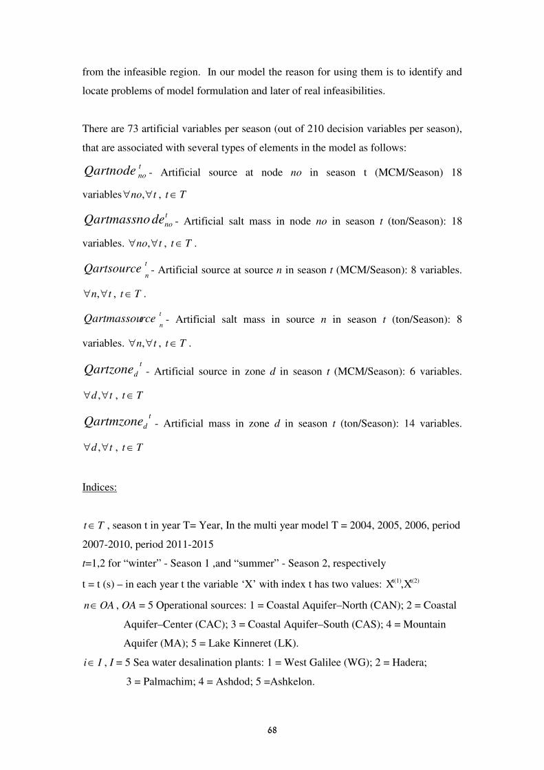
68
from the infeasible region. In our model the reason for using them is to identify and
locate problems of model formulation and later of real infeasibilities.
There are 73 artificial variables per season (out of 210 decision variables per season),
that are associated with several types of elements in the model as follows:
t
noQartnode - Artificial source at node no in season t (MCM/Season) 18
variables tno ∀∀ , , Tt ∈
t
nodeQartmassno - Artificial salt mass in node no in season t (ton/Season): 18
variables. tno ∀∀ , , Tt ∈ .
t
nQartsource - Artificial source at source n in season t (MCM/Season): 8 variables.
tn ∀∀ , , Tt ∈ .
t
nrceQartmassou - Artificial salt mass in source n in season t (ton/Season): 8
variables. tn ∀∀ , , Tt ∈ .
t
dQartzone - Artificial source in zone d in season t (MCM/Season): 6 variables.
td ∀∀ , , Tt ∈
t
dQartmzone - Artificial mass in zone d in season t (ton/Season): 14 variables.
td ∀∀ , , Tt ∈
Indices:
Tt ∈ , season t in year T= Year, In the multi year model T = 2004, 2005, 2006, period
2007-2010, period 2011-2015
t=1,2 for “winter” - Season 1 ,and “summer” - Season 2, respectively
t = t (s) – in each year t the variable ‘X’ with index t has two values: X,X t(2)t(1)
OAn∈ , OA = 5 Operational sources: 1 = Coastal Aquifer–North (CAN); 2 = Coastal
Aquifer–Center (CAC); 3 = Coastal Aquifer–South (CAS); 4 = Mountain
Aquifer (MA); 5 = Lake Kinneret (LK).
Ii∈ , I = 5 Sea water desalination plants: 1 = West Galilee (WG); 2 = Hadera;
3 = Palmachim; 4 = Ashdod; 5 =Ashkelon.

69
FASf ∈ , FAS= 5 Fixed Artificial Sources, 3 Brackish Water Desalination Plants
(BWDP), 2 Import Intakes (Im)
BDWb∈ , BWD = 3 Brackish Water Desalination Plants:
1 = BWD-Hof Carmel ; 2=BWD-Gat ; 3= BWD – Mishor Yeruham (MY)
Im∈im , Im=2 Import Intakes: 1. Import Hadera; 2. Import Ashkelon.
Dd ∈ , D = 14 Demand Zones: 1 = WG– Kishon; 2 = Hof–Carmel;
3 = Pardes-Hana; 4 = Yosh–North; 5 = Sharon; 6 = Gush-Dan; 7 = Modi'in;
8 = Shiflat Lod; 9 = Shiflat Yehuda North; 10 = Jerusalem;
11 = Shiflat Yehuda South; 12= Lachish; 13 = Ashkelon–Gvaram;
14 =Negev.
Nodesno∈ =18 nodes on the conveyance system. The main nodes are: 1 = Kfar
Yehoshua (KY); 2 = Menashe; 3= Mezer; 4 =Rosh–Hayin; 5 =
Achisemech; 6 = Hulda; 7 = Zohar. The rest: 8-18 = points on the
conveyance system
Llf ∈∈ , L – all pipes in the model.
4.4 Constraints
The 78 constraints per season represent groups of constraints.
4.4.1 Hydrological Constraints
Lake Kinneret (LK) is a surface reservoir, while the other natural sources are aquifers;
however the hydrological constraints in the model refer to all sources as “cells” of
water with different characteristics. Therefore, the term “aquifer” is sometimes used
also for LK in defining the mathematical formulation.
The difference between the replenishment from all sources and the water usage from
an aquifer (water balance) is equal to the change in the aquifer volume during the
season. The mathematical definition of that principal is:
(4.1) )( 1−−⋅=∆
∆=−∑∑ t
n
t
nn
nt
n
t
n hhSAT
VQoutQin tn ∀∀ , , Tt ∈ , OAn∈
There are 5 constraints of this type, one for each source.

70
The mass balance for the quality component (salinity) in each source is represented by
the non-linear equation:
(4.2) ( )∑ ∑ −− ⋅−⋅⋅=∆
∆+
∆
∆=
∆
∆=− 11 t
n
t
n
t
n
t
nn
n
n
nnt
n
t
n
t
n
t
n hChCSAT
CV
T
VC
T
CVQoutCoutQoutCin
tn ∀∀ , , Tt ∈ , OAn∈
To represent a "mixing volume" in the aquifer, which allows mixing to occur in part
of the aquifer thickness, a coefficient 10 ≤< nhmix is defined, such that when
1=nhmix dilution occurs in the entire thickness (depth) of the aquifer. This modifies
the preceding equation as follows:
(4.3) ( )∑ ∑ −− ⋅−⋅⋅⋅=∆
∆+
∆
∆=
∆
∆=− 11 t
n
t
n
t
n
t
nnn
nnnt
n
t
n
t
n
t
n hChChmixSAT
CV
T
VC
T
CVQCoutQinCin
tn ∀∀ , , Tt ∈ , OAn∈
Where:
t
nQin - Recharge into n in season t (MCM).
t
nQout - Extraction from aquifer n in season t (MCM).
T
Vn
∆
∆- Change in water volume of aquifer n during the period T∆ (MCM/Season).
nSA - Storativity of aquifer n (between 0 and 1 MCM /m).
1,
−tn
t
n hh - Average water level in aquifer n (above the bottom) in season t and t-1,
respectively (m).
t
nCin - Average salinity of the replenishment of the aquifer (mg Cl-/liter).
t
nCout - Average salinity of the water extracted form the aquifer (mg Cl-/liter).
T
CVn
∆
∆- The change of mass in aquifer n cell during time period T∆ (Tons of Cl
-
/Season).
1−tn
t
nCC - The average water salinity in aquifer n in seasons t and t-1 respectively
(mg/liter).
Notes:
� Salinity in Lake Kinneret is constant. Therefore there are only 4 constraints of
type (4.3).

71
� Both sides of equation (4.3) express the change in total mass of salts per season.
An example for the mass balance is given for the Central Coastal Aquifer:
(4.4) ( )
( )11 −−
→
⋅−⋅⋅⋅
=+−⋅⋅⋅∆⋅−⋅−⋅ ∑∑t
cc
t
CC
t
cc
t
CCCC
t
cc
tt
CC
t
cc
p
tt
CC
r
t
r
t
r
hChChmixSAc
QartmasshspillhccCkdirTKccQnCQC
t∀ , Rr ∈ Tt ∈ , OAn∈
Where:
t
rQ - Natural replenishment and recharge of water from sources and pipes r=1....R
(MCM/Season), each having its own salinity.
t
rC - The salinity of water source r=1...R (mg Cl-/liter).
tQn - The production from aquifer cell n (MCM/Season)
t
CCC - The average salinity in the Central Coastal Aquifer (CCA) (mg Cl-/liter).
CCK - The spill coefficient from CCA to the sea (m2/day)
T∆ - The number of days per season (day)
tCChspill - Spill level above the bottom of the aquifer cell (m).
thcc - Water level in CCA (m).
CChmix - The thickness of the mixing volume in CCA (m).
t
ccQartmass - Artificial mass source (MCM/Season) – used to guarantee mathematical
feasibility; is given a large penalty coefficient in the objective function.
→t
cckdir - A direction coefficient that takes on the value 0 or 1 according to the sign of
the expression ( )hspillhcc t − , so as to zero out the term if the water level is below the
spill level. To avoid an “If statement” which is a non-smooth function, the value of
the direction coefficient tdirk is determined by a "direction equation" and the spill
value by a "smoothing function" (Cohen et al, 2000a), defined by the flowing
expressions.

72
(4.5)
<<=
>>==
++
=0x0
0x1
)x(-exp)xexp(
)xexp(-*0)x(exp*1**
**
when
when
kk
kkdirk
t
Where the spill to the sea given by:
(4.6) x = ( )t
cc
t
CCCC
t
sean hspillhkQ −⋅=−
With a large enough value of k, the expression (4.5) takes on the value 1 if the water
level in the aquifer is above the spill level, and is 0 otherwise, in which case there is
no spill. The actual flow to the sea is given by a relaxation function:
(4.7) ( )( )1*
2
* ±≈+
==
−
−−
εt
sean
t
t
sean
Q
QXQ sean
310
100
−=
=
ε
k
*t
seanQ − rises from 0 at 0=−t
seanQ and tends to 1 quickly as t
seanQ − increases.
The value of k is large enough to drive the negative exponential to zero, while the
small value ε is used to avoid division by zero.
When - tdirk tends to 1 the water / mass loss for the year T in aquifer n is computed
When - tdirk tends to 0 the water / mass loss for the year T in aquifer n is zero.
Note:
• k ,ε determines the of "softness" for the transition from one direction to the
other.
• At his stage, the coefficient tdirk is calculated yearly (according to the value
of t
seanQ − in the winter due to simplification considerations in the multi year
model)
• As a result of these definitions the direction indicator kdir takes on the
following values:

73
0,1,0
1,1,0
*
*
⇒→−⇒→<<
⇒→⇒→>>
kdirXx
kdirXx
Flow Direction Coefficient (kdir)
k=100, epsilon = 0.001
-1.00
-0.50
0.00
0.50
1.00
-100 -75 -50 -25 0 25 50 75 100
Flow range (MCM)
kdir, k=100 Q*
Figure 4.2: Flow Direction Coefficient.
Flow Direction Coefficient (kdir)
k=100, epsilon = 0.001
-1.00
-0.50
0.00
0.50
1.00
-1 -0.75 -0.5 -0.25 0 0.25 0.5 0.75 1
Flow range (MCM)
kdir, k=100 kdir, k=1
Figure 4.3: Sensitivity of the approximation with respect to the coefficient k.
4.4.1.1 Water Level Constraints
(4.8) t
n
t
n
t
n hhh maxmin ≤≤ tn ∀∀ , , Tt ∈ , OAn ∈
There are 5 constraints of this type for each season.
Where:
t
nh min - Minimum seasonal required level in aquifer n (m)
t
nh - Average water level in aquifer n in season t (m)

74
t
nh max - Maximum seasonal allowed level in aquifer n (M)
4.4.1.2 Aquifer Salinity Constraints
(4.9) t
n
t
n
t
n CCC maxmin ≤≤ tn ∀∀ , , Tt ∈ , 4...1∈n
t
nC min - Minimum seasonal average salinity required in aquifer n in season t (mg
Cl-/liter).
t
nC - Average concentration in aquifer n in season t (mg Cl-/liter).
t
nC max - Maximum seasonal average concentration allowed in aquifer n in season
t (mg Cl-/liter).
4.4.1.3 Spills in Lake Kinneret
Spills from Lake Kinneret are decision variables, which satisfy:
(4.10) ttt KinspillKinspillKinspill maxmin ≤≤ t∀ , Tt ∈
Notes:
• There is one constraint per season (part of the UB and the LB constraints).
• The UB and LB could be changed each season, but were fixed in this version
of the model.
4.4.2 Demand
4.4.2.1 Minimum Demand in Consumer Zones
The demand constraint at zone d is defined as:
(4.11) t
d
t
d
l
indt
DDefQ ≥+∑=1
d∀ Dd ∈ , t∀ Tt ∈
There are 14 constraints of this type for each season.
Where:

75
indtQ - The total amount of water supplied to zone d in season t from all pipes
connected to the demand zone (MCM/Season)
t
dD - The demand for water in zone d in season t (MCM/Season).
t
dDef - The deficit of water resulting in zone d (MCM/Season).
4.4.2.2 Prescribed Quality of the water supplied to Consumer Zones
The weighted average salinity in the water supplied to demand zone d in season t.
(4.12) ∑
∑−
− ⋅=
t
dl
t
l
t
dlt
dQ
CQC d∀ Dd ∈ , l∀ dll −∈ , t∀ Tt ∈
Must be below the maximum allowed value
(4.13) t
d
t
d CpsC max≤
There are 14 constraints from that type.
Where:
t
dC - The weighted average salinity supplied to zone d in season t (mg Cl-/liter).
t
dCps max - The maximum weighted average salinity allowed in zone d in season t
(mg Cl-/liter).
4.4.3 Conveyance System
4.4.3.1 Conveyance Capacity
(4.14) t
l
t
l QconQ max0 ≤≤
There are 82 constraints of this type per season.
Where:
t
lQ - The seasonal quantity that flows in pipe l (MCM/Season).
t
lQcon max - The installed conveyance capacity of pipe l (MCM/Season).
Note:
• Development plans of pipe capacities are expressed by changing t
lQcon max .

76
4.4.3.2 Quantity Conservation
(4.15) ∑∑=
−−=
− =+u
out
t
outno
t
noin
l
in
t
noin QaQ11
l∀ inl ∈ , u∀ outu ∈ , no∀ nodesno ∈ , t∀ Tt ∈
t
noina − - Artificial variable
4.4.3.3 Mass Conservation
(4.16) ∑∑=
−−=
−− ⋅=+⋅u
out
t
not
outno
t
noin
l
in
t
noin
t
noin CQmaCQ11
l∀ inl ∈ , u∀ outu ∈ , no∀ nodesno ∈ , t∀ Tt ∈
There are 21 constraints of each type per season.
Where:
ul, - Pipes.
no – node in the supply system.
in - All pipes that convey water into node no.
out - All pipes that convey water out of node no.
nodes – All nodes of the supply system.
∑=
−
l
in
t
noinQ1
- The sum of water from all pipes that convey water to node no in season t
(MCM).
∑=
−
u
out
t
outnoQ1
- The sum of water from all pipes that convey water out of node no in
season t (MCM).
t
noina − - Artificial variable (water - MCM).
t
noinC − - Water quality in pipe in-no (mg Cl-/liter).
t
noC - Weighted average water salinity computed at node no (mg Cl-/liter).
t
inma - Artificial variable (mass - Ton).
The salinity of the water supplied to demand zones is controlled, by placing upper
and/or lower bounds on salinity at the nodes:

77
(4.17) t
no
t
not
no CCC maxmin ≤≤ no∀ nodesno ∈ , t∀ Tt ∈
4.4.3.4 Desalination Capacity
(4.18) t
i
t
i
t
i desQdesdes maxmin ≤≤ i∀ desi ∈ , t∀ Tt ∈
(4.19) t
i
t
i
t
i QdesdesQdesshut −= max i∀ desi ∈ , t∀ Tt ∈
Where :
des - Seawater desalination plants.
t
iQdes - Quantity of water desalinized in plant i in season t (MCM/Season).
t
ides min - Minimum operational capacity in plant i (MCM/Season).
t
ides max - Maximum operational capacity in plant i (MCM/Season).
t
iQdesshut - Operational shutdown of the desalination plant i in season t
(MCM/Season).
Notes:
• Usually 0min =t
ides and =t
ides max installed capacity of plant i.
• The value t
ides max can be changed with time, to express the desalination
development policy.
There are 5 constraints of this type per season, one for each SWD plant.
4.4.3.5 Desalinated Water Quality
(4.20) ( )
10000
10000 t
ii
t
i
RRCnCdes
−⋅= i∀ desi ∈ , t∀ Tt ∈
(4.21) t
i
t
i
t
i RRRRRR maxmin ≤≤ i∀ desi ∈ , t∀ Tt ∈
Where:

78
t
iCdes - Water salinity in the outlet of desalination plant i in season t (mg Cl-/liter).
iCn - The salinity in source n of plant i - mg Cl-/liter. In this model it refers to the
Mediterranean Sea salinity, which is 27,000 mg Cl-/liter.
t
iRR - Percentage removal by plant i in season t (converted from % to the range 0-
10,000, to avoid scaling difficulties); it is a decision variable.
iRR min - Minimum RR in plant i (0-10,000)
iRR max - Maximum RR in plant i (0-10,000)
There are 5 constraints from that type per season, one for each desalination plant.
Note:
• In the current version of the model t
iRR is determined according to the first
season of the first year, but is subject to all constraints of all subsequent years
due to simplification of the multi-year model. It can be explained as the
development plan needed (for salinity removal) to be implemented in the first
year of the model in order to comply with demand in the future constraints as
well.
• The prescribed range for the RR in the current model is 9980-10000.
4.4.4 State Variables
The state variables are the water levels ( t
nh ) and salinities in the aquifers ( t
nC )
They are the initial values for each season and each year. They function as
continuity variables between the years and the season and represent the “memory”
of the water system over time. For the first year and first season the water level and the water
salinity is entered by the user.
In order to compute the initial level at the beginning of the FRY we multiply the
last year change of the state variable by the number of the years (e.g. 2-5) till the
start of the FRY in the representative period. We add the delta computed to the
previous value of the state variable to get the final FRY initial value. The
calculation can be computed by the expression:

79
(4.22) ( )11)(
−− −⋅∆+= t
n
t
n
t
n
t
n XXTXTX
t
nX∀ t
n
t
n
t
n XCh ∈, , t∀ Tt ∈
Where:
T – Final year of the FRY
T∆ - The number of years between the beginning of FRY and the last computed year
in the model
)(TXt
n - State variable of natural aquifer n in season t - salinity mg Cl-/liter or water
level (m).
Note:
• See figure 4.1 for the extrapolation made in the multi- year model.
4.4.5 Non Negative Variables
All decision variables are Non Negative.
tX≤0
4.5 Objective Function
The objective of the multi-year model is to minimize the total cost of operation over
the planning horizon, which is made of 3 consecutive years and 2 FRYs in the future,
a total of 10 seasonal time periods. The components of the (non-linear) objective
function are:
a. Operational cost of pumping and recharge.
b. Operational cost of conveyance.
c. Cost of regional deficits.
d. Operational cost of desalination plants.
e. Cost (penalty) for not using the full capacity of desalination plants.
f. Cost of spills from the Kinneret (loss of water).
g. Extraction levy from the sources.
h. Penalty on artificial variables (this term becomes zero when a feasible solution
is attained).

80
(4.23) ∑
∑
∑∑
∑
∑∑
=
=
==
=
=
+
⋅+⋅+⋅
+
+
+⋅+⋅
=
⋅⋅
T
tt
tS
AV
j
ts
j
ttstD
d
ts
d
ts
d
des
i
ts
i
t
i
ts
i
t
i
OA
n
ts
nl
ts
n
ts
n
ts
l
l
ts
l
r
arfarKinspillCkinspilldefCdef
QdesshutCdesshutQdesCdes
QhELQCE
MinZ
)t
i,E
t(RR
1
2
1)(
1
,,
1
,,
1
,,
1
,
,
,,,,
)1(
varvar
)(
i∀ desi ∈ , t∀ Tt ∈ d∀ Dd ∈ , j∀ avj ∈ , )(tS∀
)(tS - is the specific season (1 winter, 2 summer) of a year t.
The objective function is non-linear in two terms: the extraction levy )( nnL hE and the
salinity removal cost at the desalination plants - )t
iE,
t(RR
t
iCdes .
The present value of the objective function calculates the Net Present Value (NPV) of
the operational cost by using a discount rate on a series of yearly operational costs in
the future:
(4.24) ∑= +
=T
tt
t
r
valuestrNPV
1 )1(),(
r – Annual interest rate.
t - years
Where:
Z - The objective function value - million US $.
tKinspill - The amount of spills in Kinneret in season t (MCM/Season).
CKinspill -The cost of spills from the Kinneret ( )3$
m.
)t
iE,
t
i(RR
t
iCdes - Operational cost of desalination plant i, which includes capital
recovery, energy, maintenance and the percentage removal ( )3$
m.
t
dCdef - Deficit cost in region d in season t ( )3$
m.
varfar - Artificial Variables (AV) cost ( )3$
m.

81
4.5.1 Definition of the Conveyance Cost
(4.25) t
ll
t
l ECECE ⋅= t∀ Tt ∈ l∀ Ll ∈
(4.26) 736.0200
)(
⋅
∆+⋅∆+∆=
t
plTt
l
HLHHE t∀ Tt ∈ l∀ Ll ∈
tCE - Cost of supply (pumping and transporting) ( )3$ m .
lE - Energy consumption ( )3mKw .
tEC - Energy cost in season t ( )Kw$
TH∆ - Topographic lift (m).
lH∆ - Hydraulic energy loss ( ooo )
L - Length of pipe (km)
t
pH∆ - Supply head required (m)
Note: The coefficients 200 is derived from units conversion, where 1 Hp = 0.736 Kw
4.5.2 Extraction Levy
(4.27)
( ) t
n
n
t
nnt
n MaxELH
hHEL ⋅
−−=
int
int1
n∀ Nn ∈ t∀ Tt ∈
(4.28) t
n
t
n
t
n hhH minmaxint −= n∀ Nn ∈ t∀ Tt ∈
(4.29) t
n
t
n
t
n hhh −= max n∀ Nn ∈ t∀ Tt ∈
Where:
t
nEL - Extraction Levy from aquifer n in season t ($/m3)
t
nMaxEL - Maximum Extraction Levy on aquifer n in season t ($/m3)
t
nH int - Operational range in aquifer n in season t (m)
t
nh - Unsaturated thickness in aquifer n in season t (m)
t
nh - Water level in aquifer n in season t (m)

82
(4.30)
⇒
⇒
=
n
t
n
t
n
n
t
n
t
n
t
n
hhEL
hhMaxEL
EL
max
min
n∀ Nn ∈ t∀ Tt ∈
Figure 4.4: Definition sketch for the Extraction Levy
Water Level
No flow below this level
hmin
hmax
Flows & Spills
t
nh
t
nh
t
nH int
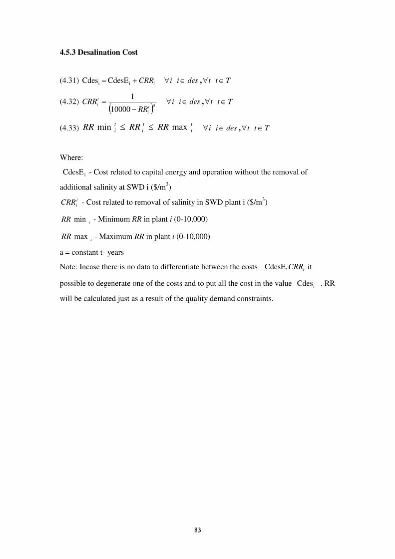
83
4.5.3 Desalination Cost
(4.31) iCRR+= ii CdesE Cdes i∀ desi ∈ , t∀ Tt ∈
(4.32) ( )at
i
t
i
RRCRR
−=
10000
1 i∀ desi ∈ , t∀ Tt ∈
(4.33) t
i
t
i
t
i RRRRRR maxmin ≤≤ i∀ desi ∈ , t∀ Tt ∈
Where:
iCdesE - Cost related to capital energy and operation without the removal of
additional salinity at SWD i ($/m3)
t
iCRR - Cost related to removal of salinity in SWD plant i ($/m3)
iRR min - Minimum RR in plant i (0-10,000)
iRR max - Maximum RR in plant i (0-10,000)
a = constant t- years
Note: Incase there is no data to differentiate between the costs iCRR,CdesE it
possible to degenerate one of the costs and to put all the cost in the value Cdesi . RR
will be calculated just as a result of the quality demand constraints.

84
5. Examples of the Model’s Results
5.1 Introduction
In this chapter some of the model's results will be presented and analyzed. The results
are presented in two sections:
1. Results for one year runs (two seasons), using the annual model.
2. Results for long-term runs (3 successive years and two FRYs to represent two
future periods of several years each) – using the multi–year model.
The results are presented in flow charts and in tables. These are designed as
‘management reports’ in the sense that the information has been condensed into
formats that should be easy to comprehend. There is a color schematic of the entire
system, upon which the season’s results are displayed. It depicts the main components
(detailed in section 4.3, Figure 3.1) of the national water system: desalination plants,
natural sources, consumption zones and the main pipes of the conveyance system. For
each pipe there is an arrow which indicates the direction of flow, and there is a pair of
numbers which give the model’s solution: salinity (mg Cl-/liter) on top (in red) and
quantity (MCM/Season) below (in black). Each main node in the supply system is
numbered and represented by a red circle or box with the node’s name inside. At the
top of each source there a pair of numbers: the average water level per season (m-
ASL – in blue) - and the average salinity per season (mg Cl-/liter – in red).
The description of model’s results both for the annual model and the multi year model
will be presented in this chapter where the main focus will be analyzing the runs’
results. General conclusions and strategic conclusions based on these runs and future
development needed as a result - will be presented in the next chapters.
5.2 Results of the Annual Model
5.2.1 Base Run
The main information for the Base Run (BR) is:
a. Time horizon and time units
One year with two seasons - season 1, “Winter” ~ 275 days, season 2 “Summer “ ~
90 days.

85
b. Development program:
1. Desalination: no sea water desalination available. Most of the supply is from the
natural sources, supplemented by 13 MCM/Year of brackish water desalination.
2. Conveyance System: a few lines of the full model where eliminated: line 11-6
(from node 6 (Hulda) to node 11– in both directions), MA (Mountain Aquifer water
source) to Yosh-N (consumption zone), 10- CC (Recharge from node 10 to the Costal
Aquifer Center), TTA – Mod (from Rosh Ha’Ain to Modi'in). These assumptions are
made in order to represent the “current” development phase of the system better and
to simplify the runs at this stage.
c. Sources management policy:
Extraction levy (‘Hetel Hafaka’): the levies reflect the current order of using the
sources first from Lake Kinneret (max levy=0 US$/m3), next from the Mountain
Aquifer (max levy=0.05 US$/m3), and finally from the Coastal Aquifer (max
levy=0.13 US$/m3).
There are no set of targets (constraints values) on water level and water salinity in the
end of the summer (season 2 – the end of the annual run).
d. Demand management policy:
The full demand should be supplied. The price of water shortage is high enough to
prevent shortages (the deficit cost is two orders of magnitude higher than the average
water supply cost).
e. Quality management policy:
1. The max salinity prescribed for supply to demand zones is 400 mg Cl-/liter.
2. The salinity of Lake Kinneret is 250 mg Cl-/liter (constant).
f. Replenishment:
1. The CA annual replenishment has two “active” components (out of three possible
in the model): replenishment from reclaimed wastewater used for irrigation (~ 50
MCM/Year and 350 mg Cl-/liter) and replenishment from annual precipitation (250
MCM/Year and 250 mg Cl-/liter which include the salts which are “pushed” from the
unsaturated zone into the groundwater).
2. The MA annual replenishment has two components: replenishment from reclaimed
wastewater used for irrigation (~ 20 MCM/Year and 350 mg Cl-/liter) and

86
replenishment from annual precipitation (360 MCM/Year and 140 mg Cl-/liter which
include the salts which are “pushed” from the unsaturated zone into the groundwater).
g. Initial conditions: are summarized in Table 5.1.
Note: Artificial variables are not expected to remain in the solution, since the
introduction of penalties for not meeting demands makes it possible to find a feasible
solution.
Table 5.1: Initial Conditions for the Annual Base Run.
No. Source
Name
Range of allowed
change
of water level
Initial Water
level
above bottom of
base line
Range of
allowed
change
of salinity
Initial Water
Quality
(Salinity)
[m ASL] [m ASL] [mg Cl-/liter] [mg Cl
-/liter]
1 Lake Kinneret -208.9 - -213 - 211.9 250* 250
2 Coastal Aquifer
– North (CN) +30 - -10 +3.5 250-250 150
3 Coastal Aquifer
– Center (CC) +10 - -10 +3.5 150-250 150
4 Coastal Aquifer
– South (CS) +30 - -10 +2 150-250 150
5 Mountain
Aquifer (MA) +22 - +12 +15 140-250 140
* Constant

87
5.2.2 Scenarios Description
The scenarios are presented in Table 5.2.
Table 5.2: Annual Model - Scenarios List.
No Scenario’s Name Scenario’s Description
1 Base Run (BR) Two seasons, no desalination, initial conditions presented in
Table 5.1
2 BR+1m in the Mountain
Aquifer
Same as BR + a constraint of level above + 1m in the Mountain
Aquifer (MA) at the end of the 2nd
season.
3
BR +
150 MCM/Year
in Lake Kinneret Basin
Same as the BR + the consumption in the Lake Kinneret Basin
(LKB) was increased by 150 MCM/Year.
4 BR +
100 MCM/Year Negev
Same as BR + the consumption in the Negev zone was
increased by 100 MCM/Year.
5
BR +150 mg Cl-/liter to
Gush–Dan +
45 Des-Pal
Same as the BR + a constraint on the maximum salinity of 150
mg Cl-/liter in the second season (instead of the original 400
mg Cl-/liter) was imposed on the supply to Gush Dan. A sea
water desalination plant was installed in Palmachim with a
capacity of 45 MCM/Year.
6
BR +150 mg Cl- in
Gush–Dan +
45 Des Pal +
quality limit at KY
Same as Scenario 5 + minimum salinity was imposed at ‘Kfar
Yehusha’ (KY, Node 1) of minimum 250 mg Cl-/liter
5.2.3 Analysis of the Results
The main results of these scenarios are summarized in Table 5.3 and in Figures 5.5-
5.17. Each figure contains the main seasonal values placed on the model’s topology.
Description and analysis of the results are presented in the following section.
Scenario 1: Base Run (BR) – Figure 5.1-5.2
There is no deficit. The difference between the total replenishment and demand (95
MCM/Year, Table 5.3) is supplied from storage in natural sources and from the

88
existing desalination plants of brackish water (13 MCM/Year). There are no sea water
desalination plants.
At the end of the year there is a rise in water table in Lake Kinneret (LK), (+0.23 m)
and in the North Coastal Aquifer (NCA)-(+0.13 m). In the rest of the natural water
sources there is a decline in the water levels. The Mountain Aquifer (MA) was
completely depleted and reached its ‘red line’ (+12m ASL). The salinity of all
aquifers (in all cells) deteriorated by the end of the one year run. The salinity of the
MA was raised by 0.53 mg Cl-/liter and in CA by 1.26 mg Cl
-/liter. In the CA the
deterioration in quality is higher which is associated with the fact that there is more
intensive reclamation above the aquifer and salinity of replenishment from
precipitation is higher.
The objective function (OF) value is 100.1 MUS$/Year. The only “active”
components of the OF are conveyance cost (73%) and extraction levies (27%).
Scenario 2: BR + 1m in the Mountain Aquifer- Figure 5.3-5.4
The water table in MA at the end of the 2nd
season is prescribed to be 1m above the
“red line”. The water level result is as was expected (+13 ASL – 1 m above the + 12
ASL level in BR). The reduction in the extraction of water from MA was
compensated mainly by extracting water from LK. The OF went up by only 2.8
MUS$/ Year. The active components of the OF are the same as in the BR.
The addition in conveyance costs (+5.9 MUS$/Year) is explained by increasing
conveyance from a more expensive source (because of the addition of transportation
length) while this extra expense was compensated by a lower extraction levy (-3
MUS$/ Year) since the extraction levy in LK is 0.
Scenario 3: BR + 150 MCM/Y in the Lake Kinneret Basin - Figure 5.5-5.6
The increase in consumption in the Lake Kinneret Basin (LKB) by 150 MCM/Year
turned out to be a “local change” considering the results of the whole water system. In
comparison with the BR the OF value did not change. The main change was in the
water level in LK. In the BR, the water level in LK at the end of the run (2nd
season)
was 0.89 m higher than in this run (0.23-(-0.67)). The product of the LK storativity
(=1, since it is a lake) times the water level change (0.89m) and the area of the
Kinneret (167 km2) provides the additional demand.

89
There was no extraction levy on the increased demand (it is considered ‘local
production’); therefore this component in the OF did not change and therefore the
total value of the OF did not change.
Scenario 4: BR + 100 MCM/Y to the Negev- Figure 5.7-5.8
In this run the OF had another ‘active’ component which is the Deficit Cost. The local
source (MA) of the Negev demand Zone was fully utilized and was depleted again.
The consumption in the Negev was increased by 100 MCM/Year but there is a
remaining deficit of 6.4 MCM (all in the 2nd
season) as a result of the limitation on the
conveyance capacity in the second season from Zohar (node 7) to the Negev demand
zone. In the first season the conveyance constraint to the Negev was not binding and
the addition of consumption caused the conveyance cost component in the OF to rise
from 47.6 MUS$/Season to 59.2 MUS$/Season. In the 2nd
season the limitation in
capacity and the relatively high cost of deficit caused the OF to peak up to 436
(MUS$/Year).
Scenario 5: BR + 150 mg Cl-/liter to Gush Dan + 45 MCM/Year Desalination in
the Palmachim Plant - Figure 5.9-5.10
The maximum (weighted average) salinity allowed for supply to Gush Dan (GD) in
the 2nd
season was reduced from 400 mg Cl-/liter in the BR to 150 mg Cl
-/liter. A
SWD plant with an installed capacity of 45 MCM/Year was installed in Palmachim. It
was expected that most water will be supplied from the SWD plant due to the quality
restriction and the relatively high initial level of salinity in the aquifers (according to
the Base Run there is no need for desalination due to the wide (non-restrictive) quality
constraints and sufficient water in terms of water quantity).
The SWD plant worked but added only 5.5 MCM (out of the 45 MCM/Year installed)
in the 2nd
season (18 MCM desalinated in total). The range of salinity in the outlet of
the SWD was confined to the range of 0 mg Cl-/liter (RR = 100%) to 50 mg Cl
-/liter
(RR = 99.80%) from origin sea water salinity of 27,000 mg Cl-/ li. The resulting
salinity in the outlet of the desalination plant was 34.4 mg Cl-/liter (R.R. = 99.87%).
The model met the maximum weighted average salinity constraint in Gush Dan (in
the 2nd
season only) by diluting water from Lake Kinneret (LK) in the West Galilee

90
(WG) demand zone. Water from LK is the most saline but cheaper than SWD plant.
The water was supplied to WG through the Kfar Yehoshua (KY) node. The supply
exceeded the demand by 15.65 MCM. The addition of water to WG is explained by
the need to dilute the water before it reaches Gush Dan (GD).
The dilution happened in WG since the water salinity there is low (~50 mg Cl-/liter).
The water that came from LK with 250 mg Cl-/liter came out of the KY node with
224.9 mg Cl-/liter. The water was conveyed south through the National Carrier (NC)
and was diluted again with water from the MA to the level of 170 mg Cl-/liter just
before entering the GD demand zone. Finally, the weighted average of all sources to
GD was 150 mg Cl-/liter - as was prescribed. In the BR the water supplied to GD was
with salinity of 201 mg Cl-/liter.
This run indicates how quality considerations can make a substantial – and somewhat
unexpected – change to the entire production and conveyance scheme.
Scenario 6: BR + 150 mg Cl-/liter to Gush Dan + 45 Desalination in the
Palmachim Plant + Kfar Yehoshua 250 mg Cl-/liter - Figure 5.11-5.12
The dilution of water in WG that occurred in Scenario 5 is in reality not feasible with
the current state of the system. There is no pipe (nor boosters) that can convey the
water from Western Galilee (AG) back to the Kfar Yehoshua (KY) node. To test how
the system would operate without this connection, we can devise two options:
1. Remove the pipe from WG to node KY
2. Adopt a different policy of dilution: eliminate the dilution at node KY by raising its
lower bound on salinity from 0 mg Cl-/liter to 250 mg Cl
-/liter. This makes it possible
to convey LK water further south without mixing at KY.
In this run the second option was adopted. The water was conveyed with higher
salinity in the NC beyond KY, and was not mixed with water from WG. Instead, the
water was diluted further south with water from the Mountain Aquifer (MA). In
addition, the SWD plant in Palmachim supplied more water (+2.9 MCM/Season) with
low salinity to Gush Dan (GD). The Objective Function (OF) was raised by only a
small amount (+0.4 MUS$) as compared to Scenario 5, since there is a tradeoff
between various OF components.

seaso
n 1
seaso
n 2
To
tal
seaso
n 1
seaso
n 2
To
tal
seaso
n 1
seaso
n 2
To
tal
seaso
n 1
seaso
n 2
To
tal
seaso
n 1
seaso
n 2
To
tal
seaso
n 1
seaso
n 2
To
tal
Un
it
1T
ota
l R
ep
len
ish
men
t*1,2
96.2
151.8
1,4
48
1,2
96.2
151.8
1,4
48
1,2
96.2
151.8
1,4
48
1,2
96.2
151.8
1,4
48
1,2
96.2
151.8
1,4
48
1,2
96.2
151.8
1,4
48
2T
ota
l D
em
an
d1,0
02.6
539.9
1,5
43
1,0
02.6
539.9
1,5
43
1,1
00.1
592.4
1,6
93
1,0
66.7
574.4
1,6
41
1,0
02.6
539.9
1,5
43
1,0
02.6
539.9
1,5
43
3W
ate
r S
up
ply
1002.6
539.9
1,5
43
1002.6
539.9
1,5
43
1100.1
592.4
1,6
93
1066.7
568.5
1,6
35
1002.6
555.5
1,5
58
1002.6
539.9
1,5
43
4D
efi
cit
0.0
0.0
00.0
0.0
00.0
0.0
00.0
6.4
60.0
0.0
00.0
0.0
0
5D
esali
nati
on
& A
rtif
icia
l S
ou
rces
6.5
6.5
13
6.5
6.5
13
6.5
6.5
13
6.5
6.5
13
6.5
12.0
18
6.5
14.9
21
6W
ate
r E
xtr
acti
on
918.1
491.4
1,4
10
918.1
491.4
1,4
10
1015.6
543.9
1,5
60
982.1
519.9
1,5
02
918.1
485.9
1,4
04
918.1
483.0
1,4
01
7
K
inn
ere
t409.2
202.7
612
438.9
237.8
677
506.7
255.2
762
486.4
217.4
704
437.8
151.6
589
437.8
154.1
592
8
M
ou
nta
in A
qu
ifer
(MA
)372.4
207.9
580
342.7
170.8
514
372.4
207.9
580
359.3
221.0
580
343.9
236.4
580
343.9
236.4
580
9
C
oasta
l A
qu
ifer
(CA
)136.5
80.8
217
136.5
82.8
219
136.5
80.8
217
136.5
81.6
218
136.5
97.8
234
136.5
92.4
229
10
Wate
r R
ech
arg
e0.0
0.0
00.0
0.0
00.0
0.0
00.0
0.0
00.0
0.0
00.0
0.0
0
11
Flo
ws &
Sp
ills
65.0
20.6
86
65.0
20.5
86
65.0
20.6
86
65.0
20.5
86
65.0
20.1
85
65.0
20.3
85
12
Sto
rag
e C
han
ge
235.0
-402.2
-167
235.0
-402.1
-167
137.5
-454.7
-317
171.0
-430.7
-260
235.0
-396.2
-161
235.0
-393.4
-158
13
Wate
r le
vel
ch
an
ge
14
Kin
nere
t1.2
5-1
.02
0.2
31.0
7-1
.23
-0.1
60.6
7-1
.34
-0.6
70.7
9-1
.11
-0.3
21.0
8-0
.72
0.3
61.0
8-0
.74
0.3
5
15
Mo
un
tain
Aq
uif
er
(MA
)0.0
4-3
.04
-3.0
00.4
8-2
.48
-2.0
00.0
4-3
.04
-3.0
00.2
4-3
.24
-3.0
00.4
7-3
.47
-3.0
00.4
7-3
.47
-3.0
0
16
Co
asta
l A
qu
ifer
(CA
)**
0.1
9-0
.25
-0.0
60.1
9-0
.28
-0.0
90.1
9-0
.25
-0.0
60.1
9-0
.27
-0.0
80.1
9-0
.44
-0.2
50.1
9-0
.38
-0.1
9
17
Qu
ali
ty C
han
ge
18
Mo
un
tain
Aq
uif
er
(MA
)0.3
90.1
30.5
30.3
90.1
30.5
30.3
90.1
30.5
30.3
90.1
30.5
30.3
90.1
30.5
30.3
90.1
30.5
3
19
Co
asta
l A
qu
ifer
(CA
)**
0.9
40.3
11.2
60.9
40.3
11.2
60.9
40.3
11.2
60.9
40.3
11.2
60.9
40.3
11.2
60.9
40.3
11.2
6
20
Ob
jecti
ve F
un
cti
on
***
64.6
35.5
100.1
65.9
37.0
102.9
64.6
35.5
100.1
75.6
360.3
435.9
72.6
44.3
116.9
72.6
44.7
117.3
21
Co
nveyan
ce C
ost
47.6
25.0
72.6
50.3
28.1
78.5
47.6
25.0
72.6
59.2
29.0
88.2
50.2
20.8
71.0
50.2
20.5
70.7
22
Sea W
ate
r D
esali
nati
on
Co
st
0.0
0.0
0.0
0.0
0.0
0.0
0.0
0.0
0.0
0.0
0.0
0.0
0.0
4.3
4.3
0.0
6.5
6.5
23
Kin
nere
t S
pil
l C
ost
0.0
0.0
0.0
0.0
0.0
0.0
0.0
0.0
0.0
0.0
0.0
0.0
0.0
0.0
0.0
0.0
0.0
0.0
24
Dem
an
d Z
on
e's
Defi
cit
e C
ost
0.0
0.0
0.0
0.0
0.0
0.0
0.0
0.0
0.0
0.0
320.0
320.0
0.0
0.0
0.0
0.0
0.0
0.0
25
To
tal
Art
ific
ial
Vari
ab
les C
ost
0.0
0.0
0.0
0.0
0.0
0.0
0.0
0.0
0.0
0.0
0.0
0.0
0.0
0.0
0.0
0.0
0.0
0.0
26
Pro
du
cti
on
Levy
17.0
10.5
27.5
15.6
8.9
24.5
17.0
10.5
27.5
16.4
11.3
27.6
15.6
14.1
29.7
15.6
13.4
29.0
27
Sea W
ate
r D
esali
nati
on
Sh
utd
ow
n C
ost
0.0
0.0
0.0
0.0
0.0
0.0
0.0
0.0
0.0
0.0
0.0
0.0
6.8
5.1
11.9
6.8
4.2
11.0
* I
nclu
din
g r
eple
nis
hm
ent
in W
G &
Hof
Carm
el
** A
vera
ge o
f all 3
cells
*** W
ithout
am
ort
ization
B.R
. +
15
0 m
g C
l- li
Gu
sh
Da
n+
45
de
s P
al
B.R
. +
15
0 m
g C
l- li
Gu
sh
Da
n+
45
de
s
Pa
l+K
Y 2
50
mg
Cl-
56
B.R
. 1
m i
n M
AB
.R.+
15
0 M
CM
LK
BB
.R.+
10
0M
CM
Ne
ge
v
41
2
Sc
en
ari
os
Ta
ble
5.3
: A
nn
ua
l M
od
el -
Ma
in R
es
ult
s
m
mg
Cl- /
li
MU
S$
MC
M
3
Ba
se
Ru
n (
B.R
)
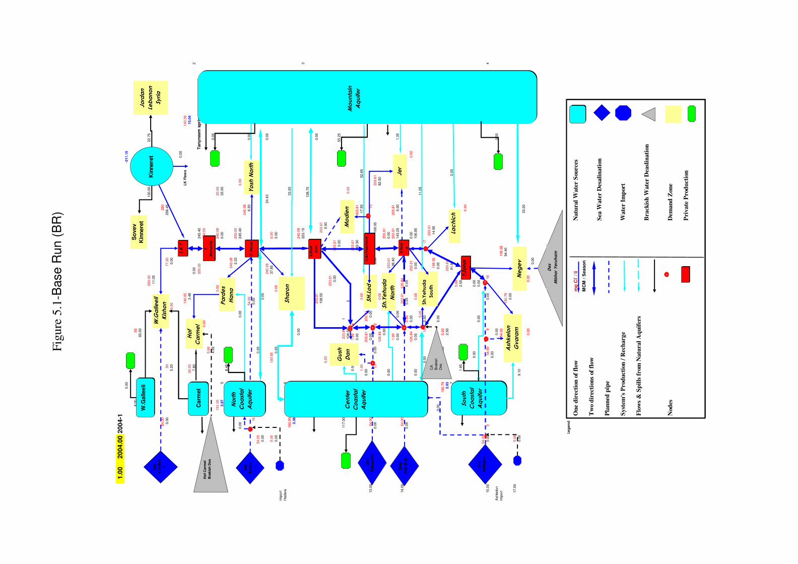
Fig
ure
5.1
-Base R
un (
BR
)
1.0
02
00
4.0
02
00
4-1
0.0
0-2
11.1
5
8.0
050
65.0
0
250.0
0130.0
022.7
5
11.0
5
54.0
0250
0.0
050
77.2
0256.4
5
5.2
00.0
00.0
0
0.0
0
146.9
5L
K F
low
s140.3
9
50.0
03.4
815.0
4
7.8
00.0
02
250.0
0245.4
0T
an
yn
eem
sp
rin
gs
0.0
0250.0
0
5.0
0
4.0
00.0
0
18.0
0151.0
50.0
0240.0
820.0
0
3.9
75
0.0
033.0
0
8.4
5
240.0
8
2.3
3250.0
0
0.0
00.0
0245.4
00.0
0
240.0
8
54.0
06.5
00.0
0
16
0.0
0
54.0
00.0
0
0.0
00.0
0
240.0
824.4
30.0
0
5.0
0193.6
537.8
50.0
0
0.0
00.0
00.0
00.0
0
impo
rt
16
Hadera
6
150.9
933.0
0140.3
9
3.3
815.0
4
0.0
0240.0
8
223.1
53
128.7
0
203.6
10.0
0
108.5
5203.6
1
0.0
00.0
0
203.6
1
0.0
0203.6
1
0.0
055.2
5
117.0
0203.6
11
108.5
52
0.0
0
0.0
01.0
014
203.6
1
0.0
0243.3
0203.6
1
1.0
00.0
017.5
552.6
5
0.0
0203.6
1203.6
1
13.0
054.0
013.0
00.0
00.0
015
0.0
013
0.0
012
0.0
0100.0
5203.6
1
126.8
40.0
082.5
0
0.0
0203.6
1
0.0
0203.6
10.0
0
1.0
036.4
0203.6
1203.6
1
0.0
00.0
0143.2
50.0
01.3
5
14.0
054.0
011
203.6
1126.8
4
0.0
05.0
00.0
00.0
0
126.8
40.0
0203.6
10.0
00.0
0
0.0
00.0
00.0
00.0
0106.8
5
5.0
011.0
5
0.0
010
0.0
017
203.6
1
198.3
514.9
5
0.0
00.0
00.0
0
150.7
919.0
05.0
0
2.0
32.5
0203.6
1
791.9
00.0
0
5.0
0
1.9
52.5
0
0.0
0
0.0
00.0
020.0
0
0.0
00.0
0110.0
0
54.0
0
15.0
00.0
09
54.0
08
0.0
018
4
0.0
0
Ashkelo
n0.0
00.0
0
impo
rt54.0
0198.3
5
150.7
994.4
0
0.0
0
17.0
05.0
0
0.0
09.1
0
33.0
0
0.0
00.0
0
0.0
0
Legend
On
e d
irec
tion
of
flow
mg
Cl- /
liN
atu
ral
Wate
r S
ou
rces
MC
M /
Se
aso
n
Tw
o d
irec
tion
s of
flow
Sea
Wate
r D
esali
nati
on
Pla
nn
ed p
ipe
Syst
em's
Pro
du
ctio
n /
Rec
harg
e W
ate
r Im
port
Flo
ws
& S
pil
ls f
rom
Natu
ral
Aq
uif
ers
Bra
ckis
h W
ate
r D
easl
inati
on
Nod
esD
eman
d Z
on
e
Pri
vate
Pro
du
ctio
n
South
Coastal
Aquifer
W.Galleeli
Kishon
2.Menashe
3. Mezer
4.Rosh �
Hain
7.Zohar
7
Des
W.G
alle
e
li
Pardes
Hana
Des
Had
era
Gush
Dan
Modien
Jer
Des
Ash
kelo
n
Negev
Ashkelon
Gvaram
Des
Palm
ach
im
Des
Ash
do
d
כזמר .ת"יר
Mountain
Aquifer
Jordan
Lebanon
Syria
Yosh North
Ho
f C
arm
el
Bra
kis
h D
es
Carm
el
W.G
alleeli
1.K.Y
Des
Mishor Yeruham
SH.Lod
Sh.Yehuda
North
Lachich
Sh.Yehuda
South
Sharon
5.Achisemech
6.Huld
a
Hof
Carmel
CA
Bra
kis
h
Des
North
Coastal
Aquifer
Center
Coastal
Aquifer
Kin
nere
t
So
vev
Kin
nere
t

Fig
ure
5.2
:Base R
un (
BR
)
2.0
02
00
4.0
02
00
4-2
0.0
0-2
12.1
7
8.0
050
35.0
0
250.0
070.0
012.2
5
5.9
5
54.0
0250
0.0
050
77.2
0120.4
6
2.8
00.0
00.0
0
0.0
0
171.3
9L
K F
low
s140.5
3
50.0
00.0
212.0
0
4.2
00.0
02
250.0
0114.5
1T
an
yn
eem
sp
rin
gs
0.0
0250.0
0
5.0
0
4.0
00.0
0
18.0
0151.3
90.0
0223.6
820.0
0
4.1
05
0.0
010.8
0
4.5
5
223.6
8
6.3
8250.0
0
0.0
00.0
0114.5
10.0
0
223.6
8
54.4
33.5
00.0
0
16
0.0
0
54.0
00.0
0
0.0
00.0
0
223.6
836.2
40.0
0
5.0
0200.1
427.3
50.0
0
0.0
00.0
00.0
00.0
0
impo
rt
16
Hadera
6
151.3
210.8
0140.5
3
3.1
512.0
0
0.0
0223.6
8
113.5
33
42.1
2
201.1
80.0
0
58.4
5201.1
8
0.0
00.0
0
201.1
8
0.0
0201.1
8
0.0
029.7
5
63.0
0201.1
81
58.4
52
0.0
0
0.0
01.0
014
201.1
8
0.0
097.2
0201.1
8
1.0
00.0
09.4
528.3
5
0.0
0201.1
8201.1
8
13.0
054.0
013.0
00.0
00.0
015
0.0
013
0.0
012
0.0
023.2
8201.1
8
73.2
40.0
013.8
3
0.0
0201.1
8
3.7
8201.1
80.0
0
1.0
015.8
2201.1
8201.1
8
0.0
00.0
073.9
20.0
031.3
2
14.0
054.0
011
201.1
873.2
4
0.0
05.0
00.0
00.0
0
73.2
40.0
0201.1
80.0
00.0
0
0.0
00.0
00.0
00.0
058.1
0
5.0
05.9
5
0.0
010
0.0
017
201.1
8
189.6
46.3
2
0.0
00.0
00.0
0
151.0
619.0
05.0
0
1.8
72.5
0201.1
8
751.7
81.7
3
5.0
0
1.0
52.5
0
0.0
0
0.0
03.5
220.0
0
3.5
20.0
0110.0
0
54.0
0
15.0
00.0
09
443.3
58
0.0
018
4
0.0
0
Ashkelo
n0.0
00.0
0
impo
rt1.0
0189.6
4
151.0
657.8
0
0.0
0
17.0
05.0
0
0.0
04.9
0
10.8
0
0.0
00.0
0
0.0
0
Legend
On
e d
irec
tion
of
flow
mg
Cl- /
liN
atu
ral
Wate
r S
ou
rces
MC
M / S
easo
n
Tw
o d
irec
tion
s of
flow
Sea
Wate
r D
esali
nati
on
Pla
nn
ed p
ipe
Syst
em
's P
rod
uct
ion
/ R
ech
arg
e W
ate
r Im
port
Flo
ws
& S
pil
ls f
rom
Natu
ral
Aq
uif
ers
Bra
ckis
h W
ate
r D
easl
inati
on
Nod
esD
eman
d Z
on
e
Pri
vate
Pro
du
ctio
n
South
Coastal
Aquifer
W.Galleeli
Kishon
2.Menashe
3. Mezer
4.Rosh �
Hain
7.Zohar
7
Des
W.G
alle
eli
Pardes
Hana
Des
Had
era
Gush
Dan
Modien
Jer
Des
Ash
kelo
n
Negev
Ashkelon
Gvaram
Des
Palm
ach
im
Des
Ash
do
d
כזמר .ת"יר
Mountain
Aquifer
Jordan
Lebanon
Syria
Yosh North
Ho
f C
arm
el
Bra
kis
h D
es
Carm
el
W.G
alleeli
1.K.Y
Des
Mishor Yeruham
SH.Lod
Sh.Yehuda
North
Lachich
Sh.Yehuda
South
Sharon
5.Achisemech
6.Huld
a
Hof
Carmel
CA
Bra
kis
h
Des
North
Coastal
Aquifer
Center
Coastal
Aquifer
Kin
nere
t
So
vev
Kin
nere
t

Fig
ure
5.3
: B
.R.+
1m
in t
he M
ounta
in A
quifer
1.0
02
00
4.0
02
00
4-1
0.0
0-2
11.3
3
8.0
050
65.0
0
250.0
0130.0
022.7
5
11.0
5
54.0
0250
0.0
050
77.2
0286.1
7
5.2
00.0
00.0
0
0.0
0
147.6
1L
K F
low
s140.3
9
50.0
03.4
815.4
8
7.8
00.0
02
250.0
0275.1
2T
an
yn
eem
sp
rin
gs
0.0
0250.0
0
5.0
0
4.0
00.0
0
18.0
0151.0
50.0
0250.0
020.0
0
3.9
75
0.0
033.0
0
8.4
5
250.0
0
2.3
3250.0
0
0.0
00.0
0275.1
20.0
0
250.0
0
54.0
06.5
00.0
0
16
0.0
0
54.0
00.0
0
0.0
00.0
0
250.0
00.0
00.0
0
5.0
0198.9
537.8
50.0
0
0.0
00.0
00.0
00.0
0
impo
rt
16
Hadera
6
150.9
933.0
0140.3
9
3.3
815.4
8
0.0
0250.0
0
228.4
53
123.4
0
211.5
60.0
0
108.5
5211.5
6
0.0
00.0
0
211.5
6
0.0
0211.5
6
0.0
055.2
5
117.0
0211.5
61
108.5
52
0.0
0
0.0
01.0
014
211.5
6
0.0
0243.3
0211.5
6
1.0
00.0
017.5
552.6
5
0.0
0211.5
6211.5
6
13.0
054.0
013.0
00.0
00.0
015
0.0
013
0.0
012
0.0
0100.0
5211.5
6
126.8
40.0
082.5
0
0.0
0211.5
6
0.0
0211.5
60.0
0
1.0
036.4
0211.5
6211.5
6
0.0
00.0
0143.2
50.0
01.3
5
14.0
054.0
011
211.5
6126.8
4
0.0
05.0
00.0
00.0
0
126.8
40.0
0211.5
60.0
00.0
0
0.0
00.0
00.0
00.0
0106.8
5
5.0
011.0
5
0.0
010
0.0
017
211.5
6
206.0
914.9
5
0.0
00.0
00.0
0
150.7
919.0
05.0
0
2.0
32.5
0211.5
6
791.9
00.0
0
5.0
0
1.9
52.5
0
0.0
0
0.0
00.0
020.0
0
0.0
00.0
0110.0
0
54.0
0
15.0
00.0
09
54.0
08
0.0
018
4
0.0
0
Ashkelo
n0.0
00.0
0
impo
rt54.0
0206.0
9
150.7
994.4
0
0.0
0
17.0
05.0
0
0.0
09.1
0
33.0
0
0.0
00.0
0
0.0
0
Legend
On
e d
irec
tion
of
flow
mg
Cl- /
liN
atu
ral
Wate
r S
ou
rces
MC
M /
Se
aso
n
Tw
o d
irec
tion
s of
flow
Sea
Wate
r D
esali
nati
on
Pla
nn
ed p
ipe
Syst
em's
Pro
du
ctio
n /
Rec
harg
e W
ate
r Im
port
Flo
ws
& S
pil
ls f
rom
Natu
ral
Aq
uif
ers
Bra
ckis
h W
ate
r D
easl
inati
on
Nod
esD
eman
d Z
on
e
Pri
vate
Pro
du
ctio
n
South
Coastal
Aquifer
W.Galleeli
Kishon
2.Menashe
3. Mezer
4.Rosh �
Hain
7.Zohar
7
Des
W.G
alle
e
li
Pardes
Hana
Des
Had
era
Gush
Dan
Modien
Jer
Des
Ash
kelo
n
Negev
Ashkelon
Gvaram
Des
Palm
ach
im
Des
Ash
do
d
כזמר .ת"יר
Mountain
Aquifer
Jordan
Lebanon
Syria
Yosh North
Ho
f C
arm
el
Bra
kis
h D
es
Carm
el
W.G
alleeli
1.K.Y
Des
Mishor Yeruham
SH.Lod
Sh.Yehuda
North
Lachich
Sh.Yehuda
South
Sharon
5.Achis
emech
6.Huld
a
Hof
Carmel
CA
Bra
kis
h
Des
North
Coastal
Aquifer
Center
Coastal
Aquifer
Kin
nere
t
So
vev
Kin
nere
t

Fig
ure
5.4
: B
.R.+
1m
in t
he M
ounta
in A
quifer
2.0
02
00
4.0
02
00
4-2
0.0
0-2
12.5
6
8.0
050
35.0
0
250.0
070.0
012.2
5
5.9
5
54.0
0250
0.0
050
77.2
0155.5
2
2.8
00.0
00.0
0
0.0
0
181.1
6L
K F
low
s140.5
3
50.0
00.0
213.0
0
4.2
00.0
02
250.0
0149.5
7T
an
yn
eem
sp
rin
gs
0.0
0250.0
0
5.0
0
4.0
00.0
0
18.0
0151.3
90.0
0250.0
020.0
0
4.1
05
0.0
010.8
0
4.5
5
250.0
0
6.3
8250.0
0
0.0
00.0
0149.5
70.0
0
250.0
0
54.4
33.5
00.0
0
16
0.0
0
54.0
00.0
0
0.0
00.0
0
250.0
00.0
00.0
0
5.0
0219.0
127.3
50.0
0
0.0
00.0
00.0
00.0
0
impo
rt
16
Hadera
6
151.3
210.8
0140.5
3
3.1
413.0
0
0.0
0250.0
0
112.3
53
42.1
2
220.1
50.0
0
57.2
7220.1
5
0.0
00.0
0
220.1
5
0.0
0220.1
5
0.0
029.7
5
63.0
0220.1
51
57.2
72
0.0
0
1.1
81.0
014
220.1
5
0.0
097.2
0220.1
5
1.0
00.0
09.4
528.3
5
0.0
0220.1
5220.1
5
13.0
054.0
013.0
00.0
00.0
015
0.0
013
0.0
012
0.0
023.2
8220.1
5
81.3
80.0
013.8
3
0.0
0220.1
5
3.7
8220.1
50.0
0
1.0
015.8
2220.1
5220.1
5
0.0
00.0
073.9
20.0
031.3
2
14.0
054.0
011
220.1
581.3
8
0.0
05.0
00.0
00.0
0
81.3
80.0
0220.1
50.0
00.0
0
0.0
00.0
00.0
00.0
058.1
0
5.0
05.9
5
0.0
010
0.0
017
220.1
5
205.6
87.1
2
0.0
00.0
00.0
0
151.0
619.0
05.0
0
1.8
52.5
0220.1
5
750.9
80.9
3
5.0
0
1.0
52.5
0
0.0
0
0.0
04.3
220.0
0
4.3
20.0
0110.0
0
54.0
0
15.0
00.0
09
443.3
58
0.0
018
4
0.0
0
Ashkelo
n0.0
00.0
0
impo
rt1.0
0205.6
8
151.0
657.8
0
0.0
0
17.0
05.0
0
0.0
04.9
0
10.8
0
0.0
00.0
0
0.0
0
Legend
On
e d
irec
tion
of
flow
mg
Cl- /
liN
atu
ral
Wate
r S
ou
rces
MC
M /
Se
aso
n
Tw
o d
irec
tion
s of
flow
Sea
Wate
r D
esali
nati
on
Pla
nn
ed p
ipe
Syst
em's
Pro
du
ctio
n /
Rec
harg
e W
ate
r Im
port
Flo
ws
& S
pil
ls f
rom
Natu
ral
Aq
uif
ers
Bra
ckis
h W
ate
r D
easl
inati
on
Nod
esD
eman
d Z
on
e
Pri
vate
Pro
du
ctio
n
South
Coastal
Aquifer
W.Galleeli
Kishon
2.Menashe
3. Mezer
4.Rosh �
Hain
7.Zohar
7
Des
W.G
alle
e
li
Pardes
Hana
Des
Had
era
Gush
Dan
Modien
Jer
Des
Ash
kelo
n
Negev
Ashkelon
Gvaram
Des
Palm
ach
im
Des
Ash
do
d
כזמר .ת"יר
Mountain
Aquifer
Jordan
Lebanon
Syria
Yosh North
Ho
f C
arm
el
Bra
kis
h D
es
Carm
el
W.G
alleeli
1.K.Y
Des
Mishor Yeruham
SH.Lod
Sh.Yehuda
North
Lachich
Sh.Yehuda
South
Sharon
5.Achis
emech
6.Huld
a
Hof
Carmel
CA
Bra
kis
h
Des
North
Coastal
Aquifer
Center
Coastal
Aquifer
Kin
nere
t
So
vev
Kin
nere
t

Fig
ure
5.5
: B
.R +
150 M
CM
/Year
in t
he L
ake K
innere
t B
asin
1.0
02
00
4.0
02
00
4-1
0.0
0-2
11.7
3
8.0
050
65.0
0
250.0
0227.5
022.7
5
11.0
5
54.0
0250
0.0
050
77.2
0256.4
9
5.2
00.0
00.0
0
0.0
0
146.9
5L
K F
low
s140.3
9
50.0
03.4
815.0
4
7.8
00.0
02
250.0
0245.4
4T
an
yn
eem
sp
rin
gs
0.0
0250.0
0
5.0
0
4.0
00.0
0
18.0
0151.0
50.0
0240.0
920.0
0
3.9
75
0.0
033.0
0
8.4
5
240.0
9
2.3
3250.0
0
0.0
00.0
0245.4
40.0
0
240.0
9
54.0
06.5
00.0
0
16
0.0
0
54.0
00.0
0
0.0
00.0
0
240.0
924.3
90.0
0
5.0
0193.6
637.8
50.0
0
0.0
00.0
00.0
00.0
0
impo
rt
16
Hadera
6
150.9
933.0
0140.3
9
3.3
815.0
4
0.0
0240.0
9
223.1
53
128.7
0
203.6
20.0
0
108.5
5203.6
2
0.0
00.0
0
203.6
2
0.0
0203.6
2
0.0
055.2
5
117.0
0203.6
21
108.5
52
0.0
0
0.0
01.0
014
203.6
2
0.0
0243.3
0203.6
2
1.0
00.0
017.5
552.6
5
0.0
0203.6
2203.6
2
13.0
054.0
013.0
00.0
00.0
015
0.0
013
0.0
012
0.0
0100.0
5203.6
2
126.8
40.0
082.5
0
0.0
0203.6
2
0.0
0203.6
20.0
0
1.0
036.4
0203.6
2203.6
2
0.0
00.0
0143.2
50.0
01.3
5
14.0
054.0
011
203.6
2126.8
4
0.0
05.0
00.0
00.0
0
126.8
40.0
0203.6
20.0
00.0
0
0.0
00.0
00.0
00.0
0106.8
5
5.0
011.0
5
0.0
010
0.0
017
203.6
2
198.3
614.9
5
0.0
00.0
00.0
0
150.7
919.0
05.0
0
2.0
32.5
0203.6
2
791.9
00.0
0
5.0
0
1.9
52.5
0
0.0
0
0.0
00.0
020.0
0
0.0
00.0
0110.0
0
54.0
0
15.0
00.0
09
54.0
08
0.0
018
4
0.0
0
Ashkelo
n0.0
00.0
0
impo
rt54.0
0198.3
6
150.7
994.4
0
0.0
0
17.0
05.0
0
0.0
09.1
0
33.0
0
0.0
00.0
0
0.0
0
Legend
On
e d
irec
tion
of
flow
mg
Cl- /
liN
atu
ral
Wate
r S
ou
rces
MC
M /
Se
aso
n
Tw
o d
irec
tion
s of
flow
Sea
Wate
r D
esali
nati
on
Pla
nn
ed p
ipe
Syst
em's
Pro
du
ctio
n /
Rec
harg
e W
ate
r Im
port
Flo
ws
& S
pil
ls f
rom
Natu
ral
Aq
uif
ers
Bra
ckis
h W
ate
r D
easl
inati
on
Nod
esD
eman
d Z
on
e
Pri
vate
Pro
du
ctio
n
South
Coastal
Aquifer
W.Galleeli
Kishon
2.Menashe
3. Mezer
4.Rosh �
Hain
7.Zohar
7
Des
W.G
alle
e
li
Pardes
Hana
Des
Had
era
Gush
Dan
Modien
Jer
Des
Ash
kelo
n
Negev
Ashkelon
Gvaram
Des
Palm
ach
im
Des
Ash
do
d
כזמר .ת"יר
Mountain
Aquifer
Jordan
Lebanon
Syria
Yosh North
Ho
f C
arm
el
Bra
kis
h D
es
Carm
el
W.G
alleeli
1.K.Y
Des
Mishor Yeruham
SH.Lod
Sh.Yehuda
North
Lachich
Sh.Yehuda
South
Sharon
5.Achis
emech
6.Huld
a
Hof
Carmel
CA
Bra
kis
h
Des
North
Coastal
Aquifer
Center
Coastal
Aquifer
Kin
nere
t
So
vev
Kin
nere
t

Fig
ure
5.6
: B
.R +
150 M
CM
/Year
in t
he L
ake K
innere
t B
asin
2.0
02
00
4.0
02
00
4-2
0.0
0-2
13.0
7
8.0
050
35.0
0
250.0
0122.5
012.2
5
5.9
5
54.0
0250
0.0
050
77.2
0120.4
2
2.8
00.0
00.0
0
0.0
0
171.3
8L
K F
low
s140.5
3
50.0
00.0
212.0
0
4.2
00.0
02
250.0
0114.4
7T
an
yn
eem
sp
rin
gs
0.0
0250.0
0
5.0
0
4.0
00.0
0
18.0
0151.3
90.0
0223.6
520.0
0
4.1
05
0.0
010.8
0
4.5
5
223.6
5
6.3
8250.0
0
0.0
00.0
0114.4
70.0
0
223.6
5
54.4
33.5
00.0
0
16
0.0
0
54.0
00.0
0
0.0
00.0
0
223.6
536.2
80.0
0
5.0
0200.1
227.3
50.0
0
0.0
00.0
00.0
00.0
0
impo
rt
16
Hadera
6
151.3
210.8
0140.5
3
3.1
512.0
0
0.0
0223.6
5
113.5
33
42.1
2
201.1
60.0
0
58.4
5201.1
6
0.0
00.0
0
201.1
6
0.0
0201.1
6
0.0
029.7
5
63.0
0201.1
61
58.4
52
0.0
0
0.0
01.0
014
201.1
6
0.0
097.2
0201.1
6
1.0
00.0
09.4
528.3
5
0.0
0201.1
6201.1
6
13.0
054.0
013.0
00.0
00.0
015
0.0
013
0.0
012
0.0
023.2
8201.1
6
81.3
80.0
013.8
3
0.0
0201.1
6
3.7
8201.1
60.0
0
1.0
015.8
2201.1
6201.1
6
0.0
00.0
073.9
20.0
031.3
2
14.0
054.0
011
201.1
681.3
8
0.0
05.0
00.0
00.0
0
81.3
80.0
0201.1
60.0
00.0
0
0.0
00.0
00.0
00.0
058.1
0
5.0
05.9
5
0.0
010
0.0
017
201.1
6
189.6
26.3
2
0.0
00.0
00.0
0
151.0
619.0
05.0
0
1.8
72.5
0201.1
6
751.7
81.7
3
5.0
0
1.0
52.5
0
0.0
0
0.0
03.5
220.0
0
3.5
20.0
0110.0
0
54.0
0
15.0
00.0
09
443.3
58
0.0
018
4
0.0
0
Ashkelo
n0.0
00.0
0
impo
rt1.0
0189.6
2
151.0
657.8
0
0.0
0
17.0
05.0
0
0.0
04.9
0
10.8
0
0.0
00.0
0
0.0
0
Legend
On
e d
irec
tion
of
flow
mg
Cl- /
liN
atu
ral
Wate
r S
ou
rces
MC
M /
Se
aso
n
Tw
o d
irec
tion
s of
flow
Sea
Wate
r D
esali
nati
on
Pla
nn
ed p
ipe
Syst
em's
Pro
du
ctio
n /
Rec
harg
e W
ate
r Im
port
Flo
ws
& S
pil
ls f
rom
Natu
ral
Aq
uif
ers
Bra
ckis
h W
ate
r D
easl
inati
on
Nod
esD
eman
d Z
on
e
Pri
vate
Pro
du
ctio
n
South
Coastal
Aquifer
W.Galleeli
Kishon
2.Menashe
3. Mezer
4.Rosh �
Hain
7.Zohar
7
Des
W.G
alle
e
li
Pardes
Hana
Des
Had
era
Gush
Dan
Modien
Jer
Des
Ash
kelo
n
Negev
Ashkelon
Gvaram
Des
Palm
ach
im
Des
Ash
do
d
כזמר .ת"יר
Mountain
Aquifer
Jordan
Lebanon
Syria
Yosh North
Ho
f C
arm
el
Bra
kis
h D
es
Carm
el
W.G
alleeli
1.K.Y
Des
Mishor Yeruham
SH.Lod
Sh.Yehuda
North
Lachich
Sh.Yehuda
South
Sharon
5.Achis
emech
6.Huld
a
Hof
Carmel
CA
Bra
kis
h
Des
North
Coastal
Aquifer
Center
Coastal
Aquifer
Kin
nere
t
So
vev
Kin
nere
t

Fig
ure
5.7
: B
.R +
100 M
CM
/Year
to t
he N
egev
1.0
02
00
4.0
02
00
4-1
0.0
0-2
11.6
1
8.0
050
65.0
0
250.0
0130.0
022.7
5
11.0
5
54.0
0250
0.0
050
77.2
0333.6
0
5.2
00.0
00.0
0
0.0
0
144.7
0L
K F
low
s140.3
9
50.0
02.5
015.2
4
7.8
00.0
02
250.0
0322.5
5T
an
yn
eem
sp
rin
gs
0.0
0250.0
0
5.0
0
4.0
00.0
0
18.0
0151.0
50.0
0250.0
020.0
0
3.9
75
0.0
033.0
0
8.4
5
250.0
0
1.3
5250.0
0
0.0
00.0
0322.5
50.0
0
250.0
0
54.0
06.5
00.0
0
16
0.0
0
54.0
00.0
0
0.0
00.0
0
250.0
00.0
00.0
0
5.0
0198.9
537.8
50.0
0
0.0
00.0
00.0
00.0
0
impo
rt
16
Hadera
6
150.9
933.0
0140.3
9
3.3
815.2
4
0.0
0250.0
0
276.8
53
128.7
0
215.2
20.0
0
108.5
5215.2
2
0.0
00.0
0
215.2
2
0.0
0215.2
2
0.0
055.2
5
117.0
0215.2
21
108.5
52
0.0
0
0.0
01.0
014
215.2
2
0.0
0297.0
0215.2
2
1.0
00.0
017.5
552.6
5
0.0
0215.2
2215.2
2
13.0
054.0
013.0
00.0
00.0
015
0.0
013
0.0
012
0.0
088.7
5215.2
2
126.8
40.0
071.2
0
0.0
0215.2
2
0.0
0215.2
20.0
0
1.0
036.4
0215.2
2215.2
2
0.0
00.0
0208.2
50.0
012.6
5
14.0
054.0
011
215.2
2126.8
4
0.0
05.0
00.0
00.0
0
126.8
40.0
0215.2
20.0
00.0
0
0.0
00.0
00.0
00.0
0171.8
5
5.0
011.0
5
0.0
010
0.0
017
215.2
2
211.9
214.9
5
0.0
00.0
00.0
0
150.7
919.0
05.0
0
2.0
32.5
0215.2
2
7156.9
00.0
0
5.0
0
1.9
52.5
0
0.0
0
0.0
00.0
020.0
0
0.0
00.0
0110.0
0
54.0
0
15.0
00.0
09
54.0
08
0.0
018
4
0.0
0
Ashkelo
n0.0
00.0
0
impo
rt54.0
0211.9
2
150.7
9159.4
0
0.0
0
17.0
05.0
0
0.0
09.1
0
33.0
0
0.0
00.0
0
0.0
0
Legend
On
e d
irec
tion
of
flow
mg
Cl- /
liN
atu
ral
Wate
r S
ou
rces
MC
M /
Se
aso
n
Tw
o d
irec
tion
s of
flow
Sea
Wate
r D
esali
nati
on
Pla
nn
ed p
ipe
Syst
em's
Pro
du
ctio
n /
Rec
harg
e W
ate
r Im
port
Flo
ws
& S
pil
ls f
rom
Natu
ral
Aq
uif
ers
Bra
ckis
h W
ate
r D
easl
inati
on
Nod
esD
eman
d Z
on
e
Pri
vate
Pro
du
ctio
n
South
Coastal
Aquifer
W.Galleeli
Kishon
2.Menashe
3. Mezer
4.Rosh �
Hain
7.Zohar
7
Des
W.G
alle
e
li
Pardes
Hana
Des
Had
era
Gush
Dan
Modien
Jer
Des
Ash
kelo
n
Negev
Ashkelon
Gvaram
Des
Palm
ach
im
Des
Ash
do
d
כזמר .ת"יר
Mountain
Aquifer
Jordan
Lebanon
Syria
Yosh North
Ho
f C
arm
el
Bra
kis
h D
es
Carm
el
W.G
alleeli
1.K.Y
Des
Mishor Yeruham
SH.Lod
Sh.Yehuda
North
Lachich
Sh.Yehuda
South
Sharon
5.Achis
emech
6.Huld
a
Hof
Carmel
CA
Bra
kis
h
Des
North
Coastal
Aquifer
Center
Coastal
Aquifer
Kin
nere
t
So
vev
Kin
nere
t
]

Fig
ure
5.8
: B
.R +
100 M
CM
/Year
to t
he N
egev
2.0
02
00
4.0
02
00
4-2
0.0
0-2
12.7
2
8.0
050
35.0
0
250.0
070.0
012.2
5
5.9
5
54.0
0250
0.0
050
77.2
0135.1
1
2.8
00.0
00.0
0
0.0
0
169.8
5L
K F
low
s140.5
3
50.0
00.0
012.0
0
4.2
00.0
02
250.0
0129.1
6T
an
yn
eem
sp
rin
gs
0.0
0250.0
0
5.0
0
4.0
00.0
0
18.0
0151.3
90.0
0219.7
320.0
0
4.1
05
0.0
010.8
0
4.5
5
219.7
3
6.3
5250.0
0
0.0
00.0
0129.1
60.0
0
219.7
3
54.4
33.5
00.0
0
16
0.0
0
54.0
00.0
0
0.0
00.0
0
219.7
349.3
70.0
0
5.0
0197.3
127.3
50.0
0
0.0
00.0
00.0
00.0
0
impo
rt
16
Hadera
6
151.3
210.8
0140.5
3
3.1
512.0
0
0.0
0219.7
3
141.3
33
42.1
2
201.5
40.0
0
86.2
5201.5
4
0.0
00.0
0
201.5
4
0.0
0201.5
4
0.0
029.7
5
63.0
0201.5
41
58.4
52
0.0
0
0.0
0201.5
414
201.5
4
0.0
097.2
0201.5
4
1.0
00.0
09.4
528.3
5
0.0
0201.5
4201.5
4
13.0
054.0
013.0
027.8
00.0
015
0.0
013
0.0
012
0.0
023.2
8201.5
4
201.5
40.0
013.8
3
0.0
0201.5
4
3.7
8201.5
40.0
0
201.5
47.7
2201.5
4201.5
4
27.8
08.1
073.9
20.0
031.3
2
14.0
054.0
011
201.5
4201.5
4
0.0
0179.4
10.0
00.0
0
201.5
40.0
0201.5
40.0
00.0
0
0.0
019.7
00.0
00.0
066.2
0
179.4
15.9
5
0.0
010
0.0
017
201.5
4
193.3
36.3
2
0.0
00.0
00.0
0
151.0
619.0
05.0
0
1.8
52.5
0201.5
4
759.8
81.7
3
179.4
1
1.0
522.2
0
0.0
0
0.0
04.3
220.0
0
4.3
20.0
0110.0
0
54.0
0
15.0
00.0
09
443.8
68
0.0
018
4
0.0
0
Ashkelo
n0.0
00.0
0
impo
rt1.0
0193.3
3
151.0
686.4
0
0.0
0
17.0
05.0
0
0.0
04.9
0
10.8
0
0.0
06.4
0
0.0
0
Legend
On
e d
irec
tion
of
flow
mg
Cl- /
liN
atu
ral
Wate
r S
ou
rces
MC
M /
Se
aso
n
Tw
o d
irec
tion
s of
flow
Sea
Wate
r D
esali
nati
on
Pla
nn
ed p
ipe
Syst
em's
Pro
du
ctio
n /
Rec
harg
e W
ate
r Im
port
Flo
ws
& S
pil
ls f
rom
Natu
ral
Aq
uif
ers
Bra
ckis
h W
ate
r D
easl
inati
on
Nod
esD
eman
d Z
on
e
Pri
vate
Pro
du
ctio
n
South
Coastal
Aquifer
W.Galleeli
Kishon
2.Menashe
3. Mezer
4.Rosh �
Hain
ר הזו
7
Des
W.G
alle
e
li
Pardes
Hana
Des
Had
era
Gush
Dan
Modien
Jer
Des
Ash
kelo
n
Negev
Ashkelon
Gvaram
Des
Palm
ach
im
Des
Ash
do
d
כזמר /ת"יר
Mountain
Aquifer
Jordan
Lebanon
Syria
Yosh North
Ho
f C
arm
el
Bra
kis
h D
es
Carm
el
W.G
alleeli
1.K.Y
Des
Mishor Yeruham
SH.Lod
Sh.Yehuda
North
Lachich
Sh.Yehuda
South
Sharon
5.Achis
emech
6.Huld
a
Hof
Carmel
CA
Bra
kis
h
Des
North
Coastal
Aquifer
Center
Coastal
Aquifer
Kin
nere
t
So
vev
Kin
nere
t

Fig
ure
5.9
:BR
+ 1
50 m
g C
l-/liter
to G
ush D
an +
45 M
CM
/Year
Desalination in t
he
Palm
achim
Pla
nt
1.0
02
00
4.0
02
00
4-1
0.0
0-2
11.3
2
8.0
050
65.0
0
250.0
0130.0
022.7
5
11.0
5
54.0
0250
0.0
050
77.2
0285.0
1
5.2
00.0
00.0
0
0.0
0
147.6
1L
K F
low
s140.3
9
50.0
03.4
815.4
7
7.8
00.0
02
250.0
0273.9
6T
an
yn
eem
sp
rin
gs
0.0
0250.0
0
5.0
0
4.0
00.0
0
18.0
0151.0
50.0
0250.0
020.0
0
3.9
75
0.0
033.0
0
8.4
5
250.0
0
2.3
3250.0
0
0.0
00.0
0273.9
60.0
0
250.0
0
54.0
06.5
00.0
0
16
0.0
0
54.0
00.0
0
0.0
00.0
0
250.0
00.0
00.0
0
5.0
0198.9
537.8
50.0
0
0.0
00.0
00.0
00.0
0
impo
rt
16
Hadera
6
150.9
933.0
0140.3
9
3.3
815.4
7
0.0
0250.0
0
227.2
83
124.5
7
211.2
00.0
0
108.5
5211.2
0
0.0
00.0
0
211.2
0
0.0
0211.2
0
0.0
055.2
5
117.0
0211.2
01
108.5
52
0.0
0
0.0
01.0
014
211.2
0
0.0
0243.3
0211.2
0
1.0
00.0
017.5
552.6
5
0.0
0211.2
0211.2
0
13.0
034.0
513.0
00.0
00.0
015
0.0
013
0.0
012
0.0
0100.0
5211.2
0
126.8
40.0
082.5
0
0.0
0211.2
0
0.0
0211.2
00.0
0
1.0
036.4
0211.2
0211.2
0
0.0
00.0
0143.2
50.0
01.3
5
14.0
054.0
011
211.2
0126.8
4
0.0
05.0
00.0
00.0
0
126.8
40.0
0211.2
00.0
00.0
0
0.0
00.0
00.0
00.0
0106.8
5
5.0
011.0
5
0.0
010
0.0
017
211.2
0
205.7
314.9
5
0.0
00.0
00.0
0
150.7
919.0
05.0
0
2.0
32.5
0211.2
0
791.9
00.0
0
5.0
0
1.9
52.5
0
0.0
0
0.0
00.0
020.0
0
0.0
00.0
0110.0
0
54.0
0
15.0
00.0
09
54.0
08
0.0
018
4
0.0
0
Ashkelo
n0.0
00.0
0
impo
rt54.0
0205.7
3
150.7
994.4
0
0.0
0
17.0
05.0
0
0.0
09.1
0
33.0
0
0.0
00.0
0
0.0
0
Legend
On
e d
irec
tion
of
flow
mg
Cl- /
liN
atu
ral
Wate
r S
ou
rces
MC
M /
Se
aso
n
Tw
o d
irec
tion
s of
flow
Sea
Wate
r D
esali
nati
on
Pla
nn
ed p
ipe
Syst
em's
Pro
du
ctio
n /
Rec
harg
e W
ate
r Im
port
Flo
ws
& S
pil
ls f
rom
Natu
ral
Aq
uif
ers
Bra
ckis
h W
ate
r D
easl
inati
on
Nod
esD
eman
d Z
on
e
Pri
vate
Pro
du
ctio
n
South
Coastal
Aquifer
W.Galleeli
Kishon
2.Menashe
3. Mezer
4.Rosh �
Hain
ר הזו
7
Des
W.G
alle
e
li
Pardes
Hana
Des
Had
era
Gush
Dan
Modien
Jer
Des
Ash
kelo
n
Negev
Ashkelon
Gvaram
Des
Palm
ach
im
Des
Ash
do
d
כזמר /ת"יר
Mountain
Aquifer
Jordan
Lebanon
Syria
Yosh North
Ho
f C
arm
el
Bra
kis
h D
es
Carm
el
W.G
alleeli
1.K.Y
Des
Mishor Yeruham
SH.Lod
Sh.Yehuda
North
Lachich
Sh.Yehuda
South
Sharon
5.Achis
emech
6.Huld
a
Hof
Carmel
CA
Bra
kis
h
Des
North
Coastal
Aquifer
Center
Coastal
Aquifer
Kin
nere
t
So
vev
Kin
nere
t

Fig
ure
5.1
0:B
R +
150 m
g C
l-/liter
to G
ush D
an +
45 M
CM
/Year
Desalination in t
he
Palm
achim
Pla
nt
2.0
02
00
4.0
02
00
4-2
0.0
0-2
12.0
4
8.0
050
35.0
0
224.9
070.0
012.2
5
21.6
0
54.0
0250
0.0
050
113.6
069.3
9
2.8
00.0
015.6
5
0.0
0
146.2
5L
K F
low
s140.5
3
50.0
00.0
212.0
0
4.2
00.0
02
224.9
063.4
4T
an
yn
eem
sp
rin
gs
0.0
0224.9
0
5.0
0
4.0
00.0
0
18.0
0151.3
90.0
0181.1
120.0
0
3.9
85
0.0
010.8
0
4.5
5
181.1
1
0.9
8224.9
0
0.0
05.4
063.4
40.0
0
181.1
1
54.4
33.5
00.0
0
16
0.0
0
54.0
00.0
0
0.0
04.9
7
181.1
164.8
00.0
0
5.0
0169.5
127.2
00.0
0
0.0
00.0
00.0
00.0
0
impo
rt
16
Hadera
6
151.3
210.8
0140.5
3
3.1
112.0
0
0.1
5181.1
1
101.5
43
42.1
2
169.2
10.0
0
46.4
6169.2
1
0.0
00.0
0
169.2
1
0.0
0169.2
1
0.0
029.7
5
63.0
0162.3
81
51.0
32
0.0
0
1.9
493.0
714
169.2
1
4.5
897.2
0169.2
1
34.0
50.0
09.4
528.3
5
5.4
7162.3
8162.3
8
13.0
034.0
513.0
00.0
00.0
015
5.4
713
0.0
012
0.0
023.2
8169.2
1
93.0
70.0
013.8
3
4.5
8169.2
1
3.7
8169.2
10.0
0
93.0
715.8
2169.2
1169.2
1
0.0
00.0
073.9
20.0
031.3
2
14.0
054.0
011
169.2
193.0
7
0.0
093.0
70.0
00.0
0
93.0
74.5
8169.2
10.0
00.0
0
0.0
00.0
00.0
00.0
058.1
0
93.0
75.9
5
3.7
810
0.0
017
169.2
1
165.6
16.3
2
0.0
00.0
00.0
0
151.0
619.0
05.0
0
1.8
52.5
0169.2
1
751.7
81.7
3
93.0
7
1.0
51.7
0
0.0
0
0.0
04.3
220.0
0
4.3
20.0
0110.0
0
54.0
0
15.0
00.0
09
443.3
58
0.0
018
4
0.0
0
Ashkelo
n0.0
00.0
0
impo
rt1.0
0165.6
1
151.0
657.8
0
0.0
0
17.0
05.0
0
0.0
04.9
0
10.8
0
0.0
00.0
0
0.0
0
Legend
On
e d
irec
tion
of
flow
mg
Cl- /
liN
atu
ral
Wate
r S
ou
rces
MC
M /
Se
aso
n
Tw
o d
irec
tion
s of
flow
Sea
Wate
r D
esali
nati
on
Pla
nn
ed p
ipe
Syst
em's
Pro
du
ctio
n /
Rec
harg
e W
ate
r Im
port
Flo
ws
& S
pil
ls f
rom
Natu
ral
Aq
uif
ers
Bra
ckis
h W
ate
r D
easl
inati
on
Nod
esD
eman
d Z
on
e
Pri
vate
Pro
du
ctio
n
South
Coastal
Aquifer
W.Galleeli
Kishon
2.Menashe
3. Mezer
4.Rosh �
Hain
ר הזו
7
Des
W.G
alle
e
li
Pardes
Hana
Des
Had
era
Gush
Dan
Modien
Jer
Des
Ash
kelo
n
Negev
Ashkelon
Gvaram
Des
Palm
ach
im
Des
Ash
do
d
כזמר /ת"יר
Mountain
Aquifer
Jordan
Lebanon
Syria
Yosh North
Ho
f C
arm
el
Bra
kis
h D
es
Carm
el
W.G
alleeli
1.K.Y
Des
Mishor Yeruham
SH.Lod
Sh.Yehuda
North
Lachich
Sh.Yehuda
South
Sharon
5.Achis
emech
6.Huld
a
Hof
Carmel
CA
Bra
kis
h
Des
North
Coastal
Aquifer
Center
Coastal
Aquifer
Kin
nere
t
So
vev
Kin
nere
t

Fig
ure
5.1
1:B
R +
150 m
g C
l-/liter
to G
ush D
an +
45 D
esalination in t
he P
alm
achim
Pla
nt
+
Kfa
r Y
ehoshua 2
50 m
g C
l-/liter
1.0
02
00
4.0
02
00
4-1
0.0
0-2
11.3
2
8.0
050
65.0
0
250.0
0130.0
022.7
5
11.0
5
54.0
0250
0.0
050
77.2
0285.0
1
5.2
00.0
00.0
0
0.0
0
147.6
1L
K F
low
s140.3
9
50.0
03.4
815.4
7
7.8
00.0
02
250.0
0273.9
6T
an
yn
eem
sp
rin
gs
0.0
0250.0
0
5.0
0
4.0
00.0
0
18.0
0151.0
50.0
0250.0
020.0
0
3.9
75
0.0
033.0
0
8.4
5
250.0
0
2.3
3250.0
0
0.0
00.0
0273.9
60.0
0
250.0
0
54.0
06.5
00.0
0
16
0.0
0
54.0
00.0
0
0.0
00.0
0
250.0
00.0
00.0
0
5.0
0198.9
537.8
50.0
0
0.0
00.0
00.0
00.0
0
impo
rt
16
Hadera
6
150.9
933.0
0140.3
9
3.3
815.4
7
0.0
0250.0
0
227.2
83
124.5
7
211.2
00.0
0
108.5
5211.2
0
0.0
00.0
0
211.2
0
0.0
0211.2
0
0.0
055.2
5
117.0
0211.2
01
108.5
52
0.0
0
0.0
01.0
014
211.2
0
0.0
0243.3
0211.2
0
1.0
00.0
017.5
552.6
5
0.0
0211.2
0211.2
0
13.0
034.8
013.0
00.0
00.0
015
0.0
013
0.0
012
0.0
0100.0
5211.2
0
126.8
40.0
082.5
0
0.0
0211.2
0
0.0
0211.2
00.0
0
1.0
036.4
0211.2
0211.2
0
0.0
00.0
0143.2
50.0
01.3
5
14.0
054.0
011
211.2
0126.8
4
0.0
05.0
00.0
00.0
0
126.8
40.0
0211.2
00.0
00.0
0
0.0
00.0
00.0
00.0
0106.8
5
5.0
011.0
5
0.0
010
0.0
017
211.2
0
205.7
314.9
5
0.0
00.0
00.0
0
150.7
919.0
05.0
0
2.0
32.5
0211.2
0
791.9
00.0
0
5.0
0
1.9
52.5
0
0.0
0
0.0
00.0
020.0
0
0.0
00.0
0110.0
0
54.0
0
15.0
00.0
09
54.0
08
0.0
018
4
0.0
0
Ashkelo
n0.0
00.0
0
impo
rt54.0
0205.7
3
150.7
994.4
0
0.0
0
17.0
05.0
0
0.0
09.1
0
33.0
0
0.0
00.0
0
0.0
0
Legend
On
e d
irec
tion
of
flow
mg
Cl- /
liN
atu
ral
Wate
r S
ou
rces
MC
M /
Se
aso
n
Tw
o d
irec
tion
s of
flow
Sea
Wate
r D
esali
nati
on
Pla
nn
ed p
ipe
Syst
em's
Pro
du
ctio
n /
Rec
harg
e W
ate
r Im
port
Flo
ws
& S
pil
ls f
rom
Natu
ral
Aq
uif
ers
Bra
ckis
h W
ate
r D
easl
inati
on
Nod
esD
eman
d Z
on
e
Pri
vate
Pro
du
ctio
n
South
Coastal
Aquifer
W.Galleeli
Kishon
2.Menashe
3. Mezer
4.Rosh �
Hain
ר הזו
7
Des
W.G
alle
e
li
Pardes
Hana
Des
Had
era
Gush
Dan
Modien
Jer
Des
Ash
kelo
n
Negev
Ashkelon
Gvaram
Des
Palm
ach
im
Des
Ash
do
d
כזמר /ת"יר
Mountain
Aquifer
Jordan
Lebanon
Syria
Yosh North
Ho
f C
arm
el
Bra
kis
h D
es
Carm
el
W.G
alleeli
1.K.Y
Des
Mishor Yeruham
SH.Lod
Sh.Yehuda
North
Lachich
Sh.Yehuda
South
Sharon
5.Achis
emech
6.Huld
a
Hof
Carmel
CA
Bra
kis
h
Des
North
Coastal
Aquifer
Center
Coastal
Aquifer
Kin
nere
t
So
vev
Kin
nere
t

Fig
ure
5.1
2:B
R +
150 m
g C
l-/liter
to G
ush D
an +
45 D
esalination in t
he P
alm
achim
Pla
nt
+
Kfa
r Y
ehoshua 2
50 m
g C
l-/liter
2.0
02
00
4.0
02
00
4-2
0.0
0-2
12.0
5
8.0
050
35.0
0
250.0
070.0
012.2
5
5.9
5
54.0
0250
0.0
050
77.2
071.8
9
2.8
00.0
00.0
0
0.0
0
160.4
2L
K F
low
s140.5
3
50.0
00.0
212.0
0
4.2
00.0
02
250.0
065.9
4T
an
yn
eem
sp
rin
gs
0.0
0250.0
0
5.0
0
4.0
00.0
0
18.0
0151.3
90.0
0194.1
220.0
0
4.0
45
0.0
010.8
0
4.5
5
194.1
2
6.3
8250.0
0
0.0
00.0
065.9
40.0
0
194.1
2
54.4
33.5
00.0
0
16
0.0
0
54.0
00.0
0
0.0
04.9
7
194.1
264.8
00.0
0
5.0
0178.7
827.2
00.0
0
0.0
00.0
00.0
00.0
0
impo
rt
16
Hadera
6
151.3
210.8
0140.5
3
3.1
112.0
0
0.1
5194.1
2
98.6
33
42.1
2
178.0
80.0
0
43.5
5178.0
8
0.0
00.0
0
178.0
8
0.0
0178.0
8
0.0
029.7
5
63.0
0169.9
91
48.1
32
0.0
0
1.9
493.0
714
178.0
8
4.5
897.2
0178.0
8
34.8
00.0
09.4
528.3
5
8.3
8169.9
9169.9
9
13.0
034.8
013.0
00.0
00.0
015
8.3
813
0.0
012
0.0
023.2
8178.0
8
93.0
70.0
013.8
3
4.5
8178.0
8
3.7
8178.0
80.0
0
93.0
715.8
2178.0
8178.0
8
0.0
00.0
073.9
20.0
031.3
2
14.0
054.0
011
178.0
893.0
7
0.0
093.0
70.0
00.0
0
93.0
74.5
8178.0
80.0
00.0
0
0.0
00.0
00.0
00.0
058.1
0
93.0
75.9
5
3.7
810
0.0
017
178.0
8
173.5
66.3
2
0.0
00.0
00.0
0
151.0
619.0
05.0
0
1.8
52.5
0178.0
8
751.7
81.7
3
93.0
7
1.0
51.7
0
0.0
0
0.0
04.3
220.0
0
4.3
20.0
0110.0
0
54.0
0
15.0
00.0
09
443.3
58
0.0
018
4
0.0
0
Ashkelo
n0.0
00.0
0
impo
rt1.0
0173.5
6
151.0
657.8
0
0.0
0
17.0
05.0
0
0.0
04.9
0
10.8
0
0.0
00.0
0
0.0
0
Legend
On
e d
irec
tion
of
flow
mg
Cl- /
liN
atu
ral
Wate
r S
ou
rces
MC
M /
Se
aso
n
Tw
o d
irec
tion
s of
flow
Sea
Wate
r D
esali
nati
on
Pla
nn
ed p
ipe
Syst
em's
Pro
du
ctio
n /
Rec
harg
e W
ate
r Im
port
Flo
ws
& S
pil
ls f
rom
Natu
ral
Aq
uif
ers
Bra
ckis
h W
ate
r D
easl
inati
on
Nod
esD
eman
d Z
on
e
Pri
vate
Pro
du
ctio
n
South
Coastal
Aquifer
W.Galleeli
Kishon
2.Menashe
3. Mezer
4.Rosh �
Hain
ר הזו
7
Des
W.G
alle
e
li
Pardes
Hana
Des
Had
era
Gush
Dan
Modien
Jer
Des
Ash
kelo
n
Negev
Ashkelon
Gvaram
Des
Palm
ach
im
Des
Ash
do
d
כזמר /ת"יר
Mountain
Aquifer
Jordan
Lebanon
Syria
Yosh North
Ho
f C
arm
el
Bra
kis
h D
es
Carm
el
W.G
alleeli
1.K.Y
Des
Mishor Yeruham
SH.Lod
Sh.Yehuda
North
Lachich
Sh.Yehuda
South
Sharon
5.Achis
emech
6.Hulda
Hof
Carmel
CA
Bra
kis
h
Des
North
Coastal
Aquifer
Center
Coastal
Aquifer
Kin
nere
t
So
vev
Kin
nere
t
104
5.3 Multi–Year Run
The multi-year run covers a sequence of five years, three successive years and two
groups of future years - FRYs. Jointly they represent a time horizon of 12 years:
2004, 2005, 2006, 2007-2010 (4 years, called jointly "2010"), and 2011-2015 (5
years, called jointly called "2015") - all solved simultaneously.
The years data and assumptions for each year are almost identical to the annual run’s
data presented in section 5.2 with few assumptions and simplifications:
1. The demand is kept constant for all years.
2. The supply development program is as presented in Table 5.4
Table 5.4: Multi–Year Run - Development Program (MCM/Year).
Year 2004 2005 2006 2010 2015
Total Artificial 250 250 250 250 620
Total Sea Water Desalination 250 250 250 250 500
Des Westen Galilee 50 50 50 50 100
Des Hadera 50 50 50 50 100
Des Palmachim 50 50 50 50 100
Des Ashdod 50 50 50 50 100
Des Ashkelon 50 50 50 50 100
Import Hadera 0 0 0 0 50
Import Ashkelon 0 0 0 0 50
Des Hof Carmel 0 0 0 0 10
Des Gat 0 0 0 0 10
Des Mishor Yeruham 0 0 0 0 0
The results of Multi-Year Model runs are presented in: Table 5.5, Figures 5.13-5.17.
5.3.1 Review of the Results
The OF value for the entire time horizon covered (12 years) is 1121.9 MUS$ (Table
5.5). This is the accumulated value of the OF (before calculating the present value
(PV) of the stream of the annual cost. The active components of the OF are costs of:
conveyance, SWD plants, Extraction Levy and SWD plants shutdown cost.
In total there is a little use of artificial variables - 1.8 MUS$ which is 0.16% of the
total sum. This amount can be neglected, as it is the product of a large fine (cost) by a
very small value of the artificial variables (~ 0.001MCM).
Figures 5.13-5.17 show that the levels in the Mountain Aquifer (MA) and LK
decline, and at the end of the last period (2015) reach the 'red lines' (as defined in the

105
input data). The Central Coastal Aquifer was extracted to below sea level (~ -3 m
ASL) since in this specific run the limitations on the production from the CA were
”lifted”.
The model preferred extracting water from the aquifer rather than to desalinate sea
water due to the relatively high cost of desalination. This means that the Extraction
Levy was too small to force desalination. To eliminate this result it is possible to
increase the Extraction Levy and / or to raise the lower bound on the water table in
this part of the aquifer, so there is less groundwater available for use.
In the north and south part of the CA the water levels are almost steady with a slight
rise in the water level.
The quality (salinity) of all sources is deteriorating. The rate of salinity accumulation
in the CA is higher than in MA due to the intensive use of wastewater, which has high
salinity, above the aquifer and the higher salinity of replenishment from precipitation.
The balance of salt mass in the CA, between the addition from replenishment and
discharge into the sea, is not enough to maintain a steady state concentration in the
aquifer.
There is almost a constant rate of SWD use along the years (Figure 5.16). This should
be expected, due to the constant demand and water available in the natural sources. In
the last year (FRY = 2015) there is an increase in the use of the SWD plant in Ashdod
into its full capacity which was enlarged in that year by 100% relative to its capacity
in FRY = 2010.
The conveyance system operates with no significant change over time, and the
development program is constant. The SWD shutdown cost is almost constant as well.
The appearance of a SWD Shutdown cost means there is an over development of the
desalination plants. This is explained by the constant demand level and over
extraction from the aquifer.
The desalination plant in Ashdod is the only one that is operated. Its capacity was
used fully even when the plant's capacity was increased (second season of 2015).

106
Table 5.5: Multi–Year Model – Components of the Objective Function.
2004-1 2004-2 2005-1 2005-2 2006-1 2006-2 2010-1 2010-2 2015-1 2015-2 Total
Convayance 55.2 28.2 41.3 27.8 50.2 26.9 55.2 25.8 36.1 26.4 373.0
Desalination 17.5 5.4 17.5 17.5 17.5 17.5 17.5 17.5 17.5 35.0 180.5
RR 0.0 0.0 0.0 0.0 0.0 0.0 0.0 0.0 0.0 0.0 0.0
Kinnret Spill 0.0 0.0 0.0 0.0 0.0 0.0 0.0 0.0 0.0 0.0 0.0
Zone's Defficit 0.0 0.0 0.0 0.0 0.0 0.0 0.0 0.0 0.0 0.0 0.0
A.V. Water 0.0 0.0 0.0 0.0 0.0 0.0 0.0 0.0 0.0 0.0 0.0
A.V. Aquifer Mass 0.0 0.0 0.0 0.0 0.0 0.0 0.0 0.0 0.0 0.0 0.0
A.V Node Water 0.0 0.0 0.0 0.0 0.6 0.0 0.6 0.0 0.6 0.0 1.8
A.V Node Mass 0.0 0.0 0.0 0.0 0.0 0.0 0.0 0.0 0.0 0.0 0.0
Production Levy 30.2 19.7 46.6 17.5 36.1 18.4 30.2 20.0 46.2 10.4 275.3
S.W.D Shutdown 23.2 28.7 23.0 23.4 23.1 23.4 23.3 23.6 53.4 46.2 291.4
Total 126 82 128 86 127 86 127 87 154 118 1121.9
Objective Function - MUS$
Sources water Level [m]
-5-3-113579
1113151719
Initial 2004-1 2004-2 2005-1 2005-2 2006-1 2006-2 2010-1 2010-2 2015-1 2015-2
MA CN CC CS
Figure 5.13- Multi -Year Model - Sources Water Level.

107
Lake Kinneret Water Level [m]
-215
-214
-213
-212
-211
-210
-209
Initial 2004-1 2004-2 2005-1 2005-2 2006-1 2006-2 2010-1 2010-2 2015-1 2015-2
Figure 5.14- Multi-Year Model – Lake Kinneret Water Level.
Sources Water Quality [mg Cl-/li]
130135140145150155160165170175
Initial 2004-1 2004-2 2005-1 2005-2 2006-1 2006-2 2010-1 2010-2 2015-1 2015-2
Kin MA CN CC CS
Figure 5.15- Multi-Year Model – Salinity in the Water Sources.

108
Desalination Usage [MCM/ Season]
0.00
10.00
20.00
30.00
40.00
50.00
60.00
2004-1 2004-2 2005-1 2005-2 2006-1 2006-2 2010-1 2010-2 2015-1 2015-2
DesWG DesHadera DesPalmachim DesAshdod DesAshkelon Total
Figure 5.16- Multi-Year Model – Desalination Usage.
Desalination Efficiency
Efficiency = Des usage/ Des Capacity [%]
0%
25%
50%
75%
100%
2004-1 2004-2 2005-1 2005-2 2006-1 2006-2 2010-1 2010-2 2015-1 2015-2
DesWG DesHadera DesPalmachim DesAshdod DesAshkelon Total
Figure 5.17- Multi-Year Model – Desalination Efficiency.
5.4 Conclusions Drawn from the Annual and Multi-Year Runs
The main conclusions from running the annual model and the multi-year model are:
� The results demonstrate that the model reaches results that can be explained
through the logic of the physics and economics incorporated in it.
� Still, some results were not expected in advance. This is seen to result from
inclusion of quality considerations. These results demonstrate that quality aspects
can have significant and sometimes quite unexpected consequences for operating
the Israeli NWSS.

109
� In the real world it is not recommended to let the water level in the aquifers drop
below sea level. On the contrary, the recommendations are to raise the water
levels above sea level, so as to maintain a stock for years of low replenishment. It
is expected that adding constraints to raise water levels or changing the extraction
levy above the CA will cause the SWD facilities to be operated more fully
(provided that the conveyance system can distribute the water to the demand
zones).
� There is still much work that should be done to present the “real world” in the
model.
� While the model is not fully realistic, general conclusions can be derived from
using it regarding the management (planning and operating) of the Israeli Water
Sector – as summarized in Chapter 6.

110
6. Conclusions and Discussion
The outcome of the process of developing a model for both quantity and quality and
the results of the runs that have been made and analyzed point to three sets of
conclusions:
1. Modeling and General Conclusions: mainly technical remarks, concerning the
process of building such a model, running it etc.
2. Strategic Conclusions: conclusions relating to the operation and planning of the
Israeli NWSS.
3. National Planning Implications: lessons learned from model runs with respect to
certain general planning issues of the Israeli NWSS.
6.1 Modeling and General Conclusions
The main conclusions are:
� This is the first time the national system is optimized over a relatively long period
of successive years, considering both quantity and quality (salinity).
� It is possible to solve the quantity and quality problem by off-the-shelf software
(we used Frontline’s Solver LSGRG – Large Scale Generalized Reduced
Gradient).
� The model optimizes the operation; while at the same time indicating planning
implications (see section 6.3).
� The model assists in:
1. Determining whether is it possible to achieve the quality and quantity targets.
2. Indicating the best (in the sense of the objective function) means for achieving
these targets.
� The main disadvantage is that the solution obtained may be a local optimum,
which depends on the initial values of the decision variables. To overcome this,
“wise” initial values for the decision variables are needed. Learning by trial, and
many runs with different initial points (multi-start method) can assure that the
optimum is in good probability also the global optimum. There is also the option
of using other solver engines on the same platform of software to ensure the
optimum solution and to verify that we reached global solution.

111
� Verification of the model is a tedious process, with considerable trial-and-error,
but also generating much insight.
� Analysis of the results of a large model (many variables & constraints) requires a
very good interface of presentation for the model results. The ability to analyze
large amounts of information is limited. Therefore tools for pre- and post-
processing are essential for running large scale models.
� The model is a first prototype and much work has yet to be done in refining the
data, the topology and the economic functions in the model for applying on the
national system.
� There can be more than one set of operational answers for the same value of the
objective function, due to the tradeoff among system components and costs.
� The ability to “grab the problem” of such a complex challenge like management
of the NWSS is limited with only one model. A 'Hierarchy of Models' connected
in their boundaries conditions with different kind of emphasis in each model.
� Some scenarios which are analyzed have development program consequences
therefore an external computation should be made in order to analyzed the full
problem with all the engineering and economic insights.(section 6.4)
� Aggregation is always a compromise of the 'real world' and there is a tradeoff
between the details needed to solve this program and the technical obstacles.
� A feasible solution in terms of season and even months is not necessarily in terms
of hours that should be proved with detailed models.
� The model reached feasible solutions for all the scenarios that were defined in
Chapter 5. Yet there could be situations were unfeasible solution errors might
appear if wrong initial data and constraint parameters were entered into the model
in the first place. As mentioned in section 4.3, artificial variables were introduced
in order to identify and correct these situations.
6.2 Strategic Conclusions
Although the data used so far are not fully verified to match reality, nor is the system
description final, it is still possible to draw from the runs that were made some
interesting conclusions that are believed to be realistic for the Israeli NWSS,
regarding both quantity and quality. Some of these conclusions are believed to change
112
substantially the view of managing the system, once quality has been introduced into
the main considerations. The main highlights are:
� Simultaneous application of the quality and quantity objectives and constraints
changes -- sometimes dramatically -- the optimal solution based on quantity
considerations alone.
� A quality management policy should be adopted, to manage:
•••• Quality of water supplied to demand zones – the quality supplied to each
demand zone should be defined as a goal that should be met and not
merely a result of the quantities transported by the system from the
various sources.
•••• Water quality targets (constraints) in the aquifers – these should be set as
goals, and force the operation to meet them.
•••• Quality at selected strategic nodes in the system – some nodes can be used
as strategic nodes, where water quality is forced to be within specified
limits. These can also be used for meeting the previous goal – supplying
the demand zone water with a desired quality.
� This quality management policy also helps to identify a development plan, of
both the desalination plants and the conveyance system, which supports the
quality management plan.
6.3 National Planning Implications
The model cannot solve all planning problems but can contribute, with few
modifications in model data or structure, to various national planning challenges such
as:
� The capacity and the outlet salinity needed from sea water and brackish water
desalination plants.
� The operational requirements for the desalination plants, i.e. the temporal
variation in operating the plants.
� Operational, development and economic consequences of reducing Lake Kinneret
salinity or available quantity.
� The benefits of Coastal Aquifer rehabilitation, its salinity and available
operational storage.
� Salt removal from wastewater effluents versus reducing the salinity of the supply.

113
7. Recommendation for Future Development
1. Incorporating stochastic considerations into the model. It can be made, for
example, by solving with a few replenishment sequences, possibly with their
associated probabilities. The probabilities and the addition of variables should be
incorporated both into the objective function and constraints formulas. This
obviously increases the size of the model and the difficulty in obtaining a solution.
2. Incorporating more economic considerations into the model, in particular demand
functions (consumers' willingness-to-pay) which transforms the model from
minimum cost to maximum net benefit.
3. Decomposition of the problem and solving the model with smaller time units and /
or fixing variables which will be constant at the inter-annual boundaries.
4. Incorporating design variables as decision variables into the model, for example
the carrying capacity of some selected critical conveyance lines. This transforms
the model into one of design and operation simultaneously.
5. Adding more quality substances and transforming the model to a multi-quality
model.
6. Adding hydraulics constraints into the model.
7. Increasing the time horizon and solving for a longer time period, by adding more
FRYs and/or making them longer.
8. Adding the wastewater network and monitoring its salinity as a function of the
potable water supplied to the domestic sector and also adding plants for salinity
removal from the effluents.
9. Adding simulation of detailed operational cost along the system.
10. Incorporating Min-Max optimization techniques.
11. Refining the model topology, data, c onstraints and objective function by :
a. Adding benefits/incentives for supplying better quality
water than requested.
b. Redefining the cost functions of the salinity removal in the
sea water desalination plants.
c. More detailed definition of the supply system
d. Disaggregating the sources (e.g. dividing the MA into three
cells).

114
e. Adding seasons: four instead of two, for a better definition
of its temporal operation.
f. Adding desalination plants placed on the aquifer outputs, to
serve as so called “artificial kidneys” which treat the water
extracted from local aquifers.
g. Using a time-varying removal ratio of the desalination
plants.
h. Imposing the proposed rehabilitation plans for the coastal
aquifer.
i. Improving the method for computing flows to sea.
j. Allowing levels in the sources to drop below the prescribed
"red line", while imposing a high penalty for doing so.
k. Connecting between the salinity of waste water
replenishment and the salinity supplied.
l. Improving the Graphic User Interface (GUI).

115
References
Cohen, D., Shamir, U. and Sinai, G. (2000a) Optimal operation of multi-quality water
supply systems-I: Introduction and the Q-C model, Engineering Optimization,
Vol. 32, pp. 549-584.
Cohen, D., Shamir, U. and Sinai, G. (2000b) Optimal operation of multi-quality
water supply systems-II: The Q-H model, Engineering Optimization, Vol. 32,
pp. 687-719.
Cohen, D., Shamir, U. and Sinai, G. (2000c) Optimal operation of multi-quality water
supply systems-III: The Q-C-H model, Engineering Optimization, Vol. 33, pp.
1-35.
Draper, A.J., Jenkins, M.W., Kirby, K.W., Lund, J.R. and Howitt (June 2003)
Economic-Engineering Optimization for California Water Management.
Journal of Water Resources Planning and Management, ASCE, pp. 155-164.
Fisher F., Arlosoroff, S., Eckstein, Z, Haddadin, M, Hamati, S. G., Huber-Lee A.,
Jarrar, A, Jayyusi, A.,Shamir, U, and Wesseling, H. (2002) Optimal Water
Management and Conflict Resolution : The Middle East Water Project. Water
Resources Research Vol. 38, NO.11 pp. 1-25.
Fisher, F.M., Huber-Lee, A., Amir, I., Arlosoroff, S., Eckstein, Z., Haddadin, M.J.,
Hamati, S.G., Jarrar, A.M., Jayyousi, A.F., Shamir, U. and Wesseling, H.
(2005) Liquid Assets: An Economic Approach for Water Management and
Conflict Resolution in the Middle East and Beyond, Resources for the Future
Press, 2005, 242 p.
Frontline Systems (2003) Premium Solver Platform - for use with Microsoft Excel,
Version 5.5– User Guide.
Hillier F. and Lieberman, G., (1995) Introduction to Operations Research, McGraw-
Hill,Inc. 6th
Eddition.
Gvirtzman H. (2002): Water Resources in Israel. (Hebrew).Yad Ben Zvi Press.
Jenkins M.W., Lund. R.J., Howitt R.E., (2004) Optimization of California’s Water
Supply System: Results and Insights. Journal of Water Resources Planning
and Management. ASCE. pp. 271-280.
Loucks, D.P. (1995) Developing and Implementing Decision Support Systems: A
Critique and Challenge", Water Resources Bulletin, 31(4), 571-582
Ostfeld A. and Shamir, U., (1993) Optimal Operation of Multi quality Distribution
Systems: Steady State Conditions, Journal of Water Resources Planning and
Management, ASCE, Vol. 119, No. 6, November/December 1993, pp. 645-
662.
Ostfeld, A. and Shamir, U., (1993) Optimal Operation of Multi quality Distribution
Systems: Unsteady Conditions, Journal of Water Resources Planning and
Management, ASCE, Vol. 119, No. 6, November/December, pp. 663-684

116
Ostfeld A. and Shamir U. (1993) Incorporating Reliability in Optimal Design of
Water Distribution Systems: Review and New Concepts, Reliability
Engineering and System Safety, 42, pp. 5-11
Meyers S. and Shamir U. (1982) Optimal annual operation of a water supply and
distribution system, Journal of Hydraulic Engineering, ASCE, Vol. 11(2),
pp.240-247.
Ragsdale., C. (1998) Spreadsheet Modeling and Decision Analysis, South Western
College Publishing 2nd
Edition.
Raskin, P. Hansen, E. and Zhu, Z. (1992) Simulation of water supply and demand in
the Aral Sea, Region 17, No. 2, 55-67.
Rebhun, M., Oron, G. (1996) Salinity Processes of Water and Soils. A Summary of a
Workshop at the Technion (26.03.96) (Hebrew).
Regional Simulation Model (RSM), (2005), South Florida Water Management
District (SFWMD), Office of Modeling, Theory Report
Rubin,H.(1992) “Hydraulics” – Undergraduate course theory note book. The faculty
of Civil Engineering, Technion
Schwarz, J., Meidad, N., Shamir, U. (1986) Incorporation of quality in the TKUMA
Model. TAHAL Report for the Water Commission (Hebrew).
Sinai, G., Koch, E. and Farbman M., (1985) Dilution of brackish waters in irrigation
networks-an analytic approach”, Irrigation .Science, 6:191-200.
Shamir, U. (2000) "Water Resources Management", Notebooks from courses
delivered by Prof. Uri Shamir in the faculty of Civil Engineering,Technion
(Hebrew).
Shamir, U. (1971) A Hierarchy of Models for Optimizing the Operation of Water
Systems, in "The Water Environment and Human Needs", Ed. by A.T. Ippen,
MIT, pp. 284-301.
Shamir, U. (1972) Optimizing the Operation of Israel's Water System, Technology
Review, June 1972, pp. 41-48.
Shamir,U., Bear, J., Arad, N., Gal-Noor, Y., Selbst, N. and Vardi, Y. (1985) Water
Policy for Israel, The Neaman Institute, Technion, (Hebrew)
Shamir, U. (1980) Systems Analysis (Hebrew).
Shuval H.I. (1980) Water Quality Management under Conditions of Scarcity, Israel as
a Case Study, Academic Press.
South Florida Water Management District (1997): DRAFT Documentation for the
South Florida Water Management Model. Hydrologic Systems Modeling
Division, Planning Department, SFWMD, West Palm Beach, Florida.
Tu, M.-Y., Tsai, F. T.-C., and Yeh, W.-G. (2005) Optimization of Water Distribution
and Water Quality By Hybrid Genetic Algorithm Journal of Water Resources
Planning and Management, ASCE, Vol. 131, No. 6, November/December, pp.
431-439

117
Water Commission, Planning Division (2002): “National Master Plan (Transition)
2002-2010” (Hebrew).
Water Commission, Planning Division, by TAHAL (2000): Development Program
for the National Water System and Developing a Simulation Model (Hebrew).
Water Commission, Planning Division, by TAHAL (2003): Aggregative Model for
Management the Israeli Water Sector (Hebrew).
Water Commission, Planning Division by TAHAL (2004): Eshkol–Zohar -
Development Program for the National Water System (Hebrew).
Water Commission, the Hydrological Service (2003): Water Sources in Israel Annual
Report.(Hebrew)
Water Commission, Planning Division, by Hoshva (2005) “Mecholel Ma'azanim
Artsy” (Hebrew).
Water Commission, Consumption Management Division (2004) “Consumption
Management Report 2003 ” (Hebrew).
Water Commission, “Sustainable Development Policy of the Water Sector” (2005)
Power point presentation for the Australian Delegation.
Watkins, D.W., Kirby, K.W. and Punnett, R.E. (2004) Water for the Everglades:
Application of the South Florida Systems Analysis Model, Journal of Water
Resources Planning and Management, ASCE, 130(5), September, pp. 359-366
Winston, W. and Albright, S. (1997), Practical Management Science – Spreadsheet
Modeling and Applications, Duxbury Press.
Yates, D., Sieber, J., Purkey, D. and Huber-Lee, A. (2005a) "WEAP-21 – A Demand-,
Priority-, and Preference-Driven Water Planning Model - Part 1: Model
Characteristics" Water International, 30(4), 487-500
Yates, D., Purkey, D., Sieber, J., Huber-Lee, A.. and Galbraith, H. (2005b) "WEAP-21
– A Demand-, Priority-, and Preference-Driven Water Planning Model - Part
2: Aiding Freshwater Ecosystem Service Evaluation" Water International,
30(4), 501-512
Zaslavsky, D. (2002) Below the Red Line: The Water Crisis in Israel, The Neaman
Institute and the Grand Water Research Institute, Technion (Hebrew).

VI
לשמירת מקורות המי� משיקולי היצע הכמות נוס� תפקיד של .קיומ�המתבקש מאי
.להשגת יעדי אספקה, י� אחרי�מיהול מי התהו� במ
,התכנו�. יש להגדיר תחומי מליחות דרושי� בצמתי� נבחרי� של מערכת ההולכה 12.3
או לפחות לשל� את הקנס המתבקש , הפיתוח והתפעול העתידיי� יידרשו לעמוד בה�
לתפקידה של מערכת ההולכה להעביר כמויות מי� נוס� התפקיד של . קיומ�מאי
.על מנת לעמוד ביעדי האספקה, ליחויות שונותמיהול מי� בעלי מ
:ביניה�, במספר נושאי�בהיבט התכנוני מסייע המודל לבחו� חלופות .13
.ופריסת�, היק� מתקני ההתפלה הדרוש 13.1
.יחס הרחקת המלחי� הדרוש במתקני ההתפלה 13.2
שינויי� בכמות ובאיכות המי� המיוצרי� : שימוש משתנה בזמ� של מתקני ההתפלה 13.3
.עונות השנה ועל פני השני�במש"
. או הקטנתהמליחות מי אקוויפר החו�של הקטנת העלייה משמעות של ה 13.4
. המשמעות של הורדת מליחות מי הכנרת 13.5
. התועלת מסילוק מלחי� מ� הקולחי� 13.6
ונות� תוצאות בעלות משמעות , את המציאות הנוכחיתבקירוב המודל מוז� בנתוני� המייצגי�
, הגדרת הפונקציות הכלכליות, עבודה נוספת בהגדרת בסיס הנתוני�ידרש ת, ע� זאת. מעשית
לפני שנית� יהיה להמלי' על יישו� הלכה –עידו� בהגדרת מקורות המי� ומערכת ההולכה
.למעשה של תוצאות המודל

V
משוואות המאז� עבור לסגור את אפשרות בחינת ה )א(: המודל מסייע במקביל לשני יעדי� .4
הא� נית� : קרי ( ה� בהיבט של כמות וה� בהיבט של איכות, נתונהתפעולית – חלופה תכנונית
מה� ) יש פתרו� אפשרי: כלומר(יימת אפשרות כזו א� ק )ב(ו ,)למצוא מציאת פתרו� אפשרי
.האמצעי� להשגת פתרו� זה באופ� אופטימלי
. בלבדהכמותניהול תהכנסת שיקולי איכות למערכת משנה לעיתי� לחלוטי� את פתרו� בעיי .5
מסקנות טכניות . ב
ודת ליניארי והפתרו� תלוי בנקהמודל לא). לוקאלי(הפתרו� המתקבל עלול להיות מקומי .6
הדבר אפשרי ה� באופ� ידני וה� במתכונת (הרצת המודל ממספר נקודות התחלה . ההתחלה
נית� . וזה מגדיל את הסיכוי למצוא פתרו� אופטימלי גלובלי, )אוטומטית הכלולה בתוכנה
� .ג� במנועי אופטימיזציה אחרי�את הפתרו� המתקבל לבחו
עקב , של פונקצית המטרה) ת דומהלפחו(לעיתי� ייתכנו מספר פתרונות בעלי ער" זהה .7
.התחלופה בי� מרכיבי� שוני� של המערכת
הנבדלי� זה מזה , עבור משק המי�" הירארכיה של מודלי�"יש לראות את המודל כמרכיב ב .8
בכל מודל יש . ובהתייחסות� לאקראיות של ההעשרה הטבעית, ברמת הפירוט בזמ� ובמרחב
.מותאמת לבעיית הניהול עבורה פותח המודלה, רמה מסוימת של אגרגציה בזמ� ובמרחב
.את תוצאות המודל שלנו יש לבחו� באמצעות מודלי� מפורטי� יותר .9
לכ� ניבנו . וקשה לעקוב אחר נתוני הקלט ובמיוחד אחר התוצאות, המודל גדול יחסית .10
כל ותעליה� מוצגכוללות סכמות גרפיות שה, פלטמתכונות ו, מימשקי קלט להכנת המודל
." מנהלי�ידיווח" וטבלאות המהוות הרלבנטיותתוצאותה
, טיפוסאבל הוא אב, המודל מכסה אמנ� את מערכת אספקת המי� הראשית של ישראל .11
לפני שנית� יהיה לקבל את התוצאות , הדורש עבודה רבה נוספת לאימות מבנהו ונתוניו
. כהנחיה למדיניות מיושמת
� המערכת הארצית בעתידבאשר לתפעול ותכנואסטרטגיות מסקנות . ג
מערכת הממצאי� מצביעי� על הצור" לאמ' מדיניות של ניהול משולב של כמות ואיכות ב .12
:משק המי� במספר היבטי�אספקת המי�
הפיתוח ,התכנו�. יש להגדיר את יעדי מליחות המי� המסופקי� בכל אזור ביקוש 12.1
הקנס המתבקש מאיאו לפחות לשל� את , לעמוד בה�ויידרשהעתידיי� והתפעול
.קיומ�
תחומי וספי מליחות המי� במקורות בנקודות זמ� נבחרות בעתידיש להגדיר את 12.2
�או לפחות לשל� את הקנס , הפיתוח והתפעול העתידיי� יידרשו לעמוד בה�,התכנו

IV
והמליחויות במאגרי המי� שה� המפלסי� שתני מצבמי "מקושרי� בינה� עהמודלי� השנתיי�
. מפלסי המי� והאיכויות במקורות המי� ניתני� בתחילת הריצה כתנאי התחלה .שנההבסו�
מדיניות ניהול המבטאי� את אילוצי� למפלסי המי� והאיכויות כפופי� במהל" הריצה ובסופה
היטלי הפקה ליות ניהול המאגרי� מדינכפופה ,בנוס�. המי� במקורותמשולבת של כמות ואיכות
.עונתיי�
שנתי המודל הרב. אילוצי�78 משתני החלטה ו210כאשר בכל עונה , במודל השנתי שתי עונות
משתני החלטה ו2100כ "סה, עונות כל אחת2בעלי , מורכב משרשור של חמישה מודלי� שנתיי�
במודל , Upper and Lower Bounds – על משתני ההחלטהתחו� לא כולל אילוצי ( אילוצי�780
:למודל נית� הש� .) מסוג זה4,200יש
Multi-Year Combined Optimal Management of Quantity and Quality in the Israeli
National Water Supply System (MYCOIN).
Large Scale Generalized Reduced Gradient - LSGRG תוכנת מד�המודל נפתר באמצעות
ומאפשרת הכנת נתוני הקלט (ECXEL)גיליו� אלקטרוני להמבוססת ע ) Frontlineשל חברת (
. והצגת תוצאות הפלט בקלות יחסית
המהווי� מכשיר חשוב בהצבעה , כולל ערכי צל של האילוצי�הוא , אופטימליפתרו� כאשר מושג
. ול בדיקות רגישות נוספות וכ� באפשרותו לכל והצדקת� הכלכליתעל צרכי� לפיתוח המערכת
על מנת לאפשר שימוש . רציפותחלקות ולאעקב הכללת נושא האיכות במודל יש בו פונקציות לא
בשיטה , של פונקציות אלה" החלקה"בוצעה , המשתמשת בנגזרות, בתוכנת האופטימיזציה
.של אי הרציפות" מדרגה"המאפשרת שליטה במידת הקירוב של הפונקציה החלקה ל
שמטרת� לבחו� את נכונותו של המודל וההיגיו� , ודה מכילה מספר הרצות של המודל השנתיהעב
לאחר מכ� מובאת הרצה של המודל . וכ� להצביע על מסקנות הנובעות מהרצתו, של תוצאותיו
.שנתי וניתוח של התוצאותהרב
של תשלוש קבוצומתחלקי� לביצוע עבודת המחקר ובניית המודל הממצאי� העיקריי� של
: להל� המסקנות על פי שלושת הקבוצות. מסקנות
מסקנות כלליות . א
שנתי משולב של כמות ואיכות במערכת אספקת לראשונה נפתרה בעיית ניהול אופטימלי רב .1
. הקיימת והמתוכננתהמי� הארצית
.)LSGRG(את המודל באמצעות תוכנת מד� נית� לפתור .2
או /עת מאפשר ניתוח של מגבלות במערכת הקיימת וובאותה , המודל פותר את בעיית התפעול .3
.חלופות תכנוניות

III
גת , חו� כרמל: )שיכולה להשתנות על ציר הזמ�, )ולכ� לא יהיו משתני החלטה במודל(ידועה
רה חדב :שני מקומות לשילוב יבוא מי� בעתיד במערכת האספקהיש , בנוס�. ומישור ירוח�
.אשקלו�בו
אזורי הביקוש •
).מדינות שכנות(העברות לגורמי חו' יש, בנוס� .אגניתאזורי הביקוש במערכת התלת 15הוגדרו
מערכת ההולכה •
האקוויפרי� ומתקני ההתפלה לאזורי , מ� הכנרת, במודל מיוצגת מערכת ההולכה המרכזית
.הביקוש
פותח ויוש� . ת שיקולי הכמות והמליחותזמני וברמה הארציבעבודה שולבו לראשונה באופ� בו
. המחוברי� ביניה�לי� שנתיי�והמבוסס על מוד) שנה2010 (שנתימודל אופטימיזציה רב
.ספטמברעד יולי " קי'" ו, אוקטובר עד יוני "חור�: "לשתי עונותהמודל השנתי מחולק
י בלי לסב" את המודל מעבר עונתמביאה לכלל ביטוי את השוני הבי�) בלבד(חלוקה לשתי עונות ה
.שנתילדרוש על מנת לביצוע ניתוח רב
התפעול של מערכת היא להביא למינימו� את עלות ) לינאריתלאשהינה (פונקצית המטרה
החדרה ו ההפקה: העיקריי� ה�) העונתיי�(כאשר משתני ההחלטה , על פני אופק התכנו� הארצית
כמות המי� המובלי� בכל מובל , קני ההתפלההייצור במתכמות , המי� הטבעיי�מקורות ב
מי� לאזורי ה של ההולכ, מליחות המי� המי� במוצא מתקני ההתפלה , במערכת הארצית
) . אמינות אספקההמבטאי� את ( והיק� המחסורי� הביקוש
כושר ייצור : העיקריי� ה�האילוצי� כאשר,תו" עמידה באילוצי המערכת השוני�המודל נפתר
�קווי ה בלככושרי הו, ותחומי הרחקת המלחי� האפשריי� בה�יתקני ההתפלה של ממותק
איכות ויעדי איכויות דרושות באקוויפרי� , במקורות המי�מפלסי מינימו� ומקסימו�, מערכתה
.באזורי הביקוש
�שיקולי "את הביא בחשבו� ל וכל אופק התכנו� סימולטנית לתקופה ארוכהעל מנת לאפשר פתרו
שלוש השני� : כדלקמ� הרב שנתי הוגדר אופק הזמ� של המודל בתפעול הנוכחי" העתיד
כל . "עתידיותמייצגות שני� "אחריה� מופיעות שתי . אחתמיוצגות אחת) הבאות(הראשונות
זו לזו מבחינת דומות הנחשבות , )ואפשר ג� יותר, 7 ל3בי� (כזו מייצגת קבוצה של שני� " שנה"
מפלסי מאגרי� (א" השפעת� על מצב המערכת , הצריכה והמערכת הפיסית, י ההעשרהנתונ
במודל שנפתר ). השפעת שנה אחת כפול מספר השני� שאותה מייצגת השנה(מצטברת ) ומליחות�
כלומר , שלוש השני� הראשונותכל אחת . 2015 עד2004 מאופק התכנו� היה, במסגרת העבודה
י שנה "יוצגה ע) ארבע שני�( 20102007השני� של התקופה.בנפרדמיוצגת , 20062004השני�
כ" ) חמש שני�(י השנה המייצגת השנייה " יוצגה ע20152011 של השני�התקופה . מייצגת אחת
).פותר למעשה רק חמש תקופות שנתיותמודל ה (שני� 12 = 3+4+5שאופק התכנו� כולו מקי�

II
אקוויפר , הכינרת המי� המרכזיי�את שלושת מקורות מחברת מי� הראשית בישראל מערכת ה
א� כי קשורי� אליה ג� כמה מקורות , 'אגניתהמערכת התלת'נקראת וההר אקוויפר החו�
, המוביל הארצי: ת אמערכת האספקה כוללת. ר הגליל המערבי וחו� כרמלכולל אקוויפ, נוספי�
סדרה של מתקני רחוק בעתיד הלא ו,)צפו� הערבה(מהצפו� ועד הדרו� רוחביי� מפעלי אספקה
בנוס� ישנ� . מערכת הארצית ל�מייספקו אשר המוקמי� על חו� הי� ויבוא מי� ההתפלה
ג� ה� יתרבו לצרכי שלילת מלח ושמירה על מקורות –מיתקני� אזוריי� להתפלת מי� מליחי�
.המי� הטבעיי�
של המערכת הארצית ) השנ 2010(טווח לניהול ארו"מודללפתח הינה מטרת העבודה הנוכחית
.)מליחות (כמות ואיכותשילוב שיקולי תו"
� לקבלת להכיל את כל השיקולי� והאלמנטי� בכלי אחד) וייתכ� ג� שלא צרי"(ברור כי לא נית
לקבלת החלטות' מודלי�של הירארכיה 'של יצירת הגישה פיתוח אתגר זה הוביל ל. החלטות
בזמ� (אחר בפירוט מתמקד מודל כאשר כל מאורגני� בהירארכיה המודלי� . )1971,1972שמיר (
א� נית� לסווג את הכלי� על בסיס יחידת הזמ� . של הבעיה הכוללת העומדת על הפרק) ובמרחב
ע� רזולוציה נמוכה מודלי� והפירוס במרחב נית� לומר כי בראש ההירארכיה יהיו הניפתרת
, עונות, ע� פרקי זמ� של חדשי�שנתי יכולת ניתוח רבו) אגרגציה גבוהה של המערכת(במרחב
היה ההירארכיה יבתחתית . ת לאקראיות של ההעשרהטמודלי� הכוללי� התייחסות מפור, שני�ו
הפועלי� למימוש ,)שבוע,יו�, שעה(פרקי זמ� קצרי� , במרחביה גבוהה ע� רזולוצאוס� מודלי�
.בהירארכיה" מעליה�"ההנחיות המתקבלות מ� המודלי� שאופטימלי של
באג� מופעלי� כלי� לקבלת החלטות . תכנו� בנציבות המי�הגישה זו מאומצת למעשה באג�
ל כלי� שנבנו באג� בעיקר בעשור ארכיה שרכאשר הכלי המפותח בעבודה זו הינו חלק מאותה הי
�מודלי� .'באמצע ההירארכיה'ש� אי אמור להיות ממוק� מפותח בעבודה זוההכלי . האחרו
.2מוצגי� בפרק אלה ודומי� לה� המופיעי� בספרות
של המודל ניבנתה כ" שיוכל להיות מקושר לכלי� אחרי� באג� ברמת בסיס הנתוני� טופולוגיהה
: במתכונת הבאה) 3.1ציור (' תלת אגנית'המודל מתאר את המערכת ה. לתווהמידע הדרוש להפע
הטבעיי�מקורות המי� •
,אקוויפר ההר ושלושה תאי� באקוויפר החו�, הכינרת: י�יאופרטיבטבעיי� מאגרי מי� חמישה
ניהול כמות ואיכות ). 'גלישות וכו, שטח, אגירות (כל אחד ע� התכונות הפיזיקליות היחודיות לו
בנוס� גליל מערבי וחו� . קת על ידי המודלפי� במאגרי� אלה מהווה חלק מרכזי במדיניות המוהמ
על ציר שיכולה להשתנות ,)ולכ� לא יהיו משתני החלטה במודל(מספקי� כמות ידועה ה–כרמל
� ).הזמ
מלאכותיי�מקורות מי� •
גליל : )" תשלו� קנסתו,א" נית� להשבית� בעת הצור", הנחשבי� קיימי�(מתקני התפלה חמישה
המספקי� כמות ,מתקני התפלת מי� מליחי�שלושה . אשדוד ואשקלו�, פלמחי�, חדרה, מערבי

I
מודל לניהול אופטימלי רב שנתי משולב של כמות ואיכות במערכת אספקת המי� הארצית
מיקי זיידה
תקציר
2001בסו� שנת של הידרדרות הכמות והאיכות במקורות המי� משבר � הביציאה מהצור"
קיימא הוביל על בסיס בראת משק המי�בהגדלת היצע המי� ושיפור איכות� על מנת לנהל ו
על בסיס תוכנית . )2002יוני , משרד התשתיות, נציבות המי� (2010 2002אב ה של תוכנית להכנת
במערכת הוחלט על שילוב של מיתקני התפלה, זו ובהתא� להחלטות הממשלה שבאו בעקבותיה
.י גופי� פרטיי�" רוב מתקני ההתפלה יוקמו ע.2010שנה עד /ק" מלמ315–כ בהיק� שלהארצית
מהכינרת בצפו� מובלי� מי� שפירי�הביאה לכ" שאמצע שנות השישי� הארצי בהשלמת המוביל
כניסת מי . בעיקר באזור מישור החו�,ע� השני� הצריכה לאור" המוביל גדלהא" , לנגב בדרו�
כיווני הזרימה שלה� ה� באיכות המי� במערכת וה� בשינויי� מהותיי� לוביל תההתפלה למערכת
ביותר הינו מליחות י� החשובאחד הגורמי� . כאחדתפעוליותונוניות על החלטות תכ תשפיע לכ�ו
שיקולי . א� כי יש כמוב� ג� משמעות לרכיבי� נוספי� המאפייני� את איכות המי�, המי�
האיכות בניהול המערכת כוללי� ה� את העמידה בדרישות האיכות של צרכני� וה� את ניהול
שילוב . קיימאימור� במסגרת מדיניות בתמשיקולי� של ש, המליחות של מאגרי המערכת
ניהול בר.הסבוכה ממילאגורמי� פרטיי� במערכת ייצור המי� מעלה את אתגר ניהול המערכת
). שנה לפחות20(טווח קיימא מחייב הבאה בחשבו� של שיקולי� ארוכי
ת בכלי� לקבל באר' ובעול� מקובל להעזרמי� ת ועל מנת לסייע בתכנו� ותפעול של מערכ
שפותחו עד כה לניהול המרכזיי�הכלי�). DSS – Decision Support Systems (החלטות
וא� –" תקומה" מודל –למעט אחד (לא התייחסו למרכיב האיכותלטווח ארו" המערכת הארצית
חשיבות הנמוכה יחסית � ההדבר נבע מ .) יחסית למודל שפותח בעבודה זו, זאת רק חלקית
לכ" הינ� נוספת סיבה . ברמה הארציתי איכות המי� בניהול המערכתשיקולבעבר ל הייתהש
במקרה שלנו (שילוב שיקולי איכות שכ� , בבניית מודל המתייחס ג� לאיכותי�טכניקשיי�
מה שמקשה על , ליניאריותלאפונקציות גור� להכנסת המודל ונפח מגדיל את במודלי� ) מליחות
.פתרו� המודל
הוודאות של קשור באישל מערכות מי� תרו� מודלי� לניהול לטווח ארו" קושי אחר בבניית ופ
הגישה להתמודדות איתה . ישירות עבודה זומתמודדת ע� קושי זה לא . בעיתטסדרות ההעשרה ה
ע� סדרות שונות של העשרה ) הדטרמיניסטי( האפשרות להרי' את המודל ניצולתהיה על ידי
רגישותו של הפתרו� האופטימלי המתקבל לסדרות שונות מנת לבחו� אתלע, למאגרי� הטבעיי�
.והסקת מסקנות מניתוח התוצאות

התפלה ק " מלמ45+ ש ד� ליטר גו\ג כלור " מ150+ הרצת בסיס : 5 תרחיש 5.9איור
100 1 של עונה זרימה סכמת פלמחי! ב
התפלהק" מלמ45+ ליטר גוש ד� \ג כלור " מ150+ הרצת בסיס : 5 תרחיש 5.10איור
101 2 של עונה זרימהת סכמפלמחי!
פלמחי! ק התפלה " מלמ45+ ליטר גוש ד� \ג כלור " מ150+ הרצת בסיס : 6 תרחיש 5.11איור
102 1 של עונה זרימה סכמת כפר יהושע ומת ליטר צ\ג כלור " מ250+
ק התפלה " מלמ45+ ליטר גוש ד� \ג כלור " מ150+ הרצת בסיס : 6תרחיש 5.12איור
1032 של עונה זרימה סכמת כפר יהושע ומת ליטר צ\ג כלור " מ250+ בפלמחי!
106 מפלסי! במקורות המי! – המודל הרב שנתי – 5.13איור
107 כינרת ! מפלסי! באג– המודל הרב שנתי – 5.14איור
107 מליחויות במקורות המי!– המודל הרב שנתי – 5.15איור
108 ניצול מתקני ההתפלה– המודל הרב שנתי – 5.16איור
108ההתפלהניצול מיתקני יעילות – המודל הרב שנתי – 5.17 איור
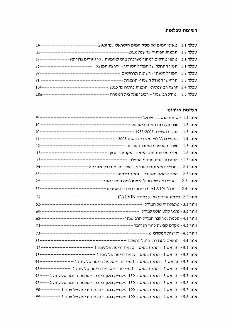
רשימת טבלאות
14)2020עד (מאזני המי! של משק המי! הישראלי : 1.1טבלה
152010תוכנית הפיתוח עד שנת : 1.2טבלה
39) או אזורי! גדולי! ( לאומיות לי! לניהול מערכות מי!מיפוי מוד : 2.1טבלה
86 'המוצאהרצת ' המודל השניתי תנאי התחלה של : 5.1טבלה
87 רשימת תרחישי! המודל השנתי : 5.2טבלה
91 תוצאות תרחישי המודל השנתי : 5.3טבלה
104 2015עד תוכנית פיתוח הרצה רב שנתית: 5.4טבלה
106 רכיבי פונקצית המטרה–מודל רב שנתי : 5.5 טבלה
רשימת איורי�
9ישראל שונות הגש! ב 1.1איור
10 בישראלמקורות המי! מפת – 1.2איור
10 20021932עשרה סדרת ה– 1.3איור
11 2003 ביקוש כולל לפי מיגזרי! בשנת – 1.4איור
12 הארצית אספקת המי! מערכת– 1.5איור
13 באקוויפר החו. וניטראטי! מיפוי מליחות– 1.6 איור
15 פריסת מתקני התפלהפיתוח ו 1.7 איור
24תו אזורי מי! בי�העברות –' מחולל המאזני! הארצי ' – 2.1איור
25 תאור סכמתי–' המודל האגרגאטיבי '– 2.2איור
29 טופולוגיה של מודל הסימולציה התלת אגני– 2.3איור
32זרימות מי! בי� אזורית CALVIN מודל – 2.4איור
32 CALVIN סכמת זרימת מידע במודל 2.5איור
52 טופולוגיה של המודל 3.1איור
64 נתוני קלט ופלט למודל 3.2איור
65 סכמת זמ� עבר המודל הרב שנתי 4.1איור
73מקד! קביעת כיוו� הזרימה 4.2איור
73 k רגישות המקד! 4.3איור
82 היטל ההפקה ת הגדרתרשי! ל – 4.4איור
92 1של עונה זרימה כמת ס –הרצת בסיס : 1 תרחיש 5.1איור
93 2 של עונה זרימה זכמת –הרצת בסיס : 1 תרחיש 5.2איור
94 1 של עונה זרימה סכמת �"ירת' מ1+ הרצת בסיס : 2תרחיש 5.3איור
95 2 של עונה זרימה סכמת � "ירת' מ1+ הרצת בסיס : 2 תרחיש 5.4איור
96 1 של עונה זרימה סכמת ק באג� כינרת"למ מ 150+ הרצת בסיס : 3 תרחיש 5.5איור
97 2של עונה זרימה סכמת ק באג� כינרת " מלמ150+ הרצת בסיס : 3 תרחיש 5.6איור
98 1 של עונה זרימה סכמת ק בנגב " מלמ100+ הרצת בסיס : 4 תרחיש 5.7איור
99 2 של עונה זרימה סכמת ק בנגב " מלמ100+ הרצת בסיס : 4 תרחיש 5.8איור

עמוד ) 2המש� (תוכ� הענייני�
79 שליליי! משתני! לא 4.4.5
79 פונקצית מטרה4.5
81 הגדרת עלות הולכה4.5.1
81 היטל הפקה4.5.2
83 עלות התפלה4.5.3
� דוגמאות לתוצאות הרצות וניתוח� : 5פרק ����������������������������������������84
84 הקדמה5.1
84בודדת שנה ת המודל למש/ תוצאות עבור הרצ5.2
84 הרצת מוצא5.2.1
87 תאור תרחישי!5.2.2
87 ניתוח תוצאות5.2.3
104 הרצת המודל הרב שנתי5.3
104 תאור התוצאות5.3.1
108ה השנתית והרב שנתית סיכו! ההרצ 5.4
�מסקנות ודיו� : 6פרק ������������������������������������������������� ������110
110כלליות מתהלי/ המידול מסקנות 6.1
111 מסקנות אסטרטגיות6.2
112 יישומי! אפשריי! בתכנו� ארצי6.3
�נוספי�אפשריי� כיווני מחקר : 7פרק ������������������������������������������113
115 מקורות

עמוד ) המש� (תוכ� הענייני�
56 הכתבת מצב המערכת בנקודות זמ� נבחרות 3.5.4.1
56 תכנו�האופק הזמ� ויחידת ייצוג 3.5.4.2
57 תנאי אי וודאות שיקולי יישו! 3.5.4.3
57 אמינות אספקה3.5.4.4
58 כיול 3.5.4.5
58 נתוני קלט מבנה המודל ו 3.6
59 נתוני היצע3.6.1
59 נתוני העשרה3.6.1.1
59 נתוני מקורות מי!3.6.1.2
60 נתוני ביקוש3.6.2
60 נתוני מערכת ההולכה3.6.3
61קורות נתוני מדיניות ניהול המ 3.6.4
61 נתוני תוכנית הפיתוח3.6.5
61 נתוני התחלה3.6.6
62וני פלט נת3.7
63 והשימוש בתוכנה אופטימיזציהה שיטת 3.8
�ניסוח מתמטי של המודל: 4פרק ������������������������������������������������65
65 הקדמה4.1
65 מימדי המודל4.2
66 משתני החלטה4.3
69 אילוצי!4.4
69 אילוצי! הידרולוגי!4.4.1
73 אילוצי! על מיפלסי המי!4.4.1.1
74 מליחות המי! אילוצי! על 4.4.1.2
74 גלישות באג! כינרת4.4.1.3
74 ביקוש4.4.2
74 ביקוש מינימאלי באזורי ביקוש4.4.2.1
75 ביקושהאזורי מסופקי! למי! ה איכות מיניאלית ב4.4.2.2
75 מערכת ההולכה4.4.3
75 כושר הולכה4.4.3.1
76 משוואות רציפות4.4.3.2
76 משוואות שימור מסה4.4.3.3
77 כושר התפלה4.4.3.4
77 איכות מי! מותפלי!4.4.3.5
78 משתני מצב4.4.4

עמוד יני�יענהתוכ�
רשימת טבלאות
רשימת איורי�
1 תקציר
4 רשימת סמלי�
6 קיצורי�רשימת
�מבוא: 1פרק ���������������������������������������������������������������� 7
7 הקדמה 1.1
8 משק המי! הישראלי 1.2
16מבנה העבודה 1.3
�סיווג מודלי� וסקר ספרות: 2פרק �����������������������������������������������17
17 הקדמה2.1
19 הגדרת איכות מי!2.2
19העוסקי! באיכות מי!שת פותרי רו סיווג מודלי! 2.3
20זרימה מכוונת סיווג מודלי! ע! 2.4
20 מודלי! לניהול משאבי מי!ג סיוו2.5
21 איכות והידראוליקה, בהתייחס לזרימה כמותית סיווג מודלי! לניהול ואספקת מי! 2.6
22 סקירת מודלי! לניהול משק המי!2.7
22 תחו! סקירת המודלי!2.7.1
22 משאבי מי! מודלי! לניהול2.7.2
41 קיצורי! – 2.1 טבלה 2.7.3
44 עבודה זותרומה של ה2.8
�מתודולוגיה: 3פרק �����������������������������������������������������������46
46 הקדמה3.1
48 בניהול משאבי מי!מול סימולציה מיזציה אופטי3.2
48 הירארכיה של מודלי!3.3
50 המודלתחו! הניהול של 3.4
50 של המתודולוגיהמרכיבי! עיקריי! 3.5
50 המדיניותעקרונות תאור 3.5.1
50 מדיניות ניהול הביקוש3.5.1.1
52 מדיניות הפיתוח3.5.1.2
53 קורות מדיניות ניהול המ3.5.1.3
54 אגרגציה והפשטה3.5.2
54 אופטימיזציה כנגד סימולציה3.5.3
56 בר קיימאאילוצי מדיניות פיתוח יישו! 3.5.4

הבעת תודה
, מי� וחקלאות, הנדסת סביבהליחידה באורי שמיר ' המחקר נעשה בהנחיית פרופ
.הפקולטה להנדסה אזרחית וסביבתית במסלול להנדסה וניהול משאבי מי�
אני רוצה להודות מקרב לב על . אורי שמיר' זכיתי ללמוד בהנחיתו של פרופ
ל� פגישותינו אשר החלקי במ מנת שהיו והרגעי� המרתקי� החוויה, ההשראה
ניהול משאבי הקשורי� לשוני� לנושאי� , מעבר לנושא מחקר זהגלשו פעמי� רבות
. מי�
) נציבות המי�, של אג� תכנו�לשעברמנהל ה (יוס� דרייזי�' לדרתודה מיוחדת
במהל� לימודי� הלשלב את לי ואיפשר שעודד אותי ללמוד ניהול משאבי מי�
.תיעבוד
.על התמיכה והעידוד) נציבות המי�, מנהל אג� תכנו�(ברצוני להודות למו פרוביזור
.אני מודה לנציבות המי� על ההשתתפות במימו� השתלמותי
ה ת עזרעלאני רוצה להודות למשפחתי על הסבלנות והתמיכה ובמיוחד לאימי
. הראשונית של עבודה זוהבהגה

כמות ואיכות של שנתי משולב לניהול אופטימלי רב מודל המי� הארציתאספקת במערכת
חיבור על מחקר
קבלת התוארלש� מילוי חלקי של הדרישות ל מגיסטר למדעי� בהנדסה וניהול של משאבי מי�
זיידהמיכאל
מכו� טכנולוגי לישראל–הוגש לסנט הטכניו�
2006 פברוארחיפה ו"תשס

לניהול אופטימלי רב שנתי משולב של מודל כמות ואיכות במערכת אספקת המי� הארצית
מיכאל זיידה