a micro PLUMED Tutorial for FHI-aims users

PLUMED:portable plugin for free-energy calculationswith molecular dynamics

FHI-aims Developers’ and Users’ Meeting

Organized by Fritz Haber Institute,CECAM-mm1p, and CECAM-SCM

Free University Berlin, Berlin, GermanyAugust 28 - August 31, 2012

This document and the relative computer exercises have beenwritten by Davide Branduardi and Luca Ghiringhelli and isbased on a previous tutorial held in CECAM, Lausanne in2010 whose authors are:

Massimiliano BonomiDavide BranduardiGiovanni BussiFrancesco GervasioAlessandro LaioFabio Pietrucci

Tutorial website:http://sites.google.com/site/plumedtutorial2010/

PLUMED website:http://www.plumed-code.org

PLUMED users Google group:plumed-users@googlegroups.com

PLUMED reference article:M. Bonomi, D. Branduardi, G. Bussi, C. Camilloni, D. Provasi, P. Rai-teri, D. Donadio, F. Marinelli, F. Pietrucci, R.A. Broglia and M. Par-rinello, , Comp. Phys. Comm. 2009 vol. 180 (10) pp. 1961-1972.

1

Contents

1 What PLUMED is and what it can do 3

2 Basics: how to enable PLUMED in FHI-aims 6

3 A simple bias on the system 11

4 A moving bias on the system 18

5 A metadynamics example 22

6 Other features and conclusions 30

2

Chapter 1

What PLUMED is and what itcan do

PLUMED is a series of open source (L-GPL) routines that are nowinterfaced to a number of molecular dynamics engines (beyond FHI-aims: NAMD, GROMACS, LAMMPS, ACEMD, SANDER, CPMD,G09-ADMP, and more) that enable the code to perform a number ofenhanced sampling calculations. Its core consists in a routine thattakes the position of the atoms at each timestep and introduces forcesaccording to the specific configuration of the system: this is the coreof many enhanced sampling calculations. Since this is a very tiny linkto the MD code, this can be done in a rather general way and that ison of the main reasons why many MD codes incorporates it.

The usefulness of these enhanced sampling calculations is that theyallow for calculating free-energy differences associated to conforma-tional transitions, chemical reaction and phase transitions.

In general, the free energy of a system in a specific point can bedefined as

F (s) = −1

βlogP (s) (1.1)

where F is the Helmoltz’s free energy, s is a descriptor of the system(a bond distance, angle, or another generic order parameter of somesort), P (s) is the probability that the system is in the state labelled

3

by the descriptor s, β = 1/kBT where kB is the Boltzmann constantand T is the temperature of the system.

Therefore, building an histogram of the conformations is the easiestway one can build a free-energy profile as a function of some parameter.

Unfortunately, very often it happens that the exploration via MDis all but exhaustive. In fact the system may stay trapped in someminimum inasmuch the kinetic energy provided from the thermostat(which is 0.5kBT = 0.3 kcal/mol per degree of freedom at 300 K) veryoften does not allow for the the overcoming of barriers within the usualtime span of a MD simulations (typically tens to hundreds of ps forab initio MD, up to several µs for classical-force-field-based MD). Inthis case we say that the system is in a ”metastable state” which isexemplified in the Fig. 1

In order to illustrate this, let us consider a typical barrier for achemical reaction: ∆U ‡ ' 8 kcal/mol. One can estimate the rate of areaction by using the Arrhenius equation that reads

ν(T ) = ν0 exp−∆U‡

kBT . (1.2)

By considering ν0 for a typical covalent bond, ν0 = 5 109s−1, as an up-per bound, one easily get a rate of 7 103 events per second. Therefore,each single event can well take up to a millisecond and the observationof one single event is (very) fortuitous in the typical timescales of aDFT-based MD. Moreover, since the estimate of the probability re-quires converged statistics, the converged free-energy calculation canrequire even much more time.

What PLUMED can do is to physically displace the system fromwhere it is so that you can measure the slope of the free-energy land-scape in various ways and then reconstruct the free energy or simplymake some event happen. In the next we’ll show some basic function-alities.

4

Figure 1.1: Sketch of the typical case where the dynamics is locked in a metastablestate. Upper panel: the real free energy landscape is represented for a model land-scape. Since the kinetic energy is low compared to the barrier, the crossing is highlyunlikely and the system stays trapped. The observed probability is reported in themiddle panel and in the lower panel is the computed free energy from the histogram.This is clearly different from the actual one which is reported in the upper panel.

5

Chapter 2

Basics: how to enable PLUMEDin FHI-aims

Enabling PLUMED from FHI-aims requires a separate compilation.A separate

Makefile.meta

is provided (see FHI-aims manual).The actual use of the plugin is switched on by this single line in

control.in:

plumed .true.

With plumed .false. (default) or nothing, the code would behaveexactly as compiled without this plugin. It is implied that some MDscheme must be used in control.in, in order to see PLUMED acting.What PLUMED does, in facts, is to modify the molecular dynamicsforces according to the selected scheme.All the specific controls of the free-energy calculation are contained inthe file plumed.dat (which must be in the working directory, togetherwith control.in and geometry.in, if plumed .true. is set).

As a simple example, let’s consider a methyl-chloride molecule anda chlorine ion. This is a well studied system and computationallyconvenient. Additionally, the chlorine anion is able to displace thesecond chlorine and give a SN2 (bimolecular nucleophilic substitution)

6

Figure 2.1: A sketch of SN2 reaction

type of reaction represented in Fig 2.1. This is a well studied system(see [1]) and yet computationally convenient.

Concerning FHI-aims setup, all the results reported below are per-formed with a ”first tier” basis set and an outer grid of 302. Runs ofthis size may take almost two hours on 4 proc machine for 5 ps (typicalrun time in these calculations). In order to fit into a tutorial time,pw-lda density functional and an outer grid of 194 could be used.Here we report a minimal example of plumed.dat that just calculatesa couple of distances between one atom and (the geometric center of)a group of atoms along the simulation:

#

# Note: distances are reported in bohr

#

DISTANCE LIST 1 <g1>

g1->

3 4 5 6

g1<-

DISTANCE LIST 2 <g1>

PRINT W_STRIDE 2

ENDMETA

The first line tells PLUMED that a distance should be calculatedbetween the bound chlorine, which is atom number 1 (the first atomin FHI-aims geometry.in file) and the geometric center of a group

7

of three atom represented by the symbol <g1> that correspond to themethyl group. The notation

g1->

3 4 5 6

g1<-

starts the group, puts the number of the atoms included in it, andcloses the group. The other line DISTANCE LIST 2 <g1> asks forthe calculation of the distance between the unbound chlorine and themethyl group. The line

PRINT W_STRIDE 2

determines that the distance (and other relevant informations) will beprinted later every 2 timesteps in the COLVAR file. Every time that yourestart a simulation, the old COLVAR file is backed up in COLVAR.old

and a new COLVAR file is written. Beware that if you do this two timesthe first COLVAR file will be lost.

PLUMED produces also a PLUMED.OUT file which is very importantfor understanding whether PLUMED is really doing what you asked itto do. We really warmly recommend everyone to give a read to it. Youcan find there also useful citations for specific methods implemented.This file is never backed up and is overwritten every time.

Please note that all the settings and examples reported for thismolecule are meant only to allow you to do some exercise within thetime of the tutorial and are NOT, BY ANY MEANS, similar to agood production setup which is much more computational intensive.Therefore, for the same reasons, we do not enter in the details of thesimulations but for one single exception: the calculation is a moleculardynamics. In our case the input contains a section that looks like:

MD_run 5.0 NVT_parrinello 300 0.1

MD_time_step 0.001

MD_clean_rotations .true.

MD_restart .false.

8

output_level MD_light

MD_MB_init 300

MD_RNG_seed 12345

plumed .true.

which denotes a molecular dynamics setup where one specifies theensemble NVT parrinello 300 0.1 (a stochastic thermostat [2] at300K with a coupling parameter τ of value 0.1 ps), with the initialtemperature set to 300 K (MD MB init 300) and a timestep of 1 fs(MD time step 0.001) which is an upper limit for hydrogen contain-ing molecules (we would recommend 0.25 fs for production). Addition-ally the statement plumed .true. denotes the activation of plumed,therefore a plumed.dat file should be present in the same directorywhere geometry.in and control.in are.

When sending the calculation, one obtains a PLUMED.OUT file inwhich it is reported, among the other things:

::::::::::::::::: READING PLUMED INPUT :::::::::::::::::

|- GROUP FOUND: g1

|- GROUP MEMBERS: 3 4 5 6

1-DISTANCE: (1st SET: 1 ATOMS), (2nd SET: 4 ATOMS); PBC ON

|- DISCARDING DISTANCE COMPONENTS (XYZ): 000

|- 1st SET MEMBERS: 1

|- 2nd SET MEMBERS: 3 4 5 6

2-DISTANCE: (1st SET: 1 ATOMS), (2nd SET: 4 ATOMS); PBC ON

|- DISCARDING DISTANCE COMPONENTS (XYZ): 000

|- 1st SET MEMBERS: 2

|- 2nd SET MEMBERS: 3 4 5 6

|-PRINTING ON COLVAR FILE EVERY 2 STEPS

|-INITIAL TIME OFFSET IS 0.000000 TIME UNITS

9

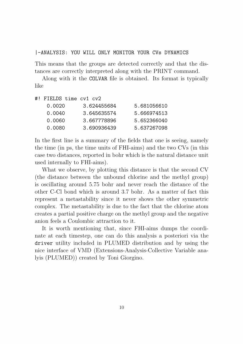
|-ANALYSIS: YOU WILL ONLY MONITOR YOUR CVs DYNAMICS

This means that the groups are detected correctly and that the dis-tances are correctly interpreted along with the PRINT command.

Along with it the COLVAR file is obtained. Its format is typicallylike

#! FIELDS time cv1 cv2

0.0020 3.624455684 5.681056610

0.0040 3.645635574 5.666974513

0.0060 3.667778896 5.652366040

0.0080 3.690936439 5.637267098

In the first line is a summary of the fields that one is seeing, namelythe time (in ps, the time units of FHI-aims) and the two CVs (in thiscase two distances, reported in bohr which is the natural distance unitused internally to FHI-aims).

What we observe, by plotting this distance is that the second CV(the distance between the unbound chlorine and the methyl group)is oscillating around 5.75 bohr and never reach the distance of theother C-Cl bond which is around 3.7 bohr. As a matter of fact thisrepresent a metastability since it never shows the other symmetriccomplex. The metastability is due to the fact that the chlorine atomcreates a partial positive charge on the methyl group and the negativeanion feels a Coulombic attraction to it.

It is worth mentioning that, since FHI-aims dumps the coordi-nate at each timestep, one can do this analysis a posteriori via thedriver utility included in PLUMED distribution and by using thenice interface of VMD (Extensions-Analysis-Collective Variable ana-lyis (PLUMED)) created by Toni Giorgino.

10

Chapter 3

A simple bias on the system

Now let’s try to apply a simple harmonic bias, often called “harmonicpotential”, that stretches the bond and thus “encourages” the transi-tion. This is the first example that shows how PLUMED biases thesimulation.

First, in addition to the previous descriptor, we add another one,namely the difference between the two distances. This is a rather wellknown and used descriptor whenever some bond breaking/bond form-ing reaction is involved since, by moving from one value to its negative(in the case of such symmetric reaction), it allows to simultaneouslybreaking one bond while forming another one.

The plumed.dat file therefore will look like:

#

# monitor the two components

#

g1->

3 4 5 6

g1<-

DISTANCE LIST 1 <g1>

DISTANCE LIST 2 <g1>

PRINT W_STRIDE 1

# the distance between C-Cl’ and C-Cl

DISTANCE LIST 1 <g1> DIFFDIST 2 <g1>

UMBRELLA CV 3 AT 0.0 KAPPA 0.01

11

ENDMETA

Note that here we have additionally put the directive:UMBRELLA CV 1 AT 0.0 KAPPA 0.01

This enables the addition of the harmonic potential that has the form:

Ubias(x) =k

2(CV (x)− CV0)2 (3.1)

in which AT determines the CV0, KAPPA determines the k value. In thiscase the units of k are hartee/bohr2 so that the energy is in hartree.

The output of PLUMED.OUT in this case shows a line like

|-UMBRELLA SAMPLING OF COLVAR 3 AT 0.00: SPRING=0.010 SLOPE=0.00

which denotes the addition of the harmonic bias.The output of COLVAR changes in something like:

#! FIELDS time cv1 cv2 cv3 vwall XX XX RST3 WORK3

0.002 3.604 5.694 -2.090 0.021 RST 3 0.000 0.000

0.004 3.668 5.644 -1.975 0.019 RST 3 0.000 0.000

0.006 3.709 5.607 -1.897 0.018 RST 3 0.000 0.000

0.008 3.768 5.555 -1.787 0.015 RST 3 0.000 0.000

0.010 3.834 5.495 -1.661 0.013 RST 3 0.000 0.000

0.012 3.898 5.434 -1.535 0.011 RST 3 0.000 0.000

in which it appears a new field: vwall. This is the potential energycalculated by the harmonic potential. The other remaining fields onthe right are only relevant with a moving restraint (see below).

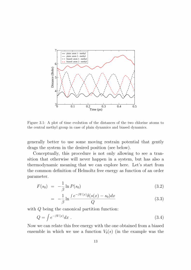
Now, in order to compare with the unbiased results, let’s comparethe two bond distances in the plain simulation and in the biased one.In Fig. 3.1 it is evident that the umbrella potential is biasing the twodistance toward a set of values whose difference is centered on zerovalue. Since at the beginning the simulation is starting far from thezero value imposed by the umbrella potential, initially the simulationis dominated by this spring and oscillates strongly around the centerof the harmonic potential. Generally this behavior disappeares aftera while, when the system reaches equilibrium. For this reason it is

12

0 0.1 0.2 0.3 0.4 0.5Time (ps)

3

4

5

6

7D

ista

nce

(Boh

r)plain: atom 1 - methylplain: atom 2 - methylbiased: atom 1 - methylbiased: atom 2 - methyl

Figure 3.1: A plot of time evolution of the distances of the two chlorine atoms tothe central methyl group in case of plain dynamics and biased dynamics.

generally better to use some moving restrain potential that gentlydrags the system in the desired position (see below).

Conceptually, this procedure is not only allowing to see a tran-sition that otherwise will never happen in a system, but has also athermodynamic meaning that we can explore here. Let’s start fromthe common definition of Helmoltz free energy as function of an orderparameter.

F (s0) = −1

βlnP (s0) (3.2)

= −1

βln

∫e−βV (x)δ(s(x)− s0)dx

Q(3.3)

with Q being the canonical partition function:

Q =∫e−βV (x)dx . (3.4)

Now we can relate this free energy with the one obtained from a biasedensemble in which we use a function Vb(s) (in the example was the

13

harmonic function). This would read

Fb(s0) = −1

βlnPb(s0) (3.5)

= −1

βln

∫e−β(V (x)+Vb(s(x)))δ(s(x)− s0)dx

Qb(3.6)

with

Qb =∫e−β(V (x)+Vb(s(x))dx (3.7)

Since all the points selected by the delta function δ(s(x)− s0) presentthe same value of Vb(s(x)), the exponential related to the bias can bepulled out from the integral to give:

Fb(s0) = −1

βln e−βVb(s0)

∫e−βV (x)δ(s(x)− s0)dx

Qb(3.8)

= Vb(s0)−1

βln

∫e−βV (x)δ(s(x)− s0)dx

Qb(3.9)

= Vb(s0)−1

βlnP (s)

Q

Qb(3.10)

= Vb(s0)−1

βlnP (s) +

1

βlnQ

Qb(3.11)

= Vb(s0)−1

βlnP (s) + C (3.12)

Fb(s0) = Vb(s0) + F (s0) + C (3.13)

from which one has:

F (s0) = Fb(s0)− Vb(s0) + C (3.14)

that means that, from a biased simulation, one can retrieve the cor-rect free energy just by knowing the bias and the histogram in thebiased ensemble. So, if one can find a function that compensates thefree-energy landscape, then the system is free to travel in the spaceof CVs and the histogram can be acquired with accuracy since all themetastabilities are removed. This is crucial for many enhanced sam-pling methods, e.g., Metadynamics (MetaD) [3] that relies exactly onan iterative procedure aimed to produce the compensating potential.

14

-2 -1.5 -1 -0.5 0 0.5 1 1.5 2DIfference of distances (Bohr)

0

0.01

0.02

0.03

0.04

0.05

0.06

0.07

Prob

abili

ty

Figure 3.2: A sketch of the distribution from the umbrella potential for the SN2reaction.

Let’s try this approach on this case. Please consider that, in orderto obtain a good-quality estimate of the free energy, one should havea long trajectory and check the convergence, the easiest way being thecomparison of histograms from the first half of the trajectory and thesecond half of the trajectory. First we retrieve the probability fromthe trajectory. This can be done with the awk script provided.

grep -v FIELDS COLVAR >f1

awk ’{print $1,$4}’ f1 |./distribution.awk >dist

then the free energy can be calculated with one liner in gnuplot

p "dist" u 1:(-(0.597)*log($2)-0.5*0.01*627.51*($1*$1)) w lp

that aim to plot the probability of the biased ensemble -(0.597)*log($2)where 0.597 is kBT in kcal/mol at 300K and -0.5*0.01*627.51*($1*$1)

15

-2 -1.5 -1 -0.5 0 0.5 1 1.5 2DIfference of distances (Bohr)

-10-8-6-4-202468

101214

Free

ene

rgy

(kca

l/mol

)

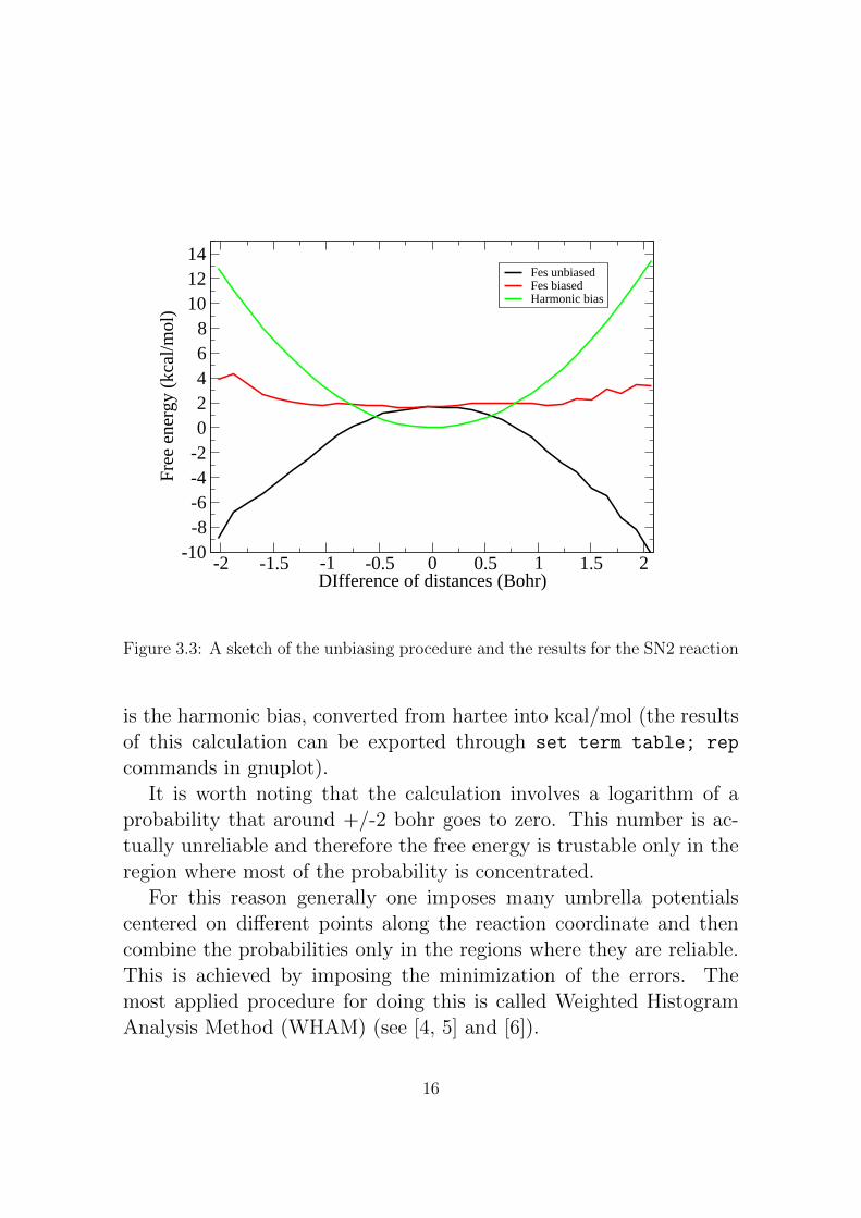
Fes unbiasedFes biasedHarmonic bias

Figure 3.3: A sketch of the unbiasing procedure and the results for the SN2 reaction

is the harmonic bias, converted from hartee into kcal/mol (the resultsof this calculation can be exported through set term table; rep

commands in gnuplot).It is worth noting that the calculation involves a logarithm of a

probability that around +/-2 bohr goes to zero. This number is ac-tually unreliable and therefore the free energy is trustable only in theregion where most of the probability is concentrated.

For this reason generally one imposes many umbrella potentialscentered on different points along the reaction coordinate and thencombine the probabilities only in the regions where they are reliable.This is achieved by imposing the minimization of the errors. Themost applied procedure for doing this is called Weighted HistogramAnalysis Method (WHAM) (see [4, 5] and [6]).

16

Another necessary word is to be spent on the plausibility of results:a plot like the one shown in Fig. 3.2 is clearly suspicious since thereaction should be symmetric while the distribution has some spikes.This is generally a sign of bad convergence. This is of course inevitablein the short running time of a tutorial but should be carefully checkedin production runs and its origin should be understood. Very oftenit is the character of the descriptor itself that can produce variousaberrations since it may compress the phase space in anisotropic way.This is not a problem as far as it is understood as an issue differentfrom the convergence of the calculations.

17

Chapter 4

A moving bias on the system

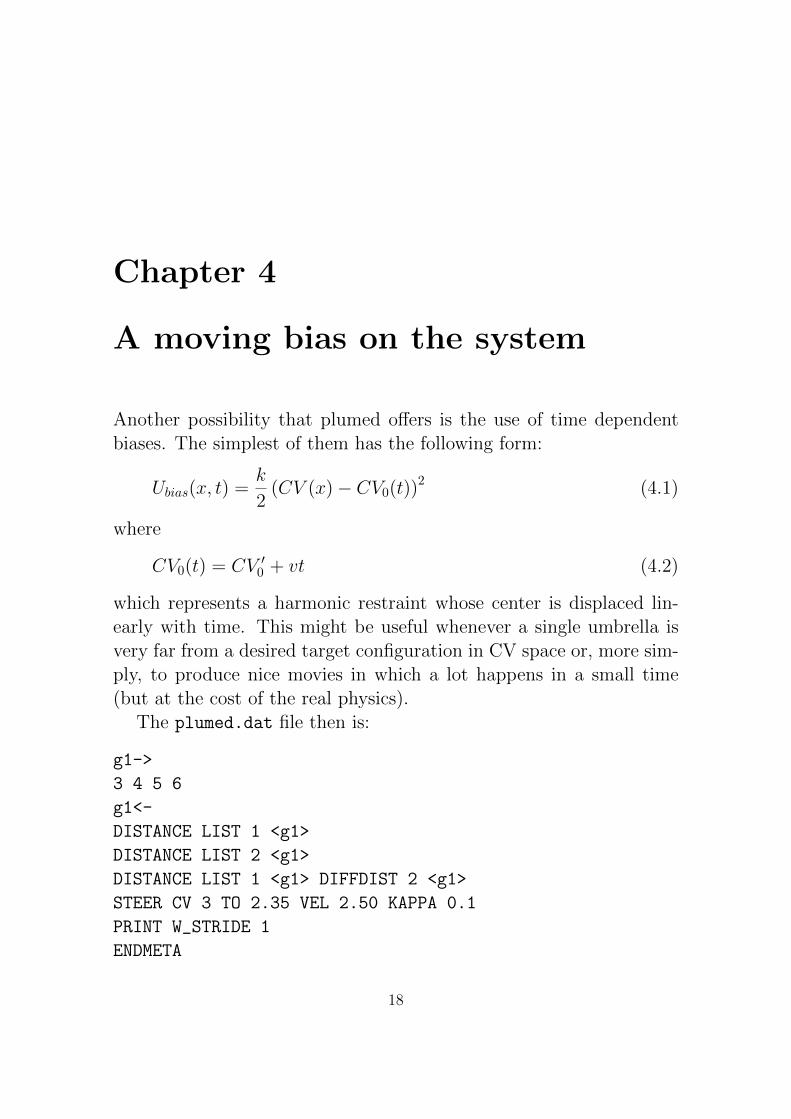
Another possibility that plumed offers is the use of time dependentbiases. The simplest of them has the following form:

Ubias(x, t) =k

2(CV (x)− CV0(t))2 (4.1)

where

CV0(t) = CV ′0 + vt (4.2)

which represents a harmonic restraint whose center is displaced lin-early with time. This might be useful whenever a single umbrella isvery far from a desired target configuration in CV space or, more sim-ply, to produce nice movies in which a lot happens in a small time(but at the cost of the real physics).

The plumed.dat file then is:

g1->

3 4 5 6

g1<-

DISTANCE LIST 1 <g1>

DISTANCE LIST 2 <g1>

DISTANCE LIST 1 <g1> DIFFDIST 2 <g1>

STEER CV 3 TO 2.35 VEL 2.50 KAPPA 0.1

PRINT W_STRIDE 1

ENDMETA

18

where the added line with the directive STEER is gently dragging thesystem to the value of 2.35 bohr with a velocity of 2.5 bohr each 1000steps. The spring constant is set 0.1 hartree/bohr2 and the initial cen-ter CV ′0 is taken as the value of the descriptor at the initial step. ina simulation where there is a time dependent restraint very often, es-pecially for small systems, a more aggressive thermostatting (reducedperiod) is needed to dissipate the thermal energy externally added bythe moving potential. This is true also for metadynamics.

It is important to bear in mind that such ”steered MD” simula-tions may have very little physical meaning and are here reportedjust to let the reader be familiar with PLUMED and its capabili-ties. The reason behind their limited usefulness is that in most ofthe cases these are ”out-of-equilibrium” simulations and they are notrepresentative of equilibrium ensemble that is generally of interest forsimulations. However, Jarzynski [7] inequality provides a connectionbetween out-of-equilibrium trajectories and equilibrium free energydifferences. This inequality consists in:

∆F = −β−1 ln < exp(−βW ) > (4.3)

where the average is calculated over the work obtained from a numberof out-of-equilibrium trajectories. The value of W can be obtained via

W =∫ ts

0dt∂Hb(x, t)

∂t(4.4)

where Hb is a modified hamiltonian which contains an additional term,namely:

Hb(x, t) = H(x) + Ubias(x, t) (4.5)

From which it comes naturally that the derivative is simply:

∂Hb(x, t)

∂t= −vk(CV (x)− CV ′0 − vt) (4.6)

= −vk(CV (x)− λ(t)) (4.7)

and therefore the integral W can be obtained simply by quadraturesumming up all the deviation respect to the position of the mobile

19

center of the harmonic restraint. In the limit of lots of pulling thereforemeaningful free-energy differences can be retrieved.

The COLVAR output reads

#! FIELDS time cv1 cv2 cv3 XX XX RST3 WORK3

0.0020 3.604 5.694 -2.090 RST 3 -2.090 0.000000000

0.0040 3.642 5.669 -2.026 RST 3 -2.088 -0.000011999

0.0060 3.655 5.662 -2.006 RST 3 -2.085 -0.000029506

0.0080 3.669 5.658 -1.988 RST 3 -2.083 -0.000051119

0.0100 3.680 5.658 -1.978 RST 3 -2.080 -0.000075653

0.0120 3.685 5.665 -1.979 RST 3 -2.078 -0.000100674

where in the RST3 column it is reported the center of the movingharmonic potential and in the WORK3 the accumulated work up tothat time (in hartree units).

It is rather important to understand that a calculation of such kindcan be very challenging since the exponential average in Eq. 4.3 tendsto give enormous weight to the trajectories that have less work. Ad-ditionally, slow steering speed and tight spring constant in which thedescriptor follows closely the center of the moving harmonic poten-tial generally deliver better results but in general, if the descriptoris wrong or the landscape is dominated by entropy and is degenerate(presents multiple pathways), generally it is not advisable to use thistechnique.

Additionally it is worth mentioning that forward and backwardpulling can be combined via the Crooks’ theorem [8].

The resulting work profile 4.2 is rather plausible if compared with[1]. The reason for this is that the system presents very few orthogonaldegrees of freedom and is highly symmetrical, therefore the pathwaysare not degenerate and the reaction coordinate is well oriented respectto the real reaction coordinate. This is a rather unique case since inmany other systems the value of work can be as large as 10-fold theexpected free energy.

20

0 0.5 1 1.5 2 2.5 3 3.5Time (ps)

-3

-2

-1

0

1

2

3D

iffer

ence

of d

ista

nces

(Boh

r)

Instantaneous valueCenter of the harmonic potential

Figure 4.1: The instantaneous value of the descriptor follows closely the red line ofthe center of the harmonic potential.

-2 -1.5 -1 -0.5 0 0.5 1 1.5 2Difference of distances (Bohr)

0

2

4

6

8

Wor

k (k

cal/m

ol)

Figure 4.2: The value of work along the difference of distances.

21

Chapter 5

A metadynamics example

Metadynamics adds an adaptive potential to the simulation that growswith simulation time. Intuitively its functioning relies on Eq. 3.14and, in order to find the best possible approximation to the perfectlycompensating bias it adopts a history dependent potential. This biaspotential acts on a restricted number of degrees of freedom of thesystem s(x) = (s1(x), ..., sd(x)) often referred to as collective variablesor CVs. The metadynamics potential V (s, t) varies with time t and isconstructed as a sum of Gaussian functions, or hills, deposited duringthe simulation:

V (s, t) =∫ t

0dt′ω exp

− d∑i=1

(si(x)− Si(x(t′))2

2σ2i

, (5.1)

where σi is the Gaussian width corresponding to the i-th CV and ωthe rate at which the bias grows. In the practice, Gaussians of heightequal to W are deposited every τ MD steps, so that ω = W/τ .

The function of these Gaussian potentials is to discourage the sys-tem to revisit the previously visited points in CV space and reach thepoint in which all the points in CV space are equally sampled in timethat delivers a flat histogram which has no contribution on the freeenergy. Under this assumption the Helmoltz free energy results to bethe negative of the deposited bias.

In order to perform a metadynamics simulation we have to:

• Choose wisely the set of CVs to address the problem. This isa long story. To cut it short, CVs a) should clearly distinguish

22

between the initial state, the final state and the intermediates, b)should describe all the slow events that are relevant to the processof interest, c) their number should not be too large, otherwise itwill take a very long time to fill the free energy surface.

• Choose the Gaussian height W and the deposition stride τ . Thesetwo variables determine the rate of energy added to your simula-tion. If this is too large, the free-energy surface will be explored ata fast pace, but the reconstructed profile will be affected by largeerrors. If the rate is small, the reconstruction will be accurate,but it will take a longer time. The error on the reconstructedFES depends on the ratio W/τ , not on the two parameters alone[9].

• Choose the Gaussian width σi. This parameter determines theresolution of the reconstructed FES. The sum of Gaussians re-produces efficiently (i.e. in a finite simulation time) features ofthe FES on a scale larger than σi. A practical rule is to choosethe width as a fraction (half or one third) of the CV fluctuationsin an unbiased simulation. This is not a golden rule, since thevalue of the fluctuations is not universal but usually depends onthe position in the CV space (see Fig. 5.1 for the calculationof the fluctuation on the CVs used for tracking the unbiased dy-namics). In particular, although intuitively a larger σ could bringto a faster filling, very often, when the choice is not clear as in5.1 it is much better to adopt the smaller one since it guaranteesa better resolution and ability to fill up both narrow and largewells.

To activate a metadynamics calculation in PLUMED you have to usethe directive HILLS. The deposition stride τ is specified in unit of timesteps by the keyword W STRIDE, the height W by HEIGHT in internalunits of energy of the MD code used. The Gaussian width σi must bespecified on the line of each CVs with the keyword SIGMA.

23

3.5 4 4.5 5 5.5 6 6.5 7Distance Methyl-Chloride (Bohr)

0

0.01

0.02

0.03

0.04

0.05

0.06

0.07

Prob

abili

ty

dist1: distributiondist2: distributiondist1: gaussian fitdist2: gaussian fit

Figure 5.1: The fluctuation calculated during the unbiased dynamics for the twomethyl-chloride distances. A gaussian fit is overlapped with the distribution calcu-lated. The σ=0.11 bohr for the black profile and σ=0.440 bohr for the red profile.

24

Generally metadynamics is to be preferred for multidimensionalproblems that require no more than 3/4 CVs. The reason is that inmetadynamics one does not need to explore all the space in CV to havean estimate of the free-energy landscape in a region of interest sincemetadynamics start exploring and filling with potential the regions atlow free energy, which are the most interesting. In other methods, likeWHAM combined with e.g. umbrella sampling, one has to define apriori the grid and the systematic exploration becomes cumbersomein a high-dimensional space.

For the usual case of the SN2 reaction one could think that, insteadof exploring the difference of distances, one could be interested inexploring independently the two methyl-chloride distances (so thatwe show how to set up a multidimensional calculation). Nevertheless,we expect that we are not really interested in unbound states wherethe methyl-Cl distance is above 6.5 Bohr. This require to introducean artificial soft wall to prevent the system from visiting nonreactiveregions which might be trivially low in energy.

A possible input therefore reads:

DISTANCE LIST 1 <g1> SIGMA 0.11

g1->

3 4 5 6

g1<-

DISTANCE LIST 2 <g1> SIGMA 0.11

UWALL CV 1 LIMIT 7. KAPPA 0.5

UWALL CV 2 LIMIT 7. KAPPA 0.5

HILLS HEIGHT 0.00047 W_STRIDE 50

PRINT W_STRIDE 2

ENDMETA

which present a SIGMA value for each of the CVs on which the meta-dynamics is active (it could be a subset of all the CVs) and a specificline starting with HILLS that specify the height and the depositiontime. Additionally we included the confining potential, denoted byUWALL (upper wall) which impose a quartic wall in order to prevent

25

the system to escape from the reactive region.The typical COLVAR files that one obtains is similar to this:

#! FIELDS time cv1 cv2 vbias vwall

0.8240 3.723740474 6.868711550 0.000029924 0.000000000

0.8280 3.691187802 6.931429351 0.000013739 0.000000000

0.8320 3.639273674 6.998560142 0.000004823 0.000000000

0.8360 3.558399168 7.083118628 0.000000000 0.000023865

0.8400 3.478637841 7.159044915 0.000000000 0.000319926

0.8440 3.424739803 7.208958444 0.000000000 0.000953256

0.8480 3.428390769 7.207133491 0.000000000 0.000920389

0.8520 3.493585587 7.155388196 0.000000000 0.000291502

0.8560 3.601809461 7.072873461 0.000000000 0.000014101

0.8600 3.707646538 6.990032405 0.000002236 0.000000000

0.8640 3.779941165 6.922057261 0.000001894 0.000000000

0.8680 3.815026536 6.863783677 0.000004640 0.000000000

0.8840 3.708208013 6.668182930 0.000348923 0.000000000

in which two additional fields are present vbias which is the potentialenergy due to the hills potentials of metadynamics and vwall whichis the potential exerted by the quartic wall (in fact is acting only forvalues of the second CV larger than 7).

In addition to this, PLUMED produces a HILLS. For two-dimensionalGaussian potentials each line consists of time, the position of the cen-ters in the two dimension, the width of the Gaussian potential in thetwo dimensions (in bohr since distances are used as CVs), the height(in hartree) and a multiplicative factor that is only useful when well-temperered metadynamics[14] is enabled.

0.100 3.797 5.972 0.110 0.110 0.00047 0.000

0.200 3.731 6.191 0.110 0.110 0.00047 0.000

0.300 3.668 5.823 0.110 0.110 0.00047 0.000

0.400 3.769 5.619 0.110 0.110 0.00047 0.000

26

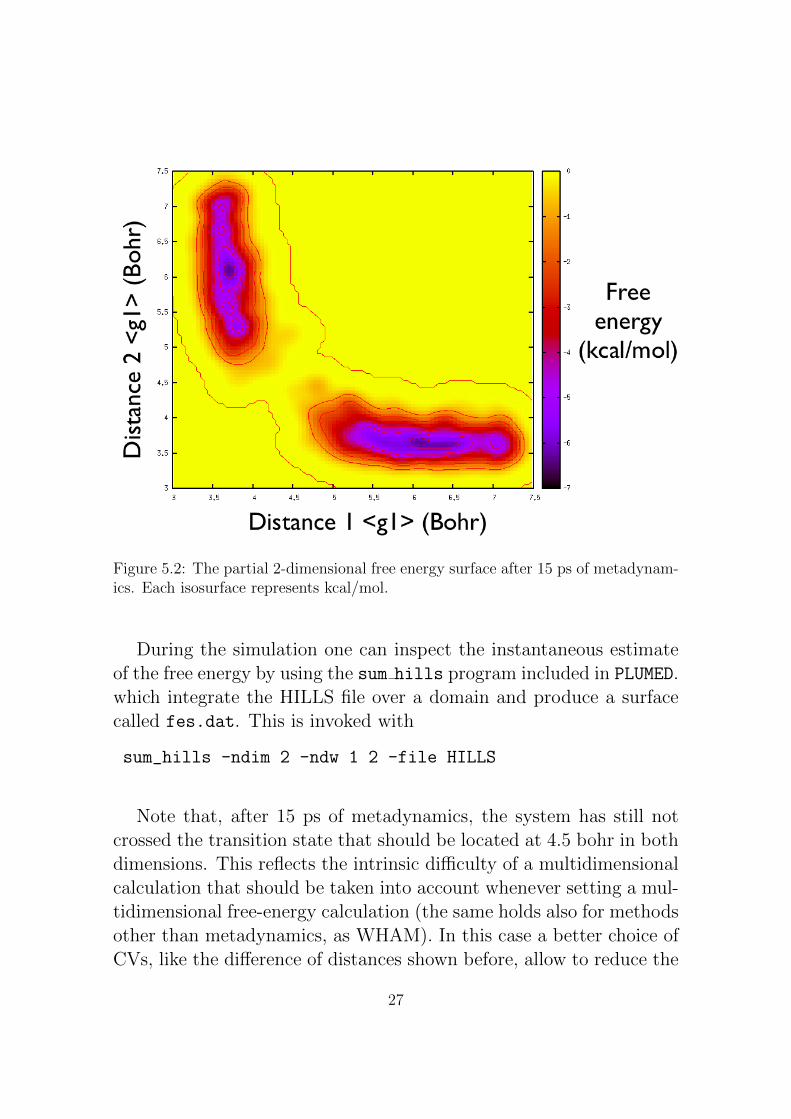
Figure 5.2: The partial 2-dimensional free energy surface after 15 ps of metadynam-ics. Each isosurface represents kcal/mol.

During the simulation one can inspect the instantaneous estimateof the free energy by using the sum hills program included in PLUMED.which integrate the HILLS file over a domain and produce a surfacecalled fes.dat. This is invoked with

sum_hills -ndim 2 -ndw 1 2 -file HILLS

Note that, after 15 ps of metadynamics, the system has still notcrossed the transition state that should be located at 4.5 bohr in bothdimensions. This reflects the intrinsic difficulty of a multidimensionalcalculation that should be taken into account whenever setting a mul-tidimensional free-energy calculation (the same holds also for methodsother than metadynamics, as WHAM). In this case a better choice ofCVs, like the difference of distances shown before, allow to reduce the

27

dimensionality of the problem and allow a faster exploration.Another important fact that should be taken into account when

running a metadynamics run is that it allows for a ”prior”, whichmeans that at the beginning the free-energy landscape is assumed flat(no hills). With the evolution of the bias potential, the estimate of freeenergy landscape is progressively revised and improved. Nevertheless,those regions for which the potential is zero means that they are notsampled by metadynamics and therefore should not be interpreted.For other methods based on the logarithm of probabilities this wouldturn into the negative logarithm of zero which is infinite and thereforecannot be interpreted.

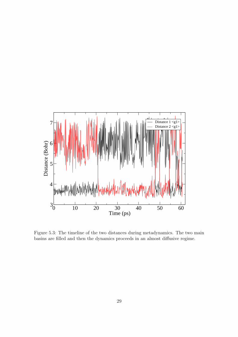
After more than 20 ps of metadynamics the transition state iscrossed and the system spends other more than 20 ps to fill the sec-ond basin. After that point the system spends considerable less timefor each transition and the transition state is repeatedly recrossed.Within this regime the metadynamics can be considered to provide avalid representation of the free energy. Additionally it is worth remem-bering that metadynamics samples the lowest basin first, therefore itscales with a computational effort which is less then a power law ofthe dimensionality used in the metadynamics itself if the landscape isnot too complex.

28

0 10 20 30 40 50 60Time (ps)

3

4

5

6

7

Dis

tanc

e (B

ohr)

Distance 1 <g1>Distance 2 <g1>

Figure 5.3: The timeline of the two distances during metadynamics. The two mainbasins are filled and then the dynamics proceeds in an almost diffusive regime.

29

Chapter 6

Other features and conclusions

This brief summary is intended only to give a first approach to the free-energy calculation problem with PLUMED. We recommend, before em-barking any serious project, to devote time to read the literature andin particular the classic books [10, 11, 12] to acquire a solid backgroundin both simulation techniques and statistical mechanics. PLUMED itselfincludes many more techniques than those outlined here. Among allit is worth citing multiple walkers metadynamics [13], well-temperedmetadynamics [14], d-AFED [15],well-tempered ensemble[16] recon-naissance metadynamics [17] to name a few that are implementedan ready to use in conjuction with FHI-aims (other replica-exchange-based methods will be available soon on a script based method asthe plain replica exchange MD already available for FHI-aims, seemanual). Additionally, flexible steering schedules are available viaSTEERPLAN directives. More than this, PLUMED allows to have plentyof CVs available: from angles to torsion to coordination number up topath collective variables [18]. The investigation of the optimal spacefor projection of the free energy is a very active field indeed.

This is rather central every time one wants to perform a free-energycalculation and should be carefully explored and analyzed. Literaturevery often helps a lot in this respect.

30

Bibliography

[1] S. Yang, P. Fleurat-Lessard, I. Hristov, T. Ziegler, Free en-ergy profiles for the identity s(n)2 reactions cl-+ch3cl andnh3+h3bnh3: A constraint ab initio molecular dynamics study, JPhys Chem A 108 (43) (2004) 9461–9468.

[2] G. Bussi, D. Donadio, M. Parrinello, Canonical sampling throughvelocity rescaling, Journal Of Chemical Physics 126 (1).

[3] A. Laio, M. Parrinello, Escaping free energy minima, Proc. Natl.Acad. Sci. USA 99 (2002) 12562–12566.

[4] S. Kumar, J. M. Rosenberg, D. Bouzida, R. H. Swendsen, P. A.Kollman, Multidimensional free-energy calculations using theweighted histogram analysis method, J. Comput. Chem. 16 (1995)1339–1350.

[5] B. Roux, The calculation of the potential of mean force usingcomputer-simulations, Comput. Phys. Comm. 91 (1995) 275–282.

[6] A. Grossfield, WHAM.http://membrane.urmc.rochester.edu/Software/WHAM/WHAM.html.

[7] C. Jarzynski, Nonequilibrium equality for free energy differences,Phys. Rev. Lett. 78 (1997) 2690–2693.

[8] G. Crooks, Nonequilibrium measurements of free energy differ-ences for microscopically reversible markovian systems, J. Stat.Phys. 90 (5-6) (1998) 1481–1487.

31

[9] A. Laio, A. Fortea-Rodriguez, F.Gervasio, M. Ceccarelli, M. Par-rinello, Assessing the accuracy of metadynamics, J. Phys. Chem.B 109 (2005) 6714–6721.

[10] M. P. Allen, D. J. Tildesley, Computer Simulation of Liquids,Oxford University Press, New York, 1987.

[11] D. Frenkel, B. Smit, Understanding molecular simulation, Aca-demic Press, 1996.

[12] D. Chandler, Introduction to modern statistical mechanics, Ox-ford University Press, 1987.

[13] P. Raiteri, A. Laio, F. Gervasio, C. Micheletti, M. Parrinello, Effi-cient reconstruction of complex free energy landscapes by multiplewalkers metadynamics, J. Phys. Chem. B 110 (2006) 3533–3539.

[14] A. Barducci, G. Bussi, M. Parrinello, Well-tempered metady-namics: A smoothly converging and tunable free-energy method,Phys. Rev. Lett. 100 (2) (2008) 020603.

[15] J. B. Abrams, M. E. Tuckerman, Efficient and direct generationof multidimensional free energy surfaces via adiabatic dynamicswithout coordinate transformations, J. Phys. Chem. B 112 (2008)15742–15757.

[16] M. Bonomi, M. Parrinello, Enhanced sampling in the well-tempered ensemble, Phys. Rev. Lett. 104 (2010) 190601.

[17] G. A. Tribello, J. Cuny, H. Eshet, M. Parrinello, Exploring thefree energy surfaces of clusters using reconnaissance metadynam-ics, J. Chem. Phys 135 (11) (2011) 114109.

[18] D. Branduardi, F. L. Gervasio, M. Parrinello, From A to B in freeenergy space, J. Chem. Phys. 126 (5) (2007) 054103.

32