a methodology for selecting portfolios of projects with ...tavana.us/publications/ijpm-dea.pdf ·...

Available online at www.sciencedirect.com

International Journal of Project Management 30 (2012) 791–803www.elsevier.com/locate/ijproman

A methodology for selecting portfolios of projects with interactionsand under uncertainty

Amir Hossein Ghapanchi a,⁎, Madjid Tavana b, Mohammad Hossein Khakbaz c, Graham Low d

a School of Information and Communication Technology, Griffith University, Gold Coast Campus, Queensland, Australiab Management Information Systems, Lindback Distinguished Chair of Information Systems, La Salle University, Philadelphia, PA 19141, USA

c Institute of Transport and Logistics Studies, Sydney University, Sydney, Australiad Information Systems, School of Information Systems, Technology and Management, The University of New South Wales, Sydney, Australia

Received 15 September 2010; received in revised form 18 January 2012; accepted 24 January 2012

Abstract

Effective project evaluation and selection strategies can directly impact organizational productivity and profitability. Numerous analytical tech-niques ranging from simple weighted scoring to complex mathematical programming approaches have been proposed to solve these problems.However, traditional project selection methods too often fail to consider both the uncertainties in projects and the interaction among projects. Someprior studies have considered the interaction among projects in deterministic environments. Others have dealt with stochastic environments buthave not considered project interdependencies. This study aspires to fill this gap in the project portfolio selection literature. Information system/information technology (IS/IT) projects are used in this study because they are frequently subject to uncertainties due to estimation difficultiesand bounded by interactions due to technological interdependencies. We use Data Envelopment Analysis (DEA) to select the best portfolio ofIS/IT projects while taking both project uncertainties (modeled as fuzzy variables) and project interactions into consideration simultaneously.We also present a numerical example to demonstrate the applicability of the proposed framework and exhibit the efficacy of the procedures.© 2012 Elsevier Ltd. APM and IPMA. All rights reserved.

Keywords: IS/IT project; Portfolio selection; Data envelopment analysis; Fuzzy set theory

1. Introduction

Many organizations have been increasing their investments inInformation Systems/Information Technologies (IS/IT) to meetthe growing demands for efficiency and effectiveness(Gunasekarana et al., 2001). Rivard et al. (2006) argue thatwell-planned IS/IT investments that are carefully selected with re-spect to business mission requirements can have a positive impacton organizational performance. Conversely, IS/IT investmentsthat are poorly planned, can postpone or severely limit organiza-tional performance (Gunasekarana et al., 2001). Farbey et al.(1999) have commented “There is concern that poor evaluationprocedures mean it is difficult to select projects for investment,to control development and to measure business return after

⁎ Corresponding author.E-mail address: [email protected] (A.H. Ghapanchi).

0263-7863/$36.00 © 2012 Elsevier Ltd. APM and IPMA. All rights reserved.doi:10.1016/j.ijproman.2012.01.012

implementation [p. 189]”. Often organizations need to choose be-tween a number of competing IS/IT investments for various rea-sons including limited resources and capacity constraints.

Many theoretical and practical models have been developed tosupport the process of project portfolio selection. Early attemptsfocused on constrained optimization methods were given a set ofcandidate projects; the goal is to select a subset of projects to max-imize some objective function without violating the constraints(Danila, 1989). Some prior studies have considered the interactionamong projects in deterministic environments (i.e. Bardhan et al.,2004; Eilat et al., 2006). Others have dealt with stochastic environ-ments but have not considered project interdependencies (i.e.Chen and Cheng, 2009; Huang et al., 2008; Lin and Hsieh,2004; Tiryaki and Ahlatcioglu, 2005, 2009). As a result, thesemodels have not found widespread use in practice (Eilat et al.,2006). This study aspires to fill this gap in the project portfolio se-lection literature. We use Data Envelopment Analysis (DEA) to

mailto:[email protected]

http://dx.doi.org/10.1016/j.ijproman.2012.01.012




792 A.H. Ghapanchi et al. / International Journal of Project Management 30 (2012) 791–803

select the best portfolio of projects taking both project uncer-tainties (modeled as fuzzy variables) and project interactions intoconsideration simultaneously. Another contribution of this studyis the application of fuzzy DEA (FDEA) for project portfolio se-lection. This approach has not been undertaken previously, andpromises to enrich considerably the decision making technology.

IS/IT projects are Research and Development (R&D) projectswith some distinctive features (Møen, 2005). However, IS/IT pro-jects have certain attributes that differentiate them from the othertypes of R&D projects (Møen, 2005). For example, adoption ofIS/IT initiatives can be more lengthy, expensive and complex(Gunasekarana et al., 2001). IS/IT investments also tend to havea high failure rate that might have potentially devastating impacts(Wu and Ong, 2008). One of the most critical characteristics ofIS/IT investments that differentiates them from the other typesof R&D projects is the high degree of risk and uncertainty associ-ated with them (Bacon, 1992; Gunasekarana et al., 2001; Irani etal., 2002; Wu and Ong, 2008). IS/IT projects involve technologi-cal as well as organizational uncertainties (Wu and Ong, 2008).Technological uncertainty originates from rapid change in suchtechnologies; therefore, investments might become obsoletequickly. Organizational uncertainty ranges from unpredictableuser resistance, the cost of employee burnout, and themaintenanceexpenses (Wu and Ong, 2008). Interdependencies also existamong the projects because they normally support common objec-tives (Eilat et al., 2006), use shared input and often impact eachother's output. The complexity of IS/IT projects as well as their in-terdependencies poses a challenge when applying methods for theprioritization of these investments (Bardhan et al., 2004). That iswhy researchers have criticized conventional methods for evaluat-ing IS/IT investments (e.g. Farbey et al., 1993). This study focuseson IS/IT projects because these projects typically demonstrateboth interdependency and project uncertainty.

This paper is organized as follows. In Section 2 we present abrief literature review on project portfolio selection. We then de-scribe the proposed methodology in Section 3. In Section 4 weillustrate the proposed methodology using a numerical example.In Section 5 we present our concluding remarks and in Section 6we discuss our research limitations and future research directions.

2. Research background

In this section we first review the literature on portfolio se-lection and then describe DEA and FDEA.

2.1. Portfolio selection

Achieving maximal project portfolio value for the resourcesused is often complicated by multiple selection criteria, subjec-tive and imprecise assessments and project interdependencies(Ravanshadnia et al., 2010, 2011). Danila (1989) defines portfo-lio selection as selecting an investment from a list of candidateinvestments in order to maximize some objectives without violat-ing constraints. Cooper et al. (1997) categorize portfolio selectionproblems into two categories: dynamic and static. Bard et al.(1988) suggest that in the dynamic approach, we face projectsthat are in progress (active projects) and those that have not

started yet (candidate projects). Static portfolio selection involvesevaluating portfolios of candidate projects. An example situationmight be an organization that has limited funds to allocate fornew investments. The focus of this paper is on the static portfolioselection problem (Basso and Peccati, 2001).

Different methods have been proposed to select optimumportfolios of projects. For example, Cooper et al. (1997) useda decision tree and proposed a model which incorporated prob-abilities of success. Similarly, a scoring method was proposedby Henriksen and Traynor (1999) who calculated a relativevalue for each project based on project merit as well as cost.Wang and Hwang (2007) presented a methodology for select-ing fuzzy portfolios of R&D projects based on an optimizedvalue and strategic balance. Coffin and Taylor (1996) proposeda multiple-criteria decision-making (MCDM) methodology forselecting and scheduling R&D investments using fuzzy logicand a standard beam search. Table 1 summarizes a list of pub-lications in the literature that deal with portfolio selection andlists their strengths and weaknesses.

A number of researchers have focused on project uncertaintywhen selecting portfolios of projects (e.g. Chen and Cheng,2009; Huang et al., 2008; Lin and Hsieh, 2004; Tiryaki andAhlatcioglu, 2005, 2009). Huang et al. (2008), for instance, useda fuzzy analytic hierarchy process (AHP) for R&D portfolio selec-tion which considered project uncertainty. Tiryaki and Ahlatcioglu(2009) used fuzzy-AHP for selecting portfolios of stocks in thestock exchangemarket. Chen and Cheng (2009) employed ameth-odology based on the fuzzy MCDM and ranked portfolios of ISprojects under uncertainty conditions. However, none of thesestudies adequately treated ‘project interdependencies’ which hasbeen long known as an important drawback for the existing portfo-lio selection methodologies (Baker and Freeland, 1975). On theother hand, a number of researchers have taken project interdepen-dencies into consideration when developing portfolio selectionmethodologies (e.g. Bardhan et al., 2004; Dickinson et al., 2001;Eilat et al., 2006; Schmidt, 1993; Verma and Sinha, 2002). Eilatet al. (2006), for example, proposed a DEA based methodologyfor R&D portfolio selection which considered interactionsamong projects. Additionally, Bardhan et al. (2004) used nestedreal options and traditional discounted cash flow to evaluate inter-related portfolios of IT investments. However, none of these stud-ies have considered project uncertainty.

2.2. DEA model

DEA is a widely used mathematical programming approachfor comparing the inputs and outputs of a set of homogenousDecision Making Units (DMUs) by evaluating their relative ef-ficiency. A DMU is considered efficient when no other DMUcan produce more outputs using an equal or lesser amount of in-puts. The DEA generalizes the usual efficiency measurementfrom a single-input single-output ratio to a multiple-inputmultiple-output ratio by using a ratio of the weighted sum ofoutputs to the weighted sum of inputs.

Formulation (1) presents the basic DEA model (in its ratioform) called the Charnes, Cooper and Rhodes (CCR) model in-troduced by Charnes et al. (1978). The objective of Formulation

Table 1A summary of the portfolio selection models in the literature.

Author and research aim Strength Weakness

Bardhan et al. (2004) introduced a nested real optionsand traditional discounted cash flow for IT investments

They claim that “Our nested options model provides a betterunderstanding of project interdependencies on valuation andprioritization decisions [p. 33]”

They assume that “the overall portfoliovolatility can be estimated accurately [p. 53]”

Lin and Hsieh (2004) introduced a fuzzy weightedaverage; Fuzzy integer linear programming forprojects in food industry

Their method copes with incomplete information anduncertain circumstances

They assume that “all strategic plans areindependent of one another [p. 389]”

Eilat et al. (2006) introduced a methodology based onDEA and balanced scorecard for R&D projects

They consider interactions among projects They do not consider uncertaintyconditions in their methodology

Huang et al. (2008) introduced a fuzzy AHP for R&Dprojects

They extend “fuzzy AHP application for R&D projectselection in the public sector [p.1050]”

They assume the evaluation criteria areindependent

Tiryaki and Ahlatcioglu (2009) introduced a fuzzyAHP for stock selection

They rank “a set of stocks in a fuzzy environment [p. 67]” They do not consider theinterdependencies among the DMUs

Tiryaki and Ahlatcioglu (2005) introduced a fuzzyMCDM for stock selection

Their model “demonstrates the usefulness of fuzzy methodologyin financial problems [p. 144]”

They do not consider theinterdependencies among the DMUs

Chen and Cheng (2009) introduced a fuzzy MCDMfor IS projects

Their model “provides more flexible and objective informationin dealing with multicriteria decision-making problems in afuzzy environment [p. 398]”

They do not consider the interdependenciesamong the IS projects

793A.H. Ghapanchi et al. / International Journal of Project Management 30 (2012) 791–803

(1) is to maximize the efficiency of each DMU (i.e. its weightedsum of outputs divided by its weighted sum of inputs). The con-straints of Formulation (1) assume that the efficiency values of allthe DMUs, computed by the weights system for the DMU underexamination, are lower than one. The number of DMUs, the num-ber of input criteria, and the number of output criteria are repre-sented by n, m, and s; respectively. xij(1,…,m) and yrj(r=1,…,s)are respectively the values for the ith input and the rth output ofthe jth project (j=1,…,n). Each DMU's relative efficiency is cal-culated by dividing the weighted sum of outputs by the weightedsum of inputs. In Formulation (1), the weights u and v, variablesof the DEA model, are computed in a manner that allows eachDMU to show itself at its optimal efficiency. The constant ε isa positive infinitesimal number that operates as a lower boundfor u and v.

Max∑s

r¼1uryr0∑m

i¼1vixi0

s:t:∑s

r¼1uryrj∑m

i¼1vixij≤1 ∀j

ur≥ε;vi≥ε:

ð1Þ

The efficiency value of each DMU is calculated by runningFormulation (1) n times (each time assessing a different DMUand calculating the maximum possible efficiency of that particu-lar DMU under the condition that no DMU's efficiency is higherthan 1). If a DMU is given an efficiency score of 1, it is consid-ered to be efficient; an efficiency score less than 1 indicates inef-ficiency. The nomenclature below lists the variables used in thispaper and provides a brief description for each variable.

Nomenclaturem the number of inputs for a project or portfolios the number of outputs for a project or portfolion the total number of projectszk the particular selection of projects in portfolio k(zjk=1,

if project j participates in portfolio k; otherwise zjk=0)

xij the amount of input i required by projectjyrj the amount of output r produced by projectjxik the amount of input i allocated to portfolio kyrk the amount of output r produced by portfolio kUi the resource interaction matrix for input iujki the interaction between projectj and project k for input i

Vjkr the interaction between projects j and k for output r

Pjk the marginal change in the success likelihood of pro-ject j when project k is participating in a portfoliocomprised of project j

α a parameter between 0 and 1. Linear programmingproblems would be solved for each given α-cut

λj the weights used as variables in the FDEA model toderive the best efficiency of the DMUs

u and v the weights used as variables in the DEA model to de-rive the best efficiency of the DMUs

ε a positive infinitesimal number used as a lower boundfor u and v

~xij ¼ xbij; xcij; x

dij

� �the ith input vector for the jth DMU in the

FDEA model�
~yrj ¼ ybrj; y
crj; y

drj

�the rth output vector for the jth DMU in

the FDEA model
xijb(xij
d) the left (right) bound of the fuzzy variable ~xijyrjb(yrj

d) the left (right) bound of the fuzzy variable ~yrjxijc(yrj

c) the core of the fuzzy variable ~xij ~yrj

� �~xiq ¼ xbiq; x

ciq; x

diq

� �the ith input vector for the qth DMU in the

FDEA model�
~yrq ¼ ybrq; y
crq; y

drq

�the rth output vector for the qth DMU in

the FDEA model
xiqb (xiq
d ) left (right) bound of the fuzzy variable ~xiqyrqb (yrq

d ) left (right) bound of the fuzzy variable ~yrqxiqc (yrq

c ) the core of the fuzzy variable ~xiq ~yrq� �

2.3. FDEA model

A fuzzy variable is a variable with an imprecise value, as op-posed to a variable with an exact (i.e., crisp) value. Each fuzzy

0.0

1.0

0.5

b c d Z

(z)~xμ

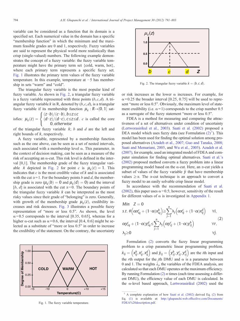
Fig. 2. The triangular fuzzy variable ~x ¼ b; c;dð Þ.


variable can be considered as a function that its domain is aspecified set. Each numerical value in the domain has a specific“membership function” in which the minimum and the maxi-mum feasible grades are 0 and 1, respectively. Fuzzy variablesare said to represent the physical world more realistically thancrisp (single-valued) numbers. The following example demon-strates the concept of a fuzzy variable: the fuzzy variable tem-perature might have the primary term set {cold, warm, hot},where each primary term represents a specific fuzzy set.Fig. 1 illustrates the primary term values of the fuzzy variabletemperature. In this example, temperature at −5 has member-ship in sets “warm” and “cold”.

The triangular fuzzy variable is the most popular kind offuzzy variable. As shown in Fig. 2, a triangular fuzzy variableis a fuzzy variable represented with three points (b,c,d). A tri-angular fuzzy variable ~x in R, denoted by (b,c,d), is a triangularfuzzy variable if its membership function μ~x : R→ 0;1½ � sat-

isfies: μ~x zð Þ ¼z−bð Þ= c−bð Þ; b≤z≤cd−zð Þ= d−cð Þ; c≤z≤d

0; otherwise

8<: . c is called the core

of the triangular fuzzy variable ~x; b and d are the left andright bounds of ~x, respectively.

A fuzzy variable, represented by a membership functionsuch as the one above, can be seen as a set of nested intervals,each associated with a membership level α. This parameter, inthe context of decision making, can be seen as a measure of therisk of accepting an α-cut. This risk level is defined in the inter-val [0,1]. The membership grade of the fuzzy triangular vari-able ~x depicted in Fig. 2 for point c is μ~x cð Þ ¼ 1. Thisindicates that c is the most credible value of ~x and is associatedwith the cut α=1. For the boundary points b and d, the member-ship grade is zero (μ~x bð Þ ¼ 0 and μ~x dð Þ ¼ 0) and the interval[b, d] is associated with the cut α=0. The boundary points ofthe triangular fuzzy variable ~x can be interpreted as the mostrisky values since their grade of “belonging” is zero. Generally,with growth of the membership grade μ~x zð Þ, credibility in-creases and risk decreases. Fig. 3 illustrates a possible fuzzyrepresentation of “more or less 0.5”. As shown, the levelα=0.5 corresponds to the interval [0.35, 0.65], whereas for ahigher α-cut such as α=0.6, the interval [0.4, 0.6] might be se-lected as a substitute of “more or less 0.5” in order to increasethe credibility of the statement. On the contrary, the uncertainty

1.00

0.50

0.25

0.00-15 -10 0 +10

Temperature(C)

Deg

ree

of

Mem

ber

ship

+15

HOTWARMCOLD

Fig. 1. The fuzzy variable temperature.

or risk increases as the lower α increases. For example, forα=0.25 the broader interval [0.25, 0.75] will be used to repre-sent “more or less 0.5”. Obviously, the maximum level of state-ment credibility (i.e. α=1) corresponds to the crisp number 0.5as a surrogate of the fuzzy statement “more or less 0.5”.

FDEA is a method for measuring and comparing the attrac-tiveness of a set of alternatives under condition of uncertainty(Lertworasirikul et al., 2003). Saati et al. (2002) proposed aDEA model which uses fuzzy data (see Formulation (2)1). Thismodel has been used for finding the optimal solution among pro-posed alternatives (Azadeh et al., 2007; Guo and Tanaka, 2008;Saati and Memariani, 2005, and Wu et al., 2005). Azadeh et al.(2007), for example, used an integratedmodel of FDEA and com-puter simulation for finding optimal alternatives. Saati et al.'s(2002) proposed method converts a fuzzy problem into a linearprogramming model based on the α-cut. Here, an α-cut yields asubset of values of the fuzzy variable ~y that have membershipvalues ≥α. The α-cut technique is an approach to convert afuzzy model to an easily solvable crisp linear model.

In accordance with the recommendation of Saati et al.(2002), this paper uses α=0.5; however, sensitivity of the resultfor different values of α is investigated in Appendix 1.

Min Z ¼ 0

s:t: θ αxciq þ 1−αð Þxbiq� �

≥Xnj¼1

λj αxcij þ 1−αð Þxdij� �

∀i;

αycrq þ 1−αð Þydrq≤Xnj¼1

λj αycrj þ 1−αð Þybrj� �

∀r;

λj≥0 ∀j:

ð2Þ

Formulation (2) converts the fuzzy linear programmingproblem to a crisp parametric linear programming problem.

~xij ¼ xbij; xcij; x

dij

� �and ~yrj ¼ ybrj; y

crj; y

drj

� �are the ith input and

the rth output for the jth DMU and α is a parameter between0 and 1. The weights λj, the variables of the FDEA analysis, arecalculated so that each DMUoperates at the maximum efficiency.By running Formulation (2) n times (each time assessing a differ-ent DMU), the efficiency value of each DMU is calculated. Inthe α-level based approach, Lertworasirikul (2002) used the

1 A complete explanation of how Saati et al. (2002) derived Eq. (2) fromEq. (1) is available at: http://ghapanchi.web.officelive.com/Documents/FDEA%20description.pdf.

http://ghapanchi.web.officelive.com/Documents/FDEA%20description.pdf

http://ghapanchi.web.officelive.com/Documents/FDEA%20description.pdf

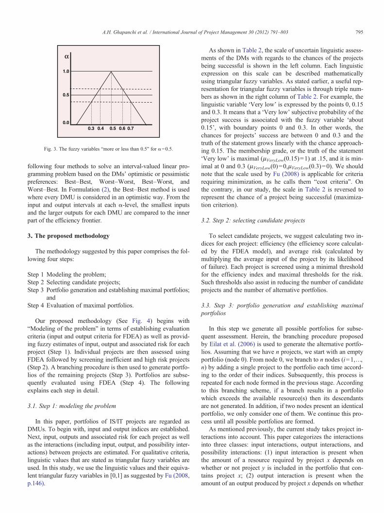
0.0

1.0

α

0.5

0.50.40.3 0.6 0.7

Fig. 3. The fuzzy variables “more or less than 0.5” for α=0.5.


following four methods to solve an interval-valued linear pro-gramming problem based on the DMs' optimistic or pessimisticpreferences: Best–Best, Worst–Worst, Best–Worst, andWorst–Best. In Formulation (2), the Best–Best method is usedwhere every DMU is considered in an optimistic way. From theinput and output intervals at each α-level, the smallest inputsand the larger outputs for each DMU are compared to the innerpart of the efficiency frontier.

3. The proposed methodology

The methodology suggested by this paper comprises the fol-lowing four steps:

Step 1 Modeling the problem;Step 2 Selecting candidate projects;Step 3 Portfolio generation and establishing maximal portfolios;

andStep 4 Evaluation of maximal portfolios.

Our proposed methodology (See Fig. 4) begins with“Modeling of the problem” in terms of establishing evaluationcriteria (input and output criteria for FDEA) as well as provid-ing fuzzy estimates of input, output and associated risk for eachproject (Step 1). Individual projects are then assessed usingFDEA followed by screening inefficient and high risk projects(Step 2). A branching procedure is then used to generate portfo-lios of the remaining projects (Step 3). Portfolios are subse-quently evaluated using FDEA (Step 4). The followingexplains each step in detail.

3.1. Step 1: modeling the problem

In this paper, portfolios of IS/IT projects are regarded asDMUs. To begin with, input and output indices are established.Next, input, outputs and associated risk for each project as wellas the interactions (including input, output, and possibility inter-actions) between projects are estimated. For qualitative criteria,linguistic values that are stated as triangular fuzzy variables areused. In this study, we use the linguistic values and their equiva-lent triangular fuzzy variables in [0,1] as suggested by Fu (2008,p.146).

As shown in Table 2, the scale of uncertain linguistic assess-ments of the DMs with regards to the chances of the projectsbeing successful is shown in the left column. Each linguisticexpression on this scale can be described mathematicallyusing triangular fuzzy variables. As stated earlier, a useful rep-resentation for triangular fuzzy variables is through triple num-bers as shown in the right column of Table 2. For example, thelinguistic variable ‘Very low’ is expressed by the points 0, 0.15and 0.3. It means that a ‘Very low’ subjective probability of theproject success is associated with the fuzzy variable ‘about0.15’, with boundary points 0 and 0.3. In other words, thechances for projects' success are between 0 and 0.3 and thetruth of the statement grows linearly with the chance approach-ing 0.15. The membership grade, or the truth of the statement‘Very low’ is maximal (μVeryLow(0.15)=1) at .15, and it is min-imal at 0 and 0.3 (μVeryLow(0)=0,μVeryLow(0.3)=0). We shouldnote that the scale used by Fu (2008) is applicable for criteriarequiring minimization, as he calls them “cost criteria”. Onthe contrary, in our study, the scale in Table 2 is reversed torepresent the chance of a project being successful (maximiza-tion criterion).

3.2. Step 2: selecting candidate projects

To select candidate projects, we suggest calculating two in-dices for each project: efficiency (the efficiency score calculat-ed by the FDEA model), and average risk (calculated bymultiplying the average input of the project by its likelihoodof failure). Each project is screened using a minimal thresholdfor the efficiency index and maximal thresholds for the risk.Such thresholds also assist in reducing the number of candidateprojects and the number of alternative portfolios.

3.3. Step 3: portfolio generation and establishing maximalportfolios

In this step we generate all possible portfolios for subse-quent assessment. Herein, the branching procedure proposedby Eilat et al. (2006) is used to generate the alternative portfo-lios. Assuming that we have n projects, we start with an emptyportfolio (node 0). From node 0, we branch to n nodes (i=1,…,n) by adding a single project to the portfolio each time accord-ing to the order of their indices. Subsequently, this process isrepeated for each node formed in the previous stage. Accordingto this branching scheme, if a branch results in a portfoliowhich exceeds the available resource(s) then its descendantsare not generated. In addition, if two nodes present an identicalportfolio, we only consider one of them. We continue this pro-cess until all possible portfolios are formed.

As mentioned previously, the current study takes project in-teractions into account. This paper categorizes the interactionsinto three classes: input interactions, output interactions, andpossibility interactions: (1) input interaction is present whenthe amount of a resource required by project x depends onwhether or not project y is included in the portfolio that con-tains project x; (2) output interaction is present when theamount of an output produced by project x depends on whether

Fig. 4. The proposed methodology.


or not project y is included in the portfolio that contains projectx; and (3) possibility interaction is present when the likelihoodof success for project x depends on whether or not project y isincluded in the portfolio that contains project x. For example,let's assume that cost is an input criterion and that we havetwo projects of x and y which would cost us $300,000 and$200,000 respectively. An input interaction of $ –50,000

between projects x and y means that by including both projectsin the same portfolio we could save $50,000 overall and pay$450,000 rather than $500,000.

After all possible portfolios are created, it is necessary to ac-cumulate the inputs and outputs of the projects which make upa particular portfolio. However, since this paper takes interac-tions between projects into consideration, accumulated inputs

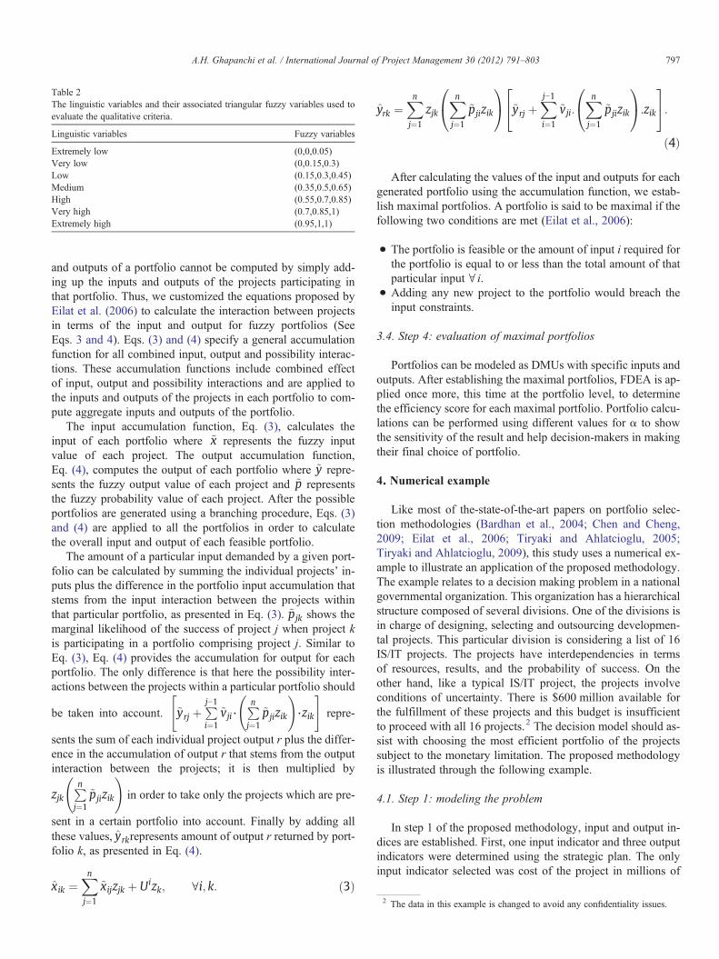
Table 2The linguistic variables and their associated triangular fuzzy variables used toevaluate the qualitative criteria.

Linguistic variables Fuzzy variables

Extremely low (0,0,0.05)Very low (0,0.15,0.3)Low (0.15,0.3,0.45)Medium (0.35,0.5,0.65)High (0.55,0.7,0.85)Very high (0.7,0.85,1)Extremely high (0.95,1,1)

2 The data in this example is changed to avoid any confidentiality issues.


and outputs of a portfolio cannot be computed by simply add-ing up the inputs and outputs of the projects participating inthat portfolio. Thus, we customized the equations proposed byEilat et al. (2006) to calculate the interaction between projectsin terms of the input and output for fuzzy portfolios (SeeEqs. 3 and 4). Eqs. (3) and (4) specify a general accumulationfunction for all combined input, output and possibility interac-tions. These accumulation functions include combined effectof input, output and possibility interactions and are applied tothe inputs and outputs of the projects in each portfolio to com-pute aggregate inputs and outputs of the portfolio.

The input accumulation function, Eq. (3), calculates theinput of each portfolio where ~x represents the fuzzy inputvalue of each project. The output accumulation function,Eq. (4), computes the output of each portfolio where ~y repre-sents the fuzzy output value of each project and ~p representsthe fuzzy probability value of each project. After the possibleportfolios are generated using a branching procedure, Eqs. (3)and (4) are applied to all the portfolios in order to calculatethe overall input and output of each feasible portfolio.

The amount of a particular input demanded by a given port-folio can be calculated by summing the individual projects' in-puts plus the difference in the portfolio input accumulation thatstems from the input interaction between the projects withinthat particular portfolio, as presented in Eq. (3). ~pjk shows themarginal likelihood of the success of project j when project kis participating in a portfolio comprising project j. Similar toEq. (3), Eq. (4) provides the accumulation for output for eachportfolio. The only difference is that here the possibility inter-actions between the projects within a particular portfolio should

be taken into account. ~yrj þPj−1i¼1

~vji⋅Pnj¼1

~pjizik

!⋅zik

" #repre-

sents the sum of each individual project output r plus the differ-ence in the accumulation of output r that stems from the outputinteraction between the projects; it is then multiplied by

zjkPnj¼1

~pjizik

!in order to take only the projects which are pre-

sent in a certain portfolio into account. Finally by adding allthese values, yrkrepresents amount of output r returned by port-folio k, as presented in Eq. (4).

xik ¼Xnj¼1

~xijzjk þ Uizk; ∀i; k: ð3Þ

yrk ¼Xnj¼1

zjkXnj¼1

~pjizik

0@

1A ~yrj þ

Xj−1i¼1

~vji:Xnj¼1

~pjizik

0@

1A:zik

24

35:ð4Þ

After calculating the values of the input and outputs for eachgenerated portfolio using the accumulation function, we estab-lish maximal portfolios. A portfolio is said to be maximal if thefollowing two conditions are met (Eilat et al., 2006):

• The portfolio is feasible or the amount of input i required forthe portfolio is equal to or less than the total amount of thatparticular input ∀ i.

• Adding any new project to the portfolio would breach theinput constraints.

3.4. Step 4: evaluation of maximal portfolios

Portfolios can be modeled as DMUs with specific inputs andoutputs. After establishing the maximal portfolios, FDEA is ap-plied once more, this time at the portfolio level, to determinethe efficiency score for each maximal portfolio. Portfolio calcu-lations can be performed using different values for α to showthe sensitivity of the result and help decision-makers in makingtheir final choice of portfolio.

4. Numerical example

Like most of the-state-of-the-art papers on portfolio selec-tion methodologies (Bardhan et al., 2004; Chen and Cheng,2009; Eilat et al., 2006; Tiryaki and Ahlatcioglu, 2005;Tiryaki and Ahlatcioglu, 2009), this study uses a numerical ex-ample to illustrate an application of the proposed methodology.The example relates to a decision making problem in a nationalgovernmental organization. This organization has a hierarchicalstructure composed of several divisions. One of the divisions isin charge of designing, selecting and outsourcing developmen-tal projects. This particular division is considering a list of 16IS/IT projects. The projects have interdependencies in termsof resources, results, and the probability of success. On theother hand, like a typical IS/IT project, the projects involveconditions of uncertainty. There is $600 million available forthe fulfillment of these projects and this budget is insufficientto proceed with all 16 projects.2 The decision model should as-sist with choosing the most efficient portfolio of the projectssubject to the monetary limitation. The proposed methodologyis illustrated through the following example.

4.1. Step 1: modeling the problem

In step 1 of the proposed methodology, input and output in-dices are established. First, one input indicator and three outputindicators were determined using the strategic plan. The onlyinput indicator selected was cost of the project in millions of


dollars (x1j). The output indicators include: the number ofpotential subsequent investments (y1j), contribution to thework-flow improvement (y2j), and percentage of contributionto electronic readiness (y3j). A probability of success Pj is alsoassociated with each project. Regarding the first output criterion,the managers of the organization under study who were involvedin developing their strategic plan preferred “the number of poten-tial subsequent investments” over “the total value of potentialsubsequent investments” because there was no significant differ-ence between the values of the available subsequent investments.With respect to the second output criterion, contribution to thework-flow improvement, a Likert scale (Likert, 1932) was used.Likert scale is a psychometric scale which is commonly used inquestionnaires. A Likert questionnaire item enables respondentsto specify their level of agreement with predefined answers(Likert, 1932). For our second output criterion, a seven-pointLikert scale was used (1= ‘extremely low’, 2= ‘very low’,3= ‘low’, 4= ‘medium’, 5= ‘high’, 6= ‘very high’, 7= ‘extremelyhigh’), and respondents were asked to pick one of these prede-fined options as their answer to the question posed on the secondoutput criterion (the extent to which running a given projectmay contribute to the improvement of the work-flow of thegovernment). For the second output criterion, y2j, linguisticvalues introduced in Table 2 were used. Table 3 shows inputand output indices of our decision making problem. It should benoted that these input and output indices are specific to the con-text of the example used in this study and are directly extractedfrom the strategic plan of the organization under study. Thus,one requirement of this methodology is the development ofinput and output criteria for any potential application.

After establishing the decision criteria, fuzzy values for theinput and output indicators as well as associated risk were esti-mated for each project. To do so, a group of 15 experts were in-vited and provided with a detailed description of each project,requirements of each project, and information about units ofcosts, man-hours, etc. Afterwards, the respondents received aquestionnaire to enter their estimates. The raw score for theinput, the outputs, the associated risk for each project, and the in-teractions (including input, output, and possibility interactions)among each pair of two projects were estimated by the expertsin a fuzzy manner. Subsequently, for each project, a symmetric

Table 3The decision making criteria used in the numerical example.

Datatype

Criterion Explanation

Input Cost The project costOutput Potential subsequent

projectsThe number of projects which their adoptionis contingent to this project's implementation

Work-flowimprovement

The degree of government work-flowimprovement based on a seven-point Likertscale (in addition to the reduction in resourcesand employees, and citizens' satisfaction)

E-readinesscontribution margin

The likeliness of citizens, businesses,government managers, employees, and otherstakeholders increasing their participation inthe IS/IT activities as a result of this project'simplementation

triangular fuzzy variable was computed for each input, output,and success probability criterion by averaging the values estimat-ed by the experts.

“Response stability” measures the stability across time bytesting whether or not respondents give the same answers tothe same questions over a period of time (Neuman, 2006). Inthis research, we used the test–retest method which has beenproposed as an efficient method for assessing the response sta-bility of respondents over a period of time (Neuman, 2006). Weasked the same questions from the same respondents twicewithin a nine month interval and computed the Pearson correla-tion coefficients for the responses. The Pearson correlation co-efficients for all the questions were greater than 0.7 indicating ahigh response stability of the questions.

The interactions among the input, outputs and probability ofsuccess are included in the interaction matrices. U representsthe input interaction matrix; (V1, V2, and V3) represent the out-puts interaction matrices, and P shows the probability interac-tion matrix (See Table 4). For each project, the average forinput, outputs, and success likelihood as well as its interactionswith other projects are listed in Table 4. In this table, ujk

i repre-sents the value interaction between project j and project k forinput i, Vr

jk shows the value interaction between project j andproject k for output r, and Pjk represents the marginal changein the success likelihood of project j when project k is partici-pating in a portfolio comprising project j. The project interac-tions are applicable after the portfolios are created in Step 3.

An example of the cost of project interaction would be the se-lection of both projects 7 and 8 which have some shared activi-ties. Since they share some resources, the total cost of the twoprojects would decrease by at least $12.6 million and at most$14 million. An example of potential subsequent projects inter-action would be including projects 3 and 4 in the same portfolio.Because there is a future project for which both are prerequisites,the sum of these two projects' number of potential subsequentprojects would increase by 1. Work-flow improvement interac-tion is seen if projects 7 and 8 that have synergy were simulta-neously selected, since they would then have a stronger effectand their accumulation improvement level would increase by0.15 on average. With respect to e-readiness, if projects 4 and 5that have synergy in benefits are selected in a portfolio, theyhave stronger impact, and their accumulation function onhuman resource e-readiness would increase by at least 7.1%, atmost 10.3%, and by 8.7% on average.

4.2. Step 2: selecting candidate projects

In order to have a manageable number of projects for the pur-pose of constructing and evaluating all possible portfolios of pro-jects, we performed an initial screening on each individual projectand weeded out projects with considerably low efficiency. To doso, we calculated two indices for each project: (i) the FDEA effi-ciency value for the project; and (ii) its average risk, calculated bymultiplying the average input of the project by its probability offailure. The data in Table 4 was used to calculate the FDEAscore for each individual project. The results are depicted inTable 5. Subsequently, through a minimal threshold for the

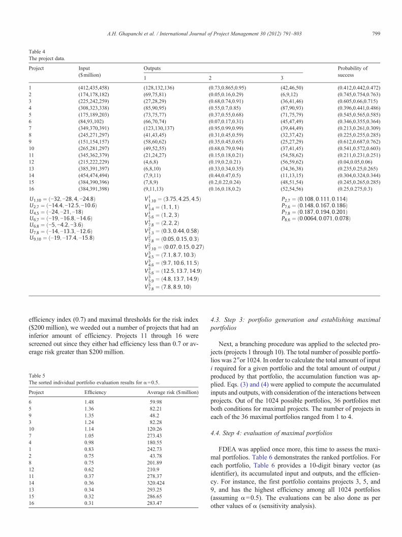
Table 4The project data.

Project Input($million)

Outputs Probability ofsuccess

1 2 3

1 (412,435,458) (128,132,136) (0.73,0.865,0.95) (42,46,50) (0.412,0.442,0.472)2 (174,178,182) (69,75,81) (0.05,0.16,0.29) (6,9,12) (0.745,0.754,0.763)3 (225,242,259) (27,28,29) (0.68,0.74,0.91) (36,41,46) (0.605,0.66,0.715)4 (308,323,338) (85,90,95) (0.55,0.7,0.85) (87,90,93) (0.396,0.441,0.486)5 (175,189,203) (73,75,77) (0.37,0.55,0.68) (71,75,79) (0.545,0.565,0.585)6 (84,93,102) (66,70,74) (0.07,0.17,0.31) (45,47,49) (0.346,0.355,0.364)7 (349,370,391) (123,130,137) (0.95,0.99,0.99) (39,44,49) (0.213,0.261,0.309)8 (245,271,297) (41,43,45) (0.31,0.45,0.59) (32,37,42) (0.225,0.255,0.285)9 (151,154,157) (58,60,62) (0.35,0.45,0.65) (25,27,29) (0.612,0.687,0.762)10 (265,281,297) (49,52,55) (0.68,0.79,0.94) (37,41,45) (0.541,0.572,0.603)11 (345,362,379) (21,24,27) (0.15,0.18,0.21) (54,58,62) (0.211,0.231,0.251)12 (215,222,229) (4,6,8) (0.19,0.2,0.21) (56,59,62) (0.04,0.05,0.06)13 (385,391,397) (6,8,10) (0.33,0.34,0.35) (34,36,38) (0.235,0.25,0.265)14 (454,474,494) (7,9,11) (0.44,0.47,0.5) (11,13,15) (0.304,0.324,0.344)15 (384,390,396) (7,8,9) (0.2,0.22,0.24) (48,51,54) (0.245,0.265,0.285)16 (384,391,398) (9,11,13) (0.16,0.18,0.2) (52,54,56) (0.25,0.275,0.3)

U1;10 ¼ −32;−28;4;−24:8ð ÞU2;7 ¼ −14:4;−12:5;−10:6ð ÞU4;5 ¼ −24;−21;−18ð ÞU6;7 ¼ −19;−16:8;−14:6ð ÞU6;8 ¼ −5;−4:2;−3:6ð ÞU7;8 ¼ −14;−13:3;−12:6ð ÞU9;10 ¼ −19;−17:4;−15:8ð Þ

V11;10 ¼ 3:75;4:25;4:5ð Þ

V13;4 ¼ 1;1;1ð Þ

V15;6 ¼ 1;2;3ð Þ

V17;8 ¼ 2;2;2ð Þ

V21;3 ¼ 0:3;0:44;0:58ð Þ

V27;8 ¼ 0:05;0:15;0:3ð Þ

V27;10 ¼ 0:07;0:15;0:27ð Þ

V34;5 ¼ 7:1;8:7;10:3ð Þ

V34;6 ¼ 9:7;10:6;11:5ð Þ

V35;6 ¼ 12:5;13:7;14:9ð Þ

V35;9 ¼ 4:8;13:7;14:9ð Þ

V37;8 ¼ 7:8;8:9;10ð Þ

P2;7 ¼ 0:108;0:111;0:114ð ÞP7;6 ¼ 0:148;0:167;0:186ð ÞP7;8 ¼ 0:187;0:194;0:201ð ÞP8;6 ¼ 0:0064;0:071;0:078ð Þ


efficiency index (0.7) and maximal thresholds for the risk index($200 million), we weeded out a number of projects that had aninferior amount of efficiency. Projects 11 through 16 werescreened out since they either had efficiency less than 0.7 or av-erage risk greater than $200 million.

Table 5The sorted individual portfolio evaluation results for α=0.5.

Project Efficiency Average risk ($million)

6 1.48 59.985 1.36 82.219 1.35 48.23 1.24 82.2810 1.14 120.267 1.05 273.434 0.98 180.551 0.83 242.732 0.75 43.788 0.75 201.8912 0.62 210.911 0.37 278.3714 0.36 320.42413 0.34 293.2515 0.32 286.6516 0.31 283.47

4.3. Step 3: portfolio generation and establishing maximalportfolios

Next, a branching procedure was applied to the selected pro-jects (projects 1 through 10). The total number of possible portfo-lios was 2nor 1024. In order to calculate the total amount of inputi required for a given portfolio and the total amount of output jproduced by that portfolio, the accumulation function was ap-plied. Eqs. (3) and (4) were applied to compute the accumulatedinputs and outputs, with consideration of the interactions betweenprojects. Out of the 1024 possible portfolios, 36 portfolios metboth conditions for maximal projects. The number of projects ineach of the 36 maximal portfolios ranged from 1 to 4.

4.4. Step 4: evaluation of maximal portfolios

FDEA was applied once more, this time to assess the maxi-mal portfolios. Table 6 demonstrates the ranked portfolios. Foreach portfolio, Table 6 provides a 10-digit binary vector (asidentifier), its accumulated input and outputs, and the efficien-cy. For instance, the first portfolio contains projects 3, 5, and9, and has the highest efficiency among all 1024 portfolios(assuming α=0.5). The evaluations can be also done as perother values of α (sensitivity analysis).

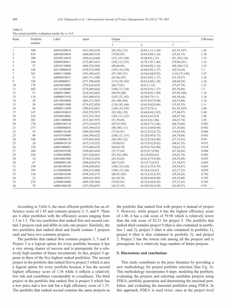
Table 6The sorted portfolio evaluation results for α=0.5.

Rank Portfolionumber

Label Input Output Efficiency

1 2 3

1 388 A0010100010 (551,585,619) (92,102,113) (0.83,1.11,1.54) (81,93,107) 1.452 418 A0010010010 (460,489,518) (75,85,95) (0.65,0.86,1.26) (53,62,73) 1.383 308 A0100110010 (584,614,644) (151,167,184) (0.48,0.8,1.23) (91,103,116) 1.354 164 A0000100011 (572,607,641) (102,113,125) (0.78,1.07,1.46) (79,90,101) 1.335 37 A0010110000 (484,524,564) (80,88,96) (0.64,0.86,1.16) (89,100,112) 1.336 148 A0110000010 (550,574,598) (103,116,130) (0.66,0.92,1.37) (42,52,64) 1.37 261 A0001110000 (543,584,625) (97,109,121) (0.44,0.68,0.92) (118,132,146) 1.278 21 A0000010011 (481,511,540) (85,96,107) (0.61,0.82,1.17) (51,59,67) 1.269 194 A0100000011 (571,596,620) (113,128,142) (0.62,0.88,1.28) (40,49,58) 1.2610 178 A0010010001 (574,616,658) (66,73,81) (0.8,1,1.33) (57,67,78) 1.2111 402 A0110100000 (574,609,644) (108,117,128) (0.65,0.92,1.27) (65,76,88) 1.212 51 A0000110001 (524,563,602) (90,99,108) (0.59,0.82,1.08) (87,96,106) 1.1813 114 A0000011010 (565,600,635) (103,122,142) (0.58,0.79,1.1) (45,54,64) 1.1614 28 A0110010000 (483,513,543) (91,100,109) (0.47,0.67,0.98) (42,51,60) 1.1415 58 A0100011000 (574,612,650) (126,145,166) (0.41,0.62,0.86) (35,43,53) 1.1116 84 A0000111000 (589,635,681) (108,125,143) (0.57,0.79,1) (81,92,103) 1.0817 147 A0001010010 (543,570,597) (92,106,120) (0.46,0.68,1.02) (75,86,97) 1.0818 516 A0100010001 (523,552,581) (101,111,122) (0.43,0.63,0.9) (40,47,54) 1.0619 282 A0011000000 (533,565,597) (51,59,68) (0.63,0.8,1.06) (56,67,78) 1.0520 770 A0000100110 (571,614,657) (85,95,105) (0.49,0.73,1.06) (66,76,86) 0.98321 275 A1000000010 (563,589,615) (88,100,111) (0.51,0.69,0.94) (33,39,46) 0.98322 54 A0000110100 (499,549,598) (75,83,91) (0.32,0.52,0.72) (76,85,94) 0.96423 40 A0101010000 (566,594,622) (108,121,135) (0.28,0.49,0.75) (64,74,84) 0.94124 546 A0100000110 (570,603,636) (96,109,122) (0.32,0.54,0.88) (27,35,43) 0.9425 24 A0000010110 (475,514,552) (70,80,91) (0.33,0.52,0.82) (40,47,55) 0.93226 338 A0001000001 (573,604,635) (60,69,79) (0.59,0.76,0.98) (54,63,72) 0.91927 264 A0010010100 (549,602,654) (51,57,64) (0.53,0.7,0.98) (47,56,66) 0.90428 530 A1000100000 (587,624,661) (93,101,109) (0.5,0.69,0.85) (56,63,70) 0.90329 14 A0010001000 (574,612,650) (43,52,63) (0.61,0.75,0.96) (30,39,48) 0.89330 67 A0000001100 (580,628,675) (60,72,85) (0.5,0.72,0.97) (31,38,47) 0.86931 150 A0100100100 (594,638,682) (100,110,120) (0.31,0.55,0.79) (50,59,67) 0.86332 294 A1100000000 (586,613,640) (104,115,126) (0.34,0.5,0.67) (22,27,33) 0.85933 138 A0100010100 (498,538,577) (86,95,105) (0.15,0.33,0.55) (29,36,42) 0.79234 23 A0000010101 (589,641,692) (61,69,76) (0.48,0.66,0.89) (45,52,60) 0.78535 278 A1000010000 (496,528,560) (76,83,91) (0.32,0.44,0.56) (33,37,41) 0.78536 70 A0001000100 (553,594,635) (43,51,59) (0.29,0.42,0.58) (42,49,57) 0.59


According to Table 6, the most efficient portfolio has an ef-ficiency score of 1.45 and contains projects 3, 5, and 9. Thereare 4 other portfolios with the efficiency scores ranging from1.3 to 1.5. The two portfolios that ranked first and second con-tain 3 projects each and differ in only one project. Similarly, thetwo portfolios that ranked third and fourth contain 3 projectseach and have two common projects.

The portfolio that ranked first contains projects 3, 5 and 9.Project 3 is a logical option for every portfolio because it hasa very strong chance of success and is prerequisite for a rela-tively high number of future investments. In fact, project 3 ap-pears in three of the five highest ranked portfolios. The secondproject in the portfolio that ranked first is project 5 which is alsoa logical option for every portfolio because it has the secondhighest efficiency score of 1.36 while it reflects a relativelylow risk and contributes considerably to e-readiness. The thirdproject in the portfolio that ranked first is project 9 which hasa low price and a low risk but a high efficiency score of 1.35.The portfolio that ranked second contains the same projects as

the portfolio that ranked first with project 6 instead of project5. However, while project 6 has the highest efficiency scoreof 1.48, it has a risk score of 59.98 which is relatively lowerthan the risk score of 82.21 for project 5. The portfolio thatranked third contains project 9 (that is also contained in portfo-lios 1 and 2), project 5 (that is also contained in portfolio 1),project 6 (that is also contained in portfolio 2), and project2. Project 2 has the lowest risk among all the projects and isprerequisite for a relatively large number of future projects.

5. Discussions and conclusions

This study contributes to the prior literature by providing anew methodology for project portfolio selection (See Fig. 4).This methodology incorporates 4 steps: modeling the problem;evaluating the projects and selecting candidate projects usingFDEA; portfolio generation and determining the maximal port-folios; and evaluating the maximal portfolios using FDEA. Inthis approach, FDEA is used twice: once at the project level


and once again at the portfolio level. A number of papers havesuggested different methodologies to evaluate portfolios of theprojects with interdependencies, while others have taken pro-ject uncertainty into consideration. However, there is a lack ofportfolio selection methods that concurrently incorporates pro-ject uncertainty and interdependencies. Hence, a key contribu-tion of this paper is the construction of a quantitativemethodology for selecting portfolios of projects that respondsto uncertainty conditions and deals with project interdepen-dencies in terms of resource, outcome and success probability.

Our study has two main managerial implications. Firstly, theportfolio selection methodology proposed in this study incorpo-rates project interdependencies. It implies that before makingany investment valuation decision, the project interactions interms of resources they use and outputs they produce shouldbe evaluated. This responds to IS/IT managers' concern whodo not typically consider the big picture of portfolio decisionproblems. Secondly, the methodology proposed in this paperprovides a rational basis for project portfolio selection. Thisstudy provides a decision model that objectively takes into ac-count immediate and future value of the projects.

The result of this research demonstrated some preferences ofapplying FDEA for portfolio selection. Firstly, the FDEA ofthis study generates a higher number of feasible portfolios com-pared with the DEA proposed by prior research (e.g. Eilat et al.,2006). This offers the opportunity to examine more portfolios,which becomes an advantage for FDEA. Secondly, FDEA isable to take uncertainty conditions into account (other tech-niques such as DEA just uses rigid estimates). Thirdly, employ-ing FDEA for portfolio selection ameliorates the deficiency ofDEA in differentiating among the most efficient portfolios.

Several methodologies proposed by prior studies on portfo-lio selection and evaluation are not able to suggest a single‘best’ portfolio; rather, they reduce several potential portfoliosof projects to a handful of portfolios, presumably of equal‘value’. The decision methodology proposed here is able to de-termine the optimal portfolio (given the set of establishedcriteria). By using this methodology, decision makers will beable to select the most efficient portfolio(s). In other words,not only does the proposed methodology assist decision makersin eliminating inefficient portfolios, it also helps them choosethe most efficient ones.

Table 7The top ten portfolios for α=0, 0.25, 0.5 and 0.75.

Rank α=0 α=0.25

Portfolio number Attractiveness Portfolio number Attractiveness

1 388 2.2426 388 1.83872 418 2.1906 418 1.79573 164 2.0964 308 1.75814 37 2.0881 164 1.74445 308 2.0866 37 1.73496 148 2.047 148 1.6867 261 2.0277 261 1.66978 402 2.0190 21 1.64449 21 1.9985 402 1.634810 194 1.8379 194 1.5644

6. Limitations and future work

The following are the limitations of the method proposed inthis study:

• The total number of possible portfolios to be evaluated by theproposed methodology is 2n (n is the number of candidateprojects). In this study, we used 10 candidate projects and enu-merated 210=1024 portfolios. However, if the number of can-didate projects increases, the method becomes less efficient.Assuming that we have 20 candidate projects, the total numberof possible portfolios would be 220=1,048,576. It is not prac-tical to evaluate this many portfolios. Therefore, it is necessaryto perform an initial screening to identify a manageable num-ber of projects to be used in the portfolio construction process.

• Including three or more projects in a portfolio may require a re-source input for the portfolio that is significantly smaller thanthe sum of the inputs required for each project individually orfor the projects considered in pairs. The additional project(s) in-

creases the number of alternative portfolios fromn2

� �¼

n n−1ð Þ=2 tonk

� �¼ n!=k! n−kð Þ!. If n=10 and k=4, the

number of alternative portfolios increases from 45 to 180; butif k can assume any value, including all 10 projects in onelarge portfolio, the number of alternative portfolios increasesto 210=1024.

• The proposed model copes only with pair-wise interactionsbetween projects in input, output, and the chance of success.Therefore, an avenue for future research would be to takeinto account multiple interactions. If we only consider pair-wise interactions between the projects, the number of inter-

actions we need to analyze would ben2

� �¼ n n−1ð Þ=2.

However, if we consider k_way interactions (kN2), weshould also take into account 2_, 3_, …, k−1_ way interac-tions. In other words, if n=10 and k=3, we need to analyzen2

� �þ n

3

� �¼ 45þ 120 ¼ 165 interactions. Therefore,

one avenue of future research would be to consider triple-wise interactions or even higher interactions (i.e. situations

α=0.5 α=0.75

Portfolio number Attractiveness Portfolio number Attractiveness

388 1.45 388 1.2315418 1.38 308 1.2166308 1.35 418 1.2161164 1.33 164 1.207137 1.33 37 1.2029

148 1.3 178 1.1552261 1.27 148 1.137121 1.26 261 1.1354

194 1.26 194 1.1316178 1.21 51 1.1315

Attractiveness of feasible portfolios for each α

0

0.5

1

1.5

2

2.514 21 23 24 28 37 40 51 54 58 67 70 84 114

138

147

148

150

164

178

194

261

264

275

278

282

294

308

338

388

402

418

516

530

546

770

Portfolio #

Att

ract

iven

ess

valu

e

α=0 α=0.25 α=0.5 α=0.75

Fig. 5. The efficiency of feasible portfolios for α=0, 0.25, 0.5 and 0.75.


in which more than two projects have an interaction effect;for example, where including projects x, y, and z whichhave an interaction with respect to input i in a portfolio re-sults in the total value of input i required for the portfolioto be different from the sum of input i required for each pro-ject individually).

In the example provided in this paper, we only consideredthe mean values and disregarded the variance since the re-sponses returned by the experts did not vary significantly. Weconsider this acceptable because the focus of this paper wasin introducing a methodology that can assist in selecting portfo-lios of projects (given a set of input, output, and success possi-bility indices); the way in which estimates for these indices arecomputed for each project was not the focus of this study.

More research is needed to examine the effects of project inter-actions and interrelationships. Further research is also requiredwith respect to the qualitative aspects of IS/IT project selection.The problem of quantifying the qualitative factors remains a dif-ficult and sometimes controversial task. For example, we used theLikert scale to assign numbers to linguistic evaluations. But thelinguistic evaluations are not subject to the same rules of algebraas numbers on the real line because they do not obey the same ax-ioms. Researchers and practicing managers must be careful not toaccept the resulting ‘numbers’ thoughtlessly. (An autistic boymay score 10 on geometry and 0 on social behavior, but the aver-age of 5 has no meaning whatsoever!)

Acknowledgment

The authors would like to express their gratitude to the anon-ymous reviewers whose constructive and insightful commentshave led to many improvements in this paper.

Appendix 1. Sensitivity analysis

The results presented in Tables 5 and 6 were based onα=0.5 in Eq. (2). In a sensitivity analysis, we studied the ef-fects of different α values, namely α=0, 0.25 and 0.75. Thetop ten portfolios for each α and their associated efficiencyscores are shown in Table 7. The efficient portfolios for eachα are relatively similar. For instance, portfolio 388 which in-cludes projects 3, 5, and 9 is the most efficient portfolio foreach value of α. Most importantly, portfolios 388, 418, 164,

308, and 37 are the top five portfolios for each α value. Accord-ing to Fig. 5, the efficiency curve of the feasible portfolios fordifferent α values is very similar. For example, portfolios 388and 70 have the maximum and minimum amount of efficiencyscores for each value of α studied in this sensitivity analysis.

References

Azadeh, M.A., Anvari, M., Izadbakhsh, H., 2007. An integrated FDEA-PCAmethod as decision making model and computer simulation for system. Pro-ceedings of the Summer Computer Simulation.

Bacon, C.J., 1992. The use of decision criteria in selecting information systems/technology investments. MIS Quarterly 335–353 September.

Baker, N., Freeland, J., 1975. Recent advances in R&D benefit measurementand project selection methods. Management Science 21, 1164–1175.

Bard, J.F., Balachandra, R., Kaufmann, P.E., 1988. An interactive approach toR&D project selection and termination. IEEE Transactions on EngineeringManagement EM 35, 139–146.

Bardhan, I., Bagchi, S., Sougstad, R., 2004. Prioritizing a portfolio of informa-tion technology investment projects. Journal of Management InformationSystems 21 (2), 33–60.

Basso, A., Peccati, L.A., 2001. Optimal resource allocation with minimum ac-tivation levels and fixed costs. European Journal of Operational Research131, 536–549.

Charnes, A., Cooper, W.W., Rhodes, E., 1978. Measuring the efficiency of de-cision making units. European Journal of Operational Research 2, 429–444.

Chen, C.T., Cheng, H.L., 2009. A comprehensive model for selecting informa-tion system project under fuzzy environment. International Journal ofProject Management 27, 389–399.

Coffin, M.A., Taylor, B.W., 1996. Multiple criteria R&D project selection andscheduling using fuzzy logic. Computers & Operations Research 23 (3),207–220.

Cooper, R.G., Edgett, S.J., Kleinshmidt, E.J., 1997. Portfolio Management forNew Products. McMaster University, Hamilton, ON.

Danila, N., 1989. Strategic evaluation and selection of R&D projects. R&DManagement 19, 47–62.

Dickinson, M.W., Thornton, A.C., Graves, S., 2001. Technology portfolio man-agement: optimizing interdependent projects over multiple time periods.IEEE Transactions on Engineering Management 48, 518–527.

Eilat, H., Golany, B., Shtub, A., 2006. Constructing and evaluating balancedportfolios of R&D projects with interactions: a DEA based methodology.European Journal of Operational Research 172, 1018–1039.

Farbey, B., Land, F., Target, D., 1993. How to Assess Your IT Investment.Butterworth Heinemann.

Farbey, B., Land, F., Targett, D., 1999. Moving IS evaluation forward: learningthemes and research issues. Journal of Strategic Information Systems 8 (2),189–207.

Fu, G., 2008. A fuzzy optimization method for multicriteria decision making: anapplication to reservoir flood control operation. Expert Systems with Appli-cations 34 (1), 145–149.


Gunasekarana, A., Love, P.E.D., Rahimic, F., Miele, R., 2001. A model for in-vestment justification in information technology projects. InternationalJournal of Information Management 21, 349–364.

Guo, P., Tanaka, H., 2008. Decision making based on fuzzy data envelopmentanalysis. Intelligent Decision and Policy Making Support Systems. Springer-Verlag, Berlin Heidelberg, pp. 39–54.

Henriksen, A.D., Traynor, A.J., 1999. A practical R&D project-selection scor-ing tool. IEEE Transactions on Engineering Management 46, 158–170.

Huang, C.C., Chu, P.Y., Chiang, Y.H., 2008. A fuzzy AHP application ingovernment-sponsored R&D project selection. Omega 36 (6), 1038–1052.

Irani, Z., Sharif, A., Love, P.E.D., Kahraman, C., 2002. Applying concepts offuzzy logic cognitive mapping to model: the IT/IS investment evaluationprocess. International Journal of Production Economics 75, 199–211.

Lertworasirikul, S. 2002. Fuzzy data envelopment analysis in supply chainmodeling and analysis, Ph.D. Dissertation, Department of Industrial Engi-neering, North Carolina State University.

Lertworasirikul, S., Fang, S.C., Nuttle, H.L.W., Joines, J.A., 2003. Fuzzy BCCmodel for data envelopment analysis. Fuzzy Optimization and DecisionMaking 2 (4), 337–358.

Likert, R., 1932. A technique for the measurement of attitudes. Archives ofPsychology 140, 1–55.

Lin, C.H., Hsieh, P.J., 2004. A fuzzy decision support system for strategic port-folio management. Decision Support Systems 38 (3), 383–398.

Møen, J., 2005. Is mobility of technical personnel a source of R&D spillovers?Journal of Labor Economic 23 (1), 81–114.

Neuman, W.L., 2006. Social research methods, Pearson International Edition, 6Edition.

Ravanshadnia, M., Rajaie, H., Abbasian, H.R., 2010. Hybrid fuzzy MADMproject-selection model for diversified construction companies. CanadianJournal of Civil Engineering 37 (8), 1082–1093.

Ravanshadnia, M., Rajaie, H., Abbasian, H.R., 2011. A comprehensive bid/no-biddecision making framework for construction companies. Iranian Journal ofScience and Technology Transaction B-Engineering 35 (C1), 95–103.

Rivard, S., Raymond, L., Verreault, D., 2006. Resource-based view and competi-tive strategy: an integrated model of the contribution of information technolo-gy to firm performance. Journal of Strategic Information Systems 15, 29–50.

Saati, S., Memariani, A., 2005. Reducing weight flexibility in fuzzy DEA.Applied Mathematics and Computation 161, 611–622.

Saati, M., Memariani, A., Jahanshahloo, G.R., 2002. Efficiency analysis andranking of DMUs with fuzzy data. Fuzzy Optimization and Decision Making1, 255–267.

Schmidt, R.L., 1993. A model for R&D project selection with combined bene-fit, outcome and resource interactions. IEEE Transactions on EngineeringManagement 40, 403–410.

Tiryaki, F., Ahlatcioglu, B., 2005. Fuzzy stock selection using a new fuzzyranking and weighting algorithm. Applied Mathematics and Computation170 (1), 144–157.

Tiryaki, F., Ahlatcioglu, B., 2009. Fuzzy portfolio selection using fuzzy analytichierarchy process. Information Sciences 179 (1–2), 53–69.

Verma, D., Sinha, K.K., 2002. Toward a theory of project interdependencies inhigh tech R&D environments. Journal of Operations Management 20,451–468.

Wang, J., Hwang, W.L., 2007. A fuzzy set approach for R&D portfolio selec-tion using a real options valuation model. Omega 35, 247–257.

Wu, L.C., Ong, C.S., 2008. Management of information technology investment:a framework based on a real options and mean–variance theory perspective.Technovation 28, 122–134.

Wu, R., Yong, J., Zhang, Z., Liu, L., Dai, K., 2005. A game model for selectionof purchasing bids in consideration of fuzzy values. Proceedings ServicesSystems and Services Management.