comparing meaning in language and cognition: p-hyponymy ... › people › bob.coecke ›...
TRANSCRIPT

Comparing Meaning in Languageand Cognition:
P-Hyponymy, ConceptCombination, Asymmetric
Similarity
Candidate number: 123 893
University of Oxford
A thesis submitted for the degree of
MSc in Mathematics and Foundations of Computer Science
Trinity 2015

This thesis is dedicated tomy parents Albena and Yordan.

Abstract
In this dissertation we work in the framework of compositional distributional models ofmeaning to examine a number of asymmetric linguistic phenomena that manifest them-selves in language and cognition. These include overextension with respect to conceptcombination, asymmetry of similarity judgment and hyponymy and typicality. In partic-ular, we make use of the formalism of density matrices, which were recently introduced asan alternative to the vector-based model of word meaning. We first consider the formertwo of the above-mentioned phenomena using only tools that have been developed so farin the distributional compositional model. We then proceed to define a new quantitativeasymmetric measure on density matrices, called p-hyponymy, which allows us to deter-mine the strength of hyponymy in hyponym-hypernym pairs. We show how this can belifted to the level of the sentence structures that our mathematical model of meaningsupports and consider the implications of this result. We conclude with a brief discussionof how this measure can potentially be modified to account for other similar phenomena.

Contents
1 Introduction 11.1 Background . . . . . . . . . . . . . . . . . . . . . . . . . . . . . . . . . . . . . . . . . . 11.2 Overview and new contributions . . . . . . . . . . . . . . . . . . . . . . . . . . . . . . 2
2 A compositional distributional model of meaning 42.1 Types and distributions. Grammar and meaning. . . . . . . . . . . . . . . . . . . . . . 4
2.1.1 Pregroup Grammars . . . . . . . . . . . . . . . . . . . . . . . . . . . . . . . . . 42.1.2 Finite dimensional Hilbert spaces . . . . . . . . . . . . . . . . . . . . . . . . . . 6
2.2 Category theoretic and graphical calculus framework for DisCoCat . . . . . . . . . . . 72.2.1 What is a category? . . . . . . . . . . . . . . . . . . . . . . . . . . . . . . . . . 72.2.2 Monoidal categories . . . . . . . . . . . . . . . . . . . . . . . . . . . . . . . . . 72.2.3 Compact closed categories . . . . . . . . . . . . . . . . . . . . . . . . . . . . . . 11
2.3 Uniting syntax and semantics via a compact closed category . . . . . . . . . . . . . . . 132.3.1 Pregroup grammars as compact closed categories . . . . . . . . . . . . . . . . . 132.3.2 Finite dimensional Hilbert spaces as compact closed categories . . . . . . . . . 142.3.3 Meanings of sentences . . . . . . . . . . . . . . . . . . . . . . . . . . . . . . . . 15
2.4 Relative clauses via Frobenius algebras . . . . . . . . . . . . . . . . . . . . . . . . . . . 182.4.1 Relative pronouns via Frobenius algebras . . . . . . . . . . . . . . . . . . . . . 19
2.5 Concrete vector spaces for nouns and sentences . . . . . . . . . . . . . . . . . . . . . . 212.5.1 Truth-theoretic meaning . . . . . . . . . . . . . . . . . . . . . . . . . . . . . . . 212.5.2 A more distributional approach to word meaning and a new sentence space . . 22
3 The CPM construction and density matrix formalism 243.1 The doubling construction and CPM . . . . . . . . . . . . . . . . . . . . . . . . . . . . 24
3.1.1 The doubling construction on †-compact closed categories . . . . . . . . . . . . 243.1.2 The subcategory CPM(C) of D(C) . . . . . . . . . . . . . . . . . . . . . . . . . 263.1.3 Sentence meaning in the category CPM(C) . . . . . . . . . . . . . . . . . . . . 28
3.2 Modeling word and sentence meaning in CPM(FHilb) . . . . . . . . . . . . . . . . . . 293.2.1 Density matrices as states in CPM(FHilb) . . . . . . . . . . . . . . . . . . . . 293.2.2 Using density matrices to model word meanings . . . . . . . . . . . . . . . . . 30
4 Applications of distributional compositional models to cognitive linguistics phe-nomena 324.1 Concept combination and the Pet Fish phenomenon . . . . . . . . . . . . . . . . . . . 32
4.1.1 What is concept combination? . . . . . . . . . . . . . . . . . . . . . . . . . . . 324.1.2 Overextension, the Pet Fish phenomenon and the shortfalls of fuzzy set theory 334.1.3 Concept combination in a vector-based DisCoCat . . . . . . . . . . . . . . . . . 334.1.4 Transition to a density-matrix based environment in CPM(FHilb) . . . . . . . 35
4.2 Asymmetry of similarity judgments . . . . . . . . . . . . . . . . . . . . . . . . . . . . . 364.2.1 Similarity is not symmetric . . . . . . . . . . . . . . . . . . . . . . . . . . . . . 364.2.2 DisCoCat model to capture asymmetry . . . . . . . . . . . . . . . . . . . . . . 37
i

5 P-Hyponymy 405.1 Introduction . . . . . . . . . . . . . . . . . . . . . . . . . . . . . . . . . . . . . . . . . . 40
5.1.1 What is hyponymy? . . . . . . . . . . . . . . . . . . . . . . . . . . . . . . . . . 405.1.2 Graded hyponymy . . . . . . . . . . . . . . . . . . . . . . . . . . . . . . . . . . 405.1.3 Using measures on density matrices for hyponymy . . . . . . . . . . . . . . . . 415.1.4 Properties of hyponymy . . . . . . . . . . . . . . . . . . . . . . . . . . . . . . . 41
5.2 Background definitions and results . . . . . . . . . . . . . . . . . . . . . . . . . . . . . 415.3 P-Hyponyms . . . . . . . . . . . . . . . . . . . . . . . . . . . . . . . . . . . . . . . . . 42
5.3.1 A new measure on density matrices . . . . . . . . . . . . . . . . . . . . . . . . . 425.3.2 Interpretation of the values of p . . . . . . . . . . . . . . . . . . . . . . . . . . 425.3.3 Extracting p-hyponymy values out of hyponym-hypernym pairs . . . . . . . . . 435.3.4 Properties of P-Hyponymy . . . . . . . . . . . . . . . . . . . . . . . . . . . . . 45
5.4 P-Hyponymy lifted to the level of sentences . . . . . . . . . . . . . . . . . . . . . . . . 475.4.1 P-Hyponymy in positive transitive sentences . . . . . . . . . . . . . . . . . . . 475.4.2 P-Hyponymy in relative clauses . . . . . . . . . . . . . . . . . . . . . . . . . . . 535.4.3 General case of P-Hyponymy . . . . . . . . . . . . . . . . . . . . . . . . . . . . 56
5.5 Using the same idea for other applications . . . . . . . . . . . . . . . . . . . . . . . . . 58
6 Conclusion and future directions 60
Bibliography 62
ii

Chapter 1
Introduction
1.1 Background
Faithfully representing meaning in natural languages using mathematical formalism is one of the mostchallenging questions in linguistics and computer science. The practical gains of acquiring a deeperformal understanding of language include improvements to tasks such as machine translation, docu-ment retrieval and search optimisation, among others. On the theory front, the process of developingand exploring mathematical structures that better capture language has the potential to further ourunderstanding of cognition and intelligence.
Computers are very good at tasks that involve words existing in a vacuum, but when these wordsare put together into larger grammatical units, such as sentences, they fail to produce the same high-quality results. The main problem is that sentences are not simply concatenations of words in whicheven the word order is irrelevant. In fact, there is a very deep connection between the meaning of asentence, the meaning of its words, and the grammar that propagates through it in order to outputa coherent whole. We humans excel at deducing meanings of sentences we have never seen before bysimply drawing upon our knowledge of grammar and vocabulary. This, it turns out, is an incrediblycomplex task for a computer.
Two orthogonal solutions to this problem have been explored over the years. The more traditionalapproach [27] is built upon concepts from classical mathematical logic and adheres to the principleof compositionality [30], which tells us that the meaning of a sentence is a function of the syntacticrelationships of the words comprising it. Basic grammatical types are assigned to words, which arerepresented as elements in an algebraic structure such as a Lambek grammar or pregroup [23, 24],and interactions between words are achieved via the binary operation with which the structure isequipped. This method, however, completely disregards the actual meanings of words.
This leads us to the second and much more recent approach, the distributional one, which is basedon Firth’s dictum that ‘You shall know a word by the company it keeps’ [8]. In this model, words arerepresented via vectors, usually from high-dimensional vector spaces whose basis elements correspondto relevant context features. These are normally extracted from a large body of text such a corpus.The idea behind representing words in terms of other co-occurring words lies in the assumption thatmeaning is based entirely on contextual co-occurrence. This approach has proved to be very useful inpractical applications, but has very limited theoretical value and does not provide us with the wholepicture either.
To sum up, the main di↵erence between the compositional and the distributional models of meaningis that the former is qualitative and theoretical, while the latter is quantitative and practical. Neitherof them is capable of fully capturing meaning. The quest for finding a more complete mathematicalframework for the natural language problem has led in recent years to the development of a newmodel, unifying the above-mentioned ones. First introduced in [4] and formalised in [7], the so-calleddistributional compositional categorical (DisCoCat) model of meaning unites the structures used inthe compositional and the distributional approach, namely pregroups and finite dimensional vector
1

spaces, via category theory and draws inspiration from concepts, ideas, results and formalism fromquantum information theory.
In this model, the meaning of a string of words is computed via a categorical morphism extractedfrom the grammar of this string and applied to the tensor product of the vectors corresponding toits functional words. Upon application, these so-called meaning maps give an output of the form ofa vector and vectors corresponding to meanings of structures of the same grammatical type alwayslive in the same vector space. This enables us to compare meanings above the word level using thesame similarity measures as for words, such as the vector cosine. However, in many cases in languageand in phenomena from cognitive linguistics, asymmetry in similarity is prevalent. Prototypicalityand hyponymy, asymmetry of similarity judgments and overextension with respect to concept combi-nation are just some of the examples where making comparisons under the assumption of symmetryfails to produce adequate results.
In this dissertation we will attempt to utilise the DisCoCat framework developed so far, including itsrecent extension that allows the use of vectors to be replaced by density matrices, to model asymmetryin a number of di↵erent scenarios. Work in the area has only recently began with [2,32,33] and thereis still a lot of room for the development of various approaches to capturing hyponymy, entailment,prototypicality and many other intrinsically asymmetric phenomena.
1.2 Overview and new contributions
We begin Chapter 2 with an overview of the mathematical framework behind the distributional com-positional model of meaning of [7]. We first introduce pregroup grammars and finite dimensionalHilbert spaces as standalone structures, while simultaneously outlining their use in modeling syntaxand semantics, respectively. We then proceed to establish the connection between the two via thecommon language of category theory. We define the categories Preg and FHilb, which are both ex-amples of the so-called compact closed categories that come equipped with a very intuitive graphicalcalculus, allowing us to reduce equational expressions within the categories to simple diagrammaticmanipulations. We show how the structural morphisms of the categories give rise to sentence meaningmaps and examine the additional structure provided by the Frobenius algebras for capturing meaningof relative clauses [34, 35].
The development of the so-called CPM construction in categories has led to recent advancementsin the field whereby density matrices are used in place of vectors for word meaning [2, 32, 33]. Thisis achieved by passing from the category FHilb to CPM(FHilb), which is also a †-compact closedcategory. In Chapter 3, we outline the general framework of the CPM construction and considerhow meaning maps can be interpreted in this setting and what the advantages of working with den-sity matrices are. In brief, density matrices showcase more clearly the di↵erence between mixingand correlation of features, similar to their role in quantum computing. In addition, they possessa richer structure that enables us to consider various measures of similarity that vectors do not admit.
We begin Chapter 4 with a brief discussion of a couple of linguistic phenomena from psychology andcognition, namely the problem of overextension with respect to concept combination [17] and asym-metry of similarity judgment [40]. While these phenomena have been around for a long time, thereis still a lot of room for improvement in terms of the mathematical models used to capture them.Recent work [25] has shown some promise in applying the DisCoCat model to represent overextensionvia the traditional vector-based approach by taking into account the grammatical structure of theindividual concepts that comprise a combined unit. Here we extend upon this work to show howdensity matrices can be used for the same task. We then go on to show how asymmetry in measuringthe similarity between a more prototypical concept and another concept from the same category canbe represented by using the intrinsic asymmetry of verbs such as is similar to and the compositonalityof the meaning map. We come back to the same phenomenon in Chapter 5 and consider a di↵erentapproach in which the need for an explicit verb is eliminated and concepts are represented via densitymatrices.
2

One of the main advantages of transitioning to the CPM(FHilb) category and using density matricesinstead of vectors lies in the opportunity for defining various asymmetric measures on the matrices.These in turn give rise to orderings that can be utilised in tasks such as hypernym-hyponym classifi-cation. We define a new very simple and intuitive measure on density matrices, called p-hyponymy,that allows us to extract quantitative information about the relative strength of a given hyponym-hypernym bond. We show how this link manifests itself at the sentence level in a variety of di↵erentsentence structures. Finally, we briefly discuss the possibility of implementing variations of this mea-sure to the task of modeling linguistic phenomena other than hyponymy, such as those from Chapter4.
3

Chapter 2
A compositional distributionalmodel of meaning
In their paper [7], Coecke, Sadrzadeh and Clark first establish the category-theoretic framework fora new model of meaning that aims to unite the two standard approaches to capturing the structureof natural languages - the compositional and the distributional one. At first sight the use of categorytheory - a field which is often a↵ectionately referred to as ‘general abstract nonsense’ - to modela natural language may seem a bit surprising. However, its suitability for this purpose is easy toobserve. It enables us to model syntax and semantics separately in two di↵erent categories which,via their shared structural identities, allow us to derive sentence meanings in a way that takes intoaccount grammar and individual word meanings simultaneously.
In more concrete terms, we store qualitative information about word meanings in the category FHilband information about syntax in the category Preg and achieve the transition from the latter to theformer via a strongly monoidal functor Preg ! FHilb.
Moreover, the structural morphisms provided by the compact closed category allow us to computemaps which can be applied to strings of words to produce their combined meaning. This can be usednot only for the purposes of establishing whether or not a sentence is true or false (as in Montaguesemantics) but also to extract richer information about it, depending on what we aim to achieve andwhat data we are interested in obtaining.
This chapter serves as an introduction and overview of the categorical framework used in the distri-butional compositional categorical (DisCoCat) model and the applications to extracting meaning outof various structures, such as positive transitive sentences and relative clauses.
2.1 Types and distributions. Grammar and meaning.
2.1.1 Pregroup Grammars
In 1958 [22] J. Lambek introduced a syntactic calculus that formalises the grammatical structureof language and later on built upon this work by making use of the mathematical formalism ofpregroups [23]. Below we give a brief overview of how pregroup grammars can be used to capturesyntax and grammatical reductions. For a more detailed account of the use of types as elements of apregroup and applications, see [21, 24].
Definition 1 (Partially ordered monoid). A partially ordered monoid (P , , · , 1) is a partiallyordered set (P , ) together with an associative binary operation · : P ⇥ P ! P called monoidmultiplication, and a unit element 1, and such that the multiplication is order-preserving:
(p q) =) (r·p r·q) ^ (p·r q·r) 8 p, q, r 2 P.
Definition 2 (Pregroup algebra). A pregroup algebra�P , , · , 1 , (�)l , (�)r
�is a partially ordered
monoid together with two unary operations (�)l : P ! P and (�)r : P ! P called the left and right
4

adjoint respectively, such that for each p 2 P there exist pl, pr 2 P satisfying:
pl·p 1 p·plp·pr 1 pr·p.
Adjoints are unique and satisfy the following properties [7]:
1. Order-reversing: (p q) =) (qr pr) ^ (ql pl) ;
2. Opposite adjoints annihilate: (pr)l = p = (pl)r ;
3. Self-adjoint unit and multiplication: 1r = 1 = 1l and ((p·q)r = qr·pr) ^ �(p·q)l = ql·pl� .Definition 3 (Pregroup grammar [33]). A pregroup grammar G =
�P , , · , 1 , (�)l , (�)r
�is a
pregroup algebra which is freely generated over a set of basic types B that includes an end type and atype dictionary which associates pregroup elements to the vocabulary of a (natural) language.
Note that we say that a pregroup P is freely generated over a set B to mean that all the elements ofP can be formed out of the elements of B via zero or more applications of the monoid operation andthe adjoint operators (�)r and (�)l.
In the context of natural languages B is often taken to be the set B = {n, s, j,�}, where n is the typeassigned to nouns by the type dictionary; j is the the type of infinitives of verbs; � is a gluing type,and s is the type of a declarative statement. We also call the type s the end type of this grammar.For the rest of this dissertation the pregroup grammar G will be understood to mean exactly thegrammar that is freely generated over the set B above.
The following remarks, terminology and conventions will become useful later on:
• The grammatical type of a string of words is the concatenation (i.e. the monoidal multiplica-tion) of the types of the individual words in the string in the order in which they appear. Thisis an element of G.
• We can often simplify a grammatical type by using the properties of adjoints and the associa-tivity of the monoidal operation. We call such a simplification a reduction. When a stringx 2 G can be reduced to some other string y 2 G we write ‘x y’ or ‘x ! y’. I will usethese interchangeably. This notion will be made more precise once compact closed categoriesare introduced.
• A well-typed or grammatical sentence is a sentence whose grammatical type reduces to theend type s.
• A well-typed noun phrase is is a phrase or a sentence whose grammatical type reduces tothe basic type n.
The most important functional words that we will need here are transitive and intransitive verbs,adjectives and various pronouns. Thus, we summarise their types below, following the conventionsof [34, 35].
functional word type
transitive verb nrsnl
intransitive verb nrsadjective nnl
subject relative pronoun (who, which, that) nrnslnobject relative pronoun (whom, which, that) nrnnllsl
subject possessive pronoun (whose) nrnslnnl
object possessive pronoun (whose) nrnnllslnl
5

For example, the type of a transitive verb is meant to reflect the fact that it is a functional word thattakes a noun (its subject) on the left and another noun (its object) on the right in order to producea declarative statement.
To see these types and type reductions in action, consider the following examples.
(1) postmodern paintings (nnl)nreduction: (nnl)n n(nln) nWell-typed noun phrase.
(2) Mary likes postmodern paintings. n(nrsnl)(nnl)nreduction: n(nrsnl)(nnl)n (nnr)s(nln)(nln) sWell-typed sentence.
(3) Mary likes jumps. n(nrsnl)(nrs)reduction: n(nrsnl)(nrs) (nnr)s(nnrs) snnrsGrammatical type cannot be reduced further. Not a well-typed sentence.
(4) John dislikes the postmodern paintings that Mary buys.
n(nrsnl)(nnl)n(nrnnllsln)n(nrsnl)
reduction: n(nrsnl)(nnl)n(nrnnllsl)n(nrsnl) (nnr)s(nln)(nln)nrnnllsl(nnr)snl
snl(nnr)nnll(sls)nl
s(nln)(nllnl)
s
Well-typed sentence.
2.1.2 Finite dimensional Hilbert spaces
In contrast to the pregroup grammar formalism that enables us to capture the syntactic structure ofsentences, the idea behind the distributional model of meaning, first introduced by Firth in 1957 [9]and formalised for practical applications in the last couple of decades, is that word meanings can bemodeled solely on the basis of the contexts in which these words appear.
In this model words, regardless of their grammatical role, occupy highly dimensional vector spaceswith orthonormal basis vectors known as target words or context words and which can be all or asubset of lemmatised words extracted from a corpus, e.g. The British National Corpus or ukWaC.The entries of the word meaning vectors then correspond to the number of times that the word inquestion has appeared in the corpus in a window of n words of each corresponding context word,where n can be taken to be as small as 1, but is normally as high as about 5.
The mathematical structure that encapsulates this formalism is that of finite-dimensional real vectorspaces. Here we will be more general and instead of finite-dimensional vector spaces over R we willconsider the category of finite-dimensional Hilbert spaces and bounded linear maps, of which theformer is simply a special case.
Vector space terminology and notation.
Unit vectors in a Hilbert space V will be written interchangeably as either �!v 2 V or |vi where |·i iscalled the Dirac ket and can also be treated as an operator |·i : C ! V . The Dirac bra is the dualoperator of the ket and is given by h·| : V ! C. We write hv|, where �!v 2 V , to represent the e↵ectcorresponding to the state |vi. The e↵ect is the Hermitian conjugate of the state. Note that for ourpurposes we will be using real Hilbert spaces and thus will be able to think of |vi as simply being acolumn vector and hv| as being its transpose, i.e. the corresponding row vector.
6

Together a bra hv| and a ket |wi form a bracket hv |wi , which is in fact exactly the inner product ofthe vectors �!v and �!w . This will be defined more rigorously later.
We will also need the outer product of hv| and |wi for v 2 V and w 2 W , |wihv|, defined via itsaction of states |ui 2 V as:
(|wihv|) (|ui) = |wihv |ui.
In applications, where the underlying field will always be assumed to be R, the outer product willsimply be the dot product of a column vector |wi and a row vector hv|, which results in a matrix.
Finally, an operator on vector spaces is defined as follows.
Definition 4. If V and W are two Hilbert spaces, an operator is a map of the form � : V ! W thatcan be expressed as:
� =X
ij
↵ij |wjihvi| for ↵ij = hwj |�|vii,
where {|vii} is a basis for V and {|wji} is a basis for W .
2.2 Category theoretic and graphical calculus framework forDisCoCat
The common structural framework occupied by the otherwise orthogonal models of meaning providedby the type-theoretic and the distributional models is that of compact closed categories. Before goinginto more detail about how this is achieved, we give a brief introduction to the basics of categorytheory that will be needed for our purposes. For more background on the vast and increasinglyimportant subject that is category theory, we refer the reader to some of the many good sources onthe topic [3, 6, 26].
2.2.1 What is a category?
Definition 5 (Category). A category C consist of the following:
• A collection of objects Ob(C);
• A collection of morphisms Ar(C) such that for each pair of objects A,B 2 Ob(C) there is a setof morphisms C(A,B) = {f 2 Ar(C) | f : A ! B} ✓ Ar(C), called a hom-set;
• For any pair of morphisms f 2 C(A,B) and g 2 C(B,C), a composite morphism g�f 2 C(A,C),satisfying the following axioms:
- associativity: 8f 2 C(A,B), 8g 2 C(B,C), 8h 2 C(C,D),
h � (g � f) = (h � g) � f
- identity: 8A 2 Ob(C) 9! idA 2 C(A,A) s.t. 8 f 2 C(A,B) and for any B 2 Ob(C),
f = f � idA = idB � f.
2.2.2 Monoidal categories
We will now define a particular subclass of categories that will prove to be especially useful for ourpurposes. Before that, we will need the notion of a functor, as well as a few types of functors thatwill be applicable later on.
Definition 6 (Functor [1]). Let C and D be two categories. A functor F : C ! D is given by:
• A mapping on objects: F : Ob(C) ! Ob(D) by A 7! FA;
7
• A mapping on morphisms: F : Ar(C) ! Ar(D) by (f 2 C(A,B)) 7! (Ff 2 D(FA,FB)), whichpreserves identities and compositions:
FidA
= idFA (8A 2 Ob(C)) and F(g � f) = Fg � Ff (8 f, g 2 Ar(C)).
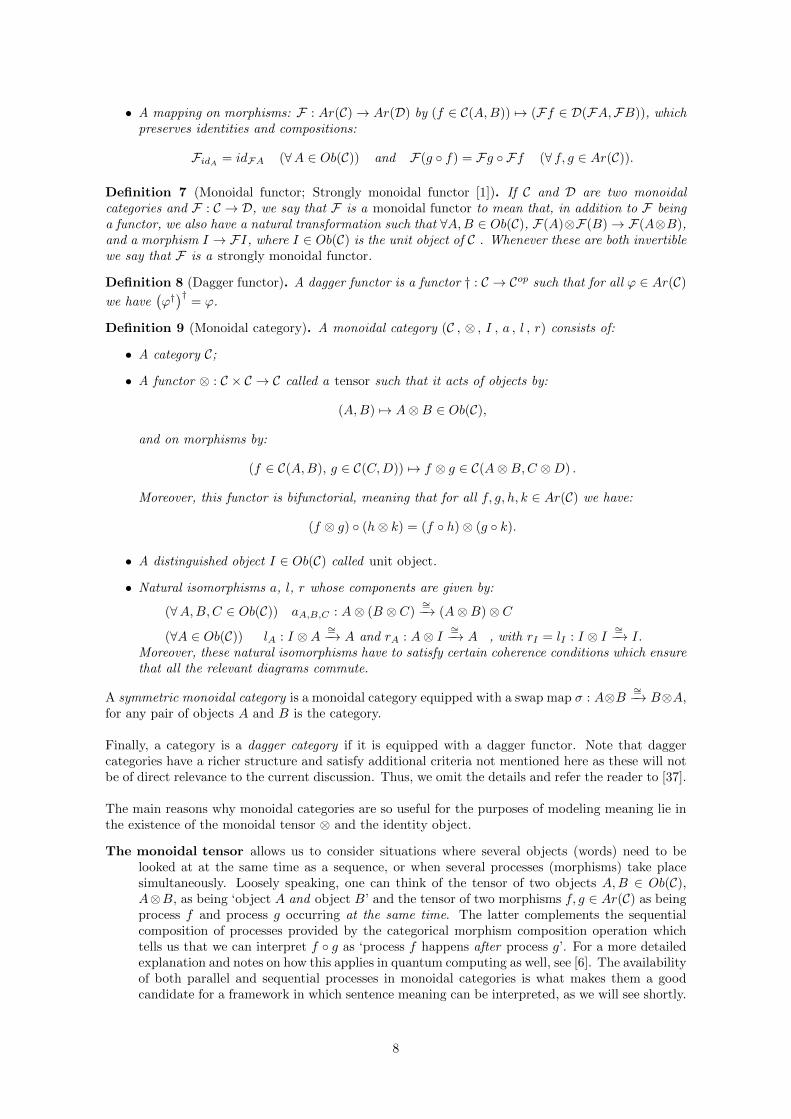
Definition 7 (Monoidal functor; Strongly monoidal functor [1]). If C and D are two monoidalcategories and F : C ! D, we say that F is a monoidal functor to mean that, in addition to F beinga functor, we also have a natural transformation such that 8A,B 2 Ob(C), F(A)⌦F(B) ! F(A⌦B),and a morphism I ! FI, where I 2 Ob(C) is the unit object of C . Whenever these are both invertiblewe say that F is a strongly monoidal functor.
Definition 8 (Dagger functor). A dagger functor is a functor † : C ! Cop such that for all ' 2 Ar(C)we have
�'†�† = '.
Definition 9 (Monoidal category). A monoidal category (C , ⌦ , I , a , l , r) consists of:
• A category C;
• A functor ⌦ : C ⇥ C ! C called a tensor such that it acts of objects by:
(A,B) 7! A⌦B 2 Ob(C),
and on morphisms by:
(f 2 C(A,B), g 2 C(C,D)) 7! f ⌦ g 2 C(A⌦B,C ⌦D) .
Moreover, this functor is bifunctorial, meaning that for all f, g, h, k 2 Ar(C) we have:
(f ⌦ g) � (h⌦ k) = (f � h)⌦ (g � k).
• A distinguished object I 2 Ob(C) called unit object.
• Natural isomorphisms a, l, r whose components are given by:
(8A,B,C 2 Ob(C)) aA,B,C : A⌦ (B ⌦ C)⇠=�! (A⌦B)⌦ C
(8A 2 Ob(C)) lA : I ⌦A⇠=�! A and rA : A⌦ I
⇠=�! A , with rI = lI : I ⌦ I
⇠=�! I.
Moreover, these natural isomorphisms have to satisfy certain coherence conditions which ensurethat all the relevant diagrams commute.
A symmetric monoidal category is a monoidal category equipped with a swap map � : A⌦B⇠=�! B⌦A,
for any pair of objects A and B is the category.
Finally, a category is a dagger category if it is equipped with a dagger functor. Note that daggercategories have a richer structure and satisfy additional criteria not mentioned here as these will notbe of direct relevance to the current discussion. Thus, we omit the details and refer the reader to [37].
The main reasons why monoidal categories are so useful for the purposes of modeling meaning lie inthe existence of the monoidal tensor ⌦ and the identity object.
The monoidal tensor allows us to consider situations where several objects (words) need to belooked at at the same time as a sequence, or when several processes (morphisms) take placesimultaneously. Loosely speaking, one can think of the tensor of two objects A,B 2 Ob(C),A⌦B, as being ‘object A and object B’ and the tensor of two morphisms f, g 2 Ar(C) as beingprocess f and process g occurring at the same time. The latter complements the sequentialcomposition of processes provided by the categorical morphism composition operation whichtells us that we can interpret f � g as ‘process f happens after process g’. For a more detailedexplanation and notes on how this applies in quantum computing as well, see [6]. The availabilityof both parallel and sequential processes in monoidal categories is what makes them a goodcandidate for a framework in which sentence meaning can be interpreted, as we will see shortly.
8

The identity element I 2 Ob(C) allows us to think down to the level of the elements of which theobjects of the category are built, while at the same time retaining the generality provided by thecategorical formalism. This is because the properties of the identity object imply the existenceof a bijective correspondence between the actual elements of A 2 Ob(C) and morphisms of thetype a : I ! A, where a 2 C(I, A). This correspondence will allow us to think of words as beinglinear maps in a vector space and at the same time its elements.
Graphical Calculus for monoidal categories
Another significant advantage of monoidal categories is that they are complete with respect to avery intuitive graphical calculus. By completeness we mean that any statement about the equalityof morphisms in a monoidal category can be derived from the categorical axioms if and only if thesame statement can be obtained via an admissible sequence of manipulations of diagrams expressiblein the monoidal graphical calculus.
The origins of this useful graphical language date back to Roger Penrose [31], who first proposedrepresenting morphisms (processes) as boxes and objects (input and output types) as wires. For moredetails about the origins and development of the graphical calculus, its applications in categoricalquantum computing, and a proof of the above statement, see [5, 38]. We will now only present themost basic diagrams and supplement these with other constructions as necessary later. The mainbuilding blocks of the diagrammatic calculus are boxes of various shapes and wires, which also giverise to the name string diagrams.
If A,B 2 Ob(C) and f 2 C(A,B) is a morphism thenwe represent it as a box with input wire labeled A andoutput wire labeled B. We adopt the convention herethat information flows from top to bottom.
f
A
B
For any A,B,C,D 2 Ob(C) and f 2 C(A,B), g 2C(C,D) the parallel morphism composition, i.e. the ten-sor of morphisms
f ⌦ g 2 C(A⌦ C,B ⌦D)
is depicted by simply placing the corresponding boxesnext to each other.
f
g
A
B
C
D
f
g
A
B
C
For any A,B,C 2 Ob(C) and f 2C(A,B), g 2 C(B,C) the sequential com-position
g � f 2 C(A,C)
is represented by simply stacking theboxes on top of each other, with the flowof information from one process of theother carried via the wire of their com-mon type B.
9

Note that if a morphism has several inputs and/or outputs then we represent these as di↵erent wiresinto/out of the appropriate morphism box. For example, f 2 C(A⌦B,C ⌦D) as a single morphismtakes the form
f
A B
C D
The identity object I 2 Ob(C) is depicted by an empty box and for each A 2 Ob(C) the identitymorphism 1A : A ! A takes the form of a single wire of type A.
Whenever we have a morphism with no inputs or out-puts, i.e. when the input or outputs are of type I, we de-pict these as up and down triangles respectively. Theseare normally denoted by ' : I ! A and ⇡ : A ! Iand are called states and e↵ects, following the quantumterminology.
⇡
A
A
[18] If A and B are two objects in our monoidal category then we call a morphism f : I ! A ⌦ Ba joint state of A and B. A joint state is said to be a product state or separable if it has the form
' : I ! I ⌦ If⌦g���! A⌦B, where f : I ! A and g : I ! B. Joint states which are not product states
are called entangled states. The diagram on the left hand side depicts a product state and the oneon the right is an entangled state.
A B A B
f
g '
Entangled states represent tensors A ⌦ B which cannot be decomposed into A and B as there issome kind of intrinsic interconnectedness between the two. For example, we could have an element
!�!a ⌦�!b 2 A ⌦ B which cannot be separated into ⇢�!a 2 A and �
�!b 2 B. This is very handy when
depicting functional words like verbs since in such cases we want to be able to represent the insep-arability of the constituents. This is essentially what allows us to put together a sentence in whichthe words have a way of interacting with each other, rather than simply existing next to one anotherin a string. This will become more clear when we define functional words in tensor spaces explicitlyand start performing calculations.
More complicated processes are depicted diagrammatically by combining these building blocks. Notethat the topology of the diagrams, i.e. the relative positions of the boxes and wires is immaterial asthe only thing of importance is how these are connected. For more on this refer to [5]. For example,the following two diagrams, and their corresponding morphisms, are in fact equal:
10

f
g
⇡
h
B
C
E
D
F
A A A
f
B
g
h
⇡
C
EA A A
F
D
(⇡ ⌦ h⌦ 1F ) � (g ⌦ 1D ⌦ ) � f (⇡ ⌦ 1A ⌦ 1A ⌦ 1A ⌦ 1F ) � (g ⌦ h⌦ 1F ) � (f ⌦ 1F ) �
2.2.3 Compact closed categories
Now we only need the morphisms for interpreting the grammatical reductions defined in the frameworkof the pregroup grammars. These are provided by compact closed categories.
Definition 10 (Compact closed category). A compact closed category C is a monoidal category inwhich for any object A 2 Ob(C) there exists a pair of objects Ar and Al also in Ob(C), called the rightand left adjoint of A, and corresponding structural morphisms "rA, "
lA. ⌘
rA, ⌘
lA given by:
A⌦Ar "rA�����! I Al ⌦A
"lA�����! I I
⌘rA�����! Ar ⌦A I
⌘lA���! A⌦Al
The first two of these are also known as cancellations and the second pair as generations. Thesesatisfy the following equations, known as the yanking equations:
(1A ⌦ "lA) � (⌘lA ⌦ 1A) = 1A
("rA ⌦ 1A) � (1A⌦ ⌘rA) = 1A
("lA ⌦ 1A) � (1Al ⌦ ⌘lA) = 1Al
(1Ar ⌦ "Ar ) � (⌘rA ⌦ 1Ar ) = 1Ar
Graphical calculus for compact closed categories
The structural morphisms are depicted as caps and cups in the languages of the graphical calculusaccompanying monoidal categories. We will use the following conventions:
Al A A Ar
A Al Ar A
cups
caps
"lA : Al ⌦A ! I "rA : A⌦Ar ! I
⌘lA : I ! A⌦Al ⌘rA : I ! Ar ⌦A
Graphical calculus for †-compact closed categories
It will be easier to adopt the convention of drawing morphisms as asymmetric boxes when they inhabita dagger compact closed category. Note that this convention will not be applied to states and e↵ectswhich will still be depicted as triangles. So, for a general morphism ' : A ! B we have:
11

A
B
'
Then we depict application of the † functor to ' as a reflection of the box along the horizontal axis,i.e '† : B ! A is depicted as:
B
A
'
Definition 11 (Name, Coname [18]). Let C be a †-compact closed category. We define the name andconame of a morphism ' 2 C (A,B) to be (respectively) the morphisms:
p'q : I ! A⇤ ⌦B
p'q = (idA⇤ ⌦ ') � ⌘A
'
A
⇤B
x'y : A⌦B⇤ ! I
x'y = "B � ('⌦ idB⇤)
'
A B
⇤
Definition 12 (Dual morphism [18]). Define the dual of a morphism ' : A ! B to be '⇤ : B⇤ ! A⇤,given by:
'
B
⇤
A
⇤
which is obtained via
12

'
⇤'
B
⇤
A
⇤A
⇤
B
⇤
A
⇤
A
B
B
⇤
'
= =yank
Finally, we define '⇤ =�'†�⇤ to be:
B
A
'
A
⇤
B
⇤
'
*
=
Note that applying † to the " and ⌘ maps has the e↵ect of reflecting them along the horizontal axis.
2.3 Uniting syntax and semantics via a compact closed cate-gory
We are finally in the position to describe the structures that we already defined as the containers forgrammar and meaning in the language of category theory.
2.3.1 Pregroup grammars as compact closed categories
A pregroup grammar G =⇣P , , · , 1 (·)r , (·)l⌘ is a compact closed category C = Preg:
• The objects are the elements of the underlying set P .
• The morphisms, denoted by ‘!’ or ‘’, correspond to the partial order between the elementsof P in the sense that there is a morphism between p, q 2 Ob(C) i↵ p q as elements of P .Note that if there exists a morphism between any pair of objects then it is necessarily unique.In other words, between any two objects of the category there is either one morphism or none.
• The existence of composite morphisms follows from the transitivity of the partial order of P :
(p q) ^ (q r) =) (p r) 8 p, q, r 2 P.
We can also express this by saying that ‘p ! q’ and ‘q ! r’ implies ‘p ! r’ for any p, q, r 2Ob(C).
• The existence of an identity morphism on any object p 2 Ob(C) follows from the reflexivity ofthe partial order:
p p 8 p 2 P.
We also write ‘p ! p’.
• The monoidal tensor ⌦ of C is the monoidal multiplication · : P ⇥ P �! P of G.- The tensor on objects p⌦ q (p, q 2 Ob(C)) is given by p·q, which we simply write as pq.
- The tensor on morphisms follows from the transitivity of the partial order on P and theorder-preserving property of the monoidal multiplication as follows:
[((p q) =) pr qr) ^ ((r s) =) qr qs)] =) pr qr qs =) pr qs.
13

• The left and right adjoints of p 2 Ob(C) are simply the left and right adjoints of the elementp 2 P , which exists by definition of G.
• The structure-preserving " and ⌘ maps are given by:
"l = pl·p ! 1 ⌘l = 1 ! p·pl"r = p·pr ! 1 ⌘r = 1 ! pr·p
Note that we may alternatively write ‘’ instead of ‘!’, e.g. "l = [pl·p 1]. One can easilyverify that these satisfy the compact closure axioms.
Let B = {n, s,�, j} be the set of basic grammatical types that we had before. We will denote byPregB the compact closed category corresponding to the pregroup grammar G used to model thegrammar and grammatical reductions of strings of words. As a compact closed category, PregB isaccompanied by a graphical calculus. This comes very handy as the graphical depictions of the " and⌘ maps greatly simplify grammatical reductions. To see this, consider the reduction of one of ourprevious examples done via a string diagram:
nJohn
nr
dislikess nl n nl
the postmodern
n
paintings
nr n nll slthat
n
Mary
nr s nl
buys
What this diagrams tells us is that the output type of the combined morphisms is simply s, as thisis the type of the only outgoing wire. Thus, the type of the sentence is s, as expected.
2.3.2 Finite dimensional Hilbert spaces as compact closed categories
The category in which we will model meaning is FHilb. Note that in the literature, meaning is oftenmodeled in the category of finite-dimensional (real) vector spaces and linear maps FVect. In prac-tice, which of these is used for the purposes of any of the applications mentioned in the present workmakes no di↵erence, as in either case we restrict our attention to real vector spaces and a very narrowset of morphisms. The advantage of working with FHilb is that it allows for more structure and isequipped with a canonical inner product that gives rise to adjoints. It is is a motivating example forthe class of dagger compact closed categories used in the CPM construction, which will be elaboratedon in the next chapter.
Let H be an arbitrary Hilbert space. Then H has an inner product h· | ·iH : H ⇥H ! C, which is:
• antilinear in the first argument: h�f + g |hiH = �hf | giH + � hg |hiH (� 2 C) ;
• linear in the second argument: hf |�g + hiH = �hf | giH + �hf |hiH ;
• conjugate-symmetric: hf | giH = hg | fiH ;
• positive semi-definite: hf | fiH � 0.
Note that when there is no ambiguity, we will simply write h· | ·i instead of h· | ·iH . The adjoint ofa liner maps is now defined via the canonical inner product.
Definition 13 (Adjoint of linear map). If V and W are Hilbert spaces and ' : V ! W is a linearmap between them then its adjoint is defined to be the unique linear map '† : W ! V such that8f 2 V and g 2 W , we have:
h'f | giW = hf |'†giV .
This defines a natural dagger functor on FHilb.
Definition 14 (Adjunctor functor). The adjunctor functor † : FHilb ! FHilbop is a functor whichpreserves objects and takes morphisms ' 2 Ar(FHilb) to their adjoints '† 2 Ar(FHilbop). This is
a dagger functor, i.e.�'†�† = '.
14

We can now formally define the category FHilb as the †-compact closed category with:
• Objects: finite dimensional Hilbert spaces over C.
• Morphisms : bounded C-linear maps.
• Morphism composition is provided by the closure under composition of C-linear maps.
• The unit object is the field itself.
• The monoidal tensor is the vector tensor product ⌦.
• The left V l and right V r adjoints of V 2 Ob(FHilb) are both given by the dual vector spaceV ⇤ of V . Note that by fixing a basis {�!ei }i for V we have that V ⇤ ⇠= V . Thus, from now on wewill adopt the convention of writing V to mean any of these: V , V r, V l, V ⇤.
• The structure-preserving maps " and ⌘ are given by:
"rV = "lV = "V : V ⌦ V �! R byX
ij
↵ij�!ei ⌦�!ej 7!
X
ij
↵ijh�!ei |�!ej i
⌘rV = ⌘lV = ⌘V : R �! V ⌦ V by 1 7!X
i
�!ei ⌦�!ei
where {�!ei }i is a basis for V and {1} is a basis for R. As we will only be interested in therestriction to real Hilbert spaces, this definition su�ces.
For the time being, the most important type of morphisms in FHilb for us will be the states. Recallthat a state is a morphism from the unit object to another object. In this case, it is a linear map ofthe form R ! V where V is a (real Hilbert) vector space. These are in a one-to-one correspondencewith elements of the space v 2 V , which can be established by considering the image of 1 2 R. Thus,we will write v : R ! V to mean the morphism that sends 1 7! v. This allows us the flexibility ofbeing able to think of states as morphisms and elements (of the vector space) at the same time. Moreconcretely, it allows us to consider individual words in a sentence as vectors even though in realitythey are linear maps. In other words, if we are working in some vector space V and want to depict a
word that lives in this space in the form of a vector���!word 2 V , we will draw:
V
word
Note that |vi|wi is often used as a shorthand for �!v ⌦�!w and we will use these notations interchange-ably.Note also that |vihw| ⇠= |vi|wi by writing the transpose of each row of the matrix |vihw| one after theother in a single column vector.
2.3.3 Meanings of sentences
Recall that we defined a way in which we can transition between two monoidal categories C and Dcalled a functor, and in particular we had a subclass of functors called strongly monoidal functors. Avery useful property of strongly monoidal functors applied to compact closed categories is that theypreserve the compact closure structure in the following sense:
F(Ar) = F(A)r and F(Al) = F(A)l 8A 2 Ob(C).
The transition between the category PregB of grammar and the category FHilb of word meaning isachieved via a strongly monoidal functor F : PregB �! FHilb. Note that it su�ces to consider theaction of this functor on the elements of the generating set B and the morphisms between elementsof this set. We have:
15

F : Ob(PregB) �! Ob(FHilb) by x 7!
8><
>:
N if x 2 {n,�, j}S if x := s
I = R or C if x := 1
Here N is taken to be the vector space containing the nouns and spanned by the appropriate basiscontext vectors and S is the vector space that is meant to contain the meanings of sentences. Notethat in practice we will sometimes take subspaces of N for the various nouns we consider, e.g. forobjects and subjects of sentences, and also that there is no fixed vector space that gets assigned to Sby default. We may have one or two-dimensional sentence space or even S = N⌦N depending on theproblem at hand. As these will depend on specific applications, we will define them accordingly when-ever necessary later in this thesis. A brief account of this is provided in the last section of this chapter.
F : Ar(PregB) �! Ar(FHilb) maps partial orders between elements of B to linearmaps between the appropriate vector spaces.
Some useful properties of the functor include:
• F(xr) = F(x) = F(xl) for any element x in the pregroup grammar. This follows from the factthat for finite dimensional vector spaces we have V ⇠= V ⇤ and hence F(V ⇤) = F(V ).
• F(Xrr) = F(x) = F(xll) for any x in the grammar. This follows from V ⇤⇤ ⇠= V , and thusF(V ⇤⇤) = F(V ).
• Functoriality tells us that if x = s1
. . . sn is any string, i.e. element, in the pregroup grammar,then F(x) = F(s
1
)⌦ . . .⌦ F(sn).
• Preservation of the compact closure maps " and ⌘.
For example, we have that:
F(nrsnl) = F(nr ⌦ s⌦ nl) = F(nr)⌦ F(s)⌦ F(nl)
= F(n)⌦ F(s)⌦ F(n)
= N ⌦ S ⌦N,
and nrsnl is the type of a transitive verb, so we conclude that the meanings of transitive verbs livein the tensor space N ⌦ S ⌦N . In other words, we may represent a transitive verb as:
verb =X
ijk
Cverbijk
�!ei ⌦�!sj ⌦�!ek ,
where {ei}i is a basis for N and {sj}j for S and the coe�cients Cverbijk come from the underlying field
R. Diagrammatically, a verb looks like this:
verb
N S N
Similarly, for adjectives we get F(nnl) = F(n ⌦ nl) = F(n) ⌦ F(nl) = N ⌦ N , and hence we canrepresent these as:
adjective =X
ij
Cadjij
�!ei ⌦�!ej .
Finally, we define the meaning of a string of words as follows. Suppose that we have a string of words(not necessarily a well-typed sentence) s = w
1
. . . wn and let the type of word wi be ti. These types,as well as the composite type of s, t
1
. . . tn, are objects in the category PregB. Now suppose thatwe have a type reduction t
1
. . . tnr��! x for some type x that cannot be reduced any further but
16

need not be a basic type. This reduction r is tensor and/or composition of structural morphisms ofthe category PregB and can therefore be translated into the corresponding morphisms in FHilb viathe strongly monoidal functor F . It is exactly this translation that allows us to make the transitionbetween grammar and meaning. More precisely, we define:
Definition 15. The from-the-meaning-of-words-to-meaning-of-sentences map, or simply meaningmap for a string of words s = w
1
. . . wn with grammatical reduction r is given by:
F(r)(�!w1
⌦ . . .⌦�!wn).
For example, consider the sentence Carnivorous animals eat meat. The word types are, in theorder in which they appear, nnl, n, nrsnl, n. The types reduction r is given by:
(nnl)n(nrsnl)n = n(nln)nrs(nln)1
n
⌦"ln
⌦1
n
⌦1
s
⌦"ln������������! (nnr)s
"rn
⌦1
s����! s,
sor = ("rn ⌦ 1s) � (1n ⌦ "ln ⌦ 1n ⌦ 1s ⌦ "ln).
Hence, the meaning of the sentence is given by:
F(("rn ⌦ 1s) � (1n ⌦ "ln ⌦ 1n ⌦ 1s ⌦ "ln))(��������!carnivorous⌦
�����!animals⌦�!
eat⌦���!meat)
= ("N ⌦ 1S) � (1N ⌦ "N ⌦ 1N ⌦ 1S ⌦ "N )(��������!carnivorous⌦
�����!animals⌦�!
eat⌦���!meat).
Carnivorous animals eat meat
N N N N S N N
carnivorous animals eat meat
n nl n nr s nl n
From the diagram we can simply read o↵ the meaning map, which is:
' = ("N ⌦ 1S) � (1N ⌦ "N ⌦ 1N ⌦ 1S ⌦ "N ).
Suppose that the individual words in the sentence are given by:
carnivorous =X
i
Ccarnii
�!ni ⌦�!ni�����!animals =
X
k
↵k�!nk
���!meat =
X
j
�j�!nj eat =
X
lrt
Ceatlrt
�!nl ⌦ sr ⌦�!nt
Then we obtain the meaning of the sentence as:
'⇣carnivorous⌦
�����!animals⌦ eat⌦���!
meat⌘.
= '
0
@X
i
Ccarnii
�!ni ⌦�!ni ⌦X
k
↵k�!nk ⌦
X
lrt
Ceatlrt
�!nl ⌦ sr ⌦�!nt ⌦X
j
�j�!nj
1
A
= ("N ⌦ 1S)
0
@X
ijklrt
Ccarnii ↵k C
eatlrt �j h�!ni |�!nkih�!nt|�!nji�!ni ⌦�!nl ⌦ sr
1
A
= ("N ⌦ 1S)
0
@X
ijlr
Ccarnii ↵i C
eatlrj �j
�!ni ⌦�!nl ⌦ sr
1
A
=X
ijrl
Ccarnii ↵i C
eatlrj �j h�!ni |�!nli sr
=X
ijr
Ccarnii ↵i C
eatirj �j sr.
17

2.4 Relative clauses via Frobenius algebras
We introduce very briefly the additional structure on top of compact closed categories developedin [34,35], which allows for modeling sentences and phrases containing relative pronouns that, which,who, whose and the possessive whose. This additional structure is provided by the so-called Frobeniusalgebras, first developed by F. G. Frobenius.
Definition 16 (Frobenius algebra [34]). Let C be a symmetric monoidal category and A 2 Ob(C). AFrobenius algebra A over C is a tuple (A, �, ◆, ⇣, µ) where:
• (A, µ : A⌦A ! A, ⇣ : I ! A) is an internal monoid;
• (A, � : A ! A⌦A, ◆ : A ! I) is an internal comonoid.
These together satisfy the Frobenius condition:
(µ⌦ 1A) � (1A ⌦�) = � � µ = (1A ⌦ µ) � (�⌦ 1A) .
For a definition of monoid and comonoid see, e.g. [3], and for more on Frobenius algebras refer to [20].For our purposes we will only need to consider Frobenius algebras over FHilb.
Let V 2 Ob(FHilb) be a finite-dimensional (real) Hilbert space with basis {�!ei }i. We define aFrobenius algebra over it by:
µ :V ⌦ V ! V ⇣ : I ! V � : V ! V ⌦ V ◆ : V ! I
�!ei ⌦�!ej 7! �ij�!ei 1 7!
X
i
�!ei �!ei 7! �!ei ⌦�!ei �!ei 7! 1
The intuition behind using these to model language structures can be summarized according to [35] as:
The comonoid’s comultiplication � is often referred to as copying. It has the e↵ect of produc-ing a diagonal matrix out of a vector, i.e. �(�!v ) is the diagonal matrix in V ⌦ V whose diagonalentries are the coe�cients of �!v . Copying enables the transfer of information contained in a singlevector (or the vector space it belongs to) to two others. For example, by copying the information con-tained in a noun vector we can feed the two copies into a relative pronoun and a verb at the same time.
The monoid’s multiplication µ is referred to as uncopying. It extracts the diagonal entries of amatrix and produces a vector with these as coe�cients. Uncopying allows us to merge the informationcoming from two di↵erent sources. This can be used in cases where we need to put back together theinformation produced after processing di↵erent parts of a sentence containing a relative clause into asingle output.
The unit ◆ lets us discard information. For example, a relative pronoun takes as input from theverb a wire of type S corresponding to sentence type s, but does not produce an output of the sametype (as relative clauses output noun-types) and has to discard it.
Diagrams for Frobenius algebra morphisms.
µ : A⌦A ! A ⇣ : I ! A � : A ! A⌦A ◆ : A ! I
The Frobenius condition is depicted as:
18

= =
Applications of the Frobenius maps to vector are depicted as the composition of the Frobenius mapwith the corresponding state:
µ (�!v ⌦�!w ) � (�!v ) ◆ (�!v )
V W V
V
vvwv
VV V
where v : I ! V and w : I ! W .
2.4.1 Relative pronouns via Frobenius algebras
Recall that the grammatical type of the subject relative pronouns who, that and which is nrnsln andthat of the object relative pronouns whom, that and which is nrnnllsl. The grammatical reductionsof relative clauses are established as follows.
n nr n sl n nr s nl n
subject relative pronoun verb object
subject relative clause
n nr n nll sl n nr s nl
object relative pronoun subject verb
object relative clause
Note that the output in either case is of type n, as expected from a well-typed relative clause.Applying the functor F : PergB ! FHilb to the types of the relative clauses gives us the tensorspaces in which their meanings live.
F�nrnsln
�= N ⌦N ⌦ S ⌦N
F�nrnnllsl
�= N ⌦N ⌦N ⌦ S
According to [34], these are functional words explicitly given in FHilb as:
19

N N S N N N N S
subject object
(1N ⌦ µN ⌦ ⇣S ⌦ 1N ) � (⌘N ⌦ ⌘N ) (1N ⌦ µN ⌦ 1N ⌦ ⇣S) � (⌘N ⌦ ⌘N )
Then the diagrammatic representations for subject and object relative clauses become:
subject relative clause
N N N S N N S N N
subject relative pronoun verb object
object relative clause
N N N SN N SN N
subjectrelative pronoun verbobject
These reduce to:
subject relative clause object relative clause
N N S N N N N NS N
subject verb object subject verb object
(µN ⌦ ◆S ⌦ "N )⇣��!subj ⌦ verb⌦
�!obj⌘
("N ⌦ ◆S ⌦ µN )⇣��!subj ⌦ verb⌦
�!obj⌘
Note that these can now be used in more complicated structures, such as nested relative clauses orpositive transitive sentences containing various subject or object relative clauses. For concrete exam-ples, see [34]. We will use instances of this construction with in the framework of the CPM(FHilb)in the final chapter.
In their paper [35], Sadrzadeh, Clark and Coecke apply Frobenius algebras in a similar fashion inorder to model meanings of possessive subject and object relative clauses, i.e. structures of the formpossessor whose subject verb object and possessor whose object subject verb. These arenot discussed here.
20

2.5 Concrete vector spaces for nouns and sentences
So far we haven’t said much about how the vector spaces N and S are chosen and how the output ofthe meaning map can be interpreted so as to make the categorical compositional model of [7] trulydistributional and practically applicable. A detailed discussion of the various options that have beenutilized so far and experimental support is not necessary here, but the reader is referred to [12–14,36].We will simply outline two main approaches that can be adopted and which are used later on in thisthesis in computations of examples.
We will introduce a running example that will help illustrate the di↵erent approaches to choosingN and S and show the kind of results we obtain in practice. This will be a simple positive definitesentence, but a very similar approach can be adopted when representing adjective-noun phrases andmore complicated structures involving various phrases and even adverbs [14]. The example will beDetectives pursue criminals. Without specifying the common noun space N and sentence spaceS, we define the individual word vectors as:
�������!detectives =
X
i
↵i�!ni
�������!criminals =
X
j
�j�!nj
����!pursue =X
prt
Cprt�!np ⌦�!sr ⌦�!nt.
The meaning of the sentence is given by
N N S N N
Detectives pursue criminals
("N ⌦ 1S ⌦ "N )⇣�������!detectives⌦����!pursue⌦
�������!criminals
⌘
= ("N ⌦ 1S ⌦ "N )
0
@X
i
↵i�!ni ⌦
X
prt
Cprt�!np ⌦�!sr ⌦�!nt ⌦
X
j
�j�!nj
1
A
=X
iprtj
↵i Cprt �j hni |npi sr hnt |nji
=X
irj
↵i Cirj �j sr
(2.1)
2.5.1 Truth-theoretic meaning
In [7], the compositional categorical model of meaning introduced in the paper is applied in a truth-theoretic setting, in which we assume that the noun vectors are all (standard) orthonormal basisvectors in a vector space N , chosen to be the span of a suitable set of vectors which can be as smallas simply the set of those basis vectors that represent the nouns under consideration. The sentencespace S is taken to be one- or two-dimensional and truth-theoretic. In the one-dimensional case, i.e.when S = Span{�!1 } we can take the basis vector
�!1 to stand for true and
�!0 for false. Alternatively,
we can work with S = Span{|0i, |1i}, in which case |0i =✓10
◆stands for true and |1i =
✓01
◆for false.
In our example, we can take N to be the two dimensional vector space spanned by:
�!n1
=
✓10
◆=
�������!detectives and �!n
2
=
✓01
◆=
�������!criminals,
and S to be the one-dimensional vector space with Cirjsr =
(�!1 if �!ni pursues �!nj�!0 o.w.
.
Then (2.1) returns�!1 whenever it is true that detectives pursue criminals (according to our sources)
21

and�!0 otherwise. The same outcome can be achieved if we take S to be 2-dimensional. Also,
note that if we increase the size of the noun space by, e.g., including basis vectors for all possible
detectives and criminals and representing the vectors�������!detectives and
�������!criminals as sums of these, the
above calculation will result in a sum of�!1 ’s and
�!0 ’s, where there will be as many
�!1 ’s in this sum
as there are detective-criminal pairs of people in the relationship of the latter being pursued by theformer. This can be generalised in other ways, such as by adding weights to the vectors that go intothe sums corresponding to the nouns, or even by representing the verb as a sum of other actions, e.g.:
����!pursue =1
2
��������!investigate+
1
2
���!chase.
For worked examples of this form see [7].This framework is useful for a limited number of applications and for proof of concept examples,but is otherwise essentially no di↵erent from the model-theoretic view on semantics. For a trulydistributional perspective, we need to extract the word meanings from a corpus. Moreover, in thecase where the output of the meaning map is of type s, taking S to be truth-theoretic does not tellus anything about the features of the individual words that comprise the sentence and how theseinteract with each other to produce the output. As such, it is not a very useful space to work withwhen considering practical tasks, or even for sentence comparisons.
2.5.2 A more distributional approach to word meaning and a new sentencespace
The idea developed in [14] is to take N to be a structured vector space like in other applications of thedistributional models framework. The basis vectors of this space can be taken to be a set of propertiesor salient features of the nouns, depending on the application we are interested in. In the case ofapplications in the area of cognitive linguistics, such as [25], these basis vectors can be taken to bethe salient features of the nouns that do not necessarily have to be extracted from a corpus, but canbe obtained from target groups in controlled experiments. We will see an example of this in Chapter 4.
In cases where we are interested in practical linguistic applications (definitions, ambiguity, informationretrieval, sentence comparisons, etc.) and working with a corpus, these vectors can be obtaineddirectly from the corpus via statistical (co-occurrence) methods. In this thesis, we will use theapproach of [14] for the purposes of toy examples whenever this is more suitable than a simple truth-theoretic model. We will illustrate how this approach works by means of an example. Suppose thefollowing are basis vectors for N : arg-strong, subj-build, obj-clean. Then if we want to represent anoun �!n with respect to these basis vectors, it will have entires that express how many times in thecorpus this noun has appeared as the argument of the adjective strong, the subject of the verb buildand the object of the verb clean. The sentence space can be taken to be S = N ⌦ N , so that thebasis vectors for S are of the form �!ni ⌦ �!nj , where
�!ni ,�!nj are basis elements of N . Verbs are then
represented as: ��!verb =
X
ij
Cverbij
�!ni ⌦ (�!ni ⌦�!nj)⌦�!nj .
The intuition behind this is that it allows us to output a meaning of the sentence in the form of amatrix that contains all the information that we get from modifying the features of the noun objectand subject via the verb. The weights Cverb
ij are built by counting the number of times that a wordwhich is a possessor of property ni is the subject of this verb and a word that has property nj is its ob-ject, i.e. how many times we have in the corpus (something which is ni) verb (something which is nj).
For example, suppose that we have (standard) basis vectors {n1
, . . . n5
} representing, in this order,arg-cunning, arg-righteous, arg-nasty, arg-meticulous, obj-kill and in our imaginary corpus the worddetective has appeared 4 times as the argument of cunning, 5 times as the argument of righteous, 3times as the argument of meticulous and once as the object of kill. Suppose that the word criminalhas appeared twice as the argument of cunning and meticulous, 3 times as the argument of nasty.
22

Then the vectors for the two words are given by:
������!detective =
0
BBBB@
45031
1
CCCCA,
������!criminal =
0
BBBB@
20320
1
CCCCA,
and the meaning of the sentences can be computed accordingly.
23
Chapter 3
The CPM construction and densitymatrix formalism
The model of meaning of [7] summarised in the previous chapter has been applied successfully to anumber of tasks [11–14, 25, 36]. However, restricting our attention to vectors as means of capturingword meaning also has limitations, which prevent us from making good use of it for some more in-volved applications that necessitate for the relationships between words and between concepts andtheir salient features to be taken into account. For this reason, some of the more recent work in thefield [2, 32, 33] has involved a shift of focus from vectors to density matrices to represent semantics.This approach has already proved to be promising for disambiguation [33] and in the modeling tohyponymy [2] and has given rise to many opportunities for further research.
Density matrices are used in quantum mechanics to represent uncertainty about the state of a phys-ical system. Not only do they possess richer structure than vectors, but they are also equippedwith mathematical properties that allow for the introduction of various symmetric and asymmetricmeasures of similarity and inclusion. In contrast, vectors can only be compared to each other viasymmetric measures, such as the cosine.
The mathematical framework in which density matrices occupy the same position as that of vectorswith respect to the †-compact closed category FHilb is the category CPM(FHilb), built on topof FHilb. Thus, in this chapter we will first introduce the CPM construction in the context of itsapplications to distributional models of meaning, following closely [33], and then shift our attentionto CPM(FHilb) and density matrices specifically.
3.1 The doubling construction and CPM
3.1.1 The doubling construction on †-compact closed categories
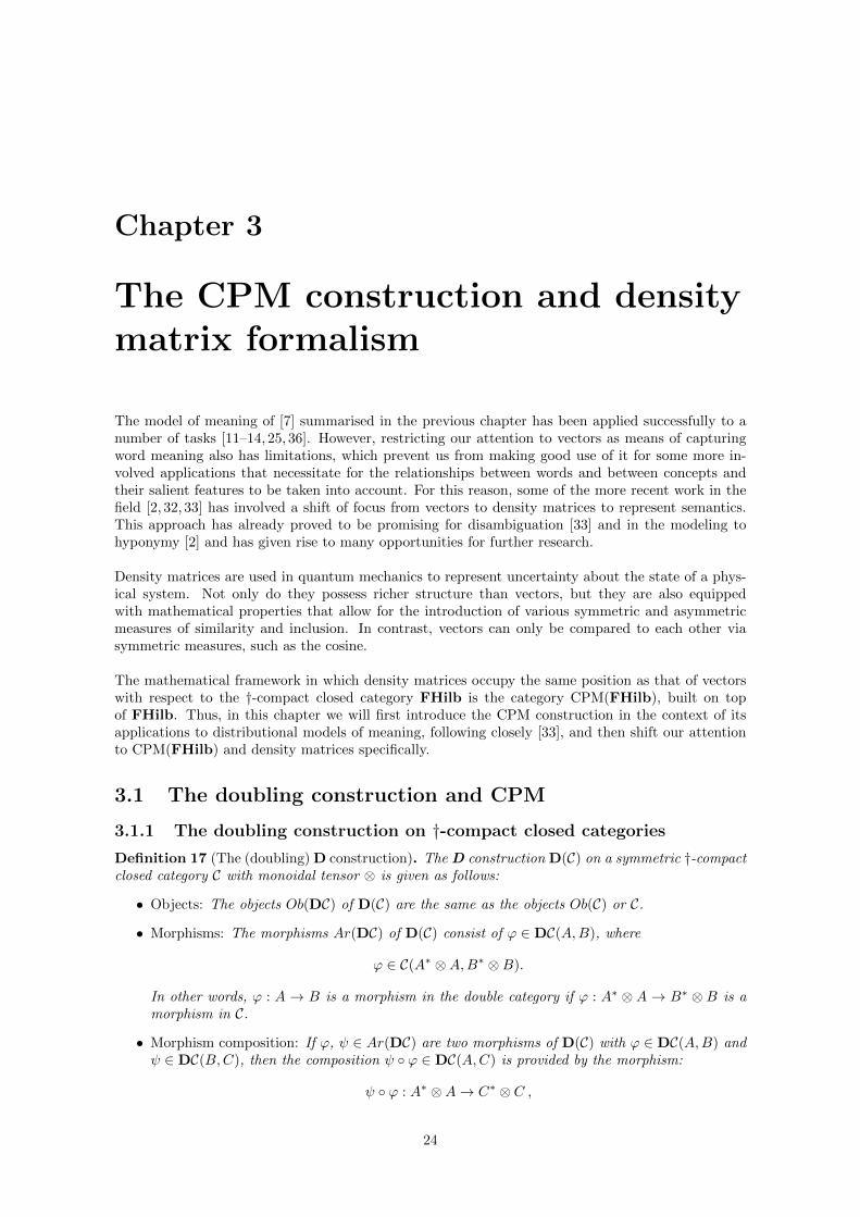
Definition 17 (The (doubling)D construction). The D construction D(C) on a symmetric †-compactclosed category C with monoidal tensor ⌦ is given as follows:
• Objects: The objects Ob(DC) of D(C) are the same as the objects Ob(C) or C.
• Morphisms: The morphisms Ar(DC) of D(C) consist of ' 2 DC(A,B), where
' 2 C(A⇤ ⌦A,B⇤ ⌦B).
In other words, ' : A ! B is a morphism in the double category if ' : A⇤ ⌦ A ! B⇤ ⌦ B is amorphism in C.
• Morphism composition: If ', 2 Ar(DC) are two morphisms of D(C) with ' 2 DC(A,B) and 2 DC(B,C), then the composition � ' 2 DC(A,C) is provided by the morphism:
� ' : A⇤ ⌦A ! C⇤ ⌦ C ,
24

whose existence follows from the composition of ' : A⇤⌦A ! B⇤⌦B and : B⇤⌦B ! C⇤⌦Cin C.
• Monoidal tensor: The monoidal tensor of D(C) is given by ⌦D : D(C) ! D(C), which acts
- on objects A,B 2 Ob(DC) as A⌦D B = A⌦B ;
- on morphisms ' 2 DC(A,B), 2 DC(C,D) :
'⌦D : A⇤ ⌦A⌦ C⇤ ⌦ C'⌦ ���! B⇤ ⌦B ⌦D⇤ ⌦D
Note that the existence of the swap map � : A⌦B⇠=�! B ⌦A in C implies that:
A⇤ ⌦A⌦ C⇤ ⌦ C ⇠= A⇤ ⌦ C⇤ ⌦ C ⌦A and B⇤ ⌦B ⌦D⇤ ⌦D ⇠= B⇤ ⌦D⇤ ⌦D ⌦B,
so we take:'⌦D : A⇤ ⌦ C⇤ ⌦ C ⌦A
'⌦ ���! B⇤ ⌦D⇤ ⌦D ⌦B.
Graphical calculus in DC
Our convention will be to represent the boxes and wires of D(C) with thicker lines so as to distinguishbetween the structures D(C) and C. This is done because the transfer from the latter category to theformer essentially means doubling of the wires. Thus, for example, the map ' 2 DC(A,B) is depictedas the LHS part of the diagram below, while its corresponding counterpart in C, ' : A⇤⌦A ! B⇤⌦B,as the RHS:
A
B
A
⇤A
B
⇤B
=
CD(C)
' '
The tensor of two morphisms ' and is depicted as:
'
B
⇤
A
⇤
D
⇤
C
⇤
B
A
D
C
'
7!
D(C) is also a †-compact closed category [37]. It inherits this structure from C via a strict monoidalfunctor E : C ! D(C) given by:
E :Ob(C) ! Ob(DC) E : Ar(C) ! Ar(DC)E ::A 7! A E :: f 7! f⇤ ⌦ f
and, inductively, E('⌦ ) = E(')⌦D E( ).
25

There is a bijective correspondence between the states of D(C) i.e. morphisms ' : I ! A⇤ ⌦ A of Cand the positive operators on A, i.e. morphisms : A ! A of C, established via the map that sendseach operator to its name:
f : C(A,A) ! C(I, A⇤ ⌦A)
' 7! p'q = (idA⇤ ⌦ ') � ⌘A
These states will be of central importance once we start working in the category CPM(FHilb). Recallthat the name of the operator ' : I ! A⇤ ⌦B, p'q is depicted (in C) as follows:
'
A
⇤B
3.1.2 The subcategory CPM(C) of D(C)Before we define the CMP(C) subcategory of D(C) we need the notion of a completely positive map.Completely positive maps arise naturally in the context of density matrices as they are essentiallydensity matrix-preserving maps. This concept will be made more precise later, but for now we givea general definition of completely positive maps that works in any †-compact closed category. Thedefinition below is due to Selinger [37].
Definition 18 (Completely positive morphism [33]). Let ' 2 DC(A,B) be a morphism of D(C), i.e.' : A⇤ ⌦A ! B⇤ ⌦B. We say that ' is a completely positive morphism if there exists C 2 Ob(DC)and k 2 C(C ⌦A,B), such that ' can be embedded in C by:
' 7! (k⇤ ⌦ k) � (1A⇤ ⌦ ⌘C ⌦ 1A) .
B
⇤B
A
⇤A
k k
CA
B
' 7!
C
⇤
Note that this implies that states in CPM(C) can be represented as:
'
k k
A A
⇤A
7!
and we can recover the original definition from above via:
A
⇤
'
k k
A
A
⇤A
=
k
A
k =
A
⇤
26

The second equality follows from the standard definition of positive operator, which tells us that' being positive means that we can express it as ' = k � k†. The LHS diagram will be the one usedin applications.
This representation implies that if f and g are two completely positive morphisms then the followingare also completely positive:
f � g , f ⌦ g , f⇤ ⌦ f = E(f). (3.1)
This essentially tells that any morphism in the category D(C) that can be obtained via a combinationof tensors and compositions of other completely positive morphisms is also completely positive. Thus,we have closure under � and ⌦ of completely positive morphisms in D(C), and hence can define thefollowing subcategory.
Definition 19 (CPM(C)). If C is a †-compact closed category then CPM(C) is the subcategory ofD(C) which has the same objects as C and its morphisms are the completely positive morphisms ofD(C).
Let I be the embedding of CPM(C) into D(C). Then there exists (by (3.1)) a strictly monoidal functorE : C ! CPM(C) such that E = IE.
The compact closure and Frobenius maps in CPM(C)
In the category CPM(C) the compact closure maps " and ⌘ are given by E(") and E(⌘), and similarlythe Frobenius algebra maps ◆, ⇣, µ and � are given my E(◆), E(⇣), E(µ) and E(�). Note thatwhenever there is no ambiguity as to which category we are working in, we will adopt the conventionof writing ", ⌘, µ, �, ◆ and ⇣ to mean the corresponding morphism in C or in CPM(C). Also, in thiscontext we are normally only interested in left adjoints, so we will write for each A 2 Ob(DC) :
"lA = " : A⇤ ⌦A ! I ⌘lA = ⌘⇤ : I ! A⌦A⇤
Later on, when working with real Hilbert spaces, it will not matter which map we mean, as the leftand right vector space adjoints are both isomorphic to the space itself.
Diagrammatic Calculus for CPM(C)
We will mainly be interested here in how the structure-preserving maps combine with the states ofthe category, so a brief discussion about this is in place. First of all, note that the diagrams for all ofthe structural morphisms and Frobenius maps are simply obtained from their original counterpartsby doubling the wires. For example, for the "-map in the CPM category, we get:
CPM(C) C
However, applying the map to the tensor of two states in CPM results in some swaps in the outputwires that occur because of the way that the tensor of morphisms is defined in CPM (see diagramabove). It will be more convenient for us to represent this in an alternative, but equivalent fashion,whereby we can treat, for example, the "-morphism as being:
CPM(C) C
To see how this works, consider the following diagram, in which on the LHS we have the diagrammaticrepresentation of " ('⌦ ) in CPM(C), in the middle we have the corresponding diagram in C andon the RHS - the equivalent representation that will be used in applications.
27

"
'⌦CPM
' '
' '
'
CPM(C) C
7! =
Thus, we can summarise these morphisms in CPM(C) via the following diagrams:
A
⇤A A
⇤A
⇤A A
A A
⇤A A
⇤A
⇤
E(") = "⇤ ⌦ "
" : A⇤ ⌦ A
⇤ ⌦ A⌦ A ! I
CPM(C) C
E(⌘) = ⌘⇤ ⌦ ⌘ ⌘ : I ! A⌦ A⌦ A
⇤ ⌦ A
⇤
CPM(C) C
" : (�!ei ⌦�!ej )⌦ (�!ek ⌦�!el ) 7! h�!ei |�!eki h�!ej |�!el i ⌘ : 1 7!X
ij
�!ei ⌦�!ej ⌦�!ei ⌦�!ej
A
⇤
A A
⇤A
⇤A A
AA
A A
⇤
A
⇤A
⇤
E(µ) = µ⇤ ⌦ µ µ : A⇤ ⌦ A⌦ A
⇤ ⌦ A ! A
⇤ ⌦ A
E(�) = �⇤ ⌦� � : A⇤ ⌦A ! A⇤ ⌦A⌦A⇤ ⌦A
A
A
AA A
A
µ : (�!ei ⌦�!ej )⌦ (�!ek ⌦�!el ) 7! h�!ei |�!eki h�!ej |�!el i(�!ei ⌦�!ej ) � : (�!ei ⌦�!ej ) 7! �!ei ⌦�!ej ⌦�!ei ⌦�!ej
A
⇤AA
A
⇤
E(◆) = ◆⇤ ⌦ ◆
◆ : I ! A
⇤ ⌦ A
E(⇣) = ⇣⇤ ⌦ ⇣ ⇣ : A⇤ ⌦A ! I
AA
◆ : (�!ei ⌦�!ej ) 7! 1 ⇣ : 1 7!X
i
�!e1
⌦�!ei
3.1.3 Sentence meaning in the category CPM(C)The CPM construction allows us to consider a number of new candidate categories in place of FHilbfor storing word meanings. As already mentioned, this thesis will only make use of CPM(FHilb),but since it is possible to work in other categories, such as CPM(Rel), we first define our sentencemeaning map in a more general setting where we do not explicitly specify the category that we wishto use, but rather work with a general †-compact closed category C and assume that our words existas states in the category CPM(C).
We now have all the necessary ingredients to define a new from-the-meaning-of-words-to-the-meaning-of-sentences map, or meaning map, that will allow us to transfer the grammatical structure of asentence to a category containing its words’ semantics, which is some CPM(C). Recall that in the
28

vector space model of distributional models of meaning the transition between syntax and semanticswas achieved via a strongly monoidal functor F : PregB ! FHilb. It turns out that we can similarlydefine a strongly monoidal functor S : PregB ! CPM(C). We define this functor to be S = EQ,where Q is the strongly monoidal functor Q : PregB ! C, of which F : PregB ! FHilb is a specialcase. The morphisms involved can be summarised via the following diagram:
CPM(C)
CPregB
D(C)
EQE
E
I
Q
Since Q is a strongly monoidal functor and E is strictly monoidal, we get that S is strongly monoidal,as required. We can now define the meaning map that makes use of CPM(C) as follows.
Fix a †-compact closed category C and its corresponding CPM construction CPM(C) with unitobject I. With the same notation as above we have:
Definition 20. Let s = w1
. . . wn be a string of words and let ti be the grammatical type of word wi inPregB. Suppose that the type reduction of s is given by t
1
. . . tnr��! x for some x 2 Ob(PregB). Let
⇢(wi) be the meaning of word wi in CPM(C), i.e. a state of the form I ! S(ti). Then the meaningof s is given by:
S(r) (⇢(w1
)⌦CPM . . .⌦CPM ⇢(wn)) . (3.2)
3.2 Modeling word and sentence meaning in CPM(FHilb)
From now on, we will only be working with the category CPM(FHilb) that is built out of the alreadyfamiliar category of finite dimensional Hilbert spaces and linear maps.
3.2.1 Density matrices as states in CPM(FHilb)
Recall that a state in a category C is a morphism of the form : I ! A for a vector space A, andthat the states in FHilb are in a one-to-one correspondence with the elements of the vector space inquestion.
Definition 21. A pure state on a vector space V is an operator V ! V which is of the form ' �'†,where ' : I ! V is a state and '† � ' = idI .
In quantum computing pure states represent the possible states in which a physical system can be.However, it is often the case that an observer does not have information about the exact state inwhich the system is, but rather only knows the probabilities attached to several possible states. Thiscan be mathematically expressed as a convex sum of pure states and we will call this a mixed state.More precisely, we use density matrices.
Suppose that a system can exist in state |⇢ii with probability pi, for some collection of state-probabilitypairs {|⇢ii, pi}. Then the density matrix or density operator corresponding to this system is givenby:
⇢ =X
i
pi |⇢iih⇢i|,
whereP
i pi = 1. Each of the |⇢iih⇢i| is a pure state.To see how these operators fit into our categorical framework, consider the following definition.
Definition 22 (Positive matrix [18]). We call a matrix a positive matrix if it is the name of apositive morphism ⇢ : V ! V , i.e. a morphism p⇢q : I ! V ⇤⌦V . The morphism ⇢ is called a mixedstate. Recall that these can be expressed diagrammatically as:
29

⇢
p⇢
p⇢
p⇢
p⇢= =
Thus, a density matrix, which is a positive matrix with trace 1, is exactly a state in CPM(FHilb)– the category which has as objects finite-dimensional Hilbert spaces and as morphisms completelypositive maps. Note that completely positive maps in this context means morphisms that take densitymatrices to density matrices and preserve their structure. All the formalism from the previous sectioncarries over to the category CPM(FHilb). Just as before, we will only be using real-valued vectorspaces and hence we will be able to assume that for all meaning spaces involved we have V ⇤ ⇠= V .
3.2.2 Using density matrices to model word meanings
How can density matrices be used to capture word meaning and what do we gain by doing this, asopposed to sticking to vector-based representations?
One use of density matrices that mirrors their role in quantum computing is in representing wordsas probabilistic mixtures of their possible ambiguous meanings. For example, in [33], the ambiguousnoun queen has the density matrix representation:
pqueenq = |ElisabethihElisabeth|+ |bandihband|+ |chessihchess|,
where Elisabeth, chess and band are assumed to be all the possible meanings of the word queen and,furthermore, these are assumed to be themselves pure states, i.e. they have unambiguous meanings.The idea behind using this kind of representation is that once the ambiguous word is put in a sentence,the functional words in this sentence interact with it in a similar way to how an observation a↵ects aphysical system. This allows for a single meaning to emerge out of the collection of possible meaningsand for this meaning to connect with the rest of the sentence and produce the relevant output, i.e.sentence meaning.
Another possible use of density matrices is in representing collective nouns as sums of their parts.For example, we could have that:
ppetq =X
i
pi ppetiq,
where ppetiq = |petiihpeti| is the pure state corresponding to the ith pet (e.g. pcatq, pdogq, etc).The advantage of doing this is that it lets us compare the collective nouns with their parts and seeconnections and di↵erences between them that are not immediately obvious when using vectors. Also,it allows for the introduction of various asymmetric measures which facilitate the comparison andordering of concepts and their components. Note that the same idea can be used for representingverbs or, indeed, any functional word in CPM(FHilb).
To see how these density matrices are formed in practice and how the morphisms work in theCPM(FHilb) category to form meaning maps and produce the meanings of sentences, consider thefollowing example, where for simplicity all the nouns are assumed to be pure states.
Example
Let the noun space be given by a real Hilbert space N with basis vectors given by {|nii}i, where for
some i, |nii =���!Clara and for some j, |nji =
��!beer. Let the sentence space be some unspecified S with
basis {|sii}i. Then the density matrices for the nouns Clara and beer are given by:
pClaraq = |niihni| and pbeerq = |njihnj |.
30

Suppose the verb��!like 2 N ⌦S⌦N is given by
��!like =
Prtv Crtv |nri|nti|nvi. Then its corresponding
density matrix in CPM(FHilb) is given by:
plikeq =
X
rtv
Crtv |nri|nti|nvi!
X
klu
Cklu|nki|nli|nui!T
=X
rtvklu
Crtv Cklu |nrihnk|⌦ |ntihnl|⌦ |nvihnu|
The meaning map is simply ("N ⌦ 1S ⌦ "N ) applied to (pClaraq⌦ plikeq⌦ pbeerq), as per the dia-gram below:
N N N N
Clara likes beer
N N N S N N S N N N
⇢(Clara likes beer) = ("N ⌦ 1S ⌦ "N ) (pClaraq⌦ plikeq⌦ pbeerq)
= ("N ⌦ 1S ⌦ "N )
|niihni| ⌦
X
klurtv
CrtvCklu |nrihnk|⌦ |stihsl|⌦ |nvihnu| ⌦ |njihnj |!
=X
klurtv
CrtvCklu hni |nri hni |nki (|stihsl|) hnv |nji hnu |nji
=X
ijtl
Citj Cilj |stihsl|
31

Chapter 4
Applications of distributionalcompositional models to cognitivelinguistics phenomena
In this chapter we consider applications of the DisCoCat model of meaning to two cognitive linguisticsphenomena, both of which possess some sort of asymmetry.
The so-called Pet Fish phenomenon is a classic example of overextension with respect to conceptcombination. We first give an overview of the recent work by Lewis and Coecke [25], who modeledthis example in the original setting, in which words are represented by vectors. We then go on toconsider the same in the new framework of CPM(FHilb).
The phenomenon of asymmetry in similarity judgments is examined in the classic experiments by A.Tversky [40], in which the perceived similarity of a more prominent country to a similar, but lessprominent one is shown to be greater than the reverse. We present a simple method to capture thisand mention an alternative solution that will be revisited in the next chapter.
4.1 Concept combination and the Pet Fish phenomenon
4.1.1 What is concept combination?
Concept combination relates to the way in which the meaning of the constituent parts of a phrase areconnected to the meaning of the whole. For example, consider the simple adjective-noun phrase flu↵ycat and suppose that we are interested in the connection between flu↵y, cat and flu↵y cat. Intuitively,this should be relatively straightforward - a flu↵y cat is a concept that lies in the intersection of flu↵ythings and things which are cats. This is easily modeled with conjunction in classical set theory.However, if we tried to apply the same logic to the combination of concepts school and furniture intoschool furniture, then this approach does not yield intuitive results. School furniture are not thingsthat are both school and furniture, but furniture which are being modified by the concept of schoolin some fashion.
Here we will be interested in the problem of typicality rating and membership judgment with respectto concept combination. Note that the membership problem can be treated simply as a special caseof typicality. Informally speaking, this problem can be phrased as follows:
Given two concepts A and B and their combination AB, what can we conclude about the typical-ity (or membership) of an item x in A and in B from its typicality (membership) in AB, and vice versa?
These questions have been explored in detail since the 1980’s both from a mathematical point of viewand in experiments in psychology and some interesting and somewhat counterintuitive results havebeen observed. For example, in [17], J. Hampton concluded that human subjects from a target group
32
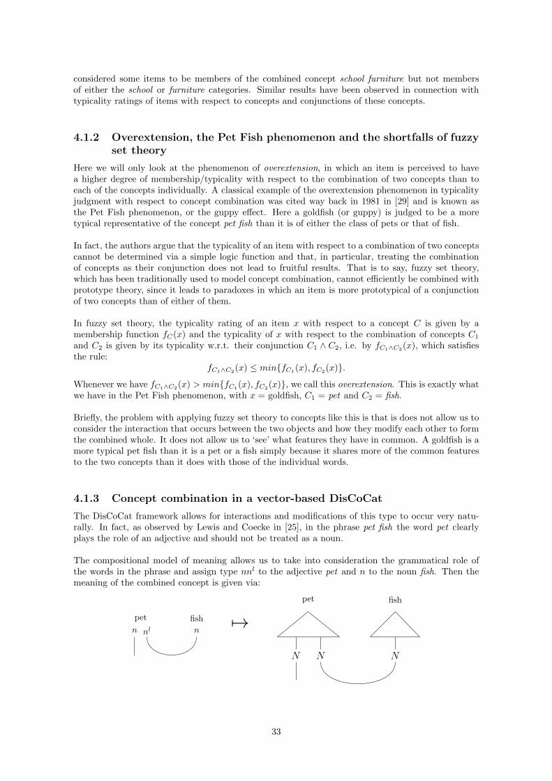
considered some items to be members of the combined concept school furniture but not membersof either the school or furniture categories. Similar results have been observed in connection withtypicality ratings of items with respect to concepts and conjunctions of these concepts.
4.1.2 Overextension, the Pet Fish phenomenon and the shortfalls of fuzzyset theory
Here we will only look at the phenomenon of overextension, in which an item is perceived to havea higher degree of membership/typicality with respect to the combination of two concepts than toeach of the concepts individually. A classical example of the overextension phenomenon in typicalityjudgment with respect to concept combination was cited way back in 1981 in [29] and is known asthe Pet Fish phenomenon, or the guppy e↵ect. Here a goldfish (or guppy) is judged to be a moretypical representative of the concept pet fish than it is of either the class of pets or that of fish.
In fact, the authors argue that the typicality of an item with respect to a combination of two conceptscannot be determined via a simple logic function and that, in particular, treating the combinationof concepts as their conjunction does not lead to fruitful results. That is to say, fuzzy set theory,which has been traditionally used to model concept combination, cannot e�ciently be combined withprototype theory, since it leads to paradoxes in which an item is more prototypical of a conjunctionof two concepts than of either of them.
In fuzzy set theory, the typicality rating of an item x with respect to a concept C is given by amembership function fC(x) and the typicality of x with respect to the combination of concepts C
1
and C2
is given by its typicality w.r.t. their conjunction C1
^ C2
, i.e. by fC1^C2(x), which satisfiesthe rule:
fC1^C2(x) min{fC1(x), fC2(x)}.
Whenever we have fC1^C2(x) > min{fC1(x), fC2(x)}, we call this overextension. This is exactly whatwe have in the Pet Fish phenomenon, with x = goldfish, C
1
= pet and C2
= fish.
Briefly, the problem with applying fuzzy set theory to concepts like this is that is does not allow us toconsider the interaction that occurs between the two objects and how they modify each other to formthe combined whole. It does not allow us to ‘see’ what features they have in common. A goldfish is amore typical pet fish than it is a pet or a fish simply because it shares more of the common featuresto the two concepts than it does with those of the individual words.
4.1.3 Concept combination in a vector-based DisCoCat
The DisCoCat framework allows for interactions and modifications of this type to occur very natu-rally. In fact, as observed by Lewis and Coecke in [25], in the phrase pet fish the word pet clearlyplays the role of an adjective and should not be treated as a noun.
The compositional model of meaning allows us to take into consideration the grammatical role ofthe words in the phrase and assign type nnl to the adjective pet and n to the noun fish. Then themeaning of the combined concept is given via:
n nl n
N N N
pet fish
pet fish 7!
33

(1N ⌦ "N )⇣����!pet-adj ⌦
��!fish
⌘
If we take the adjective to be given by����!pet-adj =
Pij ↵ij
�!ni ⌦ �!nj , with respect to the same basis
vectors {�!ni}i as for the noun��!fish =
Pk �k
�!nk, we obtain the meaning of the phrase to be:
(1N ⌦ "N )⇣����!pet-adj ⌦
��!fish
⌘= (1N ⌦ "N )
0
@X
ij
↵ij�!ni ⌦�!nj ⌦
X
k
�k�!nk
1
A
=X
ijk
↵ij�k�!nih�!nj |�!nki
=X
ij
↵ij�!nih�!nj |
��!fishi.
In fact, the approach taken in [25] is to simplify the model by taking the adjective to be a sum ofits attributes, in accordance with [19] and forcing it back into its assigned dimension by using the
Frobenius copy � operator. In other words, set����!pet-adj =
Pi�!ei =
Pi ↵
peti
�!ni where�!ei are the words
that co-occur with the adjective, i.e. in this case mostly nouns that are modified by it. Then toreturn the adjective back to the appropriate dimension, we take:
����!pet-adjcopy = �(
����!pet-adj) =
X
i
↵peti
�!ni ⌦�!ni .
Then the meaning of pet fish becomes:
(1N ⌦ "N )⇣����!pet-adjcopy ⌦
��!fish
⌘=X
i
↵peti
�!ni h�!ni |��!fishi =
����!pet-adj �
��!fish,
where � is the pointwise product. So we get that pet fish is simply a fish whose each feature is mod-ified by the corresponding feature of the adjective pet, where the adjective itself takes into accountthe arguments that go with it.
The idea then is the following. After computing the vector for the concept pet fish, the vector forgoldfish is compared to it, and also to the vectors for pet and fish individually. This is done via thesymmetric cosine similarity measure.
Definition 23. Let �!x = (x1
, . . . xn)T and �!y = (y
1
, . . . , yn)T be two vectors of the same dimension.
Then the cosine between them is given by:
cos (�!x ,�!y ) =�!x ·�!y
||�!x || · ||�!y || =P
i xi ⇥ yipPi x
2
i
pPi y
2
i
.
Below is a summary of the toy example performed in [25], exactly as it appears in the paper.
Suppose that the nouns pet, fish, goldfish, cat, dog, shark are modeled with respect to the hand-chosenset of salient features:
{������!cared-for,
����!vicious,
����!fluffy,
���!scaly,
��������!lives-in-sea,
����������!lives-in-house},
as shown in the table below:
pet fish goldfish cat dog shark
cared-for 1 0.2 0.7 0.9 0.9 0vicious 0.2 0.8 0 0.2 0.4 1flu↵y 0.7 0 0 0.9 0.7 0scaly 0. 2 1 1 0 0 1lives in sea 0 0.8 0 0 0 1lives in house 0.9 0.3 0.9 0.9 0.9 0
Take����!pet-adj =
�!dog +
�!cat +
�����!goldfish = (0.5, 0.6, 1, 1, 2.7)T . Then the cosine similarities between the
words are as follows:
34

goldfish cat dog shark
pet(noun) 0.7309 0.9816 0.9809 0.1497fish 0.5989 0.2500 0.3292 0.9670pet(adj) fish 0.9379 0.5550 0.6225 0.5846
Thus, as we can see from the table, the similarity between goldfish and pet fish is indeed higher thanthat between goldfish and pet or fish individually.
4.1.4 Transition to a density-matrix based environment in CPM(FHilb)
Following the same train of thought, we introduce the density matrix for the adjective pet to bethe sum of the density matrices corresponding to the pet nouns that the adjective modifies, i.e. wethink of the adjective pet as being a mixture of its arguments. The main motivation behind makingthe switch to a density-matrix based representation is that it allows us to think of the adjective petas a mixture of its constituents, thus making the interactions between their salient features moreprominent. It also allows for asymmetric measures of similarity to be applied to the matrices.
Suppose that the density matrices which correspond to pure states for the nouns cat, dog, fish andgoldfish are given by:
pdogq = |dogihdog| = X
i
↵i |nii!0
@X
j
↵jhnj |
1
A =X
ij
↵i↵j |niihnj |
pcatq = |catihcat| = X
k
�k |nki!
X
l
�lhnl|!
=X
kl
�k�l |nkihnl|
pgoldfishq = |goldfishihgoldfish| = X
p
�p |npi!
X
q
�qhnq|!
=X
pq
�p�q |npihnq|
pfishq = |fishihfish| = X
t
�t |nti!
X
u
�u |nui!
=X
tu
�t�u |ntihnu|
And the mixed state for the adjective pet is given by the density matrix:
ppet-adjq = pdogq+ pcatq+ pgoldfishq
=X
ij
↵i↵j |niihnj |+X
kl
�k�l |nkihnl|+X
pq
�p�q |npihnq|
=X
rs
Cpetrs |nrihns|.
As before, in order to compute the meaning of pet fish, we will first copy the adjective and thencombine it with the noun with the "-map. Diagrammatically, we get:
N
N N
N
N
N N
N N N N
N
N
N
N
pet fishpet fish
CPM(FHilb) FHilb
35
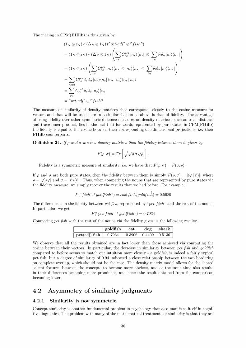
The meaing in CPM(FHilb) is thus given by:
(1N ⌦ "N ) � (�N ⌦ 1N ) (ppet-adjq⌦ pfishq)
= (1N ⌦ "N ) � (�N ⌦ 1N )
X
rs
Cpetrs |nrihns| ⌦
X
tu
�t�u |ntihnu|!
= (1N ⌦ "N )
X
rs
Cpetrs |nrihns|⌦ |nrihns| ⌦
X
tu
�t�u |ntihnu|!
=X
rstu
Cpetrs �t �u |nrihns| hnr |ntihns |nui
=X
rs
Cpetrs �r �s |nrihns|
= ppet-adjq� pfishq
The measure of similarity of density matrices that corresponds closely to the cosine measure forvectors and that will be used here in a similar fashion as above is that of fidelity. The advantageof using fidelity over other symmetric distance measures on density matrices, such as trace distanceand trace inner product, lies in the fact that for words represented by pure states in CPM(FHilb)the fidelity is equal to the cosine between their corresponding one-dimensional projections, i.e. theirFHilb counterparts.
Definition 24. If ⇢ and � are two density matrices then the fidelity between them is given by:
F (⇢,�) = Tr
qp⇢ �
p⇢
�.
Fidelity is a symmetric measure of similarity, i.e. we have that F (⇢,�) = F (�, ⇢).
If ⇢ and � are both pure states, then the fidelity between them is simply F (⇢,�) = |h' | i|, where⇢ = |'ih'| and � = | ih |. Thus, when comparing the nouns that are represented by pure states viathe fidelity measure, we simply recover the results that we had before. For example,
F (pfishq, pgoldfishq) = cos(��!fish,
�����!goldfish) = 0.5989
The di↵erence is in the fidelity between pet fish, represented by ppet-fishq and the rest of the nouns.In particular, we get
F (ppet-fishq, pgoldfishq) = 0.7934
Comparing pet fish with the rest of the nouns via the fidelity gives us the following results:
goldfish cat dog shark
pet(adj) fish 0.7934 0.3906 0.4409 0.5136
We observe that all the results obtained are in fact lower than those achieved via computing thecosine between their vectors. In particular, the decrease in similarity between pet fish and goldfishcompared to before seems to match our intuition more closely - a goldfish is indeed a fairly typicalpet fish, but a degree of similarity of 0.94 indicated a close relationship between the two borderingon complete overlap, which should not be the case. The density matrix model allows for the sharedsalient features between the concepts to become more obvious, and at the same time also resultsin their di↵erences becoming more prominent, and hence the result obtained from the comparisonbecoming lower.
4.2 Asymmetry of similarity judgments
4.2.1 Similarity is not symmetric
Concept similarity is another fundamental problem in psychology that also manifests itself in cogni-tive linguistics. The problem with many of the mathematical treatments of similarity is that they are
36

inherently symmetric, especially when based on geometric reasoning. As exhibited in [40] experimen-tally, concept similarity is intrinsically asymmetric. In the same paper, Tversky argues that similarityjudgments should be treated as statements of the form ‘a is like b’ (which is usually di↵erent from ‘bis like a’ ), rather than ‘a and b are similar’. He further claims that “the direction of the asymmetryis determined by the relative salience of the stimuli; the variant is more similar to the prototype thanvice versa”.
In one of the experiments conducted in support of this claim, a group of test subjects is asked todecide which of a given pair of countries is more similar to the other one. The subjects had tochose between ‘Country A is similar to country B’ and ‘Country B is similar to country A’. In thisexperiment almost all of the subjects picked the phrase ‘North Korea is similar to China’ and not‘China is similar to North Korea’. The general observation was that given two countries which sharesome common features, the more prominent country (‘the prototype’) determined the direction of theasymmetry.
4.2.2 DisCoCat model to capture asymmetry
The distributional model of meaning framework provides us with a very natural environment formodeling this kind of asymmetry. We propose one way of doing this in FHilb. We choose thesentence space S to be one-dimensional truth theoretic and constant, i.e.,
�!1 everywhere, and model
the verb: is similar to with respect to the same basis vectors {�!ni}i as those used as context wordsfor the noun space N . Thus, the weights Cij for the verb
���������!is-similar-to =
X
ij
Cij�!ni ⌦
�!1 ⌦�!nj
⇠=X
ij
Cij�!ni ⌦�!nj
correspond to the number of times that a noun with salient feature ni occurs as the subject of theverb, while at the same time a noun with feature nj appears as its object. In reality, there is no reasonwhy in general we should have Cij = Cji, i.e. there is no reason why the verb is similar to should besymmetric. This asymmetry of the verb propagates through the sentence via the meaning map andresults in an output that di↵erentiates between the two sentences ‘China is similar to North Korea’and ‘North Korea is similar to China’. Note that by essentially eliminating the sentence space, weforce the output of the meaning map applied to these sentences to be a real number. Then the ideais that the greater number of the two corresponds to the more ‘likely’ sentence.
To make this idea concrete, we will consider a toy example. Note that all the weights in this examplewere created by hand and by intuition and are vaguely based on widely available facts but not ex-tracted from a corpus or supported by any kind of experimental evidence. Empirical evidence wouldbe required to verify the results.
The assumption here is that the countries China and North Korea are judged against a set of contextwords which correspond to salient features that could in practice be extracted from a corpus or elicitedfrom human trials. We will take the context words to be the following set:
{�!big,
������!populous,
�������!prominent,
������!affluent,
��������!East Asian,
��������!communist,
��������!militarised}.
The vectors for����!China =
Pi ↵
Chi
�!ni and���������!NorthKorea =
Pl ↵
NKl
�!nl are summarised in the followingtable:
China North Korea
big 0.9 0.3populous 1 0.4prominent 0.8 0.4a✏uent 0.5 0.2East Asian 1 1communist 0.6 0.8militarised 0.6 0.9
37

and the weights Cij for the verb���������!is-similar-to are given by:
big populous prominent a✏uent East Asian communist militarised
big 0.7 0.5 0.6 0.5 0.1 0.2 0.3populous 0.2 0.7 0.8 0.5 0.6 0.1 0.2prominent 0.4 0.5 0.7 0.8 0.4 0.1 0.3a✏uent 0.6 0.6 0.8 0.6 0.3 0.2 0.2East Asian 0.3 0.7 0.6 0.3 0.7 0.1 0.4communist 0.1 0.1 0.2 0.1 0.3 0.8 0.5militarised 0.2 0.1 0.4 0.2 0.2 0.1 0.5
Next we compute the meanings of the two sentences:
� = China is similar to North Korea. = North Korea is similar to China.
in FHilb according to the diagram:
N N S N N
country A is similar to country B
with meaning map "N ⌦ 1S ⌦ "N , which we can simply treat as f = "N ⌦ "N and forget about thesentence space. The meanings are then:
f(�) = ("N ⌦ "N )
0
@X
i
↵Chi
�!ni ⌦X
jk
Cjk�!nj ⌦�!nk ⌦
X
l
↵NKl
�!nl
1
A
=X
ik
↵Chi Cik ↵
NKk ⇡ 8.1
f( ) = ("N ⌦ "N )
0
@X
l
↵Nkl
�!nl ⌦X
jk
Cjk�!nj ⌦�!nk ⌦
X
i
↵Chi
�!ni
1
A
=X
ij
↵NKj Cji ↵
Chi ⇡ 9.1
Thus, as expected, f( ) > f(�).
Discussion
As observed in the above example, this very simple model seems to be applicable to the task ofmodeling asymmetry and there is no reason not to be believe that it can be extended to all sortsof examples and possible scenarios. What enables us to do this is the intrinsic asymmetry of verbs,even the auxiliary verb to be, and the fact that the compositionality of the systems allows for thisasymmetry to propagate through the sentence and result in a di↵erent meaning outputs to ‘Noun1verb Noun2’ and ‘Noun2 verb Noun1’.
The same idea can easily be extended to the category CPM(FHilb) by making the transition fromnoun vectors to matrices. However, the results obtained would provide only a marginal improvementat the expense of increased complexity.
An alternative solution that eliminates the need to use the verb is similar to or any of its synonymswould be to model the two concepts (countries) as mixed states in CPM(FHilb) and compare them via
38

an asymmetric measure of similarity on density matrices that produces quantitative results. We willintroduce one such measure in the next chapter and discuss towards the end how it could potentiallybe implemented on the task in future work.
39

Chapter 5
P-Hyponymy
5.1 Introduction
As we already mentioned, one of the greatest advantages of transitioning to the CPM(FHilb) categoryand using density matrices instead of vectors lies in the possibilities for applying asymmetric measuresand orders on the matrices. One such measure was developed in [2] and was utilised for the taskof determining word hyponymy. Here we will introduce a new and simpler measure, which not onlyallows for exhibiting hyponymy relations between concepts, but also enables us to quantify them.We will see how this works on the level of sentences and how it can be generalised to apply to allfamiliar grammatical structures within the DisCoCat framework. Finally, we will briefly considerwhat happens when we try to implement variations of this measure to model other phenomena, suchas those mentioned in Chapter 4.
5.1.1 What is hyponymy?
In simplest terms possible, hyponymy is a ‘is-a-type-of ’ relation between two concepts X (the hy-ponym) and Y (the hypernym), i.e. X and Y are in a hyponym-hypernym relation if X is a type of Y.For example, a Siamese cat is a type of cat. However, in reality, hyponymy is an incredibly complexlinguistic phenomenon and has no universally agreed upon rigorous mathematical definition.
Examining the various possible characterisations of hyponymy even on a superficial level is well be-yond the scope and intention of this work. The interested reader is referred to [10]. Broadly speaking,there are several di↵erent ways of defining this linguistic concept, including various extensional andintentional logic, collocational, componential, and prototype-theoretic approaches. Each of these hascertain advantages and disadvantages over the others, and there are inevitably always cases of real-lifeuses of hyponymy that each of them fails to capture properly, or at all.
The definition that will be assumed here will be more or less a simplified version of the prototype-theoretic one. As we said at the beginning, the hyponym-hypernym relation X-Y is one of the formX is a type/kind/sort of Y. To make this a bit more precise, we first need to specify that X and Ycan be any pair of concepts expressible via words or phrases of the same grammatical type, and interms of a pre-defined set of salient features. Then we will say that X is a hyponym of Y and thatY is a hypernym of X if the features of X are contained in those of Y.
It will be assumed below that whenever we write ‘X-Y pair’, we mean a pair of concepts where Xis a hyponym of Y. Similarly, when we say that ‘we have hyponymy’ between X and Y, this will beunderstood to mean that X is a hyponym of Y.
5.1.2 Graded hyponymy
Note that, clearly, some X-Y pairs better exemplify hyponymy than others. For example, the pairapple - fruit as opposed to tomato - fruit. This leads to another concept, that of typicality, orprototypicality. Loosely speaking, if the hyponymy bond between X and Y is su�ciently strong,
40
then we can think of them as being in a ‘is-a-typical ’ kind of relationship, rather than a ‘is-a-type-of ’one. On the other hand, if we have very ‘weak’ hyponymy, then we can think of X as being just amember of the class Y. Thus, while this is not at all rigorous from a linguistic point of view, it willbe useful for us to consider membership, hyponymy and typicality as increasingly stronger versionsof the same concept, i.e. we will assume that membership hyponymy typicality. In fact, wewill unite these into the single new concept that we will call p-hyponymy, which will be a gradedversion of hyponymy that does not necessarily coincide entirely with the linguistic definition of theconcept.
We will not only be interested in whether or not X-Y is a hyponym-hypernym pair, but also in howstrong the hyponymy between these concepts is. The idea is that the stronger this hyponymy is, thecloser we get to having prototypicality. For example, a shinai is a hyponym to kendo weapon; in fact,a shinai is the prototypical kendo weapon. Hence, we expect to have very high hyponymy betweenthe two, as captured by the value of p. What we mean by that will be made precise below.
5.1.3 Using measures on density matrices for hyponymy
Modeling hyponymy in the DisCoCat framework was first considered by Balkir in [2] where she in-troduced an asymmetric similarity measure on density matrices based on quantum relative entropy,which can be used to translate hyponym-hypernym relations to the level of positive transitive sen-tences. This measure relies on a version of the Distributional Inclusion Hypothesis and, while it ispossible to make it quantitative, it is only considered in its qualitative version which induces a partialorder on density matrices. Our aim here will be to provide an alternative and simpler measure, rely-ing only on the properties of density matrices and the fact that they are the states in CPM(FHilb).This will enable us to order the words captured via the density matrices based on the strength oftheir relative hyponymy, i.e. in a quantitative fashion, as described by the idea of p-hyponymy. Wewill show how the order induced by the p-hyponymy can be lifted to the sentence level, not only forpositive transitive sentences, but for a much wider range of structures. In a sense, this measure willalso be more general than that in [2] as our definition of hyponymy is much more general.
5.1.4 Properties of hyponymy
Before proceeding with defining the concept of p-hyponymy, we will list a couple of properties ofhyponymy. We will show later that these can be captured by our new measure.
• Asymmetry. If X is a hyponym of Y, then this does not imply that Y is a hyponym of X.In fact, we may even assume that only one of these relationships is possible, and that they aremutually exclusive. For example, tchoukball is a type of sport and hence tchoukball-sport is ahyponym-hypernym pair. However, sport is definitely not a type of tchoukball.
• Pseudo-transitivity. If X is a hyponym of Y and Y is a hyponym of Z, then X is a hyponymof Z. For example, a Volkswagen is a type of car, and a car is a type of vehicle, so we havethe hyponym-hypernym pairs Volkswagen-car and car-vehicle. Then it is certainly true that aVolkswagen is a type of vehicle. However, the relationship between hyponyms becomes weakerwith the distance between them. A Volkswagen might sill be a vehicle, but is it definitely moreof a car, and similarly, the more general concept of a car is closer in meaning to the conceptof a vehicle than a Volkswagen is. This is why we call this pseudo transitivity. In a sense, thisimplies a hierarchical structure of hyponyms, where the further away we go from the lowesthyponym, the weaker the hyponymy. This is a natural consequence of the fact that in generala hypernym defines a broader category than its hyponyms.
5.2 Background definitions and results
Here we present some definitions and results that will be used later on.
Definition 25 (Positive semi-definite matrix). Let M 2 Mn(R) be a real symmetric n ⇥ n matrix.We say that M is positive semi-definite, and write M ⌫ 0, if for any column vector �!x 2 Rn it holds
41

that:�!x TM�!x � 0.
Note that �!x TM�!x = h�!x ,M�!x i, where h·, ·i : Rn⇥Rn ! R is the usual vector inner product on Rn.
• An alternative characterisation of positive semi-definiteness in terms of eigenvalues tells us thata square Hermitian matrix M is positive semi-definite i↵ all of its eigenvalues are non-negative.
• Note that density matrices can be characterised in terms of positive semi-definite matrices asdensity matrices are self-adjoint, positive semi-definite matrices with trace 1.
Proposition 1. The sum of an arbitrary number of positive scalar multiples of positive semi-definitematrices is positive semi-definite.
Proof. Fix n 2 N and let X1, . . . ,Xn be positive semi-definite matrices and ↵1
, . . .↵n be non-negative real numbers. Let �!x 2 Rn be an arbitrary non-zero vector and consider the inner producth�!x ,
Pi ↵iXi ·�!x i. By the linearity of the inner product, we have that:
*�!x ,
X
i
↵iXi ·�!x+
=X
i
↵i h�!x ,Xi ·�!x i .
Since for each j 2 [1, n], Xj is a positive semi-definite matrix, we have that each h�!x , Xj ·�!x i � 0and hence
Pi ↵i h�!x , Xi ·�!x i � 0.
Proposition 2. The following is a necessary condition for a Hermitian matrix A = (aij) to bepositive semi-definite: aii � 0, 8i, i.e. all the diagonal entries are non-negative.
5.3 P-Hyponyms
5.3.1 A new measure on density matrices
The measure of hyponymy that we described above and named p-hyponymy will be defined in termsof density matrices - the containers for word meanings. The idea is then to define a quantitative orderon the density matrices, which is not a partial order, but does give us an indication of the asymmetricrelationship between words. This is based on the partial order on the set of all square matrices givenby A B i↵ B �A ⌫ 0.
Definition 26 (P-hyponym). Let pAq and pBq be density matrix representations of the concepts Aand B respectively. We say that A is a p-hyponym of B for a given value of p in the range (0, 1] andwrite pAq 2p pBq if
pBq� p pAq ⌫ 0.
Remark. Note that such a p need not be unique or even exist at all. We will consider the interpre-tation and implications of this later on. Moreover, whenever we do have p-hyponymy between A andB, there is necessarily a largest such p.
Definition 27 (P-max hyponym). If A is a p-hyponym of B for any p 2 (0, 1], then there is necessarilya maximal possible such p. We denote it by pmax and define it to be the max value of p in the range(0, 1] for which we have pAq 2p pBq, in the sense that there does not exist q 2 (0, 1] s.t. q > p andpAq 2q pBq.
5.3.2 Interpretation of the values of p
The values of p in the p-hyponymy measure are meant to denote probabilities. The idea is that thecloser p is to 1, the stronger the hyponymy between A and B. That is to say, the closer A is to beingin a ‘is-a-typical ’ relationship with B. Clearly, the value of p is not unique for an A-B pair; however,p-max is always unique. This can be interpreted as giving us an upper bound of how close A canget to B, while at the same time indicating that it might not always be the case that A does getthat close to B. This might, for example, depend on the context in which the two concepts are used.A shinai may be a very strong p-max hyponym of kendo weapons in general, but exhibit a weaker
42

connection to the martial art in some context.
Below we give a brief justification of why the range of possible values of p makes sense.
Proposition 3 (P-hyponymy for p 0 is useless). It always holds that pAq 2p pBq if p 0.Therefore, the notion of p-hyponymy is useless for non-positive values of p.
Proof. Let p 0. Then
pAq 2p pBq () pBq� p pAq ⌫ 0 () pBq+ q pAq ⌫ 0 ,
where q = �p � 0. Since pAq and pBq are density matrices and hence positive semi-definite, and qis non-negative, we get by Proposition 1 that pBq+ q pAq ⌫ 0.
The next proposition justifies why we do not consider values of p exceeding 1. It turns out that wenever actually find ourselves in this situation. This makes sense intuitively, given our interpretationof the value of p as being a measure of proximity or a probability. If p = 1 is interpreted as beingabsolute hyponymy, or prototypicality, then we should expect to not be able to exceed this value.
Proposition 4. The value of p cannot exceed 1.
Note that we assume that the matrices we are comparing are always of the same dimension. Also,since the density matrices correspond to words or phrases in our model, we know that all of theirentries are non-negative, given the methods by which word meaning vectors are normally constructed.
Proof. Suppose that p-hyponymy were possible for values of p exceeding 1. Let p be such a valuefor which we have pAq 2p pBq, for some density matrices pAq and pBq. Then pBq � p pAq ⌫ 0.Define the matrix C = pBq � p pAq. By assumption, this matrix is positive semi-definite and hasdiagonal entries cii = bii�paii. Since a positive semi-definite matrix has only non-negative entries onits diagonal, by Proposition 2, we have that cii � 0 , 8i. Also, the matrices pAq and pBq have onlynon-negative entries, and in particular aii � 0 , 8i and bii � 0 , 8i. Moreover, since they are densitymatrices, we have
Pi bii =
Pj ajj = 1. Thus,
(cii � 0 8i) =) (bii � paii 8i) =)X
i
bii � pX
j
ajj >X
j
ajj =) 1 > 1 ,
which is a contradiction.
The following observation relates to the property of words to be hyponyms of themselves in a trivialway. In other words, we expect that any word or concept should be an absolute hyponym of itself, inthe sense of being a 1-max hyponym of itself.
Proposition 5. Any word A is a 1-max hyponym of itself.
Proof. Let A be an arbitrary word with density matrix representation pAq . Then as pAq�pAq = p0qand p0q is by definition a positive semi-definite matrix, we conclude that pAq 2
1
pAq, i.e. A is a1-hyponym of itself, and hence a 1-max hyponym of itself.
5.3.3 Extracting p-hyponymy values out of hyponym-hypernym pairs
We will make the assumption that hypernyms can be expressed in terms of their hyponyms, whichis, again, not completely rigorous from a linguistic point of view, but is a valid assumption for ourpurposes nonetheless. For example, if all the hyponyms of the hypernym sport are tchoukball, volley-ball and pickleball, then we can think of the concept sport as being tchoukball+volleyball+pickleball.
In practice, one way of making use of this assumption is by representing the density matrix corre-sponding to sport as a mixture of the density matrices for the individual sports, weighted by thenumber of times that the given sport has co-occurred with the word sport in a large body of text orcorpus. This idea is somewhat similar to the way in which we sometimes represent collective nounsas a sum of their constituents in the vector-based model. The weights are generally normalised tobe between 0 and 1 and are not assumed to sum to 1. However, it will be more convenient for us to
43

assume that they do, i.e. to treat them as probabilities. We can always get rid of this assumptionby normalising the resulting matrix for sport so that it has trace 1 after we have already included allthe sports in it.
More generally, this works as follows. Suppose that pXiq are the density matrix representations forthe hyponyms of the word B. Then the density matrix for B is given by:
pBq =X
i
pi pXiq.
HereP
i pi = 1. To drop this assumption, we can define pB0q =
Pi qi pXiq to be the normalised
version of pBq with trace 1. We will always assume any density matrix we have is already normalised.
Proposition 6. Suppose that pAq 2 {pXiq}i, i.e that we have:
pBq = pjpAq+X
i 6=j
pi pXiq
ThenpAq 2p pBq ,
for any p pj.
Proof. Without loss of generality suppose that pBq = p1
pAq+P
i 6=1
pi pXiq and consider
⇠ = h�!x , (pBq� p pAq)�!x i for any p p1
.
We want to show that pAq 2p pBq, i.e. ⇠ � 0, 8�!x 6= 0. We have:
⇠ = h�!x , (pBq� p pAq)�!x i =*�!x ,
0
@(p1
pAq+X
i 6=1
pi pXiq)� p pAq
1
A�!x+
=
*�!x ,
0
@(p1
� p) pAq+X
i 6=1
pi pXiq
1
A�!x+
=
*�!x , (p
1
� p) pAq
�!x +X
i 6=1
pi pXiq�!x+
= h�!x , (p1
� p)pAq
�!x i+*�!x ,X
i 6=1
pi pXiq�!x+
= (p1
� p) h�!x , pAq
�!x i+X
i 6=1
pi h�!x , pXiq�!x i
By assumption, all of the pXiq and pAq are positive semi-definite matrices and all the pi are non-negative. For any choice of p s.t. p p
1
we have p1
� p � 0. Thus, for any such p we end up witha non-negative linear combination of non-negative quantities, i.e. a non-negative quantity. In otherwords, we have p-hyponymy.
The p-max value: Discussion and assumptions
From the above proof we notice that the value p1
definitely gives us p1
-hyponymy between A andB, but it is actually possible that there exists a value, say q, such that q > p
1
and for whichwe have q-hyponymy between A and B. Indeed, this happens whenever we have a q for which(p
1
� q) h�!x , pAq
�!x i � �P
i 6=1
pi h�!x , pXiq�!x i. Thus, p
1
may not be the maximum value for hy-ponymy between A to B. In practice, such a value can be determined by testing for numbers q 2 (0, 1],s.t. q > p
1
and for which the eigenvalues of the matrix pBq� q pAq are all non-negative. This followsfrom the equivalent characterisation of positive semi-definiteness in terms of eigenvalues. If pAq isnot in the span of the rest of the pXiq then we do get that the maximum value of the hyponymy isp = p
1
. We will work under the assumption that this is always the case, i.e. that the co-hyponymsof a hypernym are independent of each other.
44

Now suppose that we drop the assumption that we have previous knowledge about all the hyponymsof B that are meant to go into the mixture that we use to define B, i.e. suppose that we do not knowthat pBq =
Pi pi pXiq, where pXiq are all the relevant hyponyms of B. Suppose that all we know
is that A is a hyponym of B. Can we still say anything about the actual strength of the hyponymybetween A and B?
According to our definition, starting only from the knowledge that A is a hyponym of B, we get thatpAq 2p pBq, for some p, and hence that pBq� p pAq ⌫ 0. So there exists some PSD matrix, say ⇢,such that pBq = p pAq+ ⇢. Then, similar to above, to determine the maximum possible value of p,we will need to test for values in the range (0, 1] for which the eigenvalues of the matrix pBq� p pAq
are all non-negative. So, in theory, we could find a maximal p which satisfies the definition of p-hyponymy between A and B. However, at present we have no way of knowing straight away whetherthis value is at all useful to us. In order to find out, a large-scale practical experiment would need tobe carried out to obtain empirical data that can give us an indication of the validity of this model.
Thus, in our applications and examples below, we will always work under the assumption that hy-pernyms are expressed in terms of a relevant set of independent hyponyms, in which case we have:
pAq 2pmax
pBq () pBq = pmax pAq+X
i
pi pXiq,
as in the previous proposition. Of course, all the results will also work for values of hyponymy belowthe maximal, but since the p-max hyponymy is what we are primarily interested in, we will assumethat we mean p-max hyponymy whenever we say p-hyponymy.
Note that all of the proofs below will also work even if we do not make the above assumption, butrather only work with the original definition that pAq 2p pBq () pBq � p pAq ⌫ 0 () pBq =p pAq + ⇢ for an unknown positive operator ⇢. This is because the idea behind all of the proofs isthat the morphisms of the category CPM(FHilb) are positive operators and hence preserve densitymatrices.
5.3.4 Properties of P-Hyponymy
The p-hyponymy measure satisfies some of the key properties of hyponymy, as described in the firstsection.
Property 1 (P-hyponymy is not symmetric). Given our assumption that hypernyms are expressedin terms of their hyponyms, the asymmetry of the hyponymy relation is satisfied by default.
Note, however, that we are also quantifying the hyponymy between the words and so it is possible tohave both A 2p B and B 2q A. In this case, if, say, p has a high value then q is bound to be veryclose to 0, and hence indicative of basically non-existent hyponymy. It is also generally not true that
(pAq 2p pBq and pBq 2p pAq) =) pAq = pBq
unless p = q = 1, i.e. A 2
1
B and B 2
1
A. Then we just have the standard partial order on squarematrices induced by the positive semi-definiteness and this implies that in this case we must haveA = B. In practice, this means that either A and B are the same word or completely overlappingsynonyms, assuming that such a thing is even possible.
This is exactly how we expect hyponyms to behave in real life. As an example, we expect pork tobe a p-hyponym of meat for a relatively high value of p, and meat to be a q-hyponym of pork for avery small value of q. We certainly do not expect this to imply an equivalence between pork and meat.
A key property of hyponymy in the linguistic sense is that its strength decreases with distance. Whatwe mean by that is that if concept A is a hyponym of concept B and B is a hyponym of C, then A isstill a hyponym of C, but weaker than the previous two, like in our vehicle-car-Volkswagen example.
Property 2. (P-hyponymy decreases with distance) Suppose that A is a p-hyponym of B and B is ap0-hyponym of C, i.e. pAq 2p pBq 2p0
pCq. Then A is a p00 � hyponym of C for p00 = p · p0, i.e.pAq 2p00
pCq.
45

Proof. From pAq 2p pBq 2p0pCq we get:
pAq 2p pBq () h�!x , (pBq� p pAq)�!x i � 0 () h�!x , pBq
�!x i � ph�!x , pAq
�!x i,
pBq 2p0pCq () h�!x , (pCq� p0 pBq)�!x i � 0 () h�!x , pCq
�!x i � p0h�!x , pBq
�!x i.Combining these, we get:
h�!x , pCq
�!x i � p0h�!x , pBq
�!x i � p0ph�!x , pAq
�!x i = p00h�!x , pAq
�!x i () pAq 2p00pCq.
To illustrate this property, consider the following example.
Example
Let {|e1
i, |e2
i, |e3
i, |e4
i} be the standard orthonormal basis for R4 and consider the words:
�����������!white chocolate =
X
i
↵i |nii,����������!milk chocolate =
X
j
�j |nji
����������!dark chocolate =
X
k
�k |nki,��!cake =
X
l
�l |nli
We take the basis vectors to correspond to the context words sweet, milky, spongy and high-calorieand intuitively give the following vector representations to our words, where each word is evaluatedagainst each property on a scale of 0 to 1.
white chocolate milk chocolate dark chocolate cake
sweet 0.8 0.8 0.5 0.6milky 0.7 0.5 0.3 0.1spongy 0 0 0 0.8high-calorie 0.7 0.6 0.8 0.5
We take the hypernyms chocolate and sweets to be given by:
pchocolateq =1
4pwhite chocolateq+
1
2pmilk chocolateq+
1
4pdark chocolateq
psweetsq =1
5pchocolateq+
4
5pcakeq
The first hyponymy that we are interested in is that of white chocolate to chocolate and the secondone is that of chocolate to sweets. An explicit calculation shows us that the maximum p for whichwe have:
pwhite chocolateq 2p pchocolateq0
BB@
0.6400 0.5600 0 0.56000.5600 0.4900 0 0.4900
0 0 0 00.5600 0.4900 0 0.4900
1
CCA 2p
0
BB@
0.5425 0.3775 0 0.48000.3775 0.2700 0 0.3325
0 0 0 00.4800 0.3325 0 0.4625
1
CCA
is exactly p = 0.25.Similarly, the largest p0 for which we get:
pchocolateq 2p0psweetsq
0
BB@
0.5425 0.3775 0 0.48000.3775 0.2700 0 0.3325
0 0 0 00.4800 0.3325 0 0.4625
1
CCA 2p0
0
BB@
0.3965 0.1235 0.3840 0.33600.1235 0.0620 0.0640 0.10650.3840 0.0640 0.5120 0.32000.3360 0.1065 0.3200 0.2925
1
CCA
is p0 = 0.2. Thus, we expect that the maximum value p00 for which we have:
pwhite chocolateq 2p00psweetsq
to be p00 = 0.25 ⇥ 0.2 = 0.05. Again, a straightforward direct calculation shows that this is indeedthe case.
46

5.4 P-Hyponymy lifted to the level of sentences
We will now consider what happens when we have two sentences such that one of them contains oneor more hyponyms of one or more words from the other. We will show that in this case the hyponymyis ‘lifted’ to the sentence level, and even the p-values are preserved in a very intuitive fashion. Afterconsidering a couple of specific sentence construction, we will generalise this result to account for abroad category of sentence patterns that work in the distributional compositional model.
5.4.1 P-Hyponymy in positive transitive sentences
Recall that a positive transitive sentence has the following diagrammatic representation in CPM(FHilb):
N N S
N
0N
0
subject verb object
Translated to FHilb:
N N
N
0S N N S
N
0N
0N
0
subject
verb
object
So the meaning of the sentence Subject verb object is given by:
("N ⌦ 1S ⌦ "N ) (psubjq⌦ pverbq⌦ pobjq) ,
where the epsilon and identity morphisms are those from CPM(FHilb). We will represent the subjectand object vectors in FHilb by:
��!subj =
X
i
↵subji
�!ni and�!obj =
X
j
�objj
�!nj .
Their corresponding density matrix representations are given by:
psubjq =X
ik
↵subji ↵subj
k |niihnk| and pobjq =X
jl
�objj �obj
l |njihnl|.
Finally, let the verb be given by:
verb =X
rs
Cverbrs |nri|si|nsi.
Its density matrix is:
pverbq =
X
rs
Cverbrs |nri|si|nsi
! X
pq
Cverbpq hnp|hs0|hnq|
!=X
rspq
Cverbrs Cverb
pq |nrihnp|⌦|sihs0|⌦|nsihnq|
47

Relationship between sentences of the type ‘A verb C ’ and ‘B verb D’,where pAq 2p pBq and pCq 2q pDq
We will assume that the sentence space, i.e. the vector space corresponding to S, is not truth-theoreticand that hypernyms are always represented in terms of their hyponyms, as before.
Theorem 1. Let A, B, C and D be nouns with corresponding density matrix representations pAq,pBq, pCq and pDq, such that A is p-hyponym of B and C is a q-hyponym of D, in the sense that:
pBq = p pAq+X
i
pi pXiq and pDq = q pCq+X
j
qj pYjq.
Then we have that:' (A verb C) 2pq ' (B verb D) ,
where ' = "N ⌦ 1S ⌦ "N is the sentence meaning map for positive transitive sentences.
Proof. Let the density matrix corresponding to the verb be given by pZq. Then we can write themeanings of the two sentences as:
' (A verb C ) = ' (pAq⌦ pZq⌦ pCq) = ("N ⌦ 1S ⌦ "N ) (pAq⌦ pZq⌦ pCq)
' (B verb D) = ' (pBq⌦ pZq⌦ pDq) = ("N ⌦ 1S ⌦ "N ) (pBq⌦ pZq⌦ pDq)
Substituting pBq = p pAq +P
i pi pXiq and pDq = q pCq +P
j qj pYjq in the expression for themeaning of B verb D, we get:
'(pBq⌦ pZq⌦ pDq) = ("N ⌦ 1S ⌦ "N ) (pBq⌦ pZq⌦ pDq)
= '
0
@ p pAq+
X
i
pi pXiq
!⌦ pZq⌦
0
@q pCq+X
j
qj pYjq
1
A
1
A
= '
0
@pq (pAq⌦ pZq⌦ pCq) + p
0
@pAq⌦ pZq⌦
X
j
qjpYjq
1
A
+X
i
pipXiq⌦ pZq⌦
0
@X
j
qjpYjq+ q pCq
1
A
1
A
= '
0
@p
0
@pAq⌦ pZq⌦
X
j
qjpYjq
1
A+X
i
pipXiq⌦ pZq⌦
0
@X
j
qjpYjq+ q pCq
1
A
1
A
+ pq ' (pAq⌦ pZq⌦ pCq)(5.1)
Consider '(pBq⌦ pZq⌦ pDq)� pq '(pAq⌦ pZq⌦ pCq). We get:
'
0
@p
0
@pAq⌦ pZq⌦
X
j
qjpYjq
1
A+X
i
pipXiq⌦ pZq⌦
0
@X
j
qjpYjq+ q pCq
1
A
1
A
= pX
j
qj '(pAq⌦ pZq⌦ pYjq) +X
i
X
j
piqj'(pXiq⌦ pZq⌦ pYjq) + qX
i
pi '(pXiq⌦ pZq⌦ pCq)
(5.2)
Since pXiq, pYjq, pZq, pAq and pCq are all density matrices, all of the following are also densitymatrices: '(pXiq⌦ pZq⌦ pYjq), '(pAq⌦ pZq⌦ pYjq), '(pXiq⌦ pZq⌦ pCq). This is because we areworking in the CPM(FHilb) category and the meaning map ' is a completely positive map, whichmeans that it sends density matrices to density matrices. Moreover, all of the scalars pi, qj , p, q arenon-negative. Thus, (5.2) is a sum of non-negative scalar multiples of positive semi-definite matrices,and as such is positive semi-definite itself, by Proposition 1. We conclude that:
'(pBq⌦ pZq⌦ pDq)� pq '(pAq⌦ pZq⌦ pCq) ⌫ 0,
48

and so'(pAq⌦ pZq⌦ pCq) 2pq '(pBq⌦ pZq⌦ pDq).
Now suppose that all we know is that pAq 2p pBq and pCq 2q pDq. Then we can write
pBq = p pAq+ � and pDq = q pCq+ µ,
for positive operators � and µ. Then the exact same proof with � in place ofP
i pi pXiq and µ inplace of
Pj qj pYjq tells us that ' (A verb C) 2pq ' (B verb D). In particular, this applies to the case
where p = pmax and q = qmax are the maximum hyponymy values for the two hyponym-hypernympairs.
Two special cases of the above result occur when we take either the subjects or the objects of thetwo sentences to be the same, i.e pAq = pBq or pCq = pDq.
Corollary 1. Let A, B, C be nouns with corresponding density matrix representations pAq, pBq,pCq and such that pBq = p pAq+
Pi pi pXiq. Then we have that:
' (A verb C) 2p ' (B verb C) ,
where ' = "N ⌦ 1S ⌦ "N is the sentence meaning map.
Proof. This is just a special case of our theorem with pCq = pDq and q = 1. Then (5.2) abovebecomes simply:
'(pBq⌦ pZq⌦ pCq)� p'(pAq⌦ pZq⌦ pCq) =X
i
pi '(pXiq⌦ pZq⌦ pCq) ,
which is a positive semi-definite matrix, and thus '(pAq⌦ pZq⌦ pCq) 2p '(pBq⌦ pZq⌦ pCq).
Corollary 2. Let A, C, D be nouns with corresponding density matrix representations pAq, pCq,pDq and such that pDq = p pCq+
Pj qj pYjq. Then we have that:
' (A verb C) 2p ' (A verb D) ,
where ' = "N ⌦ 1S ⌦ "N is the sentence meaning map.
Proof. Similar to above.
Again, these results also work if we just have that pAq 2p pBq or pCq 2p pDq without any furtherassumption of knowledge about the representation of the hypernyms.
Examples of p-hyponymy in positive transitive sentences
Example 1
We assumed that the sentence space S is not truth-theoretic. The following example illustrates whathappens to positive transitive sentence hyponymy if we take a truth-theoretic approach to sentencemeaning, i.e. if we take the sentence space to be one- or two-dimensional truth-theoretic.
Suppose that our sentence space S is 1-dimensional, with its single non-trivial vector being�!1 .
We will take�!1 to stand for True and
�!0 for False. The sentences we will consider are:
A := Annie likes holidays.B := Students like holidays.
Let the vector space for the subjects of the sentences be R3 = SpanR{⇣1
0
0
⌘,⇣0
1
0
⌘,⇣0
0
1
⌘}, where:
����!Annie = |e
1
i =
0
@100
1
A ,���!Betty = |e
2
i =
0
@010
1
A ,���!Chris = |e
3
i =
0
@001
1
A .
49

Let the object vector space be Rn for some arbitrary n 2 N, where we take |n1
i to be the standard
basis vector for Rn with 1 in the first position and 0 elsewhere. Let�����!holidays = |n
1
i. We will treatthe concept students as being a hypernym of the individual students in our universe. In other words,
pstudentsq =1
3pAnnieq+
1
3pBettyq+
1
3pChrisq =
1
3|e
1
ihe1
|+ 1
3|e
2
ihe2
|+ 1
3|e
3
ihe3
|.
Finally, let the verb enjoy 2 R3 ⌦ S ⌦ Rn be given by enjoy =P
(i,j)2R|eii|nji, where
R = Renjoy
= {(i, j)| |eii enjoys |nji},
in the style of [7]. The corresponding density matrix for the verb is then:
penjoyq =X
(i,j)2R(r,s)2R
|eiiher|⌦ |njihns|.
Suppose that Annie and Betty are known to enjoy holidays, while Chris does not. Then the aboveset becomes simply R = {(1, 1), (2, 1)}.
Clearly, we have that pAnnieq 2pmax
pstudentq for pmax = 1
3
, since this is the maximum value of pfor which we have pstudentq� p pAnnq ⌫ 0, where:
pstudentq� 1
3pAnnieq =
0
@1
3
0 00 1
3
00 0 1
3
1
A� 1
3
0
@1 0 00 0 00 0 0
1
A =
0
@0 0 00 1
3
00 0 1
3
1
A .
We will see that the p-hyponymy for p = 1
3
does translate into p-hyponymy of sentence pAq tosentence pBq. However, we will also observe that this will no longer be the maximum value of p forwhich we have sentence hyponymy. First of all, consider the meanings of the two sentences:
pAq = ("N ⌦ 1S ⌦ "N )(pAnnieq⌦ penjoyq⌦ pholidaysq)
= ("N ⌦ 1S ⌦ "N )
0
BB@|e1
ihe1
|⌦X
(i,j)2R(r,s)2R
|eiiher|⌦ |njihns|⌦ |n1
ihn1
|
1
CCA
=X
(i,j)2R(r,s)2R
he1
|eiihe1|erihn1
|njihn1
|nsi =X
(i,j)2R(r,s)2R
�1i �1r �1j �1s =
X
(1,1)2R(1,1)2R
1 = 1
(5.3)
pBq = ("N ⌦ 1S ⌦ "N ) (pstudentq⌦ penjoyq⌦ pholidaysq)
= ("N ⌦ 1S ⌦ "N )
0
BB@1
3(|e
1
ihe1
|+ |e2
ihe2
|+ |e3
ihe3
|)⌦X
(i,j)2R(r,s)2R
|eiiher|⌦ |njihns|⌦ |n1
ihn1
|
1
CCA
=1
3
0
BB@X
(i,1)2R(r,1)2R
he1
|eiihe1|eri+X
(i,1)2R(r,1)2R
he2
|eiihe2|eri+X
(i,1)2R(r,1)2R
he3
|eiihe3|eri
1
CCA
=1
3
0
BB@X
(i,1)2R(r,1)2R
�1i�1r +
X
(i,1)2R(r,1)2R
�2i�2r +
X
(i,1)2R(r,1)2R
�3i�3r
1
CCA
=1
3
0
@X
(1,1)2R
1 +X
(2,1)2R
1 + 0
1
A =1
3⇥ 2 =
2
3
(5.4)
50
Clearly, we have that pAq 2p pBq for p = 1
3
, as 2
3
� 1
3
⇥ 1 � 0, but this is not the maximumvalue of p for which this p-hyponymy holds. The max value for which this works is p = 2
3
. Thereason why this happens is that when we work with a truth-theoretic sentence space, the meaningsof the sentences that we obtain in the end are trivial density matrices, i.e just one-dimensional,and hence they do not capture all the information that a non-trivial matrix can. In a sense, insteadof obtaining a real density matrix meaning of the sentences, we just get the traces of density matrices.
Example 2: Simple case of object hyponymy
We now give a simple case with a non-truth-theoretic sentence space, in which we show that thep-hyponymy of the objects of two sentences translates into p-hyponymy between the sentences, andthat the maximality of the value of p is also preserved.
Let m 2 N, m > 2 be such that {ni}mi=1
is a collection of standard basis vectors for Rm. We will usethe nouns:
����!Gretel = |n
1
i,��������!gingerbread = |n
2
i,��!cake = |n
3
i,������!pancakes = |n
4
i,
with corresponding pure density matrices:
pGretelq = |n1
ihn1
|, pgingerbreadq = |n2
ihn2
|, pcakeq = |n3
ihn3
|, ppancakesq = |n4
ihn4
|
Let the mixed density matrix corresponding to the hypernym sweets be given by:
psweetsq =1
10|n
2
ihn2
|+mX
i=3
pi |niihni|.
Our object and subject vector space will be Rm and for the sentence space we take S = Rm ⌦ Rm.We take the verb like to be given by like 2 Rm ⌦ S ⌦ Rm ,
like =X
jk
Clikejk |nji|nji|nki|nki,
where the coe�cients Cjk give us the weight with which |nji likes |nki.For the rest of this example, we will adopt the following abuse of notation for the purpose of brevity:
|sjki = |nji|nki, hsjk| = hnj |hnk|, |sijihskl| = |niihnk|⌦ |njihnl|.
Then the density matrix representation of our verb becomes:
plikeq =
0
@X
jk
Clikejk |nji|sjki|nki
1
A
0
@X
lp
Clikelp hnl|hslp|hnp|
1
A
=X
jklp
Clikejk Clike
lp |njihnl|⌦ |sjkihslp|⌦ |nkihnp|.(5.5)
We will consider the following two sentences:
A := Gretel likes sweets.B := Gretel likes gingerbread.
Let the corresponding (density matrix) sentence meanings be given by:
pAq = ("N ⌦ 1S ⌦ "N ) (pGretelq⌦ plikeq⌦ psweetsq)
pBq = ("N ⌦ 1S ⌦ "N ) (pGretelq⌦ likeq⌦ pgingerbreadq)(5.6)
Observe that
pgingerbreadq 2p psweetsq for p 1
10.
51

In particular, we have pmax-hyponymy between gingerbread and sweets for pmax = 1
10
. We will nowshow that this hyponymy translates to the sentence level, as by Corollary 2. With ' = "N⌦1S⌦"N ,we have,
pAq = '
0
@|n1
ihn1
| ⌦X
jklp
Clikejk Clike
lp |njihnl|⌦ |sjkihslp|⌦ |nkihnp| ⌦
1
10|n
2
ihn2
|+mX
i=3
pi|niihni|!1
A
=1
10'
0
@|n1
ihn1
| ⌦X
jklp
Clikejk Clike
lp |njihnl|⌦ |sjkihslp|⌦ |npihnp| ⌦ |n2
ihn2
|
1
A+
+ '
0
@|n1
ihn1
| ⌦X
jklp
Clikejk Clike
lp |njihnl|⌦ |sjkihslp|⌦ |nkihnp| ⌦mX
i=3
pi |niihni|
1
A
pBq = '
0
@|n1
ihn1
| ⌦X
jklp
Clikejk Clike
lp |njihnl|⌦ |sjkihslp|⌦ |nkihnp| ⌦ |n2
ihn2
|
1
A
(5.7)
We claim that the maximum p-hyponymy between pBq and pAq is achieved for p = 1
10
. In otherwords, this is the maximum value of p for which we have pBq 2p pAq, i.e. pAq� p pBq ⌫ 0.To see this, consider pAq� 1
10
pBq. We get:
("N ⌦ 1S ⌦ "N )
0
@|n1
ihn1
| ⌦X
jklp
Clikejk Clike
lp |njihnl|⌦ |sjkihslp|⌦ |nkihnp| ⌦mX
i=3
pi |niihni|
1
A
=X
ijklp
Clikejk Clike
lp pi hn1
|njihn1
|nlihnk|niihnp|nii |sjkihslp|
=X
ijklp
Clikejk Clike
lp pi �1j�1l�ik�ip |sjkihslp|
=mX
i=3
Clike1i Clike
1i pi |s1iihs1i|
=mX
i=3
�Clike
1i
�2
pi |n1
ihn1
|⌦ |niihni|
(5.8)
Now suppose that Gretel is the only object in our universe that likes sweets and that she onlylikes pancakes, cakes and gingerbread, all with equal weights, which we take to be 1
3
, i.e. we let:
Clikejk =
(1
3
if j = 1, k 2 {2, 3, 4}0 o.w.
Then (5.8) above becomes simply 1
9
(p3
|n1
ihn1
|⌦ |n3
ihn3
|+ p4
|n1
ihn1
|⌦ |n4
ihn4
|). Note that this isisomorphic to 1
9
(p3
|n3
ihn3
|+ p4
|n4
ihn4
|), and that the former is a positive semi-definite matrix ifand only if the latter is. Alternatively, to simplify this example we could have just taken the object
vector space to be one-dimensional and consisting only of Gretel, in which case����!Gretel =
�!1 and we
get the same outcome.
Since |n3
ihn3
| and |n4
ihn4
| are pure state and p3
and p4
are non-negative real numbers, we get thatthe matrix p
3
|n3
ihn3
|+ p4
|n4
ihn4
| is positive semi-definite, which is what we claimed.
It is easy to see that for any other value of p below 1
10
, we would have also obtained a positivesemi-definite matrix upon computing pAq� ppBq.
Example 4
Now suppose that the subject and object vector spaces are two-dimensional and spanned by⇣1
0
⌘and
⇣0
1
⌘. For convenience, we denote these vectors by |e
1
i and |e2
i respectively when dealing with the
52
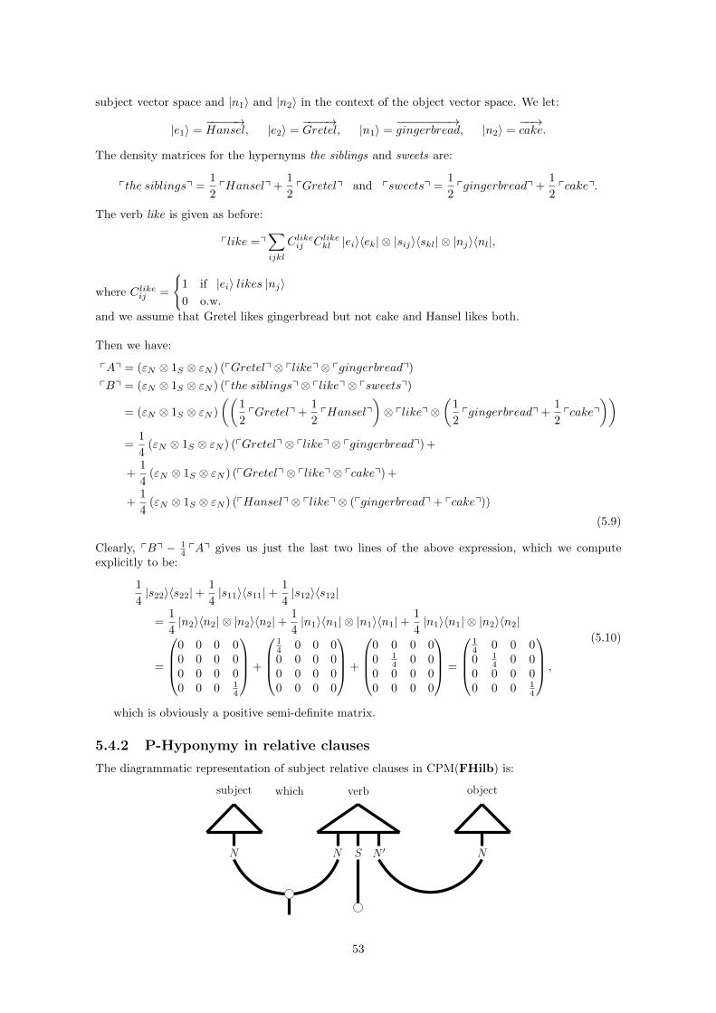
subject vector space and |n1
i and |n2
i in the context of the object vector space. We let:
|e1
i =�����!Hansel, |e
2
i =����!Gretel, |n
1
i =��������!gingerbread, |n
2
i =��!cake.
The density matrices for the hypernyms the siblings and sweets are:
pthe siblingsq =1
2pHanselq+
1
2pGretelq and psweetsq =
1
2pgingerbreadq+
1
2pcakeq.
The verb like is given as before:
plike =q
X
ijkl
Clikeij Clike
kl |eiihek|⌦ |sijihskl|⌦ |njihnl|,
where Clikeij =
(1 if |eii likes |nji0 o.w.
and we assume that Gretel likes gingerbread but not cake and Hansel likes both.
Then we have:
pAq = ("N ⌦ 1S ⌦ "N ) (pGretelq⌦ plikeq⌦ pgingerbreadq)
pBq = ("N ⌦ 1S ⌦ "N ) (pthe siblingsq⌦ plikeq⌦ psweetsq)
= ("N ⌦ 1S ⌦ "N )
✓✓1
2pGretelq+
1
2pHanselq
◆⌦ plikeq⌦
✓1
2pgingerbreadq+
1
2pcakeq
◆◆
=1
4("N ⌦ 1S ⌦ "N ) (pGretelq⌦ plikeq⌦ pgingerbreadq)+
+1
4("N ⌦ 1S ⌦ "N ) (pGretelq⌦ plikeq⌦ pcakeq)+
+1
4("N ⌦ 1S ⌦ "N ) (pHanselq⌦ plikeq⌦ (pgingerbreadq+ pcakeq))
(5.9)
Clearly, pBq � 1
4
pAq gives us just the last two lines of the above expression, which we computeexplicitly to be:
1
4|s
22
ihs22
|+ 1
4|s
11
ihs11
|+ 1
4|s
12
ihs12
|
=1
4|n
2
ihn2
|⌦ |n2
ihn2
|+ 1
4|n
1
ihn1
|⌦ |n1
ihn1
|+ 1
4|n
1
ihn1
|⌦ |n2
ihn2
|
=
0
BB@
0 0 0 00 0 0 00 0 0 00 0 0 1
4
1
CCA+
0
BB@
1
4
0 0 00 0 0 00 0 0 00 0 0 0
1
CCA+
0
BB@
0 0 0 00 1
4
0 00 0 0 00 0 0 0
1
CCA =
0
BB@
1
4
0 0 00 1
4
0 00 0 0 00 0 0 1
4
1
CCA ,
(5.10)
which is obviously a positive semi-definite matrix.
5.4.2 P-Hyponymy in relative clauses
The diagrammatic representation of subject relative clauses in CPM(FHilb) is:
N N S
N
0N
subject verb objectwhich
53

which in FHilb looks like:
NN
N
0S N S
N
0N
N
0N
0
subject verb object
Without loss of generality assume that the relative pronoun is which. Then the meaning map for therelative clause subject which verb object in CPM(FHilb) is µN ⌦ ◆S ⌦ "N and the meaning of therelative clause is given by:
(µN ⌦ ◆S ⌦ "N )(psubjq⌦ pverbq⌦ pobjq).
Relationship between relative clauses ‘A which verb C ’ and ‘B which verb
D’ where pAq 2p pBq and pCq 2q pDq
We obtain a result very similar to the one we had for the positive semi-definite sentence types, underthe same assumptions.
Theorem 2. Let A, B, C and D be nouns with corresponding density matrix representations pAq,pBq, pCq and pDq, and such that pAq 2p pBq and pCq 2q pDq, where pBq = p pAq +
Pi pi pXiq
and pDq = q pCq+P
j qj pYjq for some p, q 2 (0, 1]. Then we have that:
' (A which verb C) 2pq ' (B which verb D) .
Proof. The proof of this result is identical to that of the positive transitive sentence case, except forthe fact that when we consider
'(pBq which verb pDq)� pq '(pAq which verb pCq)
we get ' = µN ⌦ ◆S ⌦ "N applied to
p pAq⌦ pZq⌦X
j
qjpZjq+X
i
pi pXiq⌦ pZq⌦ (q pCq+X
j
qj pYjq),
instead of ' = ("N ⌦ 1S ⌦ "N ) applied to the same. The result is, however, still a positive quantityby the property of the morphisms µN , 1S and "N to map density matrices to density matrices. Thus,we can conclude as before that:
' (B which verb D) 2pq ' (A which verb C) .
Like before, we have the two special cases where A = C or B = D, which are (respectively) thefollowing two corollaries.
Corollary 3. Let A, B, C we nouns with corresponding density matrix representations pAq, pBq
and pCq and such that pBq = p pAq+P
i pi pXiq. Then we have that:
'(pAq which verb pCq) 2p '(pBq which verb pCq),
where ' = µN ⌦ ◆S ⌦ "N .
54

Corollary 4. Let A, C, D be nouns with corresponding density matrix representations pAq, pCq andpDq and such that pDq = p pCq+
Pj qj pYjq. Then we have that:
'(pAq which verb pCq) 2p '(pAq which verb pDq) :
Then just like with positive transitive sentences, we can generalise these results to the cases wherewe just know that pAq 2p pBq and pCq 2q pDq.
Given that this kind of transition from the word to the sentence level works in a very similar fashionhere to the way in which it did in the positive transitive sentences gives an indication of the possibilityfor a more general result that applies to a broader class of sentences and other structures. We willcome back to this observation in the next section. First we give an example with a relative clause.
Example
We will consider the containment of the sentence
A := Elderly ladies who own cats.
in the sentence
B := Women who own animals.
First of all, let the subject and object space for the vectors corresponding to the subjects and objectof our sentences be R2 and R3 respectively. Let:
����������!elderly ladies = |e
1
i =✓10
◆,
���������!young ladies = |e
2
i =✓01
◆,
and the density matrix for the hypernym women be:
pwomenq =1
3pelderly ladiesq+
2
3pyoung ladiesq =
1
3|e
1
ihe1
|+ 2
3|e
2
ihe2
|.
Similarly, let:
��!cats = |n
1
i =
0
@100
1
A ,��!dogs = |n
2
i =
0
@010
1
A ,������!hamsters =
0
@001
1
A ,
and take the density matrix for animals to be:
panimalq =1
2pcatsq+
1
4pdogsq+
1
4phamstersq =
1
2|n
1
ihn1
|+ 1
4|n
2
ihn2
|+ 1
4|n
3
ihn3
|
The sentence space will not matter in this case, as it gets deleted by the ◆S morphism, so we justtake it to be an unspecified S. Let the verb own be given by own 2 R2 ⌦ S ⌦ R3,
own =X
ij
Cij |eii|si|nji,
with corresponding density matrix
pownq =X
ijkl
CijCkl |eiihek|⌦ |sihs0|⌦ |njihnl|.
Then the meaning of sentences A and B are given by:
pAq = (µN ⌦ ◆S ⌦ "N )(pelderly ladiesq⌦ pownq⌦ pcatsq) = (µN ⌦ ◆S ⌦ "N )(|e1
ihe1
|⌦ pownq⌦ |n1
ihn1
|)pBq = (µN ⌦ ◆S ⌦ "N )(pwomenq⌦ pownq⌦ panimalsq)
= (µN ⌦ ◆S ⌦ "N )
✓✓1
3|e
1
ihe1
|+ 2
3|e
2
ihe2
|◆⌦ pownq⌦
✓1
2|n
1
ihn1
|+ 1
4|n
2
ihn2
|+ 1
4|n
3
ihn3
|◆◆
=1
6(µN ⌦ ◆S ⌦ "N )(|e
1
ihe1
|⌦ pownq⌦ |n1
ihn1
|)+
+1
12(µN ⌦ ◆S ⌦ "N ) (|e
1
ihe1
|⌦ pownq⌦ (|n2
ihn2
|+ |n3
ihn3
|))+
+1
3(µN ⌦ ◆S ⌦ "N )
✓|e
2
ihe2
|⌦ pownq⌦ (|n1
ihn1
|+ 1
2|n
2
ihn2
|+ 1
2|n
3
ihn3
|)◆
(5.11)
55

Clearly, pBq� 1
6
pAq gives us just:
1
6(µN ⌦ ◆S ⌦ "N )(|e
1
ihe1
|⌦ pownq⌦ |n1
ihn1
|)
+1
12(µN ⌦ ◆S ⌦ "N ) (|e
1
ihe1
|⌦ pownq⌦ (|n2
ihn2
|+ |n3
ihn3
|))
+1
3(µN ⌦ ◆S ⌦ "N )
✓|e
2
ihe2
|⌦ pownq⌦ (|n1
ihn1
|+ 1
2|n
2
ihn2
|+ 1
2|n
3
ihn3
|)◆
=1
12
0
@X
ijkl
CijCkl he1|eiihe1|ekihn2
|njihn2
|nli+X
ijkl
CijCkl he1|eiihe1|ekihn3
|njihn3
|nli
1
A |e1
ihe1
|
+1
3
0
@X
ijkl
CijCkl he2|eiihe2|ekihn1
|njihn1
|nli+1
2
X
ijkl
CijCkl he2|eiihe2|ekihn2
|njihn2
|nli+
+1
2
X
ijkl
CijCkl he2|eiihe2|ekihn3
|njihn3
|nli
1
A |e2
ihe2
|
=1
12
�C2
12
+ C2
13
�|e
1
ihe1
|+✓1
3C2
21
+1
6C2
22
+1
6C2
23
◆|e
2
ihe2
|
= ↵ |e1
ihe1
|+ � |e2
ihe2
|
Here ↵ = 1
12
(C2
12
+ C2
13
) and � = 1
3
C2
21
+ 1
6
C2
22
+ 1
6
C2
23
are both non-negative and so regardless ofthe actual values of the verb coe�cients, we always get a linear combination of non-negative scalarmultiples of two density matrices: |e
1
ihe1
| and |e2
ihe2
|. Thus, the resulting matrix is necessarilypositive semi-definite. In other words,
pBq� 1
6pAq ⌫ 0.
5.4.3 General case of P-Hyponymy
As we already observed, it seems like there is no reason to believe that the p-hyponymy result liftedto the sentence level should not be more generally applicable to all sorts of sentence structures. Theresult below is meant to show that.
In the theorem below, we adopt the following conventions:
• A positive sentence is assumed to be a sentence that does not contain any negations, includingwords like not and nouns which are in some way the opposite of other nouns (in the case wherethese two appear in di↵erent sentences), such as satisfaction and dissatisfaction or antonyms.
• Adjective-noun pairs are counted as one word whose meaning is assumed to have been computed.Note that the output of the meaning map applied to an adjective-noun phrase is a noun typeand hence we can safely make this assumption. Hence, for simplicity, adjective-noun pairs willbe called nouns for the purposes of the result and proof below.
• The sentence length of a sentence or a noun phrase is the number of words in it, not countingdefinite and indefinite articles and assuming that a noun modified by an adjective is counted asone word.
Theorem 3 (Generalised Sentence P-Hyponymy). Let � and be two positive sentences of the samesentence length and type, containing some or all of the following: nouns, verbs, relative pronouns(who/that/which/whom) and possessive pronouns (whose). Let S be the common sentence space for� and (if they contain any verbs), and assume that S is not truth-theoretic. Denote the nounsand verbs of �, in the order in which they appear, by A
1
, . . . , An. Similarly, denote these in byB
1
. . . Bn. Let their corresponding density matrices be denoted by pA1
q, . . . , pAnq and pB1
q, . . . , pBnq
respectively. Suppose that pAi1q 2pi1
pBi1q, . . . , pAil
q 2pi
l
pBil
q for some subset {i1
, . . . , il} ✓
56

{1, . . . , n} and some pi1 , . . . , pil 2 (0, 1], and that pAkq = pBkq for k 2 [1, n], k 62 {i1
, . . . , il}.Finally, let ' be the sentence meaning map for both � and , such that '(�) is the meaning of �and '( ) is the meaning of . Then we have that:
'(�) 2pi
i
···pi
l
'( ).
Intuitively, this means that if (some of) the functional words of a sentence � are p-hyponyms of (someof) the functional words of sentence , then this hyponymy is translated into sentence hyponymy.Moreover, the strength of the sentence hyponymy can only be as strong as the combined hyponymyof the individual words, where we express combined hyponymy as multiplication.
In real terms, we can think of this as follows. Suppose that we have two sentences which are identicalapart from one word in each, say word A in the first sentence and word B in the second. Suppose,furthermore, that A is a p-max hyponym of B for some p. We can think of this p as the proportion ofsentences that use word B which can be replaced by sentences which use word A. For example, soapopera should be a p-hyponym of TV show for some value of p. This value of p helps us determine howoften the sentence ‘High school students watch TV shows ’ can be replaced by ‘High school studentswatch soap operas’. Now, clearly, the more hyponym-hypernym pairs we have in the two sentences,the more they di↵er from each other and hence the less likely it is that we can use one sentenceinstead of the other. This is captured in the fact that the strengths of the hyponymy of the individualhyponym-hypernym pairs multiply together to give us, essentially, the extent to which the sentencecontaining the hyponyms can replace the sentence containing the hypernyms.
Before proceeding with the proof, we also observe that because of our assumptions of the sentencestructures that we allow, the meaning map ' can only be comprised of parallel and/or sequentialmorphisms from the following list: {", ⌘, ⌫, ◆, µ, ⇣,�, 1}, which can be reduced to just {", µ, ◆,�, 1}.These maps are su�cient for the purposes of modeling the meaning of sentences of the above types.It is possible that the meanings of other sentence types can also be expressed using the morphisms ofCPM(FHilb), but since this constitutes work in progress, we do not consider these at the moment.
For the proof below we will assume w.l.o.g. that ij = j, 8ij 2 {i1
, . . . , in}, so that pA1
q 2p1 pB1
q,. . . , pAlq 2p
l
pBlq for some l n and pAl+1
q = pBl+1
q, . . . , pAnq = pBnq. In other words, wewill assume that any hyponymy that occurs on the word level between words from the two sentenceshappens between consecutive words. In the case where we have hyponymy between non-consecutivewords, the proof is similar, but slightly more notationally involved.
Proof. First of all, we have pAiq 2pi
pBiq for i 2 [1, l] for some l n. This means that for each i,we have density matrices Xi
j
and non-negative reals pij
such that pBiq = pi pAiq+P
j pijpXjq. LetpYiq =
Pj pijpXjq.
Now consider the meanings of the two sentences. We have:
'(�) = �(pA1
q⌦ . . .⌦ pAnq),
'( ) = '(pB1
q⌦ . . .⌦ pBnq)
= ' ((p1
pA1
+ pY1
q)⌦ . . .⌦ (pl pAlq+ pYlq)⌦ pBl+1
q⌦ . . .⌦ pBnq)
(5.12)
Before proceeding, we first establish some convenient notation. Let i1
, . . . , il 2 {0, 1} be binaryvalues and let Ai1···il be the string of tensors of pApq’s and pYqq’s such that for each k,m 2 [1, l],pAkq is in the string and in position number k i↵ ik = 1 and pYmq is in the string and in positionnumber m i↵ im = 0. For example if l = 4, then A
1010
= pA1
q ⌦ pY2
q ⌦ pA3
q ⌦ pY4
q and A0001
=pY
1
q⌦pY2
q⌦pY3
q⌦pA4
q. We also set A1...1 = pA
1
q⌦. . . pAlq = 0 for any value of l. Similarly, we letPi1···il to be the string of pm’s such that for each k 2 [1, l], pk is in the string i↵ ik = 1 and the number1 is in the string i↵ ik = 0. Thus, P
1010
= p1
⇥ 1⇥ p3
⇥ 1 = p1
p3
and P0001
= 1⇥ 1⇥ 1⇥ 1⇥ p4
= p4
.
57

With this notation, (5.12) becomes:
' ( ) = '
0
@X
i1,...,il2{0,1}
Pi1,...,ilAi1...il ⌦ pBl+1
q⌦ · · ·⌦ pBnq
1
A
+ '(p1
pA1
q⌦ . . .⌦ pl pAlq⌦ pBl+1
q⌦ . . .⌦ pBnq)
=X
i1,...,il2{0,1}
Pi1,...,il ' (Ai1,...,il ⌦ pAl+1
q⌦ . . .⌦ pAnq)
+ p1
· · · pl '(pA1
q⌦ . . .⌦ pAlq⌦ pAl+1
q⌦ . . .⌦Anq)
Finally, consider '( )� p1
· · · pl '(�), for which we get:
X
i1,...,il2{0,1}
Pi1,...,il ' (Ai1,...,il ⌦ pAl+1
q⌦ . . .⌦ pAnq) . (5.13)
Now, since all of the matrices pAiq and pXij
q are density matrices by assumption, and since ' is acompletely positive map, we get that each ' (Ai1...il ⌦ pAl+1
q⌦ . . .⌦ pAnq) is a positive semi-definitematrix. All the pk’s are non-negative and hence so is any product of any subcollection of these. Thus,(5.13) is a sum of non-negative scalar multiples of positive semi-definite matrices, and as such is itselfa positive semi-definite matrix. In other words, ('( )� p
1
· · · pl'(�)) � 0. We conclude that:
'(�) 2p1···pl
'( ),
as claimed.
5.5 Using the same idea for other applications
The idea behind the mathematical structure of p-hyponymy can be potentially applied to other sce-narios where we are not necessarily interested in determining to what extent one concept is containedin another. For example, we may have two concepts which are not in a hypernym-hyponym relation-ship but are still similar to each other in some kind of asymmetric way. Consider again the China -North Korea example from the end of the previous chapter. China and North Korea are by no meanssynonyms and neither of them is a hyponym of the other. However, as we noted earlier, North Koreadoes get judged as being more similar to China than vice versa. We want to somehow represent thiswithout having to use the verb is similar to.
The following is one possible way in which asymmetrical similarity can be captured in the case wherewe have concepts that can be represented with respect to the same set of salient features.
Let p�q and p q be two mixed states in CPM(FHilb) represented by:
p�q =nX
i=1
↵i pAiq and p q =nX
j=1
�j pAjq,
where {pAiq}ni=1
is a set of pure states representing salient features which form an orthonormal basisfor the space of n⇥ n real square matrices. Also, ↵i,�j 2 (0, 1]. We do not impose here the normal-ising condition that
Pi ↵i =
Pi �i = 1.
Define the degree of similarity of p�q with respect to p q to be the average of the maximumvalues of pi for which we have:
p↵i Aiq 2pi
p�i Aiq, (5.14)
defined as before to mean p�i Aiq� pi p↵i Aiq ⌫ 0. Note that we require that each pi � 0 but we nolonger impose an upper bound on the value of pi. More formally, we write:
S (p�q, p q) = avg ({pi | p↵i Aiq 2pi
p�i Aiq and 8i, 6 9qi : p↵i Aiq 2qi
p�i Aiq and qi > pi})(5.15)
58
Clearly, the maximum value for which (5.14) holds is pi =�i
↵i
, since
p�i Aiq� p p↵i Aiq ⌫ 0 () (�i � p↵i) pAiq ⌫ 0 () �i � p↵i � 0 () p �i↵i
.
So we can alternatively write (5.15) as
S (p�q, p q) = avg
✓�1
↵1
, . . . ,�n↵n
◆.
We see that for each i, the number pi is a ratio of the presence of feature Ai in concept to thepresence of the same feature in concept �. We could think of these as some kind of ‘prominenceratio values’. Then the e↵ect of averaging over all of these is to obtain an average ratio of the fea-tures of one concept to the other. Performing this calculation in both directions allows us to comparethe two concepts based on which of them has, on average, more prominent features than the other one.
To see how this works in practice, consider again the example of China and North Korea. Take theset of the basic (salient) features to be the same as before and let:
|e1
i =�!big, |e
2
i =������!populous, |e
3
i = �������!prominent, |e
4
i =������!affluent
|e5
i = ��������!East Asian, |e
6
i = ��������!communist, |e
7
i =��������!militarised,
where {|eii}7i=1
is the standard orthonormal basis for R7. Let pEiq = |e1
ihei| for each i 2 [1, 7] bethe pure state in CPM(FHilb) corresponding to the basis vectors. Represent the two countries as:
pChinaq = 0.9 pE1
q+ 1 pE2
q+ 0.8 pE3
q+ 0.5 pE4
q+ 1 pE5
q+ 0.6 pE6
q+ 0.6 pE7
q
pNorthKoreaq = 0.3 pE1
q+ 0.4 pE2
q+ 0.4 pE3
q+ 0.2 pE4
q+ 0.1 pE5
q+ 0.8 pE6
q+ 0.9 pE7
q
The relative degrees of similarity are then given by:
C (pChinaq, pNorth Koreaq) = avg
✓0.3
0.9,0.4
1,0.4
0.8,0.2
0.5
0.1
1,0.8
0.6,0.9
0.6
◆⇡ 0.88
C (pNorth Koreaq, pChinaq) = avg
✓0.9
0.3,1
0.4,0.8
0.4,0.5
0.2,1
0.1,0.6
0.8,0.6
0.9
◆⇡ 3.1
Thus we see that the degree of similarity between North Korea and China is greater that the degreeof similarity between China and North Korea. This confirms the result that we had before, and infact gives an even stronger indication of asymmetry, based on the relative prominence of the featuresof the two countries.
This is a very simple idea and we do not need density matrices to implement it. However, theadvantage of working with density matrices is that we can now do the same as with p-hyponymyand translate this asymmetric relationship into the same one but between sentences containing thesewords, i.e one sentence containing the word China and one containing the words North Korea whichare of the same type. This can further be extended to cover sentences where apart from the wordsChina and North Korea we also have other words in a hyponym-hypernym relationship.
59

Chapter 6
Conclusion and future directions
In this dissertation we make use of the framework of the distributional compositional model of meaningto capture examples of the asymmetry that naturally occurs in phenomena from linguistics andcognition.
Part 1: Overextension with respect to concept combination and the pet fish phenomenon
We first built upon work done in [25] in order to consider an alternative representation of overex-tension with respect to concept combination, exemplified by the Pet Fish phenomenon, in a distri-butional compositional model of meaning that uses density matrices as containers of word meaningsin CPM(FHilb) instead of vectors in FHilb. This approach has the advantage of allowing us tosee more clearly the correlation and interaction between the features of the parent concept and itsparts. The density matrix for pet fish is then compared to the pure matrix for goldfish via the fidelitymeasure to produce a more intuitive output for similarity than the one obtained when comparing thevectors of these concepts via the cosine measure.
Work on the Pet Fish problem, both in [25] and here, is so far purely theoretical and based on theassumption that the hand-chosen set of salient features with respect to which we model the conceptsis suitable. Empirical evidence will be necessary to establish the appropriateness of the vector-basedand the density matrix-based models and determine if there is any significant advantage of the latterover the former, given that the complexity of the computation doubles with the passage from vectorsto matrices. We would also need to test it on other examples, such as the case where we have aconcept which is comprised of two completely unrelated to each other words, like school furniture.
Part 2: Asymmetry of similarity judgment via positive transitive sentences containingthe verb is similar to
We briefly considered another cognitive phenomenon that goes by the name of asymmetry of similarityjudgment. We showed how the simple original framework of [7] for modeling the meaning of positivetransitive sentences can be used to account for the fact that the sentence ‘North Korea is similar toChina’ is judged by human subjects to be more likely than ‘China is similar to North Korea’ [40].This was done by taking a graded truth-theoretic sentence space and representing the asymmetricverb is similar to with respect to the same features as those used for the the construction of thecountry vectors. The meanings of the two sentences are then simply real numbers and we judge thehigher of these to correspond to the more likely sentence. Again, for a true indication of the validityof this model, some experimental support will be needed. It will also be useful to normalise the valuesobtained in the computation of the meanings so that outputs of the meaning maps are between 0 and1, thus allowing us to better judge the degree to which one concept is more similar to the other onethan vice versa.
Part 3: P-Hyponymy
In the final chapter of this dissertation, we presented a new way of measuring the relative hyponymyof one concept to another. We called this measure p-hyponymy and defined it for values of p in
60

the range (0, 1]. We think of these p-values as being essentially probabilities of being able to re-place the concept A with B in some context. We were primarily interested in the upper bound onthe p-values which we called p-max hyponymy. We showed how this measure gives an order on thedensity matrices that are used to represent hypernyms and how this can be lifted to the sentence level.
In our theoretical model, we assumed that a hypernym B can be expressed as a weighted mixtureof the density matrices corresponding to a relevant set of its hyponyms, where the weights can beextracted from a large body of text and based on contextual co-occurrence. However, it might be thecase that this representation of the weights does not give us a reliable indication of the strength ofthe hyponymy and we need a better method for constructing them. Also, a large-scale experimentwould be needed to establish the connection between having p-hyponymy between A and B, and anyimplications this carries about the entailment of A in B. We worked under the assumption that allthe matrices we have are normalised - proper density matrices. We should consider what happensif we drop this assumption. In particular, if we allow values for the weights of the individual wordsthat make up a density matrix of a hypernym to exceed 1, and we don’t normalise, we might end upwith p-hyponymy for p greater than 1. Whether or not this is at all indicative of anything interestingfrom a linguistic point of view is currently unclear.
We established the result that the p-values of the p-hyponymy between hyponym-hypernym pairs intwo sentences A and B multiply together to give us the combined p-hyponymy between A and B. Weinterpreted this as being the probability of being able to replace sentence B by sentence A in somelarger context. Intuitively, the more hyponyms we have in A with corresponding hypernyms in B,the narrower the scope for replacing B with A in some larger body of text. However, assuming thatthis result applies in the same way to all grammatical structures A and B seems like an unnaturalover-simplification. For example, suppose that the p-max hyponym between the words cat and ani-mal with respect to some context is 0.5. Then this is lifted to p-hyponymy for p = 0.5 between thesentences ‘Cats like milk ’ and ‘Animals likes milk ’ and between ‘cats which are flu↵y ’ and ‘animalsthat are flu↵y ’. One possible way to model such di↵erences in sentence structure lies in making useof the non-maximal values of hyponymy in some way, ideally dependent on the context of the sen-tences and other relevant factors. How this can be done in practice is a possible avenue for future work.
We stated at the start of Chapter 5 that it might be useful to think of hyponymy as being a weakerversion of typicality, or even prototypicality. One way of applying this idea in practice could be asfollows. Starting from the knowledge that concept A is a p-hyponym of concept B for some valueof p, we first determine the largest such value in the (0, 1] range, by computing eigenvalues or oth-erwise. We can then experimentally establish threshold values for hyponymy and typicality, say "and ⇣ such that if " p ⇣ then we conclude that we have hyponymy, while if p > ⇣, we havetypicality. These thresholds can be set by examining the results obtained for an appropriate numberof hyponym-hypernym pairs and comparing these against data on the relative hyponymy or typical-ity between these pairs extracted via other means, such as experiments carried out with target groups.
We concluded with a possible modification to the p-hypomymy measure that allowed us to considerthe China - North Korea example from Chapter 4 in a way that does not require the use of the verb issimilar to at all. We leave the further development and possible applications of this modified measureto future work.
61

References
[1] Samson Abramsky and Nikos Tzevelekos. Introduction to categories and categorical logic. InNew structures for physics, pages 3–94. Springer, 2011.
[2] Esma Balkır. Using density matrices in a compositional distributional model of meaning. 2014.
[3] Michael Barr and Charles Wells. Category theory for computing science, volume 49. PrenticeHall New York, 1990.
[4] Stephen Clark and Stephen Pulman. Combining symbolic and distributional models of meaning.In AAAI Spring Symposium: Quantum Interaction, pages 52–55, 2007.
[5] Bob Coecke and Aleks Kissinger. Picturing quantum processes. In Book of Abstracts, page 4,2014.
[6] Bob Coecke and Eric Oliver Paquette. Categories for the practising physicist. In New Structuresfor Physics, pages 173–286. Springer, 2011.
[7] Bob Coecke, Mehrnoosh Sadrzadeh, and Stephen Clark. Mathematical foundations for a com-positional distributional model of meaning. arXiv preprint arXiv:1003.4394, 2010.
[8] J. R. Firth. A synopsis of linguistic theory 1930-55. 1952-59:1–32, 1957.
[9] J.R. Firth. A Synopsis of Linguistic Theory, 1930-1955. 1957.
[10] Rebecca Green, Carol A Bean, and Sung Hyon Myaeng. The semantics of relationships: aninterdisciplinary perspective, volume 3. Springer Science & Business Media, 2013.
[11] Edward Grefenstette. Category-theoretic quantitative compositional distributional models ofnatural language semantics. arXiv preprint arXiv:1311.1539, 2013.
[12] Edward Grefenstette and Mehrnoosh Sadrzadeh. Experimental support for a categorical compo-sitional distributional model of meaning. In Proceedings of the Conference on Empirical Methodsin Natural Language Processing, pages 1394–1404. Association for Computational Linguistics,2011.
[13] Edward Grefenstette and Mehrnoosh Sadrzadeh. Experimenting with transitive verbs in a dis-cocat. In Proceedings of the GEMS 2011 Workshop on GEometrical Models of Natural LanguageSemantics, pages 62–66. Association for Computational Linguistics, 2011.
[14] Edward Grefenstette, Mehrnoosh Sadrzadeh, Stephen Clark, Bob Coecke, and Stephen Pulman.Concrete sentence spaces for compositional distributional models of meaning. In ComputingMeaning, pages 71–86. Springer, 2014.
[15] James A Hampton. Inheritance of attributes in natural concept conjunctions. Memory & Cog-nition, 15(1):55–71, 1987.
[16] James A Hampton. Disjunction of natural concepts. Memory & Cognition, 16(6):579–591, 1988.
[17] James A Hampton. Overextension of conjunctive concepts: Evidence for a unitary model ofconcept typicality and class inclusion. Journal of Experimental Psychology: Learning, Memory,and Cognition, 14(1):12, 1988.
62

[18] Chris Heunen and Jamie Vicary. Lectures on categorical quantum mechanics. Computer ScienceDepartment. Oxford University, 2012.
[19] Dimitri Kartsaklis, Mehrnoosh Sadrzadeh, Stephen Pulman, and Bob Coecke. Reasoning aboutmeaning in natural language with compact closed categories and frobenius algebras. CoRR,abs/1401.5980, 2014.
[20] Joachim Kock. Frobenius algebras and 2-d topological quantum field theories, volume 59. Cam-bridge University Press, 2004.
[21] J Lambek and C Casadio. Computational algebraic approaches to natural language. Polimetrica,Milan, 2006.
[22] Joachim Lambek. The mathematics of sentence structure. American mathematical monthly,pages 154–170, 1958.
[23] Joachim Lambek. Type grammar revisited. In Logical aspects of computational linguistics, pages1–27. Springer, 1999.
[24] Joachim Lambek. From word to sentence. Polimetrica, Milan, 2008.
[25] Martha Lewis and Bob Coecke. A compositional explanation of the ‘pet fish’ phenomenon. 2015.
[26] Saunders Mac Lane. Categories for the working mathematician, volume 5. Springer Science &Business Media, 1978.
[27] Richard Montague. English as a formal language. 1970.
[28] Richard Montague. Universal grammar. 1974, pages 222–46, 1970.
[29] Daniel N Osherson and Edward E Smith. On the adequacy of prototype theory as a theory ofconcepts. Cognition, 9(1):35–58, 1981.
[30] Barbara Partee. Compositionality. Varieties of formal semantics, 3:281–311, 1984.
[31] Roger Penrose. Applications of negative dimensional tensors. Combinatorial mathematics andits applications, 221244, 1971.
[32] Robin Piedeleu. Ambiguity in categorical models of meaning. 2014.
[33] Robin Piedeleu, Dimitri Kartsaklis, Bob Coecke, and Mehrnoosh Sadrzadeh. Open system cat-egorical quantum semantics in natural language processing. arXiv preprint arXiv:1502.00831,2015.
[34] Mehrnoosh Sadrzadeh, Stephen Clark, and Bob Coecke. The frobenius anatomy of word meaningsi: subject and object relative pronouns. Journal of Logic and Computation, 23(6):1293–1317,2013.
[35] Mehrnoosh Sadrzadeh, Stephen Clark, and Bob Coecke. The frobenius anatomy of word meaningsii: possessive relative pronouns. Journal of Logic and Computation, page exu027, 2014.
[36] Mehrnoosh Sadrzadeh and Edward Grefenstette. A compositional distributional semantics, twoconcrete constructions, and some experimental evaluations. CoRR, abs/1105.1702, 2011.
[37] Peter Selinger. Dagger compact closed categories and completely positive maps. Electronic Notesin Theoretical Computer Science, 170:139–163, 2007.
[38] Peter Selinger. A survey of graphical languages for monoidal categories. In New structures forphysics, pages 289–355. Springer, 2011.
[39] Paul Smolensky and Geraldine Legendre. The harmonic mind: From neural computation tooptimality-theoretic grammar (vol. 1: Cognitive architecture). 2006.
[40] Amos Tversky. Features of similarity. Psychological Review, 84(4):327–352, 1977.
63