a mechanistic model of uniform hydrogen sulfide/ carbon

CORROSION SCIENCE SECTION

CORROSION—Vol. 65, No. 5 291ISSN 0010-9312 (print), 1938-159X (online)

09/000049/$5.00+$0.50/0 © 2009, NACE International

Submitted for publication February 2008; in revised form, October 2008.

‡ Corresponding author. E-mail: [email protected]. * Institute for Corrosion and Multiphase Technology, Ohio Univer-

sity, 342 West State St., Athens, OH 45701. Present address: ExxonMobile Upstream Research Company, Houston, TX 77098.

** Institute for Corrosion and Multiphase Technology, Ohio Univer-sity, 342 West State St., Athens, OH 45701.

A Mechanistic Model of Uniform Hydrogen Sulfide/Carbon Dioxide Corrosion of Mild Steel

W. Sun* and S. Nesic‡,**

AbstrAct

A mechanistic model of uniform hydrogen sulfide (H2S) and hydrogen sulfide/carbon dioxide (H2S/CO2) corrosion of mild steel is presented that is able to predict the rate of corrosion with time. In the model, the corrosion rate of mild steel is pri-marily affected by H2S concentration, temperature, velocity, and the protectiveness of the mackinawite surface layer. The amount of mackinawite retained on the steel surface changes with time and depends on the layer formation rate as well as the layer damage rate. The layer formation may occur by corrosion and/or precipitation, while the layer damage can be by mechanical or chemical means. The model predictions were compared with a very broad set of experimental results and good agreement was found. The current version of the model does not yet include iron sulfide precipitation effects, nor hydrodynamic effects on film damage, which will be addressed in future work.

Key wOrdS: corrosion, hydrogen sulfide corrosion, kinetics, mackinawite, mechanism, mechanistic model, solid-state reaction

IntroductIon

Internal carbon dioxide (CO2) corrosion of mild steel in the presence of hydrogen sulfide (H2S) represents a significant problem for the oil and gas industry.1-7

In CO2/H2S corrosion of mild steel, both iron carbon-ate and iron sulfide layers can form on the steel sur-face. Studies have demonstrated that surface layer formation is one of the important factors governing the corrosion rate. The layer growth depends primar-ily on the kinetics of the layer formation. The kinetics of iron carbonate, iron sulfide, and mixed iron carbon-ate/sulfide layers have been quantified and reported in several recent publications by the authors’ research group. These are parts of a large ongoing project focusing on modeling the internal CO2/H2S corrosion of mild steel.8-9 The main operating parameters, types of equipment and measurement techniques used, and the resulting corrosion rates, for these and other simi-lar experiments, are summarized in Table 1. However, despite the relative abundance of experimental data, the uncertain mechanism of H2S corrosion makes it difficult to develop a model for the kinetics of iron sul-fide layer formation and further to predict the corro-sion rate of mild steel. Therefore, in this study, the mechanism of H2S corrosion as well as iron sulfide formation is investigated in parallel, and a model of the overall process is proposed.

Smith and Joosten,6 in their review paper, sys-tematically describe much of the research work done in the area of CO2/H2S corrosion in the oilfield envi-ronments. It is mentioned that most of the literature is still confusing and somewhat contradictory and the mechanism of CO2/H2S corrosion remains unclear. The mechanisms of iron sulfide layer formation in H2S corrosion were also reviewed by Lee.10 In the following text, the current understanding of the mechanisms of iron sulfide layer formation will be summarized briefly.


292 CORROSION—MAY 2009

TAble 1Summary of the Experimental Details for All the Tests Used for Derivation of the Model

(CR is Corrosion Rate, WL is Weight Loss, LPR is Linear Polarization Resistance)

equipment Case T pH2S pCO2 Vel. Duration CRexp CRcal Measuring # (°C) (bar) (bar) pH (m/s) (h) (mm/y) (mm/y) Technique Ref.

1. 80 3.7E–05 0 5.5 0 24 0.1 0.21 Glass cell – WL 33 2. 80 7.4E–05 0 5.5 0 24 0.1 0.16 Glass cell – WL 33 3. 80 1.2E–04 0 5.5 0 24 0.2 0.14 Glass cell – WL 33 4. 80 2.0E–04 0 5.5 0 24 0.2 0.12 Glass cell – WL 33 5. 80 4.9E–04 0 5.5 0 1 1.5 0.43 Glass cell – WL 33 6. 80 4.9E–03 0 5.5 0 1 2.4 0.73 Glass cell – WL 33 7. 80 4.9E–02 0 5.5 0 1 3.6 2.07 Glass cell – WL 33 8. 80 4.9E–04 0 5.5 0 24 0.1 0.11 Glass cell – WL 33 9. 80 4.9E–03 0 5.5 0 24 0.1 0.15 Glass cell – WL 33 10. 80 4.9E–02 0 5.5 0 24 0.4 0.42 Glass cell – WL 33 11. 80 4.9E–04 0 5.5 0 1 1.9 0.43 Glass cell – WL 33 12. 80 4.9E–03 0 5.5 0 1 2.1 0.73 Glass cell – WL 33 13. 80 4.9E–02 0 5.5 0 1 2.8 2.07 Glass cell – WL 33 14. 80 4.9E–04 0 5.5 0 24 0.1 0.11 Glass cell – WL 33 15. 80 4.9E–03 0 5.5 0 24 0.1 0.15 Glass cell – WL 33 16. 80 4.9E–02 0 5.5 0 24 0.2 0.42 Glass cell – WL 33 17. 80 4.9E–04 0 5.5 0 1 1.5 0.43 Glass cell – WL 33 18. 80 4.9E–03 0 5.5 0 1 2.6 0.73 Glass cell – WL 33 19. 80 4.9E–02 0 5.5 0 1 2.6 2.07 Glass cell – WL 33 20. 80 4.9E–04 0 5.5 0 24 0.0 0.11 Glass cell – WL 33 21. 80 4.9E–03 0 5.5 0 24 0.3 0.15 Glass cell – WL 33 22. 80 4.9E–02 0 5.5 0 24 0.2 0.42 Glass cell – WL 33 23. 80 4.9E–02 0 5.5 0 24 0.5 0.42 Glass cell – WL 33 24. 80 4.9E–02 0 5.5 0 24 0.5 0.42 Glass cell – WL 33 25. 80 4.9E–02 0 5.5 0 24 0.5 0.42 Glass cell – WL 33 26. 80 4.9E–02 0 5.5 0 24 0.1 0.42 Glass cell – WL 33 27. 80 4.9E–02 0 5.5 0 24 0.1 0.42 Glass cell – WL 33 28. 80 4.9E–02 0 5.5 0 24 0.5 0.42 Glass cell – WL 33 29. 80 4.9E–02 0 5.5 0 24 0.2 0.42 Glass cell – WL 33 30. 80 4.9E–02 0 5.5 0 24 0.2 0.42 Glass cell – WL 33 31. 80 4.9E–02 0 5.5 0 24 0.2 0.42 Glass cell – WL 33 32. 80 4.9E–02 0 5.5 0 24 0.1 0.42 Glass cell – WL 33 33. 80 4.9E–02 0 5.5 0 24 0.1 0.42 Glass cell – WL 33 34. 80 4.9E–02 0 5.5 0 24 0.2 0.42 Glass cell – WL 33 35. 60 7.3E–03 0 5.5 0 1 1.9 0.8 Glass cell – WL 33 36. 60 7.3E–02 0 5.5 0 1 2.4 0.41 Glass cell – WL 33 37. 60 7.3E–03 0 5.5 0 24 0.3 0.17 Glass cell – WL 33 38. 60 7.3E–02 0 5.5 0 24 0.7 0.48 Glass cell – WL 33 39. 60 7.3E–03 0 5.5 0 1 2.3 0.8 Glass cell – WL 33 40. 60 7.3E–02 0 5.5 0 1 2.7 2.41 Glass cell – WL 33 41. 60 7.3E–03 0 5.5 0 24 0.2 0.17 Glass cell – WL 33 42. 60 7.3E–02 0 5.5 0 24 0.6 0.48 Glass cell – WL 33 43. 60 7.3E–03 0 5.5 0 1 1.7 0.8 Glass cell – WL 33 44. 60 7.3E–02 0 5.5 0 1 2.6 2.41 Glass cell – WL 33 45. 60 7.3E–03 0 5.5 0 24 0.2 0.17 Glass cell – WL 33 46. 60 7.3E–02 0 5.5 0 24 0.3 0.48 Glass cell – WL 33 47. 25 9.1E–03 0 5.5 0 1 1.4 0.8 Glass cell – WL 33 48. 25 9.1E–02 0 5.5 0 1 1.8 2.51 Glass cell – WL 33 49. 25 9.1E–03 0 5.5 0 24 0.1 0.16 Glass cell – WL 33 50. 25 9.1E–02 0 5.5 0 24 0.3 0.5 Glass cell – WL 33 51. 25 9.1E–03 0 5.5 0 1 1.3 0.8 Glass cell – WL 33 52. 25 9.1E–02 0 5.5 0 1 1.5 2.51 Glass cell – WL 33 53. 25 9.1E–03 0 5.5 0 24 0.1 0.16 Glass cell – WL 33 54. 25 9.1E–02 0 5.5 0 24 0.3 0.5 Glass cell – WL 33 55. 25 9.1E–03 0 5.5 0 1 1.3 0.8 Glass cell – WL 33 56. 25 9.1E–02 0 5.5 0 1 1.3 2.51 Glass cell – WL 33 57. 25 9.1E–03 0 5.5 0 24 0.2 0.16 Glass cell – WL 33 58. 25 9.1E–02 0 5.5 0 24 0.3 0.5 Glass cell – WL 33 59. 60 7.3E–03 0.80 6.6 0 1 1.9 0.87 Glass cell – WL 33 60. 60 7.3E–02 0.73 6.6 0 1 1.7 2.52 Glass cell – WL 33 61. 60 7.3E–03 0.80 6.6 0 24 0.3 0.28 Glass cell – WL 33 62. 60 7.3E–02 0.73 6.6 0 24 0.4 0.6 Glass cell – WL 33 63. 60 7.3E–03 0.80 6.6 0 1 2.0 0.87 Glass cell – WL 33 64. 60 7.3E–02 0.73 6.6 0 1 2.1 2.52 Glass cell – WL 33 65. 60 7.3E–03 0.80 6.6 0 24 0.3 0.28 Glass cell – WL 33 66. 60 7.3E–02 0.73 6.6 0 24 0.1 0.6 Glass cell – WL 33 67. 60 7.3E–03 0.80 6.6 0 1 1.8 0.87 Glass cell – WL 33 68. 60 7.3E–02 0.73 6.6 0 1 2.2 2.52 Glass cell – WL 33 69. 60 7.3E–03 0.80 6.6 0 24 0.3 0.28 Glass cell – WL 33 70. 60 7.3E–02 0.73 6.6 0 24 0.2 0.6 Glass cell – WL 33 71. 80 4.9E–04 0.53 6.6 0 1 2.1 0.34 Glass cell – WL 33 72. 80 4.9E–03 0.53 6.6 0 1 2.0 0.79 Glass cell – WL 33 73. 80 4.9E–02 0.48 6.6 0 1 2.5 2.19 Glass cell – WL 33 74. 80 4.9E–02 0.48 6.6 0 1 2.4 2.19 Glass cell – WL 33 75. 80 4.9E–04 0.53 6.6 0 24 0.2 0.19 Glass cell – WL 33continued on next page


CORROSION—Vol. 65, No. 5 293

TAble 1 (continued)Summary of the Experimental Details for All the Tests Used for Derivation of the Model

(CR is Corrosion Rate, WL is Weight Loss, LPR is Linear Polarization Resistance)

equipment Case T pH2S pCO2 Vel. Duration CRexp CRcal Measuring # (°C) (bar) (bar) pH (m/s) (h) (mm/y) (mm/y) Technique Ref. 76. 80 4.9E–03 0.53 6.6 0 24 0.5 0.28 Glass cell – WL 33 77. 80 4.9E–02 0.48 6.6 0 24 0.2 0.54 Glass cell – WL 33 78. 80 4.9E–04 0.53 6.6 0 1 1.5 0.34 Glass cell – WL 33 79. 80 4.9E–04 0.53 6.6 0 1 2.0 0.34 Glass cell – WL 33 80. 80 4.9E–03 0.53 6.6 0 1 2.4 0.79 Glass cell – WL 33 81. 80 4.9E–02 0.48 6.6 0 1 2.8 2.19 Glass cell – WL 33 82. 80 4.9E–02 0.48 6.6 0 1 2.6 2.19 Glass cell – WL 33 83. 80 4.9E–04 0.53 6.6 0 24 0.2 0.19 Glass cell – WL 33 84. 80 4.9E–03 0.53 6.6 0 24 0.4 0.28 Glass cell – WL 33 85. 80 4.9E–02 0.48 6.6 0 24 0.2 0.54 Glass cell – WL 33 86. 80 4.9E–04 0.53 6.6 0 1 1.6 0.34 Glass cell – WL 33 87. 80 4.9E–04 0.53 6.6 0 1 1.3 0.34 Glass cell – WL 33 88. 80 4.9E–03 0.53 6.6 0 1 2.6 0.79 Glass cell – WL 33 89. 80 4.9E–02 0.48 6.6 0 1 3.3 2.19 Glass cell – WL 33 90. 80 4.9E–02 0.48 6.6 0 1 2.5 2.19 Glass cell – WL 33 91. 80 4.9E–04 0.53 6.6 0 24 0.2 0.19 Glass cell – WL 33 92. 80 4.9E–03 0.53 6.6 0 24 0.4 0.28 Glass cell – WL 33 93. 80 4.9E–02 0.48 6.6 0 24 0.2 0.54 Glass cell – WL 33 94. 80 2.0E–04 0.53 5.5 0 1 0.4 0.45 Glass cell – WL 33 95. 80 2.0E–04 0.53 5.5 2 1 2.5 0.52 Glass cell – WL 33 96. 80 2.0E–04 0.53 5.5 4 1 4.7 0.57 Glass cell – WL 33 97. 80 2.0E–04 0.53 5.5 0 20 0.2 0.12 Glass cell – WL 33 98. 80 2.0E–04 0.53 5.5 2 20 0.5 0.13 Glass cell – WL 33 99. 80 2.0E–04 0.53 5.5 4 20 0.5 0.13 Glass cell – WL 33 100. 70 0 0.00 4.2–4.9 0.3 2 7.8 Flow loop – WL 34 101. 70 0 0.00 4.2–4.9 0.3 7 8.1 Flow loop – WL 34 102. 70 0 0.00 4.2–4.9 0.3 14 7.3 Flow loop – WL 34 103. 70 0 0.00 4.2–4.9 0.3 21 7.1 Flow loop – WL 34 104. 70 0.004 137.90 4.2–4.9 0.3 2 0.4 0.8 Flow loop – WL 34 105. 70 0.004 137.90 4.2–4.9 0.3 7 0.1 0.56 Flow loop – WL 34 106. 70 0.004 137.90 4.2–4.9 0.3 14 0.1 0.48 Flow loop – WL 34 107. 70 0.004 137.90 4.2–4.9 0.3 21 0.1 0.44 Flow loop – WL 34 108. 70 0.07 137.83 4.2–4.9 0.3 2 1.2 1.92 Flow loop – WL 34 109. 70 0.07 137.83 4.2–4.9 0.3 7 0.9 1.16 Flow loop – WL 34 110. 70 0.07 137.83 4.2–4.9 0.3 14 0.2 0.9 Flow loop – WL 34 111. 70 0.07 137.83 4.2–4.9 0.3 21 0.3 0.79 Flow loop – WL 34 112. 70 0.13 137.77 4.2–4.9 0.3 2 3.7 2.5 Flow loop – WL 34 113. 70 0.13 137.77 4.2–4.9 0.3 7 1.8 1.47 Flow loop – WL 34 114. 70 0.13 137.77 4.2–4.9 0.3 14 1.0 1.12 Flow loop – WL 34 115. 70 0.13 137.77 4.2–4.9 0.3 21 1.1 0.97 Flow loop – WL 34 116. 50 8.3E–04 137.90 5 0.2 72 5.5 Flow Through – WL 5 117. 50 2.2E–03 137.90 5 0.2 72 4.7 Flow Through – WL 5 118. 50 2.9E–03 137.90 5 0.2 72 5.4 Flow Through – WL 5 119. 50 0.03944 137.86 5 0.2 72 2.1 0.62 Flow Through – WL 5 120. 50 0.05818 137.84 5 0.2 72 1.8 0.66 Flow Through – WL 5 121. 50 0.08530 137.81 5 0.2 72 2.4 0.71 Flow Through – WL 5 122. 50 0.08959 137.81 5 0.2 72 1.5 0.72 Flow Through – WL 5 123. 50 0.11653 137.78 5 0.2 72 1.9 0.76 Flow Through – WL 5 124. 20 3.8E–06 0.98 5 0.5 – 0.3 0.12 Glass cell – LPR 10 125. 20 5.1E–05 0.98 5 0.5 – 0.1 0.09 Glass cell – LPR 10 126. 20 1.3E–04 0.98 5 0.5 – 0.1 0.09 Glass cell – LPR 10 127. 20 2.3E–04 0.98 5 0.5 – 0.2 0.09 Glass cell – LPR 10 128. 120 0 0.00 4.86 10 27 30.0 Flow loop – WL 35 129. 120 1.38 6.90 4.32 10 24 1.7 3 Flow loop – WL 35 130. 120 2.76 6.90 4.09 10 20 1.8 4.34 Flow loop – WL 35 131. 120 2.76 6.90 4.09 10 138 0.9 1.89 Flow loop – WL 35 132. 120 2.76 6.90 4.09 10 166 0.8 1.73 Flow loop – WL 35 133. 120 3.45 6.90 4.01 10 22 1.9 4.57 Flow loop – WL 35 134. 120 3.45 6.90 4.01 10 383 0.7 1.26 Flow loop – WL 35 135. 120 4.14 6.90 3.95 10 69 1.4 1.26 Flow loop – WL 35 136. 60 3 0.00 — — 71 0.8 2.06 Autoclave – WL 36 137. 60 3 0.00 — — 91 0.5 1.81 Autoclave – WL 36 138. 70 20 0.00 — — 91 2.9 4.26 Autoclave – WL 36 139. 65 12.2 0.00 — — 69 1.0 3.83 Autoclave – WL 36 140. 65 8 0.00 — — 91 1.0 2.96 Autoclave – WL 36 141. 65 4.2 0.00 — — 63 1.3 2.44 Autoclave – WL 36 142. 80 10 6.90 3.1 1 456 0.9 1.48 Flow loop – WL 37 143. 80 10 6.90 3.1 3 456 0.9 1.48 Flow loop – WL 37 144. 80 10 6.90 3.1 5 456 1.2 1.48 Flow loop – WL 37 145. 25 10 6.90 3.2 1 504 0.6 1.19 Flow loop – WL 37 146. 25 10 6.90 3.2 3 504 1.3 1.19 Flow loop – WL 37 147. 25 10 6.90 3.2 5 504 1.0 1.19 Flow loop – WL 37 148. 80 30 6.90 2.9 1 360 1.4 2.82 Flow loop – WL 37 149. 80 30 6.90 2.9 3 360 1.1 2.82 Flow loop – WL 37 150. 80 30 6.90 2.9 5 360 1.1 2.82 Flow loop – WL 37



Meyer, et al.,11 observed that in saturated H2S solutions, formation of a porous mackinawite layer was followed by a thicker mackinawite layer on the steel surface, which subsequently changed to pyrrho-tite and pyrite.

Shoesmith, et al.,1-2 systematically investigated the nature of iron sulfides formed on steel exposed to saturated H2S solution at room temperature and pro-posed that a mackinawite layer initially formed on the steel surface by a solid-state reaction and then cracked easily. When more ferrous ions were released from the steel surface, cubic ferrous sulfide and troi-lite precipitated on the steel surface because of high local supersaturation of iron sulfide. If oxygen was involved in the system, formation of greigite on the steel surface was possible. At very high concentra-tions of H2S, pyrrhotite, marcasite, and pyrite can form on the steel surface.

Benning, et al.,12 reported that mackinawite was stable for four months in the reduced sulfur solutions at low temperature, and the formation rate of pyrite from a precursor mackinawite below 100°C is insig-nificant in the solutions at low H2S concentration. The conversion of mackinawite to pyrite was a multistep reaction process involving changes in aqueous sulfur species, causing solid-state transformation of macki-nawite to pyrite via the intermediate greigite.

Anderko and coworkers13-16 developed a Pourbaix E-pH diagram for the multicomponent and non-ideal aqueous iron sulfide solution to predict the stabil-ity of various iron sulfide species under different con-ditions. The diagram indicated that the formation of iron monosulfide followed a sequence of Fe(HS)+, amorphous ferrous sulfide, mackinawite, and pyrrho-tite. Iron monosulfides transform to pyrite most likely through greigite and marcasite.

Smith, et al.,3-5 proposed a model to predict the corrosion products at different H2S concentrations and temperature in CO2/H2S corrosion and reported that mackinawite was the predominant species at low H2S concentration and temperature. With the increase of H2S concentration, mackinawite might be substi-tuted by pyrrhotite and then pyrite. It was also sug-

gested in their paper that the thermodynamics favored either pyrrhotite or pyrite as the corrosion products; however, the rapid kinetics of mackinawite formation favored it as the initial corrosion product. Based on the literature,17-18 Smith and his coauthors proposed the most likely mechanism of H2S corrosion described as follows:

—H2S diffuses to the steel surface;—H2S reacts with the steel to form a mackinawite

layer on the surface;—mackinawite layer dissolves to Fe(HS)+ and HS–; —Fe(HS)+ diffuses away from the steel surface;

and —more H2S diffuses to react with the exposed

steel.This corrosion process keeps producing a very

thin “tarnish” of mackinawite, which continually forms and dissolves. Smith, et al.,3-5 proposed this explanation for mackinawite formation and suggested that there are boundary conditions differentiating between the mackinawite corrosion product region and the other corrosion products. However, in their papers, the actual transition boundary conditions were not reported.

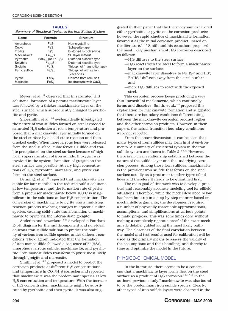
From the above discussion, it can be seen that many types of iron sulfides may form in H2S environ-ments. A summary of structural typism in the iron sulfide system are shown in Table 2.3-5,19 However, there is no clear relationship established between the nature of the sulfide layer and the underlying corro-sion process. Among those iron sulfides, mackinawite is the prevalent iron sulfide that forms on the steel surface usually as a precursor to other types of sul-fides and therefore it needs to be quantified first.

The main goal of this work was to develop a prac-tical and reasonably accurate modeling tool for oilfield situations. Therefore, while the model described below has been built up in a step-by-step manner based on mechanistic arguments, the development required a number of physically reasonable approximations, assumptions, and simplifications at various points to make progress. This was sometimes done without making a completely rigorous proof of the exact mech-anistic details, guided along the most likely path-way. The closeness of the final correlation between the model and test results used for calibration will be used as the primary means to assess the validity of the assumptions and their handling, and thereby to tune and optimize the model in the future.

PhysIco-chemIcAl model

In the literature, there seems to be a consen-sus that a mackinawite layer forms first on the steel surface as a product of H2S corrosion.1-5,17,19 In the authors’ previous study,9 mackinawite was also found to be the predominant iron sulfide species. Clearly, other types of iron sulfide layers were observed in the

TAble 2Summary of Structural Typism in the Iron Sulfide System

Name Formula Structure

Amorphous FeS Non-crystalline Cubic FeS Sphalerite-type Troilite FeS Distorted niccolite-type Mackinawite Fe1+xS 2D layer material Pyrrhotite FeS1+x (or Fe1−xS) Distorted niccolite-type Smythite Fe3+xS4 Distorted niccolite-type Greigite Fe3S4 Thiospinel (magnetite-type) Ferric sulfide Fe2S3 Thiospinel with cation vacancies Pyrite FeS2 Derived from rock salt Marcasite FeS2 Isostructural with CaCl2



past on the steel surfaces attacked by H2S, particu-larly in long exposures; however, it is still unclear what effect the variation in layer composition may have on the corrosion rate.

Based on an analogy with iron carbonate forma-tion in CO2 solutions8 and due to its rather low solu-bility, mackinawite was thought to form by a precipi-tation mechanism.20 While this is clearly a possibility, as argued above, mackinawite formation via a direct heterogeneous chemical reaction with iron on the steel surface seems to be the more plausible mecha-nism because of the following pieces of evidence:

—Due to the very high reactivity of H2S with iron, the mackinawite layer has been shown to form in minutes,1-2,21 which is much faster than what one would expect from the typical kinetics for a precipitation process.1

—Formation of a solid mackinawite layer is observed in highly undersaturated solutions1 (e.g., pH 3) where it is thermodynamically unstable. A case can be made that the reason-ing about solubility of iron sulfide based on conditions in the bulk is invalid, since at a steel surface, due to corrosion of iron, there always exists a higher pH and a possibility to exceed the mackinawite solubility limit, even in acidic solutions. This argument would apply to even lower pH as well as to other precipitating salts such as iron carbonate. In reality, macroscopic iron carbonate layers are not observed at pH significantly below the solubility limit22-24 (based on bulk conditions), while iron sulfide layers are.10 In addition, basing arguments on a sur-face pH, which is very difficult to measure, is less practical. A way to reconcile the two argu-ments is to assume that upon iron dissolution, the ferrous ions never get very “far” from the steel surface due to a high local pH and rapidly form iron sulfide by precipitation. When taken to the limit, this argument amounts to a direct reaction between iron and H2S.

—There is little effect of bulk solution supersatu-ration level on the rate of mackinawite forma-tion.20

—The layered structure of the mackinawite layer often contains cracks and delaminations, with the steel surface imprint visible even after rather long exposures20 (Figure 1).

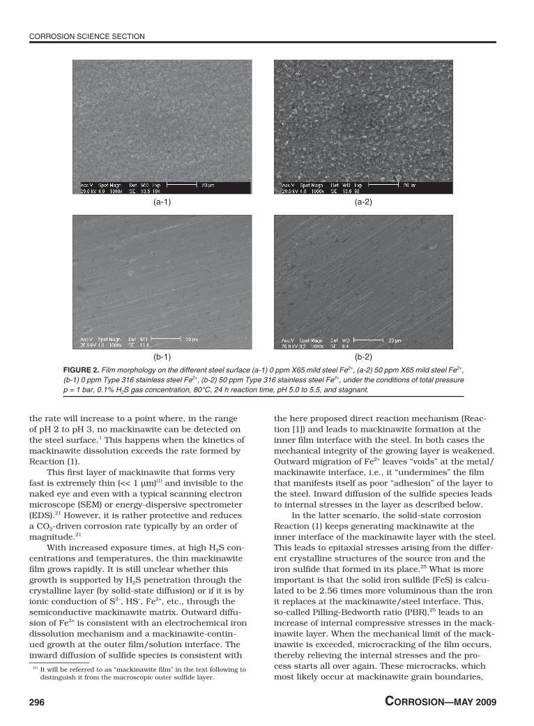
—The amount of mackinawite layer always being smaller than the amount of iron lost to corro-sion of mild steel (expressed in molar units)9 and a lack of substantial mackinawite layer for-mation on stainless steel and other corrosion-resistant alloys (Figure 2), both suggest that the iron “source” in mackinawite is the steel itself, rather than the bulk solution.

—Mackinawite layers in corrosion tests have very similar structures and morphologies as the

mackinawite layer seen in high-temperature sulfidation of mild steel exposed to gaseous or hydrocarbon environments,25-27 where the pre-cipitation mechanism is impossible.

If the list above is accepted as sufficient evidence, it can be concluded that the corrosion of mild steel in H2S aqueous environments proceeds initially by a very fast, direct, heterogeneous reaction at the steel sur-face to form a solid adherent mackinawite layer. The overall reaction scheme can be written as:

Fe(s) + H2S & FeS(s) + H2 (1)

Since the initial and final states of Fe are solid, this reaction is often referred to as the “solid-state corro-sion reaction.” The formed mackinawite layer may dis-solve depending on the solution saturation level. For the typical pH range seen in oilfield brines (pH 4 to 7), the solution is often supersaturated with respect to iron sulfide and the mackinawite layer does not dissolve. Actually, in long exposures, iron sulfide grows by precipitation from the bulk.28 If the pH is decreased below saturation the dissolution starts and

(a)

(b)

FIguRe 1. Film morphology showing polishing marks on the X65 mild steel, (a) 1,000X and (b) 5,000X, under the conditions of total pressure p = 1 bar, 0 ppm initial Fe2+ aqueous concentration, 10% H2S gas concentration, 60°C, 1 h reaction time, pH 5.0 to 5.5, and stagnant.



the rate will increase to a point where, in the range of pH 2 to pH 3, no mackinawite can be detected on the steel surface.1 This happens when the kinetics of mackinawite dissolution exceeds the rate formed by Reaction (1).

This first layer of mackinawite that forms very fast is extremely thin (<< 1 μm)(1) and invisible to the naked eye and even with a typical scanning electron microscope (SEM) or energy-dispersive spectrometer (EDS).21 However, it is rather protective and reduces a CO2-driven corrosion rate typically by an order of magnitude.21

With increased exposure times, at high H2S con-centrations and temperatures, the thin mackinawite film grows rapidly. It is still unclear whether this growth is supported by H2S penetration through the crystalline layer (by solid-state diffusion) or if it is by ionic conduction of S2–, HS–, Fe2+, etc., through the semiconductive mackinawite matrix. Outward diffu-sion of Fe2+ is consistent with an electrochemical iron dissolution mechanism and a mackinawite-contin-ued growth at the outer film/solution interface. The inward diffusion of sulfide species is consistent with

the here proposed direct reaction mechanism (Reac-tion [1]) and leads to mackinawite formation at the inner film interface with the steel. In both cases the mechanical integrity of the growing layer is weakened. Outward migration of Fe2+ leaves “voids” at the metal/mackinawite interface, i.e., it “undermines” the film that manifests itself as poor “adhesion” of the layer to the steel. Inward diffusion of the sulfide species leads to internal stresses in the layer as described below.

In the latter scenario, the solid-state corrosion Reaction (1) keeps generating mackinawite at the inner interface of the mackinawite layer with the steel. This leads to epitaxial stresses arising from the differ-ent crystalline structures of the source iron and the iron sulfide that formed in its place.25 What is more important is that the solid iron sulfide (FeS) is calcu-lated to be 2.56 times more voluminous than the iron it replaces at the mackinawite/steel interface. This, so-called Pilling-Bedworth ratio (PBR),25 leads to an increase of internal compressive stresses in the mack-inawite layer. When the mechanical limit of the mack-inawite is exceeded, microcracking of the film occurs, thereby relieving the internal stresses and the pro-cess starts all over again. These microcracks, which most likely occur at mackinawite grain boundaries,

(a-1)

(b-1)

(a-2)

(b-2)

FIguRe 2. Film morphology on the different steel surface (a-1) 0 ppm X65 mild steel Fe2+, (a-2) 50 ppm X65 mild steel Fe2+, (b-1) 0 ppm Type 316 stainless steel Fe2+, (b-2) 50 ppm Type 316 stainless steel Fe2+, under the conditions of total pressure p = 1 bar, 0.1% H2S gas concentration, 80°C, 24 h reaction time, pH 5.0 to 5.5, and stagnant.

(1) It will be referred to as “mackinawite film” in the text following to distinguish it from the macroscopic outer sulfide layer.



serve as preferred pathways for a more rapid penetra-tion of sulfide species, which fuel the solid-state Reac-tion (1) to go even faster.29 It is expected that in some instances, at stress concentration points, large cracks in the film may appear as shown in Figure 1, which is confirmed to be a mackinawite film by x-ray diffrac-tion (XRD).9 The sulfide species penetrate even more easily at these locations to fuel the corrosion Reac-tion (1), which makes even more sulfide film at those locations and causes even more internal stressing and film failure. It is not difficult to see how this “feed-for-ward” scenario could lead to an exponential growth of the reaction rate and localized corrosion in certain locations. This scenario also offers an explanation for an apparently odd occurrence in H2S corrosion: exper-imental observations indicate that pits are usually full of iron sulfide and even have a cap of sulfide, which is thicker than elsewhere on the steel surface, as shown in Figure 3 provided by Brown and Nesic.30 This appearance is very different from the localized attack seen in CO2 corrosion where pits are bare while the surrounding steel is covered with a protective layer. Finally, in this scenario the hydrogen atoms evolved by the corrosion Reaction (1) buildup at the steel/film interface because they can diffuse out through the tight mackinawite film only with some difficulty. This may lead to enhanced hydrogen penetration into the steel. On the other hand, the hydrogen built up at the steel/layer interface may build up pressure and “bubble out” and cause further damage to the mack-inawite layer. The last few points are purely specu-lative and are discussed here only because they are consistent with the proposed mechanism of H2S cor-rosion of steel and the resulting iron sulfide layer growth. As there is no direct evidence for them in the experiments presented in this work, these hypotheses require further evaluation in the future.

As the mackinawite layer goes through the growth/microcracking cycle, it thickens. As larger

cracks appear, whole portions of the layer may par-tially delaminate from the steel surface starting another cycle of rapid layer growth underneath, as shown in Figure 4. Over longer exposures, this cyclic growth/delamination process leads to a macroscopi-cally layered structure, which is rather porous. As this layer grows it will spontaneously spall, a process assisted by flow. If the bulk solution is undersaturated (typically at 3 < pH < 4), the outer porous mackinawite layer will dissolve. This may happen even to the very tight and thin inner mackinawite film at pH < 3.1

In summary, in H2S corrosion of mild steel, two types of mackinawite layers form on the steel surface:

—a very thin (<<1 μm) and tight inner film —a much thicker (>>1 μm) outer layer, which is

loose and very porousThe outer layer may be intermixed with any iron

sulfide or iron carbonate that may have precipitated, given the favorable water chemistry and long exposure

(a) (b)

FIguRe 3. (a) Morphology and (b) cross section of the localized attack on the X65 mild steel surface in CO2/H2S environment under the conditions of 8 bar Ptot, 8 mbar PH2S, 7.5 bar PCO2, 60°C, and the total reaction time is 10 days.30

FIguRe 4. Cross section of the layer formed on the X65 mild steel surface (at 1,000X) under the conditions of total pressure p = 1 bar, 0 ppm initial Fe2+ aqueous concentration, 10% H2S gas concentration (H2S/N2 gas), 80°C, pH 5, and 24-h total reaction time.



time, which would change its properties and appear-ance. Both the inner mackinawite layer and the outer layer act as barriers for the diffusion of the sulfide species, which fuel the solid-state corrosion Reac-tion (1). This is in addition to the diffusion resistance through the aqueous mass-transfer boundary layer. In the authors’ opinion, the hypothesis about outward diffusion by the Fe2+ through the thin mackinawite layer can be rejected since it is inconsistent with the proposed solid-state corrosion Reaction (1) and would lead to a formation of a very different looking and behaving sulfide layer in a process that is more akin to iron carbonate formation in CO2 corrosion.

When CO2 is present in the solution, both iron carbonate and iron sulfide may form on the steel sur-face, depending on the water chemistry as well as the competitiveness of iron carbonate and iron sulfide formation. Based on the previous investigation,9 it is

found that mackinawite layer formation is the domi-nant process in most cases of mixed CO2/H2S corro-sion. In some cases, iron carbonate crystals may form intermixed with the mackinawite layer (for an example see Figure 5 [experiment with 0.1% H2S, Fe2+ 50 ppm, and 80°C]), which was confirmed using XRD (Figure 6). However, the first mackinawite layer is assembled extremely quickly by a solid-state reaction; hence, it always forms first on the steel surface. The iron car-bonate crystals may precipitate in the outer part of the mackinawite layer according to the crystal mor-phology, as shown in Figure 5. Therefore, it is believed that in mixed CO2/H2S systems, the mackinawite layer still partially protects the steel from corrosion, and the description of the H2S corrosion process pre-sented above for pure H2S corrosion is also applica-ble for CO2/H2S corrosion, with small modifications. The assumptions that iron carbonate layer formation has little effect on the CO2/H2S corrosion process is a simplification; however, it does allow development of a practical working model.

mAthemAtIcAl model

H2S Corrosion Based on the experimental results and the

description of the H2S corrosion process presented above, a mathematical model can be constructed. The key assumptions are:

—the corrosion process happens via a direct het-erogeneous solid-state Reaction (1) at the steel surface;

—there is always a very thin (<<1 μm) but dense film of mackinawite at the steel surface, which acts as a solid-state diffusion barrier for the sulfide species involved in the corrosion reac-tion;

FIguRe 5. Morphology of layer formed on the X65 mild steel surface under the conditions of 0.1% H2S (H2S/CO2 gas), 80°C, pH 6.5 ~ 6.6, Fe2+ = 50 ppm, and 24-h total reaction time.

FIguRe 6. XRD results of layer formed on the X65 mild steel surface under the conditions of 0.1% H2S (H2S/CO2 gas), 80°C, pH 6.5 ~ 6.6, Fe2+ = 50 ppm, and 24-h total reaction time.



—this fi lm continuously goes through a cyclic process of growth, cracking, and delamination, which generates the outer mackinawite layer;

—this outer layer grows in thickness (typically >1 μm) over time and presents a diffusion barrier;

—the outer layer is very porous and rather loosely attached; over time it cracks, peels, and spalls, a process aggravated by the fl ow.

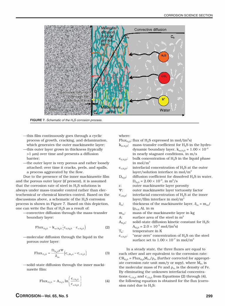
Due to the presence of the inner mackinawite fi lm and the porous outer layer (if present), it is assumed that the corrosion rate of steel in H2S solutions is always under mass-transfer control rather than elec-trochemical or chemical kinetics control. Based on the discussions above, a schematic of the H2S corrosion process is shown in Figure 7. Based on this depiction, one can write the fl ux of H2S as a result of:

—convective diffusion through the mass-transfer boundary layer:

Flux k cH S k cm Hk cS bk cS bk c2 2

k c2 2

k cH S2 2H S m H2 2m Hk cm Hk c2 2

k cm Hk c= ( )k c( )k c c( )cS b( )S bk cS bk c( )k cS bk c H S( )H S o H( )o H S( )S2 2( )2 2c

2 2c( )c

2 2cH S2 2H S( )H S2 2H S o H2 2o H( )o H2 2o H, ,S b, ,S b2 2, ,2 2m H2 2m H, ,m H2 2m H ( ), ,( )S b( )S b, ,S b( )S b 2 2( )2 2,2 2( )2 2o H2 2o H( )o H2 2o H,o H2 2o H( )o H2 2o H( )–( ) (2)

—molecular diffusion through the liquid in the porous outer layer:

Flux

DH S

H S

os2H S2H S

2H S2H S= ( )c c( )c co H( )o Hc co Hc c( )c co Hc cS i( )S ic cS ic c( )c cS ic c H S( )H S2 2( )2 2c c

2 2c c( )c c

2 2c cS i2 2S i( )S i2 2S ic cS ic c

2 2c cS ic c( )c cS ic c

2 2c cS ic c H S2 2H S( )H S2 2H S

εδ

Ψ ( ), ,( )o H( )o H, ,o H( )o H2 2( )2 2, ,2 2( )2 2S i2 2S i( )S i2 2S i, ,S i2 2S i( )S i2 2S ic c( )c c–c c( )c c

(3)

—solid-state diffusion through the inner macki-nawite fi lm:

Flux A

c

cH S H S

i H S

s H S2 2H S2 2H S H S2 2H S

2

2

=

ln ,i H,i H

,s H,s H (4)

where:FluxH2S: fl ux of H2S expressed in mol/(m2s)km,H2S: mass-transfer coeffi cient for H2S in the hydro-

dynamic boundary layer, km,H2S = 1.00 × 10–4 in nearly stagnant conditions, in m/s

cb,H2S: bulk concentration of H2S in the liquid phase in mol/m3

co,H2S: interfacial concentration of H2S at the outer layer/solution interface in mol/m3

DH2S: diffusion coeffi cient for dissolved H2S in water, DH2S = 2.00 × 10–9, in m2/s

ε: outer mackinawite layer porosityΨ: outer mackinawite layer tortuosity factorci,H2S: interfacial concentration of H2S at the inner

layer/fi lm interface in mol/m3

δos: thickness of the mackinawite layer, δos = mos/(ρFeS A), in m

mos: mass of the mackinawite layer in kgA: surface area of the steel in m2

AH2S: solid-state diffusion kinetic constant for H2S: AH2S = 2.0 × 10–5 mol/(m2s)

Tk: temperature in Kcs,H2S: “near-zero” concentration of H2S on the steel

surface set to 1.00 × 10–7 in mol/m3

In a steady state, the three fl uxes are equal to each other and are equivalent to the corrosion rate: CRH2S = FluxH2SMFe/ρFe (further corrected for appropri-ate corrosion rate unit mm/y or mpy), where MFe is the molecular mass of Fe and ρFe is the density of Fe. By eliminating the unknown interfacial concentra-tions co,H2S and ci,H2S from Equations (2) through (4), the following equation is obtained for the fl ux (corro-sion rate) due to H2S:

FIguRe 7. Schematic of the H2S corrosion process.



Flux A

c FluxD k

H S H S

b Hc Fb Hc FS Hc FS Hc FluS HluxS Hx SH SD kH SD km

2 2H S2 2H S H S2 2H S

2 2c F

2 2c FS H2 2S Hc FS Hc F

2 2c FS Hc FluS Hlu

2 2luS Hlu

2H S2H S

0 5 1

=

+

ln

c F–c F,b H,b H0 5.0 5

,

δεΨD kεΨD k H SHH SH

s H Sc2H S2H S

2

,s H,s H (5)

This is an algebraic, nonlinear equation with respect to FluxH2S, which does not have an explicit solution but can be solved by using a simple, numerical algo-rithm such as the interval halving method or simi-lar. These are available as ready-made routines in spreadsheet applications or in any common computer programming language. The prediction for FluxH2S depends on a number of constants used in the model that can be found in handbooks (such as DH2S), calcu-lated from the established theory (e.g., km,H2S), or are determined from experiments (e.g., AH2S, cs,H2S). The unknown thickness of the outer sulfi de layer changes with time and needs to be calculated as described below.

It is assumed that the amount of layer retained on the metal surface at any point in time depends on the balance of:

—layer formation kinetics (because the layer is generated by spalling of the thin mackinawite fi lm underneath it and by precipitation from the solution), and

—layer damage kinetics (because the layer is damaged by intrinsic or hydrodynamic stresses and/or by chemical dissolution).

SRR = SFR – SDR sulfi de layer sulfi de layer sulfi de layer retention formation damage rate rate rate

} } }

(6)

where all the terms are expressed in mol/(m2s). It is assumed here that in the typical range of application (4 < pH < 7), precipitation and dissolution of the iron sulfi de layer do not play a signifi cant role, so it can be written:

SRR = CR – SDRm SRR = CR – SDRm SRR = CR – SDR

sulfi de layer corrosion sulfi de layer retention rate mechanical rate damage rate

} } }

(7)

Experiments9 have shown that even in stagnant con-ditions about half of the sulfi de layer that forms is lost from the steel surface due to intrinsic growth stresses by internal cracking and spalling, i.e.:

SDRm ≈ 0.5 CR (8)

More experimentation is required to determine how the mechanical layer damage is affected by hydrody-namic forces.

Once the layer retention rate SRR is known, the change in mass of the outer sulfi de layer can easily be calculated as:

∆mos = SRR MFeS A ∆t (9)

where MFeS is the molar mass of iron sulfi de in kg/mol and ∆t is the time interval in seconds. The porosity of the outer mackinawite layer was determined to be very high (ε ≈ 0.9) by comparing the weight of the layer with the cross-sectional SEM images showing its thickness. On the other hand, this layer has proven to be rather protective (i.e., impermeable to diffusion), which can only be explained by its low tortuosity aris-ing from its layered structure. By matching the mea-sured and calculated corrosion rates in the presence of the outer mackinawite layer, the tortuosity factor was calculated to be Ψ = 0.003.

A time-marching explicit solution procedure could now be established where:

—the corrosion rate FluxH2S in the absence of the outer sulfi de layer can be calculated by using Equation (5), and assuming δos = 0;

—the amount of sulfi de layer ∆mos formed over a time interval ∆t is calculated by using Equation (9);

—the new corrosion rate FluxH2S in the presence of the sulfi de layer can be recalculated by using Equation (5);

—a new time interval ∆t is set and the second and third steps are repeated.

Effect of pHA small complication arises from the fact that at

very low H2S gas concentrations (ppmw range), there is very little dissolved H2S and the corrosion rate is directly affected by pH. A mackinawite layer still forms and controls the corrosion rate; however, the corro-sion process is largely driven by the reduction of pro-tons, rather than of H2S (the case shown in Reaction [1]). In an analogy with the approach laid out above, the convective diffusion fl ux of protons through the mass-transfer boundary layer is:

Flux k cH m H b

k cH b

k c+ +k c+ +k cH m+ +H m H b+ +H b

k cH b

k c+ +k cH b

k c=+ +=+ + ( )k c( )k c c( )cH b( )H b

k cH b

k c( )k cH b

k cH o( )H o H( )H+ +( )+ +c+ +c( )c+ +cH o+ +H o( )H o+ +H o H+ +H( )H+ +H, ,H b, ,H b( ), ,( )H b( )H b, ,H b( )H b( ),( )( )–( ) (10)

which in a steady state is equal to the diffusion fl ux of protons through the pores of the iron sulfi de layer:

Flux

DH

H

oc+

+= ( )c c( )c co H( )o H i H( )i H+ +( )+ +c c+ +c c( )c c+ +c c

i H+ +i H( )i H+ +i H

εδ

Ψ ( ), ,( )o H( )o H, ,o H( )o H i H( )i H, ,i H( )i Hc c( )c c–c c( )c c

(11)

which is equal to the solid-state diffusion fl ux of pro-tons through the thin mackinawite fi lm:

Flux A

c

cH H

i H

s H

+ +A+ +AH H+ +H H

+

+

=+ +=+ +

ln ,i H,i H

,s H,s H (12)

which is equivalent to the corrosion rate by protons: CRH+ = Flux MH Fe

Fe

+

2 ρ (further corrected for the appropriate corrosion rate unit).



By eliminating the unknown interfacial concen-trations co,H+ and ci,H+ from Equations (10) through (12), the following expression is obtained for the fl ux of protons controlled by the presence of the iron sul-fi de layers:

FluxH + = AH + ln cs,H +

cb,H + - FluxH +

DH +εΨ

δ0.5+

km,H +

1e o

(13)

where:FluxH+: fl ux of protons expressed in mol/(m2s)km,H+: mass-transfer coeffi cient for protons in the

hydrodynamic boundary layer, km,H+ = 3.00 × 10–4 in nearly stagnant condition, in m/s

cb,H+: bulk concentration of H+ in the liquid phase in mol/m3

co,H+: interfacial concentration of H+ at the outer layer/solution interface in mol/m3

DH+: diffusion coeffi cient for dissolved H+ in water, DH+ = 2.80 × 10–8, in m2/s

ci,H+: interfacial concentration of H+ at the inner layer/fi lm interface in mol/m3

AH+: solid-state diffusion kinetic constant for H+: AH+ = 4.0 × 10–4 mol/(m2s)

cs,H+: “near-zero” concentration of H+ on the steel surface set to 1.00 × 10–7 in mol/m3

The total rate of corrosion in this case is equal to the sum of the corrosion caused by H2S and the corro-sion caused by H+:

Cr CR CRH S H= +CR= +CRH S= +H S +2H S2H SH S= +H S2H S= +H S (14)

This description completes the explanation of a basic mechanistic model of pure H2S corrosion of mild steel. Based on the present model, a similar expres-sion is proposed for combined CO2/H2S corrosion below.

Effect of CO2

In the case of mixed H2S/CO2 corrosion, the mass-transfer-limited fl ux of CO2 can be calculated from the:—convective diffusion of CO2 through the mass-trans-

fer boundary layer:

Flux k cCO k cm Ck cO bk cO bk c2 2k c2 2k cm C2 2m Ck cm Ck c2 2k cm Ck cO b2 2O bk cO bk c2 2k cO bk c= ( )k c( )k c c( )cO b( )O bk cO bk c( )k cO bk c CO( )CO o C( )o CO( )O2 2( )2 2c2 2c( )c2 2co C2 2o C( )o C2 2o CO2 2O( )O2 2O, ,O b, ,O b2 2, ,2 2m C2 2m C, ,m C2 2m CO b2 2O b, ,O b2 2O b( ), ,( )O b( )O b, ,O b( )O b 2 2( )2 2,2 2( )2 2o C2 2o C( )o C2 2o C,o C2 2o C( )o C2 2o C( )–( ) (15)

—molecular diffusion of CO2 through the liquid in the porous outer sulfi de layer:

Flux

DCO

CO2

2

0 5

= ( )c c( )c co C( )o Cc co Cc c( )c co Cc cO i( )O ic cO ic c( )c cO ic c CO( )CO2 2( )2 2O i2 2O i( )O i2 2O ic cO ic c2 2c cO ic c( )c cO ic c2 2c cO ic c CO2 2CO( )CO2 2CO

εδ

Ψ0 5.0 5

( ), ,( )o C( )o C, ,o C( )o CO i( )O i, ,O i( )O i2 2( )2 2, ,2 2( )2 2O i2 2O i( )O i2 2O i, ,O i2 2O i( )O i2 2O ic c( )c c–c c( )c cc cO ic c( )c cO ic c–c cO ic c( )c cO ic c

(16)

—solid-state diffusion of CO2 through the inner mack-inawite fi lm:

Flux A

cc

CO COi CO

s CO2 2A2 2ACO2 2CO

2

2

=

ln ,i C,i C

,s C,s C (17)

which is equivalent to the corrosion rate by CO2: CRCO2

= FluxCO2 MFe/ρFe (further corrected for appropriate

corrosion rate unit).By eliminating the unknown interfacial concen-

trations co,CO2 and ci,CO2

, from Equations (15) through (17), the following expression is obtained for the corro-sion rate driven by the presence of CO2 and controlled by the presence of the iron sulfi de layers:

Flux A

c FluxD k

CO CO

b Cc Fb Cc FO Cc FO Cc FluO CluxO Cx OCOD kCOD km

2 2CO2 2CO

2 2O C2 2O Cc FO Cc F2 2

c FO Cc FluO Clu2 2

luO Clu O2 2O

2

0 5 1

=

+

ln

c F–c F,b C,b C0 5.0 5

,

δεΨD kεΨD k COCCOC

s COc2

2

,s C,s C (18)

where:FluxCO2

: fl ux of CO2 expressed in mol/(m2s)km,CO2

: mass-transfer coeffi cient for CO2 in the hydro-dynamic boundary layer, km,CO2

= 1.00 × 10–4 in nearly stagnant conditions, in m/s

cb,CO2: bulk concentration of CO2 in the liquid phase

in mol/m3

co,CO2: interfacial concentration of CO2 at the outer

layer/solution interface in mol/m3

DCO2: diffusion coeffi cient for dissolved CO2 in

water, DCO2 = 1.96 × 10–9, in m2/s

ci,CO2: interfacial concentration of CO2 at the inner

layer/fi lm interface in mol/m3

ACO2: solid-state diffusion kinetic constant for CO

2:

ACO2 = 2.0 × 10–6 mol/(m2s)

cs,CO2: concentration of CO2 on the steel surface in

mol/m3

In the H2S corrosion model presented above, pure mass-transfer control is assumed, and hence, the cs,H2S and cs,H+ are set to be virtually zero (practi-cally a very small value of 1.00 × 10–7 mol/m3). In CO2 corrosion, it is the carbonic acid (H2CO3) that is the corrosive species, and one must account for the fact that the CO2 hydration step-forming H2CO3 at the steel surface is a slow rate-controlling process. Therefore, the CO2 fl ux can be equated to the limit ing rate of H2CO3 hydration at the steel surface as fol-lows:31

Flux c DCO c Ds Cc DO Hc DO Hc D2 2c D2 2c Ds C2 2s Cc Ds Cc D2 2c Ds Cc DO H2 2O Hc DO Hc D2 2c DO Hc D0 5

= ( )c D( )c D k K( )k KO H( )O Hc DO Hc D( )c DO Hc D CO( )CO hy( )hyk Khyk K( )k Khyk Kd( )dk Kdk K( )k Kdk Kf( )fk Kfk K( )k Kfk Khy( )hyd( )d2 3( )2 3CO2 3CO( )CO2 3CO2 2,2 2s C2 2s C,s C2 2s C

0 5.0 5( )εΨ( ) (19)

where:DH2CO3

: diffusion coeffi cient of H2CO3 in m2/sKhyd: equilibrium constant for the CO2 hydration

reactionkf

hyd: forward reaction rate for the CO2 hydration reaction

By eliminating cs,CO2 from Equations (18) and (19),

the CO2 fl ux equation takes its fi nal form:



Flux A

c FluxD k

CO CO

b Cc Fb Cc FO Cc FO Cc FluO CluxO Cx OCOD kCOD km

2 2CO2 2CO

2 2O C2 2O Cc FO Cc F2 2

c FO Cc FluO Clu2 2

luO Clu O2 2O

2

0 5 1

=

+

ln

c F–c F,b C,b C0 5.0 5

,

δεΨD kεΨD k COCCOC

COFlux2

2

( )H C( )H CO h( )O hyd( )ydf( )f

hy( )hyd( )dD k( )D kH CD kH C( )H CD kH CO hD kO h( )O hD kO h K( )K2 3( )2 3H C2 3H C( )H C2 3H CO h2 3O h( )O h2 3O hO h( )O hεΨO h( )O hD k( )D kεΨD k( )D kO hD kO h( )O hD kO hεΨO hD kO h( )O hD kO h

(20)

The bulk concentration of CO2, cb,CO2, can be obtained

via Henry’s law:

c P Kb Cc Pb Cc PO Cc PO Cc P O sKO sK ol,b C,b C 2 2O C2 2O Cc PO Cc P2 2c PO Cc P O s2 2O s= ×c P= ×c PO C= ×O Cc PO Cc P= ×c PO Cc P O s= ×O s2 2= ×2 2O C2 2O C= ×O C2 2O Cc PO Cc P2 2c PO Cc P= ×c PO Cc P2 2c PO Cc P O s2 2O s= ×O s2 2O s (21)

where Henry’s constant is a function of temperature and ionic strength:

Ksol = ×= ×14 5

1 0025810

..

– .( )T( )Tf( )fTfT( )TfT+ ×( )+ ×2 2( )2 27 5( )7 5+ ×7 5+ ×( )+ ×7 5+ ×65( )65+ ×65+ ×( )+ ×65+ ×65( )65 10( )10 8 0( )8 06 1( )6 1×6 1×( )×6 1×3( )3– .( )– .2 2– .2 2( )2 2– .2 2 . –( ). –T. –T( )T. –Tf. –f( )f. –fTfT. –TfT( )TfT. –TfT. –( ). –+ ×. –+ ×( )+ ×. –+ ×. –( ). –+ ×. –+ ×( )+ ×. –+ ×65. –65( )65. –65+ ×65+ ×. –+ ×65+ ×( )+ ×65+ ×. –+ ×65+ ×10. –10( )10. –10 8 0.8 0( )8 0.8 0–( )– 0 0( )0 000 00( )00 00 075( )0756 2( )6 20 06 20 0( )0 06 20 0–( )–0 0–0 0( )0 0–0 0.( ).T I( )T I0 0T I0 0( )0 0T I0 0 075T I075( )075T I0750 06 20 0T I0 06 20 0( )0 06 20 0T I0 06 20 0f( )f0 0f0 0( )0 0f0 00 0T I0 0f0 0T I0 0( )0 0T I0 0f0 0T I0 0T I+ ×T I( )T I+ ×T I0 0T I0 0+ ×0 0T I0 0( )0 0T I0 0+ ×0 0T I0 0 075T I075+ ×075T I075( )075T I075+ ×075T I075.T I.+ ×.T I.( ).T I.+ ×.T I.

(22)32

Tf is the temperature in °F and I is the ionic strength in mol/L.

By solving the above equation, the CO2 corrosion rate can be obtained and introduced into Equation (23) below to obtain the total corrosion rate in mixed CO2/H2S environments:

CR CR CR CRH S H CO= +CR= +CRH S= +H S ++2 2CR2 2CR CR2 2CRH S2 2H S H2 2H CO2 2CO= +2 2= +H S= +H S2 2H S= +H S +2 2++2 2+ (23)

For the corrosion rates caused by H2S and H+, the same expressions can be used as presented above for a CO2-free environment, Equations (5) and (13), respectively.

VerIfIcAtIon And testIng of the model

Experiments by Sun33

To formulate the model and calibrate its perfor-mance, the experimental fi ndings of Sun33 were used as the primary source. Figure 8 shows the comparison

of the corrosion rate vs. the reaction time for a series of pure H2S experiments (pH2S = 0.5 mbar to 50 mbar) done at pH 5 and 80°C, conducted by Sun.33 Clearly, the model successfully captures the rapid reduction of the corrosion rate with time due to the growth of an iron sulfi de layer. While an attempt was made to cap-ture the very short-term data (obtained after 1 h of exposure), this was not always accurate and the main effort was directed to predicting the 24-h data points accurately. From Figure 8, one can observe that H2S partial pressure plays an important role in corrosion. At pH2S = 50 mbar, H2S is the main corrosive species (contributing 98% to the overall corrosion damage when compared to only 2% attributed to H+). When the amount of H2S is reduced 100 times (pH2S = 0.5 mbar), both species are responsible for approxi-mately one half of the observed corrosion rate. Figure 9 shows the comparison of the measured and pre-dicted amount of iron sulfi de, which is retained on the steel surface at different reaction times. The pre-dicted layer growth is very rapid in the fi rst few hours and then gradually levels off, leading to what is often referred to as a “parabolic fi lm growth regime.”

Data were also collected by Sun33 under rather similar conditions, with the main difference being a higher pH 6.6 and the presence of CO2. The compari-son between measured and predicted corrosion rate in this mixed H2S/CO2 corrosion environment is shown in Figure 10. Very similar trends are observed with time at different pH2S, as was the case for a pure H2S environment. Upon closer inspection of the predic-tions, it is found that at a pCO2/pH2S ratio of 103 in the gas phase (pCO2 = 0.54 bar, pH2S = 0.54 mbar), the main corrosive species is CO2 (i.e., H2CO3) as expected, which is responsible for more than 90% of the corrosion rate. However, under these conditions the corrosion rate is still controlled by the presence of H2S, i.e., sulfi de layer, which reduces the pure CO2 (H2S-free) corrosion rate by more than 10 times. When the pCO2/pH2S ratio in the gas is reduced to 10, both corrosive gases contribute approximately the same to the overall corrosion rate.

The model was tested further by making simu-lations outside the range of parameters used to cali-brate it (taken from the experimental study of Sun33 mentioned above); i.e., the model was used to extrap-olate the corrosion rates to much lower and much higher partial pressures of H2S as well as much longer exposure times.

Experiments by Singer, et al.34

A similar range of H2S partial pressures, as reported by Sun,33 was investigated by Singer, et al.34 The key difference was the higher partial pressure of CO2 (pCO2 = 2 bar) and more importantly the long duration of experiments (21 days) conducted in strati-fi ed gas-liquid pipe fl ow. The comparison of the model predictions and the experimental results is given in

FIguRe 8. Corrosion rate vs. time; experimental data = points, model predictions = lines; conditions: total pressure p = 1 bar, H2S gas partial pressure from 0.54 mbar to 54 mbar, 80°C, experiment duration 1 h to 24 h, pH 5.0 to 5.5, stagnant. Experimental data taken from Sun.33



Figure 11, showing a marked decrease of pure CO2 corrosion rate due to the presence of H2S and a rea-sonable prediction made by the model particularly at longer exposure times. This is clearly a mixed CO2/H2S corrosion scenario. At a pCO2/pH2S ratio of 200 (pCO2 = 2 bar, pH2S = 4 mbar), the CO2 contribution to the corrosion rate is 75%, with most of the balance provided by H2S. At the pCO2/pH2S ratio of 28 (pCO2 = 2 bar, pH2S = 70 mbar), both CO2 and H2S account for approximately 50% of the overall corrosion rate.

Experiments by Smith and Pacheco5

Another study covering the same H2S partial pressure range was published by Smith and Pacheco.5 Three-day-long autoclave experiments were conducted at a very high total pressure (p = 138 bar) and a high CO2 partial pressure (pCO2 = 13.8 bar). When com-paring the predictions with the experimental results of Smith and Pacheco5 (Figure 12), it can be seen that the model underpredicts the observed rate of steel

FIguRe 9. Scale retention amount vs. time; experimental data = points, model predictions = lines; conditions: total pressure p = 1 bar, H2S gas partial pressure from 0.54 mbar to 54 mbar, 80°C, experiment duration 1 h to 24 h, pH 5.0 to 5.5, stagnant. Experimental data taken from Sun.33

FIguRe 10. Corrosion rate vs. time; experimental data = points, model predictions = lines; conditions: total pressure p = 1 bar, CO2 partial pressure 0.54 bar, H2S gas partial pressure from 0.54 mbar to 54 mbar, 80°C, experiment duration 1 h to 24 h, pH 6.6, stagnant. Experimental data taken from Sun.33

FIguRe 11. Corrosion rate vs. time; experimental data = points, model predictions = lines; conditions: total pressure p = 3 bar, CO2 partial pressure 2 bar, H2S gas partial pressure from 3 mbar to 70 mbar, 70°C, experiment duration 2 days through 21 days, pH 4.2 to 4.9, liquid velocity 0.3 m/s. Experimental data taken from Singer, et al.34

FIguRe 12. Corrosion rate vs. H2S partial pressure; experimental data = points, model predictions = lines; conditions: total pressure p = 137.9 bar, CO2 partial pressure 13.8 bar, H2S gas partial pressure from 40 mbar to 120 mbar, 50°C, experiment duration 3 days, pH 4.0 to 6.2, stagnant. Experimental data taken from Smith and Pacheco.5



corrosion by approximately a factor of two. However, when this is compared with a pure CO2 (H2S-free) cor-rosion rate under the same conditions (which is not reported but can be predicted at almost 20 mm/y), the accuracy of the model can be considered as rea-sonable. At the highest pCO2/pH2S ratio of 3,500 (pCO2 = 13.8 bar, pH2S = 40 mbar) tested by Smith and Pacheco,5 CO2 accounts for approximately 70% of the corrosion rate and 30% can be ascribed to H2S. At the lowest pCO2/pH2S ratio of 1,180 (pCO2 = 13.8 bar, pH2S = 116 mbar), CO2 accounts for approximately 57% of the corrosion rate and 43% can be ascribed to H2S.

Experiments by Lee10

An example of model performance at extremely low H2S partial pressures is seen in Figure 13, where

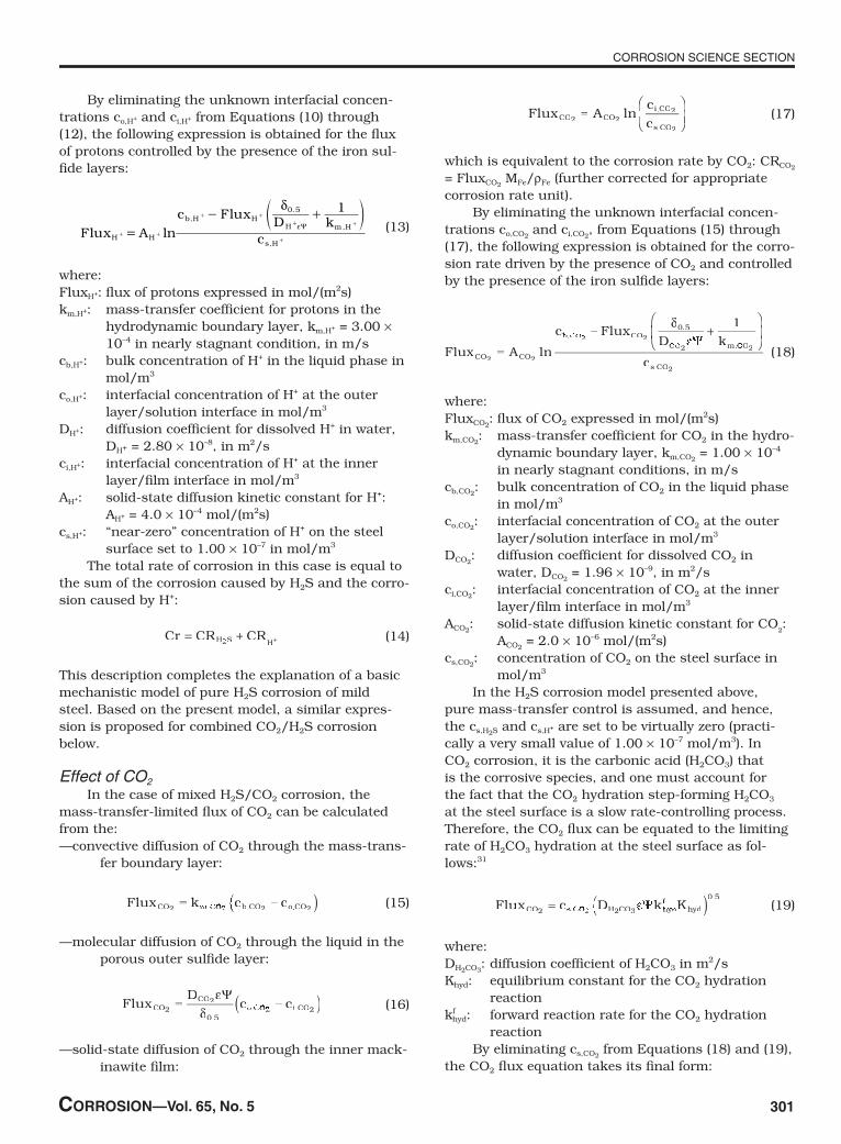
in the experiments conducted by Lee,10 pH2S ranged from 0.0013 mbar to 0.32 mbar, corresponding to 1 ppmm to 250 ppmm in the gas phase at 1 bar CO2. Clearly, this is a CO2-dominated corrosion scenario (pCO2/pH2S ratio is in the range from 103 to 106); however, again, the H2S controls the corrosion rate. Even when present in such minute amounts, H2S reduced the pure CO2 (H2S-free) corrosion rate by 3 to 10 times due to formation of a thin mackinawite film. The present model successfully captures this effect, as shown in Figure 13.

Experiments by Kvarekvål, et al.35

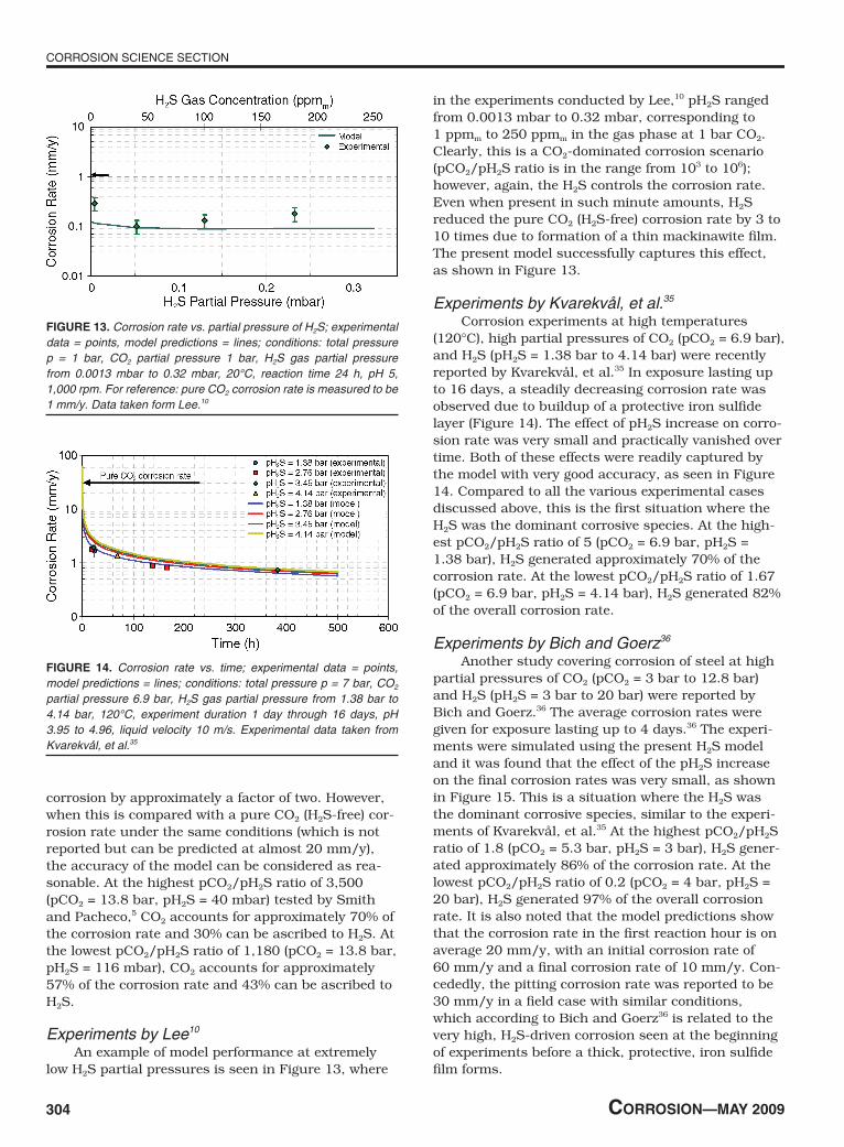
Corrosion experiments at high temperatures (120°C), high partial pressures of CO2 (pCO2 = 6.9 bar), and H2S (pH2S = 1.38 bar to 4.14 bar) were recently reported by Kvarekvål, et al.35 In exposure lasting up to 16 days, a steadily decreasing corrosion rate was observed due to buildup of a protective iron sulfide layer (Figure 14). The effect of pH2S increase on corro-sion rate was very small and practically vanished over time. Both of these effects were readily captured by the model with very good accuracy, as seen in Figure 14. Compared to all the various experimental cases discussed above, this is the first situation where the H2S was the dominant corrosive species. At the high-est pCO2/pH2S ratio of 5 (pCO2 = 6.9 bar, pH2S = 1.38 bar), H2S generated approximately 70% of the corrosion rate. At the lowest pCO2/pH2S ratio of 1.67 (pCO2 = 6.9 bar, pH2S = 4.14 bar), H2S generated 82% of the overall corrosion rate.

Experiments by Bich and Goerz36

Another study covering corrosion of steel at high partial pressures of CO2 (pCO2 = 3 bar to 12.8 bar) and H2S (pH2S = 3 bar to 20 bar) were reported by Bich and Goerz.36 The average corrosion rates were given for exposure lasting up to 4 days.36 The experi-ments were simulated using the present H2S model and it was found that the effect of the pH2S increase on the final corrosion rates was very small, as shown in Figure 15. This is a situation where the H2S was the dominant corrosive species, similar to the experi-ments of Kvarekvål, et al.35 At the highest pCO2/pH2S ratio of 1.8 (pCO2 = 5.3 bar, pH2S = 3 bar), H2S gener-ated approximately 86% of the corrosion rate. At the lowest pCO2/pH2S ratio of 0.2 (pCO2 = 4 bar, pH2S = 20 bar), H2S generated 97% of the overall corrosion rate. It is also noted that the model predictions show that the corrosion rate in the first reaction hour is on average 20 mm/y, with an initial corrosion rate of 60 mm/y and a final corrosion rate of 10 mm/y. Con-cededly, the pitting corrosion rate was reported to be 30 mm/y in a field case with similar conditions, which according to Bich and Goerz36 is related to the very high, H2S-driven corrosion seen at the beginning of experiments before a thick, protective, iron sulfide film forms.

FIguRe 13. Corrosion rate vs. partial pressure of H2S; experimental data = points, model predictions = lines; conditions: total pressure p = 1 bar, CO2 partial pressure 1 bar, H2S gas partial pressure from 0.0013 mbar to 0.32 mbar, 20°C, reaction time 24 h, pH 5, 1,000 rpm. For reference: pure CO2 corrosion rate is measured to be 1 mm/y. Data taken form Lee.10

FIguRe 14. Corrosion rate vs. time; experimental data = points, model predictions = lines; conditions: total pressure p = 7 bar, CO2 partial pressure 6.9 bar, H2S gas partial pressure from 1.38 bar to 4.14 bar, 120°C, experiment duration 1 day through 16 days, pH 3.95 to 4.96, liquid velocity 10 m/s. Experimental data taken from Kvarekvål, et al.35



Experiments by Omar, et al.37

H2S corrosion data collected at the most severe experimental conditions were published recently by Omar, et al.37 Long-term flow loop experiments (15 days to 21 days) were conducted at high partial pressure of H2S (pH2S = 10 bar to 30 bar), high partial pressure of CO2 (pCO2 = 3.3 bar to 10 bar), and low pH (2.9 to 3.2). The measured corrosion rates as a function of velocity are shown in Figure 16 for the three long-term experiments. No effect of velocity on the uniform corrosion rate could be observed in these long-term exposures, which is due to buildup of a thick, protective, sulfide layer. The model predictions also shown in Figure 16 confirm this trend and show a remarkable agreement with the experimental results in the less-extreme experiments 1 and 2 (pCO2 = 3.3 bar; pH2S = 10 bar), both at low (25°C) and high temperatures (80°C). In experiment no. 3, which was conducted at the most extreme set of conditions (pCO2 = 10 bar; pH2S = 30 bar) and high temperature (80°C), the model underpredicts the corrosion rate by a factor of 2.5. This brings us to the limitations of the model, which are discussed in the following section. In all three experiments reported by Omar, et al.,37 the pCO2/pH2S ratio was about 0.3; i.e., the corrosion process and corrosion rate were dominated completely by H2S, which contributed ≈95% of the corrosion rate.

lImItAtIons of the model And future work

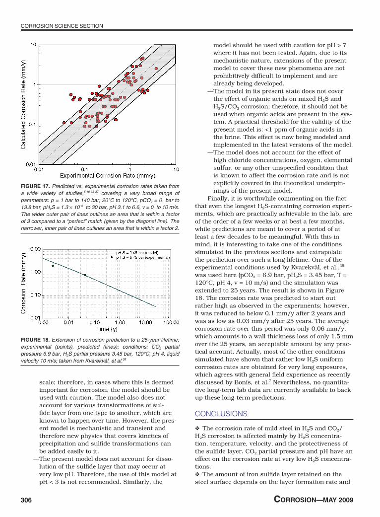
From the numerous comparisons made in the previous section, it is clear that the present mechanis-tic model of pure H2S and mixed H2S/CO2 corrosion has performed rather well over a very broad range of conditions. The summary of all the key experimental conditions as well as the resulting experimental and predicted corrosion rates are presented in Table 1. Actually, the partial pressure of H2S varies by 7 orders of magnitude, yet the predictions were typically within the conventional margin of error of the measurements and deviated by a factor not more than 2 to 3.(2) This is illustrated in Figure 17 where all the data (shown in Table 1) are presented in a parity plot in which the measured corrosion rates are compared directly with the predicted ones.

Nevertheless, the limitations of the present model need to be pointed out here, to avoid its misuse and to indicate the aspects open to improvement.

—The present model covers uniform H2S and H2S/CO2 corrosion. It does not predict localized

corrosion in either environment, neither does it cover pure CO2 corrosion (H2S-free condition). Making a link to an existing mechanistic elec-trochemical model of CO2 corrosion should not be difficult. Furthermore, the present model can be considered as a solid platform for construct-ing an H2S-driven localized corrosion model.

—While the present corrosion model covers a very broad range of H2S partial pressures, it is not recommended to use this model below pH2S = 0.01 mbar or above pH2S = 10 bar. Similar lim-its apply to the CO2 partial pressure. This leaves a very broad area of applicability for the present model.

—This model does not account for any precipita-tion of iron sulfide, iron carbonate, or any other

(2) When interpreting graphs such as the one shown in Figure 17, one should keep in mind that the various experimental data points always have a measurement error associated with them (not shown in Figure 17 for clarity reasons); i.e., the data collected in various experiments are not in perfect agreement with each other. Therefore, one has to account for this when comparing the experimental data with numerical predictions, which carry their own uncertainty (also not shown in Figure 17).

FIguRe 15. Corrosion rate vs. time; experimental data = points, model predictions = lines; Tests A and B: p = 8.3 bar, pCO2 = 5.3 bar, pH2S = 3 bar, 60°C, (A) 71 h and (B) 91 h; Test C: p = 24 bar, pCO2 = 4 bar, pH2S = 20 bar, 70°C, 91 h; Test D: p = 15.7 bar, pCO2 = 3.5 bar, pH2S = 12.2 bar, 65°C, 69 h; Test E: p = 20.8 bar, pCO2 = 12.8 bar, pH2S = 8 bar, 65°C, 91 h; Test F: p = 7.2 bar, pCO2 = 3 bar, pH2S = 4.2 bar, 65°C, 63 h; experimental data taken from Bich and Goerz.36

FIguRe 16. Corrosion rate vs. velocity; experimental data = points, model predictions = lines; Exp. 1.: 19 days, p = 40 bar, pCO2 = 3.3 bar, pH2S = 10 bar, 80°C, pH 3.1, v = 1 m/s to 5 m/s; Exp. 2.: 21 days, p = 40 bar, pCO2 = 3.3 bar, pH2S = 10 bar, 25°C, pH 3.2, v = 1 m/s to 5 m/s; Exp. 3.: 10 days, p = 40 bar, pCO2 = 10 bar, pH2S = 30 bar, 80°C, pH 2.9, v = 1 m/s to 5 m/s; experimental data taken from Omar, et al.37



scale; therefore, in cases where this is deemed important for corrosion, the model should be used with caution. The model also does not account for various transformations of sul-fide layer from one type to another, which are known to happen over time. However, the pres-ent model is mechanistic and transient and therefore new physics that covers kinetics of precipitation and sulfide transformations can be added easily to it.

—The present model does not account for disso-lution of the sulfide layer that may occur at very low pH. Therefore, the use of this model at pH < 3 is not recommended. Similarly, the

model should be used with caution for pH > 7 where it has not been tested. Again, due to its mechanistic nature, extensions of the present model to cover these new phenomena are not prohibitively difficult to implement and are already being developed.

—The model in its present state does not cover the effect of organic acids on mixed H2S and H2S/CO2 corrosion; therefore, it should not be used when organic acids are present in the sys-tem. A practical threshold for the validity of the present model is: <1 ppm of organic acids in the brine. This effect is now being modeled and implemented in the latest versions of the model.

—The model does not account for the effect of high chloride concentrations, oxygen, elemental sulfur, or any other unspecified condition that is known to affect the corrosion rate and is not explicitly covered in the theoretical underpin-nings of the present model.

Finally, it is worthwhile commenting on the fact that even the longest H2S-containing corrosion experi-ments, which are practically achievable in the lab, are of the order of a few weeks or at best a few months, while predictions are meant to cover a period of at least a few decades to be meaningful. With this in mind, it is interesting to take one of the conditions simulated in the previous sections and extrapolate the prediction over such a long lifetime. One of the experimental conditions used by Kvarekvål, et al.,35 was used here (pCO2 = 6.9 bar, pH2S = 3.45 bar, T = 120°C, pH 4, v = 10 m/s) and the simulation was extended to 25 years. The result is shown in Figure 18. The corrosion rate was predicted to start out rather high as observed in the experiments; however, it was reduced to below 0.1 mm/y after 2 years and was as low as 0.03 mm/y after 25 years. The average corrosion rate over this period was only 0.06 mm/y, which amounts to a wall thickness loss of only 1.5 mm over the 25 years, an acceptable amount by any prac-tical account. Actually, most of the other conditions simulated have shown that rather low H2S uniform corrosion rates are obtained for very long exposures, which agrees with general field experience as recently discussed by Bonis, et al.7 Nevertheless, no quantita-tive long-term lab data are currently available to back up these long-term predictions.

conclusIons

v The corrosion rate of mild steel in H2S and CO2/H2S corrosion is affected mainly by H2S concentra-tion, temperature, velocity, and the protectiveness of the sulfide layer. CO2 partial pressure and pH have an effect on the corrosion rate at very low H2S concentra-tions.v The amount of iron sulfide layer retained on the steel surface depends on the layer formation rate and

FIguRe 18. Extension of corrosion prediction to a 25-year lifetime; experimental (points), predicted (lines); conditions: CO2 partial pressure 6.9 bar, H2S partial pressure 3.45 bar, 120°C, pH 4, liquid velocity 10 m/s; taken from Kvarekvål, et al.35

FIguRe 17. Predicted vs. experimental corrosion rates taken from a wide variety of studies,5,10,33-37 covering a very broad range of parameters: p = 1 bar to 140 bar, 20°C to 120°C, pCO2 = 0 bar to 13.8 bar, pH2S = 1.3 × 10–6 to 30 bar, pH 3.1 to 6.6, v = 0 to 10 m/s. The wider outer pair of lines outlines an area that is within a factor of 3 compared to a “perfect” match (given by the diagonal line). The narrower, inner pair of lines outlines an area that is within a factor 2.



the layer damage rate. The layer forms directly by cor-rosion and/or by precipitation. The layer damage can occur by mechanical and/or chemical means.v A rather simple mechanistic model of H2S and H2S/CO2 corrosion is developed to accurately predict the corrosion rate.v The model has been verified extensively with a broad database where the partial pressure of H2S spans 7 orders of magnitude and includes CO2.v The current version of the model does not yet include iron sulfide precipitation effects, nor hydrody-namic effects on film damage, which will be addressed in future work.

Acknowledgments

During this work, W. Sun was supported by the Ohio University Donald Clippinger Fellowship. A part of the experiments referred to in this paper were con-ducted at CANMET Materials Technology Laboratory, Natural Resources Canada, and the authors thank S. Papavinasam for his help. We are also indebted to D. Young for many useful comments and advice on the structure and properties of various iron sulfides. The authors would like to acknowledge the compa-nies who provided the financial support and technical guidance for this project. They are Baker Petrolite, BP, Champion Technologies, Chevron, Clariant, Columbia Gas Transmission, ConocoPhillips, ENI, Exxon Mobil, MI SWACO, Nalco, Oxy, PETRONAS, PETROBRAS, PTTEP, Saudi Aramco, Shell, Total, and Tenaris.

references

1. D.W. Shoesmith, P. Taylor, M.G. Bailey, D.G. Owen, J. electro-chem. Soc. 125 (1980): p. 1,007-1,015.

2. D.W. Shoesmith, “Formation, Transformation, and Dissolution of Phases Formed on Surfaces,” Lash Miller Award Address, Elec-trochemical Society Meeting, held Nov. 27 (Ottawa, 1981).

3. S.N. Smith, “A Proposed Mechanism for Corrosion in Slightly Sour Oil and Gas Production,” 12th Int. Corros. Cong., paper no. 385, held September 19-24 (Houston, TX, 1993).

4. S.N. Smith, E.J. Wright, “Prediction of Minimum H2S Levels Re-quired for Slightly Sour Corrosion,” CORROSION/94, paper no. 11 (Houston, TX: NACE International, 1994).

5. S.N. Smith, J.L. Pacheco, “Prediction of Corrosion in Slightly Sour Environments,” CORROSION/2002, paper no. 02241 (Houston, TX: NACE, 2002).

6. S.N. Smith, M. Joosten, “Corrosion of Carbon Steel by H2S in CO2-Containing Oilfield Environments,” CORROSION/2006, paper no. 06115 (Houston, TX: NACE, 2006).

7. M. Bonis, M. Girgis, K. Goerz, R. MacDonald, “Weight Loss Cor-rosion with H2S: Using Past Operations for Designing Future Fa-cilities,” CORROSION/2006, paper no. 06122 (Houston, TX: NACE, 2006).

8. W. Sun, S. Nesic, Corrosion 64, 4 (2008): p. 334. 9. W. Sun, S. Nesic, S. Papavinasam, Corrosion 64, 7 (2008): p. 586.

10. K.J. Lee, “A Mechanistic Modeling of CO2 Corrosion of Mild Steel in the Presence of H2S” (Ph.D. diss., Ohio University, 2004).

11. F.H. Meyer, O.L. Riggs, R.L. McGlasson, J.D. Sudbury, Corrosion 14 (1958): p. 109.

12. L.G. Benning, R.T. Wilkin, H.L. Barnes, Chem. Geol. 167 (2000): p. 25.

13. A. Anderko, P.J. Shuler, Comput. Geosci. 23 (1997): p. 647. 14. A. Anderko, P.J. Shuler, “Modeling the Formation of Iron Sulfide

Layers Using Thermodynamic Simulation,” CORROSION/98, paper no. 64 (Houston, TX: NACE, 1998).

15. A. Anderko, R.D. Young, “Simulation of CO2/H2S Corrosion Using Thermodynamic and Electrochemical Models,” CORROSION/99, paper no. 31 (Houston, TX: NACE, 1999).

16. A. Anderko, “Simulation of FeCO3/FeS Layer Formation Using Thermodynamic and Electrochemical Models,” CORROSION/ 2000, paper no. 102 (Houston, TX: NACE, 2000).

17. P. Taylor, Am. Mineral. 65 (1980): p. 1,026-1,030. 18. P. Marcus, E. Protopopoff, J. electrochem. Soc. 137 (1990): p.

2,709. 19. J.S. Smith, J.D.A. Miller, Br. Corros. J. 10 (1975): p. 136-143. 20. W. Sun, S. Nesic, S. Papavinasam, “Kinetics of Iron Sulfide and

Mixed Iron Sulfide/Carbonate Scale Precipitation in CO2/H2S Corrosion,” CORROSION/2006, paper no. 06644 (Houston, TX: NACE, 2006).

21. K.-L.J. Lee, S. Nesic, “EIS Investigation on the Electrochemistry of CO2/H2S Corrosion,” CORROSION/2004, paper no. 04728 (Houston, TX: NACE, 2004).

22. S. Nesic, J. Postlethwaite, S. Olsen, Corrosion 52 (1996): p. 280-294.

23. M. Nordsveen, S. Nesic, R. Nyborg, A. Stangeland, Corros. Sci. 59 (2003): p. 443-457.

24. S. Nesic, K.-L.J. Lee, Corros. Sci. 59 (2003): p. 616-628. 25. M. Schulte, M. Schutz, Oxid. Met. 51 (1999): p. 55-77. 26. A. Dravnieks, C.H. Samans, J. electrochem. Soc. 105 (1958): p.

183-191. 27. D.N. Tsipas, H. Noguera, J. Rus, Mater. Chem. Phys. 18 (1987):

p. 295-303. 28. B. Brown, S. Nesic, S.R. Parakala, “CO2 Corrosion in the Pres-

ence of Trace Amounts of H2S,” CORROSION/2004, paper no. 04736 (Houston, TX: NACE, 2004).

29. M. Schutze, Protective Oxide Layers and Their Breakdown (Chich-ester, U.K.: John Wiley and Sons, 1997).

30. B. Brown, S. Nesic, “H2S/CO2 Corrosion in Multiphase Flow,” Ohio University Advisory Board Meeting Report, internal report, 2006.

31. S. Nesic, B.F.M. Pots, J. Postlethwaite, N. Thevenot, J. Corros. Sci. eng. (1995), ISSN 1466-8858.

32. J. Oddo, M. Tomson, “Simplified Calculation of CaCO3 Saturation at High Temperatures and Pressures in Brine Solutions,” SPE of AIME (Richardson, TX: Society of Petroleum Engineers, 1982), p. 1,583-1,590.

33. W. Sun, “Kinetics of Iron Carbonate and Iron Sulfide Layer For-mation in CO2/H2S Corrosion” (Ph.D. diss., Ohio University, 2006).

34. M. Singer, B. Brown, A. Camacho, S. Nesic, “Combined Effect of CO2, H2S, and Acetic Acid on Bottom-of-the-Line Corrosion,” CORROSION/2007, paper no. 07661 (Houston, TX: NACE, 2007).

35. J. Kvarekvål, R. Nyborg, H. Choi, “Formation of Multilayer Iron Sulfide Films During High-Temperature CO2/H2S Corrosion of Carbon Steel,” CORROSION/2003, paper no. 03339 (Houston, TX: NACE, 2003).

36. N.N. Bich, K. Goerz, “Caroline Pipeline Failure: Findings on Cor-rosion Mechanisms in Wet Sour Gas Systems Containing Signifi-cant CO2,” CORROSION/96, paper no. 26 (Houston, TX: NACE, 1996).

37. I.H. Omar, Y.M. Gunaltun, J. Kvarekvål, A. Dugstad, “H2S Corro-sion of Carbon Steel Under Simulated Kashagan Field Condi-tions,” CORROSION/2005, paper no. 05300 (Houston, TX: NACE, 2005).

a mechanistic model of uniform hydrogen sulfide/ carbon

Documents