Paper SD-016

1

A LOGISTIC REGRESSION MODEL TO PREDICT FRESHMEN ENROLLMENTS

Vijayalakshmi Sampath, Andrew Flagel, Carolina Figueroa

ABSTRACT Predictive modeling is the technique of using historical information on a certain attribute or event to

identify patterns which will assist in predicting a future value of the same with a certain probability

attached to it. Its application is invaluable in the field of social sciences, particularly in an academic

setting to study patterns in enrollment in higher educational institutions. This paper presents the steps

involved in developing a Logistic Regression model based on student test scores, performance at High

Schools, and other demographics to predict whether or not a student will eventually enroll if admitted.

It may be noted, however, that this model cannot be stand alone and only serves to compliment

university administrators’ decision making process to manage enrollments effectively. The power of

SAS® in analyzing data patterns and developing such models is also demonstrated where appropriate

and relevant portions of SAS code are included where possible.

INTRODUCTION University administrators are constantly facing challenges in the field of enrollment management due to

the uncertain nature of human selection patterns. Administrators are simultaneously trying to balance

the budget and the enrollment target of the Institution while at the same time trying to increase

enrollments and also improve the quality of entering students. There are a plethora of factors which

determine which Institution a student eventually selects. An Institution’s accreditation status,

recognition of certain specializations, its physical location, campus activities, prominence in sports, etc

are all influencing factors. But these factors, in general, are not controllable and are not considered as

attributes of a student. Whereas factors such as Performance in High School, Test Scores, Financial Aid,

Race, Gender, etc can be treated as student attributes and hence may turn out to be good predictors of

a student’s decision to enroll or not.

MOTIVATION Every year the Office of Admissions at George Mason University (GMU) faces the challenging task of

meeting the freshmen enrollment target for that year while simultaneously controlling over-enrollment

by a wide margin. At the same time it also strives to maintain the quality of entering freshmen in terms

of their academic credentials. With the yield averaging between 25% - 30% the task of admitting the

“ideal” applicants becomes even more daunting, especially since there are no concrete tools available to

the counselors during the decision making process. Hence a plan was laid out to appeal to the power of

data mining and inferential statistics to build statistical models using historical freshmen admissions and

enrollment information at GMU. These models would help score incoming freshmen applicants based

on a variety of factors and rank them according to their likelihood or probability of enrolling. Although

not meant to be stand alone, with constant refinements to the models each year, these models would

eventually turn out to be very powerful predictors of freshmen enrolments. Till then, these models

may be used to compliment other methods of predicting the size of the incoming freshmen class from

the large pool of applications.

ORGANIZATION OF THE PAPER This paper discusses the development of a predictive model using historical freshmen admissions data.

It is organized in the following manner. It starts with a brief discussion on the logistic regression model

and how it is applicable to this study. The next section describes the admissions data and the steps

Paper SD-016

2

taken to prepare the data for statistical analysis. These include screening the data, creating logical

groupings where applicable, and describing the valid ranges of the data fields using summary statistics.

A complete section is dedicated to conducting preliminary analyses which give indications of the

possible associations between each Independent Variable (IV) and the Dependent Variable (DV) and also

the forms of the IV to be included in the model. Relationships between the IV and the DV in terms of

interactions are also explored. Relevant portions of the SAS code are included where applicable.

The steps involved in building the final logistic regression model based on the preliminary analyses along

with model fit characteristics and the predictive power is discussed in succeeding sections. Then the

concluding section presents the final results and scope of the model for future enhancements.

ADMISSIONS PROCESS AT GMU AND THE RECRUITMENT FUNNEL

The recruitment of students at George Mason University (GMU) starts

with identifying prospective students from national student databases

such as National Research Center for College and University Admissions

(NRCCUA) based on the characteristics the Institutions desire and

factors like geo-demographic categorizations. Communication is

established with these prospects leading to inquiries from them.

Applications to various programs are received and the admissions

counselors make a decision on a case by case basis depending on the

applicant credentials as well as the admissions criteria set forth by the

University for that academic year. This eventually leads to a portion of

the admitted applicants yielding or enrolling at GMU. This entire process

Figure 1. Recruitment comprises the recruitment funnel and is shown in Figure 1 [NRCCUA].

Funnel Predictive modeling may be applied at every stage of the enrollment

process to efficiently target recruitments. This paper, however, discusses the development of a

predictive model at the admissions stage.

LOGISTIC REGRESSION This section provides a brief background on the statistical technique employed to predict the

probabilities of freshmen enrollments. Since the underlying DV, namely Enrollment Indicator, is

categorical (binary) and has values Yes (student enrolled) or No (student did not enroll), ordinary least

squares regression cannot be used as assumptions of normality of the responses and homoscedasticity

of the residuals will be violated. The underlying distribution of the binary DV is binomial and the mean of

the distribution, which is the probability of enrolling (π), is to be modeled as a function of the IVs SAT,

GPA, Race, Sex, etc. This function cannot be linear since, theoretically, the predictions can range from -

∞ to +∞ but probabilities lie between 0 and 1. Hence a nonlinear transformation, log odds (Logit), is

applied to the DV which is then expressed as a linear function of the IVs in the following manner

[Agresti, 1996]:

(1)

The above functional form of modeling the probabilities has the following advantages:

1) The estimated Logits are free to lie anywhere between -∞ to +∞.

2) The model performs even when the responses (enrollment probabilities) are non-normal.

3) The model has a linear form and the parameter estimates can be directly related to the Logit of

enrolling.

Inquiries

Applicants

Admits

Enroll

)(tanRe1

Re nsInteractioceDissidencyRaceSexSATGPALog DRSeSG γββββββαπ

π+++++++=

−

Paper SD-016

3

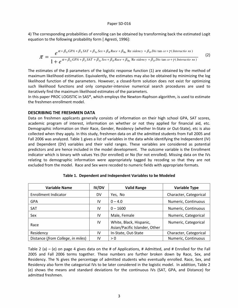
4) The corresponding probabilities of enrolling can be obtained by transforming back the estimated Logit

equation to the following probability form [ Agresti, 1996]:

(2)

The estimates of the β parameters of the logistic response function (1) are obtained by the method of

maximum likelihood estimation. Equivalently, the estimates may also be obtained by minimizing the log

likelihood function of the parameters. However, a closed-form solution does not exist for optimizing

such likelihood functions and only computer-intensive numerical search procedures are used to

iteratively find the maximum likelihood estimates of the parameters.

In this paper PROC LOGISTIC in SAS®, which employs the Newton-Raphson algorithm, is used to estimate

the freshmen enrollment model.

DESCRIBING THE FRESHMEN DATA Data on freshmen applicants generally consists of information on their high school GPA, SAT scores,

academic program of interest, information on whether or not they applied for financial aid, etc.

Demographic information on their Race, Gender, Residency (whether In-State or Out-State), etc is also

collected when they apply. In this study, freshmen data on all the admitted students from Fall 2005 and

Fall 2006 was analyzed. Table 1 gives a list of variables in the data while identifying the Independent (IV)

and Dependent (DV) variables and their valid ranges. These variables are considered as potential

predictors and are hence included in the model development. The outcome variable is the Enrollment

indicator which is binary with values Yes (for enrolled) or No (for not enrolled). Missing data on the IVs

relating to demographic information were appropriately tagged by recoding so that they are not

excluded from the model. Race and Sex were recoded to numeric fields with appropriate formats.

Table 1. Dependent and Independent Variables to be Modeled

Variable Name IV/DV Valid Range Variable Type

Enrollment Indicator DV Yes, No Character, Categorical

GPA IV 0 – 4.0 Numeric, Continuous

SAT IV 0 – 1600 Numeric, Continuous

Sex IV Male, Female Numeric, Categorical

Race IV White, Black, Hispanic,

Asian/Pacific Islander, Other

Numeric, Categorical

Residency IV In-State, Out-State Character, Categorical

Distance (from College, in miles) IV > 0 Numeric, Continuous

Table 2 (a) – (e) on page 4 gives data on the # of Applications, # Admitted, and # Enrolled for the Fall

2005 and Fall 2006 terms together. These numbers are further broken down by Race, Sex, and

Residency. The % gives the percentage of admitted students who eventually enrolled. Race, Sex, and

Residency also form the categorical IVs to be later considered in the logistic model. In addition, Table 2

(e) shows the means and standard deviations for the continuous IVs (SAT, GPA, and Distance) for

admitted freshmen.

)(tanRe

)(tanRe

Re

Re

1nsInteractioceDissidencyRaceSexSATGPA

nsInteractioceDissidencyRaceSexSATGPA

DRSeSG

DRSeSG

e

eγββββββα

γββββββα

π+++++++

+++++++

+=

Paper SD-016

4

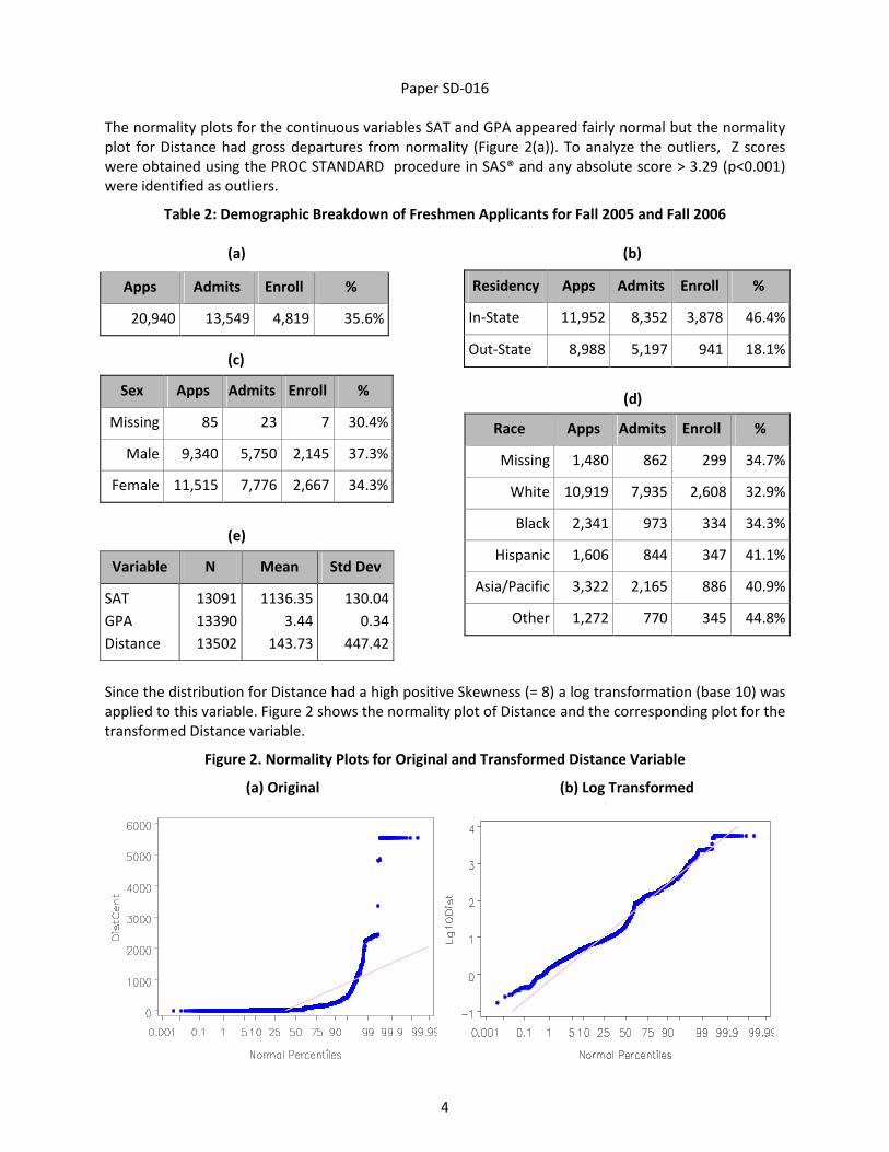
The normality plots for the continuous variables SAT and GPA appeared fairly normal but the normality

plot for Distance had gross departures from normality (Figure 2(a)). To analyze the outliers, Z scores

were obtained using the PROC STANDARD procedure in SAS® and any absolute score > 3.29 (p<0.001)

were identified as outliers.

Table 2: Demographic Breakdown of Freshmen Applicants for Fall 2005 and Fall 2006

(a) (b)

(c)

(d)

(e)

Since the distribution for Distance had a high positive Skewness (= 8) a log transformation (base 10) was

applied to this variable. Figure 2 shows the normality plot of Distance and the corresponding plot for the

transformed Distance variable.

Figure 2. Normality Plots for Original and Transformed Distance Variable

(a) Original (b) Log Transformed

Apps Admits Enroll %

20,940 13,549 4,819 35.6%

Residency Apps Admits Enroll %

In-State 11,952 8,352 3,878 46.4%

Out-State 8,988 5,197 941 18.1%

Sex Apps Admits Enroll %

Missing 85 23 7 30.4%

Male 9,340 5,750 2,145 37.3%

Female 11,515 7,776 2,667 34.3%

Race Apps Admits Enroll %

Missing 1,480 862 299 34.7%

White 10,919 7,935 2,608 32.9%

Black 2,341 973 334 34.3%

Hispanic 1,606 844 347 41.1%

Asia/Pacific 3,322 2,165 886 40.9%

Other 1,272 770 345 44.8%

Variable N Mean Std Dev

SAT

GPA

Distance

13091

13390

13502

1136.35

3.44

143.73

130.04

0.34

447.42

Paper SD-016

5

DATA EXPLORATION VIA VISUALIZATION Preliminary data exploration of the IV-DV relationship gives useful information on the associations which

can be later incorporated into the Logit model. Figure 3 shows the box plots for GPA for those admitted

freshmen who did and didn’t enroll, broken down by Sex. Similar plots were obtained for the IV SAT and

they displayed the same pattern.

Figure 3. Box Plots of GPA

The bars are represented by MY (Males

who enrolled), MN (Males who didn’t

enroll), FY (Females who enrolled), and

FN (Females who didn’t enroll). The

average GPA for those who enrolled is

less than the average GPA for the ones

who did not enroll. This pattern is

consistent amongst Males and Females

and the same pattern was obtained

across the IVs Race and Residency. Since

many plots had to be generated

repetitively the following macro (SAS®

Code 1), using PROC BOXPLOTS in SAS®,

was developed to control the axis

variables and all other graphical aspects.

Boxplots: Response=Enroll, Predictor=GPA, Control=Sex

Sex: M F

MY MN FY FN

2.00

2.25

2.50

2.75

3.00

3.25

3.50

3.75

4.00

GPA

Enrollment Indicator

Mean=3.44

SAS® CODE 1

%MACRO OUTLIER(T1=, N=, W=, B1=, LL=, T2=, V1=, G1=, VA1=, VR1=, VL1=, TL=);

PROC SORT DATA=NENROL.FALLACCEP0506 OUT=BOX;

BY &B1. DESCENDING ENROL_IND;

RUN;

/** SETTING PLOT DISPLAY ATTRIBUTES*/

SYMBOL1 V=CIRCLE C=RED; SYMBOL2 V=SQUARE C=RED;

AXIS1 LABEL=(FONT=VERDANA HEIGHT=1.8 "ENROLLMENT INDICATOR")

VALUE=(FONT=VERDANA HEIGHT = 1.8 &TL.);

LEGEND1 LABEL= (FONT=VERDANA HEIGHT=1.6 "&B1.:") ACROSS=&N. POSITION=(TOP CENTER

OUTSIDE) CBORDER=BLACK CFRAME=CXFFFF88

VALUE= (JUSTIFY=LEFT FONT=VERDANA HEIGHT=1.6 &LL.);

TITLE COLOR=BLACK FONT=VERDANA HEIGHT=2.0 "BOXPLOTS: RESPONSE=ENROLL,

PREDICTOR=&T1.&T2.";

PROC BOXPLOT DATA=BOX;

PLOT &V1.*ENROL_IND&G1./ BOXSTYLE=SCHEMATICID HEIGHT=4.2 VOFFSET=3

HOFFSET=2 CBOXFILL=(BXCL) FONT=VERDANA

IDSYMBOL=CIRCLE VAXIS=&VA1.

VREF=&VR1. VREFLABELS=&VL1. VREFLABPOS=3

CVREF=GREEN LVREF=20 SYMBOLLEGEND=LEGEND1

SYMBOLORDER=DATA HAXIS=AXIS1;

&W. ;

RUN;

%MEND OUTLIER;

/* CALLING MACRO OUTLIER TO PLOT THE BOXPLOT FOR GPA IN FIGURE 3 */

%OUTLIER(T1=GPA, N=2, W= WHERE SEX NE 0 %STR(;), B1=SEX, LL= 'M' 'F', T2=%STR(,)

CONTROL%STR(=)&B1., V1=GPA, G1= %STR(=)&B1., VA1=2.0 2.25 2.5 2.75 3.0

3.25 3.5 3.75 4.0, VR1=3.44, VL1="MEAN=3.44", TL='MY' 'MN' 'FY' 'FN')

Paper SD-016

6

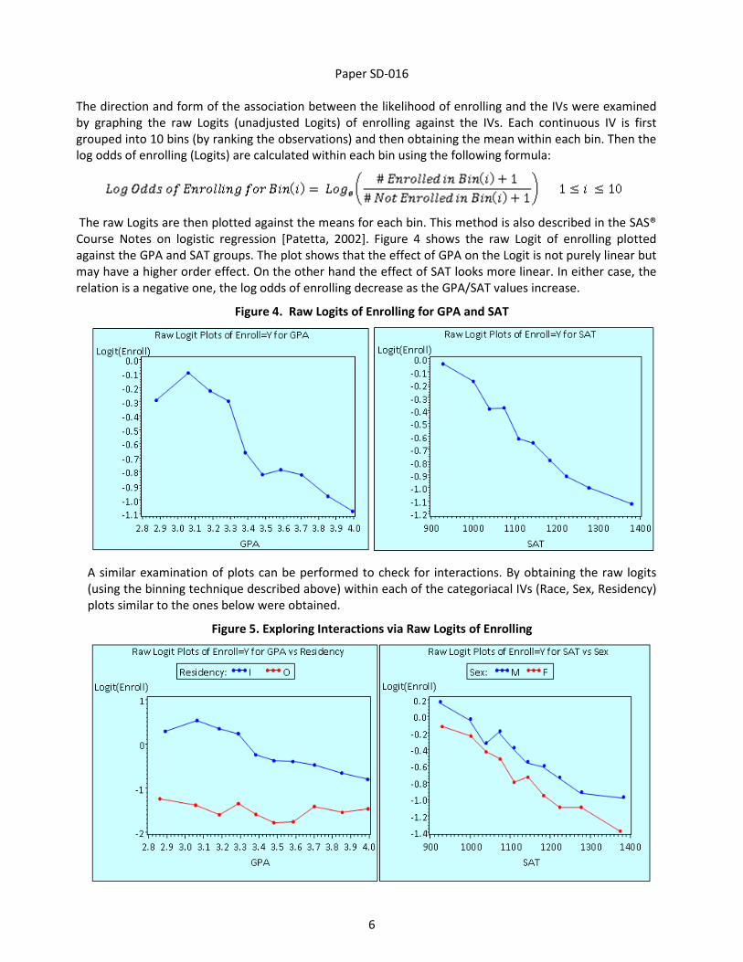
The direction and form of the association between the likelihood of enrolling and the IVs were examined

by graphing the raw Logits (unadjusted Logits) of enrolling against the IVs. Each continuous IV is first

grouped into 10 bins (by ranking the observations) and then obtaining the mean within each bin. Then the

log odds of enrolling (Logits) are calculated within each bin using the following formula:

The raw Logits are then plotted against the means for each bin. This method is also described in the SAS®

Course Notes on logistic regression [Patetta, 2002]. Figure 4 shows the raw Logit of enrolling plotted

against the GPA and SAT groups. The plot shows that the effect of GPA on the Logit is not purely linear but

may have a higher order effect. On the other hand the effect of SAT looks more linear. In either case, the

relation is a negative one, the log odds of enrolling decrease as the GPA/SAT values increase.

Figure 4. Raw Logits of Enrolling for GPA and SAT

A similar examination of plots can be performed to check for interactions. By obtaining the raw logits

(using the binning technique described above) within each of the categoriacal IVs (Race, Sex, Residency)

plots similar to the ones below were obtained.

Figure 5. Exploring Interactions via Raw Logits of Enrolling

Paper SD-016

7

Figure 5 (page 6) shows that there may be a GPA*Residency interaction effect present since the lines for

I (In-State) and O (Out-State) seem to be converging at some point. On the other hand the lines for M

(Males) and F (Females) look parallel with respect to SAT indicating there may not be a SAT*Sex

interaction present. These preliminary plots only give approximate indications of the form of the IVs that

may be expected to be seen as significant in the final estimated logistic model. They are approximate

because the associations have not been controlled (adjusted) for the presence of the other IVs.

LOGISTIC REGRESSION MODEL FOR GMU FRESHMEN DATA This section discusses the fitting of the multiple logistic regression model to predict the probability of

the binary response, Enrollment (Yes, No), of admitted GMU freshmen using the predictors GPA, SAT,

Distance (log transformed), Residency, Race, and Sex. About 5% of the observations had missing values

for GPA, SAT, or Distance and were deleted case wise from the analysis automatically. The reference

category for class variables is White, Female, Out-State which correspond to the three class variables

Race, Sex, and Residency respectively.

SAS® Code 2 shows the PROC LOGISTIC code that was employed using reference parameterization

(PARAM=REF) and backward selection (SELECTION=BACKWARD) with 5% significance criterion

(SLSTAY=0.05) for the effects to be retained in the model. The TECH=NEWTON specifies the use of the

Newton-Raphson optimization method of estimation instead of the default Fisher Scoring. Models up to

the 2nd

order interaction were considered since it becomes more and more complex to give practical

interpretations of higher order interactions.

Maximum Likelihood Estimation: The likelihood function (L) expresses the probability of the observed

data as a function of the unknown parameters. The parameters are then estimated by maximizing this

function or equivalently minimizing -2Log L. A Logit model is obtained by first starting with the most

complex form that one is willing to consider and evaluating the -2Log L. The change in the -2Log L is

noted in terms of the P-value by dropping the highest order terms one by one and comparing the new

value with the previous one. The term that leads to the least significant change in the -2Log L is now

completely dropped from the model and the new -2Log L is now used for comparison. This process

continues till there are no more terms whose omission lead to a non-significant change in the -2Log L.

The terms are dropped by maintaining hierarchy, that is, terms involved in significant higher order

interactions are not dropped even though they may be non-significant by themselves.

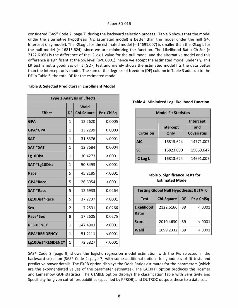
Fit Statistics: Table 3 (page 8) shows the main effects and the interactions effects retained in the final

model along with the Chi-Sqr values. All the effects show significance at the 5% level. As was noted from

the raw logit plots there is a strong GPA*Residency interaction effect (p<0.0001), which means that the

change in log odds of enrolling due to a unit change in GPA is different for In-State and Out-State

freshmen students. Two other important interactions are GPA*Race and SAT*Race, both of which are

highly significant. Table 4 shows the final value of the minimized -2Log L function (=14691.007)

generating the parameter estimates. This is the smallest value amongst the class of models that were

SAS® CODE 2

PROC LOGISTIC DATA=NENROL.FALLACCEP0506 DESCENDING; /* MODELS ENROL_IND=Y */

CLASS RACE (REF='1-WHITE') RESIDENCY (REF=LAST) SEX (REF=LAST)

/PARAM=REF ORDER=INTERNAL; /* REF: WHITE, FEMALES, OUT-STATE*/

MODEL ENROL_IND = GPA|GPA*GPA|SAT_HIGHTOT|SAT_HIGHTOT*SAT_HIGHTOT|LG10DIST|

RACE|SEX|RESIDENCY @2/

TECH = NEWTON

SELECTION=BACKWARD HIERARCHY=SINGLE SLSTAY=.05;

RUN;

Paper SD-016

8

considered (SAS® Code 2, page 7) during the backward selection process. Table 5 shows that the model

under the alternative hypothesis (HA: Estimated model) is better than the model under the null (H0:

Intercept only model). The -2Log L for the estimated model (= 14691.007) is smaller than the -2Log L for

the null model (= 16813.624), since we are minimizing the function. The Likelihood Ratio Ch-Sqr (=

2122.6166) is the difference of the -2Log L value for the null model and the alternative model and this

difference is significant at the 5% level (p<0.0001), hence we accept the estimated model under HA. This

LR test is not a goodness of fit (GOF) test and merely shows the estimated model fits the data better

than the Intercept only model. The sum of the degrees of freedom (DF) column in Table 3 adds up to the

DF in Table 5, the total DF for the estimated model.

Table 3. Selected Predictors in Enrollment Model

Table 4. Minimized Log Likelihood Function

Table 5. Significance Tests for

Estimated Model

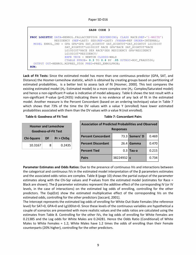
SAS® Code 3 (page 9) shows the logistic regression model estimation with the IVs selected in the

backward selection (SAS® Code 2, page 7) with some additional options for goodness of fit tests and

predictive power details. The EXPB option displays the Odds Ratios estimates for the parameters (which

are the exponentiated values of the parameter estimates). The LACKFIT option produces the Hosmer

and Lemeshow GOF statistics. The CTABLE option displays the classification table with Sensitivity and

Specificity for given cut-off probabilities (specified by PPROB) and OUTROC outputs these to a data set.

Type 3 Analysis of Effects

Effect DF

Wald

Chi-Square Pr > ChiSq

GPA 1 12.2620 0.0005

GPA*GPA 1 13.2299 0.0003

SAT 1 31.8376 <.0001

SAT *SAT 1 12.7684 0.0004

Lg10Dist 1 30.4273 <.0001

SAT *Lg10Dist 1 50.8493 <.0001

Race 5 45.2185 <.0001

GPA*Race 5 26.6954 <.0001

SAT *Race 5 12.6933 0.0264

Lg10Dist*Race 5 37.2737 <.0001

Sex 2 7.2531 0.0266

Race*Sex 8 17.2605 0.0275

RESIDENCY 1 147.4903 <.0001

GPA*RESIDENCY 1 51.2111 <.0001

Lg10Dist*RESIDENCY 1 72.5827 <.0001

Model Fit Statistics

Criterion

Intercept

Only

Intercept

and

Covariates

AIC 16815.624 14771.007

SC 16823.090 15069.647

-2 Log L 16813.624 14691.007

Testing Global Null Hypothesis: BETA=0

Test Chi-Square DF Pr > ChiSq

Likelihood

Ratio

2122.6166 39 <.0001

Score 2010.4630 39 <.0001

Wald 1699.2332 39 <.0001

Paper SD-016

9

Lack of Fit Tests: Since the estimated model has more than one continuous predictor (GPA, SAT, and

Distance) the Hosmer-Lemeshow statistic, which is obtained by creating groups based on partitioning of

estimated probabilities, is a better test to assess lack of fit [Hosmer, 2000]. This test compares the

existing estimated model (H0: Estimated model) to a more complex one (HA: Complex/Saturated model)

and hence a non-significant P-value is indicative of model adequacy. Table 6 shows the test result with a

non-significant P-value (p=0.2435) indicating there is no evidence of any lack of fit in the estimated

model. Another measure is the Percent Concordant (based on an ordering technique) value in Table 7

which shows that 73% of the time the DV values with a value Y (enrolled) have lower estimated

probabilities associated with them than the DV values with a value N (not enrolled).

Table 6: Goodness of Fit Test Table 7: Concordant Pairs

Hosmer and Lemeshow

Goodness-of-Fit Test

Chi-Square DF Pr > ChiSq

10.3167 8 0.2435

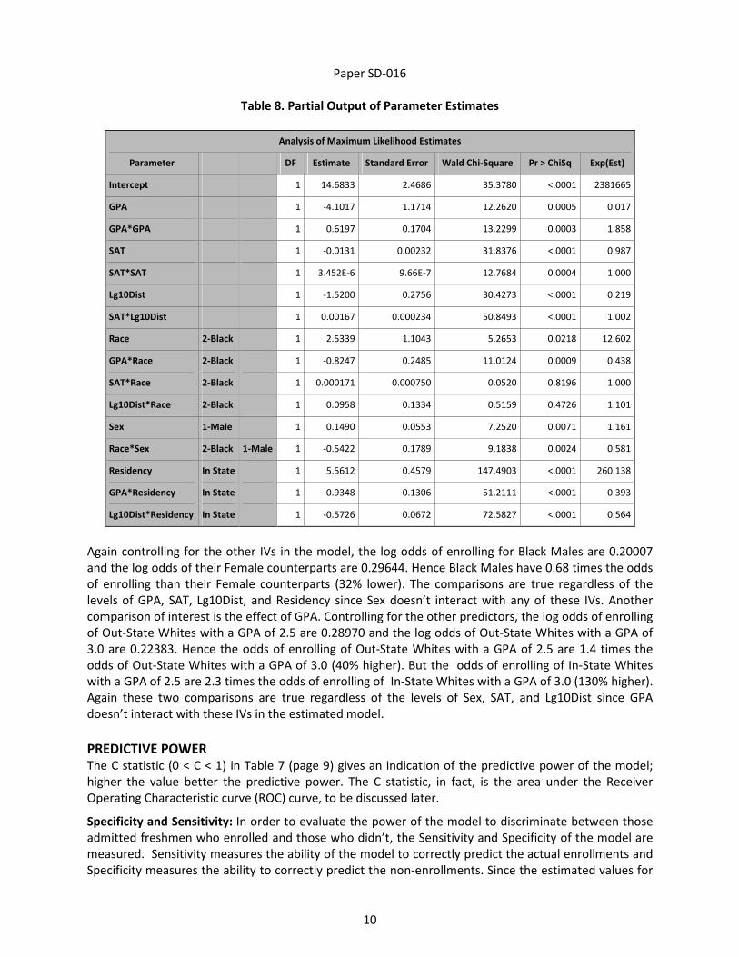
Parameter Estimates and Odds Ratios: Due to the presence of continuous IVs and interactions between

the categorical and continuous IVs in the estimated model interpretation of the β parameters estimates

and the associated odds ratios are complex. Table 8 (page 10) shows the partial output of the parameter

estimates along with the Chi-Sqr values and P-values from the estimated model (estimates for Race =

Black are shown). The β parameter estimates represent the additive effect of the corresponding IV (or IV

levels, in the case of interactions) on the estimated log odds of enrolling, controlling for the other

predictors. The Exp(Est) show the estimated multiplicative effect of the corresponding IVs on the

estimated odds, controlling for the other predictors [Jaccard, 2001].

The Intercept represents the estimated log odds of enrolling for White Out-State Females (the reference

level) for SAT=0, GPA=0 and Lg10Dist=0. Since these levels of the continuous variables are hypothetical a

couple of scenarios are presented with more realistic values and the odds ratios are calculated using the

estimates from Table 8. Controlling for the other IVs, the log odds of enrolling for White Females are

0.21385 and the Log odds for White Males are 0.24281. Hence the Odds Ratio (Conditional) of White

Males to White Females ≈ 1.2; White Males have 1.2 times the odds of enrolling than their Female

counterparts (20% higher), controlling for the other predictors.

Association of Predicted Probabilities and Observed

Responses

Percent Concordant 73.3 Somers' D 0.469

Percent Discordant 26.4 Gamma 0.470

Percent Tied 0.3 Tau-a 0.215

Pairs 38224932 c 0.734

SAS® CODE 3

PROC LOGISTIC DATA=NENROL.FALLACCEP0506 DESCENDING; CLASS RACE(REF='1-WHITE')

RESIDENCY (REF=LAST) SEX(REF=LAST) /PARAM=REF ORDER=INTERNAL;

MODEL ENROL_IND = GPA GPA*GPA SAT_HIGHTOT SAT_HIGHTOT*SAT_HIGHTOT LG10DIST

SAT_HIGHTOT*LG10DIST RACE GPA*RACE SAT_HIGHTOT*RACE

LG10DIST*RACE SEX RACE*SEX RESIDENCY GPA*RESIDENCY

LG10DIST*RESIDENCY/

EXPB TECH = NEWTON CLODDS=WALD

CTABLE PPROB= 0.3 TO 0.6 BY .05 OUTROC=ROC_FRAD0506;

OUTPUT OUT=NENROL.M2PRED_0506 PRED=PRED_ENROLPROB;

RUN;

Paper SD-016

10

Table 8. Partial Output of Parameter Estimates

Analysis of Maximum Likelihood Estimates

Parameter DF Estimate Standard Error Wald Chi-Square Pr > ChiSq Exp(Est)

Intercept 1 14.6833 2.4686 35.3780 <.0001 2381665

GPA 1 -4.1017 1.1714 12.2620 0.0005 0.017

GPA*GPA 1 0.6197 0.1704 13.2299 0.0003 1.858

SAT 1 -0.0131 0.00232 31.8376 <.0001 0.987

SAT*SAT 1 3.452E-6 9.66E-7 12.7684 0.0004 1.000

Lg10Dist 1 -1.5200 0.2756 30.4273 <.0001 0.219

SAT*Lg10Dist 1 0.00167 0.000234 50.8493 <.0001 1.002

Race 2-Black 1 2.5339 1.1043 5.2653 0.0218 12.602

GPA*Race 2-Black 1 -0.8247 0.2485 11.0124 0.0009 0.438

SAT*Race 2-Black 1 0.000171 0.000750 0.0520 0.8196 1.000

Lg10Dist*Race 2-Black 1 0.0958 0.1334 0.5159 0.4726 1.101

Sex 1-Male 1 0.1490 0.0553 7.2520 0.0071 1.161

Race*Sex 2-Black 1-Male 1 -0.5422 0.1789 9.1838 0.0024 0.581

Residency In State 1 5.5612 0.4579 147.4903 <.0001 260.138

GPA*Residency In State 1 -0.9348 0.1306 51.2111 <.0001 0.393

Lg10Dist*Residency In State 1 -0.5726 0.0672 72.5827 <.0001 0.564

Again controlling for the other IVs in the model, the log odds of enrolling for Black Males are 0.20007

and the log odds of their Female counterparts are 0.29644. Hence Black Males have 0.68 times the odds

of enrolling than their Female counterparts (32% lower). The comparisons are true regardless of the

levels of GPA, SAT, Lg10Dist, and Residency since Sex doesn’t interact with any of these IVs. Another

comparison of interest is the effect of GPA. Controlling for the other predictors, the log odds of enrolling

of Out-State Whites with a GPA of 2.5 are 0.28970 and the log odds of Out-State Whites with a GPA of

3.0 are 0.22383. Hence the odds of enrolling of Out-State Whites with a GPA of 2.5 are 1.4 times the

odds of Out-State Whites with a GPA of 3.0 (40% higher). But the odds of enrolling of In-State Whites

with a GPA of 2.5 are 2.3 times the odds of enrolling of In-State Whites with a GPA of 3.0 (130% higher).

Again these two comparisons are true regardless of the levels of Sex, SAT, and Lg10Dist since GPA

doesn’t interact with these IVs in the estimated model.

PREDICTIVE POWER The C statistic (0 < C < 1) in Table 7 (page 9) gives an indication of the predictive power of the model;

higher the value better the predictive power. The C statistic, in fact, is the area under the Receiver

Operating Characteristic curve (ROC) curve, to be discussed later.

Specificity and Sensitivity: In order to evaluate the power of the model to discriminate between those

admitted freshmen who enrolled and those who didn’t, the Sensitivity and Specificity of the model are

measured. Sensitivity measures the ability of the model to correctly predict the actual enrollments and

Specificity measures the ability to correctly predict the non-enrollments. Since the estimated values for

Paper SD-016

11

the DV (enrollment status) are probabilities lying between 0 and 1, the classification of the estimated

probabilities (into enrolled and not enrolled) depends on a particular cut-off probability value. This cut-

off is selected depending on the field of research and the protocols involved in the field. In an ideal case,

both Sensitivity and Specificity should be high for this cut-off. For the Office of Admissions a student

estimated to have a 35% to 40% chance of enrolling is a positive indication of yield. Hence a probability

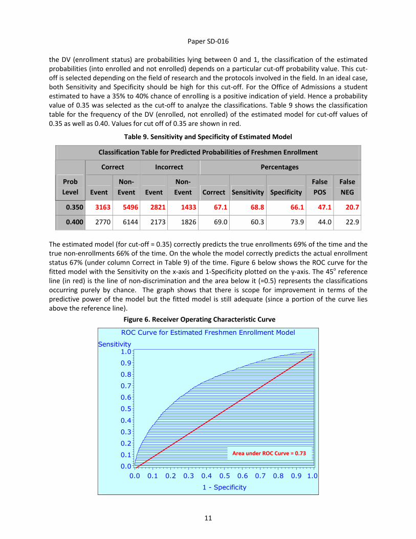
value of 0.35 was selected as the cut-off to analyze the classifications. Table 9 shows the classification

table for the frequency of the DV (enrolled, not enrolled) of the estimated model for cut-off values of

0.35 as well as 0.40. Values for cut off of 0.35 are shown in red.

Table 9. Sensitivity and Specificity of Estimated Model

Classification Table for Predicted Probabilities of Freshmen Enrollment

Correct Incorrect Percentages

Prob

Level Event

Non-

Event Event

Non-

Event Correct Sensitivity Specificity

False

POS

False

NEG

0.350 3163 5496 2821 1433 67.1 68.8 66.1 47.1 20.7

0.400 2770 6144 2173 1826 69.0 60.3 73.9 44.0 22.9

The estimated model (for cut-off = 0.35) correctly predicts the true enrollments 69% of the time and the

true non-enrollments 66% of the time. On the whole the model correctly predicts the actual enrollment

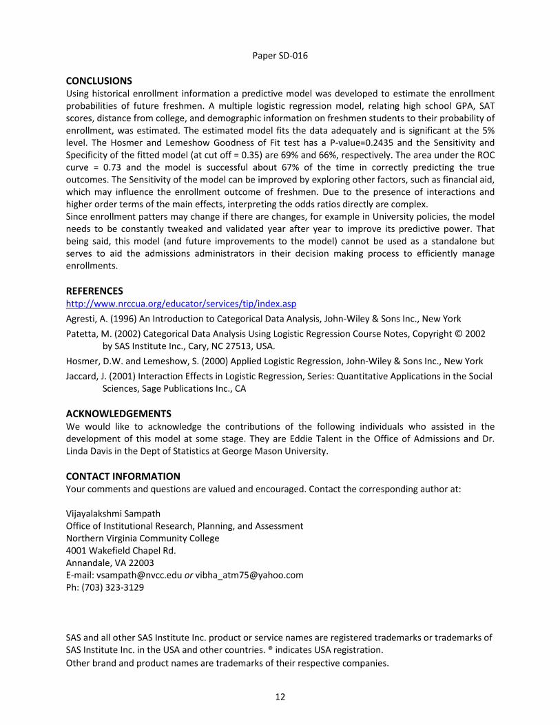
status 67% (under column Correct in Table 9) of the time. Figure 6 below shows the ROC curve for the

fitted model with the Sensitivity on the x-axis and 1-Specificity plotted on the y-axis. The 45o reference

line (in red) is the line of non-discrimination and the area below it (=0.5) represents the classifications

occurring purely by chance. The graph shows that there is scope for improvement in terms of the

predictive power of the model but the fitted model is still adequate (since a portion of the curve lies

above the reference line).

Figure 6. Receiver Operating Characteristic Curve

ROC Curve for Estimated Freshmen Enrollment Model

Sensitivity

0.0

0.1

0.2

0.3

0.4

0.5

0.6

0.7

0.8

0.9

1.0

1 - Specificity

0.0 0.1 0.2 0.3 0.4 0.5 0.6 0.7 0.8 0.9 1.0

Area under ROC Curve = 0.73

Paper SD-016

12

CONCLUSIONS Using historical enrollment information a predictive model was developed to estimate the enrollment

probabilities of future freshmen. A multiple logistic regression model, relating high school GPA, SAT

scores, distance from college, and demographic information on freshmen students to their probability of

enrollment, was estimated. The estimated model fits the data adequately and is significant at the 5%

level. The Hosmer and Lemeshow Goodness of Fit test has a P-value=0.2435 and the Sensitivity and

Specificity of the fitted model (at cut off = 0.35) are 69% and 66%, respectively. The area under the ROC

curve = 0.73 and the model is successful about 67% of the time in correctly predicting the true

outcomes. The Sensitivity of the model can be improved by exploring other factors, such as financial aid,

which may influence the enrollment outcome of freshmen. Due to the presence of interactions and

higher order terms of the main effects, interpreting the odds ratios directly are complex.

Since enrollment patters may change if there are changes, for example in University policies, the model

needs to be constantly tweaked and validated year after year to improve its predictive power. That

being said, this model (and future improvements to the model) cannot be used as a standalone but

serves to aid the admissions administrators in their decision making process to efficiently manage

enrollments.

REFERENCES http://www.nrccua.org/educator/services/tip/index.asp

Agresti, A. (1996) An Introduction to Categorical Data Analysis, John-Wiley & Sons Inc., New York

Patetta, M. (2002) Categorical Data Analysis Using Logistic Regression Course Notes, Copyright © 2002

by SAS Institute Inc., Cary, NC 27513, USA.

Hosmer, D.W. and Lemeshow, S. (2000) Applied Logistic Regression, John-Wiley & Sons Inc., New York

Jaccard, J. (2001) Interaction Effects in Logistic Regression, Series: Quantitative Applications in the Social

Sciences, Sage Publications Inc., CA

ACKNOWLEDGEMENTS

We would like to acknowledge the contributions of the following individuals who assisted in the

development of this model at some stage. They are Eddie Talent in the Office of Admissions and Dr.

Linda Davis in the Dept of Statistics at George Mason University.

CONTACT INFORMATION Your comments and questions are valued and encouraged. Contact the corresponding author at:

Vijayalakshmi Sampath

Office of Institutional Research, Planning, and Assessment

Northern Virginia Community College

4001 Wakefield Chapel Rd.

Annandale, VA 22003

E-mail: vsampath@nvcc.edu or vibha_atm75@yahoo.com

Ph: (703) 323-3129

SAS and all other SAS Institute Inc. product or service names are registered trademarks or trademarks of

SAS Institute Inc. in the USA and other countries. ® indicates USA registration.

Other brand and product names are trademarks of their respective companies.