a little book of r for biomedical statistics - read the docs · a little book of r for biomedical...

A Little Book of R For BiomedicalStatistics

Release 0.2

Avril Coghlan

December 17, 2016

Contents

1 How to install R 31.1 Introduction to R . . . . . . . . . . . . . . . . . . . . . . . . . . . . . . . . . . . . . . . . . . . 31.2 Installing R . . . . . . . . . . . . . . . . . . . . . . . . . . . . . . . . . . . . . . . . . . . . . . 3

1.2.1 How to check if R is installed on a Windows PC . . . . . . . . . . . . . . . . . . . . . . 31.2.2 Finding out what is the latest version of R . . . . . . . . . . . . . . . . . . . . . . . . . 31.2.3 Installing R on a Windows PC . . . . . . . . . . . . . . . . . . . . . . . . . . . . . . . 41.2.4 How to install R on non-Windows computers (eg. Macintosh or Linux computers) . . . . 5

1.3 Installing R packages . . . . . . . . . . . . . . . . . . . . . . . . . . . . . . . . . . . . . . . . . 51.3.1 How to install an R package . . . . . . . . . . . . . . . . . . . . . . . . . . . . . . . . 51.3.2 How to install a Bioconductor R package . . . . . . . . . . . . . . . . . . . . . . . . . 6

1.4 Running R . . . . . . . . . . . . . . . . . . . . . . . . . . . . . . . . . . . . . . . . . . . . . . 71.5 A brief introduction to R . . . . . . . . . . . . . . . . . . . . . . . . . . . . . . . . . . . . . . . 71.6 Links and Further Reading . . . . . . . . . . . . . . . . . . . . . . . . . . . . . . . . . . . . . . 101.7 Acknowledgements . . . . . . . . . . . . . . . . . . . . . . . . . . . . . . . . . . . . . . . . . 101.8 Contact . . . . . . . . . . . . . . . . . . . . . . . . . . . . . . . . . . . . . . . . . . . . . . . . 101.9 License . . . . . . . . . . . . . . . . . . . . . . . . . . . . . . . . . . . . . . . . . . . . . . . . 10

2 Using R for Biomedical Statistics 112.1 Biomedical statistics . . . . . . . . . . . . . . . . . . . . . . . . . . . . . . . . . . . . . . . . . 112.2 Calculating Relative Risks for a Cohort Study . . . . . . . . . . . . . . . . . . . . . . . . . . . . 112.3 Calculating Odds Ratios for a Cohort or Case-Control Study . . . . . . . . . . . . . . . . . . . . 132.4 Testing for an Association Between Disease and Exposure, in a Cohort or Case-Control Study . . 152.5 Calculating the (Mantel-Haenszel) Odds Ratio when there is a Stratifying Variable . . . . . . . . 152.6 Testing for an Association Between Exposure and Disease in a Matched Case-Control Study . . . 182.7 Dose-response analysis: . . . . . . . . . . . . . . . . . . . . . . . . . . . . . . . . . . . . . . . 192.8 Calculating the Sample Size Required for a Randomised Control Trial . . . . . . . . . . . . . . . 212.9 Calculating the Power of a Randomised Control Trial . . . . . . . . . . . . . . . . . . . . . . . . 222.10 Making a Forest Plot for a Meta-analysis of Several Different Randomised Control Trials: . . . . 232.11 Links and Further Reading . . . . . . . . . . . . . . . . . . . . . . . . . . . . . . . . . . . . . . 252.12 Acknowledgements . . . . . . . . . . . . . . . . . . . . . . . . . . . . . . . . . . . . . . . . . 252.13 Contact . . . . . . . . . . . . . . . . . . . . . . . . . . . . . . . . . . . . . . . . . . . . . . . . 262.14 License . . . . . . . . . . . . . . . . . . . . . . . . . . . . . . . . . . . . . . . . . . . . . . . . 26

3 Acknowledgements 27

4 Contact 29

5 License 31

i

A Little Book of R For Biomedical Statistics, Release 0.2

By Avril Coghlan, Parasite Genomics Group, Wellcome Trust Sanger Institute, Cambridge, U.K. Email:[email protected]

This is a simple introduction to biomedical statistics using the R statistics software.

There is a pdf version of this booklet available at https://media.readthedocs.org/pdf/a-little-book-of-r-for-biomedical-statistics/latest/a-little-book-of-r-for-biomedical-statistics.pdf.

If you like this booklet, you may also like to check out my booklet on using R for time series analysis, http://a-little-book-of-r-for-time-series.readthedocs.org/ and my booklet on using R for multivariate analysis, http://little-book-of-r-for-multivariate-analysis.readthedocs.org/.

Contents:

Contents 1

http://www.sanger.ac.uk/research/projects/parasitegenomics/

mailto:[email protected]

https://media.readthedocs.org/pdf/a-little-book-of-r-for-biomedical-statistics/latest/a-little-book-of-r-for-biomedical-statistics.pdf


http://a-little-book-of-r-for-time-series.readthedocs.org/


http://little-book-of-r-for-multivariate-analysis.readthedocs.org/



2 Contents

CHAPTER 1

How to install R

1.1 Introduction to R

This little booklet has some information on how to use R for biomedical statistics.

R (www.r-project.org) is a commonly used free Statistics software. R allows you to carry out statistical analysesin an interactive mode, as well as allowing simple programming.

1.2 Installing R

To use R, you first need to install the R program on your computer.

1.2.1 How to check if R is installed on a Windows PC

Before you install R on your computer, the first thing to do is to check whether R is already installed on yourcomputer (for example, by a previous user).

These instructions will focus on installing R on a Windows PC. However, I will also briefly mention how to installR on a Macintosh or Linux computer (see below).

If you are using a Windows PC, there are two ways you can check whether R is already isntalled on your computer:

1. Check if there is an “R” icon on the desktop of the computer that you are using. If so, double-click on the“R” icon to start R. If you cannot find an “R” icon, try step 2 instead.

2. Click on the “Start” menu at the bottom left of your Windows desktop, and then move your mouse over“All Programs” in the menu that pops up. See if “R” appears in the list of programs that pops up. If it does,it means that R is already installed on your computer, and you can start R by selecting “R” (or R X.X.X,where X.X.X gives the version of R, eg. R 2.10.0) from the list.

If either (1) or (2) above does succeed in starting R, it means that R is already installed on the computer that youare using. (If neither succeeds, R is not installed yet). If there is an old version of R installed on the Windows PCthat you are using, it is worth installing the latest version of R, to make sure that you have all the latest R functionsavailable to you to use.

1.2.2 Finding out what is the latest version of R

To find out what is the latest version of R, you can look at the CRAN (Comprehensive R Network) website,http://cran.r-project.org/.

Beside “The latest release” (about half way down the page), it will say something like “R-X.X.X.tar.gz” (eg.“R-2.12.1.tar.gz”). This means that the latest release of R is X.X.X (for example, 2.12.1).

3

http://www.r-project.org/

http://cran.r-project.org/


New releases of R are made very regularly (approximately once a month), as R is actively being improved all thetime. It is worthwhile installing new versions of R regularly, to make sure that you have a recent version of R (toensure compatibility with all the latest versions of the R packages that you have downloaded).

1.2.3 Installing R on a Windows PC

To install R on your Windows computer, follow these steps:

1. Go to http://ftp.heanet.ie/mirrors/cran.r-project.org.

2. Under “Download and Install R”, click on the “Windows” link.

3. Under “Subdirectories”, click on the “base” link.

4. On the next page, you should see a link saying something like “Download R 2.10.1 for Windows” (or RX.X.X, where X.X.X gives the version of R, eg. R 2.11.1). Click on this link.

5. You may be asked if you want to save or run a file “R-2.10.1-win32.exe”. Choose “Save” and save the fileon the Desktop. Then double-click on the icon for the file to run it.

6. You will be asked what language to install it in - choose English.

7. The R Setup Wizard will appear in a window. Click “Next” at the bottom of the R Setup wizard window.

8. The next page says “Information” at the top. Click “Next” again.

9. The next page says “Information” at the top. Click “Next” again.

10. The next page says “Select Destination Location” at the top. By default, it will suggest to install R in“C:\Program Files” on your computer.

11. Click “Next” at the bottom of the R Setup wizard window.

12. The next page says “Select components” at the top. Click “Next” again.

13. The next page says “Startup options” at the top. Click “Next” again.

14. The next page says “Select start menu folder” at the top. Click “Next” again.

15. The next page says “Select additional tasks” at the top. Click “Next” again.

16. R should now be installed. This will take about a minute. When R has finished, you will see “Completingthe R for Windows Setup Wizard” appear. Click “Finish”.

17. To start R, you can either follow step 18, or 19:


19. Click on the “Start” button at the bottom left of your computer screen, and then choose “All programs”, andstart R by selecting “R” (or R X.X.X, where X.X.X gives the version of R, eg. R 2.10.0) from the menu ofprograms.

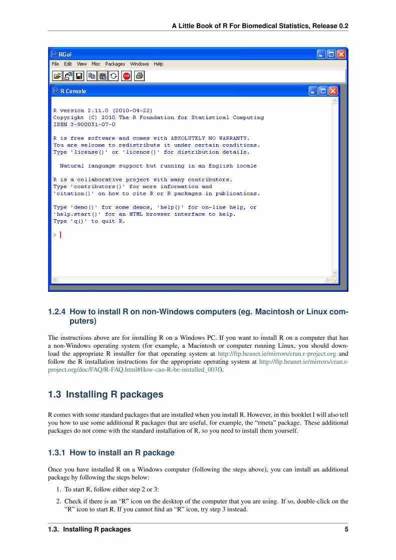
20. The R console (a rectangle) should pop up:

4 Chapter 1. How to install R

http://ftp.heanet.ie/mirrors/cran.r-project.org


1.2.4 How to install R on non-Windows computers (eg. Macintosh or Linux com-puters)

The instructions above are for installing R on a Windows PC. If you want to install R on a computer that hasa non-Windows operating system (for example, a Macintosh or computer running Linux, you should down-load the appropriate R installer for that operating system at http://ftp.heanet.ie/mirrors/cran.r-project.org andfollow the R installation instructions for the appropriate operating system at http://ftp.heanet.ie/mirrors/cran.r-project.org/doc/FAQ/R-FAQ.html#How-can-R-be-installed_003f).

1.3 Installing R packages

R comes with some standard packages that are installed when you install R. However, in this booklet I will also tellyou how to use some additional R packages that are useful, for example, the “rmeta” package. These additionalpackages do not come with the standard installation of R, so you need to install them yourself.

1.3.1 How to install an R package

Once you have installed R on a Windows computer (following the steps above), you can install an additionalpackage by following the steps below:

1. To start R, follow either step 2 or 3:


1.3. Installing R packages 5

http://ftp.heanet.ie/mirrors/cran.r-project.org/

http://ftp.heanet.ie/mirrors/cran.r-project.org/doc/FAQ/R-FAQ.html#How-can-R-be-installed_003f

http://ftp.heanet.ie/mirrors/cran.r-project.org/doc/FAQ/R-FAQ.html#How-can-R-be-installed_003f



4. The R console (a rectangle) should pop up.

5. Once you have started R, you can now install an R package (eg. the “rmeta” package) by choosing “Installpackage(s)” from the “Packages” menu at the top of the R console. This will ask you what website youwant to download the package from, you should choose “Ireland” (or another country, if you prefer). It willalso bring up a list of available packages that you can install, and you should choose the package that youwant to install from that list (eg. “rmeta”).

6. This will install the “rmeta” package.

7. The “rmeta” package is now installed. Whenever you want to use the “rmeta” package after this, afterstarting R, you first have to load the package by typing into the R console:

> library("rmeta")

Note that there are some additional R packages for bioinformatics that are part of a special set of R packages calledBioconductor (www.bioconductor.org) such as the “yeastExpData” R package, the “Biostrings” R package, etc.).These Bioconductor packages need to be installed using a different, Bioconductor-specific procedure (see How toinstall a Bioconductor R package below).

1.3.2 How to install a Bioconductor R package

The procedure above can be used to install the majority of R packages. However, the Bioconductor set of bioinfor-matics R packages need to be installed by a special procedure. Bioconductor (www.bioconductor.org) is a groupof R packages that have been developed for bioinformatics. This includes R packages such as “yeastExpData”,“Biostrings”, etc.

To install the Bioconductor packages, follow these steps:

1. To start R, follow either step 2 or 3:



4. The R console (a rectangle) should pop up.

5. Once you have started R, now type in the R console:

> source("http://bioconductor.org/biocLite.R")> biocLite()

6. This will install a core set of Bioconductor packages (“affy”, “affydata”, “affyPLM”, “annaffy”, “annotate”,“Biobase”, “Biostrings”, “DynDoc”, “gcrma”, “genefilter”, “geneplotter”, “hgu95av2.db”, “limma”, “mar-ray”, “matchprobes”, “multtest”, “ROC”, “vsn”, “xtable”, “affyQCReport”). This takes a few minutes (eg.10 minutes).

7. At a later date, you may wish to install some extra Bioconductor packages that do not belong to the core setof Bioconductor packages. For example, to install the Bioconductor package called “yeastExpData”, startR and type in the R console:

> source("http://bioconductor.org/biocLite.R")> biocLite("yeastExpData")

8. Whenever you want to use a package after installing it, you need to load it into R by typing:

> library("yeastExpData")


http://www.bioconductor.org/

http://www.bioconductor.org/


1.4 Running R

To use R, you first need to start the R program on your computer. You should have already installed R on yourcomputer (see above).

To start R, you can either follow step 1 or 2: 1. Check if there is an “R” icon on the desktop of the computer thatyou are using.

If so, double-click on the “R” icon to start R. If you cannot find an “R” icon, try step 2 instead.


This should bring up a new window, which is the R console.

1.5 A brief introduction to R

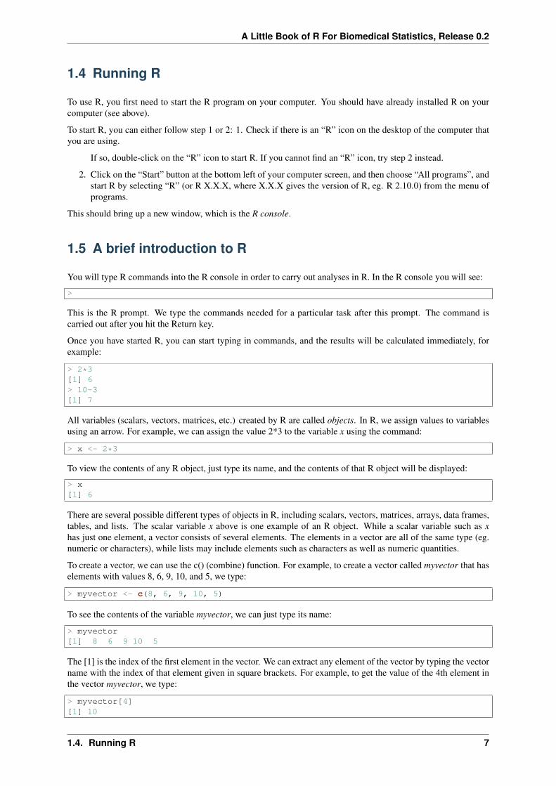
You will type R commands into the R console in order to carry out analyses in R. In the R console you will see:

>

This is the R prompt. We type the commands needed for a particular task after this prompt. The command iscarried out after you hit the Return key.

Once you have started R, you can start typing in commands, and the results will be calculated immediately, forexample:

> 2*3[1] 6> 10-3[1] 7

All variables (scalars, vectors, matrices, etc.) created by R are called objects. In R, we assign values to variablesusing an arrow. For example, we can assign the value 2*3 to the variable x using the command:

> x <- 2*3

To view the contents of any R object, just type its name, and the contents of that R object will be displayed:

> x[1] 6

There are several possible different types of objects in R, including scalars, vectors, matrices, arrays, data frames,tables, and lists. The scalar variable x above is one example of an R object. While a scalar variable such as xhas just one element, a vector consists of several elements. The elements in a vector are all of the same type (eg.numeric or characters), while lists may include elements such as characters as well as numeric quantities.

To create a vector, we can use the c() (combine) function. For example, to create a vector called myvector that haselements with values 8, 6, 9, 10, and 5, we type:

> myvector <- c(8, 6, 9, 10, 5)

To see the contents of the variable myvector, we can just type its name:

> myvector[1] 8 6 9 10 5

The [1] is the index of the first element in the vector. We can extract any element of the vector by typing the vectorname with the index of that element given in square brackets. For example, to get the value of the 4th element inthe vector myvector, we type:

> myvector[4][1] 10

1.4. Running R 7


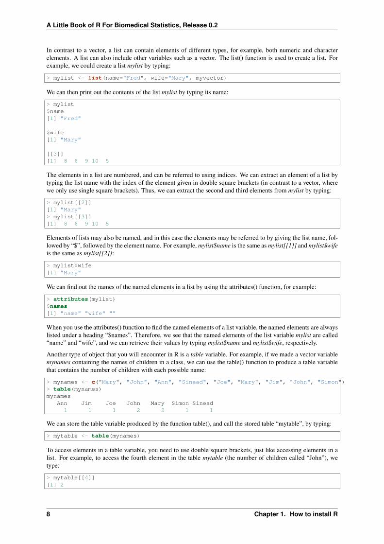
In contrast to a vector, a list can contain elements of different types, for example, both numeric and characterelements. A list can also include other variables such as a vector. The list() function is used to create a list. Forexample, we could create a list mylist by typing:

> mylist <- list(name="Fred", wife="Mary", myvector)

We can then print out the contents of the list mylist by typing its name:

> mylist$name[1] "Fred"

$wife[1] "Mary"

[[3]][1] 8 6 9 10 5

The elements in a list are numbered, and can be referred to using indices. We can extract an element of a list bytyping the list name with the index of the element given in double square brackets (in contrast to a vector, wherewe only use single square brackets). Thus, we can extract the second and third elements from mylist by typing:

> mylist[[2]][1] "Mary"> mylist[[3]][1] 8 6 9 10 5

Elements of lists may also be named, and in this case the elements may be referred to by giving the list name, fol-lowed by “$”, followed by the element name. For example, mylist$name is the same as mylist[[1]] and mylist$wifeis the same as mylist[[2]]:

> mylist$wife[1] "Mary"

We can find out the names of the named elements in a list by using the attributes() function, for example:

> attributes(mylist)$names[1] "name" "wife" ""

When you use the attributes() function to find the named elements of a list variable, the named elements are alwayslisted under a heading “$names”. Therefore, we see that the named elements of the list variable mylist are called“name” and “wife”, and we can retrieve their values by typing mylist$name and mylist$wife, respectively.

Another type of object that you will encounter in R is a table variable. For example, if we made a vector variablemynames containing the names of children in a class, we can use the table() function to produce a table variablethat contains the number of children with each possible name:

> mynames <- c("Mary", "John", "Ann", "Sinead", "Joe", "Mary", "Jim", "John", "Simon")> table(mynames)mynames

Ann Jim Joe John Mary Simon Sinead1 1 1 2 2 1 1

We can store the table variable produced by the function table(), and call the stored table “mytable”, by typing:

> mytable <- table(mynames)

To access elements in a table variable, you need to use double square brackets, just like accessing elements in alist. For example, to access the fourth element in the table mytable (the number of children called “John”), wetype:

> mytable[[4]][1] 2



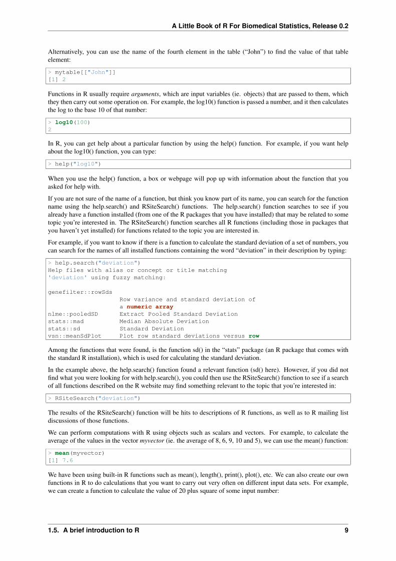
Alternatively, you can use the name of the fourth element in the table (“John”) to find the value of that tableelement:

> mytable[["John"]][1] 2

Functions in R usually require arguments, which are input variables (ie. objects) that are passed to them, whichthey then carry out some operation on. For example, the log10() function is passed a number, and it then calculatesthe log to the base 10 of that number:

> log10(100)2

In R, you can get help about a particular function by using the help() function. For example, if you want helpabout the log10() function, you can type:

> help("log10")

When you use the help() function, a box or webpage will pop up with information about the function that youasked for help with.

If you are not sure of the name of a function, but think you know part of its name, you can search for the functionname using the help.search() and RSiteSearch() functions. The help.search() function searches to see if youalready have a function installed (from one of the R packages that you have installed) that may be related to sometopic you’re interested in. The RSiteSearch() function searches all R functions (including those in packages thatyou haven’t yet installed) for functions related to the topic you are interested in.

For example, if you want to know if there is a function to calculate the standard deviation of a set of numbers, youcan search for the names of all installed functions containing the word “deviation” in their description by typing:

> help.search("deviation")Help files with alias or concept or title matching'deviation' using fuzzy matching:

genefilter::rowSdsRow variance and standard deviation ofa numeric array

nlme::pooledSD Extract Pooled Standard Deviationstats::mad Median Absolute Deviationstats::sd Standard Deviationvsn::meanSdPlot Plot row standard deviations versus row

Among the functions that were found, is the function sd() in the “stats” package (an R package that comes withthe standard R installation), which is used for calculating the standard deviation.

In the example above, the help.search() function found a relevant function (sd() here). However, if you did notfind what you were looking for with help.search(), you could then use the RSiteSearch() function to see if a searchof all functions described on the R website may find something relevant to the topic that you’re interested in:

> RSiteSearch("deviation")

The results of the RSiteSearch() function will be hits to descriptions of R functions, as well as to R mailing listdiscussions of those functions.

We can perform computations with R using objects such as scalars and vectors. For example, to calculate theaverage of the values in the vector myvector (ie. the average of 8, 6, 9, 10 and 5), we can use the mean() function:

> mean(myvector)[1] 7.6

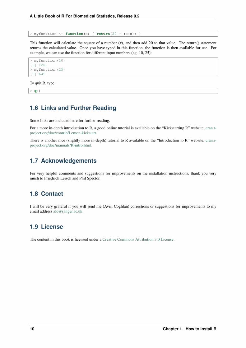
We have been using built-in R functions such as mean(), length(), print(), plot(), etc. We can also create our ownfunctions in R to do calculations that you want to carry out very often on different input data sets. For example,we can create a function to calculate the value of 20 plus square of some input number:

1.5. A brief introduction to R 9


> myfunction <- function(x) { return(20 + (x*x)) }

This function will calculate the square of a number (x), and then add 20 to that value. The return() statementreturns the calculated value. Once you have typed in this function, the function is then available for use. Forexample, we can use the function for different input numbers (eg. 10, 25):

> myfunction(10)[1] 120> myfunction(25)[1] 645

To quit R, type:

> q()

1.6 Links and Further Reading

Some links are included here for further reading.

For a more in-depth introduction to R, a good online tutorial is available on the “Kickstarting R” website, cran.r-project.org/doc/contrib/Lemon-kickstart.

There is another nice (slightly more in-depth) tutorial to R available on the “Introduction to R” website, cran.r-project.org/doc/manuals/R-intro.html.

1.7 Acknowledgements

For very helpful comments and suggestions for improvements on the installation instructions, thank you verymuch to Friedrich Leisch and Phil Spector.

1.8 Contact

I will be very grateful if you will send me (Avril Coghlan) corrections or suggestions for improvements to myemail address [email protected]

1.9 License

The content in this book is licensed under a Creative Commons Attribution 3.0 License.


http://cran.r-project.org/doc/contrib/Lemon-kickstart/


http://cran.r-project.org/doc/manuals/R-intro.html



http://creativecommons.org/licenses/by/3.0/

CHAPTER 2

Using R for Biomedical Statistics

2.1 Biomedical statistics

This booklet tells you how to use the R software to carry out some simple analyses that are common in biomedicalstatistics. In particular, the focus is on cohort and case-control studies that aim to test whether particular factorsare associated with disease, randomised trials, and meta-analysis.

This booklet assumes that the reader has some basic knowledge of biomedical statistics, and the principal focusof the booklet is not to explain biomedical statistics analyses, but rather to explain how to carry out these analysesusing R.

If you are new to biomedical statistics, and want to learn more about any of the concepts presented here, I wouldhighly recommend the Open University book “Medical Statistics” (product code M249/01), available from fromthe Open University Shop.

There is a pdf version of this booklet available at https://media.readthedocs.org/pdf/a-little-book-of-r-for-biomedical-statistics/latest/a-little-book-of-r-for-biomedical-statistics.pdf.

If you like this booklet, you may also like to check out my booklet on using R for time series analysis, http://a-little-book-of-r-for-time-series.readthedocs.org/ and my booklet on using R for multivariate analysis, http://little-book-of-r-for-multivariate-analysis.readthedocs.org/.

2.2 Calculating Relative Risks for a Cohort Study

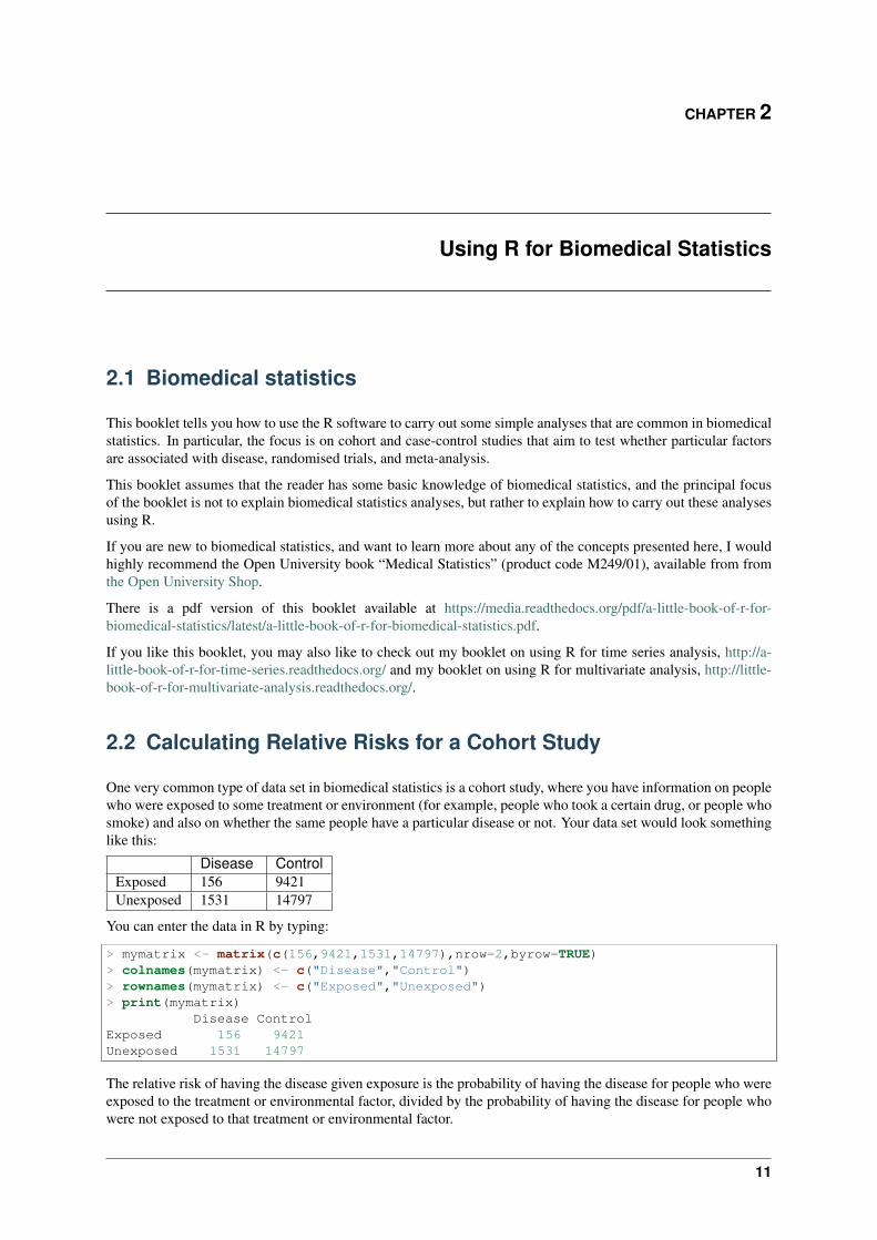
One very common type of data set in biomedical statistics is a cohort study, where you have information on peoplewho were exposed to some treatment or environment (for example, people who took a certain drug, or people whosmoke) and also on whether the same people have a particular disease or not. Your data set would look somethinglike this:

Disease ControlExposed 156 9421Unexposed 1531 14797

You can enter the data in R by typing:

> mymatrix <- matrix(c(156,9421,1531,14797),nrow=2,byrow=TRUE)> colnames(mymatrix) <- c("Disease","Control")> rownames(mymatrix) <- c("Exposed","Unexposed")> print(mymatrix)


The relative risk of having the disease given exposure is the probability of having the disease for people who wereexposed to the treatment or environmental factor, divided by the probability of having the disease for people whowere not exposed to that treatment or environmental factor.

11

http://www.ouw.co.uk/store/








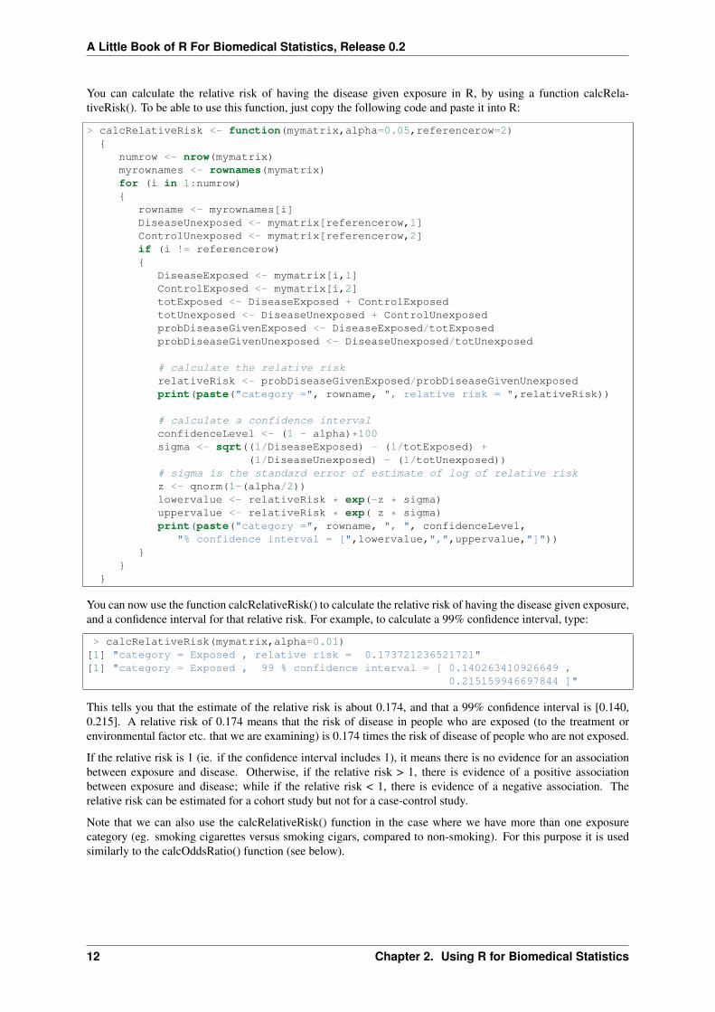
You can calculate the relative risk of having the disease given exposure in R, by using a function calcRela-tiveRisk(). To be able to use this function, just copy the following code and paste it into R:

> calcRelativeRisk <- function(mymatrix,alpha=0.05,referencerow=2){

numrow <- nrow(mymatrix)myrownames <- rownames(mymatrix)for (i in 1:numrow){

rowname <- myrownames[i]DiseaseUnexposed <- mymatrix[referencerow,1]ControlUnexposed <- mymatrix[referencerow,2]if (i != referencerow){

DiseaseExposed <- mymatrix[i,1]ControlExposed <- mymatrix[i,2]totExposed <- DiseaseExposed + ControlExposedtotUnexposed <- DiseaseUnexposed + ControlUnexposedprobDiseaseGivenExposed <- DiseaseExposed/totExposedprobDiseaseGivenUnexposed <- DiseaseUnexposed/totUnexposed

# calculate the relative riskrelativeRisk <- probDiseaseGivenExposed/probDiseaseGivenUnexposedprint(paste("category =", rowname, ", relative risk = ",relativeRisk))

# calculate a confidence intervalconfidenceLevel <- (1 - alpha)*100sigma <- sqrt((1/DiseaseExposed) - (1/totExposed) +

(1/DiseaseUnexposed) - (1/totUnexposed))# sigma is the standard error of estimate of log of relative riskz <- qnorm(1-(alpha/2))lowervalue <- relativeRisk * exp(-z * sigma)uppervalue <- relativeRisk * exp( z * sigma)print(paste("category =", rowname, ", ", confidenceLevel,

"% confidence interval = [",lowervalue,",",uppervalue,"]"))}

}}

You can now use the function calcRelativeRisk() to calculate the relative risk of having the disease given exposure,and a confidence interval for that relative risk. For example, to calculate a 99% confidence interval, type:

> calcRelativeRisk(mymatrix,alpha=0.01)[1] "category = Exposed , relative risk = 0.173721236521721"[1] "category = Exposed , 99 % confidence interval = [ 0.140263410926649 ,

0.215159946697844 ]"

This tells you that the estimate of the relative risk is about 0.174, and that a 99% confidence interval is [0.140,0.215]. A relative risk of 0.174 means that the risk of disease in people who are exposed (to the treatment orenvironmental factor etc. that we are examining) is 0.174 times the risk of disease of people who are not exposed.

If the relative risk is 1 (ie. if the confidence interval includes 1), it means there is no evidence for an associationbetween exposure and disease. Otherwise, if the relative risk > 1, there is evidence of a positive associationbetween exposure and disease; while if the relative risk < 1, there is evidence of a negative association. Therelative risk can be estimated for a cohort study but not for a case-control study.

Note that we can also use the calcRelativeRisk() function in the case where we have more than one exposurecategory (eg. smoking cigarettes versus smoking cigars, compared to non-smoking). For this purpose it is usedsimilarly to the calcOddsRatio() function (see below).

12 Chapter 2. Using R for Biomedical Statistics


2.3 Calculating Odds Ratios for a Cohort or Case-Control Study

As well as the relative risk of disease given exposure (to some treatment or environmental factor eg. smoking orsome drug), you can also calculate the odds ratio for association between the exposure and the disease in a cohortstudy. The odds ratio is also commonly calculated in a case-control study.

The odds ratio for association between the exposure and the disease is the ratio of: (i) the probability of havingthe disease for people who were exposed to the treatment or environmental factor, divided by the probability ofnot having the disease for people who were exposed, and (ii) the probability of having the disease for people whowere not exposed to the treatment or environmental factor, divided by the probability of not having the disease forpeople who were not exposed.

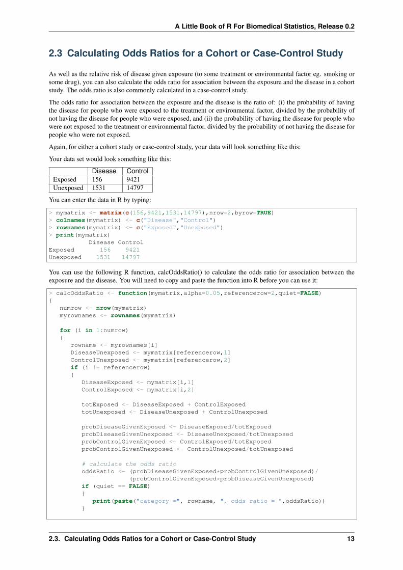
Again, for either a cohort study or case-control study, your data will look something like this:

Your data set would look something like this:


You can enter the data in R by typing:

> mymatrix <- matrix(c(156,9421,1531,14797),nrow=2,byrow=TRUE)> colnames(mymatrix) <- c("Disease","Control")> rownames(mymatrix) <- c("Exposed","Unexposed")> print(mymatrix)


You can use the following R function, calcOddsRatio() to calculate the odds ratio for association between theexposure and the disease. You will need to copy and paste the function into R before you can use it:

> calcOddsRatio <- function(mymatrix,alpha=0.05,referencerow=2,quiet=FALSE){

numrow <- nrow(mymatrix)myrownames <- rownames(mymatrix)

for (i in 1:numrow){

rowname <- myrownames[i]DiseaseUnexposed <- mymatrix[referencerow,1]ControlUnexposed <- mymatrix[referencerow,2]if (i != referencerow){

DiseaseExposed <- mymatrix[i,1]ControlExposed <- mymatrix[i,2]

totExposed <- DiseaseExposed + ControlExposedtotUnexposed <- DiseaseUnexposed + ControlUnexposed

probDiseaseGivenExposed <- DiseaseExposed/totExposedprobDiseaseGivenUnexposed <- DiseaseUnexposed/totUnexposedprobControlGivenExposed <- ControlExposed/totExposedprobControlGivenUnexposed <- ControlUnexposed/totUnexposed

# calculate the odds ratiooddsRatio <- (probDiseaseGivenExposed*probControlGivenUnexposed)/

(probControlGivenExposed*probDiseaseGivenUnexposed)if (quiet == FALSE){

print(paste("category =", rowname, ", odds ratio = ",oddsRatio))}

2.3. Calculating Odds Ratios for a Cohort or Case-Control Study 13


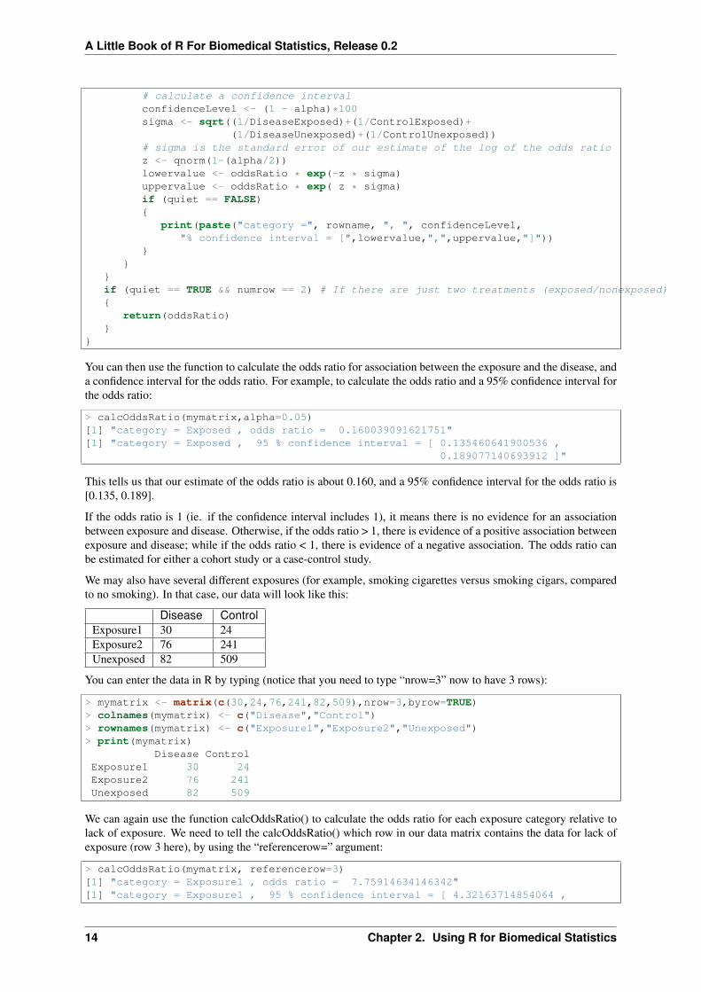
# calculate a confidence intervalconfidenceLevel <- (1 - alpha)*100sigma <- sqrt((1/DiseaseExposed)+(1/ControlExposed)+

(1/DiseaseUnexposed)+(1/ControlUnexposed))# sigma is the standard error of our estimate of the log of the odds ratioz <- qnorm(1-(alpha/2))lowervalue <- oddsRatio * exp(-z * sigma)uppervalue <- oddsRatio * exp( z * sigma)if (quiet == FALSE){

print(paste("category =", rowname, ", ", confidenceLevel,"% confidence interval = [",lowervalue,",",uppervalue,"]"))

}}

}if (quiet == TRUE && numrow == 2) # If there are just two treatments (exposed/nonexposed){

return(oddsRatio)}

}

You can then use the function to calculate the odds ratio for association between the exposure and the disease, anda confidence interval for the odds ratio. For example, to calculate the odds ratio and a 95% confidence interval forthe odds ratio:

> calcOddsRatio(mymatrix,alpha=0.05)[1] "category = Exposed , odds ratio = 0.160039091621751"[1] "category = Exposed , 95 % confidence interval = [ 0.135460641900536 ,

0.189077140693912 ]"

This tells us that our estimate of the odds ratio is about 0.160, and a 95% confidence interval for the odds ratio is[0.135, 0.189].

If the odds ratio is 1 (ie. if the confidence interval includes 1), it means there is no evidence for an associationbetween exposure and disease. Otherwise, if the odds ratio > 1, there is evidence of a positive association betweenexposure and disease; while if the odds ratio < 1, there is evidence of a negative association. The odds ratio canbe estimated for either a cohort study or a case-control study.

We may also have several different exposures (for example, smoking cigarettes versus smoking cigars, comparedto no smoking). In that case, our data will look like this:

Disease ControlExposure1 30 24Exposure2 76 241Unexposed 82 509

You can enter the data in R by typing (notice that you need to type “nrow=3” now to have 3 rows):

> mymatrix <- matrix(c(30,24,76,241,82,509),nrow=3,byrow=TRUE)> colnames(mymatrix) <- c("Disease","Control")> rownames(mymatrix) <- c("Exposure1","Exposure2","Unexposed")> print(mymatrix)

Disease ControlExposure1 30 24Exposure2 76 241Unexposed 82 509

We can again use the function calcOddsRatio() to calculate the odds ratio for each exposure category relative tolack of exposure. We need to tell the calcOddsRatio() which row in our data matrix contains the data for lack ofexposure (row 3 here), by using the “referencerow=” argument:

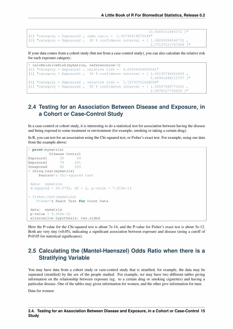
> calcOddsRatio(mymatrix, referencerow=3)[1] "category = Exposure1 , odds ratio = 7.75914634146342"[1] "category = Exposure1 , 95 % confidence interval = [ 4.32163714854064 ,



13.9309131884372 ]"[1] "category = Exposure2 , odds ratio = 1.95749418075094"[1] "category = Exposure2 , 95 % confidence interval = [ 1.38263094540732 ,

2.77137111707344 ]"

If your data comes from a cohort study (but not from a case-control study), you can also calculate the relative riskfor each exposure category:

> calcRelativeRisk(mymatrix, referencerow=3)[1] "category = Exposure1 , relative risk = 4.00406504065041"[1] "category = Exposure1 , 95 % confidence interval = [ 2.93130744422409 ,

5.46941498113737 ]"[1] "category = Exposure2 , relative risk = 1.72793721628068"[1] "category = Exposure2 , 95 % confidence interval = [ 1.30507489771431 ,

2.2878127750653 ]"

2.4 Testing for an Association Between Disease and Exposure, ina Cohort or Case-Control Study

In a case-control or cohort study, it is interesting to do a statistical test for association between having the diseaseand being exposed to some treatment or environment (for example, smoking or taking a certain drug).

In R, you can test for an association using the Chi-squared test, or Fisher’s exact test. For example, using our datafrom the example above:

> print(mymatrix)Disease Control

Exposure1 30 24Exposure2 76 241Unexposed 82 509> chisq.test(mymatrix)

Pearson's Chi-squared test

data: mymatrixX-squared = 60.5762, df = 2, p-value = 7.015e-14

> fisher.test(mymatrix)Fisher's Exact Test for Count Data

data: mymatrixp-value = 5.263e-12alternative hypothesis: two.sided

Here the P-value for the Chi-squared test is about 7e-14, and the P-value for Fisher’s exact test is about 5e-12.Both are very tiny (<0.05), indicating a significant association between exposure and disease (using a cutoff ofP<0.05 for statistical significance).

2.5 Calculating the (Mantel-Haenszel) Odds Ratio when there is aStratifying Variable

You may have data from a cohort study or case-control study that is stratified, for example, the data may beseparated (stratified) by the sex of the people studied. For example, we may have two different tables givinginformation on the relationship between exposure (eg. to a certain drug or smoking cigarettes) and having aparticular disease. One of the tables may given information for women, and the other give information for men.

Data for women:

2.4. Testing for an Association Between Disease and Exposure, in a Cohort or Case-ControlStudy

15


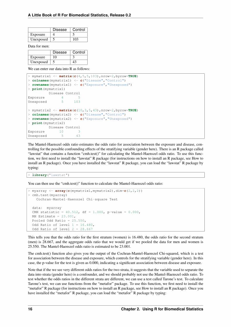
Disease ControlExposure 4 5Unexposed 5 103

Data for men:


We can enter our data into R as follows:

> mymatrix1 <- matrix(c(4,5,5,103),nrow=2,byrow=TRUE)> colnames(mymatrix1) <- c("Disease","Control")> rownames(mymatrix1) <- c("Exposure","Unexposed")> print(mymatrix1)


> mymatrix2 <- matrix(c(10,3,5,43),nrow=2,byrow=TRUE)> colnames(mymatrix2) <- c("Disease","Control")> rownames(mymatrix2) <- c("Exposure","Unexposed")> print(mymatrix2)


The Mantel-Haenszel odds ratio estimates the odds ratio for association between the exposure and disease, con-trolling for the possible confounding effects of the stratifying variable (gender here). There is an R package called“lawstat” that contains a function “cmh.test()” for calculating the Mantel-Haenszel odds ratio. To use this func-tion, we first need to install the “lawstat” R package (for instructions on how to install an R package, see How toinstall an R package). Once you have installed the “lawstat” R package, you can load the “lawstat” R package bytyping:

> library("lawstat")

You can then use the “cmh.test()” function to calculate the Mantel-Haenszel odds ratio:

> myarray <- array(c(mymatrix1,mymatrix2),dim=c(2,2,2))> cmh.test(myarray)

Cochran-Mantel-Haenszel Chi-square Test

data: myarrayCMH statistic = 40.512, df = 1.000, p-value = 0.000,MH Estimate = 23.001,Pooled Odd Ratio = 25.550,Odd Ratio of level 1 = 16.480,Odd Ratio of level 2 = 28.667

This tells you that the odds ratio for the first stratum (women) is 16.480, the odds ratio for the second stratum(men) is 28.667, and the aggregate odds ratio that we would get if we pooled the data for men and women is25.550. The Mantel-Haenszel odds ratio is estimated to be 23.001.

The cmh.test() function also gives you the output of the Cochran-Mantel-Haenszel Chi-squared, which is a testfor association between the disease and exposure, which controls for the stratifying variable (gender here). In thiscase, the p-value for the test is given as 0.000, indicating a significant association between disease and exposure.

Note that if the we see very different odds ratios for the two strata, it suggests that the variable used to separate thedata into strata (gender here) is a confounder, and we should probably not use the Mantel-Haenszel odds ratio. Totest whether the odds ratios in the different strata are different, we can use a test called Tarone’s test. To calculateTarone’s test, we can use functions from the “metafor” package. To use this function, we first need to install the“metafor” R package (for instructions on how to install an R package, see How to install an R package). Once youhave installed the “metafor” R package, you can load the “metafor” R package by typing:



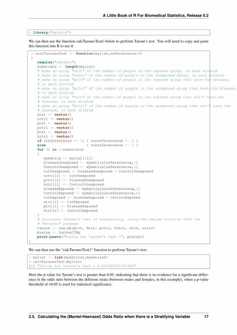
> library("metafor")

We can then use the function calcTaronesTest() below to perform Tarone’s test. You will need to copy and pastethis function into R to use it:

> calcTaronesTest <- function(mylist,referencerow=2){

require("metafor")numstrata <- length(mylist)# make an array "ntrt" of the number of people in the exposed group, in each stratum# make an array "nctrl" of the number of people in the unexposed group, in each stratum# make an array "ptrt" of the number of people in the exposed group that have the disease,# in each stratum# make an array "pctrl" of the number of people in the unexposed group that have the disease,# in each stratum# make an array "htrt" of the number of people in the exposed group that don't have the# disease, in each stratum# make an array "hctrl" of the number of people in the unexposed group that don't have the# disease, in each stratumntrt <- vector()nctrl <- vector()ptrt <- vector()pctrl <- vector()htrt <- vector()hctrl <- vector()if (referencerow == 1) { nonreferencerow <- 2 }else { nonreferencerow <- 1 }for (i in 1:numstrata){

mymatrix <- mylist[[i]]DiseaseUnexposed <- mymatrix[referencerow,1]ControlUnexposed <- mymatrix[referencerow,2]totUnexposed <- DiseaseUnexposed + ControlUnexposednctrl[i] <- totUnexposedpctrl[i] <- DiseaseUnexposedhctrl[i] <- ControlUnexposedDiseaseExposed <- mymatrix[nonreferencerow,1]ControlExposed <- mymatrix[nonreferencerow,2]totExposed <- DiseaseExposed + ControlExposedntrt[i] <- totExposedptrt[i] <- DiseaseExposedhtrt[i] <- ControlExposed

}# calculate Tarone's test of homogeneity, using the rma.mh function from the# "metafor" packagetarone <- rma.mh(ptrt, htrt, pctrl, hctrl, ntrt, nctrl)pvalue <- tarone$TApprint(paste("Pvalue for Tarone's test =", pvalue))

}

We can then use the “calcTaronesTest()” function to perform Tarone’s test:

> mylist <- list(mymatrix1,mymatrix2)> calcTaronesTest(mylist)[1] "Pvalue for Tarone's test = 0.627420741721689"

Here the p-value for Tarone’s test is greater than 0.05, indicating that there is no evidence for a significant differ-ence in the odds ratio between the different strata (between males and females, in this example), when a p-valuethreshold of <0.05 is used for statistical significance.

2.5. Calculating the (Mantel-Haenszel) Odds Ratio when there is a Stratifying Variable 17


2.6 Testing for an Association Between Exposure and Disease in aMatched Case-Control Study

In a 1-1 matched case-control study, there is a control individual who is matched to each person who has thedisease. The matched control individual has the same age, race, sex, etc. as the person who has the disease. Thenwe look to see whether the control individuals and individuals with the disease were exposed to some factor (eg.if they smoked, or took a certain drug). The data would look something like this:

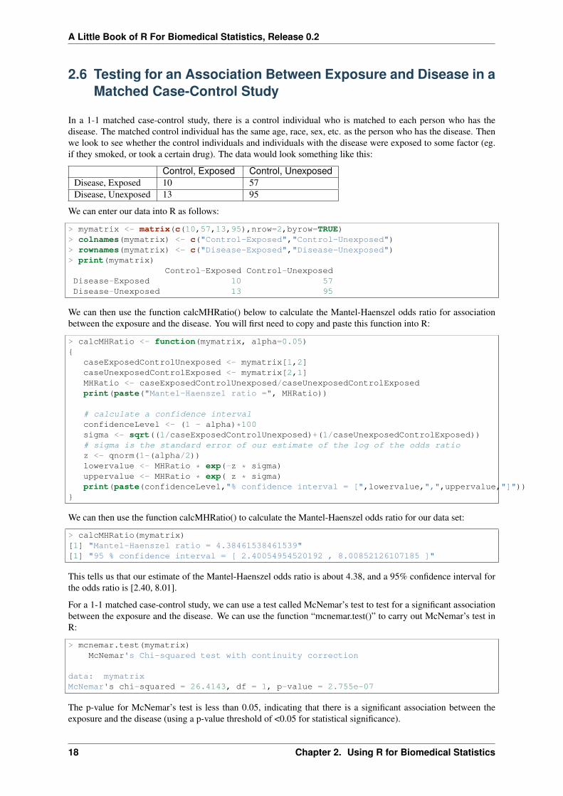
Control, Exposed Control, UnexposedDisease, Exposed 10 57Disease, Unexposed 13 95

We can enter our data into R as follows:

> mymatrix <- matrix(c(10,57,13,95),nrow=2,byrow=TRUE)> colnames(mymatrix) <- c("Control-Exposed","Control-Unexposed")> rownames(mymatrix) <- c("Disease-Exposed","Disease-Unexposed")> print(mymatrix)

Control-Exposed Control-UnexposedDisease-Exposed 10 57Disease-Unexposed 13 95

We can then use the function calcMHRatio() below to calculate the Mantel-Haenszel odds ratio for associationbetween the exposure and the disease. You will first need to copy and paste this function into R:

> calcMHRatio <- function(mymatrix, alpha=0.05){

caseExposedControlUnexposed <- mymatrix[1,2]caseUnexposedControlExposed <- mymatrix[2,1]MHRatio <- caseExposedControlUnexposed/caseUnexposedControlExposedprint(paste("Mantel-Haenszel ratio =", MHRatio))

# calculate a confidence intervalconfidenceLevel <- (1 - alpha)*100sigma <- sqrt((1/caseExposedControlUnexposed)+(1/caseUnexposedControlExposed))# sigma is the standard error of our estimate of the log of the odds ratioz <- qnorm(1-(alpha/2))lowervalue <- MHRatio * exp(-z * sigma)uppervalue <- MHRatio * exp( z * sigma)print(paste(confidenceLevel,"% confidence interval = [",lowervalue,",",uppervalue,"]"))

}

We can then use the function calcMHRatio() to calculate the Mantel-Haenszel odds ratio for our data set:

> calcMHRatio(mymatrix)[1] "Mantel-Haenszel ratio = 4.38461538461539"[1] "95 % confidence interval = [ 2.40054954520192 , 8.00852126107185 ]"

This tells us that our estimate of the Mantel-Haenszel odds ratio is about 4.38, and a 95% confidence interval forthe odds ratio is [2.40, 8.01].

For a 1-1 matched case-control study, we can use a test called McNemar’s test to test for a significant associationbetween the exposure and the disease. We can use the function “mcnemar.test()” to carry out McNemar’s test inR:

> mcnemar.test(mymatrix)McNemar's Chi-squared test with continuity correction

data: mymatrixMcNemar's chi-squared = 26.4143, df = 1, p-value = 2.755e-07

The p-value for McNemar’s test is less than 0.05, indicating that there is a significant association between theexposure and the disease (using a p-value threshold of <0.05 for statistical significance).



2.7 Dose-response analysis:

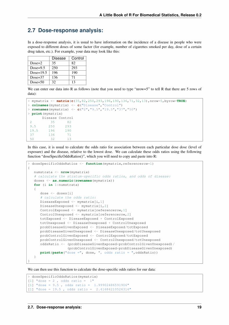
In a dose-response analysis, it is usual to have information on the incidence of a disease in people who wereexposed to different doses of some factor (for example, number of cigarettes smoked per day, dose of a certaindrug taken, etc.). For example, your data may look like this:

Disease ControlDose=2 35 82Dose=9.5 250 293Dose=19.5 196 190Dose=37 136 71Dose=50 32 13

We can enter our data into R as follows (note that you need to type “nrow=5” to tell R that there are 5 rows ofdata):

> mymatrix <- matrix(c(35,82,250,293,196,190,136,71,32,13),nrow=5,byrow=TRUE)> colnames(mymatrix) <- c("Disease","Control")> rownames(mymatrix) <- c("2","9.5","19.5","37","50")> print(mymatrix)

Disease Control2 35 829.5 250 29319.5 196 19037 136 7150 32 13

In this case, it is usual to calculate the odds ratio for association between each particular dose dose (level ofexposure) and the disease, relative to the lowest dose. We can calculate these odds ratios using the followingfunction “doseSpecificOddsRatios()”, which you will need to copy and paste into R:

> doseSpecificOddsRatios <- function(mymatrix,referencerow=1){

numstrata <- nrow(mymatrix)# calculate the stratum-specific odds ratios, and odds of disease:doses <- as.numeric(rownames(mymatrix))for (i in 1:numstrata){

dose <- doses[i]# calculate the odds ratio:DiseaseExposed <- mymatrix[i,1]DiseaseUnexposed <- mymatrix[i,2]ControlExposed <- mymatrix[referencerow,1]ControlUnexposed <- mymatrix[referencerow,2]totExposed <- DiseaseExposed + ControlExposedtotUnexposed <- DiseaseUnexposed + ControlUnexposedprobDiseaseGivenExposed <- DiseaseExposed/totExposedprobDiseaseGivenUnexposed <- DiseaseUnexposed/totUnexposedprobControlGivenExposed <- ControlExposed/totExposedprobControlGivenUnexposed <- ControlUnexposed/totUnexposedoddsRatio <- (probDiseaseGivenExposed*probControlGivenUnexposed)/

(probControlGivenExposed*probDiseaseGivenUnexposed)print(paste("dose =", dose, ", odds ratio = ",oddsRatio))

}}

We can then use this function to calculate the dose-specific odds ratios for our data:

> doseSpecificOddsRatios(mymatrix)[1] "dose = 2 , odds ratio = 1"[1] "dose = 9.5 , odds ratio = 1.99902486591906"[1] "dose = 19.5 , odds ratio = 2.41684210526316"

2.7. Dose-response analysis: 19


[1] "dose = 37 , odds ratio = 4.48772635814889"[1] "dose = 50 , odds ratio = 5.76703296703297"

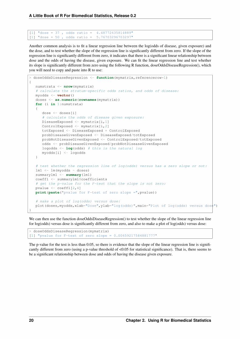
Another common analysis is to fit a linear regression line between the log(odds of disease, given exposure) andthe dose, and to test whether the slope of the regression line is significantly different from zero. If the slope of theregression line is significantly different from zero, it indicates that there is a significant linear relationship betweendose and the odds of having the disease, given exposure. We can fit the linear regression line and test whetherits slope is significantly different from zero using the following R function, doseOddsDiseaseRegression(), whichyou will need to copy and paste into R to use:

> doseOddsDiseaseRegression <- function(mymatrix,referencerow=1){

numstrata <- nrow(mymatrix)# calculate the stratum-specific odds ratios, and odds of disease:myodds <- vector()doses <- as.numeric(rownames(mymatrix))for (i in 1:numstrata){

dose <- doses[i]# calculate the odds of disease given exposure:DiseaseExposed <- mymatrix[i,1]ControlExposed <- mymatrix[i,2]totExposed <- DiseaseExposed + ControlExposedprobDiseaseGivenExposed <- DiseaseExposed/totExposedprobNotDiseaseGivenExposed <- ControlExposed/totExposedodds <- probDiseaseGivenExposed/probNotDiseaseGivenExposedlogodds <- log(odds) # this is the natural logmyodds[i] <- logodds

}

# test whether the regression line of log(odds) versus has a zero slope or not:lm1 <- lm(myodds ~ doses)summarylm1 <- summary(lm1)coeff1 <- summarylm1$coefficients# get the p-value for the F-test that the slope is not zero:pvalue <- coeff1[2,4]print(paste("pvalue for F-test of zero slope =",pvalue))

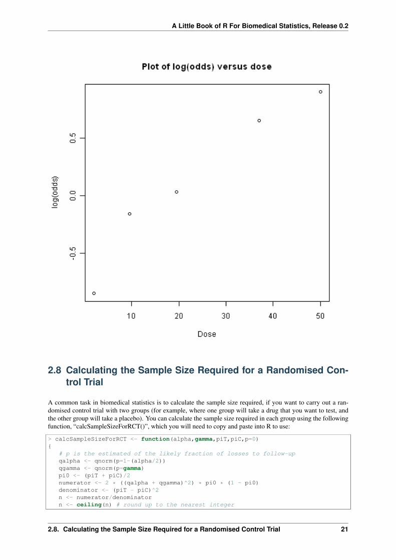
# make a plot of log(odds) versus dose:plot(doses,myodds,xlab="Dose",ylab="log(odds)",main="Plot of log(odds) versus dose")

}

We can then use the function doseOddsDiseaseRegression() to test whether the slope of the linear regression linefor log(odds) versus dose is significantly different from zero, and also to make a plot of log(odds) versus dose:

> doseOddsDiseaseRegression(mymatrix)[1] "pvalue for F-test of zero slope = 0.00659217584881777"

The p-value for the test is less than 0.05, so there is evidence that the slope of the linear regression line is signifi-cantly different from zero (using a p-value threshold of <0.05 for statistical significance). That is, there seems tobe a significant relationship between dose and odds of having the disease given exposure.



2.8 Calculating the Sample Size Required for a Randomised Con-trol Trial

A common task in biomedical statistics is to calculate the sample size required, if you want to carry out a ran-domised control trial with two groups (for example, where one group will take a drug that you want to test, andthe other group will take a placebo). You can calculate the sample size required in each group using the followingfunction, “calcSampleSizeForRCT()”, which you will need to copy and paste into R to use:

> calcSampleSizeForRCT <- function(alpha,gamma,piT,piC,p=0){

# p is the estimated of the likely fraction of losses to follow-upqalpha <- qnorm(p=1-(alpha/2))qgamma <- qnorm(p=gamma)pi0 <- (piT + piC)/2numerator <- 2 * ((qalpha + qgamma)^2) * pi0 * (1 - pi0)denominator <- (piT - piC)^2n <- numerator/denominatorn <- ceiling(n) # round up to the nearest integer

2.8. Calculating the Sample Size Required for a Randomised Control Trial 21


# adjust for likely losses to folow-upn <- n/(1-p)n <- ceiling(n) # round up to the nearest integerprint(paste("Sample size for each trial group = ",n))

}

To use the “calcSampleSizeForRCT()” function, you need to specify the significance level that you want to have,the power that you want to have, the estimated incidence of the disease in the control group (the group takinga placebo), and the estimated incidence of the disease in the treatment group (the group taking the drug). Forexample, if you want to have a 5% significance level and 90% power, and the estimated incidences of the diseasein the control and study groups is 0.20 and 0.15, respectively, then to calculate the required sample size for eachgroup, you would type:

> calcSampleSizeForRCT(alpha=0.05, gamma=0.90, piT=0.15, piC=0.2)[1] "Sample size for each trial group = 1214"

This tells us that the sample size required in each group is 1214 people, so overall we need 1214*2=2428 peoplein the randomised control trial.

If we estimate that there are likely to be a certain fraction of people who are lost to follow-up, we can adjust ourestimates of the number of people required for the trial. For example, if we estimate that 10% of the people arelikely to be lost to follow-up, we can calculate the number of people required for the trial as:

> calcSampleSizeForRCT(alpha=0.05, gamma=0.90, piT=0.15, piC=0.2, p=0.1)[1] "Sample size for each trial group = 1349"

This tells us that, if 10% of people are likely to be lost to follow-up, we need to have 1349 people in each groupin our trial, so 1349*2=2698 people overall.

2.9 Calculating the Power of a Randomised Control Trial

If, for practical reasons, you can only have a maximum of a certain number of people in each group of yourrandomised control trial, then you can calculate the statistical power that your trial will have. You can do thisusing the following function, “calcPowerForRC()”:

> calcPowerForRCT <- function(alpha,piT,piC,n){

qalpha <- qnorm(p=1-(alpha/2))pi0 <- (piT + piC)/2denominator <- 2 * pi0 * (1 - pi0)fraction <- n/denominatorqgamma <- (abs(piT - piC) * sqrt(fraction)) - qalphagamma <- pnorm(qgamma)print(paste("Power for the randomised controlled trial = ",gamma))

}

For example, to calculate the power of a randomised control trial involving 500 children (250 in the control groupand 250 in the treatment group), where the significance level is 0.05, and the estimated incidence of the disease inthe control and treatment group is 0.3 and 0.2, respectively, we type:

> calcPowerForRCT(alpha=0.05, piT=0.2, piC=0.3, n=250)[1] "Power for the randomised controlled trial = 0.73303725668939"

This tells us that the power for the randomised control trial will be 73%.



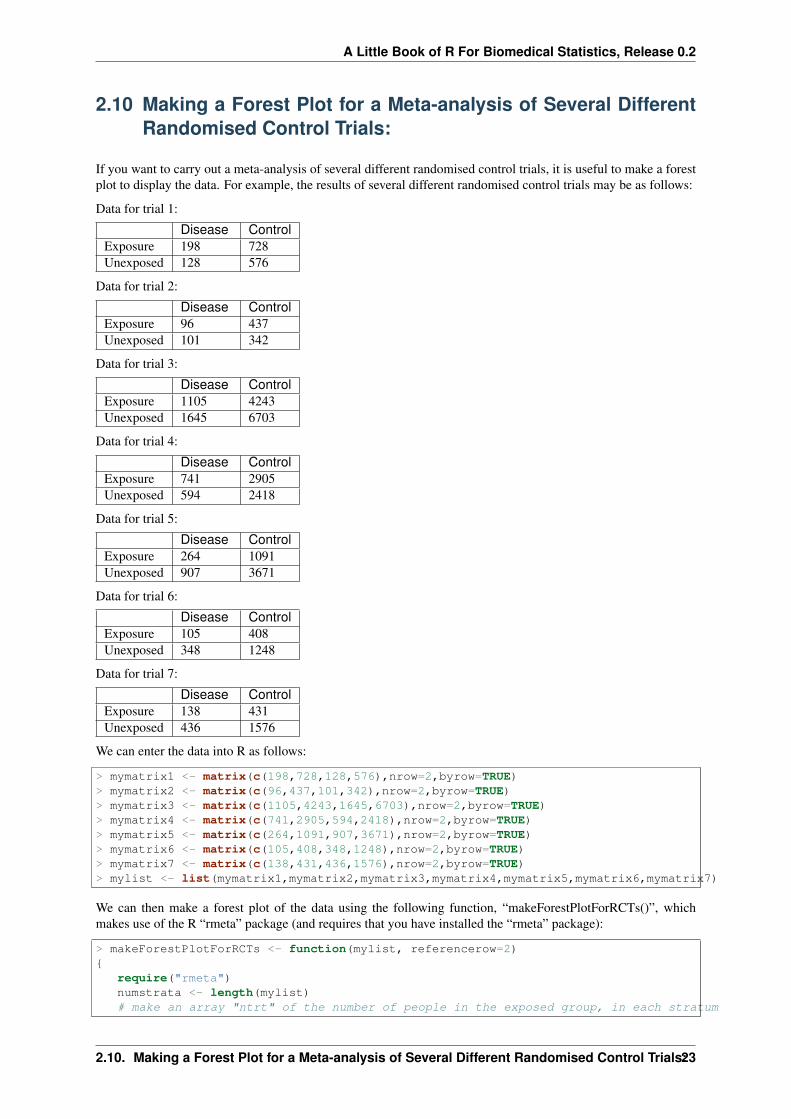
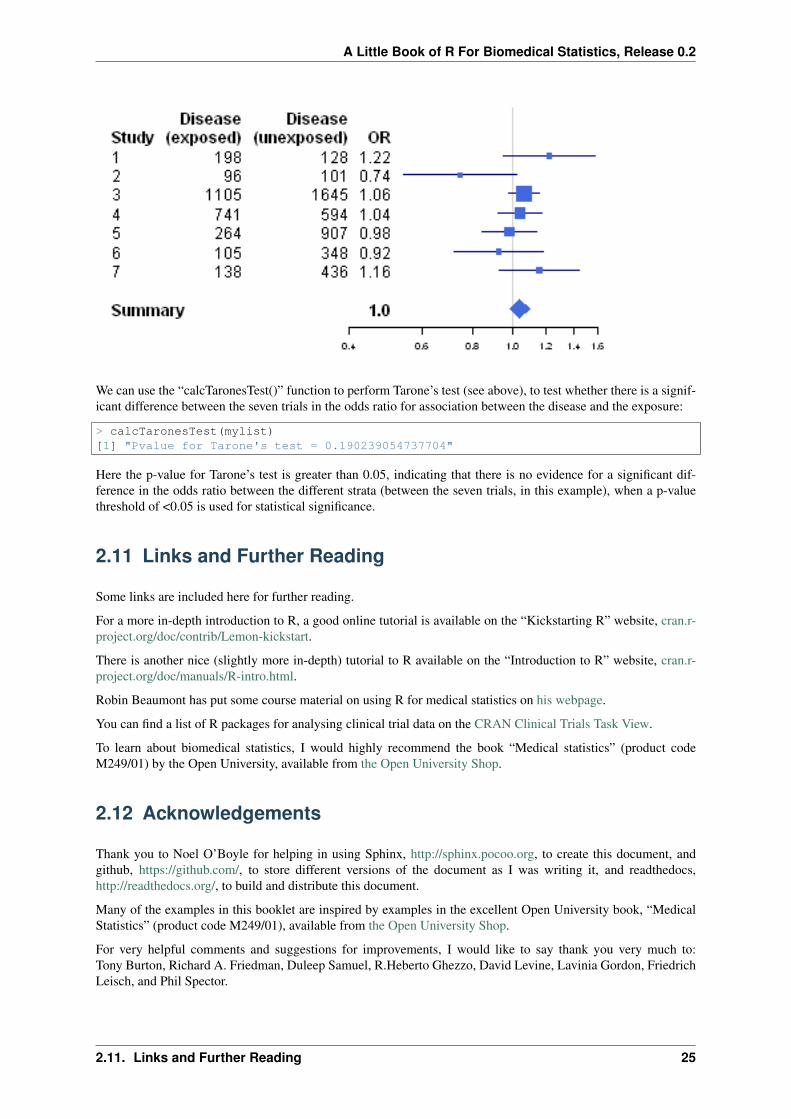
2.10 Making a Forest Plot for a Meta-analysis of Several DifferentRandomised Control Trials:

If you want to carry out a meta-analysis of several different randomised control trials, it is useful to make a forestplot to display the data. For example, the results of several different randomised control trials may be as follows:

Data for trial 1:


Data for trial 2:


Data for trial 3:


Data for trial 4:


Data for trial 5:


Data for trial 6:


Data for trial 7:


We can enter the data into R as follows:

> mymatrix1 <- matrix(c(198,728,128,576),nrow=2,byrow=TRUE)> mymatrix2 <- matrix(c(96,437,101,342),nrow=2,byrow=TRUE)> mymatrix3 <- matrix(c(1105,4243,1645,6703),nrow=2,byrow=TRUE)> mymatrix4 <- matrix(c(741,2905,594,2418),nrow=2,byrow=TRUE)> mymatrix5 <- matrix(c(264,1091,907,3671),nrow=2,byrow=TRUE)> mymatrix6 <- matrix(c(105,408,348,1248),nrow=2,byrow=TRUE)> mymatrix7 <- matrix(c(138,431,436,1576),nrow=2,byrow=TRUE)> mylist <- list(mymatrix1,mymatrix2,mymatrix3,mymatrix4,mymatrix5,mymatrix6,mymatrix7)

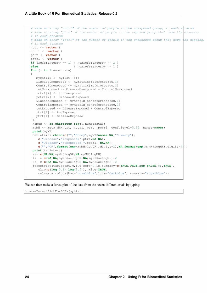
We can then make a forest plot of the data using the following function, “makeForestPlotForRCTs()”, whichmakes use of the R “rmeta” package (and requires that you have installed the “rmeta” package):

> makeForestPlotForRCTs <- function(mylist, referencerow=2){

require("rmeta")numstrata <- length(mylist)# make an array "ntrt" of the number of people in the exposed group, in each stratum

2.10. Making a Forest Plot for a Meta-analysis of Several Different Randomised Control Trials:23


# make an array "nctrl" of the number of people in the unexposed group, in each stratum# make an array "ptrt" of the number of people in the exposed group that have the disease,# in each stratum# make an array "pctrl" of the number of people in the unexposed group that have the disease,# in each stratumntrt <- vector()nctrl <- vector()ptrt <- vector()pctrl <- vector()if (referencerow == 1) { nonreferencerow <- 2 }else { nonreferencerow <- 1 }for (i in 1:numstrata){

mymatrix <- mylist[[i]]DiseaseUnexposed <- mymatrix[referencerow,1]ControlUnexposed <- mymatrix[referencerow,2]totUnexposed <- DiseaseUnexposed + ControlUnexposednctrl[i] <- totUnexposedpctrl[i] <- DiseaseUnexposedDiseaseExposed <- mymatrix[nonreferencerow,1]ControlExposed <- mymatrix[nonreferencerow,2]totExposed <- DiseaseExposed + ControlExposedntrt[i] <- totExposedptrt[i] <- DiseaseExposed

}names <- as.character(seq(1,numstrata))myMH <- meta.MH(ntrt, nctrl, ptrt, pctrl, conf.level=0.95, names=names)print(myMH)tabletext<-cbind(c("","Study",myMH$names,NA,"Summary"),

c("Disease","(exposed)",ptrt,NA,NA),c("Disease","(unexposed)",pctrl, NA,NA),c("","OR",format(exp(myMH$logOR),digits=2),NA,format(exp(myMH$logMH),digits=2)))

print(tabletext)m<- c(NA,NA,myMH$logOR,NA,myMH$logMH)l<- m-c(NA,NA,myMH$selogOR,NA,myMH$selogMH)*2u<- m+c(NA,NA,myMH$selogOR,NA,myMH$selogMH)*2forestplot(tabletext,m,l,u,zero=0,is.summary=c(TRUE,TRUE,rep(FALSE,8),TRUE),

clip=c(log(0.1),log(2.5)), xlog=TRUE,col=meta.colors(box="royalblue",line="darkblue", summary="royalblue"))

}

We can then make a forest plot of the data from the seven different trials by typing:

> makeForestPlotForRCTs(mylist)



We can use the “calcTaronesTest()” function to perform Tarone’s test (see above), to test whether there is a signif-icant difference between the seven trials in the odds ratio for association between the disease and the exposure:

> calcTaronesTest(mylist)[1] "Pvalue for Tarone's test = 0.190239054737704"

Here the p-value for Tarone’s test is greater than 0.05, indicating that there is no evidence for a significant dif-ference in the odds ratio between the different strata (between the seven trials, in this example), when a p-valuethreshold of <0.05 is used for statistical significance.

2.11 Links and Further Reading

Some links are included here for further reading.

For a more in-depth introduction to R, a good online tutorial is available on the “Kickstarting R” website, cran.r-project.org/doc/contrib/Lemon-kickstart.

There is another nice (slightly more in-depth) tutorial to R available on the “Introduction to R” website, cran.r-project.org/doc/manuals/R-intro.html.

Robin Beaumont has put some course material on using R for medical statistics on his webpage.

You can find a list of R packages for analysing clinical trial data on the CRAN Clinical Trials Task View.

To learn about biomedical statistics, I would highly recommend the book “Medical statistics” (product codeM249/01) by the Open University, available from the Open University Shop.

2.12 Acknowledgements

Thank you to Noel O’Boyle for helping in using Sphinx, http://sphinx.pocoo.org, to create this document, andgithub, https://github.com/, to store different versions of the document as I was writing it, and readthedocs,http://readthedocs.org/, to build and distribute this document.

Many of the examples in this booklet are inspired by examples in the excellent Open University book, “MedicalStatistics” (product code M249/01), available from the Open University Shop.

For very helpful comments and suggestions for improvements, I would like to say thank you very much to:Tony Burton, Richard A. Friedman, Duleep Samuel, R.Heberto Ghezzo, David Levine, Lavinia Gordon, FriedrichLeisch, and Phil Spector.

2.11. Links and Further Reading 25





http://www.floppybunny.org/robin/web/virtualclassroom/stats/

http://cran.r-project.org/web/views/ClinicalTrials.html


http://sphinx.pocoo.org

https://github.com/

http://readthedocs.org/



2.13 Contact

I will be grateful if you will send me (Avril Coghlan) corrections or suggestions for improvements to my emailaddress [email protected]

2.14 License





CHAPTER 3

Acknowledgements

Thank you to Noel O’Boyle for helping in using Sphinx, http://sphinx.pocoo.org, to create this document, andgithub, https://github.com/, to store different versions of the document as I was writing it, and readthedocs,http://readthedocs.org/, to build and distribute this document.

For very helpful comments and suggestions for improvements, thank you very much to: Tony Burton, Richard A.Friedman, Duleep Samuel, R.Heberto Ghezzo, David Levine, Lavinia Gordon, Friedrich Leisch, and Phil Spector.

27

http://sphinx.pocoo.org

https://github.com/

http://readthedocs.org/


28 Chapter 3. Acknowledgements

CHAPTER 4

Contact

I will be grateful if you will send me (Avril Coghlan) corrections or suggestions for improvements to my emailaddress [email protected]

29



30 Chapter 4. Contact

CHAPTER 5

License


31


a little book of r for biomedical statistics - read the docs · a little book of r for biomedical...

Documents