a little book of r for bayesian statistics

A Little Book of R For BayesianStatistics

Release 0.1

Avril Coghlan

Nov 07, 2017

Contents

1 How to install R 31.1 Introduction to R . . . . . . . . . . . . . . . . . . . . . . . . . . . . . . . . . . . . . . . . . . . 31.2 Installing R . . . . . . . . . . . . . . . . . . . . . . . . . . . . . . . . . . . . . . . . . . . . . . 3

1.2.1 How to check if R is installed on a Windows PC . . . . . . . . . . . . . . . . . . . . . . 31.2.2 Finding out what is the latest version of R . . . . . . . . . . . . . . . . . . . . . . . . . 41.2.3 Installing R on a Windows PC . . . . . . . . . . . . . . . . . . . . . . . . . . . . . . . 41.2.4 How to install R on non-Windows computers (eg. Macintosh or Linux computers) . . . . 5

1.3 Installing R packages . . . . . . . . . . . . . . . . . . . . . . . . . . . . . . . . . . . . . . . . . 51.3.1 How to install an R package . . . . . . . . . . . . . . . . . . . . . . . . . . . . . . . . 51.3.2 How to install a Bioconductor R package . . . . . . . . . . . . . . . . . . . . . . . . . 6

1.4 Running R . . . . . . . . . . . . . . . . . . . . . . . . . . . . . . . . . . . . . . . . . . . . . . 71.5 A brief introduction to R . . . . . . . . . . . . . . . . . . . . . . . . . . . . . . . . . . . . . . . 71.6 Links and Further Reading . . . . . . . . . . . . . . . . . . . . . . . . . . . . . . . . . . . . . . 101.7 Acknowledgements . . . . . . . . . . . . . . . . . . . . . . . . . . . . . . . . . . . . . . . . . 101.8 Contact . . . . . . . . . . . . . . . . . . . . . . . . . . . . . . . . . . . . . . . . . . . . . . . . 101.9 License . . . . . . . . . . . . . . . . . . . . . . . . . . . . . . . . . . . . . . . . . . . . . . . . 10

2 Using R for Bayesian Statistics 112.1 Bayesian Statistics . . . . . . . . . . . . . . . . . . . . . . . . . . . . . . . . . . . . . . . . . . 112.2 Using Bayesian Analysis to Estimate a Proportion . . . . . . . . . . . . . . . . . . . . . . . . . 11

2.2.1 Specifying a Prior for a Proportion . . . . . . . . . . . . . . . . . . . . . . . . . . . . . 112.2.2 Calculating the Likelihood Function for a Proportion . . . . . . . . . . . . . . . . . . . 132.2.3 Calculating the Posterior Distribution for a Proportion . . . . . . . . . . . . . . . . . . . 14

2.3 Links and Further Reading . . . . . . . . . . . . . . . . . . . . . . . . . . . . . . . . . . . . . . 162.4 Acknowledgements . . . . . . . . . . . . . . . . . . . . . . . . . . . . . . . . . . . . . . . . . 172.5 Contact . . . . . . . . . . . . . . . . . . . . . . . . . . . . . . . . . . . . . . . . . . . . . . . . 172.6 License . . . . . . . . . . . . . . . . . . . . . . . . . . . . . . . . . . . . . . . . . . . . . . . . 17

3 Acknowledgements 19

4 Contact 21

5 License 23

i

A Little Book of R For Bayesian Statistics, Release 0.1

By Avril Coghlan, Wellcome Trust Sanger Institute, Cambridge, U.K. Email: [email protected]

This is a simple introduction to Bayesian statistics using the R statistics software.

There is a pdf version of this booklet available at: https://media.readthedocs.org/pdf/a-little-book-of-r-for-bayesian-statistics/latest/a-little-book-of-r-for-bayesian-statistics.pdf.

If you like this booklet, you may also like to check out my booklets on using R for biomedicalstatistics, http://a-little-book-of-r-for-biomedical-statistics.readthedocs.org/, using R for time series analy-sis, http://a-little-book-of-r-for-time-series.readthedocs.org/, and using R for multivariate analysis, http://little-book-of-r-for-multivariate-analysis.readthedocs.org/.

Contents:

Contents 1

http://www.sanger.ac.uk/research/projects/parasitegenomics/

mailto:[email protected]

https://media.readthedocs.org/pdf/a-little-book-of-r-for-bayesian-statistics/latest/a-little-book-of-r-for-bayesian-statistics.pdf


http://a-little-book-of-r-for-biomedical-statistics.readthedocs.org/

http://a-little-book-of-r-for-time-series.readthedocs.org/

http://little-book-of-r-for-multivariate-analysis.readthedocs.org/



2 Contents

CHAPTER 1

How to install R

1.1 Introduction to R

This little booklet has some information on how to use R for time series analysis.

R (www.r-project.org) is a commonly used free Statistics software. R allows you to carry out statistical analysesin an interactive mode, as well as allowing simple programming.

1.2 Installing R

To use R, you first need to install the R program on your computer.

1.2.1 How to check if R is installed on a Windows PC

Before you install R on your computer, the first thing to do is to check whether R is already installed on yourcomputer (for example, by a previous user).

These instructions will focus on installing R on a Windows PC. However, I will also briefly mention how to installR on a Macintosh or Linux computer (see below).

If you are using a Windows PC, there are two ways you can check whether R is already isntalled on your computer:

1. Check if there is an “R” icon on the desktop of the computer that you are using. If so, double-click on the“R” icon to start R. If you cannot find an “R” icon, try step 2 instead.

2. Click on the “Start” menu at the bottom left of your Windows desktop, and then move your mouse over“All Programs” in the menu that pops up. See if “R” appears in the list of programs that pops up. If it does,it means that R is already installed on your computer, and you can start R by selecting “R” (or R X.X.X,where X.X.X gives the version of R, eg. R 2.10.0) from the list.

If either (1) or (2) above does succeed in starting R, it means that R is already installed on the computer that youare using. (If neither succeeds, R is not installed yet). If there is an old version of R installed on the Windows PCthat you are using, it is worth installing the latest version of R, to make sure that you have all the latest R functionsavailable to you to use.

3

http://www.r-project.org/


1.2.2 Finding out what is the latest version of R

To find out what is the latest version of R, you can look at the CRAN (Comprehensive R Network) website,http://cran.r-project.org/.

Beside “The latest release” (about half way down the page), it will say something like “R-X.X.X.tar.gz” (eg.“R-2.12.1.tar.gz”). This means that the latest release of R is X.X.X (for example, 2.12.1).

New releases of R are made very regularly (approximately once a month), as R is actively being improved all thetime. It is worthwhile installing new versions of R regularly, to make sure that you have a recent version of R (toensure compatibility with all the latest versions of the R packages that you have downloaded).

1.2.3 Installing R on a Windows PC

To install R on your Windows computer, follow these steps:

1. Go to http://ftp.heanet.ie/mirrors/cran.r-project.org.

2. Under “Download and Install R”, click on the “Windows” link.

3. Under “Subdirectories”, click on the “base” link.

4. On the next page, you should see a link saying something like “Download R 2.10.1 for Windows” (or RX.X.X, where X.X.X gives the version of R, eg. R 2.11.1). Click on this link.

5. You may be asked if you want to save or run a file “R-2.10.1-win32.exe”. Choose “Save” and save the fileon the Desktop. Then double-click on the icon for the file to run it.

6. You will be asked what language to install it in - choose English.

7. The R Setup Wizard will appear in a window. Click “Next” at the bottom of the R Setup wizard window.

8. The next page says “Information” at the top. Click “Next” again.

9. The next page says “Information” at the top. Click “Next” again.

10. The next page says “Select Destination Location” at the top. By default, it will suggest to install R in“C:\Program Files” on your computer.

11. Click “Next” at the bottom of the R Setup wizard window.

12. The next page says “Select components” at the top. Click “Next” again.

13. The next page says “Startup options” at the top. Click “Next” again.

14. The next page says “Select start menu folder” at the top. Click “Next” again.

15. The next page says “Select additional tasks” at the top. Click “Next” again.

16. R should now be installed. This will take about a minute. When R has finished, you will see “Completingthe R for Windows Setup Wizard” appear. Click “Finish”.

17. To start R, you can either follow step 18, or 19:


19. Click on the “Start” button at the bottom left of your computer screen, and then choose “All programs”, andstart R by selecting “R” (or R X.X.X, where X.X.X gives the version of R, eg. R 2.10.0) from the menu ofprograms.

20. The R console (a rectangle) should pop up:

4 Chapter 1. How to install R

http://cran.r-project.org/

http://ftp.heanet.ie/mirrors/cran.r-project.org


1.2.4 How to install R on non-Windows computers (eg. Macintosh or Linux com-puters)

The instructions above are for installing R on a Windows PC. If you want to install R on a computer that has anon-Windows operating system (for example, a Macintosh or computer running Linux, you should download theappropriate R installer for that operating system at http://ftp.heanet.ie/mirrors/cran.r-project.org and follow the Rinstallation instructions for the appropriate operating system at http://ftp.heanet.ie/mirrors/cran.r-project.org/doc/FAQ/R-FAQ.html#How-can-R-be-installed_003f).

1.3 Installing R packages

R comes with some standard packages that are installed when you install R. However, in this booklet I will also tellyou how to use some additional R packages that are useful, for example, the “rmeta” package. These additionalpackages do not come with the standard installation of R, so you need to install them yourself.

1.3.1 How to install an R package

Once you have installed R on a Windows computer (following the steps above), you can install an additionalpackage by following the steps below:

1. To start R, follow either step 2 or 3:


1.3. Installing R packages 5

http://ftp.heanet.ie/mirrors/cran.r-project.org/

http://ftp.heanet.ie/mirrors/cran.r-project.org/doc/FAQ/R-FAQ.html#How-can-R-be-installed_003f

http://ftp.heanet.ie/mirrors/cran.r-project.org/doc/FAQ/R-FAQ.html#How-can-R-be-installed_003f



4. The R console (a rectangle) should pop up.

5. Once you have started R, you can now install an R package (eg. the “rmeta” package) by choosing “Installpackage(s)” from the “Packages” menu at the top of the R console. This will ask you what website youwant to download the package from, you should choose “Ireland” (or another country, if you prefer). It willalso bring up a list of available packages that you can install, and you should choose the package that youwant to install from that list (eg. “rmeta”).

6. This will install the “rmeta” package.

7. The “rmeta” package is now installed. Whenever you want to use the “rmeta” package after this, afterstarting R, you first have to load the package by typing into the R console:

> library("rmeta")

Note that there are some additional R packages for bioinformatics that are part of a special set of R packages calledBioconductor (www.bioconductor.org) such as the “yeastExpData” R package, the “Biostrings” R package, etc.).These Bioconductor packages need to be installed using a different, Bioconductor-specific procedure (see How toinstall a Bioconductor R package below).

1.3.2 How to install a Bioconductor R package

The procedure above can be used to install the majority of R packages. However, the Bioconductor set of bioinfor-matics R packages need to be installed by a special procedure. Bioconductor (www.bioconductor.org) is a groupof R packages that have been developed for bioinformatics. This includes R packages such as “yeastExpData”,“Biostrings”, etc.

To install the Bioconductor packages, follow these steps:

1. To start R, follow either step 2 or 3:



4. The R console (a rectangle) should pop up.

5. Once you have started R, now type in the R console:

> source("http://bioconductor.org/biocLite.R")> biocLite()

6. This will install a core set of Bioconductor packages (“affy”, “affydata”, “affyPLM”, “annaffy”, “annotate”,“Biobase”, “Biostrings”, “DynDoc”, “gcrma”, “genefilter”, “geneplotter”, “hgu95av2.db”, “limma”, “mar-ray”, “matchprobes”, “multtest”, “ROC”, “vsn”, “xtable”, “affyQCReport”). This takes a few minutes (eg.10 minutes).

7. At a later date, you may wish to install some extra Bioconductor packages that do not belong to the core setof Bioconductor packages. For example, to install the Bioconductor package called “yeastExpData”, startR and type in the R console:

> source("http://bioconductor.org/biocLite.R")> biocLite("yeastExpData")

8. Whenever you want to use a package after installing it, you need to load it into R by typing:


http://www.bioconductor.org/

http://www.bioconductor.org/


> library("yeastExpData")

1.4 Running R

To use R, you first need to start the R program on your computer. You should have already installed R on yourcomputer (see above).

To start R, you can either follow step 1 or 2: 1. Check if there is an “R” icon on the desktop of the computer thatyou are using.

If so, double-click on the “R” icon to start R. If you cannot find an “R” icon, try step 2 instead.


This should bring up a new window, which is the R console.

1.5 A brief introduction to R

You will type R commands into the R console in order to carry out analyses in R. In the R console you will see:

>

This is the R prompt. We type the commands needed for a particular task after this prompt. The command iscarried out after you hit the Return key.

Once you have started R, you can start typing in commands, and the results will be calculated immediately, forexample:

> 2*3[1] 6> 10-3[1] 7

All variables (scalars, vectors, matrices, etc.) created by R are called objects. In R, we assign values to variablesusing an arrow. For example, we can assign the value 2*3 to the variable x using the command:

> x <- 2*3

To view the contents of any R object, just type its name, and the contents of that R object will be displayed:

> x[1] 6

There are several possible different types of objects in R, including scalars, vectors, matrices, arrays, data frames,tables, and lists. The scalar variable x above is one example of an R object. While a scalar variable such as xhas just one element, a vector consists of several elements. The elements in a vector are all of the same type (eg.numeric or characters), while lists may include elements such as characters as well as numeric quantities.

To create a vector, we can use the c() (combine) function. For example, to create a vector called myvector that haselements with values 8, 6, 9, 10, and 5, we type:

> myvector <- c(8, 6, 9, 10, 5)

To see the contents of the variable myvector, we can just type its name:

> myvector[1] 8 6 9 10 5

1.4. Running R 7


The [1] is the index of the first element in the vector. We can extract any element of the vector by typing the vectorname with the index of that element given in square brackets. For example, to get the value of the 4th element inthe vector myvector, we type:

> myvector[4][1] 10

In contrast to a vector, a list can contain elements of different types, for example, both numeric and characterelements. A list can also include other variables such as a vector. The list() function is used to create a list. Forexample, we could create a list mylist by typing:

> mylist <- list(name="Fred", wife="Mary", myvector)

We can then print out the contents of the list mylist by typing its name:

> mylist$name[1] "Fred"

$wife[1] "Mary"

[[3]][1] 8 6 9 10 5

The elements in a list are numbered, and can be referred to using indices. We can extract an element of a list bytyping the list name with the index of the element given in double square brackets (in contrast to a vector, wherewe only use single square brackets). Thus, we can extract the second and third elements from mylist by typing:

> mylist[[2]][1] "Mary"> mylist[[3]][1] 8 6 9 10 5

Elements of lists may also be named, and in this case the elements may be referred to by giving the list name, fol-lowed by “$”, followed by the element name. For example, mylist$name is the same as mylist[[1]] and mylist$wifeis the same as mylist[[2]]:

> mylist$wife[1] "Mary"

We can find out the names of the named elements in a list by using the attributes() function, for example:

> attributes(mylist)$names[1] "name" "wife" ""

When you use the attributes() function to find the named elements of a list variable, the named elements are alwayslisted under a heading “$names”. Therefore, we see that the named elements of the list variable mylist are called“name” and “wife”, and we can retrieve their values by typing mylist$name and mylist$wife, respectively.

Another type of object that you will encounter in R is a table variable. For example, if we made a vector variablemynames containing the names of children in a class, we can use the table() function to produce a table variablethat contains the number of children with each possible name:

> mynames <- c("Mary", "John", "Ann", "Sinead", "Joe", "Mary", "Jim", "John",→˓"Simon")> table(mynames)mynames

Ann Jim Joe John Mary Simon Sinead1 1 1 2 2 1 1



We can store the table variable produced by the function table(), and call the stored table “mytable”, by typing:

> mytable <- table(mynames)

To access elements in a table variable, you need to use double square brackets, just like accessing elements in alist. For example, to access the fourth element in the table mytable (the number of children called “John”), wetype:

> mytable[[4]][1] 2

Alternatively, you can use the name of the fourth element in the table (“John”) to find the value of that tableelement:

> mytable[["John"]][1] 2

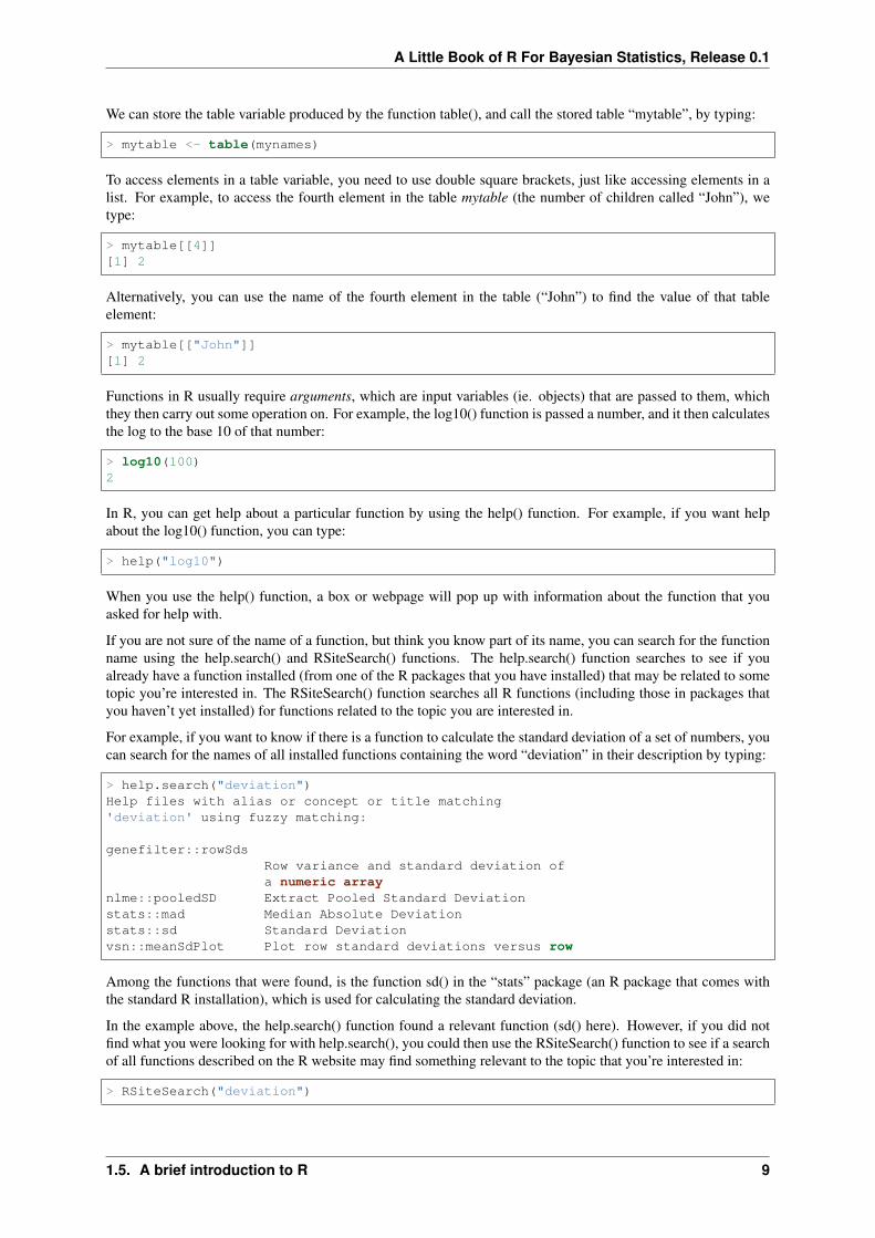
Functions in R usually require arguments, which are input variables (ie. objects) that are passed to them, whichthey then carry out some operation on. For example, the log10() function is passed a number, and it then calculatesthe log to the base 10 of that number:

> log10(100)2

In R, you can get help about a particular function by using the help() function. For example, if you want helpabout the log10() function, you can type:

> help("log10")

When you use the help() function, a box or webpage will pop up with information about the function that youasked for help with.

If you are not sure of the name of a function, but think you know part of its name, you can search for the functionname using the help.search() and RSiteSearch() functions. The help.search() function searches to see if youalready have a function installed (from one of the R packages that you have installed) that may be related to sometopic you’re interested in. The RSiteSearch() function searches all R functions (including those in packages thatyou haven’t yet installed) for functions related to the topic you are interested in.

For example, if you want to know if there is a function to calculate the standard deviation of a set of numbers, youcan search for the names of all installed functions containing the word “deviation” in their description by typing:

> help.search("deviation")Help files with alias or concept or title matching'deviation' using fuzzy matching:

genefilter::rowSdsRow variance and standard deviation ofa numeric array

nlme::pooledSD Extract Pooled Standard Deviationstats::mad Median Absolute Deviationstats::sd Standard Deviationvsn::meanSdPlot Plot row standard deviations versus row

Among the functions that were found, is the function sd() in the “stats” package (an R package that comes withthe standard R installation), which is used for calculating the standard deviation.

In the example above, the help.search() function found a relevant function (sd() here). However, if you did notfind what you were looking for with help.search(), you could then use the RSiteSearch() function to see if a searchof all functions described on the R website may find something relevant to the topic that you’re interested in:

> RSiteSearch("deviation")

1.5. A brief introduction to R 9


The results of the RSiteSearch() function will be hits to descriptions of R functions, as well as to R mailing listdiscussions of those functions.

We can perform computations with R using objects such as scalars and vectors. For example, to calculate theaverage of the values in the vector myvector (ie. the average of 8, 6, 9, 10 and 5), we can use the mean() function:

> mean(myvector)[1] 7.6

We have been using built-in R functions such as mean(), length(), print(), plot(), etc. We can also create our ownfunctions in R to do calculations that you want to carry out very often on different input data sets. For example,we can create a function to calculate the value of 20 plus square of some input number:

> myfunction <- function(x) { return(20 + (x*x)) }

This function will calculate the square of a number (x), and then add 20 to that value. The return() statementreturns the calculated value. Once you have typed in this function, the function is then available for use. Forexample, we can use the function for different input numbers (eg. 10, 25):

> myfunction(10)[1] 120> myfunction(25)[1] 645

To quit R, type:

> q()

1.6 Links and Further Reading

Some links are included here for further reading.

For a more in-depth introduction to R, a good online tutorial is available on the “Kickstarting R” website, cran.r-project.org/doc/contrib/Lemon-kickstart.

There is another nice (slightly more in-depth) tutorial to R available on the “Introduction to R” website, cran.r-project.org/doc/manuals/R-intro.html.

1.7 Acknowledgements

For very helpful comments and suggestions for improvements on the installation instructions, thank you verymuch to Friedrich Leisch and Phil Spector.

1.8 Contact

I will be very grateful if you will send me (Avril Coghlan) corrections or suggestions for improvements to myemail address [email protected]

1.9 License

The content in this book is licensed under a Creative Commons Attribution 3.0 License.


http://cran.r-project.org/doc/contrib/Lemon-kickstart/


http://cran.r-project.org/doc/manuals/R-intro.html




http://creativecommons.org/licenses/by/3.0/

CHAPTER 2

Using R for Bayesian Statistics

2.1 Bayesian Statistics

This booklet tells you how to use the R statistical software to carry out some simple analyses using Bayesianstatistics.

This booklet assumes that the reader has some basic knowledge of Bayesian statistics, and the principal focus ofthe booklet is not to explain Bayesian statistics, but rather to explain how to carry out these analyses using R.

If you are new to Bayesian statistics, and want to learn more about any of the concepts presented here, I wouldhighly recommend the Open University book “Bayesian Statistics” (product code M249/04), which you might beable to get from from the University Book Search.

There is a pdf version of this booklet available at https://media.readthedocs.org/pdf/a-little-book-of-r-for-bayesian-statistics/latest/a-little-book-of-r-for-bayesian-statistics.pdf.

If you like this booklet, you may also like to check out my booklets on using R for biomedicalstatistics, http://a-little-book-of-r-for-biomedical-statistics.readthedocs.org/, using R for time series analy-sis, http://a-little-book-of-r-for-time-series.readthedocs.org/, and using R for multivariate analysis, http://little-book-of-r-for-multivariate-analysis.readthedocs.org/.

2.2 Using Bayesian Analysis to Estimate a Proportion

Bayesian analysis can be useful for estimating a proportion, when you have some rough idea of what the value ofthe proportion is, but have relatively little data.

2.2.1 Specifying a Prior for a Proportion

An appropriate prior to use for a proportion is a Beta prior.

For example, if you want to estimate the proportion of people like chocolate, you might have a rough idea that themost likely value is around 0.85, but that the proportion is unlikely to be smaller than 0.60 or bigger than 0.95.

You can find the best Beta prior to use in this case by specifying that the median (50% percentile) of the prior is0.85, that the 99.999% percentile is 0.95, and that the 0.001% percentile is 0.60:

11

http://www.universitybooksearch.co.uk/



http://a-little-book-of-r-for-biomedical-statistics.readthedocs.org/

http://a-little-book-of-r-for-time-series.readthedocs.org/




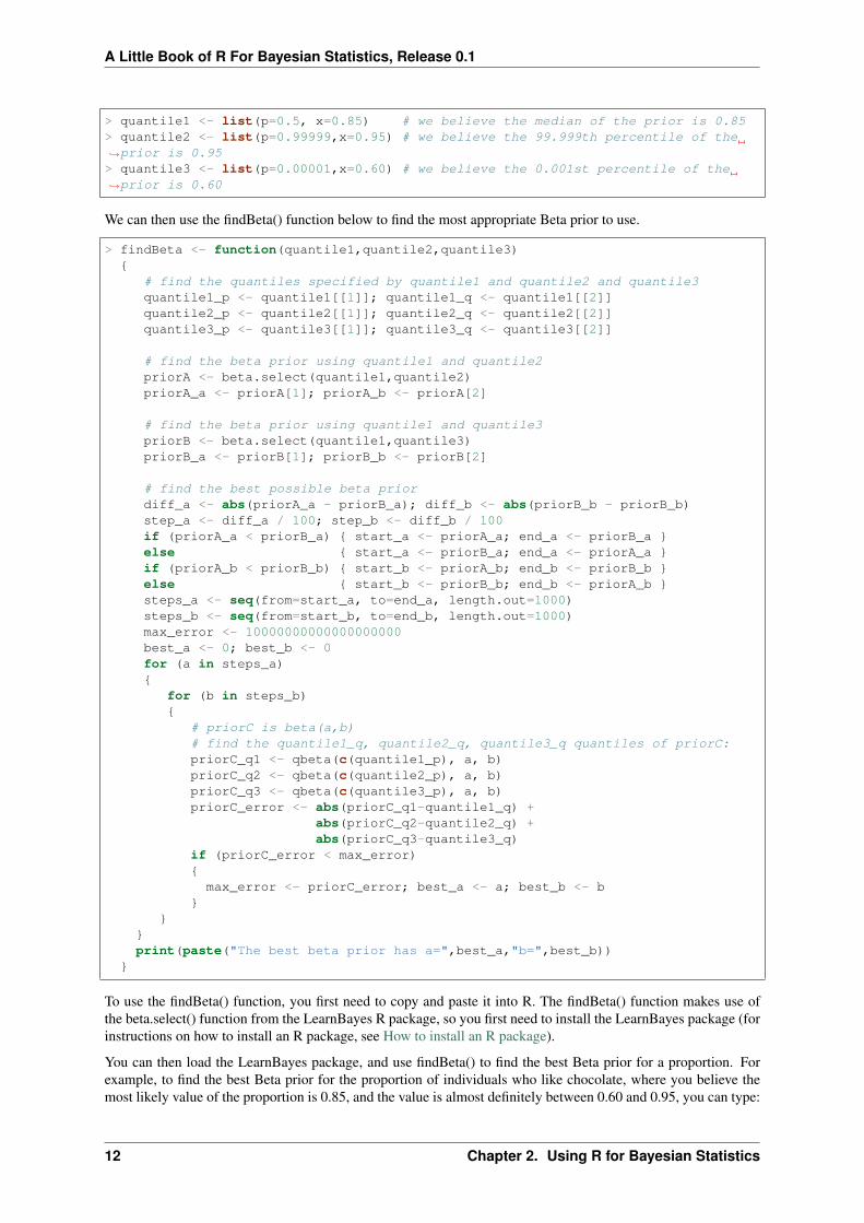
> quantile1 <- list(p=0.5, x=0.85) # we believe the median of the prior is 0.85> quantile2 <- list(p=0.99999,x=0.95) # we believe the 99.999th percentile of the→˓prior is 0.95> quantile3 <- list(p=0.00001,x=0.60) # we believe the 0.001st percentile of the→˓prior is 0.60

We can then use the findBeta() function below to find the most appropriate Beta prior to use.

> findBeta <- function(quantile1,quantile2,quantile3){

# find the quantiles specified by quantile1 and quantile2 and quantile3quantile1_p <- quantile1[[1]]; quantile1_q <- quantile1[[2]]quantile2_p <- quantile2[[1]]; quantile2_q <- quantile2[[2]]quantile3_p <- quantile3[[1]]; quantile3_q <- quantile3[[2]]

# find the beta prior using quantile1 and quantile2priorA <- beta.select(quantile1,quantile2)priorA_a <- priorA[1]; priorA_b <- priorA[2]

# find the beta prior using quantile1 and quantile3priorB <- beta.select(quantile1,quantile3)priorB_a <- priorB[1]; priorB_b <- priorB[2]

# find the best possible beta priordiff_a <- abs(priorA_a - priorB_a); diff_b <- abs(priorB_b - priorB_b)step_a <- diff_a / 100; step_b <- diff_b / 100if (priorA_a < priorB_a) { start_a <- priorA_a; end_a <- priorB_a }else { start_a <- priorB_a; end_a <- priorA_a }if (priorA_b < priorB_b) { start_b <- priorA_b; end_b <- priorB_b }else { start_b <- priorB_b; end_b <- priorA_b }steps_a <- seq(from=start_a, to=end_a, length.out=1000)steps_b <- seq(from=start_b, to=end_b, length.out=1000)max_error <- 10000000000000000000best_a <- 0; best_b <- 0for (a in steps_a){

for (b in steps_b){

# priorC is beta(a,b)# find the quantile1_q, quantile2_q, quantile3_q quantiles of priorC:priorC_q1 <- qbeta(c(quantile1_p), a, b)priorC_q2 <- qbeta(c(quantile2_p), a, b)priorC_q3 <- qbeta(c(quantile3_p), a, b)priorC_error <- abs(priorC_q1-quantile1_q) +

abs(priorC_q2-quantile2_q) +abs(priorC_q3-quantile3_q)

if (priorC_error < max_error){max_error <- priorC_error; best_a <- a; best_b <- b

}}

}print(paste("The best beta prior has a=",best_a,"b=",best_b))

}

To use the findBeta() function, you first need to copy and paste it into R. The findBeta() function makes use ofthe beta.select() function from the LearnBayes R package, so you first need to install the LearnBayes package (forinstructions on how to install an R package, see How to install an R package).

You can then load the LearnBayes package, and use findBeta() to find the best Beta prior for a proportion. Forexample, to find the best Beta prior for the proportion of individuals who like chocolate, where you believe themost likely value of the proportion is 0.85, and the value is almost definitely between 0.60 and 0.95, you can type:

12 Chapter 2. Using R for Bayesian Statistics

./installr.html#how-to-install-an-r-package


> library("LearnBayes")> findBeta(quantile1,quantile2,quantile3)

[1] "The best beta prior has a= 52.22 b= 9.52105105105105"

This tells us that the most appropriate prior to use for the proportion of individuals who like chocolate is a Betaprior with a=52.22 and b=9.52, that is, a Beta(52.22, 9.52) prior.

We can plot the prior density by using the “curve” function:

> curve(dbeta(x,52.22,9.52105105105105)) # plot the prior

Note that in the command above we use the “dbeta()” function to specify that the density of aBeta(52.22,9.52105105105105) distribution.

We can see from the picture of the density for a Beta(52.22,9.52105105105105) distribution that it represents ourprior beliefs about the proportion of people who like chocolate fairly well, as the peak of the distribution is atabout 0.85, and the density lies almost entirely between about 0.68 and 0.97.

2.2.2 Calculating the Likelihood Function for a Proportion

Say you want to estimate a proportion, and you have a small data set that you can use for this purpose. Forexample, if you want to estimate the proportion of people who like chocolate, you may have carried out a surveyof 50 people, and found that 45 say that they like chocolate.

This small data set can be used to calculate the conditional p.m.f. (probability mass function) of the proportiongiven the observed data. This is called the likelihood function. It represents how likely the possible values of theproportion are, given the observed data.

If you want to estimate a proportion, and have a small data set, you can calculate the likelihood function for theproportion using the function calcLikelihoodForProportion() below:

> calcLikelihoodForProportion <- function(successes, total){

curve(dbinom(successes,total,x)) # plot the likelihood}

The function calcLikelihoodForProportion() takes two input arguments: the number of successes observed in thesample (eg. the number of people who like chocolate in the sample), and the total sample size.

You can see that the likelihood function is being calculated using the Binomial distribution (using the R “dbinom()”function). That is, the likelihood function is the probability mass function of a B(total,successes) distribution, that

2.2. Using Bayesian Analysis to Estimate a Proportion 13


is, of a Binomial distribution where the we observe “successes” successes out of a sample of “total” observationsin total.

For example, if we did a survey of 50 people, and found that 45 say they like chocolate, then our total sample sizeis 50 and we have 45 “successes”. We can calculate the likelihood function for the proportion of people who likechocolate by typing:

> calcLikelihoodForProportion(45, 50)

You can see that the peak of the likelihood distribution is at 0.9, which is equal to the sample mean (45/50 = 0.9).In other words, the most likely value of the proportion, given the observed data, is 0.9.

2.2.3 Calculating the Posterior Distribution for a Proportion

Say you are trying to estimate a proportion, and have a prior distribution representing your beliefs about thevalue of that proportion. If you have collected some data, you can also calculate the likelihood function for theproportion given the data.

However, after observing the data, you may wish to update the prior distribution for the proportion, taking the datainto consideration. That is, you may wish to calculate the conditional distribution of the proportion given the dataand the prior. This is is called the posterior distribution for the proportion.

The posterior distribution ssummarises what is known about the proportion after the data has been observed, andcombines the information from the prior and the data.

In our example of estimating the proportion of people who like chocolate, we have a Beta(52.22,9.52) prior distri-bution (see above), and have some data from a survey in which we found that 45 out of 50 people like chocolate.We can calculate the posterior distribution for the proportion given the prior and data using the calcPosteriorFor-Proportion() function below (which I adapted from “triplot” in the LearnBayes package):

> calcPosteriorForProportion <- function(successes, total, a, b){

# Adapted from triplot() in the LearnBayes package# Plot the prior, likelihood and posterior:likelihood_a = successes + 1; likelihood_b = total - successes + 1posterior_a = a + successes; posterior_b = b + total - successestheta = seq(0.005, 0.995, length = 500)prior = dbeta(theta, a, b)likelihood = dbeta(theta, likelihood_a, likelihood_b)posterior = dbeta(theta, posterior_a, posterior_b)m = max(c(prior, likelihood, posterior))plot(theta, posterior, type = "l", ylab = "Density", lty = 2, lwd = 3,

main = paste("beta(", a, ",", b, ") prior, B(", total, ",", successes,→˓") data,",



"beta(", posterior_a, ",", posterior_b, ") posterior"), ylim = c(0, m),→˓col = "red")

lines(theta, likelihood, lty = 1, lwd = 3, col = "blue")lines(theta, prior, lty = 3, lwd = 3, col = "green")legend(x=0.8,y=m, c("Prior", "Likelihood", "Posterior"), lty = c(3, 1, 2),

lwd = c(3, 3, 3), col = c("green", "blue", "red"))# Print out summary statistics for the prior, likelihood and posterior:calcBetaMode <- function(aa, bb) { BetaMode <- (aa - 1)/(aa + bb - 2);

→˓return(BetaMode); }calcBetaMean <- function(aa, bb) { BetaMean <- (aa)/(aa + bb);

→˓return(BetaMean); }calcBetaSd <- function(aa, bb) { BetaSd <- sqrt((aa * bb)/(((aa + bb)^2) *

→˓(aa + bb + 1))); return(BetaSd); }prior_mode <- calcBetaMode(a, b)likelihood_mode <- calcBetaMode(likelihood_a, likelihood_b)posterior_mode <- calcBetaMode(posterior_a, posterior_b)prior_mean <- calcBetaMean(a, b)likelihood_mean <- calcBetaMean(likelihood_a, likelihood_b)posterior_mean <- calcBetaMean(posterior_a, posterior_b)prior_sd <- calcBetaSd(a, b)likelihood_sd <- calcBetaSd(likelihood_a, likelihood_b)posterior_sd <- calcBetaSd(posterior_a, posterior_b)print(paste("mode for prior=",prior_mode,", for likelihood=",likelihood_mode,

→˓", for posterior=",posterior_mode))print(paste("mean for prior=",prior_mean,", for likelihood=",likelihood_mean,

→˓", for posterior=",posterior_mean))print(paste("sd for prior=",prior_sd,", for likelihood=",likelihood_sd,", for

→˓posterior=",posterior_sd))}

To use the “calcPosteriorForProportion()” function, you will first need to copy and paste it into R. It takes fourarguments: the number of successes and total sample size in your data set, and the a and b values for your Betaprior.

For example, to estimate the proportion of people who like chocolate, you had a Beta(52.22,9.52) prior and hadobserved in a survey that 45 out of 50 people like chocolate. Therefore, the number of successes is 45, the samplesize is 50, and a and b for the prior are 52.22 and 9.52 respectively. Therefore, we can calculate the posterior forthe proportion of people who like chocolate, given the data and prior, by typing:

> calcPosteriorForProportion(45, 50, 52.22, 9.52)[1] "mode for prior= 0.857381988617342 , for likelihood= 0.9 , for posterior= 0.

→˓876799708401677"[1] "mean for prior= 0.845804988662132 , for likelihood= 0.884615384615385 , for

→˓posterior= 0.870055485949526"[1] "sd for prior= 0.0455929848904483 , for likelihood= 0.0438847130123102 , for

→˓posterior= 0.0316674748482802"

2.2. Using Bayesian Analysis to Estimate a Proportion 15


Since the prior and posterior are distributions, the area under their densities is 1. The likelihood has been scaledso that the area underneath it is also 1, so that it is easy to compare the likelihood with the prior and posterior.

Therefore, the prior and likelihood curves should look the same shape as those plotted before (see above), but they-axis scale is different for the likelihood scale compared to the plot made using calcLikelihoodForProportion()above.

Note that the peak of the posterior always lies somewhere between the peaks of the prior and the likelihood,because it combines information from the prior and the likelihood (which is based on the data).

In our example of estimating the proportion of people who like chocolate, the peak of the posterior is roughlyhalf-way between the peaks of the likelihood and prior, indicating that the prior and the data contribute roughlyequally to the posterior.

2.3 Links and Further Reading

Here are some links for further reading.

For a more in-depth introduction to R, a good online tutorial is available on the “Kickstarting R” website, cran.r-project.org/doc/contrib/Lemon-kickstart.

There is another nice (slightly more in-depth) tutorial to R available on the “Introduction to R” website, cran.r-project.org/doc/manuals/R-intro.html.

To learn about Bayesian Statistics, I would highly recommend the book “Bayesian Statistics” (product codeM249/04) by the Open University, available from the Open University Shop.

There is a book available in the “Use R!” series on using R for multivariate analyses, Bayesian Computation withR by Jim Albert.






http://www.ouw.co.uk/store/

http://www.springer.com/statistics/statistical+theory+and+methods/book/978-0-387-92297-3

http://www.springer.com/statistics/statistical+theory+and+methods/book/978-0-387-92297-3


2.4 Acknowledgements

Many of the examples in this booklet are inspired by examples in the excellent Open University book, “BayesianStatistics” (product code M249/04), available from the Open University Shop.

2.5 Contact

I will be grateful if you will send me (Avril Coghlan) corrections or suggestions for improvements to my emailaddress [email protected]

2.6 License


2.4. Acknowledgements 17

http://www.ouw.co.uk/store/




CHAPTER 3

Acknowledgements

Thank you to Noel O’Boyle for helping in using Sphinx, http://sphinx.pocoo.org, to create this document, andgithub, https://github.com/, to store different versions of the document as I was writing it, and readthedocs, http://readthedocs.org/, to build and distribute this document.

19

http://sphinx.pocoo.org

https://github.com/

http://readthedocs.org/

http://readthedocs.org/


20 Chapter 3. Acknowledgements

CHAPTER 4

Contact

I will be very grateful if you will send me (Avril Coghlan) corrections or suggestions for improvements to myemail address [email protected]

21




22 Chapter 4. Contact

CHAPTER 5

License


23


a little book of r for bayesian statistics

Documents