a laser-guided, autonomous automated … · few (hollier, 1987). overall, the changing marketplace...
TRANSCRIPT

A LASER-GUIDED,
AUTONOMOUS AUTOMATED GUIDED VEHICLE
by
Jeff E. Fithian
Thesis submitted to the Faculty of the
Virginia Polytechnic Institute and State University
in partial fulfilment of the requirements for the degree of
MASTER OF SCIENCE
in
INDUSTRIAL AND SYSTEMS ENGINEERING
Approved:
Dr. Michael P. Deisenroth
Dr. Roderick J. Reasor
June, 1993
Blacksburg, Virginia

Li) ~6£~
V'6~5 I Cj'1.3 rCj44
elL.

ACKNOWLEDGMENTS
The author would like to express his appreciation to the members of his committee,
Drs. Michael P. Deisenroth, Yvan J. Beliveau, and Roderick J. Reasor for their assistance
in conducting this research and preparing this thesis. I would especially like to thank Dr.
Beliveau for the use of the only existing positioning system owned by his company, Spatial
Positioning Systems, Inc. and for his ideas in developing the navigation algorithm for the
system. I would also like to thank Eric Lundberg of SPSi for arranging to the use of the
equipment and Andrew Dornbush of SPSi for technical support with the system, without
whose help the research would have taken much longer and caused many more headaches.
I would like to thank Mr. Rod Hall of the Corporate Research Center at Virginia Tech for
the use of his building to perform my experiment. Thanks also to Dave Nicks for his
critical proof-reading and his ability to easily solve problems which tended to keep me
awake at night, and for the use of his printer to chum out hundreds of pages of rough draft.
Finally, but by no means lastly, I would like to thank my parents whose love and support
has given me courage in this, and in all of my pursuits, to always do my best.
ii

TABLE OF CONTENTS
ACKNOWLEDGEMENTS .................................................... i i
LIST OF FIGURES ........................................................... vi
CHAPTER 1 INTRODUCTION ............................................................. 1
History and Background of AGVs 0 ••••••••• ; ••• 0 •••••••••••••••••••••••••••••••••••••• 1 History .................................................... o ••••••••••• 0 ••••••••••• 1 Necessity for AGVs ............................................................. 2 Advantages and Disadvantages of AGVs ..................................... 4 Applications of AGV s .......... o •••••••••••••••••••••••••••••••••••••••••••••••• 8
AGV System Components ............................................................... 8 Physical COmponents ........................................................... 8 Control Systems ................................................•................ 9
AGV Navigation Methods ......................................... o ••••••••••••••••••••• 10 Types of Navigation ............................................................. 11 Advantages of Autonomous Navigation ...................................... 13
Research Topic ............................................................................ 15 Problem Statement ............................................................... 15 Research Objectives .......................................................... 0 •• 15 Relevance of Study ..............•............................................... 15
CHAPTER 2 LITERA. TURE REVIEW ...................................................... 1 7
Introduction ....................................•........................................... 17 Dead-Reckoning-Based Systems ........ 0.0 •••••••• 0 •••••••• 0 •••••••••••••••• 0 •••• 0 •••• 17 Beacon-Based Systems .................................................................. 19 Vision- and Mapping- Based Systems ........................................... 0 ••••• 22 Conclusions ..............................................................•................ 23
CHAPTER 3 METHODOLOG Y .............................................................. 1S
Introduction ............................................. 0 •••••••••••••••••• 00 •••••••••••••• 25 Path Generation Software .........................................•...................... 25 Hardware Installation and Debugging .................................................. 28
Laser-Based Positioning System ............................................... 28 Hardware and Software for Trajectory and Path Calculations .............. 30 The Autonomous Guided Vehicle .............................................. 30
System Testing and Analysis of Results ... 0 •• o. 0 •••••••••••••••••••••••••••••••••••••• 33
CHAPTER 4 PATH GENERATION ......................................................... 36
Introduction ........................ 0 •••••••••••••••••••••••••••••••• 0 •••••••••••••••••••••• 36 Methodology ............................•.......•......................................... 36
Drawing Interchange File Format. ................................... 0 ••••••••• 36 Arc Blending ..................................................................... 40 Path Segment Generation ....................................................... 44
Path Generation Software ................................................................ 46 Main Menu Options .............................................................. 47
iii
Change Parameters Menu ....................................................... 47 Conclusions ............................................................................... 50
CHAPTER 5 NAVIGATION .............................................................. ..•. 51
Introduction ................................................................................ 51 Methodology .............................................................................. 51 Navigation Software ...................................................................... 54
Main Menu Options .............................................................. 54 Change Parameters Menu ....................................................... 57
Conclusions ............................................................................... 60
CHAPTER' RESULTS AND DISCUSSION .............................................. , 1
System Set-Up and Calibration ......................................................... 61 Test Results ................................................................................ 63
Test 1: Straight Line Path ....................................................... 63 Test 2: Three Segment Path ..................................................... 75 Test 3: Two Segment Path ......................................... 0 •••• 0 ••• 0 ••• 84
Further DiscussionlProblems Encountered 0 ••••••••••••••••••••••••••••••••••••••••••• 91 Low Range of Positioning System .. 0 •••• 0 •••••••••• 0 ••••••• 0 ••••••••••• 0 ••••• 92 Low Reliability Outside Region of Higher Accuracy ... 0 •••• 0 ••••••••••••••• 92 Blocking of Lasers From Receiver .......... 0.0 ••• 0 •• 0 •••••••••••••••••••••••• 93 Extraneous Light Interference. 0 0 ••••••••••••••••••••••••••••••••••• 0 ••••••••••• 93 Overall System Reliability 0 •• 0 •••••••••••••••••••••••••••••••••••••••••••••••••• 93 DXF File Problem ............................................................... 93 Delay of Positioning System ................................................... 94
CHAPTER 7 CONCLUSIONS .••....••.••••.•••••.•.•••••••..•.•.••.•.••••••.•••...••.•••••. 95
Future Areas of Research ................................................................ 98 Heading Detennination .......................................................... 98 Minimum Update Distance ...................................................... 98 Error Recovery ................................................................... 99 Regulate Vehicle Velocity ........................................ 0 ••••• 0 0 ••••••• 99 Filtering of Invalid Data ......................................................... 100 Next Generation System ................................. 00. 0 ••••••••••••••• 0.' .100 Outdoor Navigation .............................................................. 100 Path Generation and Navigation Software .........................•........... 100
REFERENCES .•..•.•.•.........•......•.......••..•.•..•.•..••.....•..•••...•. 101
APPENDIX A Sample DXF Data. File ...••••.•...............•...•••...•...••..•••••.•...•.•. 104
APPENDIX B Path Generation Software Program Listing ..•..•.•...•••••...•••.....•.••.. 108
APPENDIX C Navigation Software Program Listing ........•...•••••..•••.•••..••••••.•••• 121
APPENDIX D Parameter Listing for Testing .••.••••....••.•••••••••....•.......•....•..•.•. 15'
iv

VITA .••••...•..•.•......••••••...•..............••••••••.••....••••••••...•••.• 162
ABSTRACT
v

Figure 3.1a
Figure 3.1h
Figure 3.1c
Figure 3.2
Figure 3.3
Figure 3.4
Figure 3.5
Figure 3.6
Figure 4.1
Figure 4.2
Figure 4.3
Figure 4.4
Figure 4.5
Figure 4.6
Figure 4.7
Figure 4.8
Figure 5.1
Figure 5.2
Figure '5.3
Figure 5.4
Figure 5.5
Figure 6.1
Figure 6.2
Figure 6.3
Figure 6.4
Figure 6.5
Figure 6.6
Figure 6.7
Figure 6.8
Figure 6.9
Figure 6.10
Figure 6.11
LIST OF FIGURES
Discontinuous Path Definition ............................................. 26
Invalid Turnaround in Path Definition •................................... 26
Valid Path Definition ........................................................ 27
Path Before and After Adding Arc Transitions .......................... 27
Receiver Mounted on AGV ................................................ 29
Reference Point on Vehicle ................................................. 31
Hardware and Software Diagram .......................................... 32
Region of Expected High Accuracy ....................................... 34
Path diagram in CANVAS graphi~ software ........................... 37
Saving the drawing as a ".dxf" file in CANVAS ........................ 38
Linear Path Segment Vector within Path Coordinate System .......... 41
Untransformed Segment Vectol'S in the
Vector Coordinate System .................................................. 42
l...<:lcation of Arc .............................................................. 43
Path Before and After Arc Blending ...................................... 45
Path Generation Software Main Menu Screen ........................... 46
Change Parameters Menu in Path Generation Software .........•...... 48
Path Points: ..............................•..................•....•............ 52
Angle Conventions for Navigation .......................................... 52
Determination of AGV Position Along Vector Connecting Two
Path Points .................................................................... 54
Main Menu Screen for Navigation Software ............................. 55
Change Parameters Menu for Navigation Software ...•................. 58
Layout of System During Testing ......................................... 62
Path #1 ........................................................................ 64
Results of Test la .... ,. .... ,. ......................... ,. ...................... . 65
Results of Test lb ........................................................... 66
Results of Test Ie ............................................................. 68
Results of Tests Ie and If After Removing Invalid Data ............... 69
Results of Test 1h ............................................................. 71
Results of Test 1m .......................•.•................................ 72
Results of Test Ip ........................................................... 74
Path #2 ........................................................................ 75
Results of Test 2a •........•.•.•.•.•.•.•••••..•..•.•••••••••••..••••••..••..• 77
vi

Figure 6.12
Figure 6.13
Figure 6.14
Figure 6.15
Figure 6.16
Figure 6.17
Figure 6.18
Figure 6.19
Figure 6.20
Figure 6.21
Results of Test 2d ........................................................... 78
Results of Test 2h ........................................................... 80
Results of Test 21 ............................................................ 81
Results of Test 2m .......................................................... 82
Results of Test 20 ................................................•.......... 83
Path #3 .••.•••••••••.•..•.......•..••••......•••••••••••.................•..... 84
Results of Test 3c ••••••••••••••••••.•...••••••••••••••••••••••••••••••••.••• 86
Results of Test 3g ........................................................... 88
Results of Test 31 ............................................................ 89
Results of Test 3m .......................................................... 90
vii

CHAPTER 1
INTRODUCTION
HISTORY AND BACKGROUND OF AGVS
History
An Automatic Guided Vehicle (AGV) can be defined as a material handling or
conveying vehicle whose purpose is to navigate around some workspace without the use of
a human driver. According to the most popular definitions, all vehicles which require a
human operator or ride on rails are not considered AGVs (Hollier, 1987).
The vehicle is usually controlled by one or more computers, depending on the
complexity and autonomy of the vehicle. In the case of a conventional, wire- or tape
guided vehicle this computer will give instructions to the AGV telling it where to go and,
usually, how to get there. In the case of an autonomous vehicle, the computer(s) will need
to perform much more complex operations to determine position, examine the
surroundings, plan the next move, etc. The computer can also give special instructions to
the AGV such as a command to move to the charging area or to stop on the path for traffic
reasons. The vehicle usually follows a defined path, whether it is a wire in the floor or a
path mapped into the computer's memory.
In the past few years AGVs have become increasingly popular as a replacement for
traditional fork-lift type material handling applications. This popularity can be
demonstrated by the numerous international conferences on AGVs which have taken place
since 1981. In addition, the vast amount of AGV literature available today also is a credit
to the rising popularity and importance of AGVs. The work on AGVs in academia is
further supported by the ever increasing number of AGVs implemented today in many
1

different industries, including automotive, electronic, assembly, and clean-room
environments.
The first vehicle to actually be called an Automatic Guided Vehicle and which fits
the definition above was developed in the 1950's by Barrett Electronics in the USA. The
first installation of an AGV system followed at Mercury Motor Freight in Columbia, South
Carolina in 1954. This system used vacuum tube technology for its controller and used an
inductive wire for navigation (Hollier, 1986).
Although AGVs were originally developed in the USA, after the 1960's, AGVs
caught on much faster in Europe than in the USA. Some of the reasons for this were
outlined by Hammond (AGVs at Work, 1986):
• The European work force does not view automation as a threat to job security.
• The advent of standardized European pallet dimensions.
• The longer-term payback periods which are acceptable in European industry.
• The necessity of automation due to stricter safety and work environment
regulations.
• The existence of a more stable work force which is necessary to maintain highly
trained personnel for the operation and maintenance of automation equipment.
Thus, the USA has fallen behind in many areas of AGV design and
implementation. However, due to reasons outlined in the next section, the USA is again
committing to AGVs.
Necessity for AGVs
As industry has become more competitive and world-markets have expanded,
American industry has re-evaluated its commitment to automation. Some of the major
reasons for this are Hammond (AGVs at Work, 1986):
2

• Foreign competition has become more intense.
• Many AGV vehicles and systems are now being developed and marketed by
European companies and sold to firms in the USA
• The recessions of the late 1970's and early 1980's, and of the early 1990's has
damaged the US automobile industry to the point where they must look for
more efficient ways to produce cars.
• The unions' acceptance of new automation technology as a path to higher job
security in lieu of pay raises.
• Advances in micro-processors which permit them to be mounted on-board
allowing the vehicles to interface with the "modernization" taking place in US
industries.
In addition, material handling costs make up a high proportion of overall operation
costs. Although an AGV system may appear to incur higher costs than a manual system at
first, an AGV system exhibits intangible cost advantages such as increased material
handling control and flexibility, reduced product damage, and space reduction to name a
few (Hollier, 1987).
Overall, the changing marketplace has placed the following demands upon
manufacturing firms, and AGVs propose a viable solution to achieving these goals
(Horrocks, 1989):
• Reduce costs
• Raise productivity
• Achieve faster response times
• Consistently deliver on-time
• Improve quality to 100%
• Increase flexibility
3

The next section will detail some of the advantages of AGVs which demonstrate
how they can help attain these goals.
Advantages and Disadvantages of AGVs
Because industry is turning to the use of AGVs as an important method of reaching
competitive business goals, it is important to point out some of the advantages and
disadvantages of AGVs.
Advantages
Hammond (AGVs at Work, 1986) and Yates (1988) list some advantages which
AGV systems offer. They are:
Labor Savings - By increasing the material handling capacity of a facility
without increasing manpower, AGVs effectively reduce the labor effort
necessary per job.
Increased Quality and Productivity - AGVs have the ability to be integrated
into an assembly line environment much better than a typical conveyor belt due
to their ability to stop and go during material handling operations. This allows
the workpiece to be stationary while the operator works and reduces operator
fatigue, thus reducing mistakes and improving quality.
Job Enrichment and Worker Satisfaction - An AGV can position a
workpiece much better than a conveyor belt by rotating or turning the piece for
better operator accessibility. Furthermore, the worker can work at his/her own
pace, instead of that of a synchronous conveyor belt. Another advantage is the
spirit of team work which can be created by parallel workstations made possible
by AGVs.
4

Improved Control - AGVs can keep track of what load they are carrying,
therefore providing real-time control of inventory. In addition, AGVs do not
take breaks while delivering goods or get interrupted by other workers. In
short, AGVs can be very disciplined when moving material.
Reduced Space Requirements - Because AGVs track so accurately, aisles
can often be narrower than with conventional fork trucks. In addition, the
better control of inventory can result in reduced work-in-progress, meaning less
inventory on the floor and less floor space requirements.
Reduced Product Damage - Because a work piece may remain with the
vehicle at all times, the possibilities of damage while being moved from a fork
truck to a conveyor are reduced. Also, AGVs, by nature, handle material in a
more controlled manner which reduces the chances of product damage during
handling.
Housekeeping Improvements - AGVs do not create the same types of wastes
and contaminants that traditional conveyor-type systems create.
Ease of Removal and Installation - With the exception of the guidewire
removal (if applicable), the AGV system can be easily relocated and re-installed.
One must, however, consider the programming costs associated with relocating
an AGV system.
Easy Integration with Automation - Due to its computer-controlled nature,
an AGV is easier to integrate with a factory automation system than a traditional
material handling system.
Adaptability and Flexibility - Modifying or expanding an AGV system is
relatively easy compared with a traditional material handling system such as a
conveyor. It is important, however, to make sure that the original system was
designed with flexibility and growth in mind.
5

Consistent Material Flow - Due to their ability to vary speed and be used
only on an "as needed" basis, AGVs can take potentially uneven material flow
and transform it to steady material flow without the problems of accumulation
one can encounter with a conveyor belt.
Hazardous Environments - In these days of increasing employee health
costs, using AGVs in extreme temperature or dangerous chemical conditions
can greatly reduce medical liabilities of a company. In addition, the reduced
noise of electrical-drive vehicles makes for a better work environment and less
chances of hearing-related medical problems.
Multi-Shift Working - The same AGV can work around the clock with breaks
only for recharging.
Improved Floor Access - Conveyors can block off areas of the floor,
whereas AGVs travel in such a manner which in no way obstructs the floor
area.
Disadvantaies
Although there are many advantages offered by AGVs, the reader must be aware of
some of the disadvantages and problems which may be associated with AGVs. Some of
these drawbacks result from inadequate planning and/or management of the system, and
can be avoided. Hammond (AGVs at Work, 1986) listed some of the major disadvantages
ofAGVs:
Expense - AGV systems may cost two to three times more than conventional
conveyor type systems, while saving only 10-15% on labor. However, some
small-scale AGV installations have experienced a payback period of only one
year. It is important to realize the value of the intangible advantages of AGVs
(quality, safety, product damage) than merely considering labor savings alone.
6

External Use - The reliability of AGVs in extreme cold, outdoor conditions
may not be as good as that of a conventional fork truck.
Sensitivity to Floor Surface - For most guidance methods, the reliability of
the AGV is also heavily reliant on the condition of the floor. This becomes
especially important when using an autonomous navigation technique such as
dead-reckoning.
Guide-Path Bed Stability - A system using an embedded wire may be
damaged by floor-bed shifting of concrete or asphalt.
Problems with Metal Floors - Due to the reliance on a magnetically charged
inductive wire, an embedded-wire AGV cannot run over metal floors. This is
also the case when crossing a metal area of the floor where the AGV must lose
track of the guide wire and navigate without wire guidance.
Management Support - One of the most important success factors of an AGV
system installation is upper-management support. This includes providing
adequate training and dedicating maintenance personnel to the system. Without
this support, the system is doomed to failure.
Worker Attitudes - In addition to management, workers must support the
system and not see it as a threat to their jobs. In some cases, systems have even
been sabotaged by unhappy workers.
Obstructions - When a human operator is driving a fork-truck, the driver can
avoid obstructions placed in the path of the truck. However, an AGV will
usually only be able to identify that something is in the path and come to a stop.
Installing an AGV system will require controlling all inventory and stocks and
making sure no objects get placed in the path of the AGV. This can also be an
advantage of the system in that is forces the company to practice good
housekeeping.
7

Inclined Surfaces - AGVs are usually limited to 4-6% inclines, although
inclines as high as 10% have been traversed by AGVs. However, even if this
is possible, its affect on the AGV (motor overheating, bearing stress) over the
long-term needs to be considered.
Maintenance - AGVs are much more complex than traditional material handling
systems and generally have higher maintenance costs.
Applications of AGV s
There are increasing opportunities for AGVs in many areas of industry today. In
addition to the conventional material handling functions in manufacturing, research is being
performed to examine the possibilities of mounting robot manipulators on AGVs which
will allow AGVs to function as a mobile workcenter (Piepel, 1989). However, at present,
AGVs are used in industry mainly to perform material movement and staging functions.
Some of the most popular areas of AGV applications are in the automotive, electronics,
postal, and food and tobacco industries (Hammond, Evolutionary AGVs: From Concept to
Reality, 1986, Miiller, 1987).
AGV SYSTEM COMPONENTS
An AGV system consists of three major components: the vehicle itself, the control
system, and the navigation system.
Physical Components
The physical components of an AGV system refer to the actual vehicle itself. Due
to the increasing complexity of vehicles on the market today, and the increasing variety of
applications, it is becoming more and more difficult to standardize vehicle design to cover
8

all applications. Therefore, it would be useless to describe a vehicle in terms of physical
size and shape. Rather, a vehicle can be described in terms of its major physical
components and the purpose or function of those comJXlnents. It is then up to the reader to
determine how these comJXlnents may be configured depending on the application in mind.
In general, an AGV will usually have a frame, a drive mechanism including
steering, a microcomputer for on-board control and system communication, a power
controller, and a battery on board (McEllin, 1987, Hammond, AGVs at Work, 1986). In
addition, modules can be attached to the AGV depending on the application. An example
of this would be a robot manipulator as mentioned above.
Control Systems
All AGVs which are used in an industrial setting must have some way of
communicating with the plant floor in order to know when and where to pick up loads and
to communicate status information back to the plant floor computer. Depending on the
level of intelligence built into the vehicle, the amount of information needed by the AGV
will differ. Some vehicles will be able to determine their own path to a particular
workstation, while others will be directed by a higher level computer exactly where to go.
The overall control of an AGV consists of two functions. The first function
concerns information about the materials being moved in terms of what is on the floor,
where it is, and how much is there. The second function concerns the physical aspect of
the materials in terms of what is needed, where it needs to be, and when it needs to be
there. An ideal control system will be able to address all of these needs, either at the plant
or AGV level (Hammond,AGVs at Work, 1986).
The two main methods of AGV system control are centralized and decentralized or
distributed (Hammond, AGVs at Work, 1986, Lindgren, 1987). A decentralized control
system works by having control sub-stations located around the AGV path, with each sub-
9

station responsible for its own inductive loop section in the system. A disadvantage of this
can be the complexity associated with many inductive loops for large systems. A large
computer acts as a central controller and speaks to each of these sub-stations, which in tum
send instructions and receive status information from the AGVs. The central computer
never communicates with individual AGVs in this type of control structure. The
advantages of this system is that the control is passed to as low a level as possible,
allowing each sub-station to act as a stand alone unit. The advantage to this is that if one
sub-station fails, the entire material handling system will not fail with it. This type of
control system also tends to be faster in terms of response time since all processing is done
at a lower level. The decentralized control system can also keep better track of AGV
positions since each vehicle reports directly to the sub-station.
In a central control scheme, a central material handling computer will communicate
directly to the AGVs (and other material handling equipment). In this method a central
processing unit will control all material handling devices in the area. The advantages of
centralized control are that it requires less equipment and personnel, is easy to back-up, and
it keeps all information centrally located in one location. Another advantage is that
compared with the inductive loops required for decentralized control, less floor cutting is
required and hence, installation and modification is cheaper and easier. A disadvantage,
however, can be the multitude of radio frequencies needed when using many AGVs.
AGV NAVIGATION METHODS
This research will concentrate on the navigation of an AGV using a laser-based
positioning system. Therefore, it is important to give a detailed background on navigation
methods for AGVs to the reader.
10
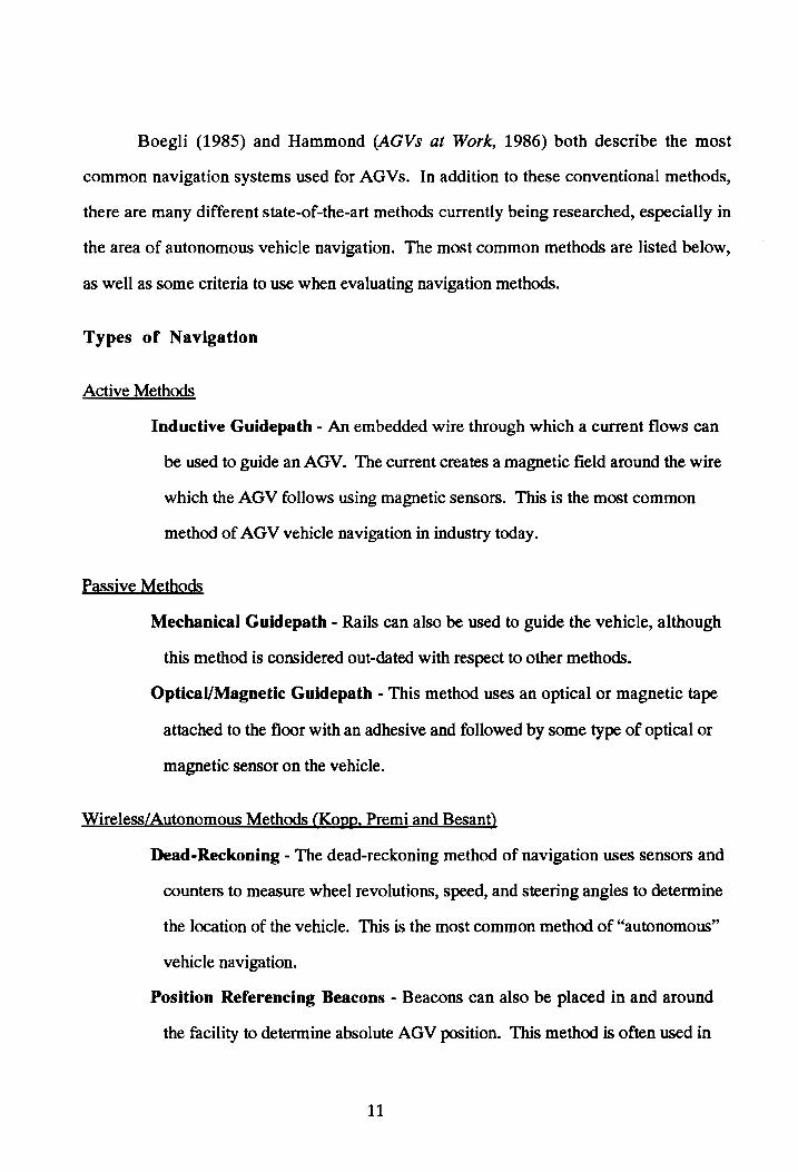
Boegli (1985) and Hammond (AGVs at Work, 1986) both describe the most
common navigation systems used for AGVs. In addition to these conventional methods,
there are many different state-of-the-art methods currently being researched, especially in
the area of autonomous vehicle navigation. The most common methods are listed below,
as well as some criteria to use when evaluating navigation methods.
Types of Navigation
Active Methods
Inductive Guidepath - An embedded wire through which a current flows can
be used to guide an AGV. The current creates a magnetic field around the wire
which the AGV follows using magnetic sensors. This is the most common
method of AGV vehicle navigation in industry today.
Passive Methods
Mechanical Guidepath - Rails can also be used to guide the vehicle, although
this method is considered out-dated with respect to other methods.
Optical/Magnetic Guidepath - This method uses an optical or magnetic tape
attached to the floor with an adhesive and followed by some type of optical or
magnetic sensor on the vehicle.
Wireless/Autonomous Methods (KoRP. Premi and Besant)
Dead-Reckoning - The dead-reckoning method of navigation uses sensors and
counters to measure wheel revolutions, speed, and steering angles to determine
the location of the vehicle. This is the most common method of "autonomous"
vehicle navigation.
Position Referencing Beacons - Beacons can also be placed in and around
the facility to determine absolute AGV position. This method is often used in
11

conjunction with dead-reckoning to provide absolute referencing to eliminate
accumulated error problems inherent to dead-reckoning systems.
Triangulation - Triangulation is a method which consists of receiving signals
(Radio frequency, light, laser) from transmitting beacons and determining the
position of the vehicle based on the received angle of two points. Some of the
drawbacks of this system are its cost, the difficulty in measuring a moving
object, and its range. The system used in this research, however, has a range
of up to 250 meters.
Inertial Navigation/Gyroscopic System - Gyroscopes can be used to
measure the translational and rotational acceleration of the vehicle to determine
its position. Since this method measures acceleration only, any deviation from
the path at constant velocity will not be detected.
Pattern Recognition/Machine Vision System - Using pattern recognition
or machine vision, the vehicle navigates by "recognizing" its surroundings and
respond according to some map programmed into the memory of the controlling
computer. This method is still very much in the research stage and will require
much more computer power than is currently available to be feasible for
industrial applications. A subset of this method involves placing cameras at
various points within the facility and having them locate the vehicles by taking
pictures of the factory floor. This method is cheaper and faster than true image
processing.
Infrared - Using this method, the vehicle can "home-in" on infrared beacons
strategically located in the area. The disadvantage is that the vehicle must be
able to maintain a line of sight to the beacons at all times.
Radio - Radio waves can be used to locate the position of a vehicle at a range of
100 meters up to thousands of kilometers. However, the accuracy of this
12
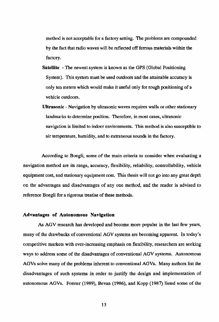
method is not acceptable for a factory setting. The problems are compounded
by the fact that radio waves will be reflected off ferrous materials within the
factory.
Satellite - The newest system is known as the GPS (Global Positioning
System). This system must be used outdoors and the attainable accuracy is
only ten meters which would make it useful only for rough positioning of a
vehicle outdoors.
Ultrasonic - Navigation by ultrasonic waves requires walls or other stationary
landmarks to determine position. Therefore, in most cases, ultrasonic
navigation is limited to indoor environments. This method is also susceptible to
air temperature, humidity, and to extraneous sounds in the factory.
According to Boegli, some of the main criteria to consider when evaluating a
navigation method are its range, accuracy, flexibility, reliability, controllability, vehicle
equipment cost, and stationary equipment cost. This thesis will not go into any great depth
on. the advantages and disadvantages of anyone method, and the reader is advised to
reference Boegli for a rigorous treatise of these methods.
Advantages of Autonomous Navigation
As AGV research has developed and become more popular in the last few years,
many of the drawbacks of conventional AGV systems are becoming apparent. In today's
competitive markets with ever-increasing emphasis on flexibility, researchers are seeking
ways to address some of the disadvantages of conventional AGV systems. Autonomous
AGVs solve many of the problems inherent to conventional AGVs. Many authors list the
disadvantages of such systems in order to justify the design and implementation of
autonomous AGVs. Forster (1989), Bevan (1986), and Kopp (1987) listed some of the
13

most common disadvantages of conventionally guided AGVs (including both passive and
active guidance methods):
• Low flexibility
• Higher cost to install and modify fixed path
• Inductive guidance has reached technological limits and any major advances in
inductive guidance technology is unlikely
• Passive guidance techniques (reflective and chemical tapes) cannot be used in
rugged, dirty, industrial environments
• Path crossings can cause problems and increase complexity of system
significantly
• With many systems, if the vehicle loses track of the wire or tape, the vehicle
cannot recover and must stop
• Inductive wire guidance systems are usually incompatible with certain types of
floors, especially metal
• Wire guidance systems rise in cost pro rata as the length of the path and the
number of nodes (stopping points, intersections, instruction points) increases
• Wire and tape guidepaths constrain the turning capabilities of highly
maneuverable vehicles
Autonomous systems address almost all of these problems of conventional
systems. While autonomous systems tend to be higher in cost than wire or tape guided
systems, the increased flexibility and reduced installation and modification costs usually
offset the higher initial hardware costs. By having no fixed paths, route changes to a
system can be performed as needed, in real time by the user. Thus, the system can be
allowed to grow and change as the needs of the organization grow and change. The system
is no longer a constraint to the company, but a valuable competitive advantage.
14

RESEARCH TOPIC
Problem Statement
The aim of this research is to examine the feasibility of a laser-based positioning
system for vehicle navigation. The research will use the laser-based positioning system as
the main method of navigation. This system will differ from previous systems in three
ways: 1) It has greater range than any existing systems, 2) no prior structuring or
preparation of the environment is necessary, 3) the system will correct its course in real
time, and 4) the system will not rely on dead-reckoning for navigation.
Research Objectives
The primary objective of this research will be to interface a laser-based positioning
system with an autonomous automated guided vehicle. The autonomous vehicle was
originally designed with a rudimentary dead-reckoning navigation system. Through a
series of tests, the performance of the vehicle with the laser-based positioning system can
be determined. The secondary objective is to determine a reliable algorithm for the real
time control of a vehicle operating under these conditions. The user will be able to modify
the navigation characteristics of the vehicle by changing certain navigation parameters
through the software. However, a goal of this research will not be to statistically analyze
the effect of these parameters on navigation performance. Rather, this research will modify
these parameters and note their effect on vehicle performance.
Relevance of Study
To date, most industrial AGV installations have used inductive wire or optical tape
navigation techniques. However, as needs for flexibility increase, the shortcomings of
these methods become evident. Therefore, new methods of autonomous vehicle navigation
15

are being researched. Many different methods of navigation are being proposed, including
odometry, machine vision, and pattern recognition, to name a few. Of 'these, odometry, or
dead-reckoning, has been shown to offer the best compromise in terms of practicality,
price, and performance. However, one of the main disadvantages of dead-reckoning is that
it is susceptible to errors due to wheel slippage, tire wear, floor quality, etc. This error can
accumulate without bound over time if the system is not corrected using some type of
absolute positioning system in combination with the dead-reckoning system. Also, when
working in areas with extremely poor floor quality, such as a construction site, dead
reckoning becomes an unacceptable method of navigation.
To eliminate the dependence on floor quality, this research will examine the
possibilities of navigating a vehicle with no reliance on dead-reckoning. This system will
then demonstrate that an autonomous vehicle can navigate using only a laser-based
positioning system, thereby avoiding the pitfalls of dead-reckoning based navigation. This
can be of great importance in civil engineering applications where autonomous vehicles can
be used for material handling at construction sites. In addition, the system could be used in
an industrial setting which requires flexible material handling which may need to navigate
around a 3D space. An example of this might be during the building of an airplane or a
ship. When used in conjunction with a robot manipulator arm, the autonomous vehicle
could move to its working location, perform a task, and return or move to the next task.
By relying only on the laser-based positioning system for navigation, this system will be
flexible enough to allow easy, quick path changes as required by the user.
16

CHAPTER 2
LITERATURE REVIEW
INTRODUCTION
This literature review will provide an overview of autonomous automated guided
vehicle systems that have been developed to date. Since there are so many different types
of autonomous vehicle systems, this review will be limited to those which are relevant to
this research. The types of systems to be examined will be those which use some type of
dead-reckoning in conjunction with another absolute referencing method, such as beacons.
In addition, systems in which lasers playa navigation role will be examined. One area of
autonomous research receiving much attention involves machine vision and artificial
intelligence. It is the opinion of the author that many of these systems are still too early in
the research phase to be considered a viable solution from an economic and processing
speed standpoint. Systems which use vision merely to identify beacons and/or vehicle
position, however, will be considered since their computations are not as intensive as true
vision processing systems.
DEAD·RECKONING·BASED SYSTEMS
Forster (1989) developed an autonomous mobile robot system which uses dead
reckoning (odometry) as its main navigation method. To correct for the accumulated error
of the dead-reckoning system, ultrasonic sensors periodically measure distances to nearby
walls to provide absolute X, Y position. The dead-reckoning position estimate is then
corrected to account for any deviation between the actual and expected position. The
results of experimental runs of the system showed that the positional accuracy of the
vehicle was less than 30 millimeters and heading accuracy was less than 2°. The tests were
17

performed by having the vehicle move on a path with the same start and end point and by
measuring how far away the vehicle was from the start point at the end of the path. Some
drawbacks to this system are its heavy reliance on floor quality and the limited range «10
meters) of the ultrasonic sensors.
Van Brussel, et al (1988) developed a system which combined dead-reckoning with
a "passive grid" located on the floor. The grid could be made from colored floor tiles, the
steel edges around concrete slabs, or special passive electronic tags. The prototype system
in their literature demonstrates the system being used on a black and white checkerboard
pattern of linoleum tiles in a factory. In order to determine position, a map of the floor area
with the grid must be created and stored. The vehicle will then move along its path
comparing the grid and its map to determine its position. Of course, the larger the grid
spacing, the worse the accuracy of the vehicle will be. In tests, the accuracy of this system
was ±3 millimeters, depending on grid size. Some of the advantages of this system are its
low cost and high vehicle speed it can support. However, the system uses dead-reckoning
as its primary navigation means and requires special floor preparation to function. This last
constraint would preclude most functions outdoors without extensive floor preparation.
Wakaumi, et al (1988) used a similar method of autonomous vehicle guidance in
which the vehicle navigates over a lattice of magnetic guides. During straight line motion,
the vehicle will follow a magnetic line in the floor. During curved motion, the vehicle will
navigate under dead-reckoning control. One of the assumptions of this system is that it will
only run in an office-type environment, and is not intended for industrial use. Two of the
obvious disadvantages of this system are its apparent inability to move at a diagonal to the
lattice lines and the extensive floor modifications necessary.
Kopp (1987) developed a system which combined dead-reckoning with a simple
vision system. The vehicle navigated around the facility by dead-reckoning, and then used
the vision system for absolute positional information. The camera for the vision system
18
was located on the ceiling of the facility and received an image of the floor area. Infra-red
diodes were located on top of the vehicle and, by using an infra-red lens filter, the camera
could easily spot the vehicle. The position of the vehicle within the frame was then
calculated and relayed back to the vehicle for updating. The accuracy of this system was
approximately ±2 centimeters. The disadvantages of this system are that it did not work
well in an area of more than 100 square meters, it did not work well with low ceilings, it
did not work well in low light, and could not be used outdoors.
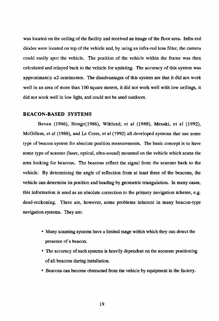
BEACON-BASED SYSTEMS
Bevan (1986), Hongo(1986), Wiklund, et al (1988), Mesaki, et al (1992),
McGillem, et al (1988), and Le Corre, et al (1992) all developed systems that use some
type of beacon system for absolute position measurements. The basic concept is to have
some type of scanner (laser, optical, ultra-sound) mounted on the vehicle which scans the
area looking for beacons. The beacons reflect the signal from the scanner back to the
vehicle. By determining the angle of reflection from at least three of the beacons, the
vehicle can determine its position and heading by geometric triangulation. In many cases,
this information is used as an absolute correction to the primary navigation scheme, e.g.
dead-reckoning. There are, however, some problems inherent in many beacon-type
navigation systems. They are:
• Many scanning systems have a limited range within which they can detect the
presence of a beacon.
• The accuracy of such systems is heavily dependent on the accurate positioning
of all beacons during installation.
• Beacons can become obstructed from the vehicle by equipment in the factory.
19

• Some systems require the vehicle to come to a complete stop in order to
determine its position.
• Extraneous light and sound sources can be erroneously interpreted as a beacon
by the vehicle.
• It is sometimes possible to have more than one position satisfy the angles
received from the beacons, i.e. triangulation may yield more than one result
• Conventional three-beacon systems have "zones" of high inaccuracy (see
Chapter 3, Figure 3.6).
Besides these problems, most beacon-type systems use the beacons as a secondary
navigation method, while relying on a different method, usually dead-reckoning, as the
primary method. The disadvantages of dead-reckoning navigation have been discussed in
Chapter 1 (Introduction).
Rathbone, et al (1986) used a system which combines sophisticated dead
reckoning with infrared beacons for absolute position measurement. In their system, the
vehicle is taught by being manually steered along the desired path. As the vehicle moves
about its environment, the vehicle records the positions of the beacons, which will be used
later for navigation. This allows arbitrary locating of beacons. The vehicle cannot detect
obstacles and change its course for obstacle avoidance. The camera mounted scans the
environment with a fish-eye lens, and is capable of detecting beacons up to 30 feet away.
The accuracy of the system is approximately three inches using beacons eight feet off the
ground. The advantage of this system is that the cost is low «S2500) and that precise
location of the beacons is not necessary. The main disadvantage of this system is that it
requires many beacons to be placed in the environment, and this prevents the system from
being feasible for outdoor applications. In addition, the system must be taught its path in
order to "learn" beacon positions.
20

Jarvis (1988) developed a control system used with a commercially available AGV,
the Denning DRV-1. Their system used a five-beacon system with an infrared scanner and
dead-reckoning to determine position and heading. As mentioned earlier, one of the
problems of beacon type positioning systems is that more than one position may satisfy the
angle measurements received from the three beacons. This problem is alleviated by
comparing the possible solutions with the estimate received from the dead-reckoning
system. The closest answer is selected as the most probable solution. In addition, five
beacons are used in the system to increase the possibility of seeing at least three beacons at
anyone time. A disadvantage is that the vehicle needs to come to a stop to determine its
position and that this calculation takes more than four seconds. In tests of the system, the
error was ±15 centimeters when tested in a 10 meter by 10 meter room. The heading error
was ±5°. As with other beacon referenced systems, the accuracy of this system is only as
good as the placement and calibration of the beacons.
Evans (1988) detailed one of the first commercially implemented autonomous
guided vehicle systems at Caterpillar. This system used bar-coded beacons and dead
reckoning. A laser scanner is used to read and identify the beacons, which are placed on
walls in specific locations. This vehicle is important because it was the first commercial
installation of a truly autonomous guided vehicle and showed that they could be cost
effectively implemented in industrial environments.
Both Nishide, et al (1986) and Tsumura, et al (1986) developed systems which
employed a laser transmitter and three "comer cube" beacons. Both systems determined
position based on the angular measurements of the reflections from the beacons. However,
neither system was able to calculate the position in real-time as the vehicle was moving.
The accuracy for Nishide's system was measured to be ±2 centimeters for position and ±5
arc minutes for heading. The maximum distance between the vehicle and anyone beacon
could not exceed 50 meters.
21

Tsumura's system worked with comer cubes which could be no more than 45
meters from the vehicle. Tsumura identified a triangle whose vertices were formed by each
comer cube (see Chapter 3, Figure 3). He found that the accuracy of the vehicle when it
was inside this triangle was much better than outside. Position errors were 5.7 centimeters
maximum inside the triangle and 14.0 centimeters outside the triangle. Heading errors
were 0.070 inside the triangle and 0.130 outside the triangle. One of the largest drawbacks
of both systems was the lack of real-time control.
VISION· AND MAPPING· BASED SYSTEMS
Frohn, et al (1989) developed a low-cost, high-performance vision navigation
system (VISOCAR) which worked in conjunction with bar-coded lane markings and
landmarks for position detection. In order to function properly, the AGV needed to operate
in a well-structured environment, it needed to operate within a plane containing these
elements, and a map of the terrain needed to be stored in the AGV's memory. For local
navigation, the vehicle recognized lane markings with its vision system and followed them.
Landmarks were placed at specific points and identified by the vision system to determine
location. The landmarks were represented in bar code for identification by the vehicle.
Although this system presented a cost-effective use of machine vision for navigation, the
successful implementation of such a system within a factory would require substantial
preparation to locate lane markings and landmarks. In addition, detailed mapping of the
area is required for navigation.
Cox (1991) also developed an autonomous robot vehicle which used local mapping
and dead-reckoning. The local mapping was performed by an optical range finder which
compared the current environment with that in memory to identify the environment. This
method was used to compliment the dead-reckoning navigation capabilities of the vehicle.
The advantage of this system is that it does not rely on beacons placed in the environment.
22

One of the disadvantages, again, is that it requires the user to create a map of the
environment before execution.
Gonzalez, et al (1992) presented a position estimator for a 2D laser range finder.
The system was based on the Carnegie-Mellon University Cyclone Locomotion Emulator,
which is an all-wheel drive and steer vehicle used as a testbed for robotics research. The
laser positioning system was able to scan at distances of up to 50 meters with a resolution
of ± 1 0 centimeters and an accuracy of ±20 centimeters. Testing was performed in a non
real-time environment with the vehicle moving one meter and then stopping to determine its
position. During testing the maximum position error was 3.6 centimeters with an average
of 1.99 centimeters. The maximum heading error was 1.8° with an average of 0.73°.
Cycle time to determine position was about two seconds.
CONCLUSIONS
All systems described here are autonomous systems which allow vehicle navigation
without the use of conventional techniques such as guided wire or tape. Many of these
systems are feasible from a cost standpoint, but others cannot be implemented in an
commercial system due to high hardware costs. With this in mind, these systems have
drawbacks which need to be improved upon before they can be useful to industry.
Some of the major drawbacks of these systems are:
Real-Time Navigation - Many of the systems would only be able to determine
the position of the vehicle after the vehicle came to a complete stop. To be
viable for industry, a vehicle must be capable of real-time, "on-the-fly"
navigation.
Site Preparation - Many of the beacon-based and mapping-type systems
require either extensive modification to or detailed mapping of the environment
23

to be stored in the vehicle's computer. In the case of beacons, the accuracy of
the system is dependent on the accuracy of the placing of the beacons.
Range .. No system which has been developed has a range of more than 50
meters for either scanning or position determination.
3-Dimensional Capability .. None of the systems discussed has dealt with 3D
positioning of a vehicle.
Dead-Reckoning - Most of the systems used dead-reckoning as the primary
method of navigation. As the areas of application for autonomous vehicles
move outside the highly structured and well-prepared factory floor, reliance on
floor condition will need to be eliminated.
This research will focus on these problems by developing an autonomous AGV
which can navigate in real time without the need to place beacons on the site. The system
will be able to go anywhere once the laser transmitters are installed and execute a pre
defined user path. The next chapter will describe the methodology and system used to
achieve this goal.
24

INTRODUCTION
CHAPTER 3 METHODOLOGY
The goal of this research was to develop and test the performance of an autonomous
automated guided vehicle which uses a laser-based positioning system as the primary
method navigation. The research work consisted of three major areas:
1. Path generation and navigation software development.
2. Hardware installation and debugging.
3. System testing and analysis of results.
The following sections describe the purpose of each of these areas and the steps
which will be followed for their development.
PATH GENERATION SOFTWARE
The path generation software converts a path drawn by the user to a format
understandable by the AGV. It acts as a post-processor between PC-based drawing
software (e.g. AutoCAD, CANVAS) that can export path data in the AutoDesk Drawing
Interchange File (DXF) format. The software converts this path to the necessary format to
be used by the vehicle for navigation. The DXF file format contains information which
describes the picture by using a text format containing X and Y coordinates for the
beginning and ends of polylines drawn by the user. This file is then analyzed by the post
processor and the coordinates for the path are extracted.
It is important that when the user draws the path, that there is a definite starting
point and an ending point with a continuous, connected series of line-segments. A
25

discontinuous path cannot be used because the AGV would not know how to get from the
end of one group of line segments (poly lines) to the next. In addition, the path cannot tum
back on itself. This would require the vehicle to move forward and then reverse its
direction. Since it is unclear to the vehicle when and how it should tum around, this
situation will not be considered in this research.
Figure 3.1a-c gives examples of valid and invalid paths. Figure 3.1a shows an
invalid path because it is discontinuous; Figure 3.th shows an invalid path because the
vehicle will be required to tum around on its path, requiring reverse travel or another
method. Figure 3.1c shows a valid path.
Start of Path ---...... ---
Discontinuous sadio
Figure 3.1a: Discontinuous Path Definition
Start of Path
Vehicle must double back on
its path here
Figure 3.1b: Invalid Turnaround in Path Definition
26

Start of Path ----...... ----
End 4-------.
Figure 3.1c: Valid Path Definition
For this research, software was developed which reads the contents of a DXF file
created by the user and extract X and Y coordinates for the desired AGV path. The
coordinates give the location of the end of each linear path segment. Since the AGV is not
capable of making a 90 degree tum, the intersections of each linear path segment must be
smoothed with an arc to allow the AGV to follow the transition from one path segment to
the other. The software, therefore, converts the path of straight line segments to a path
which connects the line segments by arcs for the AGV to follow. Figure 3.2 gives and
example of a path before and after blending arcs have been added. Notice that no arc needs
to be added to the upper left comer of this path since this is the start/end point and the
vehicle will not need to transition from the last segment to the first segment.
Start anq J:nd _ of Path ---------1-.....
-Before After
Figure 3.2: Path Before and After Adding Arc Transitions
27

After the path has been determined, the navigation program needs to transform the
X and Y path coordinates to wheel angle and velocity parameters. For the purpose of this
research, a constant velocity over the entire path is assumed. The navigation program
compares the desired position of the vehicle with the actual position of the vehicle from the
laser system and determines the appropriate adjustment to steering angle to remain on
course. A smoothing algorithm for the steering angle adjustment is also incorporated here
to control vehicle oscillation along the desired path.
The advantage of a graphical system such as this to describe the path is that the user
can quickly generate any path for the vehicle. In addition, the user can specify different
segment sizes, arc radii, etc. and determine their effect on vehicle performance. This was
very useful during system testing where it was necessary to-generate and test a wide variety
of paths and operating conditions.
HARDWARE INSTALLATION AND DEBUGGING
The system will consist of three main pieces of hardware with supporting software:
1. The laser-based positioning system.
2. A 386-based PC for navigation and path calculations.
3. The ISE Automated Guided Vehicle (AGV)
Laser-Based Positioning System
The laser based positioning system used in this research has been developed by
Spatial Positioning Systems, Inc. (SPSi) of Blacksburg, Virginia. The system consists of
three laser-transmitters located in the comers of the operating environment of the vehicle.
Position is measured from a receiver located on the vehicle. An optical sensor receives the
three laser beams from the transmitters and can calculate the receiver's X, Y, and Z position
using triangulation. Some of the advantages of this system are its high accuracy, fast
28

update rate, and range. The range of a new system under development is on the order of
250 meters, which far exceeds those of any other known system today. The system used
during this experiment, however, has a lower range than this. The positional accuracy of
the system is about 1 part in 100,000 (5 mm/SOO m accuracy) and the data transmission
(u¢ate) rate of the system varies from 4 to 100 Hertz.
During this research, only one receiver was used with the vehicle. The heading of
the vehicle wsd determined by finding the direction of a vector connecting the current
vehicle position with the previous known vehicle position. This heading vector was used
to determine if the vehicle was on course or not. Figure 3.3 shows the location of the
receiver on the vehicle. Using two receivers on top of the vehicle would have been
desirable. This would have allowed a more accurate and timely heading determination than
just one receiver.
Receiver
Vehicle
Figure 3.3: Receiver Mounted on AGV
The calculations for the }X)sitioning system are performed by an 80386 computer in
conjunction with the specially developed hardware used with the laser-based positioning
system. The software to calculate position has already been developed by SPSi and further
development of the system is not within the scope of this research. The }X)sitioning system
29

will communicate with the AGV system via an RS-232 Serial Interface, over which X, Y,
and Z coordinates of the vehicle will be transmitted. This information was received by
another 386 computer mounted on top of the vehicle. This computer and its software will
be described in the next section.
Hardware and Software for Trajectory and Path Calculations
A 386-based computer received the position information from the laser receiver.
This computer was the workhorse of the system and was responsible for sending the AGV
controlling computer updated steering angle commands. The desired path was determined
from the path drawn by the user using the graphical user interface. X and Y coordinates of
consecutive points along the path were constantly compared with the current position of the
vehicle and appropriate steering updates were calculated to keep the vehicle on course.
When the steering angle needed to be updated, the computer sent this information to
the AGV via AID boards within the computer and connected to the AGV's driving and
steering motor circuitry.
In conclusion, there were three main tasks for the 386 ("Host") computer:
1. To compute and compare the desired and actual trajectories.
2. To compute information that needs to be sent to the AGV to update its
trajectory .
3. To communicate this information to the vehicle.
The Autonomous Guided Vehicle
The vehicle used in this research is a dead-reckoning based vehicle designed and
built at the Department of Industrial and Systems Engineering at Virginia Tech. The vehicle
is a three-wheeled vehicle which used dead-reckoning as its primary navigation method.
30

The dead reckoning system on this vehicle is not extremely accurate, and that is why this
vehicle is very appropriate for this research. For this research, the dead-reckoning
capabilities of the vehicle were not used. As stated earlier, the purpose of this research was
to examine the effectiveness of using a laser-based positioning system as a navigation
means. This allowed the research to determine how well a vehicle can navigate when dead
reckoning is not possible.
The front wheel of this vehicle performs the steering and drive functions, while the
two rear wheels are not driven and cannot steer. For path following, a point at the center of
the front wheel was used as the vehicle reference point, as shown by Figure 3.4. This
point followed the path defined by the user.
I I
~Front Reference Point for Wheel
I I vehicle position
Figure 3.4: Reference Point on Vehicle
The vehicle was controlled by an 80386 computer which issued steering and
velocity commands and sent encoder information which described a trajectory. In this
system, the main 386-based computer communicated with internal NO controller boards to
control the motion of the vehicle.
Figure 3.5 summarizes the relationships between the various hardware and
software components of the system.
31

r------, I Positioning I I Sy&em I
I _______ J
N C")
N Raw Position Data en a::
r- - - -, I I I
Calculate X,Y,Z Position
I I SPSi 386 PC
_______ ...J
~ N
en a::
r------, I I Navigation
Software r------, I AID Boards I I
Calculate Updated Steering Angles
386 Host PC
I ~ Motors and I I Actuators
I __ ...J
AGV
Figure 3.5: Hardware and Software Diagram
32

SYSTEM TESTING AND ANALYSIS OF RESULTS
Testing of the system was based on how accurately the vehicle could move along a
path by comparing its actual position to its desired position on the path. In order to
examine system performance under a variety of conditions, four variables were used. The
variables and their possible states were:
Type of motion
a. Straight line
b. Cutvi-Linear (Straight line complex path with arcs between consecutive
linear segments)
Type of Path
a. Open-Loop ( Start pi! Finish)
b. Closed-Loop (Start = Finish)
Surface Quality
a. Smooth floor
b. Pavement
c. Poor floor quality (with conduits, oil, etc.)
Velocity
a. Slow «O.5m/sec)
b. Normal (1m/sec)
c. Maximum (unknown)
Another test was to examine the accuracy of the vehicle when it operated outside of
the triangle formed by the three laser transmitters. Tsumura, et al (1986) found that the
accuracy of a vehicle was worse when the vehicle was loCated outside a triangle whose
vertices are the locations of the laser transmitters/receivers. Figure 3.6 shows the two
areas. The gray area is the area where it is believed that accuracy may be higher.
33

Transmitter
Transmitter Transmitter
Figure 3.6: Region of Expected High Accuracy
The system was evaluated by comparing the vehicle's actual position to its desired
position. During testing, the software constantly recorded the position of the vehicle and
saved the coordinates to a data file. For analysis, this was then compared to the desired
path and a graph was produced comparing the two. In addition, the absolute average path
error at each measured position was calculated. For this research, the absolute average path
error is the absolute value of the perpendicular distance from the vehicle position to the
desired path.
During testing, navigation parameters were varied to determine how they affected
navigation performance. However, the goal of this research was not to statistically analyze
the effect of these parameters on navigation performance. This could be left as a future area
of research.
34

It was expected that by using a laser-based positioning system as a navigation
method for a vehicle, that the vehicle would be able to successfully navigate a given path
described in the navigation computer's memory and that the absolute average path error
would not exceed 20 centimeters.
35

INTRODUCTION
CHAPTER 4 PATH GENERATION
For an AGV to move about a workspace, it must have some defined path to follow.
In conventional AGV systems, this path is usually defined by an embedded wire in the
floor or magnetic/optical tape. One of the advantages of autonomous AGV systems is that
the path is not defined by a wire or tape, but rather in the memory of the computer, either
on the AGV or off-board. Because the path does not physically exist on the factory floor,
it can be modified through software, thus reducing the time and effort required for path
modification.
To exploit the advantages of autonomous AGV path definition, it was decided to
allow the user to define the path graphically on a computer screen. This graphical approach
allows the user to easily define the path and to see what shape the path will be. A post
processing program then converts the drawing of the path into a path description which the
AGV can understand. The purpose of the path generation software developed for this
research is to allow the user to draw a path on a computer screen and to convert that path
into a format which can be used for vehicle navigation. This graphical user interface was
especially useful when testing the vehicle. The software allows rapid modification and
generation of new paths to facilitate testing of the vehicle.
METHODOLOGY
Drawing Interchange File Format
To generate a path, the user must use a graphics program to export picture data in
the AutoDesk Drawing Interchange File (DXF) format. Some example programs with this
capability are AutoCAD for DOS-compatible computers and CANVAS for Macintosh
36
computers. See the AutoCAD Reference Manual for more information about the DXF file
format.
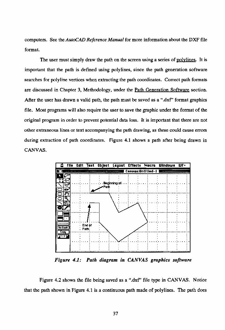
The user must simply draw the path on the screen using a series of polylines. It is
important that the path is defined using polylines, since the path generation software
searches for poly line vertices when extracting the path coordinates. Correct path formats
are discussed in Chapter 3, Methodology, under the Path Generation Software section.
After the user has drawn a valid path, the path must be saved as a ".dxf' format graphics
file. Most programs will also require the user to save the graphic under the format of the
original program in order to prevent potential data loss. It is important that there are not
other extraneous lines or text accompanying the path drawing, as these could cause errors
during extraction of path coordinates. Figure 4.1 shows a path after being drawn in
CANVAS.
File Edit TeMt ObJett Leyout Effeet. Mecro Window. WF+
Cenue.:Untltled-1
" .. . .. , ., ~~-ft, , , ,', •• , : ••• ,' •• Be~nning.of ... : .... ' .... : •..• ' ..•• : •..• ' •... : . . ~ /P8~ . i . ~ . ~ . : o e-; :..,-.: : : : . o ................. ········· .. · .. · .. ~ .... ···· ...... · .. r .... · .. · .. · .. ···~ ...... ····· ...... ~ .. o . l 1 l l ~ + , ... :.. .. . -:' . , 'j' ,. , ... ~ , , .. > .. '1" .. : .. , '1'
D~ ·"·····:·"···t~········ .. ·l .. · .... · .... ·· .. ·l .. ·· .. · .... · .... ·~ .. ~D : i ~ . 1 . j r::::::=I .•..... ....• . •.....•........... ~-- : End~f : . : . : INoDashl . p .... ; . : :
• aUI. • .:: c:§J ·· .. · .. ·:· .. · .... l········:·· ...... ; ............ : ................. : ................. : ..
[illJi .... : .... i .... : ... ·1· . . . .. ! ... -: .... : .... ;. ... : .... ;. .... . .. .... .. . .. .. .. . . . . . ............................................ , ... ' ..... ,., ........... , ........................................ ,
Figure 4.1: Path diagram in CANVAS graphics software
Figure 4.2 shows the file being saved as a ".dxf' file type in CANVAS. Notice
that the path shown in Figure 4.1 is a continuous path made of poly lines. The path does
37

not double back on itself and has a clear beginning and end. Although this is an example of
an open loop path (STARTpltEND), it is also valid to have a path with the starting point the
same as the ending point.
,.
. . ~Io--=-d •••• : •••• j .... :- ... ; .... : .... ! .... : .... ! ... : ... ! ... : ... ! ... : .... ! .... : ~1:::Jord"""""""'" ~ ~~~~~~"'~~~~"'~~~~"'~~~~~~'~"'~~:~~""':"'''''T'' ····~·······r··· .. ·j ..
1~~luo:uuuuuo::~o leThe ••• D ••• ' ~ I:.:::' t:uO:r:u:J:uou::u
· . . . .. .. . . . .. Is .... uU./du;;:.t documont II' I[ Slue I] 10
0 0 0: 0 0 •• i .... : .......................... . u "Cancel ............... ..
File For •• t: ... 1 _DH_F ___ _ • •••• ~ ~ 4 4 • • • • 0 trilete a.ekap File .......... .
. . ........ : ........ : ........ : ........ j ••.••••• : ....... ·l····· ... : ........ ~ ........ : ........ ~ ........ : ........ 1·· .... · .. · ...... ,·: .. · " ...... .
· ... ~ .... ! .... ; .... 1 .... ; .... ! .... ; .... J .... ; .... 1 .... ; .... 1 ... ':' .. .
Figure 4.2: Saving the drawing as a ".dxf" file in CANVAS
Appendix A shows an example of a file in the "DXF' file format. Most of the
information in this file will be ignored by the path generation software. The important
pieces of information in the DXF file are the coordinates of the polylines in the drawing.
The DXF file will give the coordinates of each vertex on the path. The following listing
shows a sample part of the DXF file containing the vertex information:
38

(previous statements)
70 o
o VERTEX
8 LAYERl
10 3 20 7 30 o 42 o 70
o o
VERTEX 8
LAYER 1 10 2 20 9 30 o 42 o 70
o o
SEQEND o
END SEC
From this sample piece of DXF code, the line "VERTEX" indicates that the
coordinates of a new vertex are going to be listed next. "LAYERl" indicates on which
drawing layer the vertex is located, in this case, layer number one. The next six numbers
give the X, Y, and Z coordinates of the vertex. The X coordinate is proceeded by a "l 0",
the Y coordinate by a "20", and the Z coordinate by a "30." This sample text gives two
39
vertex coordinates. In this case the coordinates would be X=3, Y=7, z=o for the first
vertex and X=2, Y=9, z=o for the second vertex. Using these rules, the program scans
the DXF text file for the word ''VERTEX'' and then extracts the X and Y coordinates for that
vertex. For this research, the Z coordinate is not used. However, future research using
three dimensions could easily extract any Z-axis coordinate information.
When defining the path, the path generation software assumes that the order in
which the vertices appear in the DXF file is the same order in which they appear on the
path. For this reason, it is important that the user draw the path in the correct order in order
to avoid confusion and/or incorrect path generation.
Arc Blending
As mentioned in the methodology section, the vehicle is not capable of turning a
sharp angle, such as that found at the intersection of two linear path segments. For this
reason, it is necessary to blend linear path segments with arcs. This will allow the vehicle
to smoothly transition from one linear path segment to the next.
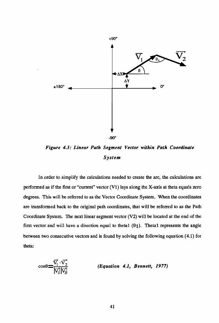
In order to blend two linear segments with an arc, the angle between the
consecutive vectors must be known. Figure 4.3 shows the untransformed linear segment
and its angle, theta, with the X-axis as well as the numbering convention used to assign a
value to theta. All vectors whose direction points in the third or fourth quadrants have a
theta value which is negative.
40
flY
±180°
Figure 4.3: Linear Path Segment Vector within Path Coordinate
System
In order to simplify the calculations needed to create the arc, the calculations are
performed as if the first or "current" vector (V1) lays along the X-axis at theta equals zero
degrees. This will be referred to as the Vector Coordinate System. When the coordinates
are transformed back to the original path coordinates, that will be referred to as the Path
Coordinate System. The next linear segment vector (V2) will be located at the end of the
first vector and will have a direction equal to theta1 (81). Theta1 represents the angle
between two consecutive vectors and is found by solving the following equation (4.1) for
theta:
(Equation 4.1, Bennett, 1977)
41

Using the above mentioned convention, the two vectors will appear as in Figure 4.4
in order to calculate the arc between the two.
y
~----~------~~~--------------~x
Figure 4.4: Untransformed Segment Vectors in the
Vector Coordinate System
To create an arc between the two lines the radius of curvature, p, of the arc must be
calculated. Within the DXF file, the coordinates for the path are given with an X value
between 0 and 7.5, and a Yvalue between 0 and 10.5, which corresponds to coordinates
of a piece of paper with the origin in the lower left hand corner of the page. When the path
generation program extracts the path coordinates, the user has the option of multiplying the
path by an X and Y scaling factor, kx and ky, respectively. The magnitude of the radius of
curvature of the arc will be dependent on this scaling factor. Equation 4.2 is used to find
the radius of curvature. Notice the radius scaling factor, K, which can also be modified by
the user as needed to make a larger or smaller radius of curvature.
42

(Equation 4.2, Adapted from Cox and Nelson, 1990)
Once the radius of curvature is found, the point of intersection of the arc and the
vector must be found. This is the point where the path must make the transition from the
linear segment to the curved arc. This distance, d, is found from Equation 4.3.
(Equation 4.3)
To determine whether the arc will be above or below the current vector, the
program simply compares the Y-coordinate of the end-points of the two arcs. If the Y
coordinate of the end-point of the second vector is less than that of the first vector, this
indicates that the second vector points "down" with relation to the first vector. Therefore,
the arc should be drawn below the first vector to connect the two. The converse holds if
the arc is to be drawn above the first vector. Figure 4.5 shows this relationship and the
location of the arc.
Arc drawn below first vector
Figure 4.5: Location of Arc
43

In this example, since Y2 has a lower value relative to Yh the arc is drawn under or
below the first vector. It is important to realize that the vectors are compared to each other
relatively, and not absolutely. This is because the absolute Y-coordinate of the second
vector could be greater than that of the first vector, but be lesser relative to the first
untransformed coordinate. Before the first vector is transformed back to the path
coordinate system, the Y -coordinate of the end-point of the first vector is always zero.
Path Segment Generation
After the radius of CUlVature and the location of the arc has been established, the arc
must now be added to the path between the two vectors. Due to the method of navigation
used, the path is broken up into many small segments. Chapter 5, Navigation, will give
more details on why this is so. In order to be of use to the navigation software, the path is
described as a series of points which describe the path. These points are then followed by
the vehicle during navigation. It is worth noting here that each arc is broken up into a
series of linear segments. Therefore, the vehicle does not navigate a circular arc, per se,
but rather, moves along a series of line segments which approximate an arc. Figure 4.6
shows an example of a path before and after path generation by the software.
As can be seen from Figure 4.6, each original poly line segment and the arcs are
reduced to many small path segments. During navigation, the vehicle will move along the
path following these small path segments. The size of these segments can be modified by
the user with the path generation software.
44

700
600
500
400
300
200 o Original Path C After Arc
Blending and Path Genertion
100 200 250 300 350 400 450 500 550 600 650 700 750
Figure 4.6: Path Before and After Arc Blending
At this point, the path generation software has calculated the arc between two
vectors and then broken this path into small path segments. However, when the vector and
arc are computed, they are computed in the vector coordinate system, with the beginning of
the first vector at the origin and the direction equal to zero degrees. The software must now
take all of the path points and transform them back to the original path coordinate system.
This is done each time a vector and the corresponding path points are generated, not after
the entire path has been generated. The following formula is used, where X and Y
45

represent the path coordinates and X' and Y' represent the path coordinates in the vector
coordinate system.
X = X'cos9 - Y'sin9+ AX
Y = X'sin e + Y'cos 9 + A Y (Equation 4.4)
In Equation 4.4, the angle Theta (9) is the angle of the current path vector in the
Path Coordinate System. Delta X (AX) and Delta Y (A Y) represent the beginning X and Y
coordinates of the current vector in the Path Coordinate System.
PATH GENERATION SOFrWARE
The path generation software is menu driven to allow easy modification of path
generation parameters and path generation. Upon initial execution of the program, the user
will see the menu shown in Figure 4.7.
PATH GENERATION MENU C)hange Parameters G)enerate Path Q)uit
PARAMETERS Input File: AGV7.DXF Output File: PATH7.DAT X Scaling Factor: 100.000 Y Scaling Factor: 100.000 Path Segment/Step Size: 50.000 Radius of Curvature Multiplier: 0.300
Enter Selection (C, G, or Q):_
Figure 4.7: Path Generation Software Main Menu Screen
46

Main Menu Options
The user has three options from the main menu:
Chan"e Parameters ("C'):
This option allows the user to change any of the options which are listed under
"PARAMETERS" on the main menu. These parameters are described below in the Change
Parameters Menu section.
Generate Path ("G"):
If the user is satisfied with all parameter values, then path generation may begin.
The path description data is read from the input file specified and saved in the output file
specified. Be sure to include the path to the input file if it is located in a separate directory.
If the program can locate and open the input file, it begins extracting the path coordinates.
Mer the path vertices are read, the program displays how many points were read from the
path. The calculations for path generation are then performed and a message is displayed
saying that the final path is being saved in the output file. After this step, the user may exit
the program and begin vehicle navigation using the navigation software.
Ouit Promm ("0"):
This option will exit the program. All parameters are saved in a preferences file on
the current directory under the name "path. prf". The user must make sure this file is on
the current directory when running the program or an error may occur.
Change Parameters Menu:
If the user selects the Change Parameters option ("C") from the menu, the
following menu shown in Figure 4.8 is displayed.
47

PARAMETERS 1) Input File: AGV7.DXF 2) Output File: PATB7.DAT 3) X Scaling Factor: 10.000 4) Y Scaling Factor: 10.000 5) Path Segment/Step Size: .500 6) Radius of curvature Multiplier: .3000 7) Return to Main Menu
Enter Selection (1 - 7):_
Figure 4.8: Change Parameters Menu in Path Generation Software
The following will describe each parameter:
1) Input File:
The Input File is the name of the original Drawing Interchange File (D XF) format
data file which has been generated in another graphics program (CANVAS, AutoCAD,
etc.). It is very important that this file is a text file containing DXF picture information. If
not, the program may behave unusually and crash.
2) Output File:
The Output File is the file which will be created by the path generation software.
This file will be read by the navigation program during path navigation. For this reason,
this file name should be specified as the input file when running the navigation software.
This file will contain the (X, Y) coordinates of the path segments.
48

3) X-Scalin~ Factor:
The original DXF polyline x-coordinates will be multiplied by this factor when
generating the path. The effect of this will be to shrink or expand the path according to the
user's desire.
4) Y-Scalin~ Factor:
The Y-Scaling Factor has the same effect as the X-Scaling Factor, except it is
applied to the Yaxis. It is important to realize that if the X- and Y-Scaling Factors are not
equal that the aspect ratio of the original path will be lost.
5) Path Se~ment! Step Size:
The Path Segment/Step Size determines the length of a path segment for the
finished path. The smaller this number, the more segments the path contains.
6) Radius of Curvature Multiplier:
The Radius of Curvature Multiplier parameter determines the relative size of the arc
which connects two line segments. A larger value results in a larger radius of curvature
and visa-versa.
The user can also return to the main menu by selecting option "7". After the user
changes a parameter, the program will automatically return to the main menu. As
mentioned earlier, all parameter values are saved in a data file to disk when the user exits
the program.
49

CONCLUSIONS
Using the path generation software, the user has the ability to quickly create and
modify AGV paths. The software reads the contents of a Drawing Interchange Format
(DXF) file containing the path information in the form of polyline data. Using any
convenient graphics software which can export picture data in DXF format, the user can
draw the desired AGV path. The path generation software exploits one of the advantages
of autonomous AGV systems, that is, the ability to modify paths easily. Because the path
is stored in computer memory, no physical modification to the workspace is necessary.
During testing of this system, this was very useful for testing different paths for the AGV
to follow. A listing of the path generation program code is shown in Appendix B.
50

INTRODUCTION
CHAPTER 5 NAVIGATION
After the user has created a path and generated a path output file using the path
generation software, the vehicle is ready to navigate the path. The objective of the
navigation is to have the vehicle follow the path specified by the user. The coordinates of
points along the path are stored in the output file specified by the user. The navigation
software allows the vehicle follow these points and correct any path error in real time as the
vehicle is moving. This chapter will outline the methodology and describe the navigation
software used to navigate the vehicle.
METHODOLOGY
As outlined in the path generation chapter, the input file for navigation contains a
list of points which describe the path. The distance between each point is specified during
path generation as the path step/segment size. During navigation, the vehicle determines its
path by determining the next path point corresponding to its position and heads towards it.
This is in contrast to having the vehicle determine how far it is away from the path
measured by, for example, perpendicular distance and correcting for the error. Referring to
Figure 5.1, if the vehicle was at the beginning of the path, PI, the vehicle would look
down the path to the next point, P2. The vehicle then heads in that direction. When the
vehicle receives a position update from the laser-based positioning system, the software
determines whether the vehicle is still heading towards its goal point or not. If it is not, a
steering adjustment is made and the vehicle continues.
51

names:
Size r Segment .1 •• t------t ...... ---•• t-----t ........ path P1 P2 continues
Figure 5.1: Path Points
In order to explain the navigation methodology, assume the following variable
Theta (6) : Angle of vector between last goal point and current goal point
ThetaAGV (6 AGV) : Measured heading of AGV
Theta2 (62) : Angle of vector between current AGV position and current goal point
DeltaTheta( A9): Heading error between actual AGV heading (9 AGV) and
desired heading (62)
Figure 5.2 shows each of these variables.
Previous -goal Current AGV position point
9
pat~ " dire~io~
Figure 5.2: Angle Conventions for Navigation
52

During navigation, the position and heading of the AGV were updated by the laser
based positioning system. The software then calculated the angle DeltaTheta(A8) between
the AGV and the current goal point. This angle was compared to the current AGV heading
and a steering correction was made if necessary. The heading of the vehicle was
determined by calculating the angle of a vector connecting its present position and its last
measured position. This method gave a good approximation of vehicle heading, although
the heading could have been more accurately determined with two receivers mounted on the
vehicle. Two receivers would have allowed an instantaneous heading calculation and
would have beeen more accurate in that the heading could have been determined by the
direction of a vector connecting the two receivers. The amount of steering correction was
determined by the angle to tum the wheel and the amount of time to apply the steering.
Both of these parameters can be modified by the user with the software. These parameters
are important to avoid over correcting the AGV during navigation.
Another important issue is when to change goal points on the path. This can be
done by determining how far the vehicle has traveled along the current vector connecting
the last goal point and the current goal point. To do this, a perpendicular line is constructed
from the AGV position to the vector between the two path points. The distance between
the intersection of this point and the last goal point is then measured. This distance, call it
xdist, is then compared to the overall length of the vector between the last and current goal
points. If it is greater than or equal to some threshold percentage of the overall length, then
a new current goal point is read from the path file and the current goal point becomes the
previous goal point. The vehicle now heads for the new goal point. Figure 5.3 illustrates
this concept.
With the software, the user can modify the threshold percentage along the vector. It
is expected that this would also affect the navigation characteristics of the vehicle.
53

Previous -goalpoint
Figure 5.3: Determination of AGV Position Along Vector Connecting Two Path Points
NAVIGATION SOFrWARE
The navigation software was designed to allow the vehicle to navigate any path
generated using the path generation software. The input file for the navigation software
must be generated from the path generation software in order to execute a path. As with the
path generation software, the navigation software is menu driven to allow the user to easily
modify parameters and navigate the vehicle. Figure 5.4 shows the main menu screen for
the navigation software.
Main Menu Options
The user has three options from the main menu:
Change Parameters ("C'):
This option allows the user to change any of the options which are listed under
"PARAMETERS" in the main menu. These parameters are described below in the Change
Parameters Menu section.
54

NAVIGATION MENU C)hange Parameters B)egin Navigation s)imulate Navigation Q)uit
PARAMETERS Input File: PATH7.DXF AGV Speed (m/s): 1.000 Maximum AGV Speed (m/s): 2.000 smoothing constant: 1.000 Max. steering Activation Time: 1.000 Threshold Percentage: 50% simulation Update Rate (sees): 1.000 position Record File Name. OUT7IA.PTS Error Record File Name: ERR71A.DAT
Enter Selection (C, B, S, or Q):_
Figure 5.4: Main Menu Screen for Navigation Software
Be~in N avii3tion ("N"):
By choosing this option, the program begins navigation of the vehicle. The vehicle
does not start moving until the break relay on the vehicle is activated and the emergency
stop switch is disengaged. The vehicle then follows the path as described in input file.
When the vehicle is finished the path, the program returns to the main menu.
Simulate Navi~ation ("S"):
The simulation option of the software simulates the navigation of the vehicle
without using the laser-based positioning system. The main purpose of the simulator is for
debugging of the navigation software during development. For future development work,
the simulator would be useful.
The simulator works by assuming the vehicle starts at the beginning of the path.
The simulator then waits a specified period of time (equal to the Simulation Update Rate)
and then calculates a new position based on the desired speed of the vehicle, the direction
of the vehicle, and the time of the Simulation Update Rate. A random error is then added to
55

the X and Y coordinates of the vehicle. The navigation software then proceeds with
navigation as if this new position were input from the laser based positioning system. This
process continues until the entire path has been traversed.
By modifying the program code, the simulation can be run with the dlive motor and
the steering motor either on or off. For this research, the driver motors were turned off and
the steering motor was kept on. One of the sources of approximation of the simulator is
determining the calculated position of the vehicle after turning the wheel some angle for
some period of time. The values arrived at were approximations at best and did not model
the actual position of the vehicle with enough accuracy to allow the vehicle to move along a
path during simulation. This may be an area to be looked at in future research.
After the simulation run, a data file ("EVENTDAT.DAT") exists which describes in
detail all navigation events which occurred during the simulated navigation. The following
shows a sample simulation run:
Read path point: x=66.669998 y=933.3300l7 Read path point: x=86.669998 y=933.3300l7 AGV position: x=8l.574493 y=932.242493 dir=-4.l73383 Read path point: x=106.669998 y=933.3300l7 xdist=-5.095505 d=20.000000 phi2=2.481567 Turn AGV 6.654644 deqrees for 0.400000 seconds ••• Newaqv.dir=-1.709729 AGV position: x=96.634926 y=93l.440186 dir=-3.049498 xdist=9.964928 d=20.000000 phi2=10.665968 Turn AGV 13.714590 deqrees for 0.400000 seconds ••• New aqv.dir=2.104058 AGV position: x=lll.279488 y=932.33l360 dir=3.482463 Read path point: x=126.669998 y=933.330017
In this example the simulator first read two path points: (66.67,933.33) and
(86.67,93.33). It then generated a new AGV position of (86.57,932.24). The heading of
the AGV was determined by calculating the angle between the current AGV position and
the previous AGV position. In this case, the previous AGV position was the beginning of
56
the path at (66.67,933.33). For this simulation the threshold percentage was 50%, and the
program reads a new path point because the vehicle is more than 50% along the distance
between the two current path points. The simulator now shows some calculations
concerning the position and desired heading of the AGV. From these calculations it is
determined that the AGV needs to tum 6.65 degrees for 0.4 seconds (the steering activation
time). A new heading which resulted from this steering correction is calculated and the
program repeats the process again until the path is traversed. The information saved in the
"EVEN'IDAT.DAT" file can be modified to suit the needs of the developer by changing the
original program code.
Ouit Promm ("0"):
This option exits the navigation program. All navigation parameters are saved in a
preferences file on the current directory under the name "nav.prf." Make sure this file in
on the current directory when running the program or an error may occur.
Change Parameters Menu
If the user selects the Change Parameters option ("C") from the main menu, the
menu shown in Figure 5.5 is displayed.
The following is a description of each parameter:
1) Input File:
The Input File is the name of the file created by the path generation software. This
file contains a list of points which describe the path the vehicle must follow. These points
represent each vertex of the path when the path is broken up into line segments of length
equal to the step or segment size as designated by the user in the path generation program.
57

In addition, the header of this file tells the navigation program how many points are in the
path point list.
PARAMETERS 1) Input File: PATB7.DXF 2) Vehicle Speed (m/s): 1.000 3) Maximum Vehicle Speed (m/s): 2.000 4) Smoothing Constant: 1.000 5) Time to Apply Steering: 1.000 6) Threshold Percentage: 50% 7) Simulation Update Rate (sees): 1.000 8) position Record File Name: OUT71A.PTS 9) Error Record File: ERR71A.DAT 0) Return to Main Menu
Enter Selection (0 - 9):_
Figure 5.5: Change Parameters Menu for Navigation Software
2) Vehicle Speed:
The Vehicle Speed is the speed, in meters per second, that the user wishes the
vehicle to travel. During path traversal, the speed of the vehicle will remain constant.
3) Maximum Vehicle Speed:
The Maximum Vehicle Speed is used to determine what value to send to the AGV to
achieve the correct speed. This value should not change after the maximum vehicle speed
has been determined. This value should not be used to increase or decrease vehicle speed.
4) Smoothing Constant:
The Smoothing Constant parameter tells the AGV how many degrees to correct its
steering by when a course correction is necessary. The angle to tum the AGV is equal to
the smoothing constant multiplied by the heading error. For example, if the AGV heading
58

error was 45° and the smoothing constant was .5, the AGV would turn its wheel 45° x 0.5
= 22.5°. The effect of this is to control the response of the vehicle to prevent over- or
under-correcting during navigation.
5) Steering Activation Time:
The Steering Activation Time specifies how long to apply the calculated steering
angle before returning the wheel to the straight ahead position. This time is specified in
seconds. As with the smoothing constant, this parameter will tend to either smooth or
increase the response of the vehicle during navigation.
6) Threshold Percentage:
The Threshold Percentage determines when the software should read the next goal
point on the path for the vehicle. The distance the vehicle will travel towards anyone point
is the distance between the current goal point and the previous goal point multiplied by the
threshold percentage. For example, if the threshold percentage is 50%, then the vehicle
will head towards the current goal point as long as it has not passed the half-way point
between the current goal point and the previous goal point. If the vehicle is past this half
way point, then the next path goal point is read and the vehicle heads towards it. Figure
5.3 diagrams this concept. As the threshold percentage increases, xdist will increase, and
visa-versa.
7) Simulation Update Rate
The Simulation Update Rate is the time, in seconds, that the simulation program
will pause before calculating another position for the AGV.
59

8) Position Record File Name
The Position Record file records the position of the AGV which is received from
the laser-based position system as the vehicle traverses the path. This is useful for plotting
a graph showing the course of the vehicle compared to its desired path.
9) Error Record File Name
This file contains the perpendicular path error of the vehicle every time it receives a
position update. The errors are always positive and the file also gives the average error at
the end of the listing.
The user can also return to the main menu by selecting option "0". After the user
changes a parameter, the program automatically returns to the main menu. As mentioned
earlier, all parameter values are saved in a data file to disk when the user exits the program.
CONCLUSIONS
Using the navigation software, the vehicle is able to follow a path originally
specified by the user as a DXF-format file. The navigation software reads a path data table
which is created by the path generation software. This path information is then used for the
real-time control of the vehicle around the path. The software allows the user to modify
the vehicle speed, as well as other parameters which control the response charactetistics of
the vehicle. This ability will allow for testing under a variety of conditions to determine
which combination of parameter settings provides the best performance for the vehicle. In
addition, the software allows the user to simulate path navigation for testing purposes and
to save point and path error information to data files for later analysis. A listing of the
navigation software program code is shown in Appendix C.
60

Chapter 6 RESULTS AND DISCUSSION
After the navigation and path generation software had been written and debugged,
the next step in the research was to test the vehicle with the laser-based positioning system.
Two problems which arose prior to testing were allocating the laser-based positioning
system from Spatial Positioning Systems, Inc. and finding an area large enough to set up
the system and run tests with the vehicle. Testing was performed over the weekend of
April 23-25, 1993 at Virginia Tech's Corporate Research Center. The testing area used
was in a newly constructed office building which had a large open area with a smooth
concrete floor. Since the building was new, the floor spaces had not yet been separated
into individual offices.
SYSTEM SET-UP AND CALIBRATION
Approximately half a day was needed to move the equipment from SPSi
headquarters to the test site, set-up the transmitters, and calibrate the system. The laser
transmitters were located at three comers of the testing room as shown in Figure 6.1. The
laser receiver and associated hardware were mounted on the vehicle, along with a 386-
based computer to calculate position and another 386-based computer to control and
navigate the vehicle. A serial cable was used to connect the receiver hardware to the
computer to calculate position, then another serial cable sent the position coordinates to the
navigation computer. Due to problems with the batteries, an extension cord was used to
power the computers, although the vehicle's motors still ran off the 12VDC batteries on
board. It was also suggested by the SPSi engineer to cover the windows of the room with
61

white plastic sheeting in order to reduce the possibility of multipath interference from
sunlight.
After the system was set-up and running, the system was ready for path testing.
The goal of the research was to demonstrate that a vehicle could navigate a path using the
laser-based positioning system as its only means of navigation. Therefore, it was decided
to use a variety of different paths and to observe how well the vehicle could follow the
path. It was also decided to see how the changing of navigation parameters affected the
navigation of the vehicle.
For reasons which will be described later, three separate path shapes were used: a
straight line path, a path consisting of two line segments, and a path consisting of three line
segments.
Laser #3 0
~ ~ "'0 a ~ \0
8 ('I)
n ;J
y
o Laser #2 Laser #1
.... Approx. 9 meters
Figure 6.1: Layout of System During Testing
62

Within this system, the origin of the laser system's coordinate system was at the
middle of Laser #1. The X-axis was represented by a line connecting the center of Laser
#1 to the center of Laser #2. The Y-axis was located perpendicular to the X-axis in the
direction of Laser #3, but not necessarily running through the center of it
TEST RESULTS
The next step was to perform the actual testing of the vehicle with the laser system.
The following sections will describe each test and the parameters used for the three paths.
All measurements used in testing are given in centimeters. The laser system returned
position coordinates in millimeters, and this number was simply divided by ten to give the
position expressed in centimeters. For each test, the vehicle was placed near the starting
point of the path and navigation was begun. When the vehicle reached the end of the path
the vehicle stopped and the test was concluded.
Test 1: Straight Line Path
For the first test, a straight line path was used. Figure 6.2 shows the coordinates
and location of this path within the work area.
For Path 1, the starting point was x=250 centimeters, y=200 centimeters. The
ending point of the path was x=250 centimeters, y=700 centimeters. The tests were
labeled la, Ib, 1c, etc. Most of the tests were run in groups of three or four. That is, the
same parameters were used for three or four runs, then some parameters were changed,
three or four runs were made again, and so on.
63

Laser #3 o
(250,700)
o Laser #1
(250,200) o Laser #2
Figure 6.2: Path #1
Tests la, lbe lc, ld:
Tests la, lb, lc and ld were run with the same parameters. They were:
Speed = 0.20 (Maximum = 1.00)
K (Smoothing Constant) = 1.0
Steering Activation Time = 0.4 seconds
Threshold Percentage = 50%
Path Segment Size = 100 centimeters
For all tests the speed was expressed as a percentage of the maximum speed. For
example, since the maximum speed was 1.00, this represented the fastest the vehicle was
64

capable of traveling. The speed used in testing was .20, so the speed of the vehicle was
20% of its maximum speed.
Tests 1a and 1d were very similar to each other. The vehicle began the path slightly
to the left of the path and headed towards the path, demonstrating that the navigation was
working. As can be seen from Figure 6.3, the vehicle usually stayed slightly to the left of
the path. It is believed that this was due'to a slight misalignment to the left of the steering
wheel of the vehicle. This caused the vehicle to naturally be to the left of the line.
700
600
500
400
300
Recorded..... ....Path 200
o 50 100 150 200 250 300 350 400 450 500 Path (x)
Figure 6.3: Results of Test la
One problem that was noticed during the first test was that at the beginning of the
path traversal, the vehicle would receive position updates in rapid succession without ever
65

moving. Since the heading of the vehicle is computed by determining the angle between
two consecutive position updates, the navigation software was calculating incorrect
headings. This was because it would either try to calculate the angle of a vector with no
length, or because two points would be so close to each other that the heading which was
calculated had no relationship to the actual heading of the vehicle. For this reason, the
navigation software was changed to require that the vehicle traveled at least five centimeters
between position updates. This effectively solved the problem.
As mentioned earlier, tests 1a and 1d were very similar. For this reason, test 1a is
shown in Figure 6.3 for clarity. The absolute average error for test 1a was 5.5 centimeters.
For test 1d, the average error was 2.95 centimeters. These errors are considered to be
acceptable for path navigation by the researcher.
~
i 0..
700
600
500
400
300
200
System began returning valid updates again at
this point (
----..\ -4-PaIh
Recorded,.....J' > "
I
Bad Position Updates Here
o 50 100 150 200 250 300 350 400 450 500 Path (x)
Figure 6.4: Results of Test Ib
66

The results graph plots the actual position of the vehicle versus the desired path.
Although tests la and Id had good results, tests Ib and lc were different. Figure 6.4
shows the results of test lb.
From the figure, it would appear as if the vehicle deviated wildly from the path in
the beginning and the middle of the path, and then got back on track towards the end. This
is not actually what happened, however. With this system, the laser-based positioning
system sent updated position estimates of the vehicle to the navigation system. The
navigation software then used this infonnation to determine whether or not the vehicle was
on course. In order for the navigation software to function correctly, it is important that the
laser-based positioning system gives correct position updates to the system. At times,
however, the positioning system did not return valid data to the navigation software, and
this was a frequent cause of navigation error. During navigation for Test Ib, for example,
the positioning system told the vehicle it was to the right of the path when it was actually
just to the left of the path. These false coordinates were then saved in the path point record
file. The first hump at the beginning of the path shows the vehicle off to the right,
however, at this point the vehicle was actually just to the left of the path. Since the
navigation software thought the vehicle was to the right of the path it told the vehicle to tum
left to get back to the path. This resulted in the vehicle traveling even further to the left of
the path.
When the positioning system began returning valid updates, the vehicle was then
approximately 25 centimeters to the left of the path. At this point the navigation software
needed to correct the vehicle again, but to the right to get back on the path again. It can be
seen that the vehicle did begin to get back to the correct location at the end. The absolute
average path error for test Ib was not a valid value because it did not really convey the
actual position of the vehicle, but rather took invalid position updates into account. Test Ie
also had much the same problem as Ib with errors from the positioning system.
67

Tests Ie, If:
Tests Ie and If were run with the same parameters as the first four tests except the
speed of the vehicle was increased to .25 of maximum. Figure 6.5 shows the results of
test Ie.
700
600
500
300
200
o
Badpoints ./ from positioning
.-\~
100 200 300 Path 1 (x)
400 500
Figure 6.5: Results of Test Ie
600
The reader will note from the graph that there are some points which appear to be
incorrect. These points were caused by the positioning system returning only one bad
point at a time. This is in contrast to test Ib where the system seemed to "drift" to the right
with its position data. In test Ie, the system gave two bad points at the beginning and a
couple at the end. However, because these points were isolated, their effect on navigation
was minimal and did not really alter the course of the vehicle. In order to show how the
68

system actually behaved, it is necessary to manually edit out the invalid positions from the
point record data file. In this case, test If also had the same type of problem as test Ie.
800
700
600
400
300
200
Recorded (1e)
100p-------------------------------------------+ -100 o 100 200 300 400 500 600 Path 1 (x)
Figure 6.6: Results of Tests Ie and If After Removing Invalid Data
Figure 6.6 shows what the results of tests Ie and If look like after editing out the
invalid data points generated by the positioning system. It can be seen from Figure 6.6 that
the navigation software was causing the vehicle to oscillate around the correct path. This is
probably due to the increased speed of the vehicle. A way to solve this problem would be
to adjust the smoothing constant, K, to see its effect on navigation. Using the corrected
data, the absolute average path error for test Ie was 20.4 centimeters and the absolute
average path error for test Ifwas 9.9 centimeters.
69

After the first six tests were run (tests la through It) it was noticed that one of the
computer's chassis was rubbing against one of the rear wheels. This obviously had an
effect upon the navigation characteristics of the vehicle. At the least, it affected how fast
the vehicle was traveling. It may have also caused the vehicle to pull to the left since it
affected the left rear wheel. This problem was corrected and the testing continued. It was
believed, however, that the speeds of the vehicle should be reduced to determine if the
vehicle was being held up by the rubbing wheel. A few practice runs were made with
vehicle speeds of .10 and .15, and it was determined that these speeds were approximately
the same as when the vehicle had a speed of .25 with the rubbing wheel. Therefore, it was
decided to try using the slower speeds of .10 and .15 for future tests.
Tests Ih, li. Ij, lk, II:
These tests were all run with the same parameters as the first six tests, except the
vehicle speed was reduced to 0.15. Although this is a lower value, the vehicle was actually
moving at about the same velocity as for tests la through Id. Figure 6.7 shows the results
of test Ih. In this series of tests, test Ih, Ij, and 11 all seemed to have very similar results.
A slight oscillation was present, but its amplitude was only about ±10 centimeters, which
was much less than for tests le and If. For tests 1h, Ij, and 11 the absolute average path
error was 7.4 centimeters, 6.5 centimeters, and 6.1 centimeters, respectively. It was also
noticed during these runs that the data file which contained the path points had the endpoint
showing up twice at the end of the list. This caused some problems in that the vehicle
would travel further than y=700 centimeters at the end of the path. This was corrected for
test lj and the vehicle did a much better job of stopping at the right point on the path.
For this series of tests, tests 1i and lk had some problems due once again to the
positioning system. The system started giving some invalid points during the middle of the
path causing the vehicle to stray to the right, thinking it was to the left of the path when it
70

was not. However, once the positioning system began giving good points again, the
navigation software was able to recover and lead the vehicle back towards the desired path
in both instances. This turned out to be a good test to see how the vehicle reacts when it
goes off course and whether or not it can correct itself .
700·
600
500
400·
300·
200·
o
Tests 1m. In:
.
Recorded --.
100 200
...e- Path
300 Path1 (x)
400
Figure 6.7: Results oj Test 1h
500 600
These tests had the same parameters as all previous tests except the speed was
increased to 0.20. The purpose of these tests was to see how fast the vehicle could
71

navigate the path. A speed of 0.20 in this test was approximately equal to one meter per
second.
-~ ,.... .c 1a a..
700
600
500
400
300
200
a
Recorded
100
----1.~~ .... t--- Path
. . . . 200 300 400 500 600
Path 1 (x)
Figure 6.8: Results of Test 1 m
Figure 6.8 shows the results of test 1m. Test In was also very similar to this,
except at the end where the positioning system momentarily dropped out. At that time, the
researcher ran towards the vehicle, which was hurtling towards a $15,000 laser transmitter,
to hit the emergency stop button to prevent the vehicle from running into the transmitter.
72

However, the system recovered and the vehicle stopped on its own before running into the
transmitter. It is possible that the presence of a human in the navigation area could have
momentarily blocked out one of the transmitters causing the positioning system to drop out
briefly. These two tests turned out to be very successful though. There was a small
amount of low amplitude oscillation present once again, as can be seen by the graph.
However, this tended to be smoothed out by the higher speed of the vehicle. The absolute
average error for test 1m was 5.0 centimeters and for test In it was 4.4 centimeters, the
best results so far.
Further attempts were made at speeds higher than .20, however none of these
attempts succeeded. In each case, the positioning system either dropped out or gave very
erroneous data, making a complete navigation run impossible. For this reason it is thought
that the maximum navigation speed with the current laser-based positioning system is
approximately one meter per second.
Tests 10, Ip:
Tests 10 and Ip were run under the same parameters except for the following
changes:
Speed = 0.15 (maximum = 1.(0)
Smoothing Constant (K) = 0.95
For these two tests, it was decided to examine what effect, if any, a slight change in
the smoothing constant had on the accuracy of the vehicle. Figure 6.9 shows the results of
test Ip. It can be seen that the oscillation is greatly reduced in this case. This could be a
result of lowering the smoothing constant and therefore having the vehicle not correct the
steering as much. The entire run was very good up until the end when the positioning
73

system dropped out and the vehicle kept going past the end of the path. The vehicle needed
to be manually shut off using the emergency stop button.
700 \
600
500 -~ ,... J:: 1U 0..
400
300
Recorded --.......... • ........ ---- Path 200
. . . . a 100 200 300 400 500 600
Path1 (x)
Figure 6.9: Results of Test Ip
Test 10 did not produce good results due to invalid data returned by the positioning
system. For most of the path, the vehicle was receiving invalid data and trying to navigate
the path with it. However, towards the end of the path the positioning system began
74

returning valid data and, once again, the navigation software was able to bring the vehicle
back towards the path.
Test 2: Three Segment Path
For the second test, a path consisting of three line segments was used. Therefore,
the original path consisted of four points:
Point 1: (400,200)
Point 2: (250,400)
Point 3: (400,600)
Point 4: (300,700)
Laser #3 o
(300,700)
(400,600)
(250,400)
o (400,200)
Laser #1
Figure 6.10: Path #2
o Laser #2
Figure 6.10 shows the path used for the second test. These original path points
were then used by the path generation program to generate a path which has smoothed out
75

the transition between the two segments and has broken the path into 100 centimeter
segments. Although this is called Path #2, during actual testing it was performed last, after
Test 1 and Test 3.
Tests 2a. 2b. 2c:
Tests 2a, 2b, and 2c were run with the same parameters. They were:
Speed = 0.12 (Maximum = 1.00)
K (Smoothing Constant) = 1.0
Steering Activation Time = 0.4 seconds
Threshold Percentage = 50%
Path Segment Size = 100 centimeters
The three tests were all successful in that no invalid position data was returned from
the positioning system. Figure 6.11 shows the results of one of the runs, test 2a. Test 2b
and 2c had similar results. For this path, the errors should be larger than for Path #1 due to
the fact that the vehicle had to turn and could not simply follow a straight line. For this
series of tests, the absolute average positional error for tests la, 1 b, and lc was 22.8
centimeters, 18.4 centimeters, and 20.7 centimeters, respectively. Upon close examination
of Figure 6.11, one can see the effect of the threshold percentage on navigation. The
comment in the figure points out how the AGV started to change direction and head
towards the next path point when it got approximately half-way between the two current
path points. On the graph, it appears to have changed direction after the half-way point.
This is probably due to the smoothing characteristics of the navigation software and lag
within the laser-based positioning system. Later tests will examine how changing the
76

threshold percentage will affect the navigation. Overall, the results of these tests could be
better. The next few tests will examine ways to improve upon these results.
~ -(\I .r:. 1;i D..
700
600
500
400
300
200
o
Tests 2d, 2e, 2f:
100
Recorded -=---
200
AGV starts heading ~ towards next path point
300 Path2(x)
here
400 500
Figure 6.11: Results of Test 2a
600
The parameters used in this series of tests are the same as for the previous tests
except that the smoothing constant (K) has been changed to 1.2 and the speed has been
77

reduced to 0.10. Tests 2d and 2e gave good results in terms of valid data. However, test
2f had some problems because the positioning system dropped out in the middle of the path
and the AGV strayed considerably from the path. However, when the positioning system
recovered, the AGV did manage to head back to the path. By this time, though, the path
was finished so the vehicle came to a stop without ever really getting close to where it
needed to be.
700
600
500 -.2:: C\I .r:. as a..
400
300
200
o 100
Recorded
200 300 Path2(x)
Actual
400
Figure 6.12: Results of Test 2d
78
500 600

Figure 6.12 shows the results of test 2d. The results of test 2e were very similar to
2d. Surprisingly, for both test 2d and 2e, the results were significantly worse than for the
first series of tests. It was expected that with a higher smoothing constant value that the
AGV would react more to being off course. However, it appears that the reaction of the
vehicle was worse in this case. This could possibly be attributed to using a lower speed for
the vehicle, which may have canceled out the increased response of the vehicle. For test 2d
and 2e the absolute average path error was 29.9 centimeters.
Tests 21:, 2h, 2i:
The next series of tests kept the same parameters as tests 2d through 2f but changed
the threshold percentage to 70% in an effort to improve navigation performance. By
increasing the threshold percentage, the vehicle will wait longer before heading to the next
path segment, therefore staying closer to the path for a longer time before changing
direction if necessary. However, if the threshold percentage is too high, the vehicle will
not have enough time or room to tum towards the next path segment and may overshoot the
path.
All three tests in this series were successful. Changing the threshold percentage to
70% seemed to have a positive effect on the navigation. It can be seen from the figure that
the vehicle heads towards each point for a longer duration than when the threshold
percentage was only 50%. This allows the vehicle to remain closer to the path and thus
gives better results. For test 2h, the absolute average path error was 18.7 centimeters,
which was better than for the first series of tests. The next series of tests will try to see
what effect raising the threshold percentage even higher will have.
79

~ C\I .&:.
as a..
700
600
500
400
300
200
o
Tests 2L 2k. 21:
100 200 300 Path2(x)
400 500
Figure 6.13: Results 0/ Test 2h
600
These tests were run with the same parameters as tests 2g-2i except the threshold
percentage was 85%. This test attempted to see what happens when the threshold
percentage is very high.
All three tests went well except for two bad points returned by the positioning
system during test 2k. These two points told the navigation software that the vehicle was
much further to the left than it was. The vehicle responded by briefly turning left before the
positioning system recovered and then the vehicle continued with good results. It can be
seen from the figure that changing the threshold percentage to 85% had a positive effect on
80

the navigation results. The absolute average path error for tests 2j, 2k, and 21 was 18.8,
16.5, and 17.8, respectively. It should be noted that test 2k, which had two bad position
points, had the lowest path error of the three tests. The next test will try to increase the
speed to determine if that helps navigation.
~ ~ -; 0-
Test 2m:
700
600
500
400
300
200
o 100
Recorded --....
Path-...... '"
200 300 Path2(x)
400
Figure 6.14: Results of Test 21
500 600
In this case, only one test was made with the same parameters as tests 2g through
2i, except the speed was increased to 0.11. Figure 6.15 shows the results of test 2m. It
can be seen that the system performed very well under these conditions. The reason is
probably that the increased speed made the vehicle more responsive to steering inputs and
81

therefore the vehicle could change course better than at slower speeds. The absolute
average path error for test 2m was 16.0 centimeters, the best result yet.
700
600
500 ~ N
i Q..
400
300
200
o 100
Tests 2n, 20:
Recorded ---4~
Path
200 300 Path2(x)
400 500
Figure 6.15: Results of Test 2m
600
For these tests, the same parameters for test 2m were used except the speed was
increased to determine if that would improve navigation performance.
Figure 6.16 shows the results of test 20. Test 2n was generally not successful due
to numerous invalid position updates from the positioning system. As in previous cases,
however, the vehicle did manage to head back on course when the positioning system
recovered and returned valid position data.
Test 20 turned out to be the best result so far for Path #2. It appears that an
increase in speed enhanced the performance even more and allowed the vehicle to navigate
82

the path with great success. The absolute average path error for test 20 was only 10.4
centimeters, or about half of what the beginning tests had. Further tests were attempted to
increase the speed even more, but these were not successful. In most cases, the
positioning system dropped out and the vehicle went off course without the positioning
system ever recovering and returning valid data.
~ N .s:::. as c..
700
600
500
400
300
200
o 100
Recorded ---.-.
Path ---.....
200 300 Path2(x)
400
Figure 6.16: Results of Test 20
83
500 600
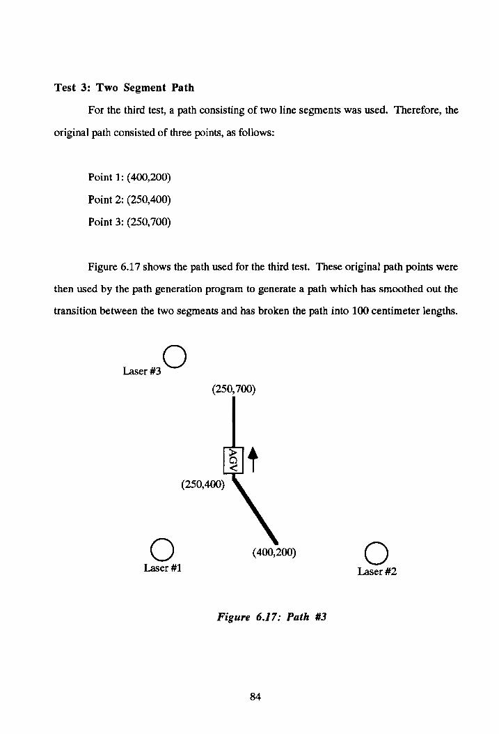
Test 3: Two Segment Path
For the third test, a path consisting of two line segments was used. Therefore, the
original path consisted of three points, as follows:
Point 1: (400,200)
Point 2: (250,400)
Point 3: (250,700)
Figure 6.17 shows the path used for the third test. These original path points were
then used by the path generation program to generate a path which has smoothed out the
transition between the two segments and has broken the path into 100 centimeter lengths.
Laser #3 o
(250,700)
o Laser #1
(400,200) o Laser #2
Figure 6.17: Path #3
84
Tests 3a, 3b, 3c:
Tests 3a, 3b, and 3c were run with the same parameters. They were:
Speed = 0.12 (Maximum = 1.00)
K (Smoothing Constant) = 1.0
Steering Activation Time = 0.4 seconds
Threshold Percentage = 50%
Path Segment Size = 100 centimeters
For this series of tests the results were good. There were no invalid position
updates during the runs. It was noticed that there is some lag inherent to the laser-based
positioning system during navigation. For example, when the vehicle was moving down
the X-axis and the X values of its position were decreasing, there was about a half-second
delay between when the vehicle got to a position and when the positioning system could
update its position to reflect that. When the vehicle was at x=250 centimeters, the system
would say it was at x=260 centimeters, which is where it was approximately one-half
second before. This causes the oscillation that was noticed earlier for testing of path #1.
This lag and the corresponding oscillation can be seen in Figure 6.18.
It is expected that the next generation laser-based positioning system from SPSi will
have less lag and should help to alleviate this problem. The absolute average path error for
tests 3a, 3b, and 3c was 11.8 centimeters, 20.7 centimeters, and 12.8 centimeters,
respectively. The poor results from test 3b were due to some erroneous position updates
from the system.
85

700
600
500
400
300
200
a
Tests 3d. 3e. 3f:
Recorded --......
Positioning system lag is evident here
100 200
....~----Path
300 Path3(x)
400
Figure 6.18: Results 0/ Test 3c
500 600
For these tests, the same parameters from tests 3a through 3c were used except that
the smoothing constant (K) was increased to 1.1 to try to eliminate some of the lag in the
system.
The results for these tests were good except that the system started giving invalid Y
position updates at the end of the path for tests 3e and 3f. In general, the results looked
86

very much like those of tests 3a through 3c, so the results will not be shown in graphical
form here. The absolute average path error for tests 3d, 3e and 3f was 12.4 centimeters,
10.9 centimeters, and 13.4 centimeters, respectively.
Tests 3~. 3h. 3i:
These tests were run with the same parameters as tests 3a through 3c, except the
smoothing constant (K) was reduced to 0.9. This was to see if the system reacted slower
than when K had a higher value.
In all three tests the positioning system returned some invalid values at one time or
another. For tests 3g and 3h, there were some points at the end of the path which were not
valid. During analysis, these points were removed from the data list to accurately reflect
how the system really behaved. Tests 3i had problems for almost the entire length of the
path. The positioning system was telling the navigation software that the vehicle was at
x=300 centimeters when the vehicle was actually at x=250 centimeters. Towards the end
of the path the positioning system did start returning valid values, however, and once again
the vehicle was able to attempt to get back on the desired path. In this case though, the
vehicle was almost at the end of the path by time it could recover, so the vehicle came to a
stop without getting very close to the path.
Figure 6.19 graphs the results of test 3g compared to the desired path. At the end
of the path some points are missing because the positioning system returned invalid data
and these points were deleted from the point list used to make the graph. In this test, the
system still appeared to have some lag, and reducing the value of K did not seem to have
any appreciable effect on navigation performance. For tests 3g and 3h, the absolute
average path error was 13.3 centimeters and 16.9 centimeters, respectively.
87

~ (f) .r::. as a..
700
600
500
400
300
200
o
Points were deleted at end of path
100
Tests 3j. 3k. 31:
200
...-..--- Path
300 Path3(x)
Recorded
400
Figure 6.19: Results of Test 3g
500 600
For these tests, it was decided to raise the value of the smoothing constant (K) to
1.2 to determine if the system would react better and perhaps eliminate some of the lag.
Figure 6.20 shows the results of test 31. Both test 3k and 31 went reasonably well,
although the system returned some invalid position updates near the end of test 3k.
However, these were not bad enough to seriously affect the navigation and the vehicle
88

continued after the positioning system recovered. Test 3j had problems during the whole
test but the vehicle managed to head towards the path at the end once the positioning system
recovered. The absolute average path error for tests 3k and 31 was 17.6 centimeters and
17.4 centimeters, respectively.
700
600
500
400
300
200
a 100
path/
200 300 Path3(x)
..... -- Recorded
400 500
Figure 6.20: Results of Test 31
89
600

Test 3m:
This was the last test run for Path #3. An attempt was made to use the same
parameters as for tests 3a through 3c, but with a speed of 0.20 and a smoothing constant of
1.1.
700
600
500 -.z, ('t) or. as a.
400
300
200
o
Points removed here -
Recorded
100 200 300 Path 3 (x)
400
Figure 6.21: Results of Test 3m
500
For this test, it can be seen that the system was basically underdamped and was
oscillating with a rather high amplitude. This is most likely due to the higher speed of the
vehicle which made it respond more to steering corrections. At the end of the path the
90
600
positioning system started returning invalid values. & before, these values were removed
in order to plot the graph. The absolute average path error for this test was 59.4
centimeters, which is deemed unacceptable for this system.
Further attempts were made to run the vehicle at a speed of 0.20 with a lower
smoothing constant (K) value. None of these tests were successful, however, and testing
was abandoned for these parameters.
Appendix D gives a complete, detailed listing of all parameters used for each test.
The reader should reference these for more details and notes about each test.
FURTHER DISCUSSION/PROBLEMS ENCOUNTERED
As mentioned earlier, there were a number of conditions under which testing was to
be conducted. The conditions involved the type of path to be navigated, the surface quality
and the velocity of the vehicle. It was desired to try have the vehicle navigate a closed-loop
path, such as a circle. This was attempted but due to lack of range and reliability of the
laser-based positioning system, the system was never able to complete a closed-loop path.
For this reason, the most complex path navigated was Path #2, which consisted of three
line segments.
It was also desired to have the vehicle run on different surfaces. Due to the limited
availability of the system, it was not possible to run the vehicle outside in a parking lot as
desired. All testing was confined indoors. The floor at the testing site was a smooth
concrete floor. There were no conduits or floor obstructions to test how well the vehicle
could navigate over a rough floor. It was decided to try to lay some extension cords on the
floor and have the vehicle run over them. However, since the system was ineffective at
speeds above one meter per second, the vehicle was not able to generate enough
momentum to drive over an extension cord without getting stuck. This is mostly a function
91
of the wheel and it would be interesting to try a future experiment with a vehicle with a
more robust drivetrain. It was also thought that navigation could be attempted with the
vehicle driving on an oil covered or contaminated surface. However, since the room was
in a new building, it was decided not to pour oil all over the new floor.
There were some additional testing problems and notes which are listed below.
Low Range of Positioning System
Although one of the strong points of the system is supposedly its extended range,
this system had a very low range of about ten meters. When the vehicle traveled further
than this the system was not reliable enough to consistently return positional data needed
for navigation. This was one of the reasons why closed-path navigation was not possible.
The next generation system should have better range of up to 250 meters, according to
SPSi.
Low Reliability Outside Region of Higher Accuracy
Chapter 3 (Methodology) described testing the system outside the triangle whose
vertices are formed by the three laser transmitters (see Figure 3.6). During testing, it was
noticed that the system was not giving any position updates outside this region. Upon
conferring with the SPSi engineer, it was noticed that the problem may lay with the
positioning system software. The system had been set-up for an earlier demonstration only
to return position updates within this triangle, in the interest of better reliability. The
engineer fixed this problem and the new software was used with the system. While this
solved the problem and allowed the positioning system to work outside this triangle, the
system was never reliable enough for navigation outside this triangle. This was also
probably a result of the limited range of the transmitters.
92

Blocking of Lasers From Receiver
Due to the design of the receiver located on the vehicle, the support armature
holding the reflector in place would periodically block an incoming laser signal. This was
not a problem when the vehicle was traveling in a straight line because the support armature
could be rotated away from the transmitters. However, when attempting to perform
closed-loop navigation, there will have to be some point where this armature will block an
incoming laser signal. This problem will be alleviated with the new system which does not
use any type of armature to support the reflector.
Extraneous Light Interference
During testing, it was noticed that the system ran the best and was most reliable at
night with minimal light on in the testing environment. Also, the system was more reliable
when the weather was overcast than when the sun was shining through the windows of the
testing room. In order to help reduce multipath interference from the windows, translucent
plastic sheeting was used to cover the windows. It is believed that this helped improve the
reliability of the system.
Overall System Reliability
In general, the largest problem faced was with the positioning system returning
valid position updates. The reasons for this are many, and some of them are outlined
above. It is hoped that the next generation system will be more reliable than the current
system.
DXF File Problem
It was noticed during testing that when a path was created using CANVAS software
on an Apple Macintosh, that the coordinates given in CANVAS were different from those
in the DXF file for the path. The shape of the path remained the same, but the coordinates
93
changed. It is not known whether this problem also occurs in other graphics software such
as AutoCAD. This problem required editing the DXF file before generating a path.
Delay of Positioning System
As one can see from the test results, the positioning system had some lag present.
It is, of course, impossible for any system to give instantaneous position updates, but it is
hoped that the next generation system will have less lag than the present system. This lag
generally caused the system to overshoot its target and to oscillate slightly when traveling in
a straight line.
94

Chapter 7 CONCLUSIONS
The purpose of this research was to determine the feasibility of a laser-based
positioning system as a primary navigation method. The system developed for this
research consisted of an automated guided vehicle which navigated solely with the use of
the laser-based positioning system in real-time. To date, there are no systems which can
navigate a pre-defined path using such a positioning system. Some lessons were learned
by the researcher, however, concerning the viability of this system in an industrial
environment. The system should have had the following advantages over previous
systems: 1) Greater range, 2) no prior structuring of environment, 3) real-time navigation,
and 4) no reliance on dead-reckoning for navigation.
The results showed that goals two through four had been met and are advantages of
this system over current systems. The range of this system is limited, however, but it is
believed that the next generation system should have greater range than the system used in
this research.
Since the goal of the research was to determine if the vehicle could use such a
system for navigation, various tests were carried out to determine how the system reacted
under certain conditions. Through the navigation software, the user could modify
parameters which would affect the performance" and accuracy of the vehicle as it traversed
its path. The goal of this research was not to determine which of these parameters were
critical success parameters to achieve the optimal navigation results. An area of future
research would be to examine these parameters and to determine how they affect
performance using modem statistical analysis techniques such as design of experiments. It
is possible that some of the parameters have little or no effect on the navigation of the
95

vehicle and could be held constant by the software. On the other hand, other parameters
could be extremely sensitive to the navigation results.
Overall, the research was successful. The best test result on the most complex path
(Path #2) resulted in an average path error of ±10 centimeters. This type of path was much
more indicative of the type of path one would use in encounter in an industrial
environment. This was over a distance of approximately six meters. On average, when the
positioning system was reliable enough to allow complete navigation of the path, the errors
tended to be anywhere from ±10 centimeters to ±20 centimeters. The maximum speed of
the vehicle with the system was about one meter per second.
The system performed much better on the straight line path, allowing higher vehicle
velocities with accuracy of approximately ±S centimeters. A straight line path is not usually
encountered in an industrial setting, however, so the straight line results only demonstrated
the basic navigational capabilities of the system. In general, the system ran better the
slower the vehicle traveled. One must take care though, to realize how reducing the speed
affects the navigation characteristics of the vehicle, particularly with regard to steering input
response.
It is also important to note that the vehicle's recorded path tended to be jagged and
not very smooth. This is a function of the multiple, rapid steering corrections made during
navigation. This is not really an issue when navigating around an industrial environment,
since the amplitude of these jagged deviations was no more than a few centimeters.
However, this would probably not make the system viable for such applications as painting
a pattern in a parking lot, for example. Future work could refine the navigation algorithm
to smooth out the response of the vehicle.
The system needs to be more reliable and robust before it could safely be used in an
industrial environment. Many of the problems encountered were due to the unreliability of
the laser-based positioning system. It should be noted that the system used was
96

approximately two years old, and was the first prototype positioning system manufactured
by Spatial Positioning Systems, Inc. It had been modified and used in many experiments
and was, for all intents and purposes, near the end of its useful life. It was discovered after
the experiment, that there was a focusing problem with laser transmitter number one, and
this most likely contributed to the range and reliability problems of the system as a whole.
Future testing should ensure that the system is capable of navigating a closed-looped path
repeatedly, as this was not tested during this research. Such a path would be very
indicative of the type of path one would encounter in industry.
In addition, some of the software used to determine position was not up to date and
this also contributed to the low reliability of the system. A new system is currently being
manufactured (as of June 1993) and should be ready for implementation during the summer
of 1993. This system will offer greater range and reliability and should be able to improve
the overall system performance significantly.
One point worth mentioning is that the accuracy of the system was very good. It is
not thought that the new system's path error will be any better than the old system when the
old system was operating correctly. The only area that may improve will be with respect to
the lag of the positioning system, which will be less with the new system, and may
therefore give better results. However, the reliability of the old system was only significant
in that it limited the number of successful tests. Many tests could not be completed because
the positioning system stopped generating valid data sometime during path traversal. With
the new system, it is thought that many more tests will be able to be run due to the
increased system reliability.
As mentioned earlier, some future development work will be necessary before this
system could be implemented in an industrial environment. Listed below are some possible
areas of improvement and future work which can be done on this system.
97

FUTURE AREAS OF RESEARCH
Heading Determination
For this research, the heading of the vehicle was determined by finding the direction
of a vector which connects the current vehicle position to the last recorded vehicle position.
This method was used because only one receiver was on the vehicle. The problem with
this is that this is only an approximation of the true heading of the vehicle. In most cases,
the vehicle has had some sort of steering correction between points and therefore will have
a different heading than is calculated.
A way to improve this would be to mount two receivers on the vehicle. The
heading could then be determined by finding the direction of a vector connecting the two
receivers. This would allow a much more accurate and timely heading indication than one
receiver would allow. Another advantage of two receivers would be error detection. When
a position update is received by both receivers, software could check to make sure that the
positions returned are located where they should be. For example, if the receivers are
located 30 centimeters apart on the vehicle, than the distance between the two position
updates received should be approximately 30 centimeters. If one of the receivers generated
a bad position update, this distance would probably not be near 30 centimeters and the
software could ignore the data and wait until valid data was received.
Minimum Update Distance
As mentioned in the results section, the software was modified to ignore position
updates until the vehicle traveled five centimeters. It would be interesting to change this
parameter and to see its effect on navigation. A good way to do this would be to include its
value on the main parameter menu of the navigation software, allowing the user to easily
change its value.
98

Error Recovery
During testing, there were numerous instances where the positioning system
stopped returning position updates. In these cases the vehicle simply continued moving
along in the direction it was going when it stopped receiving position uJXlates. A good idea
would be to add some intelligence to the navigation software when this happens. This
could involve keeping track of the time since the last position update, and slowing the
vehicle down as this time increases. Eventually, the vehicle could stop if enough time has
expired without receiving a position update.
Overall, the vehicle did a good job of getting back on course once the positioning
system recovered. There were, however, times when the positioning system did not
recover and the vehicle simply headed off in some random direction and needed to be shut
off with the emergency stop. In these cases it would have been better for the vehicle to
stop and wait for the system to recover. The system generally has more of a chance of
recovering if the vehicle is not moving than if the vehicle is in motion.
RegUlate Vehicle Velocity
For this research, the vehicle velocity was set by sending an integer between 127
and 255 to the driver motor controller. How fast the vehicle went for any speed value was
dependent on how loaded the vehicle was, the surface condition of the floor, obstructions,
and any inclination of the floor. A better way to control speed would be for the user to
enter a desired speed in meters per second and then to calculate the actual velocity by
dividing the distance traveled between two position updates by the time between those
updates. The velocity could then be monitored and raised or lowered as necessary. This
would allow the vehicle to travel at more consistent speeds regardless of the conditions at
the time.
99

Filtering of Invalid Data
Some sort of software filter could be used to filter out points which are obviously
out of range of where the vehicle could be. This could be done by determining the time
since the last position update and determining whether the vehicle was capable of traveling
the distance between the two positions in the given time frame. As mentioned earlier, this
problem can also be partly rectified by using two receivers on the vehicle. The two receiver
solution may not work however, ifboth receivers return invalid data.
Next Generation System
The next generation laser-based positioning system should be available from Spatial
Positioning Systems, Inc. by mid-summer 1993. It would be very much recommended to
use this new positioning system with the current navigation system on the vehicle. This
should allow greater range to perform closed-loop testing over a larger area.
Outdoor Navigation
As mentioned earlier, due to time and system availability constraints, the system
was never tested outside. This could be done with the new system to determine the
maximum effective range of the system. According the SPSi, the new system should have
a range of 250 meters.
Path Generation and Navigation Software
The Path Generation Software could be improved to take into account such things
as discontinuous paths, variable speeds, and forward and reverse vehicle travel, to name a
few. In addition, the user interfaces of both programs could be improved to provide more
error checking. Another future modification would be to convert the software to run under
the Windows operating system, allowing easier use than the existing DOS-based user
interface.
100
REFERENCES
AutoCAD Release 10 Reference Manual. (1989). (pp. 395-420). Autodesk, Inc.
Bevan, M. (1986). Free-Ranging Automatic Guided Vehicles Become Reality. In Hollier, R. H. (Ed.), Proceedings of an Executive Briefing: Automated Guided Vehicle Systems. (pp. 151-157). New York: Springer-Verlag.
Boegli, P. (1985). A Comparative Evaluation of AGV Navigation Techniques. In Proceedings of the 3rdInternationai Conference onAGVS. (pp. 169-180). Bedford (UK): IFS Publications.
Bennett, M. E., Miller, R. A., Stein, B. N. (1977). Plane Trigonometry. Philadelphia, Pennsylvania: W. B. Saunders Company.
Cox, I. J. (1991). Blanche - an Experiment in Guidance and Navigation of an Autonomous Robot Vehicle. IEEE Transactions on Robotics andAutomation, 7. (pp. 193-204).
Cox, I. J., Nelson, W. L. (1990). Local Path Control for an Autonomous Vehicle. In Autonomous Robot Vehicles. (pp. 38-44). New York: Springer-Verlag.
Evans, D. F. (1988). Lasers Liberate Guided Vehicles. Engineering(London), V. 228, No. 11. (pp. 610-611).
Forster, S. (1989). Mobile Autonomous Robot Performs Free-Ranging AGV Operation. In Proceedings of the 7th International Conference on AGVS. (pp. 57-68). Bedford (UK): IFS Publications.
Frohn, H., von Seelen, W. V. (1989). VISOCAR: An Autonomous Industrial Transport Vehicle Guided by Visual Navigation. In Proceedings of the 1989 IEEE International Conference on Robotics and Automation. (pp. 1155-1158). Washington, D.C.: IEEE Computing Society Press.
Gonzalez, J., Stentz, A., Ollero, A. (1992). An Iconic Position Estimator for a 2D Laser Range-Finder. In Proceedings of the 1992 IEEE International Conference on Robotics and Automation. (pp. 2646-2651). Washington, D.C.: IEEE Computing Society Press.
Hammond, G. C. (1986). Evolutionary AGVS - From Concept to Reality. In Hollier, R. H. (Ed.). Proceedings of an Executive Briefing: Automated Guided Vehicle Systems. (pp. 1 - 7). New York: Springer-Verlag.
Hammond, Gary. (1986). AGVS at Work. New York: IFS Publications.
Hollier, R. H. (Ed.). (1986). Proceedings of an Executive Briefing: Automated Guided Vehicle Systems. New York: Springer-Verlag.
Hollier, R. H. (Ed.). (1987). Automated Guided Vehicle Systems. New York: SpringerVerlag.
Hongo, T., Arakawa, H., Sugimoto, G, Tange, K., Yamamoto, Y. (1986). An Automatic Guidance System of a Self-Controlled Vehicle. In Cox, IJ., Wilfong, G. T. (Eds.), Autonomous Robot Vehicles. (pp. 32-37). New York: Springer-Verlag.
101

Horrocks, R. (1989). The Role of AGV Systems in Modem Assembly. In Proceedings of the 7th International Conference onAGVS. (pp.135-142). Bedford (UK): IFS Publications.
Jarvis, R. A., Byrne, J. C., Ajay, K. (1988). An Intelligent Autonomous Guided Vehicle: Localisation, Environmental Modelling and Collision-Free Path Finding. In Robots: Coming of Age. Proceedings of the International Symposium and Exposition on Robots. (pp. 767-781). New York: Springer-Verlag.
Jiinemanq, Prof. Dr.-Ing. Reinhardt. (1988). Integrierte Materialflupsysteme. Koln: Verlag TUV Rheinland GmbH.
Kopp, G. (1987). Wireless Guidance of AGVs. In Proceedings of the 5th International Conference onAGVS. (pp. 157-170). Bedford (UK): IFS Publications.
Le Corre, J. F., Garcia, G. (1992). Real-Time Determination of the Location and Speed of Mobile Robots Running on Non-Planar Surfaces. In Proceedings of the 1992 IEEE International Conference on Robotics andAutomation. (pp. 2594-2599). Washington, D.C.: IEEE Computing Society Press.
Lindgren, H. (1987). Centralised and Decentralised Control of AGVs. In Hollier, R. H. (Ed.). Automated Guided Vehicle Systems. (pp. 79-86). New York: SpringerVerlag.
McEllin, P. (1987). AGV Designs. In Hollier, R. H. (Ed.). Automated Guided Vehicle Systems. (pp. 53-63). New York: Springer-Verlag.
McGillem, C., Rappaport, T. S. (1988). Infra-Red Location System for Navigation of Autonomous Vehicles. In Proceedings of the 1988 IEEE International Conference on Robotics and Automation. (pp. 1236-1238). Washington, D.C.: IEEE Computing Society Press.
Mesaki, Y., Masuda, I. (1992). A New Mobile Robot Guidance System Using Optical Reflectors. In Proceedings of the 1992 IEEE/RSJ International Conference on IntelligentRobots and Systems. (pp. 628-635). New York, NY: IEEE.
Milller, T. (1987) AGVs in Europe - Current Techniques and Future Trends. In Hollier, R. H. (Ed.). Automated Guided Vehicle Systems. (pp. 11-17)New York: SpringerVerlag.
Nishide, K., Moritomo, H., Kondo, T. (1986). Automatic Position Findings of Vehicle by Means of Laser. In Proceedings of the 1986 IEEE International Conference on Robotics and Automation. (pp. 1343-1348). Washington, D.C.: IEEE Computing Society Press.
Piepel, U. (1989). Mobile Robots Based on AGV. In Proceedings of the 7th International Conference on AGVS. (pp. 13-24). Bedford (UK): IFS Publications.
Premi, S. K., Besant, C. B. (1983). A Review of Various Guidance Techniques That Can Be Used By Mobile Robots or AGVs. In Proceedings of the 2nd International Conference onAGVS. (pp. 195-210). Bedford (UK): IFS Publications.
Rathbone, R., Valley, R., Kindlmann, P. (1986). Beacon-Referenced Dead Reckoning: A Versatile Guidance System. Robotics Engineering, V. 8, No. 12. (pp. 11-16).
102

Spatial Positioning Systems, Inc. Executive Overview. (1992). Spatial Positioning Systems, Inc.: Blacksburg, Virginia.
Tsumura, T., Hashimoto, M. (1986). Positioning and Guidance of Ground Vehicle By Use of Laser and Comer Cube. In Proceedings of the 1986 IEEE International Conference on Robotics andAutomation. (pp. 1335-1342). Washington, D.C.: IEEE Computing Society Press.
Van Brussel, H., Van Helsdingen, C. C., Machiels, K. (1988). FROG - Free-Ranging on Grid: New Perspectives in Automated Transport. In Proceedings of the 6th International Conference on AGVS. (pp. 223-232). Bedford (UK): IPS Pub lica tions.
Wakaumi, H., Tsukagoshi, T., Miura, T., Yamauchi, F. (1988). A Magnetic Lattice Lane AGV System with Semi-Autonomous Movement. In Proceedings of the 6th International Conference onAGVS. (pp. 233-240). Bedford (UK): IPS Publications.
White, J. A., Pence, I. W. (Eds.). (1989). Progress in Materials Handling and Logistics. New York: Springer-Verlag.
Wiklund, U., Andersson, U., Hyyppa, K. (1988). AGV Navigation by Angle Measurements. In Proceedings of the 6th International Conference on AGVS. (pp. 199-212). Bedford (UK): IFS Publications.
Yates, B. D. (1988). Simple, Profitable Automatic Guided Vehicle Installations. In Proceedings of the Institution of Mechanical Engineers: Advanced Handling Systems -Applications and Experiences. (pp. 5-12). Suffolk (UK): Mechanical Engineering Publications.
103

APPENDIX A
SAMPLE DXF DATA FILE
104

0 7 22 SECTION 20 4.5
2 10 13 HEADER 9 0.0
9 $GRIDMODE 23 $ACADVER 70 0.0
1 1 14 ACI006 9 1.0
9 $GRIDUNIT 24 $AXISMODE 10 1.0
70 0.1250 15 0 20 0.0
9 0.1250 25 $AXISUNIT 9 0.0
10 $SNAPMODE 16 0.0625 70 0.0
20 1 26 0.0625 9 0.0
9 $SNAPUNIT 36 $CECOLOR 10 1.0
62 0.1250 17 7 20 0.0
9 0 27 $CELTYPE 9 0.0
6 $SNAPSTYLE 37 CONTINUOUS 70 0.0
9 0 40 $CLAYER 0 9.0
8 ENDSEC 41 Layer #1 0 2.891304
9 SECTION 42 $EXTMIN 2 50.0
10 TABLES 43 0 0 0.0
20 TABLE 44 0 2 0.0
30 VPORT 50 0 70 0.0
9 2 51 $ EXTMAX 0 0.0
10 VPORT 71 7 2 0
20 * ACTIVE 72 10 70 100
30 0 73 0 10 1
9 0.0 74 $LIMMIN 20 1
10 0.0 75 0 11 0
20 1.0 76 0 21 0
9 1.0 77 $LIMMAX 12 0
10 13.01087 78
105

0 1.0 1 0 50 70
ENDTAB 0.0 0 0 71 40
TABLE 0 0.0139 2 42 41
LTYPE 0.2 0.0139 70 3 0
1 txt VERTEX 0 4 8
LTYPE LAYERI 2 0 10
CONTINUOUS ENDTAB 2 70 0 20
64 TABLE 9 3 2 30
Descriptive Text VIEW 0 72 70 42
65 0 0 73 0 70
0 ENDTAB 0 40 0 0
0 TABLE VERTEX 0 2 8
ENDTAB UCS LAYER 1 0 70 10
TABLE 0 4 2 0 20
LAYER ENDTAB 9 70 0 30
1 TABLE 0 0 2 42
LAYER DWGMGR 0 2 70 70
LAYER 1 0 0 70 0 0
0 ENDTAB VERTEX 62 0 8
7 ENDSEC LAYERI 6 0 10
CONTINUOUS SECTION 3 0 2 20
ENDTAB BLOCKS 7 0 0 30
TABLE END SEC 0 2 0 42
STYLE SECTION 0 70 2 70
1 ENTITIES 0 0 0 0
STYLE POLYLINE VERTEX 2 8 8
STANDARD LAYER 1 LAYER 1 70 6 10
0 CONTINUOUS 2 40 62 20
0.0 7 9 41 66 30
106

o 42
o 70
o o
SEQEND o
ENDSEC o
EOF
107

APPENDIX B
PATH GENERATION SOFTWARE PROGRAM LISTING
108

PATHGEH.C Tue.day, June 1, 1993 4:44 PM
#include <stdio.h> #include <string.h> #include <math.h> #include "pathgen.h"
/****************************************************************/ /* */ /* Program: PathGen, {c)1993 Jeff Fithian */ /* Author: Jeff Fithian */ /* Version: 1.1 */ /* Date: March, 1993 */ /* Description: This program will be used to translate a */ /* DXF file to AGV path commands. The DXF file contains */ /* information describing a polyline which was drawn by */ /* the user in another program which can export graphic */ /* files in the DXF fonnat (i.e. Canvas, AutoCAD). The */ /* user can specify the speed of the AGV along the path */ /* and the program will create a text file which can be */ /* read by the AGV to follow the path drawn by the user. */ /* */ /****************************************************************/
/****************************************************************/ /* */ /* Function: Path_File_Init */ /* Description: This function will read get a file name fram */ /* the user and scan the current directory to determine if */ /* the file exists. The file name will be used later in */ / * the program to extract the points fram the DXF data * / /* */ /****************************************************************/ void Path_File_Init{char In_File[81]) {
}
int FILE
do {
err_flag=O; *Infile-ptr;
err _ flag=O ; if «Infile-ptr=fopen{In_File, "r") )=NULL) /* OPEN FILE */
{ printf{"\nCan't OPEN file: %s\n", In_File); err_flag = 1; }
} while (err_flag); printf("\nFile %s was opened successfully.\n",In_File); fclose(Infile-ptr);
/****************************************************************/ /* */ /* Function: Calc Path */
109
Page 1

PATBGBR.C Page 2 Tuesday, June 1, 1993 " : "" PM
/* Description: This function will calculate the path which */ /* AGV must follow. The path will be described as a */ /* series of points along the path separated by an */ /* interval described by STEPSIZE. */ /* */ /****************************************************************/
void Calc_Path(int *index, Vect vector[NUM_PTS-l], Ppoint path[PATHSIZE], Ppoint points [NUM_PTS] , float *StepSize, char OUt_File[Sl])
{ Ppoint segpoints[200]; /* untransformed path points for the
int nmnsteps,
vecnum, segnum,
p=O ,k, j, dir;
current vector */ /* number of path points on the
current vector */ /* current vector number */ /* path point counter for the
current vector */ /* counters */ /* direction of arc, up or down */
Ppoint delta; /* starting x,y coordinate of current
float
FILE double
arctheta, theta, i, thisy, nexty; *fptr; *ptr;
vector */ /* delta theta for arc segments */ / * current angle to calc arc * / / * xcoord of points on linear vector * / / * untransformed y coord of current vector * / /* untransformed y coord of next vector */
for (vecnumFO;vecnum<=(*index-2);vecnum++) {. k=O; / * save the starting point of the current vector to be
used to transfonn the points to path coordinates */ delta.x=points[vecnum].x; delta.y=points[vecnum].y;
/* Calculate the untransformed path points along the linear part of the vector * /
for (i=vector[vecnum].startptii<=vector[vecnum].endpt; i+=*stepSize) { segpoints[k].x=ii segpoints [k] • y=O ; k+=l; /* printf(" x=%4.1f y=%4.1f\n",i,O); */ }
if (vecnuml=(*index-2» /* do not calculate arc if it is the last vector */
{ /* Calculate the untransformed path points along the
110

PATHGZH.C Page 3 Tue.day, June 1, 1993 4: 44 PM
arc which is used to join to linear vectors. The first step is to compute the angle interval to be used to calculate the path points around the arc */ arctheta=fabs(2*asin(*StepSize/2/vector[vecnum].roc»:
/* Use this angle increment to calculate the points around the arc * / /* determine whether arc goes above or below vector */
thisy=points[vecnum+l].x*sin(-vector[vecnum].theta) +points[vecnum+l].y*cos(-vector[vecnum).theta);
nexty=points[vecnum+2].x*sin(-vector[vecnum].theta) +points[vecnum+2].y*cos(-vector[vecnum].theta):
if (thisy<nexty) dir=UP;
else dir=oc::MN ;
for (theta=PI/2-arctheta:theta>=(-PI/2+vector[vecnum].thetal): theta-=arctheta)
{ segpoints[k].x=vector[vecnum].endpt +
vector[vecnum].roc*cos(theta); segpoints[k].y=dir*vector[vecnum].roc +
-dir*vector[vecnum).roc*sin(theta); k+=l; }
} k-=l:
/ * Transform the path points from the vector coordinate system to the path coordinate system */
for (j=O;j<=k;j++)
}
( path[p].x=segpoints[j].x*cos(vector[vecnum].theta)
-segpoints[j].y*sin(vector[vecnum].theta) +delta. x;
path[p].y=segpoints[j].x*sin(vector[vecnum].theta) +segpoints[j].y*cos(vector[vecnum].theta} +delta·Yi
p+=l: / * increase path counter * / }
/ * Set last point on path to be last point of polyline * / path[p].x=points[*index-l].x; path[p].y=points[*index-l].y;
printf ("number of points in path=%d\n", p) ; /* Save data in output file */ printf( "Saving data in %s" ,OUt_File}; fptr==fopen (Out _F ile, "w" ) ; fprintf(fptr, "%d\nlt ,p); for (j=O;j<=p;j++) {
fprintf{fptr, "%6.3f %6.3f\n" ,path[j] .x,path[j] .y);
111

PATHQZN.C Page .. Tu •• day, June 1, 1993 4:44 PM
} fclose ( fptr) :
}
/****************************************************************/ /* */ /* Function: Calc_Vector_Dims */ /* Description: This function will calculate the magnitude */ /* and direction of the straight line segments which make */ /* up the desired travel path for the AGV. These vectors */ /* do not include the curved segments computed at */ /* intersections of path segments. They will be * / /* calculated later. */ /* */ /****************************************************************/ void Calc_Vector_Dims(Ppoint points [NUM_PTS] , int *index,
{ int Ppoint float
Vect vector[NUM_PTS-l], float *Xmult, float *Ymult, float *Rc:x::mult)
i; delta: r, /* radius of curvature b/w two vectors */ d, /* distance to intersection of curve and vector */ cmag; /* magnitude of */
printf( "'d points read:\n" ,*index): /* scale points */ for (i=O;i<=(*index-l):i++)
{ points [ i] • x=points [ i] • x* ( *XDlul t) ; points [ i] • y=points [i] • y* ( *Ymul t) : }
for (i=O;i«*index-l);i++) {
/* Calculate magnitUde of vector */ delta.x=points[i+l].x-points[i].x; delta.y=points[i+l].y-points[i]·Yi /* set x and y components of vector */ vector[i].x=delta.x; vector[i].y=delta.y: vector[i].d=sqrt(delta.x*delta.x + delta.y*delta.y);
/* Determine direction of vector from 0 to 2_ */ /* Is vector in first or fourth quadrant? * / if (delta.x>O)
vector[i].theta=atan(delta.y/delta.x); else / * Is vector in second or third quadrant? * /
if «delta.x<O) && (delta.yJ=O» if (delta.y<O) /* 3rd quadrant */
112
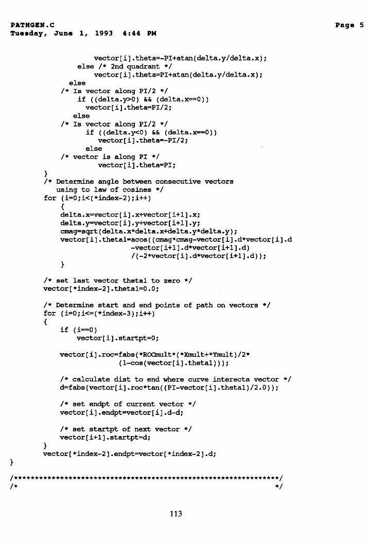
PA~HGBH.C Page 5 ~u.e.day , Ju.ne 1, 1993 , :,' PM
}
}
vector[i].theta=-PI+atan(delta.y/delta.x}; else / * 2nd quadrant * /
vector[i].theta=PI+atan(delta.y/delta.x}; else
/* Is vector along PI/2 */ if «delta.y>O) && (delta.x==O»
vector[i].theta=PI/2; else
/* Is vector along PI/2 */ if «delta.y<O) && (delta.x==O»
vector[i].theta=-PI/2; else
/* vector is along PI */ vector(i].theta=PI;
/* Determine angle between consecutive vectors using to law of cosines * /
for (i=O;i«*index-2};i++) { delta.x=vector[i].x+vector[i+l].x; delta.y=vector[i].y+vector[i+l].y; cmag=sqrt(delta.x*delta.x+delta.y*delta.y); vector[i].thetal=acos«cmag*cmag-vector[i].d*vector[i].d
}
-vector[i+l].d*vector[i+l].d) /(-2*vector(i].d*Vector[i+l].d»;
/* set last vector thetal to zero */ vector[*index-2].thetal=O.O;
/* Determine start and end points of path on vectors *1 for (i=O;i<=(*index-3);i++) {
}
if (i~O) vector[i].startpt=O;
vector[i].roc=fabs(*ROCmult*(*Xmult+*Ymult)/2* (l-cos(vector[i].thetal»);
1* calculate dist to end where curve interects vector *1 d=fabs(vector[i].roc*tan«(PI-vector[i].thetal)/2.0»;
1* set endpt of current vector */ vector[i].endpt=vector[i].d-d;
/* set startpt of next vector *1 vector[i+l].startpt=d;
vector[*index-2].endpt=vector[*index-2].d;
1****************************************************************1 /* *1
113

PATHQEII.C Tue.day, June 1, 1993 4:44 PM
/* Function: Read_Path_File */ /* Description: This function will read the DXF data file */ /* passed in the file_name variable and extract the points */ /* of the polyline vertices. The x,y coordinates for the */ /* points will be stored in the points structure. The */ / * number of points read will be stored in the index var. * / /* and sent back to the calling function. */ /* */ /****************************************************************/ void Read_Path_File(char In_File[S1], Ppoint points [NUM_PTS] , int *index,
Vect vector[NUM_PTS-l],float *Xmult, float *Ymult,
{
}
int char FILE float
float *ROCmult)
i; vertex [ ] = "VERTEX" , input_line [ SO ] ; *fileytr; Z;
fileytr=fopen(In_File, "r"); while ( fgets(input_line,SO,fileJltr) 1= NULL)
{ if (strncmp ( input_line, vertex, 6 ) ==0 ) {
}
for (i=1;i<=3;i++) fgets(input_line,SO,fileJltr); fscanf(fileJltr, "%f" ,&points[*index] .x); fgets(input_line,SO,fileJltr); fgets(input_line,SO,fileytr); fscanf(fileytr, "%f" ,&points[*index] .y); fgets(input_line,SO,fileytr); fgets(input_line,SO,fileytr); fscanf(fileytr,"%f",&z); *index+=l;
} fclose(fileytr); if (*index-O) ERR FLAG--TRUE: if (IERR FLAG) -
Calc_Vector_Dims(points,index,vector,Xmult,Ymult,ROCmult);
/****************************************************************/ /* */ /* Function: Change_Path_Params */ /* Description: This function will allow the user to change */ /* any of the parameters used by this program to * / /* generate the path * / /* */ /****************************************************************/ void Change_Path_Params(char In_File[Sl],char OUt_File[Sl],float *Xmult,
float *Ymult,float *StepSize,float *ROCmult)
114
Page 6

PATHGBN.C Tuesday, June 1, 1993 4 :44 PM
{ int Param;
printf ( "PARAMETERS: \n-----------\n" ) : printf("l) Input File: %s\n",In_File): printf("2) output File: %s\n",OUt_File); printf (" 3) X Scaling Factor: %f\n II , *Xmult) ; printf("4) Y Scaling Factor: %f\n",*Ymult); printf("S) Path Segment/Step Size: %f\n",*StepSize): printf{"6) Radius of Curvature Multiplier: %f\n",*ROCmult); printf( "7) Return to Main Menu\n"); printf("Enter Selection \(1 - 7\):"); scanf( !I%d" ,&Param); getchar{) ; switch (Param) {
case 1: printf( "Enter new input file n!Ulle: "); gets{In_File); break;
case 2: printf("Enter new output file name: "); gets (OUt_File) ; break;
case 3: printf("Enter new X scaling factor: "); scanf{ n%f" ,Xmult); getchar() ; break;
case 4: printf("Enter new Y scaling factor: "); scanf( "%f", Yrmllt); getchar() ; break;
case 5: printf ("Enter new segment step size: "); scanf ( "% f" , StepSize ) : getchar() ; break;
case 6: printf(ltEnter new ROC multiplier: "); scanf( "if" ,ROCmult): getchar() ; break;
} /* End switch statement */ } / * End Change Jarams function * /
/****************************************************************/ /* */ /* Function: Main_Path_Menu */ /* Description: This function will generate the main menu for */
115
Page 7
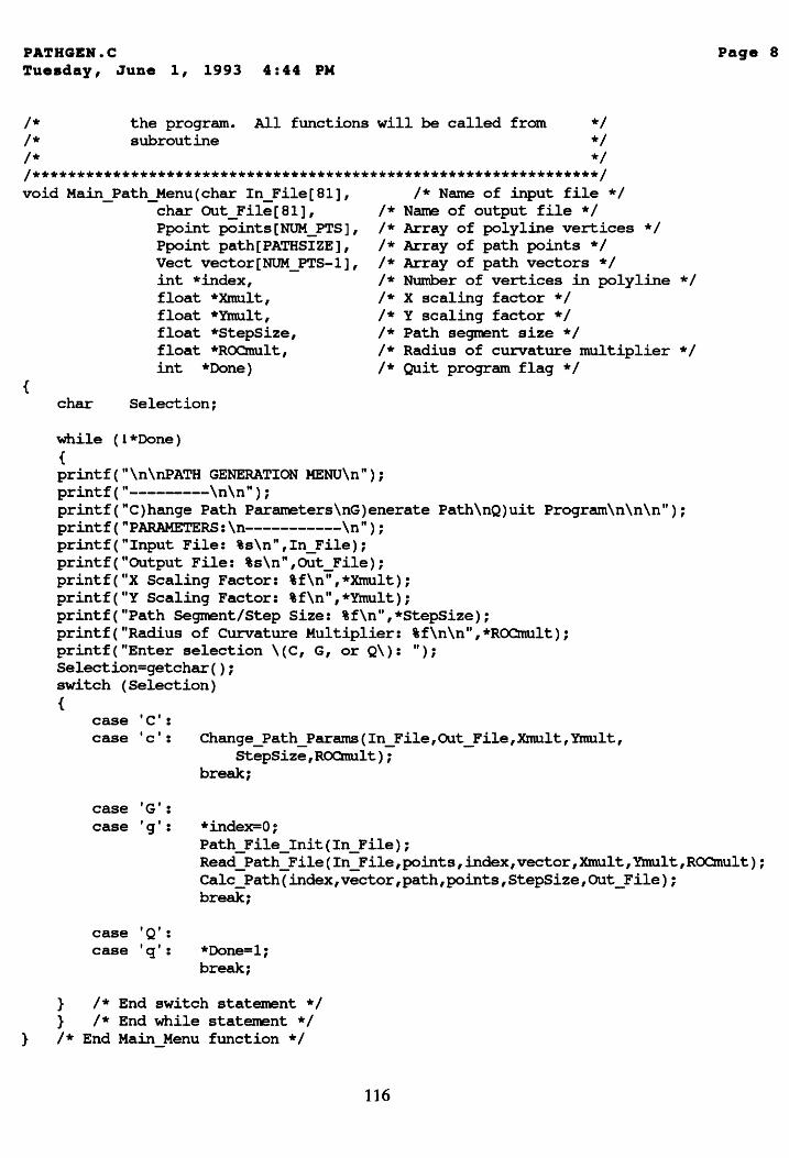
PATHGB:H.C Tue.day, June 1, 1993 4:44 PM
/* /* /*
the program. All functions will be called from subroutine
*/ */ */
/****************************************************************/ void Main_Path_Menu(char In_File[S!], /* Name of input file */
{
char out File[Sl], /* Name of output file */ Ppoint ~ints[NUM PTS], /* Array of polyline vertices */ Ppoint path[PATHSIZE], /* Array of path points */ Vect vector[NUM_PTS-l], /* Array of path vectors */ int *index, /* Number of vertices in polyline */ float *Xmult, /* X scaling factor */ float *Ymult, /* Y scaling factor */ float *stepSize, /* Path segment size */ float *ROCmult, /* Radius of curvature multiplier */ int *Done) /* Quit program flag */
char Selection;
while (1 *Oone ) { printf ( If \n \nPATH GENERATION HENU\ntl); printf("---------\n\n"); printf("C)hange Path Parameters\nG)enerate Path\nQ)uit Program\n\n\ntl); printf ( "PARAMETERS: \n-----------\n " ) ; printf("Input File: %s\n",In_File); printf(nOUtput File: %s\nlt,OUt_File); printf("X Scaling Factor: %f\n",*Xmult); printf(lfy Scaling Factor: %f\ntl,*Ymult); printf("Path Segment/Step Size: %f\n",*Stepsize); printf("Radius of curvature Multiplier: %f\n\n",*ROCmult); printf("Enter selection \(e, G, or Q\): "); Selection=getchar(): switch (Selection) {
case 'C': case 'c':
case 'G': case 'g':
Change_Path_Params(In_File,out_File,Xmult,Ymult, StepSize,ROCmult);
break;
*index=O;
Page 8
Path_File_InitCIn_File); Read_Path_File(In_File,points,index,vector,Xmult,Ymult,ROCmult); Calc_Path(index,vector,path,points,StepSize,OUt_File);
case 'Q': case 'q':
break;
*Oone=!; break;
} /* End switch statement */ } /* End while statement */
} /* End Main_Menu function */
116

PATHGEH.C Tue.day, June 1, 1993 4:44 PM
/****************************************************************/ /* */ /* Function: Read_Path_Prefs */ /* Description: This function will read the default settings */ /* from the "path.prf" preferences file. */ /* */ /****************************************************************/ void Read Path Prefs(float *Xmnlt,float *Ymult,
float *Stepsize,char In_File[S!],char OUt_FilerS!], float *ROCmult)
{
}
FILE *fptr;
if ( (fptr=fopen(ttpath.prf","r"» 1= NULL) fscanf(fptr,tI%f %f %f %s %s %ftl,Xmnlt,Ymult,
StepSize,In_File, OUt_File, ROCmult)i fclose ( fptr) i
/****************************************************************/ /* */ /* Function: Write_Prefs */ /* Description: This function will write the default settings */ /* to the "path.prf" preferences file. */ /* */ /****************************************************************/ void Write_Path_Prefs(float *Xmnlt,float *Ymult,
{
}
float *StepSize,char In_File[Sl],char OUt_File[Sl], float *ROCmult)
FILE *fptr;
fptr=fopen( "path. prf tt , "w"); fprintf(fptr,tI%f %f %f %s %s %f",*Xmult,*Ymult,
*StepSize,In_File, OUt_File, *ROCmult)i fclose(fptr);
/************************************************************************/ /* */ / * This is the main program segment of the code. After * / /* file and AGV initialization is performed, control of the */ /* program is passed to the main menu function */ /* */ /************************************************************************/ void main(void) {
/* variables to be used by the path generation module of the program */
117
Page 9

PATHGBH.C Page 10 Tuesday, June 1, 1993 ,:,' PM
}
char
float
Ppoint
Vect int
int
In File[81]="AGV6.dxf", /* Input file name */ out File[81]="Pathtbl.dat"; /* output file name */ Xmult=lO, /* X axis scaling factor */ Ymult=10, /* Y axis scaling factor */ Speed=.5, /* Velocity of AGV in rn/s*/ MaxSpeed=l, /* Max velocity of AGV in rn/s*/ StepSize=.4, /* Path segment length */ Rocmult=.l; /* radius of curvature multiplier */ points[NUM_PTS], /* vertices */ path[PATHSIZE]j /* path of AGV in ref pt segments */ vector[NUM_PTS-l]j /* segment vectors */ index=O, /* number of vertices in drawing */ i, /* counter */ Done=O;
Main_Done=O, /* Main program exit flag */ Selection;
/* Read preferences file for path generation module parameters */ Read_Path_Prefs(&Xmult,&Y.mult,&StepSize,In_File,OUt_File,
&ROCmult) j
Main_Path_Menu(In_File,OUt_File,points,path, vector,&index,&Xmult,&Y.mult,&StepSize, &ROCmult,&Done);
/* write path generation module preferences to disk */ Write_Path_Prefs(&Xmult,&Ymult,&StepSize,In_File,OUt_File,
&ROCmult) ;
118

PATHGBH.H Page 1 Tue.day, June 1, 1993 4:47 PM
/* define constants #define NOM PTS #define PI -#define TRUE #define FALSE #define PATHSIZE #define MIN_SEG_DIST
for path generation module */ 100 /* max number of vertices */ 3.1415927 /* value of */ 1 o 500 1
/* number of points on a path */ /* minimum segment length. This will determine radius of curvature for cart. The higher this number, the larger the radius of curvature */
#define DatlN -1 #define UP 1
/ * define structures to be used * / struct coord / * structure for a point * /
{ float x; float y; };
typedef struct coord Ppoint; / * define Ppoint variable type * /
struct vectors / * structure to hold vector info * / { float d; /* magnitude */ float theta; /* direction */ float x; /* x value */ float y; /* y value */ float theta1; /* angle between it and next vector */ float startpt; /* point on vect where path starts */ float endpt; / * point on vect where path ends * / float roc; / * roc of arc to blend with next vector };
typedef struct vectors Vect; /* define Vect variable type */
int ERR FIAG=FALSE· - , /* Function Prototypes */ void Path_File_Init(char In_File[Sl]); void Calc_Path(int *index, Vect vector[NUM_PTS-1],
Ppoint path(PATHSIZE], Ppoint points [NUM_PTS] , float *StepSize, char out File[S1]);
void Calc_Vector_Dims(Ppoint points [NUM_PTS] , int *index, Vect vector[NUM_PTS-1], float *Xmult, float *Ymult, float *ROCmult);
*/
void Read_Path_File(char In_File[S1], Ppoint points[NUM_PTS], int *index, Vect vector[NUM_PTS-1],float *Xmult, float *Ymult, float *ROCmult);
void Change_Path_Params(char In_File[Sl],char OUt_File[81],float *Xmult, float *Ymult,float *StepSize,float *ROCmult);
void Main_Path_Menu(char In_File[81],char OUt_File[81], Ppoint points[NOM_PTS], Ppoint path[PATBSIZE],Vect vector[NUM_PTS-1],int * index, float *Xmult,float *Ymult,float *Speed,float *ROCmult,
119

PATHGSK.H Page 2 Tue.day, June 1, 1993 4:47 PM
int *Done); void Read_Path_Prefs(float *Xmult,float *Ymult,
float *StepSize,char In_File[81],char OUt_File[81], float *ROCmult);
void Write_Path_Prefs(float *Xmult,float *Y.mult, float *StepSize,char In_File[81],char OUt_File[81], float *ROCmult);
120

APPENDIX C
NAVIGATION SOFrWARE PROGRAM LISTING
121

RAVIBM.C !rue.day, June 1, 1993 4: 46 PM
#include <stdio.h> #include <string.h> #include <math.h> #include <bios.h> #include <conio.h> #include <stdlib.h> #include <dos.h> #include <time.h> #include "spsi.h" #include "intern.h" #include "extern.h" #include "int.h tl
#include !lser.h tl
#include "int. c" #include "ser.c" #include "nav.h" #include "nei.c"
#define SPEED 150 #define CENTER 132
FILE char
*sim_fptr; /* pointer to simulation event record file */ Event_File[81J="eventdat.dat"; /* File name for event record file */
/************************************************************************/ /* /* Program: Navigate, {c)1993 Jeff Fithian /* Author: Jeff Fithian /* Version: 1.1 /* Date: March, 1993 /* Description: This program will be used to navigate the /* AGV around a user defined path. The user must have /* already defined the path using a DXF file format and /* used the PathGen software to generate the path points. /* This path must be stored in a data file specified by /* the user. /*
*/ */ */ */ */ */ */ */ */ */ */ */
/************************************************************************/
/****************************************************************/ /* */ /* Function: Main_Nav_Menu */ /* Description: This function will generate the main menu for */ /* the program. All functions will be called from * / /* subroutine */ /* */ /****************************************************************/ void Main_NavJ(enu(
float *Update t, /* Simulation Update Rate */
122
Page 1

IfAVIBM.C Tue.day, June 1, 1993 4: 46 PM
{
float *Speed, /* Desired AGV speed * / float *MaxSpeed, / * Max AGV speed * / float *K, /* Angle smoothing coefficent */ float *deltat, /* time to steer AGV */ float *thresh, /* threshold percentage */ char In_File[81], /* Input file name */ char Pos _F ile [ 81 ] , /* Position record file name */ char ErrJile[ 81]) /* Error record file name */
char Selection; unsigned AGV_Speed; /* AGV Speed value (128-255) int Done=O;
while (1 Done) {
/* Quit program flag */
AGV _ Speed= 12 8 + (*Speed/ ( *MaxSpeed» * 127; printf( "\n\nNAVIGATION MENU\nlt); printf("---------\n\nlt); printf( "C)hange Parameters\nB)egin Navigation\n lt ); printf("S)i.mulate Navigation\nQ)uit Program\n\n\n"); printf ( "PARAMETERS: \n-----------\n II ) ;
printf("Input File: %s\n",In_File); printf( "AGV Speed: %f\n" ,*Speed); printf( "Maximum AGV Speed %f\n" ,*MaxSpeed); pr intf ( "SIooothing Constant: % f\n II , *K) ; printf( "Max Steering Activation Time: %f\n", *deltat); printf("Theshold Percentage: %f%\n",*thresh*100); printf( "Simulation Update Rate (sees): %f\n" ,*Update_t); printf("Position Record File Name: %s\n",Pos_File); printf("Error Record File Name: %s\n",Err_File); printf("Enter selection \(C, B, S, or Q\): tI); Selection=getchar(); switch (Selection)
{
*/
case 'c': case 'c': Change_Nav_Params(Update_t, Speed, MaxSpeed, K, deltat,
thresh,In_File,&AGV_Speed,Pos_File,Err_File); break;
case 'B': case 'b':
case'S' : case's' :
case 'Q': case 'q':
Init_AGV() ; Navigate_Path (K,deltat, thresh, In_File, &AGV_Speed,Pos_File,Err_File); break;
Init AGV(); Navigate_Sim(Update_t,K,deltat,thresh,In_File, &AGV_Speed,Pos_File,Err_File); break;
Done=l: break;
123
Page 2

HAVIBM.C Tue.day, June 1, 1993 4:46 PM
} /* End switch statement */ } /* End while statement */
} /* End Main_Nav Menu function */
/****************************************************************/ /* */ /* Function: Update_Pos */ /* Description: This function update the position of the AGV */ /* fram the laser based positioning system. The system */ 1* will return the X and Y coordinates of the vehicle. */ 1* */ /****************************************************************/ int Update_Pos(location *agv) {
}
if (position.head 1= position. tail) {
disable_int() : agv->x=( (float) position.pos[position.tail].x): agv->y=( (float) position.pos[position.tail].y):
1* printf( "x=%f y=%f\n" ,agv->x,agv->y): */
} else
position. tail = (position. tail < NUM_POS_IN_BUFF-l) ? position. tail + 1 : 0:
enable _ int ( ) : return (TRUE ):
return(FALSE) :
/****************************************************************/ /* */ /* Function: Update_Man_Pos */ /* Description: This function update the position of the AGV */ /* fram the user for testing purposes. */ /* */ /****************************************************************/ int Update_Man_Pos(location *agv) {
}
printf ("Enter the x coord: "): scanf ("%f" ,&agv->x): printf ("Enter the y coord: "): scanf( "%ftl ,&agv->y): return(TRUE):
1****************************************************************/ 1* */ 1* Function: calc_Angle */ /* Description: This function will calculate the angle of a */ 1* vector which connects the position of the AGV to the */ / * next point on the path. * /
124
Page 3
HAVIBM.C Tue.day, June 1, 1993 4: 46 PM
/* */ /****************************************************************/ float Calc_Angle(location *aqv,location *pt) {
}
float angle, / * angle between the two points * / deltax, /* delta x bet-ween the points */ deltay; /* delta y bet-ween the points */
deltax=pt->x - aqv->x; deltay=pt->y - agv->y:
/* Determine direction of vector fram 0 to 2 */ /* Is vector in first or fourth quadrant? */if (deltax>O)
angle=atan(deltay/deltax); else
/ * Is vector in second or third quadrant? * / if «deltax<O) " (deltayl=O)}
if (deltay<O) /* 3rd quadrant */ angle--PI+atan{deltay/deltax):
else / * 2nd quadrant * / angle-PI+atan(deltay/deltax):
else /* Is vector along PI/2 */
if «deltay>O) " (deltax==O» angle=PI/2 ;
else /* Is vector along -PI/2 */
if «deltay<O) && (deltax==O» angle=-PI/2;
else /* vector is along PI */
angle=PI; return(angle) ;
/****************************************************************/ /* */ /* Function: Correct AGV */ /* Description: This function will correct the path error of */ /* the AGV by turning the AGV wheel alpha degrees for */ /* deltat seconds. */ /* */ /****************************************************************/ void Correct_AGV(float *alpha, float *deltat, unsigned *AGV_Speed) {
unsigned AGV_angle; /* AGV angle value */
/* set speed */ io_agv-POinter->speed_dac=*AGV_Speed: set_speed() ;
125
Page 4

RAVIBM.C Tue.day, June 1, 1993 4: 46 PM
/* Set the AGV angle value */ AGV_angle= CENTER + -(*alpha)/1.5707963 * (255 - CENTER); io_agv-POinter->angle_dac=AGV_angle; printf( "AGV ANGLE=%d\n" ,AGV_angle); set_angle();
/* delay for specified time interval */ delay(*deltat*lOOO);
/* return front wheel angle to forward */ io_agv-POinter->angle_dac=CENTER; set_angle ( );
Page 5
fprintf (sim_fptr,"Turn AGV %f degrees for %f seconds ••• \n" , *alpha*180/PI, *deltat) ; printf("Turn AGV %f degrees for %f seconds ••• \n",*alpha*180/PI,*deltat);
}
/****************************************************************************/ /* */ / * Function: Navigate _ Sim * / /* Description: This function will be the main function used */ /* to simulate AGV navigaation around the path specified by */ /* the points in the path data file */ /* */ /****************************************************************************/ void Navigate_Sim(float *Update_t, float *K, float *deltat, float *thresh,
{ int
location
float
char In_File[Sl] ,unsigned *AGV_Speed, char Pos_File[Sl], char Err_File[Sl)
n, /* number of points in path */ dmrmy I / * durrmy point counter * / i, / * path point counter * / intphi, /* integer value of heading error */ DONE=O, /* Finish path flag */ new-POs=FALSE; /* flag to see if new pos was read */ agv, / * AGV location and heading * / prev_agv, /* previous AGV location and heading */ path..,pt, / * coordinates of path point * / last-pt; /* previous point on path */ deltaphi, /* heading error b/w agv and path */ phi2, /* angle b/w agv pos and next point on path */ alpha, /* steering angle to correct path */ theta, /* angle of current vector b/w last and current pt */ d, /* distance b/w two consecutive path points */ deltax, /* delta x b/w current and last path point */ deltay, /* delta y b/w current and last path point */ xdist, / * distance AGV has travelled b/w two points * / act_time, /* time to activate steering */ x, y, / * distance in x and y of agv from last point * / xerr , yerr, / * x and y random error * / v, / * AGV speed in em per second * /
126

HAVIBM.C Tue.day, June 1, 1993 4:46 PM
FILE
randomize ( ) ;
err, sum_err=O, ave_err, num_err=O, travel_d; *fptr, *pos_fptr, *err_fptr;
I * perpendicular distance from agv to path *1 1* sum of errors *1 1* average path error *1 1* number of error measurements taken *1 1* distance AGV travels in Update_t seconds *1 1* pointer to input file *1 1* pointer to position record file *1 1* pointer to error record file *1
1* Open error record file *1 err_fptr=fopen(Err_File, "w") ;
1* Open simulation event record file *1 sim_fptr=fopen(Event_File, "wit) ;
1* Open position record file *1 pos_fptr=fopen(Pos_File, "wit);
I * set agv to desired speed * I io_agv-POinter->speed_dac-*AGV_Speed; set_speed() ; v=(*AGV_Speed - 128) * 1.755; 1* AGV veloc. in em per second *1
fptr=fopen(In_File, "r"); fscanf(fptr,"%d",&n); fscanf(fptr,"%f %f",&last-pt.x,&last-pt.y); 1* read first point *1 fprintf(sim_fptr, "Read path point: x=%f y=%f\n" , last-pt.x,last-pt.y) ; fscanf(fptr,"%f %f",&path-pt.x,&path-pt.y); 1* read next point *1 fprintf(sim_fptr, "Read path point: x=%f y=%f\n" ,path-pt.x,path-pt.y) i
1* calculate distance from last point to present point *1 deltax=path-pt.x-last-pt.x; deltay=path-pt.y-last-pt·Yi d=sqrt(deltax*deltax + deltay*deltay);
1* determine angle of vector between last and current point *1 theta-Calc_Angle(&last-pt,&path-pt):
1* Set initial AGV position and heading to start of path *1 prev_agv.x=last-pt.x; prev_agv.y=last-pt·Yi agv.dir=theta; fprintf(pos_fptr,"%f %f\n",prev_agv.x,prev_agv.y);
i-2; act time=*deltat· - ,
Page 6
while (i<=n && 100NE) 1* execute until all points in path file have been read ." {
1* Calculate new AGV position *1 travel_d= act_time*v; 1* how many em did AGV travel? *1
127

HAVIBM.C Page 7 Tue.day, June 1, 1993 4:46 PM
agv.x=prev_agv.x + travel_d * cos(agv.dir); agv.y=prev_agv.y + travel_d * sin(agv.dir);
/* Add error to position of AGV */ xerr=«float) randam(200)-100.0)/SO; yerr=({float) randam(200)-100.0)/SO; agv.x=agv.x + xerr; agv. y=agv • y + yerr; fprintf(pos_fptr,"%f %f\n",agv.x,agv.y);
/* determine heading of AGV */ agv.dir=Calc~gle(&prev_agv,&agv);
fprintf(sim_fptr, uAGV position:x=%f y=%f dir=%f\n" ,agv.x,agv.y, agv.dir*1S0/3.1415);
printf("x=%f y=%f theta=%f\n",agv.x,agv.y,aqv.dir*1S0/3.1415);
1* transform AGV position to determine if it has passed point */ x=agv.x-last-pt.x; y=agv.y-last-pt.y; xdist=x*cos(-theta}-y*sin(-theta);
/* Calculate error in AGV position defined as perpendicular distance fram AGV to path * /
err=fabs(x*sin(-theta)+y*cos(-theta»; nlD'n_err+=1; slD'n_err=sum_err + err; £printf(err_fptr, "%f\n" ,err);
if (i=n && xdist>=d) DONE=1; while (xdist>=*thresh*d && il=n) /* read new path point if AGV is ready to */
{ 1* Save previous points */ last-pt.x=path-pt.x; last-pt.y=path-pt.y; / * Read new point fram file * / fscan£(fptr, U%f %f" , &path-pt.x,&path-pt.y) ; /* get next point *1 i +=1; / * increase counter * / fprintf(sim_fptr, "Read path point: x=%f y=%f\n" ,path-pt.x,path-pt.y); /* calculate distance fram last point to present point */ deltax=path-pt.x-Iast-pt.x; deltay=path-pt.y-Iast-pt.y; d=sqrt(deltax*deltax + deltay*deltay); /* determine angle of vector between last and current point */ theta=Calc_Angle(&last-pt,&path-pt); x=agv.x-Iast-pt.x; y=agv.y-last-pt.y; xdist=x*cos(-theta)-y*sin(-theta); }
/* Calculate angle b/w AGV position and next point */ phi2=Calc_Angle{&agv,&path-pt);
/* Calculate error in heading if one exists *1
128
RAVIBM.C Tuesday, June 1, 1993 4:46 PM
}
}
deltaphi=phi2-agv.dir; if (agv.dir < -PI/2 && phi2 > PI/2)
deltaphi = deltaphi - 2*PI; else
if (agv.dir > PI/2 && phi2 < -PI/2) deltaphi = 2*PI + deltaphi;
intphi=deltaphi*180/PI; fprintf(sim_fptr,"xdist=%f d=%f phi2=%f\n",xdist,d,
phi2*S7.3); if (intphiJ=O && tOONE) /* is the AGV on course? */
{ if (xdist<=O) xdist=d; alpha=*K * deltaphi: act time=*deltat; Correct_AGV(&alpha, &act_time, AGV_Speed):
/* Update AGV direction */ agv.dir=agv.dir + v * (act_tine) * tan(alpha) / 40: fprintf(sim_fptr,"New agv.dir=%f\n",agv.dir*S7.3); }
/* save old agv position */ prev_agv.x=agv.x; prev_agv.y=agv.y;
ave err=sum. err/num. err; fprIntf(err-fptr,"Ave. Error = %f cm\n",ave err); printf( "Average Error - %f cm\n" ,ave_err); -fclose(err_fptr); fclose (fptr) ; fclose(sim_fptr); fclose(pos_fptr); End_Path ( ) ;
/****************************************************************************/ /* */ /* Function: Navigate Path * / /* Description: This-function will be the main function used */ /* to navigate the AGV around the path specified by */ / * the points in the path data file * / /* */ /****************************************************************************/ void Navigate_Path(float *K, float *deltat, float *thresh, char In_File[81],
{ int
unsigned *AGV_Speed, char Pos_File[81], char Err_File[81])
n, i,
/ * number of points in path * / / * path point counter * /
intphi, DONE=FALSE, bad=O,
/* integer value of heading error */ /* finish path flag */
/* number of bad position updates */
129
Page 8

HAVIBM.C PAge 9 Tue.dAY, June 1, 1993 4:46 PM
location
float
FILE
new-pcs=FALSE; 1* flag to see if new pos was read *1 agv, / * AGV location and heading * I prev_agv, 1* previous AGV location and heading *1 path -pt, / * coordinates of path point * / last-pt; 1* previous point on path *1 deltaphi, 1* heading error b/w agv and path *1 phi2, 1* angle b/w agv pos and next point on path *1 alpha, 1* steering angle to correct path *1 theta, 1* angle of current vector b/w last and current pt *1 d, 1* distance b/w two consecutive path points *1 deltax, 1* delta x b/w current and last path point *1 deltay, 1* delta y b/w current and last path point *1 xdist, 1* distance AGV has travelled b/w two points *1 act_time, 1* time to activate steering *1 err, I * perpendicular distance from aqv to path *1 sum_ err=O , / * sum of errors * I ave_err, 1* average path error *1 num_ err=O , 1* number of error measurements taken * / travel_x, /* distance traveled since last update *1 travelJ, travel, x, y; *fptr, *err_fptr, *pos_fptr;
I * distance in x and y of agv from last point *1 1* pointer to input file */ 1* pointer to error record file */ 1* pointer to position record file *1
1* Open error record file *1 err_fptr=fopen(Err_File, "w");
1* Open position record file *1 pos_fptr=fopen(Pos_File, "W") ;
1* Open event record file *1 sim_fptr=fopen(Event_File, "w") ;
1* Get starting position of AGV *1 while (1 new -pcs ) {
new-pcs=Update_Pos(&prev_agv); if (prev _ aqv • x=O II prev _ aqv. y=-O )
new-pcs=FALSE; } prev_aqv.x=prev_agv.x/10.O; prev_agv.y=prev_aqv.y/10.O; printf(tlRead position: X=%f Y%f\n",prev_aqv.x,prev_aqv.y); fprintf(sim_fptr,"AGV Position X=%f Y=%f\n",prev_aqv.x,prev_agv.y); fprintf(pos_fptr,"%f %f\n",prev_aqv.x,prev_aqv.y);
1* set aqv to desired speed */ io_agv-POinter->speed_dac=*AGV_Speed; set_speed() ;
130

RAVIBM.C Page 10 Tue.day, June 1, 1993 4:46 PM
delay(SOO);
fptr=fopen(In_File,lfrlf); fscanf(fptr,"%d",&n); fscanf(fptr,"%f %f",&last-pt.x,&last-pt.y); /* read first point */ fprintf(sim_fptr, "Read path point: x=%f y=%f\n" ,last-pt.x,last-pt.y); fscanf(fptr,"%f %f",&path-pt.x,&path-pt.y); /* read next point */ fprintf(sim_fptr, "Read path point: x:=%f y=%f\n" ,path-pt.x,path..,pt.y);
/* calculate distance fram last point to present point */ deltax=path..,pt.x-last..,pt.x; deltay=path..,pt.y-last..,pt.y; d=sqrt(deltax*deltax + deltay*deltay);
/* determine angle of vector between last and current point */ theta=Calc_Angle(&last..,pt,&path..,pt);
i=2; while (i<=n && 100NE) {
/* execute until all points in path file have been read *
/* get a new position update */ new ..,POs=FALSE; while (lnew-POs) {
new-POs=Update_Pos(&agv); /* get new AGV position */ if (agv.x==O II agv.y=O) new-POs=FALSE; fprintf(sim_fptr, "Serial in:x=%f y=%f\n" ,agv.x,agv.y); travel_x:=fabs(prev_agv.x-agv.x/IO.O); travel-f=fabs(prev_agv.y-agv.y/10.O); travel=sqrt(travel_x*travel_x + travel-y*travel-y); /* Check to make sure vehicle has IOOved far enough and
that point makes sense * / if (travel<S) new-POs=FALSE;
} agv.x=agv.x/10.O: agv.y=agv·Y/10.O; printf("Read position: X=%f Y%f\n",agv.x,agv.y); £print£(pos_fptr,"%£ %£\n",agv.x,agv.y);
/* determine heading of AGV */ agv.dir=Calc_Angle(&prev_agv,&agv);
fprintf(sim_fptr, "AGV Position: X=%f Y=%f dir=%f\n" ,agv.x, agv.y,agv.dir*180/3.141S);
/* transform AGV position to determine if it has passed point */ x=agv.x-Iast-pt.x; y=agv.y-last-pt.y; xdist=x*cos(-theta)-y*sin(-theta);
/* Calculate error in AGV position defined as perpendicular distance from AGV to path */
err=fabs(x*sin(-theta)+y*cos(-theta»;
131

HAVIBM.C Page 11 Tue.day, June 1, 1993 4:46 PM
}
num err+=1· - , sum_err=sum_err + err; fprintf(err_fptr,"%f\n",err);
if (i==n && xdist>=d) OONE=TRUE; while (xdist>=*thresh*d && il=n) 1* read new path point if AGV is ready to *1
{ I * Save previous points *1 last-pt.x=path-pt.x; last-pt.y=path-pt.y; I * Read new point from file * / fscanf(fptr,"%f %f",&path-pt.x,&path-pt.y); /* get next point *1 i+=1; fprintf(sim_fptr, "Read path point: x=%f y=%f\n" ,path-pt.x,
path-pt.y) ; 1* calculate distance from last point to present point *1 deltax=path-pt.x-Iast-pt.x; deltay=path-pt.y-Iast-pt.y; d=sqrt(deltax*deltax + deltay*deltay); I * determine angle of vector between last and current point *1 theta=Calc_Angle(&last-pt,&path-pt); x=agv.x-Iast-pt.x; y=agv.y-Iast-pt.y; xdist=x*cos(-theta}-y*sin(-theta}; }
1* Calculate angle b/w AGV position and next point *1 phi2=calc_Angle(&agv,&path-pt);
/* Calculate error in heading if one exists */ deltaphi=phi2-agv.dir; if (agv.dir < - PI/2 && phi2 > PI/2)
deltaphi = deltaphi - 2*PI; else
if (agv.dir > PI/2 && phi2 < -PI/2) deltaphi = 2*PI + deltaphi;
intphi=deltaphi*180/PI; fprintf(sim_fptr,"xdist=%f d=%f phi2=%f\n",xdist,d,
phi2*57.3); if (intphit=O && tOONE) 1* is the AGV on course? */
{ if (xdist<=O) xdist=d; alpha=*K * deltaphii act_time=*deltat; Correct_AGV( &alpha, &act_time, AGV_Speed); }
/* save old agv position */ prev_agv.x=agv.x; prev_agv.y=agv.y;
ave_err=sum_err/num_err; fprintf(err_fptr, "Ave. Error = %f cm.\n" ,ave_err); printf( "Average Error = %f cm.\n" ,ave_err);
132

HAVIBM.C !rue.day, June 1, 1993 4: 46 PM
}
fclose(err_fptr); fclose(fptr); fclose(pos_fptr}; fclose(s~_fptr); End_Path( ) ;
1*********************************************************************1 1* *1 1* Function: End Path *1 1* Description: -This function will terminate path traversal *1 /* of the AGV by turning off all metors and actuators */ 1* */ 1*********************************************************************/ void End_Path(void) {
}
unsigned
read_break_status(); agv_break=io_agv-POinter->break_status;
/* Return wheel to forward *1 io_agv-POinter->angle_dac=CENTER; set_angle ( ); delay(lOOO}:
/* stop AGV *1 io_agv-POinter->speed_dac=12S; set_speed() ;
printf ("Press break to return to main menu ••• \n" ) ; while (agv _break==1) {
}
read_break_status(); agv_break=io_agv-POinter->break_status;
break_off ( ); driver_metor_off(); steering_metor_off();
1************************************************************************1 1* *1
Page 12
/* Function: Change_Nav_Params *1 /* Description: This function will allow the user to change */ 1* any of the parameters used by this program to * / 1* navigate the path *1 1* *1 1************************************************************************1 void Change_Nav_Params(float *Update_t, float *Speed,float *MaxSpeed,
float *K, float *deltat, float *thresh, char Nav_In_FilerS11,
133

HAVIBM.C Tue.d.ay, June 1, 1993 4:46 PM
{
unsigned *AGV_Speed, char Pos_File[Sl], char Err_File[Sl])
int Param;
printf ( "\n \nPARAMETERS: \n-----------\n" ) ; printf("l) Input File: %s\n",Nav_In_File); printf("2) Vehicle Speed \(m/s\): %f\n",*Speed); printf("3) Maximum Vehicle Speed \(m/s\): %f\n",*MaxSpeed); printf( "4) Smoothing Constant, K: %f\nn ,*K); print£("S) Time to Apply Steering: %£\n",*deltat); printf("6) Threshold Percentage: %f\n",*thresh*lOO); printf ( "7) Simulation Update Rate (sees): %£\n", *Update _ t) ; print£("S) position Record File: %s\n",Pos_File); printf("9) Error Record File: %s\n",Err_File); printf ( "0) Return to Main Menu\n\n"); print£("Enter Selection \(0 - 9\):"); scanf ("%d", &Param); getchar() ; switch (Param) {
case 1: printf(ttEnter new input file name: "); gets(Nav_In_File); break;
case 2: printf(ltEnter new desired vehicle speed: tI); scanf( "%f" ,Speed); getchar() ; break;
case 3: print £ ( "Enter new maximum vehicle speed: "); scanf ( "%f" ,MaxSpeed) ; get char ( ); break;
case 4: printf("Enter new smoothing constant, K: If); scant ("%f" ,K); getchar() ; break;
case 5: printf(ttEnter new time to steer vehicle: tI); scan£( "%£" ,deltat); getchar() ; break;
case 6: printf(ItEnter the new threshold percentage: "); scanf ( "%f" ,thresh) ; *thresh=*thresh/100; getchar(); break;
case 7: printf("Enter the new simulation update rate in seconds: "); scan£( "%£" ,Update_t);
134
Page 13

NAVIBM.C ~ue.day, JUDe 1, 1993 4:46 PM
}
getchar() : break;
case 8: printf(tlEnter new position record file name: If); gets(Pos_File); break;
case 9: printf( "Enter new error record file name: "); gets(Err_File); break;
} /* End switch statement */ /* Calculate new speed value for agv (128-255) */ *AGV_Speed= 128 + (*Speed) / (*KaxSpeed) * 127; /* End Change_Params function */
/*******************************************************************/ /* */ /* Function: Read_Nav_Prefs */ /* Description: This function will read the default settings */ /* from the "nav.prf tt preferences file. */ /* */ /*******************************************************************/ void Read_Nav_Prefs(float *Update_t, float *Speed, float *KaxSpeed, float *K,
float *deltat, float *thresh, char Nav_In_File[81], char Pos_File[81], char Err_File[81])
{
}
FILE *fptr;
if ( (fptr=fopen(nnav.prf","rtt» 1= NULL) fscanf(fptr,"%f %f %f %f %f %f %s %s %s",Update_t, Speed,KaxSpeed, K,
deltat,thresh, Nav_In_File, Pos_File, Err_File); fclose ( fptr) ;
/****************************************************************/ /* */ /* Function: Write_Nav_Prefs */ /* Description: This function will write the default settings */ /* to the "nav.prf" preferences file. */ /* */ /****************************************************************/ void Write_Nav_Prefs(float *Update_t, float *Speed, float *KaxSpeed,
{
float *K, float *deltat, float *thresh, char Nav_In_File[81], char Pos_File[81], char Err_File[81])
FILE *fptr;
135
Page 14

HAVIBM.C Page 15 Tue.day, June 1, 1993 4::4:6 PM
fptr=fopen( "nav.prf", "w"); fprintf(fptr,"%f %f %f %f %f %f %s %s %s",*Update_t, *Speed,*MaxSpeed, *K,
*deltat,*thresh, Nav_In_File, Pos_File, Err_File); fclose(fptr);
}
/****************************************************************/ /* */ /* Function: Init RS232 */ /* Description: This function will initialize the serial */ /* ports, initialize the interrupts and enable the */ /* interrupts */ /* */ /****************************************************************/ void Init_RS232 (void) {
/* Initialize interrupts */ init_interrupts();
/* Set serial port baud rate to 9600 baud */ init_serlnt(B9600);
}
/ * Enable interrupts * / enable _ int ( ) ;
/****************************************************************/ /* */ /* Function: Disable_Interrupts */ /* Description: This function will disable the interrupts */ /* before exiting the program */ /* */ /****************************************************************/ void Disable_Interrupts (void) {
}
/************************************************************************/ /* */ / * This is the main program segment of the code. After * / /* file and AGV initialization is performed, control of the */ /* program is passed to the main menu function */ /* */ /************************************************************************/ void main(void) {
long x, Yi
/* Variables to be used by the Navigation module of the program */ char Nav_In_File[81J="linelOO.dat" I /* Name of input file with path points
136

RAVIBM.C Page 16 '.rue.day, June 1, 1993 4:46 PM
float
Pos_File[81]="output.pts", 1* name of AGV position record file *1 Err_File[81]=tlerror.dat"; 1* error file for path *1 X=l, 1* steering angle mult. constant *1 deltat=l, 1* number of seconds to hold steering angle *1 Speed=.1719, 1* Velocity of AGV in m/s*1 MaxSpeed=l, 1* Max velocity of AGV in m/s*1 thresh=.5, 1* threshold percentage *1 Update _ t=. 5 ; I * update interval during simulation *1
location pos;
1* Initialize AGV and wait for non-break status *1 Init_AGV() ;
1* Initialize serial port and interrupts *1 Init_RS232();
#if 0 while(lkbhit(» {
printf("%3d %3d I ", position.head, position.tail); if (position.head 1= position. tail) {
disable _ int ( ) ; x=position.pos[position.tail].x; y=position.pos[position.tail].y; printf ("x=%ld y=%ld" I x, y) ; position.tail = (position.tail < NUK_POS_IN_BUFF-l)
? position. tail + 1 : 0: enable _ int ( ) ; }
printf (tt\n" ) ; }
#endif
}
1* Read preferences file for navigation module parameters *1 Read_Nav_Prefs(&Update_t, &Speed, &KaxSpeed., &X, 'deltat, &thresh,
Nav_In_File, Pos_File, Err_File);
/ * Go to main navigation menu *1 Main_Nav_Menu(&Update_t, &Speed, &KaxSpeed, &X, &deltat, &thresh,
Nav_In_File, Pos_File, Err_File);
1* Write navigation module preferences to disk *1 Write_Nav_Prefs(&Update_t, &Speed, &MaxSpeed., &X, &deltat, 'thresh,
Nav_In_File, Pas_File, Err_File);
1* Disable interrupts before exiting program *1 Disable_Interrupts();
137

spst.s Page 1 Tu •• day, June 1, 1993 4:47 PM
#ifndef SPSI B #define SPSI B
#include <stdio.h> #include <stdlib.h> #include <dos.h> #include <float.h>
#define TRUE 1 #define FALSE 0
/* baud rate divisor values for various baud rates: */ #define B1200 Ox0060 #define B2400 Ox0030 #define B4800 Ox0018 #define B9600 OxOOOc #define B14K4 Ox0008 #define B19K2 Ox0006 #define B38K4 Ox0003 #define B57K6 Ox0002
/***************************************************************************/ / * typedefs and structure declarations * / /***************************************************************************/
/* structure for an (x, y, z) point */ #define POINT struct point POINT {
long x, y, z: };
#define POS STRUCT struct pos_struct POS_STRUCT {
POINT pos [NOM_pas _ IN_BUFF] ; int head, tail; };
/* function prototypes for global use */
/* FILE INT.C */ void init_interrupts(void); void reset_interrupts(void); void enable_int(void); void disable_int(void);
/* FILE SER.C */ void set_baud(int); void init serlnt(int); #endif -
138

IMTERM.H Page 1 Tue.day, June 1, 1993 4:47 PM
139

BXTBRH.B Page 1 Tue.day, June 1, 1993 4:47 PM
extern POS_STRUCT position;
140

IRT.H Page 1 Tu •• day, Jun. 1, 1993 4:47 PM
#define IRQ3 #define IRQ4
#define imrJ>Ort I*#define int_num_186 #define int_num_timer #define int_num_ser #define mask_off #define mask on I*#define se~nt
OxOb OxOc
0x21 OxOb Ox08*1 IRQ4 Oxl0 Oxef OxeOOO*1
1* mask for serial interrupt *1 1* mask for serial interrupt *1
141

SBR.H '.rue.day, June 1, 1993 4::4:7 PM
#define BASE_ADDR #define XMIT #define RCV #define BAUD LSB #define BAUD_KSB #define INT_REG #define FORMAT #define CONTROL #define SIO_STAT
Ox3f8 BASE_ADDR + 0 BASE ADDR + 0 BASE ADDR + 0 BASE ADDR + 1 BASE_ADDR + 1 BASE ADDR + 3 BASE ADDR + 4 BASE ADDR + 5
#define FORMAT_VAL Ox03 #define ENABLE _RCV OxO 1
#define XM.T _MASK Ox20 #define RCV_MASK OxOl
#define INTON 8250 Ox08 #define INTOFF 8250 (Oxff - INTON_8250)
142
Page 1

IHT.C Page 1 Tue.day, June 1, 1993 , : '5 PM
/*****************************************************************************/ /* */ /* NOTICE: */ /* */ /* This work contains valuable confidential and proprietary information. */ /* Disclosure, use or reproduction without the prior written authorization */ /* of Spatial Positioning Systems, inc. is prohibited. If publication */ /* occurs, the following notice shall apply: */ /* "Copyright (c) 1991 Spatial Positioning Systems, inc. */ /* All rights reserved." */ /* */ /*****************************************************************************1
#include "spsi.h" #include "extern.h tl
#include "int.htl
#include "ser.h"
void interrupt ser_int(void);
/**************************************************************************/ /* Define buffer for serial data */ /**************************************************************************/ #define BLENGTB 32 /* length of character buffer *1 #define BMASK (BLENGTB - 1)
unsigned char buff [BLENGTB] ; int bpointer = 0, collected = 0;
/*********************************************************************1 /* interrupt service routines */ 1*********************************************************************1
1******************************1 /* serial interrupt routine */ /******************************/ void interrupt ser _ int (void) { int it stat;
stat = inport ( SIO _STAT) ;
if (stat & RCV_MASK) { /* get next character and put in ring-buffer */ buff [bpointer] = inportb(RCV); bpointer = ( bpointer + 1 >- BLENGTH )? 0 : bpointer + 1; collected++;
1* check to see if most recent character is Oxff and 12th in is OxOO */ 1* (markers for end and beginning of packet, respectively) *1 if ( (buff [ (bpointer - l)&BMASK] = «unsigned char) Oxff»
143

I.T.e Page 2 Tue.day, June 1, 1993 4:45 PM
}
&& (buff[ (bpointer - 14)&BMASK] = «unsigned char) OxOO» ) { /* check to see if entire set of data collected since last purge */ if (collected> 13) {
}
position.pos[position.head1·x = ( «unsigned long) buff[{bpointer-13)&BHASK) « 24)
+ ( «unsigned long) buff[(bpointer-12)&BMASK) « 16) + ( {(unsigned long) buff[(bpointer-11)&BMASK])« 8) + { ({unsigned long) buff[(bpointer-10)&BMASK]»:
position.pos[position.head].y = ( «unsigned long) buff [ (bpointer- 9)&BMASK]) « 24)
+ ( «unsigned long) buff [ (bpointer- 8)&BMASK]) « 16) + ( «unsigned long) buff [ (bpointer- 7)&BMASK])« 8) + ( «unsigned long) buff [ (bpointer- 6)&BMASK]»;
position.pos[position.head].z = ( «unsigned long) buff[(bpointer- 5)&BMASK]) « 24)
+ ( «unsigned long) buff[(bpointer- 4)&BMASK]) « 16) + ( «unsigned long) buff[(bpointer- 3)&BMASK])« 8) + ( «unsigned long) buff[(bpointer- 2)&BMASK]»:
/* update ring buffer pointers */ position.head = (position.head < NUM_POS_IN_BUFF - 1) ?
position.head + 1 : 0; if (position.head == position. tail)
position. tail = (position. tail < NUM_POS_IN_BUFF - 1) ? position. tail + 1 : 0;
/* zero out byte count and serial buffer data pointer */ collected = 0; bpointer = 0: for (i = 0: i < BLENGTH; i++)
buff[i] = 0; }
/* clear interrupt */ outportb(0x20, Ox20);
return: }
/*********************************************************************/ /* interrupt utilities */ /*********************************************************************/ void disable _ int ( ) { outportb(imr.-POrt, inportb(imr.-POrt) I mask_off) i /* disable interrupt */
return; }
144

IHT.e 'l'ue.day, June 1, 1993 4:45 PM
void enable_int() { /* enable hardware interrupt on 8259A */ outportb (imr -port, inportb (imr -port ) &mask_on) : / * enable interrupt * /
return; }
/**************************************************************************/ /* routines to initialize and control 8259 interrupts */ /**************************************************************************/ /* install and initialize the 386 interrupt service routine */ void init_interrupts(void) { int i;
/* set serial interrupt vector */ setvect(int_num_ser, ser_int):
/* zero out character buffer */ for (i = 0; i < BLENGTH; i++)
buff[i] = 0;
/* zero position data buffer */ position.head = 0: position. tail = 0; for (i = 0; i < NUH POS IN BUFF; i++) {
position.pos[i]:x =-0:position.pos[i].y = 0; position.pos[i].z = 0; }
outportb(0x20, Ox20); return; }
void reset_interrupts(void) { disable _ int ( ) ;
return; }
145
Page 3

SBR.C Tue.day, June 1, 1993 4:45 PM
#include "spsi.h" #include "extern. h" #include "ser.h"
/**************************************************************************/ /* routines to initialize 8250 */ /**************************************************************************/ void init_serlnt(int baud) { set_baud (baud) ; outportb (FORMAT , FORMAT_VAL);
while ( inport (SIO _STAT) & Rev_MASK inportb (Rev) ;
/* set baud rate */ /* set N, 8, 1 */
/* specify interrupt on byte received */ outportb(INT_REG, ENABLE_Rev);
/* enable interrupt */ outportb (CONTROL, inportb (CONTROL) I INTON _8250) ;
return: }
/**************************************************************************/ /* routines to control 8250 */ /**************************************************************************/ void set_baud(int baud) {
outportb (FORMAT , FORMAT_VAL I Ox80); outportb(BAUD_MSB, baud » 8); outportb(BAUD_LSB, baud & Oxff); outportb(FORMAT, FORMAT_VAL & Ox7f); }
146
Page 1

HAV.H Page 1 'rue.day, June 1, 1993 4:47 PM
1* define constants for the navigation module *1 #define PI 3.1415927 1* value of *1 #define ml16 base address Ox0390 1* address of m116 11o board *1 #define ad1000 base address Ox0280 1* address of adlOO 11o board *1 #define IO_AGV=DATA-{128,128,O,O,1,1,O,O,O,O,O,O,O,O,Ox03,O,O,O,O,O,65535}
1* define structures *1 struct locus I * structure for the location and heading of AGV *1
{ float x: 1* x coordinate of position *1 float y; 1* y coordinate of position *1 float dir; 1* heading of vehicle *1 };
typedef struct locus location: 1* define location variable type *1
struct IO_agv_data {
}:
unsigned speed _ dac; unsigned angle_dac: unsigned battery adc; unsigned angle_adc: unsigned driver_rootor_enable: unsigned steering_rootor_enable: unsigned driver~tor_status: unsigned break_enable; unsigned right_forward_counter; unsigned right_reverse_counter; unsigned left_forward_counter: unsigned left_reverse_counter; unsigned turn_left_light_enable; unsigned turn_right_Iight_enable; unsigned digital_output_data: unsigned break status; unsigned agv _ h;;ur; unsigned a9V_minute; unsigned agv_second: unsigned agv_hsecond: unsigned watchdog_timeout;
struct IO_a9V_data *io_agvj)Ointer; /* AGV data structure */ static struct IO_a9V_data agv_io=IO_AGV_DATA;
POS_STRUCT position;
1* Function prototypes */ void agv: time (void) ; void Init_AGV(void); void En~Path(void); float Calc_Angle(location *agv,location *pt): int Update_Pos(location *agv);
147

HAV.B Page 2 Tue.day, June 1, 1993 4:47 PM
void Correct_AGV(float *alpha, float *deltat, unsigned *AGV_Speed); void Navigate_Path(float *K, float *deltat, float *thresh, char In_File[Sl],
unsigned *AGV_Speed,char Pos_File[Sl], char Err_File[Sl]); void Write_Nav_Prefs(float *Update_t, float *Speed, float *MaxSpeed, float *K,
float *deltat, float *thresh, char In_File[Sl], char Pos_File[Sl], char Err_File[Sl]);
void Read_Nav_Prefs(float *Update_t, float *Speed, float *MaxSpeed, float *K, float *deltat, float *thresh, char In_File[Sl], char Pos_File[Sl], char Err_File[Sl]);
void Main_Nav_Menu(float *Update_t, float *Speed,float *MaxSpeed,float *K, float *deltat, float *thresh, char In_File[Sl], char Pos_File[Sl], char Err_File[Sl]);
void Change_Nav_Params(float*Update_t, float *Speed,float *MaxSpeed,float *K, float *deltat, float *thresh, char In_File[Sl], unsigned *AGV_Speed, char Pos_File(Sl], char Err_File[Sl]);
void setup_digital_output_ml16 (void); void driver_metor_off (void); void driver_metor_on (void); void steering_motor_off (void); void steering_metor_on (void); void read_break_status (void); void break_on (void); void break_off (void); void set_speed (void); void set_angle (void); void Init_RS232 (void); void Disable_Interrupts(void); int Update_Man_Pos(location *agv); void Navigate_Si.m(float *Update_t, float *K, float *deltat, float *thresh,
char In_File[Sl] ,unsigned *AGV_Speed, char Pos_File[Sl], char Err_File[Sl]);
148

MBl.C Tu •• day, June 1, 1993 4:46 PM
1****************************************************************1 1* *1 1* The following routines were originally written by Nei *1 1* Mueller to control the AGV using dead reckoning. These *1 1* routines have been modified where necessary for the *1 1* navigation software. *1 1* *1 1* Digital Ilo address: address_base + Ox03 *1 1* *1 1* Function: *1 1* InputO - read breakldriver status (0 - on) */ 1* outputO - enable Driver Motor (0 - enable) *1 1* OUtput1 - enable steering Motor (0 enable) */ /* OUtput2 - enable break (0 enable) *1 /* output4 - enable Turn Left Light (1 enable) *1 1* outputS - enable Turn Right Light (1 enable) */ 1* */ /* date: 03/12/90 version: 2.0 *1 /* modified: 2/15/93 by Jeff Fithian *1 /* *1 /****************************************************************/
/****************************************************************1 1* /* /* /* 1* 1* 1* 1* /* /* /* /* /* 1* 1* 1* 1*
Description: This function will be used to initialize the m116 digital Ilo board in the computer. The following bits will perform the listed functions.
set: outO - 1 (disenable Driver Motor) out1 - 1 (disenable Steering Motor) out2 - 0 (break on) out4 - 0 (disenable Turn Left Light) out5 - 0 (disenable Turn Right Light)
*1 date: 03/01/90 version: 1.0 modified: 2/15/93 by Jeff Fithian
*1
*/ *1
*/ */ */ */ */ *1 *1 *1 *1 */ *1 *1 */
1****************************************************************1 void setup_digital_output_m116 (void) {
unsigned new_data: new_data = Ox03;
/* set digital outputs *1 outp «m116_base_address + Ox03), new_data): io_aqv-POinter -> digital_output_data = new_data:
return; }
149
Page 1

MEl.C Tu •• day, June 1, 1993 " : 46 PM
/****************************************************************/ /* */ /* Function: driver metor off */ 1* Description: ThIs fun~tion will turn the driver metor of */ /* the AGV off */ /* */ /****************************************************************/ void driver_metor_off (void) {
}
int data;
/* set outO = 1 *1 data = data I Ox01; outp «m116_base_address + Ox03), data):
1* save data */ io_agv-POinter -> digital_output_data = data; io_agv-POinter -> driver_metor_enable = 1;
return;
/****************************************************************/ 1* *1 /* Function: driver_metor_on */ /* Description: This function will turn the driver metor of *1 /* the AGV on */ /* */ /****************************************************************/ void driver_metor_on (void)
{
}
int data:
data = io_agv-POinter -> digital_output_data;
/* set outO = 0 *1 data = data & OxFE: outp «m116_base_address + Ox03), data):
/* save data */ io_agv-POinter -> digital_output_data = data; io_agv-POinter -> driver_motor_enable = 0;
return;
/****************************************************************/ /* */ 1* Function: steering_motor_off */
150
page 2
MBI.e !rue.day, June 1, 1993 4: 46 PM
1* Description: This function will turn the steering motor of *1 1* the AGV off */ /* */ /****************************************************************/ void steering_motor_off (void) {
}
int data;
/* set out1 = 1 */ data = data I Ox02; outp «ml16_base_address + Ox03), data);
/* save data *1 io_agv-POinter -> digital_output_data = data; io_agv-POinter -> steering~tor_enable = 1;
return;
/****************************************************************/ /* */ /* Function: steering_motor_on */ /* Description: This function will turn the steering motor of */ /* the AGV on */ 1* *1 /****************************************************************/
.void steering_motor_on (void) {
int data;
/* set outl = 0 */ data = data & OxFD; outp «ml16_base_address + Ox03), data);
/* save data */ io_agv-POinter -> digital_output_data = data; io_agv-POinter -> steering_motor_enable = 0;
return; }
1****************************************************************/ 1* */ 1* Function: set_speed *1 /* Description: This function will set the speed of the */ 1* AGV according to the value in the io_agv struct */ /* element speed_dac */ /* */
151
Page 3

RBI.C Tu •• day, June I, 1993 4:46 PM
/****************************************************************/ void set_speed(void) {
unsigned dac_data;
/ * write speed to IO board * / outp( (mll6_base_address + OxOS), dac_data):
return: }
/****************************************************************/ /* */ /* Function: set angle */ /* Description: -This function will set the angle of the */ /* AGV according to the value in the io_agv struct */ /* element angle_dac */ /* */ /****************************************************************/ void set_angle(void) {
/* write speed to IO board */ outp( (mll6_base_address + Ox04), dac_data):
return: }
/****************************************************************/ /* */ /* Function: read break status * / /* Description: This f~ction will determine whether or not */ /* emergency break stop switch has been activated by the */ /* user or not. */ /* */ / * Parameters: 0 - break on * / /* 1 - break off */ /* */ /****************************************************************/ void read_break_status (void) {
int status:
/* read inO */ status = inp (mll6_base_address + Ox03); status = status & OxOl:
152
Page 4

.EI.C Tue.day, JUDe 1, 1993 4=46 PM
1* save data *1 io_agv-POinter -> break status = status;
}
1************************************************************************1 1* *1 I * Function: break on * I 1* Description: This function will turn the break relay on *1 1* *1 1************************************************************************/ void break_on (void) {
}
int data;
1* set out2 =0 *1 data = data & OxFB; outp «ml16_base_address + Ox03), data);
1* save data *1 io_agv-POinter -> digital_output_data = data;
return;
1************************************************************************1 1* *1 1* Function: break off *1 1* Description: This function will turn the break relay off *1 1* *1 1************************************************************************1 void break_off (void) {
}
int data;
data = io_agv-POinter -> digital_output_data;
1* set out2 = 1 *1 data == data I Ox04; outp «ml16_base_address + Ox03), data);
1* save ppi-POrtB_data *1 io_agv-POinter -> digital_output_data = data;
return;
1************************************************************************1
153
Page 5

RBI.C Tuesday, June 1, 1993 4: 46 PM
/* */ /* Function: Init AGV */ /* Description: This function will initialize the 10 boards */ /* turn the appropriate AGV motors and actuators on when */ /* break switch is deactivated. */ /* */ /************************************************************************/ void Init~ (void) {
}
unsigned agv_break=O:
/* Initialize 10 board */ setup_digital_output_ml16();
/* set speed to zero */ set_speed() ;
/*set angle to zero */ set_angle ( );
/* reset break and enable actuators and motors */ break_off (); steering_motor_on(); driver_metor_on(): while (agv yreak==O ) {
read_break_status(); agv_break=io_agv-POinter->break_status;
}
printf ("Hit return to begin ••• "); getchar() ;
154
Page 6

HEI.H Tue.day, June 1, 1993 4:47 PM
void setup_digital_output_ml16 (void); void driver_metor_off (void); void driver_metor_on (void); void steering_metor_off (void); void steering~tor_on (void); void set_speed(void); void set_angle(void); void read_break_status (void); void break_on (void); void break_off (void); void Init~ (void);
Page 1
155

APPENDIX D
PARAMETER LISTING FOR TESTING
156
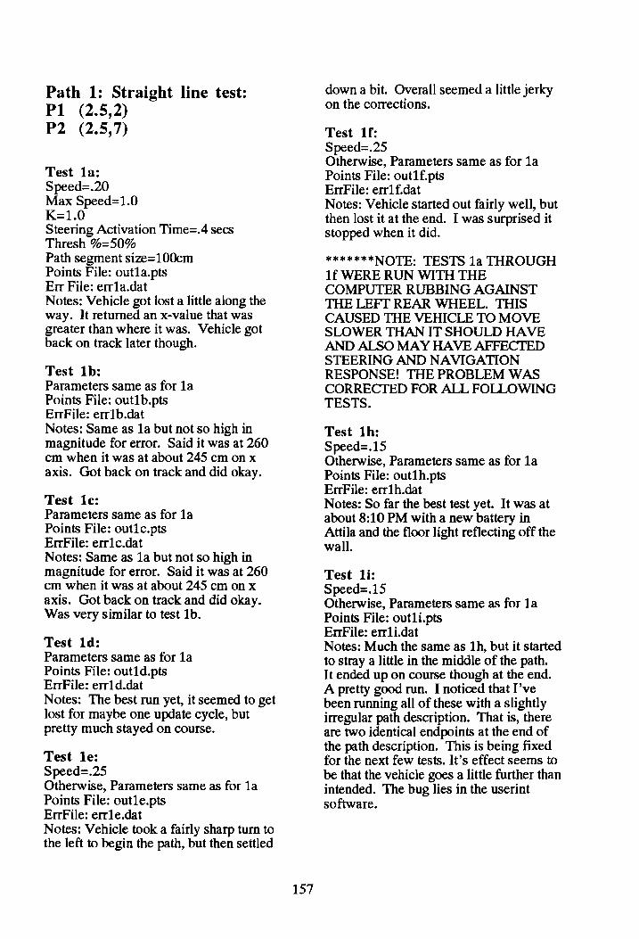
Path I: Straight line test: PI (2.5,2) P2 (2.5,7)
Test la: Speed=.20 Max Speed=1.0 K=1.0 Steering Activation Time=.4 sees Thresh %=50% Path segment size=10Ocm Points File: outla.pts Err File: errla.dat Notes: Vehicle got lost a little along the way. It returned an x-value that was greater than where it was. Vehicle got back on track later though.
Test Ib: Parameters same as for la Points File: outlb.pts ErrFile: errlb.dat Notes: Same as la but not so high in magnitude for error. Said it was at 260 cm when it was at about 245 cm on x axis. Got back on track and did okay.
Test Ie: Parameters same as for la Points File: outlc.pts ErrFile: errlc.dat Notes: Same as la but not so high in magnitude for error. Said it was at 260 cm when it was at about 245 cm on x axis. Got back on track and did okay. Was very similar to test lb.
Test Id: Parameters same as for la Points File: outld.pts ErrFile: errld.dat Notes: The best run yet, it seemed to get lost for maybe one update cycle, but pretty much stayed on course.
Test Ie: Speed=.25 Otherwise, Parameters same as for la Points File: outle.pts ErrFile: errle.dat Notes: Vehicle took a fairly sharp tum to the left to begin the path, but then settled
157
down a bit. Overall seemed a little jerky on the corrections.
Test If: Speed=.25 Otherwise, Parameters same as for la Points File: outlf.pts ErrFile: errlf.dat Notes: Vehicle started out fairly well, but then lost it at the end. I was surprised it stopped when it did.
*******NOTE: TESTS la THROUGH If WERE RUN WITH THE COMPUTER RUBBING AGAINST THE LEFT REAR WHEEL. THIS CAUSED THE VEHICLE TO MOVE SLOWER THAN IT SHOULD HAVE AND ALSO MAY HAVE AFFECTED STEERING AND NAVIGATION RESPONSE! THE PROBLEM WAS CORRECfED FOR ALL FOllOWING TESTS.
Test Ih: Speed=.15 Otherwise, Parameters same as for la Points File: outlh.pts ErrFile: errlh.dat Notes: So far the best test yet. It was at about 8:10 PM with a new battery in Attna and the floor light reflecting off the wall.
Test Ii: Speed=.15 Otherwise, Parameters same as for la Points File: outli.pts ErrFile: errli.dat Notes: Much the same as Ih, but it started to stray a little in the middle of the path. It ended up on course though at the end. A pretty good run. I noticed that I've been running all of these with a slightly irregular path description. That is, there are two identical endpoints at the end of the path description. This is being fixed for the next few tests. It's effect seems to be that the vehicle goes a little further than intended. The bug lies in the userint software.

Test 1j: Speed=.15 Otherwise, Parameters same as for la Points File: outlj.pts ErrFile: errlj.dat Notes: Another good run. The path fix made it end at y=702 cm (!!)
Test 1k: Speed=.15 Otherwise, Parameters same as for 1a Points File: outlk.pts ErrFile: err1k.dat Notes: Another good run.
Test 11: Speed=.15 Otherwise, Parameters same as for la Points File: outll.pts ErrFile: err1l.dat Notes: Another good run.
Test 1m: Speed=.20 Otherwise, Parameters same as for 1a Points File: out1m.pts ErrFile: errlm.dat Notes: Another good run at a higher speed.
Test In: Speed=.20 Otherwise, Parameters same as for la Points File: outln.pts ErrFile: errln.dat Notes: Another good run with the higher speed. It got messed up at the end. Perhaps because this time I ran after the vehicle because it takes a lot of guts to just let it run straight towards one of the transmitters trusting it will stop.
* * * * Attempts were made to run the vehicle with a speed greater than .20, but the vehicle was not able to navigate the course.
Test 10: Speed=.15 K=.95 Otherwise, Parameters same as for la Points File: out10.pts ErrFile: err10.dat
158
Notes: There was a problem from Atilla again in that it gave some incorrect coordinates and made the vehicle swerve a lot. However, the vehicle recovered and finished the path, although it seemed a little further away than it should have for y=70Ocm.
Test 1p: Speed=.15 K=.95 Otherwise, Parameters same as for 1a Points File: outl p.pts ErrFile: errl p.dat Notes: It was a very good run up until the end when it seemed to lose track of its Y position. The system was increasing its Y value up to 700 and then suddenly went to 300 or so, throwing the AGV out of control. It never recovered. This happened very close to transmitter number 3 so perhaps that had something to do the garbage.

Path 3: 2 line segment path (3 vertices) PI (4,2) P2 (2.5,4) P3 (2.5,7)
Test 3a: Speed=.12 Max Speed= 1.0 K=1.0 Steering Activation Time=.4 sees Thresh %=50% Path segment size=l00cm Points File: out3a.pts Err File: err3a.dat Notes: Seemed to be a pretty good run. It didn't get any noticeably errant position updates from AttHa
Test 3b: Parameters same as for 3a Points File: out3b.pts Err File: err3b.dat Notes: Seemed to be a pretty good run too. There seems to be some lag from the positioning system for updating the position, i.e. it seems to say that it is at 280 em when it is really at 250 cm, because it was at 280 cm 2 seconds ago.
Test 3c: Parameters same as for 3a Points File: out3c.pts Err File: err3c.dat No~: Seemed to be a pretty good run but It go sort of lost at the end. You will need to through out those points where it say Y =200 or so when Y was really 700.
Test 3d: K=l.l Otherwise, parameters same as for 3a Points File: out3d.pts Err File: err3d.dat Notes: Good run.
Test 3e: K=l.l Otherwise, parameters same as for 3a Points File: out3e.pts Err File: err3e.dat
159
Notes: Good run, except at end where it started giving funky Yvalues. Throw them out during analysis.
Test 3f: K=1.1 Otherwise, parameters same as for 3a Points File: out3f.pts Err File: err3f.dat Notes: Good run, except at end where it started giving funky Y values. Throw them out during analysis. Much the same as 3e.
Test 3g: K=0.9 Otherwise, parameters same as for 3a Points File: out3g.pts Err File: err3g.dat Notes: Good run.
Test 3h: K=0.9 Otherwise, parameters same as for 3a Points File: out3h.pts Err File: err3h.dat Notes: Good run .
Test 3i: K=0.9 Otherwise, parameters same as for 3a Points File: out3i.pts Err File: err3i.dat Notes: Not a very good run. Attila kept saying it was at x=300 when it was at x=250. It finally got back on track at the end when I thought it was all over.
Test 3j: K=1.2 Otherwise, parameters same as for 3a Points File: out3j .pts Err File: err3j.dat Notes: Attila stopped updating in the middle and vehicle strayed off course. However, AttHa got its act together and the vehicle did a good job of getting back on the path
Test 3k: K=1.2 Otherwise, parameters same as for 3a Points File: out3k.pts Err File: err3k.dat

Notes: A pretty good run overall.
Test 31: K=1.2 Otherwise, parameters same as for 3a Points File: out3l.pts Err File: err3l.dat Notes: A pretty good run.
Test 3m: K=1.1 Speed=.20 Otherwise, parameters same as for 3a Points File: out3m.pts Err File: err3m.dat Notes: A good run in that the results showed that the system was underdamped and was oscillating wildly. Next run should try to reduce K value.
Test 3D: K=0.9 Speed=.20 Otherwise, parameters same as for 3a Points File: out3n.pts Err File: err3n.dat Notes: This run showed that the speed was too fast for Attila to keep up with it. The lag was ±1 meter and this meant the vehicle was not navigating the course very well. Next try will be to slow it down a little with K= 1.0.
***** Another run was attempted at speed=.15, but this run was not successful on three attempts.
160
Path 2: 3 line segment path (4 vertices) PI (4,2) P2 (2.5,4) P3 (4,6) P4 (3,7)
Test 2a: Speed=.12 Max Speed=1.0 K=1.0 Steering Activation Time=.4 sees Thresh %=50% Path segment size=l00cm Points File: out2a.pts Err File: err2a.dat Notes: Pretty good run.
Test 2b: Parameters same as for 2a Points File: out2b.pts Err File: err2b.dat Notes: Seemed pretty gooo.
Test 2c: Parameters same as for 2a Points File: out2c.pts Err File: err2c.dat Notes: Seemed pretty good.
Test 2d: Speed=.10 K=1.2 Otherwise, parameters same as for 2a Points File: out2d.pts Err File: err2d.dat Notes: Seemed pretty good.
Test 2e: Speed=.10 K=1.2 Otherwise, parameters same as for 2a Points File: out2e.pts Err File: err2e.dat Notes: Seemed pretty good.
Test 2f: Speed=.10 K=1.2 Otherwise, parameters same as for 2a Points File: out2f.pts Err File: err2f.dat
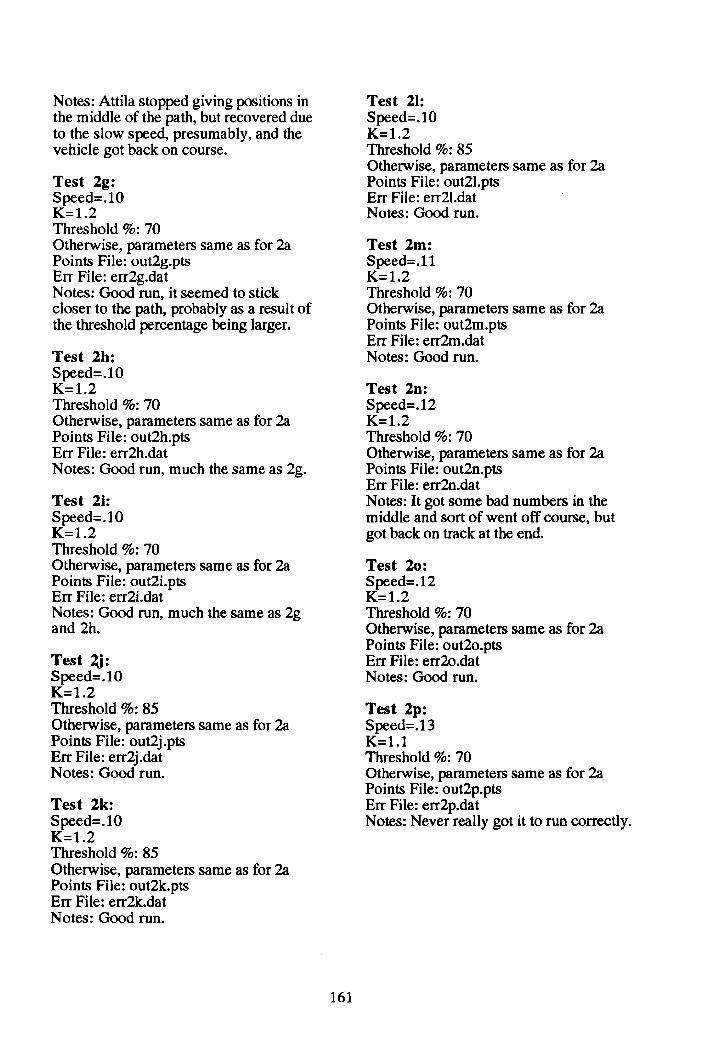
Notes: Attila stopped giving positions in the middle of the path, but recovered due to the slow speed, presumably, and the vehicle got back on course.
Test 2g: Speed=.10 K=1.2 Threshold %: 70 Otherwise, parameters same as for 2a Points File: out2g.pts Err File: err2g.dat Notes: Good run, it seemed to stick closer to the path, probably as a result of the threshold percentage being larger.
Test 2h: Speed=.10 K=1.2 Threshold %: 70 Otherwise, parameters same as for 2a Points File: out2h.pts Err File: err2h.dat Notes: Good run, much the same as 2g.
Test 2i: Speed=.10 K=1.2 Threshold %: 70 Otherwise, parameters same as for 2a Points File: out2i.pts Err File: err2i.dat Notes: Good run, much the same as 2g and 2h.
Test ~: Speed=.10 K=1.2 Threshold %: 85 Otherwise, parameters same as for 2a Points File: out2j.pts Err File: err2j.dat Notes: Good run.
Test 2k: Speed=.10 K=1.2 Threshold %: 85 Otherwise, parameters same as for 2a Points File: out2k.pts Err File: err2k.dat Notes: Good run.
161
Test 21: Speed=.10 K=1.2 Threshold %: 85 Otherwise, parameters same as for 2a Points File: out2l.pts Err File: err2l.dat Notes: Good run.
Test 2m: Speed=.11 K=1.2 Threshold %: 70 Otherwise, parameters same as for 2a Points File: out2m.pts Err File: err2m.dat Notes: Good run.
Test 20: Speed=.12 K=1.2 Threshold %: 70 Otherwise, parameters same as for 2a Points File: out2n.pts Err File: err2n.dat Notes: It got some bad numbers in the middle and sort of went off course, but got back on track at the end.
Test 20: Speed=.12 K=1.2 Threshold %: 70 Otherwise, parameters same as for 2a Points File: out20.pts Err File: err20.dat Notes: Good run.
Test 2p: Speed=.13 K=1.1 Threshold %: 70 Otherwise, parameters same as for 2a Points File: out2p.pts Err File: err2p.dat Notes: Never really got it to run correctly.

VITA
Jeff Fithian was born on August 15, 1966 to Ephraim B. and Patricia L. Fithian,
who currently reside in Orefield, Pennsylvania. He attended high school at Parkland High
School in Orefield, Pennsylvania (1981-1984). He attended Drexel University from
September 1984 to June 1986 majoring in Computer Engineering before transferring to
Virginia Tech to graduate with a Bachelor of Science in Industrial Engineering and
Operations Research in May of 1989. After working in Europe for two years, he returned
to Virginia Tech in August of 1991 to pursue a Master of Science in Industrial and Systems
Engineering with a concentration in Manufacturing Systems. After graduation, he will be
working in Munich, Germany with Siemens AG as a manufacturing engineer.
Je E. FIthIan
162

ABSTRACT
The purpose of this research is to examine the feasibility of a laser-based
positioning system for navigation of an autonomous, automated guided vehicle. The
system differs from existing systems in that there is no dead-reckoning used during
navigation, thus avoiding the pitfalls of dead-reckoning as a navigation method. The
system also requires little prior structuring of the environment and can navigate the vehicle
in real-time.
Software was written to allow the user to easily generate and modify paths using
existing PC-based drawing and/or CAD software. In addition, menu-driven navigation
software was written which allows the user to modify navigation parameters during testing
to determine their effect on navigational accuracy. Tests were run of three different paths,
and the results were presented in graphical form to the reader. In addition, the average
absolute path error was recorded for each test. The parameters used for each test and a
discussion of the tests are provided for the reader also. A full listing of the program code
developed for this system is presented in the thesis document.
The results showed that it is possible to navigate a vehicle around a pre-defined path
with acceptable accuracy using a laser-based positioning system as the only navigation
method. The average absolute path error for a complex path was approximately ±10
centimeters at a vehicle speed of approximately one meter per second. Straight line paths
gave better errors and allowed for a higher velocity, but are not indicative of typical vehicle
paths encountered in an industrial setting.
The current system showed some reliability and range problems, but when
functioning it proved to be very accurate. A new laser-based positioning system currently
under development will address many of the problems encountered in this research.