a large scale benchmark and an inclusion-based …

A Large Scale Benchmark and an Inclusion-Based Algorithm forContinuous Collision Detection

BOLUN WANG∗, Beihang University and New York University

ZACHARY FERGUSON∗, New York University

TESEO SCHNEIDER, New York University and University of Victoria

XIN JIANG, Beihang University and Peng Cheng Laboratory in Shenzhen

MARCO ATTENE, IMATI - CNR

DANIELE PANOZZO, New York University

Numberof

FalsePositives

OURS IRF UIRF TCCDMSRF RP RRP BSC FPRF

1

100

10k

1M

Numberof

FalseNegatives


1

100

10k

1M

Average

Tim

e(µs)


1

10

100

1000

Fig. 1. An overview of the results of our study of different CCD methods run on 60 million queries (both vertex-face and edge-edge). For each method, we show

the number of false positives (i.e., the method detects a collision where there is none), the number of false negatives (i.e., the method misses a collision), and

the average run time. Each plot reports results in a logarithmic scale. False positives and negatives are computed with respect to the ground truth computed

using Mathematica [Wolfram Research Inc. 2020]. Acronyms are defined in Section 4.2.

We introduce a large scale benchmark for continuous collision detection(CCD) algorithms, composed of queries manually constructed to highlightchallenging degenerate cases and automatically generated using existingsimulators to cover common cases. We use the benchmark to evaluate theaccuracy, correctness, and efficiency of state-of-the-art continuous collisiondetection algorithms, both with and without minimal separation.

We discover that, despite the widespread use of CCD algorithms, existingalgorithms are either: (1) correct but impractically slow, (2) efficient butincorrect, introducing false negatives which will lead to interpenetration, or(3) correct but over conservative, reporting a large number of false positiveswhich might lead to inaccuracies when integrated in a simulator.

By combining the seminal interval root finding algorithm introducedby Snyder in 1992 with modern predicate design techniques, we propose asimple and efficient CCD algorithm. This algorithm is competitive with stateof the art methods in terms of runtime while conservatively reporting the

∗Joint first authors

Authors’ addresses: Bolun Wang, LMIB & NLSDE & School of Mathematical Sciences &Shenyuan Honor College, Beihang University, New York University, [email protected]; Zachary Ferguson, New York University, [email protected], [email protected];Teseo Schneider, New York University, University of Victoria; Xin Jiang, LMIB &NLSDE& School of Mathematical Sciences, Beihang University, Peng Cheng Laboratoryin Shenzhen; Marco Attene, IMATI - CNR; Daniele Panozzo, New York University,[email protected].

Permission to make digital or hard copies of all or part of this work for personal orclassroom use is granted without fee provided that copies are not made or distributedfor profit or commercial advantage and that copies bear this notice and the full citationon the first page. Copyrights for components of this work owned by others than theauthor(s) must be honored. Abstracting with credit is permitted. To copy otherwise, orrepublish, to post on servers or to redistribute to lists, requires prior specific permissionand/or a fee. Request permissions from [email protected].© 2021 Copyright held by the owner/author(s). Publication rights licensed to ACM.0730-0301/2021/1-ART1 $15.00https://doi.org/10.1145/3460775

time of impact and allowing explicit trade off between runtime efficiencyand number of false positives reported.

CCS Concepts: · Computing methodologies → Collision detection;Physical simulation.

Additional Key Words and Phrases: continuous collision detection, compu-

tational geometry, physically based animation

ACM Reference Format:

Bolun Wang, Zachary Ferguson, Teseo Schneider, Xin Jiang, Marco Attene,and Daniele Panozzo. 2021. A Large Scale Benchmark and an Inclusion-Based Algorithm for Continuous Collision Detection. ACM Trans. Graph. 1,1, Article 1 (January 2021), 16 pages. https://doi.org/10.1145/3460775

1 INTRODUCTION

Collision detection and response are two separate, yet intercon-nected, problems in computer graphics and scientific computing.Collision detection specializes in finding when and if two objectscollide, while collision response uses this information to deform theobjects following physical laws. A large research effort has beeninvested in the latter problem, assuming that collision detectioncan be solved reliably and efficiently. In this study we focus on theformer, using an experimental approach based on large scale testing.We use existing collision response methods to generate collision de-tection queries to investigate the pros and cons of existing collisiondetection algorithms.

Static collision detection is popular in interactive applications dueto its efficiency, its inability to detect collisions between fast movingobjects passing through each other (tunneling) hinders its applicabil-ity. To address this limitation, continuous collision detection (CCD)methods have been introduced: by solving a more computationally

ACM Trans. Graph., Vol. 1, No. 1, Article 1. Publication date: January 2021.

https://doi.org/10.1145/3460775

https://doi.org/10.1145/3460775

1:2 • Bolun Wang, Zachary Ferguson, Teseo Schneider, Xin Jiang, Marco Attene, and Daniele Panozzo

intensive problem, usually involving finding roots of a low-degreepolynomial, these algorithms can detect any collision happening ina time step, often assuming linear trajectories.The added robustness makes this family of algorithms popular,

but they can still fail due to floating-point rounding errors. Floatingpoint failures are of two types: false negatives, i.e., missed collisions,which lead to interpenetration, and false positives, i.e., detectingcollisions when there are none.

Most collision response algorithms can tolerate minor imperfec-tions, using heuristics to recover from physically invalid states (inreality, objects cannot inter-penetrate). However, these heuristicshave parameters that needs to be tuned for every scene to ensurestability and faithfulness in the simulation [Li et al. 2020]. Recently,the collision response problem has been reformulated to avoid theuse of heuristics, and the corresponding parameter tuning, by disal-lowing physically invalid configurations [Li et al. 2020]. For instance,in the attached video, the method in [Li et al. 2020] cannot recoverfrom interpenetration after the CCD misses a collision leading toan unnatural łstickingž and eventual failure of the simulation. Thiscomes with a heavier burden on the CCD algorithm used, whichshould never report false negatives.We introduce a large benchmark of CCD queries with ground

truth computed using the exact, symbolic solver ofMathematica [Wol-fram Research Inc. 2020], and evaluate the correctness (lack of falsenegatives), conservatiness (false positive count), and runtime ef-ficiency of existing state of the art algorithms. The benchmark iscomposed of both manually designed queries to identify degener-ate cases (building upon [Erleben 2018]) and a large collection ofreal-world queries extracted from simulation sequences. On thealgorithmic side, we select representative algorithms from the threemain approaches existing in the literature for CCD root-finding:inclusion-based bisection methods [Redon et al. 2002; Snyder et al.1993], numerical methods [Vouga et al. 2010; Wang et al. 2015], andexact methods [Brochu et al. 2012; Tang et al. 2014]. Thanks to ourbenchmark, we identified missing cases that were not handled byprevious methods, and we did a best effort to fix the correspondingalgorithms and implementations to account for these cases.The surprising conclusion of this study (Section 4.2) is that the

majority of the existing CCD algorithms produce false negatives, ex-cept three: (1) symbolic solution of the system and evaluation withexact arithmetic computed using Mathematica [Wolfram ResearchInc. 2020], (2) Bernstein sign classification (BSC) with conservativeerror analysis [Wang et al. 2015], and (3) inclusion-based bisectionroot finding [Redon et al. 2002; Snyder et al. 1993]. (1) is extremelyexpensive and, while it can be used for generating the ground truth,it is impractical in simulation applications. (2) is efficient but gener-ates many false positives and the number of false positives dependson the geometric configuration and velocities involved. (3) is one ofthe oldest methods proposed for CCD. It is slow compared to stateof the art algorithms, but it is correct and allows precise control ofthe trade-off between false positives and computational cost.This extensive analysis and benchmark inspired us to introduce

a specialization of the classical inclusion-based bisection algorithmproposed in [Snyder 1992] to the specific case of CCD for triangu-lar meshes (Section 5). The major changes are: a novel inclusionfunction, an efficient strategy to perform bisection, and the ability

to find CCD roots with minimal separation (Section 6). Our novelinclusion function:

(1) is tighter leading to smaller boxes on average thus makingour method more accurate (i.e., less false positive);

(2) reduces the root-finding problem into the iterative evaluationof a Boolean function, which allows replacing explicit intervalarithmetic with a more efficient floating point filtering;

(3) can be vectorized with AVX2 instructions.

With these modifications, our inclusion-based bisection algorithmis only 3× slower on average than the fastest inaccurate CCD al-gorithm. At the same time it is provably conservative, provides acontrollable ratio of false positives (within reasonable numericallimits), supports minimal separation, and reports the time of impact.We also discuss how to integrate minimal separation CCD in algo-rithms employing a line search to ensure the lack of intersections,which are common in locally injective mesh parametrization andhave been recently introduced in physical simulation by Li et al.[2020].

Our dataset is available at the NYU Faculty Digital Archive, whilethe implementation of all the algorithms compared in the bench-mark, a reference implementation of our novel inclusion-basedbisection algorithm, and scripts to reproduce all results (Section 4)are available at https://github.com/Continuous-Collision-Detection.We believe this dataset will be an important element to supportresearch in efficient and correct CCD algorithms, while our novelinclusion-based bisection algorithm is a practical solution that willallow researchers and practitioners to robustly check for collisionsin applications where a 3× slowdown in the CCD (which is usuallyonly one of the expensive steps of a simulation pipeline) will bepreferable over the risk of false negatives or the need to tune CCDparameters.

2 RELATED WORK

We present a brief overview of the previous works on continuous col-lision detection for triangle meshes. Our work focuses only on CCDfor deformable trianglemeshes andwe thus exclude discussingmeth-ods approximating collisions using proxies (e.g., Hubbard [1995];Mirtich [1996]).

Inclusion-Based Root-Finding. The generic algorithm in the sem-inal work of Snyder [1992] on interval arithmetic for computergraphics is a conservative way to find collisions [Redon et al. 2002;Snyder et al. 1993; Von Herzen et al. 1990]. This approach uses in-clusion functions to certify the existence of roots within a domain,using a bisection partitioning strategy. Surprisingly, this approachis not used in recent algorithms despite being provably conservativeand simple. Our algorithm is based on this approach, but with twomajor extensions to improve its efficiency (Section 5).

Numerical Root-Finding. The majority of CCD research focuseson efficient and accurate ways of computing roots of special cubicpolynomials. Among these, a most popular cubic solver approachis introduced by Provot [1997], in which a cubic equation is solvedto check for coplanarity, and then the overlapping occurrence isvalidated to determine whether a collision actually occurs. Refinedconstructions based on this idea have been introduced for rigid [Kim


https://archive.nyu.edu/handle/2451/61518

https://github.com/Continuous-Collision-Detection

A Large Scale Benchmark and an Inclusion-Based Algorithm for Continuous Collision Detection • 1:3

and Rossignac 2003; Redon et al. 2002] and deformable [Hutter andFuhrmann 2007; Tang et al. 2011] bodies. However, all of these algo-rithms are based on floating-point arithmetic, requiring numericalthresholds to account for the unavoidable rounding errors in theiterative root-finding procedure. In fact, even if the cubic polynomialis represented exactly, its roots are generally irrational and thusnot representable with floating-point numbers. Unfortunately, thenumerical thresholds make these algorithms robust only for specificscenarios, and they can in general introduce false negatives. Our ap-proach has a moderately higher runtime than these algorithms, butit is guaranteed to avoid false negatives without parameter tuning.We benchmark Provot [1997] using the implementation of Vougaet al. [2010] in Section 4.For most applications, false positives are less problematic than

false negatives since a false negative will miss a collision, leadingto interpenetration and potentially breaking the simulation. Tanget al. [2010] propose a simple and effective filter which can reduceboth the number of false positives and the elementary tests betweenthe primitives. Wang [2014] and Wang et al. [2015] improve itsreliability by introducing forward error analysis, in which errorbounds for floating-point computation are used to eliminate falsepositives. We benchmark the representative method of Wang et al.[2015] in Section 4.

Exact Root-Finding. Brochu et al. [2012] and Tang et al. [2014]introduce algorithms relying on exact arithmetic to provide ex-act continuous collision detection. However, after experimentingwith their implementations and carefully studying their algorithms,we discovered that they cannot always provide the exact answer(Section 4). Brochu et al. [2012] rephrase the collision problem ascounting the number of intersections between a ray and the bound-ary of a subset of R3 bounded by bilinear faces. The ray castingand polygonal construction can be done using rational numbers (ormore efficiently with floating point expansions) to avoid floating-point rounding errors. In [Tang et al. 2014] the CCD queries arereduced to the evaluation of the signs of Bernstein polynomials andalgebraic expressions, using a custom root finding algorithm. Ouralgorithm uses the geometric formulation proposed in [Brochu et al.2012], but uses a bisection strategy instead of ray casting to findthe roots. We benchmark both [Brochu et al. 2012] and [Tang et al.2014] in Section 4.

Minimal Separation. Minimal separation CCD (MSCCD) [Harmonet al. 2011; Lu et al. 2019; Provot 1997; Stam 2009] reports collisionswhen two objects are at a (usually small) user-specified distance.These approaches have two main applications: (1) a minimal sepa-ration is useful in fabrication settings to ensure that the fabricationerrors will not lead to penetrations, and (2) a minimal separationcan ensure that, after floating-point rounding, two objects are stillnot intersecting, an invariant which must be preserved by certainsimulation codes [Harmon et al. 2011; Li et al. 2020]. We bench-mark [Harmon et al. 2011] in Section 6.2. Our algorithm supportsa novel version of minimal separation, where we use the 𝐿∞ norminstead of 𝐿2 (Section 6.1).

Collision Culling. An orthogonal problem is efficient high-levelcollision culling to quickly filter out primitive pairs that do not

collide in a time step. Since in this case it is tolerable to have manyfalse positives, it is easy to find conservative approaches that areguaranteed to not discard potentially intersecting pairs [Curtis et al.2008; Govindaraju et al. 2005; Mezger et al. 2003; Pabst et al. 2010;Provot 1997; Schvartzman et al. 2010; Tang et al. 2009a, 2008; Volinoand Thalmann 1994; Wong and Baciu 2006; Zhang et al. 2007; Zhengand James 2012]. Any of these approaches can be used as a prepro-cessing step to any of the CCD methods considered in this study toimprove performance.

Generalized Trajectories. The linearization of trajectories com-monly used in collision detection is a well-established, practicalapproximation, ubiquitous in existing codes. There are, however,methods that can directly detect collisions between objects follow-ing polynomial trajectories [Pan et al. 2012] or rigid motions [Canny1986; Redon et al. 2002; Tang et al. 2009b; Zhang et al. 2007], andavoid the approximation errors due to the linearization. Our algo-rithm currently does not support curved trajectories and we believethis is an important direction for future work.

3 PRELIMINARIES AND NOTATION

Assuming that the objects are represented using triangular meshesand that every vertex moves in a linear trajectory in each time step,the first collision between moving triangles can happen either whena vertex hits a triangle, or when an edge hits another edge.Thus a continuous collision detection algorithm is a procedure

that, given a vertex-face or edge-edge pair, equipped with their lin-ear trajectories, determines if and when they will touch. Formally,for the vertex-face CCD, given a vertex 𝑝 and a face with vertices𝑣1, 𝑣2, 𝑣3 at two distinct time steps 𝑡0 and 𝑡1 (we use the super-script notation to denote the time, i.e., 𝑝0 is the position of 𝑝 at 𝑡0),the goal is to determine if at any point in time between 𝑡0 and 𝑡1

the vertex is contained in the moving face. Similarly for the edge-edge CCD the algorithm aims to find if there exists a 𝑡 ∈ [𝑡0, 𝑡1]where the two moving edges (𝑝𝑡1, 𝑝

𝑡2) and (𝑝

𝑡3, 𝑝

𝑡4) intersect. We will

briefly overview and discuss the pros and cons of the two majorformulations present in the literature to address the CCD problem:multi-variate and univariate.

Multivariate CCD Formulation. The most direct way of solvingthis problem is to parametrize the trajectories with a parameter𝑡 ∈ [0, 1] (i.e., 𝑝𝑖 (𝑡) = (1 − 𝑡)𝑝0𝑖 + 𝑡𝑝

1𝑖 and 𝑣𝑖 (𝑡) = (1 − 𝑡)𝑣0𝑖 + 𝑡𝑣

1𝑖 )

and write a multivariate polynomial whose roots correspond tointersections. That is finding the roots of

𝐹vf : Ωvf = [0, 1] × {𝑢, 𝑣 ⩾ 0|𝑢 + 𝑣 ⩽ 1} → R3

with

𝐹vf (𝑡,𝑢, 𝑣) = 𝑝 (𝑡) −(

(1 − 𝑢 − 𝑣)𝑣1 (𝑡) + 𝑢𝑣2 (𝑡) + 𝑣𝑣3 (𝑡))

, (1)

for the vertex-face case. Similarly for the edge-edge case the goal isto find the roots of

𝐹ee : Ωee = [0, 1] × [0, 1]2 → R3

with

𝐹ee (𝑡,𝑢, 𝑣) =(

(1−𝑢)𝑝1 (𝑡) +𝑢𝑝2 (𝑡))

−(

(1− 𝑣)𝑝3 (𝑡) + 𝑣𝑝4 (𝑡))

. (2)

In other words, the CCD problem reduces to determining if 𝐹 has aroot in Ω (i.e., there is a combination of valid 𝑡,𝑢, 𝑣 for which the



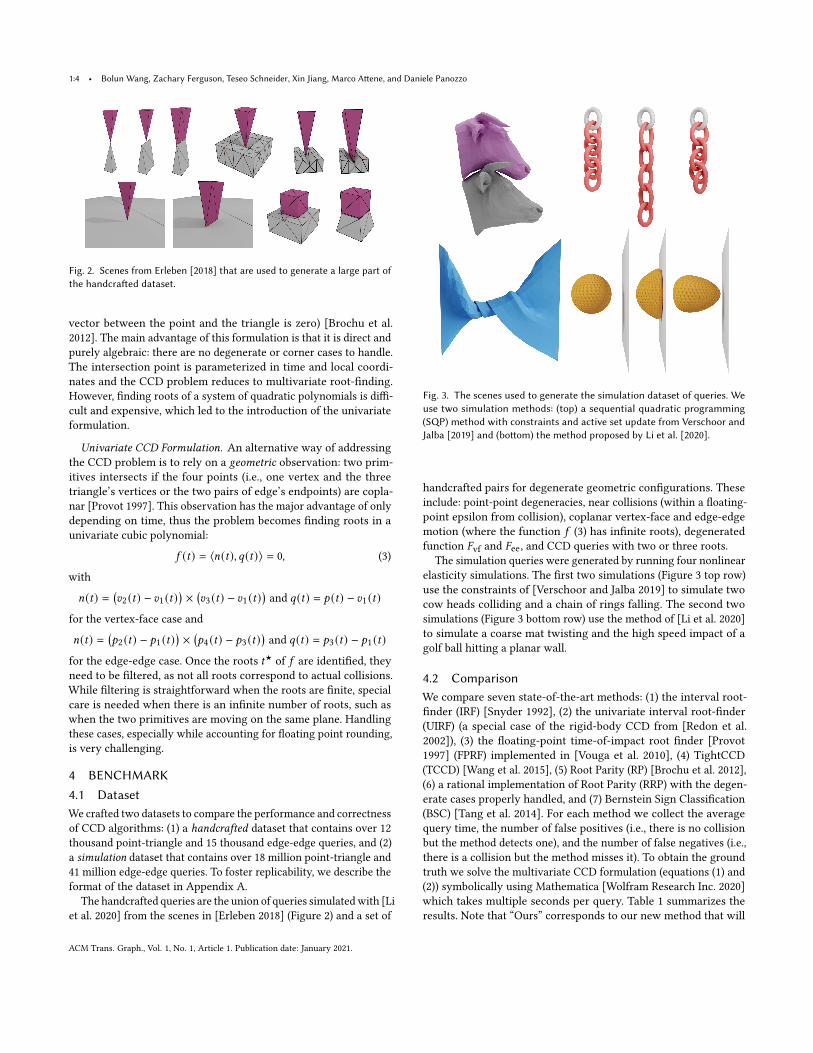
Fig. 2. Scenes from Erleben [2018] that are used to generate a large part of

the handcrafted dataset.

vector between the point and the triangle is zero) [Brochu et al.2012]. The main advantage of this formulation is that it is direct andpurely algebraic: there are no degenerate or corner cases to handle.The intersection point is parameterized in time and local coordi-nates and the CCD problem reduces to multivariate root-finding.However, finding roots of a system of quadratic polynomials is diffi-cult and expensive, which led to the introduction of the univariateformulation.

Univariate CCD Formulation. An alternative way of addressingthe CCD problem is to rely on a geometric observation: two prim-itives intersects if the four points (i.e., one vertex and the threetriangle’s vertices or the two pairs of edge’s endpoints) are copla-nar [Provot 1997]. This observation has the major advantage of onlydepending on time, thus the problem becomes finding roots in aunivariate cubic polynomial:

𝑓 (𝑡) = ⟨𝑛(𝑡), 𝑞(𝑡)⟩ = 0, (3)

with

𝑛(𝑡) =(

𝑣2 (𝑡) − 𝑣1 (𝑡))

×(

𝑣3 (𝑡) − 𝑣1 (𝑡))

and 𝑞(𝑡) = 𝑝 (𝑡) − 𝑣1 (𝑡)

for the vertex-face case and

𝑛(𝑡) =(

𝑝2 (𝑡) − 𝑝1 (𝑡))

×(

𝑝4 (𝑡) − 𝑝3 (𝑡))

and 𝑞(𝑡) = 𝑝3 (𝑡) − 𝑝1 (𝑡)

for the edge-edge case. Once the roots 𝑡★ of 𝑓 are identified, theyneed to be filtered, as not all roots correspond to actual collisions.While filtering is straightforward when the roots are finite, specialcare is needed when there is an infinite number of roots, such aswhen the two primitives are moving on the same plane. Handlingthese cases, especially while accounting for floating point rounding,is very challenging.

4 BENCHMARK

4.1 Dataset

We crafted two datasets to compare the performance and correctnessof CCD algorithms: (1) a handcrafted dataset that contains over 12thousand point-triangle and 15 thousand edge-edge queries, and (2)a simulation dataset that contains over 18 million point-triangle and41 million edge-edge queries. To foster replicability, we describe theformat of the dataset in Appendix A.

The handcrafted queries are the union of queries simulatedwith [Liet al. 2020] from the scenes in [Erleben 2018] (Figure 2) and a set of

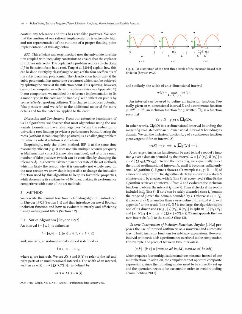
Fig. 3. The scenes used to generate the simulation dataset of queries. We

use two simulation methods: (top) a sequential quadratic programming

(SQP) method with constraints and active set update from Verschoor and

Jalba [2019] and (bottom) the method proposed by Li et al. [2020].

handcrafted pairs for degenerate geometric configurations. Theseinclude: point-point degeneracies, near collisions (within a floating-point epsilon from collision), coplanar vertex-face and edge-edgemotion (where the function 𝑓 (3) has infinite roots), degeneratedfunction 𝐹vf and 𝐹ee, and CCD queries with two or three roots.

The simulation queries were generated by running four nonlinearelasticity simulations. The first two simulations (Figure 3 top row)use the constraints of [Verschoor and Jalba 2019] to simulate twocow heads colliding and a chain of rings falling. The second twosimulations (Figure 3 bottom row) use the method of [Li et al. 2020]to simulate a coarse mat twisting and the high speed impact of agolf ball hitting a planar wall.

4.2 Comparison

We compare seven state-of-the-art methods: (1) the interval root-finder (IRF) [Snyder 1992], (2) the univariate interval root-finder(UIRF) (a special case of the rigid-body CCD from [Redon et al.2002]), (3) the floating-point time-of-impact root finder [Provot1997] (FPRF) implemented in [Vouga et al. 2010], (4) TightCCD(TCCD) [Wang et al. 2015], (5) Root Parity (RP) [Brochu et al. 2012],(6) a rational implementation of Root Parity (RRP) with the degen-erate cases properly handled, and (7) Bernstein Sign Classification(BSC) [Tang et al. 2014]. For each method we collect the averagequery time, the number of false positives (i.e., there is no collisionbut the method detects one), and the number of false negatives (i.e.,there is a collision but the method misses it). To obtain the groundtruth we solve the multivariate CCD formulation (equations (1) and(2)) symbolically using Mathematica [Wolfram Research Inc. 2020]which takes multiple seconds per query. Table 1 summarizes theresults. Note that łOursž corresponds to our new method that will



Table 1. Summary of the average runtime in 𝜇𝑠 (t), number of false positive

(FP), and number of false negative (FN) for the six competing methods.

Handcrafted Dataset (12K) ś Vertex-Face CCD

IRF UIRF FPRF TCCD RP RRP BSC MSRF Ours

t 14942.40 124242.00 2.18 0.38 1.41 928.08 176.17 12.90 1532.54FP 87 146 9 903 3 0 11 16 108FN 0 0 70 0 5 5 13 386 0

Handcrafted Dataset (15K)ś Edge-Edge CCD


t 12452.60 18755.80 0.48 0.33 2.33 1271.32 121.80 2.72 3029.83FP 141 268 5 404 3 0 28 14 214FN 0 0 147 0 8 8 47 335 0

Simulation Dataset (18M) ś Vertex-Face CCD


t 115.89 6191.98 7.53 0.24 0.25 1085.13 34.21 51.07 0.74FP 2 18 0 95638 0 0 23015 75 2FN 0 0 5184 0 0 0 0 0 0

Simulation Dataset (41M) ś Edge-Edge CCD


t 215.80 846.57 0.23 0.23 0.37 1468.70 12.87 10.39 0.78FP 71 16781 0 82277 0 0 4593 228 17FN 0 0 2317 0 7 7 27 1 0

be introduced and discussed in Section 5 and MSRF is a minimumseparation CCD discussed in Section 6.2.

IRF. The inclusion-based root-finding described in [Snyder 1992]can be applied to both the multivariate and univariate CCD. Forthe multivariate case we can simply initialize the parameters of 𝐹(i.e., 𝑡,𝑢, 𝑣) with the size of the domain Ω, evaluate 𝐹 and check ifthe origin is contained in the output interval [Snyder et al. 1993].If it is, we sequentially subdivide the parameters (thus shrinkingthe size of the intervals of 𝐹 ) until a user-tolerance 𝛿 is reached.In our comparison we use 𝛿 = 10−6. The major advantage of thisapproach is that it is guaranteed to be conservative: it is impossibleto shrink the interval of 𝐹 to zero. A second advantage is that auser can easily trade accuracy (number of false positives) for effi-ciency by simply increasing the tolerance 𝛿 (Appendix D). The maindrawback is that bisecting Ω in the three dimensions makes thealgorithm slow, and the use of interval arithmetic further increasesthe computational cost and prevents the use of certain compileroptimization techniques (such as instruction reordering). We imple-ment this approach using the numerical type provided by the Boostinterval library [Schling 2011].

UIRF. [Snyder 1992] can also be applied to the univariate functionin Equation (3) by using the same subdivision technique on thesingle variable 𝑡 (as in [Redon et al. 2002] but for linear trajectories).The result of this step is an interval containing the earliest rootin 𝑡 which is then plugged inside a geometric predicate to checkif the primitives intersect in that interval. While finding the rootswith this approach might, at a first glance, seem easier than in themulti-variate case and thus more efficient, this is not the case in ourexperiments. If the polynomial has infinite roots, this algorithm willhave to refine the entire domain to the maximal allowed resolution,and check the validity of each interval, making it correct but very

slow on degenerate cases (Appendix D). This results in a longeraverage runtime than its multivariate counterpart. Additionally, itis impossible to control the accuracy of the other two parameters(i.e., 𝑢, 𝑣), thus introducing more false positives.

FPRF. Vouga et al. [2010] aim to solve the univariate CCD problemusing only floating-point computation. To mitigate false negatives,the method uses a numerical tolerance 𝜂 (Appendix E) shows how𝜂 affects running time, the false positive, and negative). The majorlimitations are that the number of false positives cannot be directlycontrolled as it depends on the relative position of the input prim-itives and that false negatives can appear if the parameter is nottuned accordingly to the objects velocity and scale. Additionally,the reference implementation does not handle the edge-edge CCDwhen the two edges are parallel. This method is one of the fastest,which makes it a very popular choice in many simulation codes.

TCCD. TightCCD is a conservative floating-based implementa-tion of Tang et al. [2014]. It uses the univariate formulation coupledwith three inequality constraints (two for the edge-edge case) toensure that the univariate root is a CCD root. The algorithm ex-presses the cubic polynomial 𝑓 as a product and sum of three loworder polynomials in Bernstein form. With this reformulation theCCD problem becomes checking if univariate Bernstein polynomi-als are positive, which can be done by checking some specific points.This algorithm is extremely fast but introduces many false positiveswhich are impossible to control. In our benchmark, this is the onlynon-interval method without false negatives. The major limitationof this algorithm is that it always detects collision if the primitivesare moving in the same plane, independently from their relativeposition.

RP and RRP. These two methods use the multivariate formulation𝐹 (equations (1) and (2)). The main idea is that the parity of theroots of 𝐹 can be reduced to a ray casting problem. Let 𝜕Ω be theboundary of Ω, the algorithm shoots a ray from the origin andcounts the parity of the intersection between the ray and 𝐹 (𝜕Ω)

which corresponds to the parity of the roots of 𝐹 . Parity is howeverinsufficient for CCD: these algorithms cannot differentiate betweenzero roots (no collision) and two roots (collision), since they havethe same parity. We note that this is a rare case happening onlywith sufficiently large time-steps and/or velocities: we found 13(handcrafted dataset) and 7 (simulation dataset) queries where thesemethods report a false negative.

We note that the algorithm described in [Brochu et al. 2012] (andits reference implementation) does not handle some degeneratecases leading to both false negatives and positives. For instance,in Appendix B, we show an example of a łhourglassž configura-tion where RP misses the collision, generating a false negative. Toovercome this limitations and provide a fair comparison to thesetechniques, we implemented a naïve version of this algorithm thathandles all the degenerate cases using rational numbers to sim-plify the coding (see the additional materials). We opted for thisrational implementation since properly handling the degeneraciesusing floating-point requires designing custom higher precisionpredicates for all cases. The main advantage of this method is thatit is exact (when the degenerate cases are handled) as it does not



contain any tolerance and thus has zero false positives. We notethat the runtime of our rational implementation is extremely highand not representative of the runtime of a proper floating pointimplementation of this algorithm.

BSC. This efficient and exact method uses the univariate formula-tion coupled with inequality constraints to ensure that the coplanarprimitives intersects. The coplanarity problem reduces to checkingif 𝑓 in Bernstein form has a root. Tang et al. [2014] explain how thiscan be done exactly by classifying the signs of the four coefficients ofthe cubic Bernstein polynomial. The classification holds only if thecubic polynomial has monotone curvature; which can be achievedby splitting the curve at the inflection point. This splitting, however,cannot be computed exactly as it requires divisions (Appendix C).In our comparison, we modified the reference implementation to fixa minor typo in the code and to handle 𝑓 with inflection points byconservatively reporting collision. This change introduces potentialfalse positives, and we refer to the additional material for moredetails and for the patch we applied to the code.

Discussion and Conclusions. From our extensive benchmark ofCCD algorithms, we observe that most algorithms using the uni-variate formulation have false negatives. While the reduction tounivariate root findings provides a performance boost, filtering theroots (without introducing false positives) is a challenging problemfor which a robust solution is still elusive.Surprisingly, only the oldest method, IRF, is at the same time

reasonably efficient (e.g., it does not take multiple seconds per queryas Mathematica), correct (i.e., no false negatives), and returns a smallnumber of false positives (which can be controlled by changing thetolerance 𝛿). It is however slower than other state of the art methods,which is likely the reason why it is currently not widely used. Inthe next section we show that it is possible to change the inclusionfunction used by this algorithm to keep its favorable properties,while decreasing its runtime by ∼250 times, making its performancecompetitive with state of the art methods.

5 METHOD

We describe the seminal bisection root-finding algorithm introducedin [Snyder 1992] (Section 5.1) and then introduce our novel Booleaninclusion function and how to evaluate it exactly and efficientlyusing floating point filters (Section 5.2).

5.1 Solve Algorithm [Snyder 1992]

An interval 𝑖 = [𝑎, 𝑏] is defined as

𝑖 = [𝑎, 𝑏] = {𝑥 |𝑎 ⩽ 𝑥 ⩽ 𝑏, 𝑥, 𝑎, 𝑏 ∈ R},

and, similarly, an 𝑛-dimensional interval is defined as

𝐼 = 𝑖1 × · · · × 𝑖𝑛,

where 𝑖𝑘 are intervals. We use L(𝑖) and R(𝑖) to refer to the left andright parts of an unidimensional interval 𝑖 . The width of an interval,written as𝑤 (𝑖) = 𝑤 ( [L(𝑖),R(𝑖)]), is defined by

𝑤 (𝑖) = L(𝑖) − R(𝑖)

0 1

Ig

g

0 1

I0

0 1

Ig

g

0.50

I1 I2

0.5

1

0 1

Ig

g

0.50.25

I3 I4

0.5

0.25

0

ℓ = 0 ℓ = 1 ℓ = 2

Fig. 4. 1D illustration of the first three levels of the inclusion based root-

finder in [Snyder 1992].

and similarly, the width of an 𝑛-dimensional interval

𝑤 (𝐼 ) = max𝑘={1,...,𝑛}

𝑤 (𝑖𝑘 ).

An interval can be used to define an inclusion function. For-mally, given an𝑚-dimensional interval𝐷 and a continuous function𝑔 : R𝑚 → R𝑛 , an inclusion function for 𝑔, written□𝑔, is a functionsuch that

∀𝑥 ∈ 𝐷 𝑔(𝑥) ∈□𝑔(𝐷).

In other words, □𝑔(𝐷) is a 𝑛-dimensional interval bounding therange of 𝑔 evaluated over an𝑚-dimensional interval 𝐷 bounding itsdomain. We call the inclusion function□𝑔 of a continuous function𝑔 convergent if for an interval 𝑋

𝑤 (𝑋 ) → 0 =⇒ 𝑤(

□𝑔(𝑋 ))

→ 0.

A convergent inclusion function can be used to find a root of a func-tion 𝑔 over a domain bounded by the interval 𝐼0 = [L(𝑥1),R(𝑥1)] ×· · · × [L(𝑥𝑚),R(𝑥𝑚)]. To find the roots of 𝑔, we sequentially bisectthe initial𝑚-dimensional interval 𝐼0, until it becomes sufficientlysmall (Algorithm 1). Figure 4 shows a 1D example (i.e., 𝑔 : R→ R) ofa bisection algorithm. The algorithm starts by initializing a stack 𝑆of intervals to be checked with 𝐼0 (line 3). At every level ℓ (line 5), thealgorithm retrieves an interval 𝐼 from 𝑆 and evaluates the inclusionfunction to obtain the interval 𝐼𝑔 (line 7). Then it checks if the root isincluded in 𝐼𝑔 (line 8). If not 𝐼 can be safely discarded since 𝐼𝑔 boundsthe range of 𝑔 over the domain bounded by 𝐼 . Otherwise (0 ∈ 𝐼𝑔 ),it checks if𝑤 (𝐼 ) is smaller than a user-defined threshold 𝛿 . If so itappends 𝐼 to the result (line 10). If 𝐼 is too large, the algorithm splitsone of its dimensions (e.g., [L(𝑥1),R(𝑥1)] is split in [L(𝑥1), 𝑥1]and [𝑥1,R(𝑥1)] with 𝑥1 = (L(𝑥1) +R(𝑥1))/2) and appends the twonew intervals 𝐼1, 𝐼2 to the stack 𝑆 (line 13).

Generic Construction of Inclusion Functions. Snyder [1992] pro-poses the use of interval arithmetic as a universal and automaticway to build inclusion functions for arbitrary expressions. However,interval arithmetic adds a performance overhead to the computation.For example, the product between two intervals is

[𝑎, 𝑏] · [𝑏, 𝑐] = [min(𝑎𝑐, 𝑎𝑑, 𝑏𝑐, 𝑏𝑑),max(𝑎𝑐, 𝑎𝑑, 𝑏𝑐, 𝑏𝑑)],

which requires four multiplications and two min/max instead of onemultiplication. In addition, the compiler cannot optimize compositeexpressions, since the rounding modes need to be correctly set upand the operation needs to be executed in order to avoid roundingerrors [Schling 2011].



Algorithm 1 Inclusion-based root-finder

1: function solve(𝐼0, 𝑔, 𝛿)2: res← ∅3: 𝑆 ← {𝐼0}

4: ℓ ← 05: while 𝐿 ≠ ∅ do

6: 𝐼 ← pop(𝐿)7: 𝐼𝑔 ←□𝑔(𝐼 ) ⊲ Compute the inclusion function8: if 0 ∈ 𝐼𝑔 then

9: if 𝑤 (𝐼 ) < 𝛿 then ⊲ 𝐼 is small enough10: res← 𝑅 ∪ {𝐼 }

11: else

12: 𝐼1, 𝐼2 ← split(𝐼 )

13: 𝑆 ← 𝑆 ∪ {𝐼1, 𝐼2}

14: ℓ ← ℓ + 1return res

5.2 Predicate-Based Bisection Root Finding

Instead of using interval arithmetic to construct the inclusion func-tion□𝐹 for the interval 𝐼Ω = 𝐼𝑡 × 𝐼𝑢 × 𝐼𝑣 = [0, 1] × [0, 1] × [0, 1]around the domain Ω, we propose to define an inclusion functiontailored for 𝐹 (both for (1) and (2)) as the box

𝐵𝐹 (𝐼Ω) = [𝑚𝑥 , 𝑀𝑥 ] × [𝑚𝑦, 𝑀𝑦] × [𝑚𝑧 , 𝑀𝑧] (4)

with

𝑚𝑐= min

𝑖=1,...,8(𝑣𝑐𝑖 ), 𝑀𝑐

= max𝑖=1,...,8

(𝑣𝑐𝑖 ), 𝑐 = {𝑥,𝑦, 𝑧}

𝑣𝑖 = 𝐹 (𝑡𝑚, 𝑢𝑛, 𝑣𝑙 ), 𝑡𝑚, 𝑢𝑛, 𝑣𝑙 ∈ {0, 1}, and 𝑚,𝑛, 𝑙 ∈ {1, 2}.

Proposition 5.1. The inclusion function 𝐵𝐹 defined in (4) is thetightest axis-aligned inclusion function of 𝐹 .

Proof. We note that for any given �̃� the function 𝐹 (𝑡, �̃�, 𝑣) isbilinear; we call this function function 𝐹�̃� (𝑡, 𝑣). Thus, 𝐹 can be re-garded as a bilinear function whose four control points move alonglinear trajectories T (𝑢)𝑖 , 𝑖 = 1, 2, 3, 4. The range of 𝐹�̃� is a bilinearsurface which is bounded by the tetrahedron constructed by thefour vertices forming the bilinear surface, which are moving on T𝑖 .Thus, 𝐹 is bounded by every tetrahedron formed by T (𝑢)𝑖 , implyingthat 𝐹 is bounded by the convex hull of the trajectories’ vertices,which are the vertices 𝑣𝑖 , 𝑖 = 1, · · · , 8 defining 𝐹 . Finally, since 𝐵𝐹 isthe axis-aligned bounding box of the convex-hull of 𝑣𝑖 , 𝑖 = 1, · · · , 8,𝐵𝐹 is an inclusion function for 𝐹 .

Since the vertices of the convex hull belong to 𝐹 and the convexhull is the tightest convex hull, the bounding box 𝐵𝐹 of the convexhull is the tightest inclusion function. □

Theorem 5.2. The inclusion function 𝐵𝐹 defined in (4) is conver-gent.

Proof. We first note that 𝐹 is trivially continuous, second thatthe standard interval-based inclusion function□𝐹 constructed withintervals is axis-aligned. Therefore, from Proposition 5.1, it followsthat 𝐵𝐹 (𝐼 ) ⊆ □𝐹 (𝐼 ) for any interval 𝐼 . Finally, since□𝐹 is conver-gent [Snyder 1992], then also 𝐵𝐹 is. □

The inclusion function 𝐵𝐹 turns out to be ideal for constructinga predicate: to use this inclusion function in the solve algorithm(Algorithm 1), we only need to check if, for a given interval 𝐼 , 𝐵𝐹 (𝐼 )contains the origin (line 8). Such a Boolean predicate can be conser-vatively evaluated using floating point filtering.

Conservative Predicate Evaluation. Checking if the origin is con-tained in an axis-aligned box is trivial and it reduces to checking ifthe zero is contained in the three intervals defining the sides of thebox. In our case, this requires us to evaluate the sign of 𝐹 at the eightbox corners. However, the vertices of the co-domain are computedusing floating point arithmetic and can thus be inaccurate. We useforward error analysis to conservatively account for these errors asfollows.Without loss of generality, we focus only on the 𝑥-axis. Let{𝑣𝑥𝑖 }, 𝑖 = 1, . . . , 8 be the set of 𝑥-coordinates of the 8 vertices of thebox represented in double precision floating-point numbers. Theerror bound for 𝐹 (on the 𝑥-axis) is

𝜀𝑥ee = 6.217248937900877 × 10−15𝛾3𝑥𝜀𝑥vf = 6.661338147750939 × 10−15𝛾3𝑥

(5)

with𝛾𝑥 = max(𝑥max, 1) and 𝑥max = max

𝑖=1,...,8( |𝑣𝑥𝑖 |) .

That is, the sign of 𝐹𝑥ee computed using floating-point arithmetic isguaranteed to be correct if |𝐹𝑥ee | > 𝜀𝑥ee, and similarly for the vertexface case. If this condition does not hold, we conservatively assumethat the zero is contained in the interval, thus leading to a possiblefalse positive. The two constants 𝜀𝑥ee and 𝜀

𝑥vf are floating point filters

for 𝐹𝑥ee and 𝐹𝑥vf respectively, and were derived using [Attene 2020].

Efficient Evaluation. The 𝑥,𝑦, 𝑧 predicates defined above dependonly on a subset of the coordinates of the eight corners of 𝐵𝐹 (𝐼 ).We can optimally vectorize the evaluation of the eight corners us-ing AVX2 instructions (∼4× improvement in performance), since itneeds to be evaluated on eight points and all the computation isstandard floating-point arithmetic. Note that we used AVX2 instruc-tions because newer versions still have spotty support on currentprocessors. After the eight points are evaluated in parallel, applyingthe floating-point filter involves only a few comparisons. To furtherreduce computation, we check one axis at a time and immediatelyreturn if any of the intervals do not contain the origin.

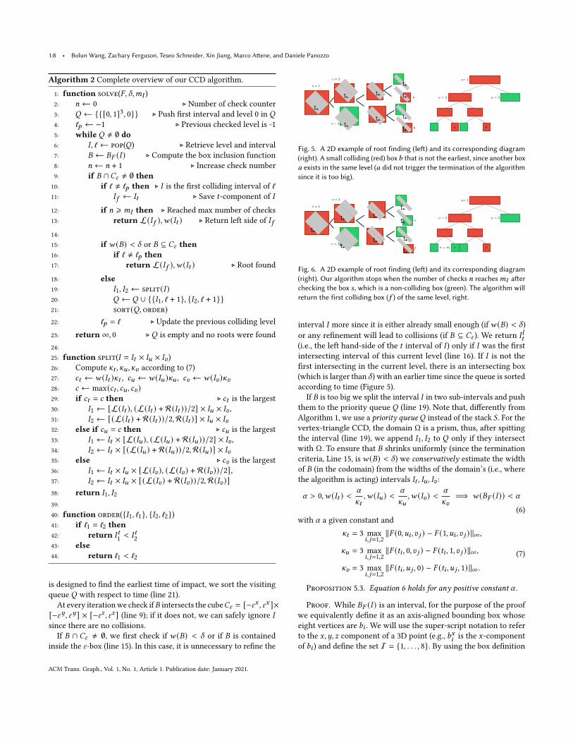
Algorithm. We describe our complete algorithm in pseudocodein Algorithm 2. The input to our algorithm are the eight pointsrepresenting two primitives (either vertex-face or edge-edge), a user-controlled numerical tolerance 𝛿 > 0 (if not specified otherwise,in the experiment we use the default value 𝛿 = 10−6), and themaximum number of checks 𝑚𝐼 > 0 (we use the default value𝑚𝐼 = 106). These choice are based on our empirical results (figures 8and 9). The output is a conservative estimate of the earliest time ofimpact or infinity if the two primitives do not collide in the timeintervals coupled with the reached tolerance.Our algorithm iteratively checks the box 𝐵 = 𝐵𝐹 (𝐼 ), with 𝐼 =

𝐼𝑡 × 𝐼𝑢 × 𝐼𝑣 = [𝑡1, 𝑡2] × [𝑢1, 𝑢2] × [𝑣1, 𝑣2] ⊂ 𝐼Ω (initialized with [0, 1]3).To guarantee a uniform box size while allowing early terminationof the algorithm, we explore the space in a breadth-first mannerand record the current explored level ℓ (line 6). Since our algorithm



Algorithm 2 Complete overview of our CCD algorithm.

1: function solve(𝐹, 𝛿,𝑚𝐼 )2: 𝑛 ← 0 ⊲ Number of check counter3: 𝑄 ← {{[0, 1]3, 0}} ⊲ Push first interval and level 0 in 𝑄

4: ℓ𝑝 ← −1 ⊲ Previous checked level is -15: while 𝑄 ≠ ∅ do

6: 𝐼 , ℓ ← pop(𝑄) ⊲ Retrieve level and interval7: 𝐵 ← 𝐵𝐹 (𝐼 ) ⊲ Compute the box inclusion function8: 𝑛 ← 𝑛 + 1 ⊲ Increase check number9: if 𝐵 ∩𝐶𝜀 ≠ ∅ then

10: if ℓ ≠ ℓ𝑝 then ⊲ 𝐼 is the first colliding interval of ℓ11: 𝐼𝑓 ← 𝐼𝑡 ⊲ Save 𝑡-component of 𝐼

12: if 𝑛 ⩾ 𝑚𝐼 then ⊲ Reached max number of checks13: return L(𝐼𝑓 ),𝑤 (𝐼𝑡 ) ⊲ Return left side of 𝐼𝑓

14:

15: if 𝑤 (𝐵) < 𝛿 or 𝐵 ⊆ 𝐶𝜀 then

16: if ℓ ≠ ℓ𝑝 then

17: return L(𝐼𝑓 ),𝑤 (𝐼𝑡 ) ⊲ Root found

18: else

19: 𝐼1, 𝐼2 ← split(𝐼 )

20: 𝑄 ← 𝑄 ∪ {{𝐼1, ℓ + 1}, {𝐼2, ℓ + 1}}21: sort(𝑄, order)

22: ℓ𝑝 = ℓ ⊲ Update the previous colliding level

23: return∞, 0 ⊲ 𝑄 is empty and no roots were found

24:

25: function split(𝐼 = 𝐼𝑡 × 𝐼𝑢 × 𝐼𝑣 )26: Compute 𝜅𝑡 , 𝜅𝑢 , 𝜅𝑣 according to (7)27: 𝑐𝑡 ← 𝑤 (𝐼𝑡 )𝜅𝑡 , 𝑐𝑢 ← 𝑤 (𝐼𝑢 )𝜅𝑢 , 𝑐𝑣 ← 𝑤 (𝐼𝑣)𝜅𝑣28: 𝑐 ← max(𝑐𝑡 , 𝑐𝑢 , 𝑐𝑣)29: if 𝑐𝑡 = 𝑐 then ⊲ 𝑐𝑡 is the largest30: 𝐼1 ← [L(𝐼𝑡 ), (L(𝐼𝑡 ) + R(𝐼𝑡 ))/2] × 𝐼𝑢 × 𝐼𝑣 ,31: 𝐼2 ← [(L(𝐼𝑡 ) + R(𝐼𝑡 ))/2,R(𝐼𝑡 )] × 𝐼𝑢 × 𝐼𝑣32: else if 𝑐𝑢 = 𝑐 then ⊲ 𝑐𝑢 is the largest33: 𝐼1 ← 𝐼𝑡 × [L(𝐼𝑢 ), (L(𝐼𝑢 ) + R(𝐼𝑢 ))/2] × 𝐼𝑣 ,34: 𝐼2 ← 𝐼𝑡 × [(L(𝐼𝑢 ) + R(𝐼𝑢 ))/2,R(𝐼𝑢 )] × 𝐼𝑣35: else ⊲ 𝑐𝑣 is the largest36: 𝐼1 ← 𝐼𝑡 × 𝐼𝑢 × [L(𝐼𝑣), (L(𝐼𝑣) + R(𝐼𝑣))/2],37: 𝐼2 ← 𝐼𝑡 × 𝐼𝑢 × [(L(𝐼𝑣) + R(𝐼𝑣))/2,R(𝐼𝑣)]

38: return 𝐼1, 𝐼2

39:

40: function order({𝐼1, ℓ1}, {𝐼2, ℓ2})41: if ℓ1 = ℓ2 then

42: return 𝐼𝑡1 < 𝐼𝑡243: else

44: return ℓ1 < ℓ2

is designed to find the earliest time of impact, we sort the visitingqueue 𝑄 with respect to time (line 21).

At every iterationwe check if𝐵 intersects the cube𝐶𝜀 = [−𝜀𝑥 , 𝜀𝑥 ]×[−𝜀𝑦, 𝜀𝑦] × [−𝜀𝑧 , 𝜀𝑧] (line 9); if it does not, we can safely ignore 𝐼since there are no collisions.If 𝐵 ∩ 𝐶𝜀 ≠ ∅, we first check if 𝑤 (𝐵) < 𝛿 or if 𝐵 is contained

inside the 𝜀-box (line 15). In this case, it is unnecessary to refine the

n = 1

n = 2

n = 3

a

b

n= 1

n = 2 n = 3

a b

Fig. 5. A 2D example of root finding (left) and its corresponding diagram

(right). A small colliding (red) box𝑏 that is not the earliest, since another box

𝑎 exists in the same level (𝑎 did not trigger the termination of the algorithm

since it is too big).

n = 1

n = 2

n = 3

f

s

n= 1

n = 2 n = 3

s fn = mI

Fig. 6. A 2D example of root finding (left) and its corresponding diagram

(right). Our algorithm stops when the number of checks 𝑛 reaches𝑚𝐼 after

checking the box 𝑠 , which is a non-colliding box (green). The algorithm will

return the first colliding box (𝑓 ) of the same level, right.

interval 𝐼 more since it is either already small enough (if𝑤 (𝐵) < 𝛿)or any refinement will lead to collisions (if 𝐵 ⊆ 𝐶𝜀 ). We return 𝐼 𝑙𝑡(i.e., the left hand-side of the 𝑡 interval of 𝐼 ) only if 𝐼 was the firstintersecting interval of this current level (line 16). If 𝐼 is not thefirst intersecting in the current level, there is an intersecting box(which is larger than 𝛿) with an earlier time since the queue is sortedaccording to time (Figure 5).

If 𝐵 is too big we split the interval 𝐼 in two sub-intervals and pushthem to the priority queue 𝑄 (line 19). Note that, differently fromAlgorithm 1, we use a priority queue𝑄 instead of the stack 𝑆 . For thevertex-triangle CCD, the domain Ω is a prism, thus, after spittingthe interval (line 19), we append 𝐼1, 𝐼2 to 𝑄 only if they intersectwith Ω. To ensure that 𝐵 shrinks uniformly (since the terminationcriteria, Line 15, is𝑤 (𝐵) < 𝛿) we conservatively estimate the widthof 𝐵 (in the codomain) from the widths of the domain’s (i.e., wherethe algorithm is acting) intervals 𝐼𝑡 , 𝐼𝑢 , 𝐼𝑣 :

𝛼 > 0,𝑤 (𝐼𝑡 ) <𝛼

𝜅𝑡,𝑤 (𝐼𝑢 ) <

𝛼

𝜅𝑢,𝑤 (𝐼𝑣) <

𝛼

𝜅𝑣=⇒ 𝑤 (𝐵𝐹 (𝐼 )) < 𝛼

(6)with 𝛼 a given constant and

𝜅𝑡 = 3 max𝑖, 𝑗=1,2

∥𝐹 (0, 𝑢𝑖 , 𝑣 𝑗 ) − 𝐹 (1, 𝑢𝑖 , 𝑣 𝑗 )∥∞,

𝜅𝑢 = 3 max𝑖, 𝑗=1,2

∥𝐹 (𝑡𝑖 , 0, 𝑣 𝑗 ) − 𝐹 (𝑡𝑖 , 1, 𝑣 𝑗 )∥∞,

𝜅𝑣 = 3 max𝑖, 𝑗=1,2

∥𝐹 (𝑡𝑖 , 𝑢 𝑗 , 0) − 𝐹 (𝑡𝑖 , 𝑢 𝑗 , 1)∥∞ .

(7)

Proposition 5.3. Equation 6 holds for any positive constant 𝛼 .

Proof. While 𝐵𝐹 (𝐼 ) is an interval, for the purpose of the proofwe equivalently define it as an axis-aligned bounding box whoseeight vertices are 𝑏𝑖 . We will use the super-script notation to referto the 𝑥,𝑦, 𝑧 component of a 3D point (e.g., 𝑏𝑥𝑖 is the 𝑥-componentof 𝑏𝑖 ) and define the set I = {1, . . . , 8}. By using the box definition



the width of 𝐵𝐹 (𝐼 ) can be written as

𝑤 (𝐵𝐹 (𝐼 )) = ∥𝑏𝑀 − 𝑏𝑚 ∥∞

with

𝑏𝑘𝑀 = max𝑖∈I(𝑏𝑘𝑖 ) and 𝑏𝑘𝑚 = min

𝑖∈I(𝑏𝑘𝑖 ) .

Since 𝐵𝐹 (𝐼 ) is the tightest axis-aligned inclusion function (Proposi-tion 5.1)

𝑏𝑘𝑀 ⩽ max𝑖∈I

𝑣𝑘𝑖 , 𝑏𝑘𝑚 ⩽ min𝑖∈I

𝑣𝑘𝑖 ,

where 𝑣𝑖 = 𝐹 (𝐼𝑗𝑡 , 𝐼

𝑘𝑢 , 𝐼

𝑙𝑣), with 𝑗, 𝑘, 𝑙 ∈ {𝑙, 𝑟 }, thus for any coordinate

𝑘 we bound

𝑏𝑘𝑀 − 𝑏𝑘𝑚 = max

𝑖, 𝑗 ∈I(𝑣𝑘𝑖 − 𝑣

𝑘𝑗 ) ⩽ max

𝑖, 𝑗 ∈I∥𝑣𝑖 − 𝑣 𝑗 ∥∞ .

For any pair of 𝑣𝑖 and 𝑣 𝑗 we have

𝑣𝑖 − 𝑣 𝑗 = 𝑠1𝛼𝑙,𝑚 + 𝑠2𝛽𝑛,𝑝 + 𝑠3𝛾𝑝,𝑞,

for some indices 𝑙,𝑚, 𝑛, 𝑜, 𝑝, 𝑞 ∈ {1, 2} and constant 𝑠1, 𝑠2, 𝑠3 ∈{−1, 0, 1} with

𝛼𝑖, 𝑗 = 𝑤 (𝐼𝑡 )(

𝐹 (0, 𝑢𝑖 , 𝑣 𝑗 ) − 𝐹 (1, 𝑢𝑖 , 𝑣 𝑗 ))

,

𝛽𝑖, 𝑗 = 𝑤 (𝐼𝑢 )(

𝐹 (𝑡𝑖 , 0, 𝑣 𝑗 ) − 𝐹 (𝑡𝑖 , 1, 𝑣 𝑗 ))

,

𝛾𝑖, 𝑗 = 𝑤 (𝐼𝑣)(

𝐹 (𝑡𝑖 , 𝑢 𝑗 , 0) − 𝐹 (𝑡𝑖 , 𝑢 𝑗 , 1))

,

since 𝐹 is linear on the edges. We note that 𝛼𝑖, 𝑗 , 𝛽𝑖, 𝑗 , and 𝛾𝑖, 𝑗 are the12 edges of the box 𝐵𝐹 . We now define

𝑒𝑘𝑡 = max𝑖, 𝑗 ∈{1,2}

|𝛼𝑘𝑖,𝑗 |, 𝑒𝑘𝑢 = max𝑖, 𝑗 ∈{1,2}

|𝛽𝑘𝑖,𝑗 |, 𝑒𝑘𝑣 = max𝑖, 𝑗 ∈{1,2}

|𝛾𝑘𝑖,𝑗 |

which allows us to bound

max𝑖, 𝑗 ∈I

∥𝑣𝑖 − 𝑣 𝑗 ∥∞ ⩽ ∥𝑒𝑡 + 𝑒𝑢 + 𝑒𝑣 ∥∞ ⩽ ∥𝑒𝑡 ∥∞ + ∥𝑒𝑢 ∥∞ + ∥𝑒𝑣 ∥∞ .

Since

∥𝑒𝑡 ∥∞ ⩽ 𝑤 (𝐼𝑡 ) max𝑖, 𝑗=1,2

∥𝐹 (𝑡1, 𝑢𝑖 , 𝑣 𝑗 ) − 𝐹 (𝑡2, 𝑢𝑖 , 𝑣 𝑗 )∥∞ = 𝑤 (𝐼𝑡 )𝜅𝑡/3,

and similarly ∥𝑒𝑢 ∥∞ ⩽ 𝜅𝑢/3, ∥𝑒𝑣 ∥∞ ⩽ 𝜅𝑣/3, we have

∥𝑒𝑡 ∥∞ + ∥𝑒𝑢 ∥∞ + ∥𝑒𝑣 ∥∞ ⩽𝑤 (𝐼𝑡 )𝜅𝑡 +𝑤 (𝐼𝑢 )𝜅𝑢 +𝑤 (𝐼𝑣)𝜅𝑣

3

Finally, from the assumption (6) it follows that

𝑤 (𝐵𝐹 (𝐼 )) ⩽ max𝑖, 𝑗 ∈I

∥𝑣𝑖 − 𝑣 𝑗 ∥∞ ⩽ ∥𝑒𝑡 ∥∞ + ∥𝑒𝑢 ∥∞ + ∥𝑒𝑣 ∥∞ < 𝛼.

□

Using the estimate of the width of 𝐼𝑡 , 𝐼𝑢 , 𝐼𝑣 we split the dimensionthat leads to the largest estimated dimension in the range of 𝐹(line 28).

Fixed Runtime or Fixed Accuracy. To ensure a bounded runtime,which is very useful in many simulation applications, we stop thealgorithm after an user-controlled number of checks𝑚𝐼 . To ensurethat our algorithm always returns a conservative time of impact werecord the first colliding interval 𝐼𝑓 of every level (line 11). Whenthe maximum number of check is reached we can safely returnthe latest recorded interval 𝐼𝑓 (line 13) (Figure 6). We note thatour algorithm will not respect the user specified accuracy when itterminates early: if a constant accuracy is required by applications,this additional termination criteria could be disabled, obtaining analgorithmwith guaranteed accuracy but sacrificing the bound on themaximal running time. Note that without the termination criteria𝑚𝐼 , it is possible (while rare in our experiments) that the algorithmwill take a long time to terminate, or run out of memory due tostoring the potentially large list of candidate intervals 𝐿.

5.3 Results

Our algorithm is implemented in C++ and uses Eigen [Guennebaudet al. 2010] for the linear algebra routines (with the -avx2 g++ flag).We run our experiments on a 2.35 GHz AMDEPYC™ 7452.We attachthe reference implementation and the data used for our experiments,which will be released publicly.

The running time of our method is comparable to the floating-point methods, while being provably correct, for any choice ofparameters. For this comparison we use a default tolerance 𝛿 =

10−6 and default number of iterations 𝑚𝐼 = 106. All queries inthe simulation dataset terminate within 106 checks, while for thehandcrafted dataset only 0.25% and 0.55% of the vertex-face andedge-edge queries required more than 106 checks, reaching an actualmaximal tolerance 𝛿 of 2.14 × 10−5 and 6.41 × 10−5 for vertex-faceand edge-edge respectively. We note that, despite the percentagesbegin small, by removing𝑚𝐼 the handcrafted queries take 0.015774and 0.042477 seconds on average for vertex-face and edge-edgerespectively. This is due to the large number of degenerate queries,as can be seen from the long tail in the histogram of the run-times(Figure 7). We did not observe any noticeable change of runningtime for the simulation dataset.

Our algorithm has two user-controlled parameters (𝛿 and𝑚𝐼 ) tocontrol the accuracy and running time. The tolerance 𝛿 providesa direct control on the achieved accuracy and provides an indirecteffect on the running time (Figure 8). The other parameter, 𝑚𝐼 ,directly controls the maximal running time of each query: for small𝑚𝐼 our algorithmwill terminate earlier, resulting in a lower accuracyand thus more chances of false positives (Figure 9 top). We remarkthat, in practice, very few queries require so many subdivisions:by reducing𝑚𝐼 to the very low value of 100, our algorithm early-terminates only on∼0.07% of the 60million queries in the simulationdataset.

6 MINIMUM SEPARATION CCD

An additional feature of some CCD algorithms isminimal separation,that is, the option to report collision at a controlled distance froman object, which is used to ensure that objects are never too close.This is useful to avoid possible inter-penetrations introduced bynumerical rounding after the collision response, or for modeling



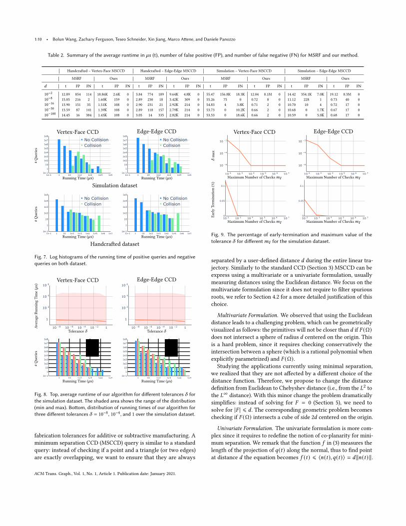
Table 2. Summary of the average runtime in 𝜇𝑠 (t), number of false positive (FP), and number of false negative (FN) for MSRF and our method.

Handcrafted ś Vertex-Face MSCCD Handcrafted ś Edge-Edge MSCCD Simulation ś Vertex-Face MSCCD Simulation ś Edge-Edge MSCCD

MSRF Ours MSRF Ours MSRF Ours MSRF Ours

𝑑 t FP FN t FP FN t FP FN t FP FN t FP FN t FP FN t FP FN t FP FN

10−2 12.89 854 114 18.86K 2.6K 0 3.84 774 189 9.64K 4.8K 0 55.47 156.8K 18.3K 12.04 8.1M 0 14.42 354.1K 7.0K 19.12 8.3M 010−8 15.05 216 2 1.60K 159 0 2.89 230 18 3.42K 309 0 55.26 75 0 0.72 8 0 11.12 228 1 0.73 40 010−16 13.90 151 35 1.51K 108 0 2.90 231 21 2.92K 214 0 54.83 4 3.8K 0.71 2 0 10.70 10 4 0.72 17 010−30 13.59 87 141 1.39K 108 0 2.89 118 157 2.79K 214 0 53.73 0 10.2K 0.66 2 0 10.68 0 1.7K 0.67 17 010−100 14.45 16 384 1.43K 108 0 3.05 14 335 2.82K 214 0 53.53 0 18.6K 0.66 2 0 10.59 0 5.0K 0.68 17 0

Vertex-Face CCD Edge-Edge CCD

#Queries

1e-1 1 10 1e2 1e3 1e4 1e51e-1

1

10

1e2

1e3

1e4

1e5

1e6

1e7

1e8

No Collision

Collision

1e-1 1 10 1e2 1e3 1e4 1e51e-1

1

10

1e2

1e3

1e4

1e5

1e6

1e7

1e8

No Collision

Collision

Running Time (𝜇𝑠) Running Time (𝜇𝑠)

Simulation dataset

#Queries

1e-1 1 10 1e2 1e3 1e4 1e5 1e6 1e71e-1

1

10

1e2

1e3

1e4

1e5

No Collision

Collision

1e-1 1 10 1e2 1e3 1e4 1e5 1e6 1e71e-1

1

10

1e2

1e3

1e4

1e5

No Collision

Collision

Running Time (𝜇𝑠) Running Time (𝜇𝑠)

Handcrafted dataset

Fig. 7. Log histograms of the running time of positive queries and negative

queries on both dataset.


Average

RunningTim

e(𝜇s)

10 −8

10 −6

10 −4

10 −2

1

1

10 2

10 4

10 6

10 −8

10 −6

10 −4

10 −2

1

1

10 2

10 4

10 6

Tolerance 𝛿 Tolerance 𝛿

#Queries

1 10 1e2 1e3 1e4 1e51e-1

1

10

1e2

1e3

1e4

1e5

1e6

1e7

1e8 δ =1δ =10-4δ =10-8

1 10 1e2 1e3 1e4 1e51e-1

1

10

1e2

1e3

1e4

1e5

1e6

1e7

1e8 δ =1δ =10-4δ =10-8

Running Time (𝜇s) Running Time (𝜇s)

Fig. 8. Top, average runtime of our algorithm for different tolerances 𝛿 for

the simulation dataset. The shaded area shows the range of the distribution

(min and max). Bottom, distribution of running times of our algorithm for

three different tolerances 𝛿 = 10−8, 10−4, and 1 over the simulation dataset.

fabrication tolerances for additive or subtractive manufacturing. Aminimum separation CCD (MSCCD) query is similar to a standardquery: instead of checking if a point and a triangle (or two edges)are exactly overlapping, we want to ensure that they are always


𝛿max

10 2 10

3 10

4 10

5 10

6 10

7

10 −6

10 −4

10 −2

10 2 10

3 10

4 10

5 10

6 10

7

10 −6

10 −4

10 −2

Maximum Number of Checks𝑚𝐼 Maximum Number of Checks𝑚𝐼

Early

Termination(%)

10 2 10

3 10

4 10

5 10

6 10

7

0

0.05

0.1

10 2 10

3 10

4 10

5 10

6 10

7

0

0.05

0.1

Maximum Number of Checks𝑚𝐼 Maximum Number of Checks𝑚𝐼

Fig. 9. The percentage of early-termination and maximum value of the

tolerance 𝛿 for different𝑚𝐼 for the simulation dataset.

separated by a user-defined distance 𝑑 during the entire linear tra-jectory. Similarly to the standard CCD (Section 3) MSCCD can beexpress using a multivariate or a univariate formulation, usuallymeasuring distances using the Euclidean distance. We focus on themultivariate formulation since it does not require to filter spuriousroots, we refer to Section 4.2 for a more detailed justification of thischoice.

Multivariate Formulation. We observed that using the Euclideandistance leads to a challenging problem, which can be geometricallyvisualized as follows: the primitives will not be closer than 𝑑 if 𝐹 (Ω)does not intersect a sphere of radius 𝑑 centered on the origin. Thisis a hard problem, since it requires checking conservatively theintersection between a sphere (which is a rational polynomial whenexplicitly parametrized) and 𝐹 (Ω).Studying the applications currently using minimal separation,

we realized that they are not affected by a different choice of thedistance function. Therefore, we propose to change the distancedefinition from Euclidean to Chebyshev distance (i.e., from the 𝐿2 tothe 𝐿∞ distance). With this minor change the problem dramaticallysimplifies: instead of solving for 𝐹 = 0 (Section 5), we need tosolve for |𝐹 | ⩽ 𝑑 . The corresponding geometric problem becomeschecking if 𝐹 (Ω) intersects a cube of side 2𝑑 centered on the origin.

Univariate Formulation. The univariate formulation is more com-plex since it requires to redefine the notion of co-planarity for mini-mum separation. We remark that the function 𝑓 in (3) measures thelength of the projection of 𝑞(𝑡) along the normal, thus to find pointat distance 𝑑 the equation becomes 𝑓 (𝑡) ⩽ ⟨𝑛(𝑡), 𝑞(𝑡)⟩ = 𝑑 ∥𝑛(𝑡)∥.



0 1

Ig

g

Cd

-d

0 1

I0

0 1

Ig

g

Cd

-d

0.50

I1 I2

0.5

1

0 1

Ig

g

Cd

-d

0.5

0.25

I3 I4

0.5

0.250

ℓ = 0 ℓ = 1 ℓ = 2

Fig. 10. 1D illustration of the first three levels of our MSCCD inclusion

based root-finder. Instead of checking if 𝐼𝑔 intersects with the origin, we

check if it intersects the interval [−𝑑,𝑑 ] marked in light green.

To keep the equation polynomial, remove the inequality, and avoidsquare roots, the univariate MSCCD root finder becomes

⟨𝑛(𝑡), 𝑞(𝑡)⟩2 − 𝑑2∥𝑛(𝑡)∥2 .

We note that this polynomial becomes sextic, and not cubic as inthe zero-distance version. To account for replacing the inequalitywith an equality, we also need to check for distance between 𝑞

and the edges and vertices of the triangle [Harmon et al. 2011]. Inaddition to finding the roots of several high-order polynomials, thisformulation, similarly to the standard CCD, suffers from infiniteroots when the two primitives are moving on a plane at distance 𝑑from each other.

6.1 Method

The input to our MSCCD algorithm are the same as the standardCCD (eight coordinates, 𝛿 , and𝑚𝐼 ) and the minimum separationdistance 𝑑 ⩾ 0. Our algorithm returns the earliest time of impactindicating if two primitives become closer than 𝑑 as measured bythe 𝐿∞ norm.We wish to check whether the box 𝐵𝐹 (Ω) intersects a cube of

side 2𝑑 centered on the origin (Figure 10). Equivalently, we canconstruct another box 𝐵′

𝐹(Ω) by displacing the six faces of 𝐵𝐹 (Ω)

outward at a distance 𝑑 , and then check whether this enlarged boxcontains the origin. This check can be done as for the standard CCD(Section 5), but the floating point filters must be recalculated toaccount for the additional sum (indeed, we add/subtract 𝑑 to/fromall the coordinates). Hence, the filters for 𝐹 ′ are:

𝜖𝑥ee = 7.105427357601002 × 10−15𝛾3𝑥𝜖𝑥vf = 7.549516567451064 × 10−15𝛾3𝑥

(8)

As before, the filters are calculated as described in [Attene 2020]and they additionally assume that 𝑑 < 𝛾𝑥 .To account for minimum separations, the only change in our

algorithm is at line 7 where we need to enlarge 𝐵 by 𝑑 and inlines 9 and 15 since 𝐶𝜀 needs to be replaced with 𝐶𝜖 = [−𝜖𝑥 , 𝜖𝑥 ] ×

[−𝜖𝑦, 𝜖𝑦] × [−𝜖𝑧 , 𝜖𝑧].

6.2 Results

To the best of our knowledge, the minimum separation floating-point time-of-impact root finder [Harmon et al. 2011] (MSRF) im-plemented in [Lu et al. 2019], is the only public code supportingminimal separation queries. While not explicitly constructed for

Vertex-Face MSCCD Edge-Edge MSCCD

Average

RunningTim

e(𝜇s)

10 −84

10 −63

10 −42

10 −21

1

1

10 2

10 4

10 6

10 −84

10 −63

10 −42

10 −21

1

1

10 2

10 4

10 6

Distance 𝑑 Distance 𝑑

#Queries

1 10 1e2 1e3 1e4 1e51e-1

1

10

1e2

1e3

1e4

1e5

1e6

1e7

1e8

d =1

d =10-8

d =10-50

1 10 1e2 1e3 1e4 1e51e-1

1

10

1e2

1e3

1e4

1e5

1e6

1e7

1e8

d =1

d =10-8

d =10-50

Running Time (𝜇s) Running Time (𝜇s)

Fig. 11. Top, average runtime of our algorithm for varying minimum sepa-

ration 𝑑 in the simulation dataset. The shaded area depicts the range of the

values. Bottom, distribution of running time for three different minimum

separation distanced 𝑑 = 10−50, 10−8, and 1 over the simulation dataset.

MSCCD, FPRF uses a distance tolerance to limit false negatives, sim-ilarly to an explicit minimum separation. We compare the resultsand performance in Appendix E.

MSRF. uses the univariate formulation, which requires to findthe roots of a high-order polynomial, and it is thus unstable whenimplemented using floating-point arithmetic.Table 2 reports timings, false positive, and false negatives for

different separation distances 𝑑 . As 𝑑 shrinks (around 10−16) theresults of our method with MSCDD coincide with the ones with𝑑 = 0 since the separation is small. For these small tolerances, MSRFruns into numerical problems and the number of false negativesincreases. Figure 11 shows the average query time versus the sepa-ration distance 𝑑 for the simulation dataset, since our method onlyrequires to check the intersection between boxes, the running timelargely depends on the number of detected collision, and the averageis only mildly affected by the choice of 𝑑 .

7 INTEGRATION IN EXISTING SIMULATORS

In a typical simulation the objects are represented using triangularmeshes and the vertices are moving along a linear trajectory in atimestep. At each timestep, collisions might happen when a vertexhits a triangle, or when an edge hits another edge. A CCD algorithmis then used to prevent interpenetration; this can be done in differentways. In an active set construction method (Section 7.1) the CCDis used to compute contact forces to avoid penetration assuminglinearized contact behaviour. For a line-search based method (Sec-tion 7.2), CCD and time of impact are used to prevent the Newtontrajectory from causing penetration by limiting the step length. Notethat, the latter approach requires a conservative CCD, while theformer can tolerate false negatives.The integration of a CCD algorithm with collision response al-

gorithms is a challenging problem on its own, which is beyond thescope of this paper. As a preliminary study, to show that our method



can be integrated in existing response algorithm, we examine twouse cases in elastodynamic simulations:

(1) constructing an active set of collision constraints [Harmonet al. 2008; Verschoor and Jalba 2019; Wriggers 1995], Sec-tion 7.1;

(2) during a line search to prevent intersections [Li et al. 2020],Section 7.2.

We leave as future work a more comprehensive study includinghow to use our CCD to further improve the physical fidelity ofexisting simulators or how to deal with challenging cases such assliding contact response.To keep consistency across queries, we compute the numerical

tolerances (5) and (8) for the whole scene. That is, 𝑥max, 𝑦max, and𝑧max are computed as the maximum over all the vertices in thesimulation. In algorithms 3 and 4 we utilize a broad phase method(e.g., spatial hash) to reduce the number of candidates 𝐶 that needto be evaluated with out narrow phase CCD algorithm.

7.1 Active Set Construction

Algorithm 3 Active Set Construction Using Exact CCD

1: function ConstructActiveSet(𝑥0, 𝑥1, 𝛿,𝑚𝐼 )2: 𝐶 ← BroadPhase(𝑥0, 𝑥1)3: 𝐶𝐴 ← ∅

4: for 𝑐 ∈ 𝐶 do ⊲ Iterate over the collision candidates5: 𝑡 ← CCD(𝑥0 ∩ 𝑐, 𝑥1 ∩ 𝑐, 𝛿,𝑚𝐼 )6: if 0 ⩽ 𝑡 ⩽ 1 then7: 𝐶𝐴 ← 𝐶𝐴 ∪ {(𝑐, 𝑡)}

8: return 𝐶𝐴

9:

10: function CCD(𝑐0, 𝑐1, 𝛿,𝑚𝐼 )11: if 𝑐0 and 𝑐1 are edges then12: 𝐹 ← build 𝐹ee from 𝑐0 and 𝑐1 ⊲ Equation (2)13: else

14: 𝐹 ← build 𝐹vf from 𝑐0 and 𝑐1 ⊲ Equation (1)

15: return Solve(𝐹, 𝛿,𝑚𝐼 )

In the traditional constraint based collision handling (such as thatof Verschoor and Jalba [2019]), collision response is handled by per-forming an implicit timestep as a constrained optimization. The goalis to minimize a elastic potential while avoiding interpenetrationthrough gap constraints. To avoid handling all possible collisionsduring a simulation, a subset of active collisions constraints 𝐶𝐴 isusually constructed. This set not only avoids infeasibilities, but alsoimproves performance by having fewer constraints. There are manyactivation strategies, but for the sake of brevity we focus here onthe strategies used by Verschoor and Jalba [2019].Algorithm 3 shows how CCD is used to compute the active set

𝐶𝐴 . Given the starting and ending vertex positions, 𝑥0 and 𝑥1, wecompute the time of impact for each collision candidate 𝑐 ∈ 𝐶 . Weuse the notation 𝑥𝑖 ∩ 𝑐 to indicate selecting the constrained verticesfrom 𝑥𝑖 . If the candidate 𝑐 is an actual collision, that is 0 ⩽ 𝑡 ⩽ 1,then we add this constraint and the time of impact, 𝑡 , to the activeset, 𝐶𝐴 .

𝛿 = 10−1 𝛿 = 10−3 𝛿 = 10−6

Fig. 12. An elastic simulation using the constraints and active set method

of Verschoor and Jalba [2019]. From an initial configuration (left) we simulate

an elastic torus falling on a fixed cone using three values of 𝛿 (from left

to right: 10−1, 10−3, 10−6). The total runtime of the simulation is affected

little by the change in 𝛿 (24.7, 25.2, and 26.2 seconds from left to right

compared to 32.3 seconds when using FPRF). For 𝛿 = 10−1, inaccuracies inthe time-of-impact lead to inaccurate contact points in the constraints and,

ultimately, intersections (inset).

From the active constraint set the constraints of Verschoor andJalba [2019] are computed as

⟨𝑛, 𝑝1𝑐 − 𝑝2𝑐 ⟩ ⩾ 0,

where 𝑛 is the contact normal (i.e., for a point-triangle the trianglenormal at the time of impact and for edge-edge the edge-edge crossproduct at the time of impact), 𝑝1𝑐 is the point (or the contact pointon the first edge), and 𝑝2𝑐 is the point of contact on the triangle(or on the second edge) at the end of the timestep. Note that, thisconstraint requires to compute the point of contact, which dependson the the time-of-impact which can be obtained directly from ourmethod.Because of the difficulty for a simulation solver to maintain and

not violate constraints, it is common to offset the constraints suchthat

⟨𝑛, 𝑝1𝑐 − 𝑝2𝑐 ⟩ ⩾ 𝜂 > 0.

In such a way, even if the 𝜂 constraint is violated, the real constraintis still satisfied. This common trick, implies that the constraints needto be activated early (i.e., when the distance between two objectsis smaller than 𝜂) which is exactly what our MSCCD can computewhen using 𝑑 = 𝜂. In Figure 12, we use a value of 𝜂 = 0.001m. Whenusing large values of 𝜂, the constraint of Verschoor and Jalba [2019]can lead to infeasibilities because all triangles are extended to planesand edges to lines.Figure 12 shows example of simulations run with different nu-

merical tolerance 𝛿 . Changing 𝛿 has little effect on the simulationin terms of run-time, but for large values of 𝛿 , it can affect accuracy.We observe that for a 𝛿 ⩾ 10−2 the simulation is more likely tocontain intersections. This is most likely due to the inaccuracies inthe contact points used in the constraints.

7.2 Line Search

A line search is used in a optimization to ensure that every up-date decreases the energy 𝐸. That is, given an update, Δ𝑥 , to theoptimization variable 𝑥 , we want to find a step size 𝛼 such that𝐸 (𝑥 + 𝛼Δ𝑥) < 𝐸 (𝑥). This ensure that we make progress towards aminimum.



Algorithm 4 Line Search with Exact CCD

1: function LineSearch(𝐸, 𝑥0,Δ𝑥, 𝑝, 𝛿,𝑚𝐼 )2: 𝑥1 ← 𝑥0 + Δ𝑥

3: 𝐶 ← BroadPhase(𝑥0, 𝑥1) ⊲ Collision candidates4: 𝛼 ← 15: 𝑑𝑖 , 𝜌𝑖 ← Distance(𝐶)

6: Compute 𝜖𝑖 from (8)7: 𝑑 ← max(𝑝𝑑𝑖 , 𝛿)8: while 𝑝 < (𝑑 − 𝛿 − 𝜖𝑖 − 𝜌𝑖 )/𝑑 do

9: 𝑝 ← 𝑝/210: 𝑑 ← 𝑝𝑑𝑖

11: 𝛿𝑖 ← 𝛿

12: for 𝑐 ∈ 𝐶 do ⊲ 𝛼 is bounded by earliest time-of-impact13: 𝑡, 𝛿𝑖 ←MSCCD(𝑥0 ∩ 𝑐, 𝑥1 ∩ 𝑐, 𝑑, 𝛼, 𝛿,𝑚𝐼 )14: 𝛼 ← min(𝑡, 𝛼)15: 𝛿𝑖 ← max(𝛿𝑖 , 𝛿𝑖 )

16: if 𝑝 < (𝑑 − 𝛿𝑖 − 𝜖𝑖 − 𝜌𝑖 )/𝑑 then

17: 𝛿 ← 𝛿𝑖 ⊲ Repeat with 𝑝 validated from 𝛿𝑖18: Go to line 8.19:

20: while 𝛼 > 𝛼min do ⊲ Backtracking line-search21: 𝑥1 ← 𝑥0 + 𝛼Δ𝑥

22: if 𝐸 (𝑥1) < 𝐸 (𝑥0) then ⊲ Objective energy decrease23: break

24: 𝛼 ← 𝛼/2

25: return 𝛼

26:

27: functionMSCCD(𝑐0, 𝑐1, 𝑑, 𝑡, 𝛿,𝑚𝐼 )28: if 𝑐0 and 𝑐1 are edges then29: 𝐹 ← build 𝐹ee from 𝑐0 and 𝑐1 ⊲ Equation (2)30: else

31: 𝐹 ← build 𝐹vf from 𝑐0 and 𝑐1 ⊲ Equation (1)

32: return SolveMSCCD(𝐹, 𝑡, 𝛿,𝑚𝐼 , 𝑑)

When used in a line search algorithm, CCD can be used to preventintersections and tunneling. This requires modifying the maximumstep length to the time of impact. As observed by Li et al. [2020],the standard CCD formulation without minimal separation cannotbe used directly in a line search algorithm. Let 𝑡★ the earliest timeof impact (i.e., 𝐹 (𝑡★, �̃�, 𝑣) = 0 for some �̃�, 𝑣 and there is no collisionbetween 0 and 𝑡★) and assume that the energy at 𝐸 (𝑥0 + 𝑡★Δ𝑥) <𝐸 (𝑥0) (Algorithm 4, line 22). In this case the step 𝛼 = 𝑡★ is a validdescent step which will be used to update the position 𝑥 in outeriteration (e.g., Newton optimization loop). In the next iteration, theline search will be called with the updated position and the earliesttime of impact will be zero since we selected 𝑡★ in the previousiteration. This prevents the optimization from making progressbecause any direction Δ𝑥 will lead to a time of impact 𝑡 = 0. Toavoid this problem we need the line search to find an appropriatestep-size 𝛼 along the update direction that leaves łsufficient spacežfor the next iteration, so that the barrier in [Li et al. 2020] will beactive and steer the optimization away from the contact position.

Formally, we aim at finding a valid CCD sequence {𝑡𝑖 } such that

𝑡𝑖 < 𝑡𝑖+1, lim𝑖→∞

𝑡𝑖 = 𝑡★, and 𝑡𝑖/𝑡𝑖+1 ≈ 1.

The first requirement ensures that successive CCD checkswill reportan increasing time, the second one ensures that we will convergeto the true minimum, and the last one aims at having a łslowlyžconvergent sequence (necessary for numerical stability). Li et al.[2020] exploit a feature of FPRF to simulate a minimal separationCCD: in this work we propose to directly use our MSCCD algorithm(Section 6).

Constructing a Sequence. Let 0 < 𝑝 < 1 be a user-defined tolerance(𝑝 close to 1 will produce a sequence {𝑡𝑖 } converging faster) and 𝑑𝑖be the distance between two primitives. We propose to set 𝑑 = 𝑝𝑑𝑖 ,and ensure that no primitive are closer than 𝑑 . Without loss ofgenerality, we assume that 𝐹 (𝑥 +Δ𝑥) = 0, that is, taking the full stepwill lead to contact. By taking successive steps in the same direction,𝑑𝑖 will shrink to zero ensuring 𝑡𝑖 to converge to 𝑡★. Similarly wewill obtain a growing sequence 𝑡𝑖 since 𝑑 decreases as we proceedwith the iterations. Finally, it is easy to see that 𝑝 = 𝑡𝑖/𝑡𝑖+1 whichcan be close to one.

To account for the aforementioned problem, we propose to use ourMSCCD algorithm to return a valid CCD sequence when employedin a line search scenario. For a step 𝑖 , we define 𝛿𝑖 as the tolerance,𝜖𝑖 the numerical error (8), and 𝜌𝑖 as the maximum numerical errorin computing the distances 𝑑𝑖 from the candidates set 𝐶 (line 5). 𝜌𝑖should be computed using forward error analysis on the application-specific distance computation: since the applications are not thefocus of our paper, we used a fixed 𝜌𝑖 = 10−9, and we leave thecomplete forward analysis as a future work. (We note that ourapproximation might thus introduce zero length steps, this howeverdid not happen in our experiments.) If 𝑑𝑖 − (𝛿𝑖 + 𝜖𝑖 + 𝜌𝑖 ) > 𝑑 , ourMSCCD is guaranteed to find a time of impact larger than zero. Thusif we set 𝑑 = 𝑝𝑑𝑖 (line 7), we are guaranteed to find a positive timeof impact if

𝑑𝑖 >𝛿𝑖 + 𝜖𝑖 + 𝜌𝑖

1 − 𝑝.

To ensure that this inequality holds, we propose to validate 𝑝 beforeusing the MSCCD with 𝛿 (line 8), find the time of impact and theactual 𝛿𝑖 (line 12), and check if the used 𝑝 is valid (line 16). In case𝑝 is too large, we divide it by two until it is small enough. Note that,it might be that

𝑑𝑖 < 𝛿𝑖 + 𝜖𝑖 + 𝜌𝑖 ,

in this case we can still enforce the inequality by increasing thenumber of iterations, decreasing 𝛿 , or using multi-precision in theMSCCD to reduce 𝜖𝑖 . However, this was never necessary in any ofour queries, and we thus leave a proper study of these options as afuture work.As visible from Table 2, our MSCCD slows down as 𝑑 grows.

Since the actual minimum distance is not relevant in the line searchalgorithm, our experiments suggest to cap it at 𝛿 (line 7). To avoidunnecessary computations and speedup the MSCCD computations,our algorithm, as suggested by Redon et al. [2002], can be easilymodified to accept a shorter time interval (line 13): it only requiresto change the initialization of 𝐼 (Algorithm 2 line 3). These twomodifications lead to a 8× speedup in our experiments. We refer



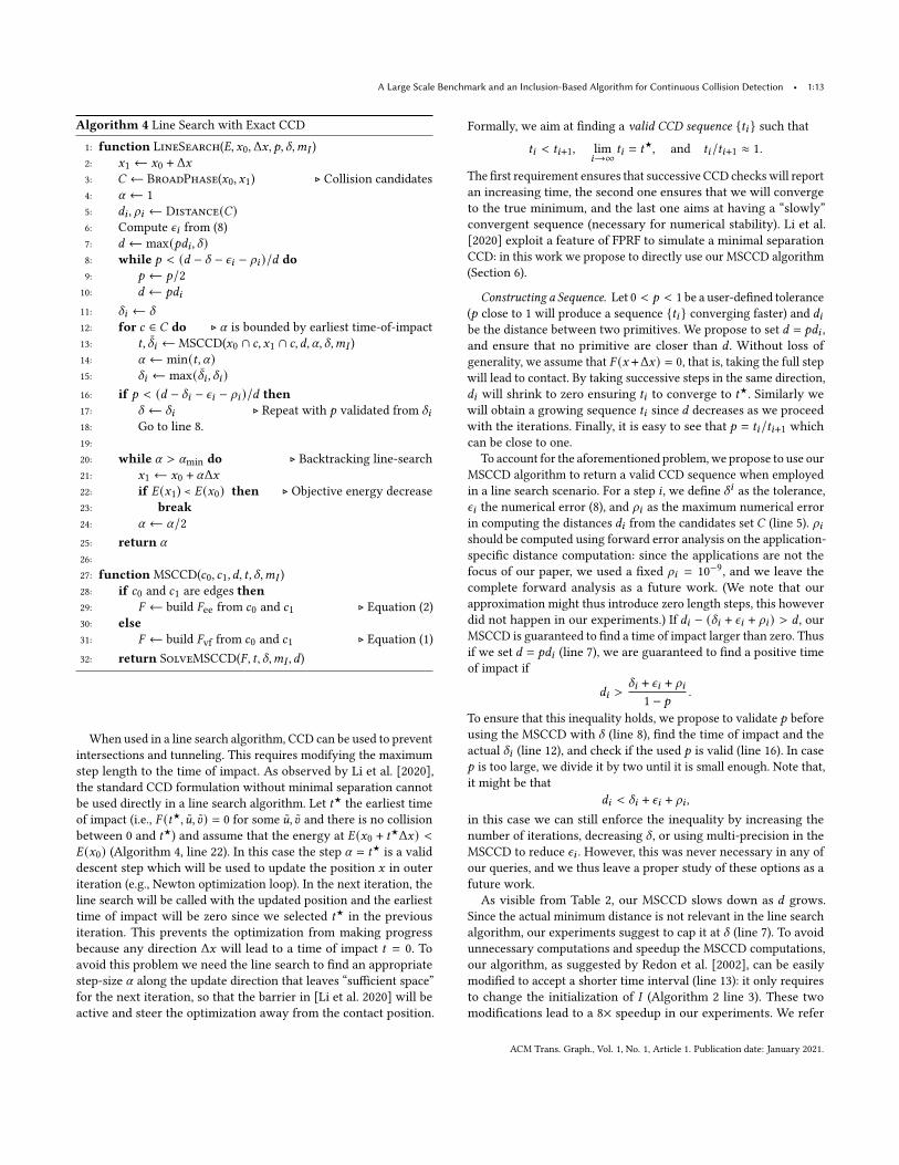
𝛿 = 10−3 𝛿 = 10−4.5 𝛿 = 10−6

Fig. 13. An example of an elastic simulation using our line search (Sec-

tion 7.2) and the method of Li et al. [2020] to keep the bodies from intersect-

ing. An octocat is falling under gravity onto a triangulated plane. From left

to right: the initial configuration, the final frame with 𝛿 = 10−3, 𝛿 = 10−4.5,𝛿 = 10−6 all with a maximum of 106 iterations. There are no noticeable

differences in the results, and the entire simulations takes 63.3, 67.9, and67.0 seconds from left to right (a speed up compared to using FPRF which

takes 102 seconds). ©Brian Enigma under CC BY-SA 3.0.

to this algorithm with MSCCD (i.e., Algorithm 2 with MSCDD,Section 6.1, and modified initialization of 𝐼 ) as SolveMSCCD.

Figure 13 shows a simulation using our MSCCD in line search tokeep the bodies from intersecting for different 𝛿 . As illustrated inthe previous section, the effect of 𝛿 is negligible as long as 𝛿 ⩽ 10−3.Timings vary depending on the maximum number of iterations.Because the distance 𝑑 varies throughout the simulation, some stepstake longer than others (as seen in Figure 11). We note that, if we usethe standard CCD formulation 𝐹 = 0, the line search gets stuck in allour experiments, and we were not able to find a solution. Note thatfor a line search based method it is crucial to have a conservativeCCD/MSCCD algorithm: the videos in the additional material showsthat a false negative leads to an artefact in the simulation.

8 LIMITATIONS AND CONCLUDING REMARKS

We constructed a benchmark of CCD queries and used it to studythe properties of existing CCD algorithms. The study highlightedthat the multivariate formulation is more amenable to robust im-plementations, as it avoids a challenging filtering of spurious roots.This formulation, paired with an interval root finder and modernpredicate construction techniques leads to a novel simple, robust,and efficient algorithm, supporting minimal separation queries withruntime comparable to state of the art, non conservative, methods.While we believe that it is practically acceptable, our algorithm

still suffers from false positive and it will be interesting to see ifthe multivariate root finding could be done exactly with reasonableperformances, for example employing expansion arithmetic in thepredicates. Our definition of minimal separation distance is slightlydifferent from the classical definition, and it would be interestingto study how to extend out method to directly support Euclideandistances. Another interesting venue for future work is the extensionof our inclusion function to non-linear trajectories and their efficientevaluation using static filters or exact arithmetic.Our benchmark focuses only on CPU implementations: reim-

plementing our algorithm on a GPU with our current guaranteesis a major challenge. It will require to control the floating-pointrounding on the GPU (and compliant with the IEEE floating-pointstandard), to ensure that the compiler does not reorder the opera-tions or skip the computation of temporaries. Additionally it wouldrequire to recompute the ground truth and the numerical constantsfor single precision arithmetic, as most GPUs do not yet support

double computation. This is an exciting direction for future work tofurther improve the performance of our approach.

We will release an open-source reference implementation of ourtechnique with anMIT license to foster adoption of our technique byexisting commercial and academic simulators. We will also releasethe dataset and the code for all the algorithms in our benchmark toallow researchers working on CCD to easily compare the perfor-mance and correctness of future CCD algorithms.

ACKNOWLEDGMENTS

We thank Danny Kaufman for valuable discussions and NYU ITHigh Performance Computing for resources, services, and staff ex-pertise. This work was partially supported by the NSF CAREERaward under Grant No. 1652515, the NSF grants OAC-1835712, OIA-1937043, CHS-1908767, CHS-1901091, National Key Research andDevelopment Program of China No. 2020YFA0713700, EU ERC Ad-vanced Grant CHANGE No. 694515, a Sloan Fellowship, a gift fromAdobe Research, a gift from nTopology, and a gift from AdvancedMicro Devices, Inc.

REFERENCESMarco Attene. 2020. Indirect Predicates for Geometric Constructions. Computer-Aided

Design 126 (2020).Tyson Brochu, Essex Edwards, and Robert Bridson. 2012. Efficient Geometrically Exact

Continuous Collision Detection. ACM Transactions on Graphics 31, 4, Article 96(July 2012), 7 pages.

John Canny. 1986. Collision Detection for Moving Polyhedra. IEEE Transactions onPattern Analysis and Machine Intelligence PAMI-8, 2 (1986), 200ś209.

Sean Curtis, Rasmus Tamstorf, and Dinesh Manocha. 2008. Fast Collision Detection forDeformable Models using Representative-Triangles. Proceedings of the Symposiumon Interactive 3D Graphics and Games, 61ś69.

Kenny Erleben. 2018. Methodology for Assessing Mesh-Based Contact Point Methods.ACM Transactions on Graphics 37, 3, Article 39 (July 2018), 30 pages.

Naga Govindaraju, David Knott, Nitin Jain, Ilknur Kabul, Rasmus Tamstorf, RussellGayle, Ming Lin, and Dinesh Manocha. 2005. Collision Detection Between De-formable Models using Chromatic Decomposition. ACM Transactions on Graphics24 (July 2005), 991ś999.

Torbjörn Granlund and the GMP Development Team. 2012. GNU MP: The GNU MultiplePrecision Arithmetic Library (5.0.5 ed.). http://gmplib.org/

Gaël Guennebaud, Benoît Jacob, et al. 2010. Eigen v3. http://eigen.tuxfamily.orgDavid Harmon, Daniele Panozzo, Olga Sorkine, and Denis Zorin. 2011. Interference-

Aware Geometric Modeling. ACM Transactions on Graphics 30, 6 (Dec. 2011), 1ś10.David Harmon, Etienne Vouga, Rasmus Tamstorf, and Eitan Grinspun. 2008. Robust

Treatment of Simultaneous Collisions. ACM Transactions on Graphics 27 (Aug.2008).

Philip Martyn Hubbard. 1995. Collision Detection for Interactive Graphics Applications.IEEE Transactions on Visualization and Computer Graphics 1, 3 (1995), 218ś230.

Marco Hutter and Arnulph Fuhrmann. 2007. Optimized Continuous Collision Detectionfor Deformable Triangle Meshes. Journal of WSCG 15 (July 2007), 25ś32.

Byungmoon Kim and Jarek Rossignac. 2003. Collision Prediction for Polyhedra UnderScrew Motions. Proceedings of the Eighth ACM Symposium on Solid Modeling andApplications, 4ś10.

Minchen Li, Zachary Ferguson, Teseo Schneider, Timothy Langlois, Denis Zorin, DanielePanozzo, Chenfanfu Jiang, and Danny M. Kaufman. 2020. Incremental PotentialContact: Intersection-and Inversion-Free, Large-Deformation Dynamics. ACMTransactions on Graphics 39, 4, Article 49 (July 2020), 20 pages.

Libin Lu, Matthew J. Morse, Abtin Rahimian, Georg Stadler, and Denis Zorin. 2019.Scalable Simulation of Realistic Volume Fraction Red Blood Cell Flows through Vas-cular Networks. In Proceedings of the International Conference for High PerformanceComputing, Networking, Storage and Analysis (SC ’19). Association for ComputingMachinery, New York, NY, USA, Article 6, 30 pages. https://github.com/Continuous-Collision-Detection/Minimum-Separation-Root-Finder

Johannes Mezger, Stefan Kimmerle, and Olaf Etzmuss. 2003. Hierarchical Techniquesin Collision Detection for Cloth Animation. Journal of WSCG 11, 322ś329.

Brian Vincent Mirtich. 1996. Impulse-Based Dynamic Simulation of Rigid Body Systems.Ph.D. Dissertation.

Simon Pabst, Artur Koch, and Wolfgang Straßer. 2010. Fast and Scalable CPU/GPUCollision Detection for Rigid and Deformable Surfaces. Computer Graphics Forum


http://gmplib.org/

http://eigen.tuxfamily.org

https://github.com/Continuous-Collision-Detection/Minimum-Separation-Root-Finder

https://github.com/Continuous-Collision-Detection/Minimum-Separation-Root-Finder


29 (July 2010), 1605ś1612.Jia Pan, Liangjun Zhang, and Dinesh Manocha. 2012. Collision-Free and Smooth

Trajectory Computation in Cluttered Environments. The International Journal ofRobotics Research 31, 10 (2012), 1155ś1175.

Xavier Provot. 1997. Collision and Self-Collision Handling in Cloth Model Dedicatedto Design Garments. In Computer Animation and Simulation. Springer, 177ś189.

Stephane Redon, Abderrahmane Kheddar, and Sabine Coquillart. 2002. Fast ContinuousCollision Detection between Rigid Bodies. Computer Graphics Forum 21 (May 2002).

Boris Schling. 2011. The Boost C++ Libraries. XML Press.Sara Schvartzman, Álvaro Pérez, and Miguel Otaduy. 2010. Star-Contours for Efficient

Hierarchical Self-Collision Detection. ACM Transactions on Graphics 29 (July 2010).John M. Snyder. 1992. Interval Analysis for Computer Graphics. In Proceedings of the

19th Annual Conference on Computer Graphics and Interactive Techniques (SIGGRAPH’92). Association for Computing Machinery, New York, NY, USA, 121ś130.

John M. Snyder, Adam R. Woodbury, Kurt Fleischer, Bena Currin, and Alan H. Barr.1993. Interval Methods for Multi-Point Collisions between Time-Dependent CurvedSurfaces. In Proceedings of the 20th Annual Conference on Computer Graphics andInteractive Techniques (SIGGRAPH ’93). Association for Computing Machinery, NewYork, NY, USA, 321ś334.

Jos Stam. 2009. Nucleus: Towards a Unified Dynamics Solver for Computer Graphics.IEEE International Conference on Computer-Aided Design and Computer Graphics(2009), 1ś11.

Min Tang, Sean Curtis, Sung-eui Yoon, and Dinesh Manocha. 2009a. ICCD: InteractiveContinuous Collision Detection between Deformable Models Using Connectivity-Based Culling. IEEE Transactions on Visualization and Computer Graphics 15 (July2009), 544ś57.

Min Tang, Young Kim, and Dinesh Manocha. 2009b. C2A: Controlled ConservativeAdvancement for Continuous Collision Detection of Polygonal Models. Proceedingsof International Conference on Robotics and Automation (June 2009), 849ś854.

Min Tang, Dinesh Manocha, and Ruofeng Tong. 2010. Fast Continuous CollisionDetection using Deforming Non-Penetration Filters. Proceedings of the Symposiumon Interactive 3D Graphics and Games, 7ś13.

Min Tang, Dinesh Manocha, Sung-eui Yoon, Peng du, Jae-Pil Heo, and Ruofeng Tong.2011. VolCCD: Fast Continuous Collision Culling Between Deforming VolumeMeshes. ACM Transactions on Graphics 30 (Jan. 2011).

Min Tang, Ruofeng Tong, Zhendong Wang, and Dinesh Manocha. 2014. Fast andExact Continuous Collision Detection with Bernstein Sign Classification. ACMTransactions on Graphics 33 (Nov. 2014), 186:1ś186:8. Issue 6.

Min Tang, Sung-eui Yoon, and Dinesh Manocha. 2008. Adjacency-Based Culling forContinuous Collision Detection. The Visual Computer 24 (July 2008), 545ś553.

Mickeal Verschoor and Andrei C. Jalba. 2019. Efficient and Accurate Collision Responsefor Elastically Deformable Models. ACM Transactions on Graphics 38, 2, Article 17(March 2019), 20 pages.

Pascal Volino and Nadia Magnenat Thalmann. 1994. Efficient Self-Collision Detectionon Smoothly Discretized Surface Animations using Geometrical Shape Regularity.Computer Graphics Forum 13, 3 (1994), 155ś166.

Brian Von Herzen, Alan H. Barr, and Harold R. Zatz. 1990. Geometric Collisions forTime-Dependent Parametric Surfaces. Computer Graphics (Proceedings of SIGGRAPH)24, 4 (Sept. 1990), 39ś48.

Etienne Vouga, David Harmon, Rasmus Tamstorf, and Eitan Grinspun. 2010. Asynchro-nous Variational ContactMechanics. Computer Methods in AppliedMechanics and En-gineering 200 (July 2010), 2181ś2194. https://github.com/evouga/collisiondetection

Huamin Wang. 2014. Defending Continuous Collision Detection against Errors. ACMTransactions on Graphics 33 (July 2014), 1ś10.

Zhendong Wang, Min Tang, Ruofeng Tong, and Dinesh Manocha. 2015. TightCCD:Efficient and Robust Continuous Collision Detection using Tight Error Bounds.Computer Graphics Forum 34 (Sept. 2015), 289ś298. Issue 7.

Wolfram Research Inc. 2020. Mathematica 12.0. http://www.wolfram.comWingo Sai-Keung Wong and George Baciu. 2006. A Randomized Marking Scheme for

Continuous Collision Detection in Simulation of Deformable Surfaces. In Proceedingsof the 2006 ACM International Conference on Virtual Reality Continuum and ItsApplications (VRCIA ’06). Association for Computing Machinery, New York, NY,USA, 181ś188.

Peter Wriggers. 1995. Finite Element Algorithms for Contact Problems. Archives ofComputational Methods in Engineering 2 (Dec. 1995), 1ś49.

Xinyu Zhang, Stephane Redon, Minkyoung Lee, and Young J. Kim. 2007. ContinuousCollision Detection for Articulated Models Using Taylor Models and TemporalCulling. ACM Transactions on Graphics 26, 3 (July 2007), 15ś25.

Changxi Zheng andDoug James. 2012. Energy-based Self-Collision Culling for ArbitraryMesh Deformations. ACM Transactions on Graphics 31 (July 2012).

Fig. 14. Prism resulting from the input points and triangle in (9). The originis marked by the red dot.

A DATASET FORMAT

To avoid any loss of precision we convert every input floating-pointcoordinate in rationals using GMP [Granlund and the GMP Devel-opment Team 2012]. This conversion is exact since every floatingpoint can be converted in a rational number, as long as the numera-tor and denominator are arbitrarily large integers. We then storethe numerator and denominator as a string since the numeratorand denominator can be larger than a long number. To retrieve thefloating point number we allocate a GMP rational number with thetwo strings and convert it to double.In summary, one CCD query is represented by a 8 × 7 matrix

where every row is one of the 8 CCD input points, and the columnsare the interleaved 𝑥,𝑦, 𝑧 coordinates of the point, represented asnumerator and denominator. For convenience, we appended severalsuch matrices in a common CSV file. The last column representsthe result of the ground truth. For instance a CC query between𝑝01, 𝑝

02, 𝑝

03, 𝑝

04 and 𝑝

11, 𝑝

12, 𝑝

13, 𝑝

14 is represented as

𝑝01𝑥𝑛

𝑝01𝑥𝑑

𝑝0

1𝑦𝑛

𝑝0

1𝑦𝑑

𝑝01𝑧𝑛

𝑝01𝑧𝑑

𝑇

𝑝02𝑥𝑛

𝑝02𝑥𝑑

𝑝0

2𝑦𝑛

𝑝0

2𝑦𝑑

𝑝02𝑧𝑛

𝑝02𝑧𝑑

𝑇

𝑝03𝑥𝑛

𝑝03𝑥𝑑

𝑝0

3𝑦𝑛

𝑝0

3𝑦𝑑

𝑝03𝑧𝑛

𝑝03𝑧𝑑

𝑇

𝑝04𝑥𝑛

𝑝04𝑥𝑑

𝑝0

4𝑦𝑛

𝑝0

4𝑦𝑑

𝑝04𝑧𝑛

𝑝04𝑧𝑑

𝑇

𝑝11𝑥𝑛

𝑝11𝑥𝑑

𝑝1

1𝑦𝑛

𝑝1

1𝑦𝑑

𝑝11𝑧𝑛

𝑝11𝑧𝑑

𝑇

𝑝12𝑥𝑛

𝑝12𝑥𝑑

𝑝1

2𝑦𝑛

𝑝1

2𝑦𝑑

𝑝12𝑧𝑛

𝑝12𝑧𝑑

𝑇

𝑝13𝑥𝑛

𝑝13𝑥𝑑

𝑝1

3𝑦𝑛

𝑝1

3𝑦𝑑

𝑝13𝑧𝑛

𝑝13𝑧𝑑

𝑇

𝑝14𝑥𝑛

𝑝14𝑥𝑑

𝑝1

4𝑦𝑛

𝑝1

4𝑦𝑑

𝑝14𝑧𝑛

𝑝14𝑧𝑑

𝑇,

where 𝑝𝑡𝑖𝑥𝑛

and 𝑝𝑡𝑖𝑥𝑑

are respectively the numerator and denominator

of the 𝑥-coordinate of 𝑝 , and𝑇 is the same ground truth. The datasetand a query viewer can be downloaded from the NYU Faculty DigitalArchive.

B EXAMPLE OF DEGENERATE CASE NOT PROPERLY

HANDLED BY [Brochu et al. 2012]Let

𝑝0= [0.1, 0.1, 0.1], 𝑣01 = [0, 0, 1], 𝑣02 = [1, 0, 1], 𝑣03 = [0, 1, 1],

𝑝1= [0.1, 0.1, 0.1], 𝑣11 = [0, 0, 0], 𝑣12 = [0, 1, 0], 𝑣13 = [1, 0, 0]

(9)

be the input point and triangle. Checking if the point intersectsthe triangle is equivalent to check if the prism shown in Figure 14contains the origin. However, the prism contains a bilinear face thatis degenerate (it looks like a łhourglassž). The algorithm proposedin [Brochu et al. 2012] does not consider this degenerate case anderroneously reports no collision.


https://github.com/evouga/collisiondetection

http://www.wolfram.com




Table 3. Summary of the average runtime in 𝜇𝑠 (t), number of false positive (FP), and number of false negative (FN) for FPRF and our method.

Handcrafted ś Vertex-Face MSCCD Handcrafted ś Edge-Edge MSCCD Simulation ś Vertex-Face MSCCD Simulation ś Edge-Edge MSCCD

FPRF Ours FPRF Ours FPRF Ours FPRF Ours

𝑑 t FP FN t FP FN t FP FN t FP FN t FP FN t FP FN t FP FN t FP FN

10−2 2.41 1.8K 4 18.86K 2.6K 0 1.16 3.3K 19 9.64K 4.8K 0 8.04 869.1K 1 12.04 8.1M 0 8.01 1.1M 0 19.12 8.3M 010−8 4.53 83 3 1.60K 159 0 0.60 160 28 3.42K 309 0 8.00 4 2 0.72 8 0 0.77 16 0 0.73 40 010−16 2.23 29 69 1.51K 108 0 0.55 45 145 2.92K 214 0 7.78 0 5.2K 0.71 2 0 0.25 0 2.3K 0.72 17 010−30 2.24 9 70 1.39K 108 0 0.58 5 147 2.79K 214 0 7.77 0 5.2K 0.66 2 0 0.25 0 2.3K 0.67 17 010−100 2.31 9 70 1.43K 108 0 0.80 5 147 2.82K 214 0 7.75 0 5.2K 0.66 2 0 0.25 0 2.3K 0.68 17 0

C EXAMPLE OF INFLECTION POINT NOT PROPERLY

HANDLED BY [Tang et al. 2014]

Let𝑝0

= [1, 1, 0], 𝑣01 = [0, 0, 5], 𝑣02 = [2, 0, 2], 𝑣03 = [0, 1, 0],

𝑝1= [1, 1, 0], 𝑣11 = [0, 0,−1], 𝑣12 = [0, 0,−2], 𝑣13 = [0, 7, 0]

be the input point and triangle. Checking if they intersect at time 𝑡is equivalent to finding the roots of

−72𝑡3 + 120𝑡2 − 44𝑡 + 3.

To apply the method in [Tang et al. 2014] we need to rewrite thepolynomial in form of Tang et al. [2014, Equation (1)]:

1𝐵30 (𝑡) −35

3𝐵31 (𝑡) +

82

3𝐵32 (𝑡) + 14𝐵

33 (𝑡).

Their algorithm assumes no inflection points in the Bezier curve.Thus it proposes to split the curve at the eventual inflection point(as in the case above). The formula proposed in [Tang et al. 2014,Section 4.1] contains a typo, by fixing it we obtain the inflectionpoint at:

𝑡 =6𝑘0 − 4𝑘1 + 𝑘2

6𝑘0 − 6𝑘1 + 3𝑘2 − 𝑘3=

5

9.

By using the incorrect formula we obtain 𝑡 = 155/312, which isnot an inflection point. In both cases, 𝑡 cannot be computed exactlysince it contains a division, and computing it approximately breaksthe assumption of not having inflection points in the Bezier form. Inthe reference code, the authors detect the presence of an inflectionpoint using predicates, but do not split the curve (the case is nothandled). We modified the code (patch attached in the additionalmaterial) to conservatively return a collision in these cases.

Independently from this problem, their reference implementationreturns false negative (i.e. misses collisions) for certain configura-tions, such as the following degenerate configuration:

𝑝0= [1, 0.5, 1], 𝑣01 = [0, 0.57, 1], 𝑣02 = [1, 0.57, 1], 𝑣03 = [1, 1.57, 1],

𝑝1= [1, 0.5, 1], 𝑣11 = [0, 0.28, 1], 𝑣12 = [1, 0.28, 1], 𝑣13 = [1, 1.28, 1] .

We could not find out why this is happening, and we do notknow if this is a theoretical or numerical problem, or a bug in theimplementation.

D EFFECT OF 𝛿 ON THE INTERVAL-BASED METHODS

UIRF, IRF, and our method have a single parameter 𝛿 to control thesize of the interval. Increasing 𝛿 will introduce more false positive,while making the algorithms faster (Figure 15). Note that we limitthe total running time to 24h, thus UIRF does not have result for


Average

Runtime(𝜇s)

10 −8

10 −6

10 −4

10 −2

110

−2

10 −1

1

10

10 2

10 3

10 4

10 5

IRF

UIRF

OURS

10 −8

10 −6

10 −4

10 −2

110

−2

10 −1

1

10

10 2

10 3

10 4

10 5

Numberof

FalsePositive

10 −8

10 −6

10 −4

10 −2

1

1

10 3

10 6 IRF

UIRF

OURS

10 −8

10 −6

10 −4

10 −2

1

1

10 3

10 6

Tolerance 𝛿 Tolerance 𝛿

Fig. 15. Log plot of the effect of the tolerance 𝛿 on the running time (top)

and false positives (bottom) for the three (Ours, UIRF, and IRF) interval

based methods on the simulation dataset.

𝛿 > 10−6 (for 𝛿 = 10−6 it takes 1ms per query in average). 𝛿 has asimilar effect on the number of false positives for the three intervalbasedmethods, while it has a more significant impact on the runningtime for UIRF and IRF.

E MINIMUM SEPARATION WITH FPRF

In Table 3 we compare our method with FPRF by changing theparameter 𝜂 that mimics minimum separation.


a large scale benchmark and an inclusion-based …

Documents