a hybrid procedure for classifying synoptic weather types

Louisiana State UniversityLSU Digital Commons

LSU Master's Theses Graduate School

2013

A Hybrid Procedure for Classifying SynopticWeather Types for Louisiana with an Applicationto Precipitation VariabilityAmanda Michelle BilliotLouisiana State University and Agricultural and Mechanical College

Follow this and additional works at: https://digitalcommons.lsu.edu/gradschool_theses

Part of the Social and Behavioral Sciences Commons

This Thesis is brought to you for free and open access by the Graduate School at LSU Digital Commons. It has been accepted for inclusion in LSUMaster's Theses by an authorized graduate school editor of LSU Digital Commons. For more information, please contact [email protected].

Recommended CitationBilliot, Amanda Michelle, "A Hybrid Procedure for Classifying Synoptic Weather Types for Louisiana with an Application toPrecipitation Variability" (2013). LSU Master's Theses. 965.https://digitalcommons.lsu.edu/gradschool_theses/965

https://digitalcommons.lsu.edu?utm_source=digitalcommons.lsu.edu%2Fgradschool_theses%2F965&utm_medium=PDF&utm_campaign=PDFCoverPages

https://digitalcommons.lsu.edu/gradschool_theses?utm_source=digitalcommons.lsu.edu%2Fgradschool_theses%2F965&utm_medium=PDF&utm_campaign=PDFCoverPages

https://digitalcommons.lsu.edu/gradschool?utm_source=digitalcommons.lsu.edu%2Fgradschool_theses%2F965&utm_medium=PDF&utm_campaign=PDFCoverPages

https://digitalcommons.lsu.edu/gradschool_theses?utm_source=digitalcommons.lsu.edu%2Fgradschool_theses%2F965&utm_medium=PDF&utm_campaign=PDFCoverPages

http://network.bepress.com/hgg/discipline/316?utm_source=digitalcommons.lsu.edu%2Fgradschool_theses%2F965&utm_medium=PDF&utm_campaign=PDFCoverPages

https://digitalcommons.lsu.edu/gradschool_theses/965?utm_source=digitalcommons.lsu.edu%2Fgradschool_theses%2F965&utm_medium=PDF&utm_campaign=PDFCoverPages

mailto:[email protected]

A HYBRID PROCEDURE FOR CLASSIFYING SYNOPTIC WEATHER TYPES

FOR LOUISIANA WITH AN APPLICATION TO PRECIPITATION

VARIABILITY

A Thesis

Submitted to the Graduate Faculty of the

Louisiana State University and

Agricultural and Mechanical College

in partial fulfillment of the

requirements for the degree of

Master of Geography

in

The Department of Geography and Anthropology

by

Amanda Billiot

B.S., University of South Alabama, 2011

December 2013

ii

ACKNOWLEDGEMENTS

First and foremost, I would like to thank my amazing family and my fiancé, Graham, for

believing in me and supporting me throughout this entire process. There is no way I could have

gotten this far without their help and encouragement. A special thanks to my mom for being such

a great listener and at times, a shoulder to cry on. Thanks to Graham for keeping me grounded

and reminding me that I am capable of anything I put my mind to.

Of course, none of this would have been possible without the support of my thesis

advisor and fellow St. Bernardian, Dr. Barry Keim. Thank you for being such a great mentor,

advisor, teacher, and friend. It has truly been a pleasure to work with you these past few years at

LSU, and I look forward to many more years of collaboration to come. I would also like to

extend a special thanks to my committee members, Dr. Kristine DeLong and Dr. Jill Trepanier,

for always being available to me for advice and support, and for being great role models as

women in science.

Finally, I would like to thank the friends I have made here at LSU for making my time as

a master’s student at LSU both fun and memorable. Some of my best times at have been spent in

the climate bullpen or at the Chimes with Robert, Will, Andrew, Kyle, Laura, Josh, and many

other great friends and colleagues.

iii

TABLE OF CONTENTS

ACKNOWLEDGEMENTS ............................................................................................................ ii

LIST OF TABLES ...........................................................................................................................v

LIST OF FIGURES ....................................................................................................................... vi

ABSTRACT .................................................................................................................................. ix

CHAPTER

1. INTRODUCTION ...........................................................................................................1

1.1 Background ........................................................................................................1

1.2 Summary ............................................................................................................3

1.3 References ..........................................................................................................4

2. AN AUTOMATED PROCEDURE FOR CLASSIFYING SYNOPTIC TYPES FOR

LOUISIANA, USA BASED ON THE MANUAL MULLER WEATHER TYPING

SCHEME ............................................................................................................................ 6

2.1 Abstract ..............................................................................................................6

2.2 Introduction ........................................................................................................7

2.3 Data ..................................................................................................................10

2.3.1 NCEP/NCAR Reanalysis Dataset ...................................................10

2.3.2 Muller Weather Type Catalog .........................................................11

2.4 Automated Muller Weather Typing Procedure................................................14

2.4.1 Muller Weather Types Sea Level Pressure Composites .................14

2.4.2 Hybrid Correlation Based Automated Procedure ............................16

2.4.3 Evaluation of Hybrid Classification ................................................21

2.5 Results and Discussion ....................................................................................22

2.5.1 Muller Weather Types Sea Level Pressure Composites .................22

2.5.2 Evaluation of Hybrid Classification ................................................24

2.5.3 Limitations .......................................................................................37

2.6 Summary and Conclusions ..............................................................................38

2.7 References ........................................................................................................40

3. A SYNOPTIC CLIMATOLOGICAL INVESTIGATION OF PRECIPITATION

VARIABILITY IN LOUISIANA, USA ............................................................................45

3.1 Abstract ...........................................................................................................45

3.2 Introduction ......................................................................................................46

3.3 Data ..................................................................................................................48

3.3.1 Daily U.S. Unified Precipitation Gridded Dataset ..........................48

3.3.2 Sea Level Pressure Dataset ..............................................................49

3.4 Methods............................................................................................................49

3.4.1 Creation of a Climate Division Daily Precipitation Dataset ...........49

3.4.2 Synoptic Type Classifications .........................................................51

3.4.3 Identification of Wet Synoptic Types .............................................52

iv

3.4.4 Linear Regression Models ...............................................................52

3.4.5 Contribution to Observed Rainfall Variability and Trends .............53

3.5 Results and Discussion ....................................................................................54

3.5.1 Seasonal Daily Synoptic Type Precipitation Anomalies .................54

3.5.2 Linear Regression Models ...............................................................59

3.5.3 Ability of Models to Explain Variability and Trends......................61

3.5.4 Limitations .......................................................................................67

3.6 Summary and Conclusions ..............................................................................67

3.7 References ........................................................................................................68

4. SUMMARY AND CONCLUSIONS ............................................................................72

4.1 References ........................................................................................................74

APPENDIX A. R PROGRAMS FOR HYBRID CLASSIFICATION ..........................................75

APPENDIX B. RESIDUAL ANALYSIS..................................................................................... 81

THE VITA .....................................................................................................................................89

v

LIST OF TABLES

Table 2.1. The coordinates and percentage of days that had an exact weather type match

between the Muller and hybrid weather classification catalogs for the grids shown

in Figure 2.4 ......................................................................................................................20

Table 2.2. A) The percentages of Muller classification grids by type from the testing dataset

that were classified as each of the weather types in the hybrid classification from

1981 – 2001 for Shreveport, Monroe, Lake Charles, LA. B) Same, but for

Baton Rouge, and New Orleans, LA. ...............................................................................29

Table 2.3. Pearson correlation coefficients (* = significant at 95% confidence level)

between the seasonal frequency of the Muller and hybrid classification weather

types from 1981 – 2001 for the State of Louisiana. (CH = Continental High,

PH = Pacific High, GH = Gulf High, CR = Coastal Return, GR = Gulf Return,

FGR = Frontal Gulf Return. FOR = Frontal Overrunning, GD = Gulf Tropical

Disturbance, GL = Gulf Low). .........................................................................................33

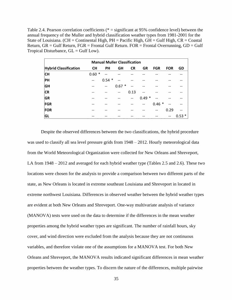
Table 2.4. Pearson correlation coefficients (* = significant at 95% confidence level)

between the annual frequency of the Muller and hybrid classification weather

types from 1981-2001 for the State of Louisiana. (CH = Continental High,

PH = Pacific High, GH = Gulf High, CR = Coastal Return, GR = Gulf Return,

FGR = Frontal Gulf Return. FOR = Frontal Overrunning, GD = Gulf Tropical

Disturbance, GL = Gulf Low). .........................................................................................35

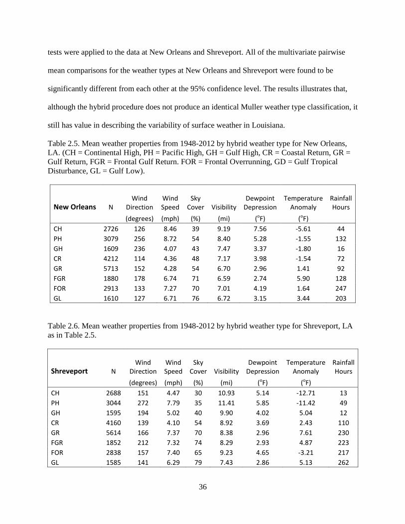
Table 2.5. Mean weather properties from 1948-2012 by hybrid weather type for New

Orleans, LA. (CH = Continental High, PH = Pacific High, GH = Gulf High,

CR = Coastal Return, GR = Gulf Return, FGR = Frontal Gulf Return,

FOR = Frontal Overrunning, GD = Gulf Tropical Disturbance, GL = Gulf Low) ............36

Table 2.6. Mean weather properties from 1948-2012 by hybrid weather type for

Shreveport, LA as in Table 2.5 ..........................................................................................36

Table 3.1. The amount of precipitation variance (R2) explained by synoptic frequency

for the nine Louisiana climate divisions for winter, spring, summer, and fall

determined using regression models. The data is expressed as percentages. ....................59

Table 3.2. The Durbin-Watson Statistic for the multiple linear regression models for

each season and climate division .......................................................................................61

vi

LIST OF FIGURES

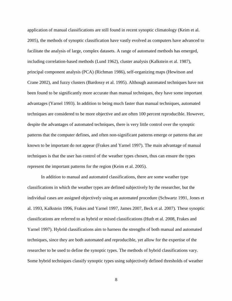
Figure 2.1. A 20oN –55

oN by 60

oW – 135

oW subset of the NCAR/NCEP Reanalysis I

dataset grid overlaid on the continental United States .......................................................11

Figure 2.2. Examples of sea level pressure patterns showing isobars, high and low

pressure centers, and fronts for each of the 8 original Muller Weather Types

(From Muller and Willis 1983) ..........................................................................................13

Figure 2.3. A flowchart of a correlation based classification of map patterns in

synoptic climatology. (Figure from Frakes and Yarnel 1997) ...........................................18

Figure 2.4. The subsets of the NCAR/NCEP reanalysis gridded dataset that were

used in the correlation procedure .......................................................................................20

Figure 2.5. Muller Sea Level Pressure Composites created using grids from the

testing dataset. (CH = Continental High, PH = Pacific High, GH = Gulf High,

CR = Coastal Return, GR = Gulf Return, FGR = Frontal Gulf Return.

FOR = Frontal Overrunning, GTD = Gulf Tropical Disturbance) ....................................23

Figure 2.6. Sea level pressure composites by weather type for the a) Muller and

b) hybrid classifications. The red bounding box shows the grid area used in the

classification algorithm. (CH = Continental High, PH = Pacific High, GH = Gulf

High, CR = Coastal Return, GR = Gulf Return, FGR = Frontal Gulf Return.

FOR = Frontal Overrunning, GTD = Gulf Tropical Disturbance, GL = Gulf Low). .......25

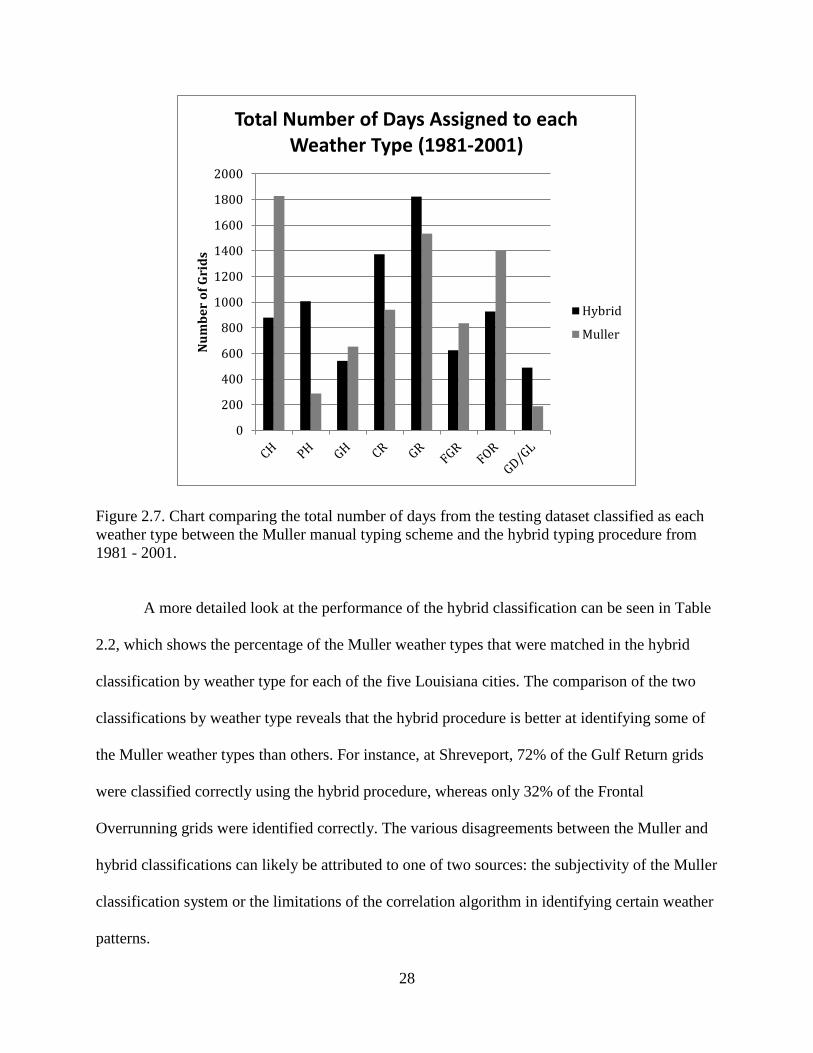
Figure 2.7. Chart comparing the total number of days from the testing dataset classified

as each weather type between the Muller manual typing scheme and the hybrid

typing procedure from 1981 – 2001...................................................................................28

Figure 2.8. Graphs comparing the seasonal frequency of the Muller and hybrid classifications

from 1981-2001. (CH = Continental High, PH = Pacific High, GH = Gulf High, CR =

Coastal Return, GR = Gulf Return, FGR = Frontal Gulf Return. FOR = Frontal

Overrunning, GD = Gulf Tropical Disturbance, GL = Gulf Low). ...................................32

Figure 2.9. Graphs comparing the annual frequency of the Muller and hybrid classifications

from 1981-2001. (CH = Continental High, PH = Pacific High, GH = Gulf High,

CR = Coastal Return, GR = Gulf Return, FGR = Frontal Gulf Return. FOR = Frontal

Overrunning, GD = Gulf Tropical Disturbance, GL = Gulf Low). ...................................34

Figure 3.1. NCDC Climate Divisions of Louisiana. (Image courtesy of the Louisiana

Office of State Climatology) ..............................................................................................50

vii

Figure 3.2. Winter normals and daily precipitation anomalies for Continental High(CH),

Pacific High(PH), Gulf High(GH), Coastal Return(CR), Gulf Return(GR),

Frontal Gulf Return(FGR), Frontal Overunning(FOR), and Gulf Low(GL)

weather types from 1948 – 2012 ........................................................................................55

Figure 3.3. Spring normals and Daily Precipitation anomalies as in Figure 3.2 ...........................56

Figure 3.4. Summer normals and Daily Precipitation anomalies as in Figure 3.2 ........................57

Figure 3.5. Fall normals and Daily Precipitation anomalies as in Figure 3.2 ................................58

Figure 3.6. Smoothed winter modeled and observed precipitation for each climate

division from 1956-2005....................................................................................................63

Figure 3.7. Smoothed spring modeled and observed precipitation for each climate

division from 1955-2005....................................................................................................64

Figure 3.8. Smoothed summer modeled and observed precipitation for each climate

division from 1955-2005....................................................................................................65

Figure 3.9. Smoothed fall modeled and observed precipitation for each climate

division from 1955-2005....................................................................................................66

Figure A.1. Histogram of Winter Regression Model Residuals for the A) Northwest

B) North Central C) Northeast D) West Central E) Central F) East Central

G) Southwest H) South Central I) Southeast Climate Divisions .......................................81

Figure A.2. Histogram of Spring Regression Model Residuals for the A) Northwest

B) North Central C) Northeast D) West Central E) Central

F) East Central G) Southwest H) South Central I) Southeast Climate Divisions ..............82

Figure A.3. Histogram of Summer Regression Model Residuals for the A) Northwest



Figure A.4. Histogram of Fall Regression Model Residuals for the A) Northwest



Figure A.5. Winter Regression Model Residuals vs. Winter Precipitation Estimates for

the A) Northwest B) North Central C) Northeast D) West Central E) Central


viii

Figure A.6. Spring Regression Model Residuals vs. Spring Precipitation Estimates for



Figure A.7. Summer Regression Model Residuals vs. Summer Precipitation Estimates for



Figure A.8. Fall Regression Model Residuals vs. Fall Precipitation Estimates for



ix

ABSTRACT

An automated synoptic weather classification system, based on the weather types devised

by Robert Muller for Louisiana, is presented in this thesis and an application of the classification

system to precipitation variability in Louisiana is demonstrated. The automated classification

presented here is a hybrid classification system that uses sea level pressure composites for each

Muller weather type as seeds in a correlation procedure to classify daily NCEP/NCAR

Reanalysis sea level pressure patterns. The resulting hybrid classification is automated, objective,

and has value in describing the surface weather variability in Louisiana. In the second part of this

research project, the newly developed hybrid classification system is used to establish

relationships between synoptic weather types and precipitation variability in Louisiana. Weather

types that produce precipitation in Louisiana are identified and, using linear regression models,

the frequency of rainy weather types is used to predict seasonal rainfall for each of the nine

Louisiana climate divisions. Averaged among all climate divisions, synoptic weather type

frequency accounts for 25% of the interannual precipitation variability in winter, 14% in spring,

19% in summer, and 25% in fall. While the models are better at predicting the decadal scale

variability and trends during fall and winter, these results indicate that synoptic frequency alone

is insufficient to describe precipitation variability in Louisiana. Future work will need to identify

additional predictors. However, the automated hybrid classification system presented in this

study can be used for many additional applications in historical and future climate research for

Louisiana.

1

CHAPTER 1. INTRODUCTION

1.1 Background

Louisiana is located in the Southeast United States, a region that is characterized by large

shifts in weather conditions from year to year, especially in terms of precipitation. One common

way to study weather variability for a location is using synoptic climatology. Synoptic

climatology is a sub-field of climatology that focuses on establishing relationships between

synoptic scale atmospheric circulation patterns and the surface environment (Yarnel 1993). The

primary methodology of synoptic climatology is synoptic classification, or the grouping of

similar circulation patterns into classes called synoptic types. In most contexts, a circulation

pattern is a field of some atmospheric variable, often sea level pressure or geopotential height

(Huth et al. 2008). There are a wide variety of different synoptic classification methodologies

and schemes, which are discussed in more detail in Chapter 2. The choice of synoptic

classification for use in a particular study is dependent on a variety of factors including study

region, weather phenomena, research question, etc. Oftentimes, a researcher will develop their

own unique classification scheme to match their research purposes.

Since there is a limited amount of synoptic climatological research in the south central

United States, it is still unclear how much synoptic type variability contributes to surface climate

variability and trends in Louisiana. Only one synoptic weather typing system exists exclusively

for Louisiana climate related studies; the Muller weather typing system for Louisiana (Muller

1977). While this system has been successful for many applications, it is a manual system that is

both subjective and time-consuming. The Muller system has limited applicability for studying

long term and/or future climate impacts. This thesis will present an automated classification

system for classifying synoptic weather typing system for Louisiana that attempts to capture the

2

essence of the Muller system. Automated classification systems open up many additional

applications by providing a fast, objective way to produce long-term synoptic type catalogs for a

region. Having the ability to produce large datasets broadens the scope of potential research to

include applications that require long term data, such as establishing relationships between

synoptic type frequency and surface phenomena. These applications are very important in

climate change research and can serve as the basis for a relatively new area of research

investigating synoptic types in future climates using general circulation models (GCMs), as well

as synoptic-based statistical downscaling of GCM projections. In particular, the discovery of

statistical relationships between variables that are less accurately portrayed by the GCMs, like

precipitation, are of great interest for statistical downscaling (Lee 2012).

For Louisiana, the various GCM’s disagree about the sign and magnitude of future

precipitation changes (Keim et al. 2011, Kunkel et al. 2013), likely due to process-based errors in

the models (Hope 2006, Finnis et al. 2009). As a result, until precipitation dynamics in the

models are improved substantially, statistical downscaling based on more accurately predicted

GCM variables is the only option to generate accurate precipitation predictions (Lee 2012). One

type of statistical downscaling is synoptic-based statistical downscaling, where models use

synoptic type frequency to predict surface variables. However, this is only a viable option if

there is a strong relationship between synoptic type and the surface variable in question. There

has yet to be a study investigating the statistical link between synoptic type frequency and

precipitation in Louisiana. However, precipitation has been broadly linked to synoptic-scale

controls (Muller 1977, Trewartha 1981, Keim 1996). By quantifying the relationship between

synoptic types and precipitation in Louisiana, this study will serve as the first step in evaluating

3

the feasibility of developing a statistical downscaling model for the region. Therefore, the

objectives of this thesis are:

1. Develop an automated synoptic classification system that will have wide reaching

climate and weather applications for Louisiana.

2. Use the newly developed classification system to study the influence of synoptic scale

weather variability on interannual to decadal scale precipitation variability in Louisiana.

1.2 Summary

The second chapter of this thesis presents a new method of synoptic classification for

Louisiana. The requirements for the classification system are 1) that it has wide applicability to

Louisiana weather and climate investigations and 2) that it is able to classify weather patterns

both quickly and objectively. The proposed method is an objectification of the Muller Weather

Typing system for Louisiana, a widely used manual classification system in the region for

applications ranging from air quality research (Muller and Jackson 1985) to the quantifying the

effect of El Niño-Southern Oscillation events on weather type frequencies (McCabe and Muller

2002). The goal of the procedure is not to recreate the Muller weather typing system, but to

develop a new classification system that is able produce a synoptic type catalog that describes

the synoptic variability of Louisiana in a way that is consistent with the manual Muller Weather

Types, yet has the advantages of being both objective and automated. The third chapter of this

thesis is an application of the newly developed classification system to study precipitation

variability in Louisiana. In Chapter 3, regression models are developed using synoptic type

frequency to predict seasonal rainfall for Louisiana’s climate divisions. By investigating the

statistical relationships between synoptic weather types and rainfall in Louisiana, this study is a

first step toward creating improved climate change projections for precipitation in the Louisiana.

4

Lastly, Chapter 4 includes a summary of findings and a discussion of future work related to this

project.

1.3 References

Finnis, J., J. Cassano, M. Holland, M. Serreze & P. Uotila (2009) Synoptically Forced

Hydroclimatology of Major Arctic Watersheds in General Circulation Models; Part 1:

The Mackenzie River Basin. International Journal of Climatology, 29, 1226-1243.

Hope, P. K. (2006) Projected Future Changes in Synoptic Systems Influencing Southwest

Western Australia. Climate Dynamics, 26, 765-780.

Huth, R., C. Beck, A. Philipp, M. Demuzere, Z. Ustrnul, M. Cahynova, J. Kysely & O. E. Tveito.

2008. Classifications of Atmospheric Circulation Patterns Recent Advances and

Applications. In Trends and Directions in Climate Research, eds. L. Gimeno, R.

GarciaHerrera & R. M. Trigo, 105-152. Oxford: Blackwell Publishing.

Keim, B. D. (1996) Spatial, Synoptic, and Seasonal Patterns of Heavy Rainfall in the

Southeastern United States. Physical Geography, 17, 313-328.

Keim, B. D., R. Fontenot, C. Tebaldi & D. Shankman (2011) Hydroclimatology of the Us Gulf

Coast under Global Climate Change Scenarios. Physical Geography, 32, 561-582.

Kunkel, K. E., L. E. Stevens, S. E. Stevens, L. Sun, E. Janssen, D. Wuebbles, C. E. K. II, C. M.

Fuhrman, B. D. Keim, M. C. Kruk, A. Billiot, H. Needham, M. Shafer & J. G. Dobson.

2013. Regional Climate Trends and Scenarios for the U.S. National Climate Assessment

Part 2. Climate of the Southeast U.S. In NOAA Technical Report NESDIS 142-2.

Lee, C. C. (2012) Utilizing Synoptic Climatological Methods to Assess the Impacts of Climate

Change on Future Tornado-Favorable Environments. Natural Hazards, 62, 325-343.

McCabe, G. J. & R. A. Muller (2002) Effects of Enso on Weather-Type Frequencies and

Properties at New Orleans, Louisiana, USA. Climate Research, 20, 95-105.

Muller, R. A. (1977) A Synoptic Climatology for Environmental Baseline Analysis: New

Orleans. Journal of Applied Meteorology 16, 20-33.

Muller, R. A. & A. L. Jackson (1985) Estimates of Climatic Air-Quality Potential at Shreveport,

Louisiana. Journal of Climate and Applied Meteorology, 24, 293-301.

5

Trewartha, G. 1981. The Earth's Problem Climates. The University of Wisconsin Press.

Yarnel, B. 1993. Synoptic Climatology in Environmental Analyis. London: Belhaven Press.

6

CHAPTER 2. AN AUTOMATED PROCEDURE FOR CLASSIFYING SYNOPTIC TYPES

FOR LOUISIANA, USA BASED ON THE MANUAL MULLER WEATHER TYPING

SCHEME

2.1 Abstract

This study presents an automated hybrid synoptic classification procedure for classifying

Louisiana weather types, based on the manual weather typing system devised by Robert Muller.

The goal of the procedure is to produce a synoptic classification system for Louisiana that

harnesses the strengths of both manual and automated classifications, while eliminating the

weaknesses. The Muller weather types archive from 1981 – 2001 is used in conjunction with the

NCEP/NCAR Reanalysis dataset to develop sea level pressure composites for each Muller

weather type. The composites are used as seeds in an automated correlation-based algorithm to

generate weather types from 1981-2001. Results of the automated procedure are compared to the

Muller weather type catalog. Despite systematic differences between the two classifications, the

automated procedure correctly matched the Muller weather type at one or more of the point

locations for 57% of the days. In addition, the automated catalog captured the seasonal

distribution and interannual variability of the Muller types remarkably well. The hybrid synoptic

weather classification system applied to weather properties at Shreveport and New Orleans

showed significant differences between weather types, demonstrating that although the

automated procedure does not replicate the Muller weather type classification exactly, it is

homogenous within itself and has value for describing the variability of surface weather in

Louisiana. In fact, it is arguably advantageous for some applications, due to its objectivity,

speed, and reproducibility.

7

2.2 Introduction

Synoptic classification is a commonly used approach within the field of climatology. It

focuses on establishing relationships between synoptic scale atmospheric circulation patterns and

the surface environment (Yarnel 1993). Synoptic scale features that make up the atmospheric

circulation pattern are generally between 1000 to 2500 kilometers in size (Huschke 1959), and

include ridges, troughs, cyclones, and anticyclones. The location and strength of synoptic

features can be indicative of the occurrence of different surface meteorological phenomena. In

fact, various sectors of cyclones and anticyclones can produce dramatically different weather

conditions (Keim et al. 2005). To capture this variability, synoptic patterns reduce the complex

atmosphere into a manageable number of discrete reoccurring patterns, or synoptic types (Yarnel

1993). Synoptic classification is a useful tool for climatological research, and has a wide range of

applications. Examples of applications include studying the relationship of synoptic types to

precipitation occurrence (Fragoso and Gomes 2008, Bettolli et al. 2010, Raziei et al. 2012),

linking synoptic type frequency to Pacific teleconnection frequency (Coleman and Rogers 2007),

investigating synoptic types in future climates using general circulation models (GCMs) (Hope

2006), and synoptic-based statistical downscaling of GCM projections (Wetterhall et al. 2009),

among many others.

There are many different techniques used to perform synoptic classification. However,

each classification follows the same general procedure of defining classification types and then

assigning each individual map pattern to a type (Huth et al. 2008). The earliest classifications

were done manually and are implicitly subjective (Hess and Brezowsky 1952, Lamb 1972,

Muller 1977). These classifications depended greatly on the experience of the researcher to

recognize important patterns (Huth et al. 2008, Yarnel 1993). While the development and

8

application of manual classifications are still found in recent synoptic climatology (Keim et al.

2005), the methods of synoptic classification have vastly evolved as computers have advanced to

facilitate the analysis of large, complex datasets. A range of automated methods has emerged,

including correlation-based methods (Lund 1962), cluster analysis (Kalkstein et al. 1987),

principal component analysis (PCA) (Richman 1986), self-organizing maps (Hewitson and

Crane 2002), and fuzzy clusters (Bardossy et al. 1995). Although automated techniques have not

been found to be significantly more accurate than manual techniques, they have some important

advantages (Yarnel 1993). In addition to being much faster than manual techniques, automated

techniques are considered to be more objective and are often 100 percent reproducible. However,

despite the advantages of automated techniques, there is very little control over the synoptic

patterns that the computer defines, and often non-significant patterns emerge or patterns that are

known to be important do not appear (Frakes and Yarnel 1997). The main advantage of manual

techniques is that the user has control of the weather types chosen, thus can ensure the types

represent the important patterns for the region (Keim et al. 2005).

In addition to manual and automated classifications, there are some weather type

classifications in which the weather types are defined subjectively by the researcher, but the

individual cases are assigned objectively using an automated procedure (Schwartz 1991, Jones et

al. 1993, Kalkstein 1996, Frakes and Yarnel 1997, James 2007, Beck et al. 2007). These synoptic

classifications are referred to as hybrid or mixed classifications (Huth et al. 2008, Frakes and

Yarnel 1997). Hybrid classifications aim to harness the strengths of both manual and automated

techniques, since they are both automated and reproducible, yet allow for the expertise of the

researcher to be used to define the synoptic types. The methods of hybrid classifications vary.

Some hybrid techniques classify synoptic types using subjectively defined thresholds of weather

9

variables for each type (Schwartz 1991, Kalkstein 1996). Other hybrid techniques are automated

versions of manual classifications, such as the Bergen school mid-latitude cyclone model (Frakes

and Yarnel 1997), the Hess and Brezowsky Grosswetterlagen for central Europe (James 2007),

and the Lamb Weather Types for the British Isles (Beck et al. 2007, Jones et al. 1993). These

types of hybrid classifications are created using pattern correlation between prototypes of each

weather type and the individual cases (Huth et al. 2008). These classifications are useful because

the manual classifications they are based on are well-known and are proven to describe

atmospheric variability well for their prospective regions. In a comparison study of the ability of

74 weather type classifications to identify associations of weather types with drought in

northwest Europe, the objectivized Grosswetterlagen (James 2007), a hybrid map pattern

classification, outperformed all other classification methods, even the manual Grosswetterlagen

(Fleig et al. 2010).

This paper centers on objectivizing a manual weather typing scheme for Louisiana that

was developed in the 1970s by Muller (1977). The Muller weather types are a very unique

synoptic type catalog and have a wide array of applications (Muller and Jackson 1985, McCabe

and Muller 1987, Faiers 1988, Faiers 1993, Faiers et al. 1994, Rohli and Henderson 1997,

McCabe and Muller 2002). The applications of the Muller weather range from studying the

effect of the El Nino Southern Oscillation on synoptic type frequency and properties of winter

precipitation in New Orleans (McCabe and Muller 2002), to evaluating air quality potential at

Shreveport, LA(Muller and Jackson 1985), to creating an index of evaporation by weather type

for Southern Louisiana (McCabe and Muller 1987). While the Muller weather type catalog is

useful for climate studies, its temporal coverage is limited, and types have not been cataloged in

over 10 years. This study aims to use a correlation-based hybrid synoptic classification

10

procedure, similar to that used by Frakes and Yarnel (1997), to blend the Muller Weather Typing

scheme for Louisiana with an automated correlation based classification technique. Furthermore,

this research will determine whether the hybrid procedure outlined below produces a synoptic

type system that describes the synoptic variability of Louisiana in a way that is consistent with

the manual Muller weather types. A successful automated hybrid procedure using the Muller

weather types as prototypes could be used to generate a long-term weather type catalog for

Louisiana, including intra-diurnal classifications of weather types. The resultant catalog will

provide a baseline for studying climate trends and their impacts in the region. In addition, the

hybrid method will be appropriate for studying climate model output and for further application

in synoptic climatology, especially since the Muller catalog is no longer maintained.

2.3 Data

2.3.1 NCEP/NCAR Reanalysis Dataset

This study utilizes sea level pressure data from the National Center for Atmospheric

Research (NCAR)/National Centers for Environmental Prediction (NCEP) Reanalysis I Dataset

(Kalnay et al. 1996). This dataset was assembled from a variety of climate data sources,

including land surface, satellite, aircraft, and rawinsonde data (Kalnay et al. 1996). There are

many different atmospheric variables included in the dataset, including both surface and upper-

air data. These data are available 4 times daily at six-hourly intervals (6Z, 12Z, 18Z, 00Z) from

1948 to present. The data are in the form of global grids, with 2.5 degree grid spacing. An

example of the data grid overlaid on the continental United States can be found in Figure 2.1. All

of the sea level pressure maps in this thesis show surfaces interpolated from gridded datasets.

11

Figure 2.1. A 20oN –55

oN by 60

oW – 135

oW subset of the NCAR/NCEP Reanalysis I dataset

grid overlaid on the continental United States.

2.3.2 Muller Weather Type Catalog

The Muller weather typing scheme for Louisiana was developed in the 1970s by Robert

Muller and maintained until mid-2002 by the Louisiana Office of State Climatology (LOSC). A

manual synoptic classification was produced for 0600 and 1500 CST (12Z and 21Z) for New

Orleans from January 1, 1961 – October 31, 2002 and for Shreveport, Monroe, Baton Rouge, and

Lake Charles from January 1, 1981 – October 31, 2002. The Muller Weather Typing scheme is a

subjective classification of surface maps, based primarily on pressure patterns and the location of

fronts; however, the researcher also takes into account certain local climate parameters, including

temperature, precipitation, clouds, relative humidity and winds, when assigning each surface

map to a weather type. Therefore, there are instances in which the entire state is experiencing the

same weather type and other times when 2 or more weather types are present within the state at

the same time. For this reason, the weather types were determined separately for each individual

12

city or point location. The eight Muller Weather types are briefly described below as they were

outlined in Muller and Willis (1983) with examples shown in Figure 2.2.

1. Continental High (CH): This weather type is characterized by surface high pressure over

the central US extending down into Louisiana, which causes north to northeasterly winds

over the region. The weather associated with this type is fair and cold.

2. Pacific High (PH): This weather type occurs in Louisiana after the passage of a Pacific

cold front. Normally, a surface low pressure system is situated to the northwest of the

region, causing west to northwest winds to usher in dry air over Louisiana. The typical

weather associated with this type is fair and mild.

3. Gulf High (GH): This weather type occurs when a high pressure system is located south

of Louisiana over the Gulf of Mexico. In these situations, the location of the high

pressure system causes southwest surface winds and brings fair and warm weather to

Louisiana.

4. Coastal Return (CR): This weather type occurs when a high pressure system is located to

the northeast of the region. This pattern causes easterly winds and brings fair and mild

weather to Louisiana.

5. Gulf Return (GR): This weather type occurs when a surface high pressure system moves

far enough east of the region to cause the surface winds over Louisiana to shift to

southeasterly, ushering in warm, moist air from the Gulf of Mexico. In addition, the

pressure gradient is often enhanced by a developing low pressure system over Texas. The

weather associated with this weather type in Louisiana is fair, warm, and humid.

13

Figure 2.2. Examples of sea level pressure patterns showing isobars, high and low pressure

centers, and fronts for each of the 8 original Muller Weather Types (From Muller and Willis

1983).

14

6. Frontal Gulf Return (FGR): This weather type is characterized by a frontal low pressure

system that is close enough to the region to affect its weather. Normally, an approaching

low pressure system causes south to southwest winds, and brings turbulent and stormy

weather to Louisiana.

7. Frontal Overrunning (FOR): This weather type occurs when a front becomes stationary

along the northern Gulf coast. Often during this kind of pattern, waves of low pressure

form and move eastward along the front. Normally, this weather type brings northeasterly

winds and rain to the region.

8. Gulf Tropical Disturbance (GTD): This weather type occurs when a tropical system,

ranging from a tropical wave to a Category 5 hurricane, impacts Louisiana. This weather

type brings strong, shifting winds and rainy weather to the region.

An archive of Muller weather types for Louisiana was created and maintained by Robert

Muller and his students until early 2002. Dr. Muller originally began the classification in the

1970’s. He later trained his students to use the system, and they extended the classification for

New Orleans back to 1961. Additionally, in the late 1990’s and early 2000’s, Dr.Muller’s

students assisted in weather typing for all cities. The entire archive was utilized in this study.

2.4 Automated Muller Weather Typing Procedure

2.4.1 Muller Weather Types Sea Level Pressure Composites

A weakness of automated synoptic typing techniques is the loss of valuable

climatological expertise in defining meaningful synoptic types for a region, inherent in manual

classifications. By using composite sea level pressure grids for each Muller weather type as

seeds in a correlation-based synoptic typing algorithm, we preserve the valuable researcher

knowledge that was used to define the Muller synoptic types in the manual typing procedure.

15

Daily sea level pressure data were collected from the NCAR/NCEP Reanalysis dataset for the

region from 20oN –50

oN by 65

oW – 125

oW from 1948 to 2012. This area covers the entire

continental United States, as well as the Gulf of Mexico. To create the composite sea level

pressure grids for each Muller type, a 21-year subset of the 12Z Muller synoptic type catalog

from 1981 to 2001, maintained in the Louisiana Office of the State Climatology and Southern

Regional Climate Center, was used to assign each corresponding NCEP/NCAR Reanalysis I

daily sea level pressure grid to the correct Muller weather type. This subset is referred to as the

training dataset. The time period from 1981 to 2001 was chosen because the Muller weather type

archive includes types for all five cities starting in 1981, with 2001 as the last full year of data

available. The training dataset was then refined to include only “non-transition” days, or days on

which the Muller synoptic type was the same at all 5 locations: Shreveport, Monroe, Lake

Charles, Baton Rouge, and New Orleans. The choice to include only “non-transition” days in the

calculation of the Muller weather type composites was made to ensure separation between the

types by preventing the influence sea level pressure grids that were in transition between two

weather type situations. Of the 7670 0600 CST sea level pressure grids from 1981 – 2001, 4202

of them were “non-transition”.

Using the grids from the training dataset, the average sea level pressure field for each

Muller weather type was calculated. Since there are seasonal differences in sea level pressure

pattern intensity, each sea level pressure grid was standardized before the seasonal means were

calculated. According to the study of Yarnel (1993), standardization is necessary to remove the

seasonal influences on absolute pressure patterns so that only the generalized map pattern

remains, making seasonal pressure patterns from different seasons comparable. Each daily sea

level pressure grid was standardized using the following formula known as the Z-transformation:

16

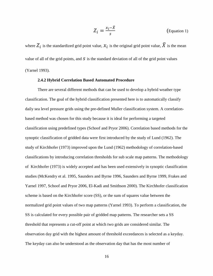
(Equation 1)

where is the standardized grid point value, is the original grid point value, is the mean

value of all of the grid points, and is the standard deviation of all of the grid point values

(Yarnel 1993).

2.4.2 Hybrid Correlation Based Automated Procedure

There are several different methods that can be used to develop a hybrid weather type

classification. The goal of the hybrid classification presented here is to automatically classify

daily sea level pressure grids using the pre-defined Muller classification system. A correlation-

based method was chosen for this study because it is ideal for performing a targeted

classification using predefined types (Schoof and Pryor 2006). Correlation based methods for the

synoptic classification of gridded data were first introduced by the study of Lund (1962). The

study of Kirchhofer (1973) improved upon the Lund (1962) methodology of correlation-based

classifications by introducing correlation thresholds for sub scale map patterns. The methodology

of Kirchhofer (1973) is widely accepted and has been used extensively in synoptic classification

studies (McKendry et al. 1995, Saunders and Byrne 1996, Saunders and Byrne 1999, Frakes and

Yarnel 1997, Schoof and Pryor 2006, El-Kadi and Smithson 2000). The Kirchhofer classification

scheme is based on the Kirchhofer score (SS), or the sum of squares value between the

normalized grid point values of two map patterns (Yarnel 1993). To perform a classification, the

SS is calculated for every possible pair of gridded map patterns. The researcher sets a SS

threshold that represents a cut-off point at which two grids are considered similar. The

observation day grid with the highest amount of threshold exceedances is selected as a keyday.

The keyday can also be understood as the observation day that has the most number of

17

observational days with similar sea level pressure grids. Keydays represents typical synoptic

patterns (Yarnel 1993). Next, the keydays and all similar days are removed from the dataset, and

the process is repeated until there are no days left. Each observation is then assigned to the

keyday for which it has the highest SS value above the chosen threshold. If an observation has no

SS value above the threshold, it is considered unclassified (Yarnel 1993). The choice of

correlation threshold impacts how many keydays are chosen, how many unclassified days there

are in the classification, and the within and between group variance of the weather types (Yarnel

1993). An overview of a correlation based classification procedure in synoptic climatology is

presented in Figure 2.3.

The classification performed in this study is a targeted Kirchhofer classification (Frakes

and Yarnel 1997, Schoof and Pryor 2006). Instead of allowing the algorithm to define the

keydays as in a traditional Kirchhofer classification, keydays were predefined as the Muller sea

level pressure composites. Therefore, the choice of correlation threshold has no impact on the

number of keydays chosen. Theoretically, the choice of correlation threshold is still important in

a targeted Kirchhofer classification. Higher correlation thresholds should minimize within group

variance, but result in a high number of unclassified days, whereas lower correlation thresholds

result in higher within group variance with a lower number of unclassified days. However, the

study of Frakes and Yarnel (1997) found no significant advantages in minimizing within group

variance by choosing higher correlation thresholds over lower correlation thresholds with much

higher percentages of days classified. In fact, they found that the within-group variance of the

hybrid weather types with a correlation threshold of r = 0.00 was actually less than the within-

group variance of the manual classification weather types. For this reason, I chose to eliminate

18

Figure 2.3. A flowchart of a correlation based classification of map patterns in synoptic

climatology. (Figure from Frakes and Yarnel 1997).

19

the correlation thresholds from the classification procedure and simply assign each observation

to the keyday that had the lowest SS value. To determine the most appropriate weather type, the

SS was calculated between an individual sea level pressure grid and each Muller sea level

pressure composite grid, using the formula:

∑ ( )

(Equation 2)

where SS is the Sum of Squares or Kirchhofer score, N is the number of grid points, Gxi is the

normalized value of grid point i on sea level pressure grid x, and Myi is the normalized value of

grid point i on the Muller sea level pressure composite grid y (Yarnel 1993). Using this

procedure, all sea level pressure grids are classified. A variety of different sized subsets of the

gridded NCAR/NCEP Reanalysis data were experimented with for use in the sum of squares

procedure (Figure 2.4). Using each of the grid sizes, daily weather types were produced using the

procedure from 1981 to 2001 and compared with the Muller weather types. The table 2.1 reports

the percentages of days that had an exact weather type match between the Muller and hybrid

datasets for one or more of the point locations. It was found that when using gridded data that

covered the large areas, many of the features that are significant to Louisiana weather got

“washed out” by the variability of other synoptic features across the country, and fewer daily

matches occurred. On the other hand, the small grid that centered on Louisiana (H in Figure 2.4)

did not offer enough information about the synoptic conditions to produce a good classification.

20

Figure 2.4. The subsets of the NCAR/NCEP reanalysis gridded dataset that were used in the

correlation procedure.

Table 2.1. The coordinates and percentage of days that had an exact weather type match between

the Muller and hybrid weather classification catalogs for the grids shown in Figure 2.4.

Grid Upper Right Coordinates

Lower Left Coordinates

Daily Matches

A 50 N, -65 W 20 N, -125 W 55%

B 47.5 N, -87.5 W 22.5 N, -177.5 W 42%

C 47.5 N, -65 W 22.5 N, -95 W 43%

D 45 N, -70 W 25 N, -110 W 46%

E 37.5 N, -87.5 W 27.5 N , -110 W 50%

F 37.5 N, -75 W 20 N, -105 W 55%

G 35 N, -80 W 25 N, -100 W 57%

H 35 N, -87.5 W 27.5 N, -95 W 53%

21

Through trial and error, it was found that calculating the sum of squares between subsets

of the grids from 25oN –35

oN by 80

oW – 100

oW (G in Figure 2.4) produced a classification that

was the most similar to the manual Muller weather types on a daily time scale. This subset

covers a 1000 x 2000 kilometer area centered on New Orleans, LA. The hybrid procedure was

first used to classify only the sea level pressure grids in the training dataset, which includes all

12Z sea level pressure grids from 1981 – 2001. After the procedure was evaluated according the

methods described below, all 12Z sea level pressure grids from 1948 – 2012 were classified

using the hybrid procedure.

2.4.3 Evaluation of Hybrid Classification

The hybrid classification was first evaluated by comparing the automated and manual

classifications for each sea level pressure grid in the training dataset on a daily basis to determine

what percentage of the grids were classified as the same type using both methods. However, it is

important to note that the automated hybrid procedure defines weather types for the entire state,

whereas the Muller system defines weather types individually for each point location. This

difference makes it somewhat challenging to compare the two classifications. Since only one

classification was performed for the entire state in the hybrid procedure, results were compared

to the manual Muller classification at each of the 5 cities to determine if the hybrid procedure

performed better at some locations than at others. Monthly and annual frequencies of each

weather type were compared and correlation coefficients were calculated between datasets to

determine if the hybrid classification captured the same seasonal and annual distribution of

weather types as the Muller classification. Finally, using the hybrid classification catalog from

1948 – 2012, mean weather properties at each city (wind speed and direction, visibility, cloud

cover, temperature anomaly, dew point depression, and precipitation days) were calculated from

22

World Meteorological Organization (WMO) Surface Hourly Data for each hybrid weather type

to evaluate whether the hybrid classification captures differences in observed weather between

weather types. To further explore differences between the weather types, pairwise multivariate

tests for equality were conducted on the mean weather properties for each type.

2.5 Results and Discussion

2.5.1 Muller Weather Types Sea Level Pressure Composites

Sea level pressure composites for the eight Muller Weather Types are shown in Figure

2.5. For the most part, the composites capture the main synoptic level features that are

characteristic of each type and the wind flow over Louisiana is correct for most types. For

example, the sea level pressure composite for the Pacific High type has high pressure system in

the west and low pressure in the midwest, with northwesterly flow over Louisiana. This pattern

is similar to that described by Muller and Willis (1983) for a typical Pacific High pattern. This

holds true in most cases; however, one composite that does not have a very distinct pattern is the

Frontal Overrunning composite. This is likely because the location of the surface cold front is

important to delineating this weather type in the Muller classification, though these fronts are not

included in the pressure patterns of the NCEP Reanalysis dataset. As such, it will be difficult for

the automated procedure to distinguish it from some of the other weather types using pressure

patterns alone. The Gulf Tropical Disturbance sea level pressure composite detects low pressure

in the eastern Gulf, but the low pressure system is elongated and offset to the west of Louisiana.

This is likely due to the fact that there is a large amount of variability in tropical patterns,

23

Figure 2.5. Muller Sea Level Pressure Composites created using grids from the testing dataset.

(CH = Continental High, PH = Pacific High, GH = Gulf High, CR = Coastal Return, GR = Gulf

Return, FGR = Frontal Gulf Return. FOR = Frontal Overrunning, GTD = Gulf Tropical

Disturbance).

24

which range from weak tropical disturbances to major hurricanes, and can affect Louisiana from

any position in the Gulf of Mexico under a variety of atmospheric conditions. While this

composite should be able to identify most of the tropical systems in the automated classification,

it will also classify extra-tropical Gulf lows, which commonly form off the coast of Texas in

winter and spring (Hsu 1992), as Gulf Tropical Disturbances. Both of these weather patterns

cause disturbed weather in Louisiana, so instead of eliminating the pattern from the automated

classification, we chose to rename the class Gulf Low (GL) and accept that this will cause some

disagreement between the two classification systems.

2.5.2 Evaluation of Hybrid Classification

The 1981 to 2001 sea level pressure composites for both the Muller and hybrid

classifications are displayed in Figure 2.6. The red box indicates the grid that was used in the

automated procedure. If the hybrid classification was a perfect replica of the Muller

classification, the composites for each classification would be identical. While there are some

minor differences, such as the strength of the high and low pressure systems, the main synoptic

features are the same for both classifications. Most importantly, the orientation of the sea level

pressure gradient over Louisiana is very similar between the two classifications for each weather

type. This is important because the Muller classification relies heavily on wind direction, and the

pressure gradient orientation largely determines wind direction. The similarity between the

Muller and hybrid sea level pressure composites suggests that the hybrid system, while not

replicating the Muller system, may serve as an acceptable surrogate.

25

Figure 2.6. Sea level pressure composites by weather type for the a) Muller and b) hybrid

classifications. The red bounding box shows the grid area used in the classification algorithm.

(CH = Continental High, PH = Pacific High, GH = Gulf High, CR = Coastal Return, GR = Gulf

Return, FGR = Frontal Gulf Return. FOR = Frontal Overrunning, GTD = Gulf Tropical

Disturbance, GL = Gulf Low).

a) Manual Muller b) Hybrid

26

(Figure 2.6 continued)

a) Manual Muller b) Hybrid

27

A comparison of the Muller and hybrid classifications on a daily basis revealed that the

hybrid classification correctly matched the Muller weather type at one or more of the points. The

hybrid classification correctly identified the Muller weather type in 41% of the cases (Table 2.2).

The highest percentage classified correctly was 45 % at Lake Charles. At first consideration,

these figures seem low. It is important to remember that the purpose of a hybrid classification is

not to exactly replicate the original manual classification; instead, the goal is to provide an

acceptable alternate that can be used for applications that benefit from using automated

methodologies (Huth et al. 2008). In the hybrid classification literature, these results of this study

are comparable to the results of other similar studies. For example, the objectivized

Grosswetterlagen classification had a 39.1 % daily correspondence with the manual

Grosswetterlagen classification (James 2007). However, the classification is considered highly

successful. In fact, it outperformed over 70 other classifications in an inter-comparison study of

their power to analyze drought in north-western Europe. Other daily correspondence values

between manual classifications and their objectivized versions are 42 % in Frakes and Yarnel

(1997) and 34.7 % in Kruger (2002). Compared to these previous studies, the objectivized

Muller classification had slightly better success on the daily timescale at each point location.

Figure 2.7 shows the total number of days from the testing dataset assigned to each

weather type for each classification, with the number of Muller days presented as the average of

the number of days classified as each weather type at the five Louisiana cities. This figure shows

that the hybrid classification under classifies the Continental High and Frontal Overrunning

types, and over classifies the Pacific High and Gulf Disturbance types. Yet, the total number of

days classified as Gulf High, Coastal Return, Gulf Return, and Frontal Gulf Return types is

similar for both the Muller and hybrid Classifications.

28

Figure 2.7. Chart comparing the total number of days from the testing dataset classified as each

weather type between the Muller manual typing scheme and the hybrid typing procedure from

1981 - 2001.

A more detailed look at the performance of the hybrid classification can be seen in Table

2.2, which shows the percentage of the Muller weather types that were matched in the hybrid

classification by weather type for each of the five Louisiana cities. The comparison of the two

classifications by weather type reveals that the hybrid procedure is better at identifying some of

the Muller weather types than others. For instance, at Shreveport, 72% of the Gulf Return grids

were classified correctly using the hybrid procedure, whereas only 32% of the Frontal

Overrunning grids were identified correctly. The various disagreements between the Muller and

hybrid classifications can likely be attributed to one of two sources: the subjectivity of the Muller

classification system or the limitations of the correlation algorithm in identifying certain weather

patterns.

0

200

400

600

800

1000

1200

1400

1600

1800

2000

Nu

mb

er

of

Gri

ds

Total Number of Days Assigned to each Weather Type (1981-2001)

Hybrid

Muller

29

Table 2.2. A) The percentages of Muller classification grids by type from the testing dataset that

were classified as each of the weather types in the hybrid classification from 1981 – 2001 for

Shreveport, Monroe, Lake Charles, LA. B) Same, but for Baton Rouge, and New Orleans, LA.

A) Hybrid Classification CH PH GH CR GR FGR FOR GD

Shreveport

CH 34% 7% 6% 4% 1% 1% 7% 1%

PH 24% 55% 15% 1% 0% 4% 14% 1%

GH 4% 6% 43% 3% 6% 7% 2% 2%

CR 18% 3% 9% 51% 15% 9% 14% 13%

GR 2% 4% 21% 23% 72% 31% 8% 23%

FGR 1% 14% 3% 2% 4% 32% 10% 6%

FOR 15% 7% 2% 8% 0% 5% 32% 7%

GL 2% 3% 1% 8% 2% 10% 13% 46%

Total Agreement = 44%

Monroe

CH 33% 7% 5% 3% 0% 1% 7% 0%

PH 20% 58% 14% 1% 1% 5% 18% 1%

GH 4% 7% 43% 2% 5% 8% 2% 3%

CR 22% 4% 8% 47% 11% 8% 12% 8%

GR 4% 6% 25% 30% 72% 23% 8% 20%

FGR 1% 11% 3% 1% 8% 36% 8% 8%

FOR 13% 6% 2% 8% 0% 7% 33% 6%

GL 2% 1% 1% 8% 3% 12% 12% 53%


Lake Charles

CH 36% 6% 5% 5% 1% 2% 11% 1%

PH 23% 63% 16% 1% 1% 7% 17% 1%

GH 4% 5% 41% 3% 5% 3% 1% 3%

CR 20% 3% 9% 48% 20% 8% 16% 22%

GR 2% 4% 21% 26% 63% 17% 7% 20%

FGR 1% 10% 4% 2% 6% 36% 4% 6%

FOR 12% 5% 3% 9% 1% 13% 34% 9%

GL 2% 2% 1% 6% 3% 15% 9% 38%


30

(Table 2.2 continued)

B) Hybrid Classification CH PH GH CR GR FGR FOR GD

Baton Rouge

CH 34% 8% 5% 4% 0% 2% 12% 1%

PH 19% 65% 15% 1% 1% 12% 21% 2%

GH 4% 6% 40% 2% 5% 4% 2% 3%

CR 25% 3% 8% 44% 10% 5% 14% 17%

GR 5% 5% 25% 33% 61% 10% 7% 22%

FGR 1% 9% 3% 2% 16% 32% 3% 8%

FOR 11% 4% 2% 8% 2% 18% 33% 8%

GL 1% 1% 1% 5% 5% 17% 8% 39%


New Orleans

CH 35% 8% 4% 4% 0% 2% 14% 1%

PH 18% 65% 16% 1% 1% 15% 21% 1%

GH 5% 6% 40% 3% 5% 3% 2% 3%

CR 25% 3% 8% 43% 9% 5% 15% 18%

GR 6% 6% 25% 34% 60% 9% 7% 22%

FGR 0% 7% 3% 2% 17% 28% 2% 9%

FOR 10% 3% 2% 8% 2% 22% 32% 9%

GL 1% 1% 1% 5% 5% 16% 7% 37%


The seasonal frequency of the weather types was compared between the two

classifications (Figure 2.8). The Muller seasonal frequency values were computed as the average

of the seasonal frequency of each weather type at the five Louisiana cities. Similar to the daily

comparison, the seasonality of some of the weather types was captured better by the hybrid

procedure than others. However, considering the daily alliance of the Muller and hybrid

classifications was less than 60%, the seasonal distribution of the Muller weather types was

reproduced remarkably well in the hybrid classification. The Pearson’s correlation coefficient

31

was calculated between the Muller and hybrid seasonal frequencies for each weather type (Table

2.3). The seasonal frequencies of all weather types, except for Frontal Overrunning and Gulf

Tropical Disturbance/Gulf Low, for the Muller and hybrid classifications are significantly

correlated at the 95 % confidence level. This result could indicate that a large number of the

misclassified grids are assigned to a weather type with a similar sea level pressure pattern that is

just as likely to occur during a particular season. For example, while 40% of the Coastal Return

grids were classified correctly by the hybrid procedure at New Orleans, 25% of them were

assigned to the Gulf Return type (see Table 2.2). This is not that surprising, since the Coastal

Return Type often transitions into the Gulf Return Type when the high pressure system shifts

farther east of Louisiana. It is likely that some of the Coastal Return types in the Muller

Classification that were “mistyped” in the hybrid classification were in transition between

Coastal Return and Gulf Return. Since the Coastal Return and Gulf Return Types cause very

similar types of weather for Louisiana, this error is not really detrimental to the hybrid

classification. The major differences in seasonality between the two classifications are associated

with the Gulf Tropical Disturbance/Gulf Low and Frontal Overunning weather types. In the

Muller classification, the seasonal frequency of the Gulf Tropical Disturbance type is centered

on the hurricane season. However, in the hybrid classification, there are also baroclinic low

pressure systems included in this type, which occur from late fall to spring (Hsu 1992). This

helps to explain the double peak in the seasonality of the Gulf Low weather type in the hybrid

classification, one in spring and one in summer.

32

Figure 2.8. Graphs comparing the seasonal frequency of the Muller and hybrid classifications

from 1981-2001. (CH = Continental High, PH = Pacific High, GH = Gulf High, CR = Coastal

Return, GR = Gulf Return, FGR = Frontal Gulf Return. FOR = Frontal Overrunning, GD = Gulf

Tropical Disturbance, GL = Gulf Low).

CR

33

Table 2.3. Pearson correlation coefficients (* = significant at 95% confidence level) between the

seasonal frequency of the Muller and hybrid classification weather types from 1981 – 2001 for

the State of Louisiana. (CH = Continental High, PH = Pacific High, GH = Gulf High, CR =

Coastal Return, GR = Gulf Return, FGR = Frontal Gulf Return. FOR = Frontal Overrunning, GD

= Gulf Tropical Disturbance, GL = Gulf Low).

Manual Muller Classification

Hybrid Classification CH PH GH CR GR FGR FOR GD

CH 0.90 * -- -- -- -- -- -- --

PH -- 0.96 * -- -- -- -- -- --

GH -- -- 0.97 * -- -- -- -- --

CR -- -- -- 0.74 * -- -- -- --

GR -- -- -- -- 0.93 * -- -- --

FGR -- -- -- -- -- 0.93 * -- --

FOR -- -- -- -- -- -- 0.43 --

GL -- -- -- -- -- -- -- 0.44

The interannual variability of the weather types in the two classifications was evaluated

(Figure 2.9). The Muller annual frequency values were computed as the average of the

interannual frequency of each weather type at the five Louisiana cities. Similar to the previous

results reported, the interannual variability was captured by the hybrid procedure more

accurately for some weather types than for others; however, the annual comparisons showed less

covariability than the seasonal comparisons. The Pearson’s correlation coefficient was calculated

between the Muller and hybrid seasonal frequencies for each weather type (Table 2.4). Although

the correlations are not as strong for interannual variability as they are for seasonality, six of the

eight weather types have significant correlations at the 95 % confidence level. While the annual

hybrid time series captures most of the annual rainfall peaks in the Muller classification, it does

not always capture the same trends. For example, in the Muller classification, there is an

increasing precipitation trend in the Gulf Return type. This same trend is not evident in the

hybrid classification.

34

Figure 2.9. Graphs comparing the annual frequency of the Muller and hybrid classifications from

1981-2001. (CH = Continental High, PH = Pacific High, GH = Gulf High, CR = Coastal Return,

GR = Gulf Return, FGR = Frontal Gulf Return. FOR = Frontal Overrunning, GD = Gulf Tropical


35

Table 2.4. Pearson correlation coefficients (* = significant at 95% confidence level) between the

annual frequency of the Muller and hybrid classification weather types from 1981-2001 for the

State of Louisiana. (CH = Continental High, PH = Pacific High, GH = Gulf High, CR = Coastal

Return, GR = Gulf Return, FGR = Frontal Gulf Return. FOR = Frontal Overrunning, GD = Gulf

Tropical Disturbance, GL = Gulf Low).

Manual Muller Classification

Hybrid Classification CH PH GH CR GR FGR FOR GD

CH 0.60 * -- -- -- -- -- -- --

PH -- 0.54 * -- -- -- -- -- --

GH -- -- 0.67 * -- -- -- -- --

CR -- -- -- 0.13

-- -- -- --

GR -- -- -- -- 0.49 * -- -- --

FGR -- -- -- -- -- 0.46 * -- --

FOR -- -- -- -- -- -- 0.29 --

GL -- -- -- -- -- -- -- 0.53 *

Despite the observed differences between the two classifications, the hybrid procedure

was used to classify all sea level pressure grids from 1948 – 2012. Hourly meteorological data

from the World Meteorological Organization were collected for New Orleans and Shreveport,

LA from 1948 – 2012 and averaged for each hybrid weather type (Tables 2.5 and 2.6). These two

locations were chosen for the analysis to provide a comparison between two different parts of the

state, as New Orleans is located in extreme southeast Louisiana and Shreveport in located in

extreme northwest Louisiana. Differences in observed weather between the hybrid weather types

are evident at both New Orleans and Shreveport. One-way multivariate analysis of variance

(MANOVA) tests were used on the data to determine if the differences in the mean weather

properties among the hybrid weather types are significant. The number of rainfall hours, sky

cover, and wind direction were excluded from the analysis because they are not continuous

variables, and therefore violate one of the assumptions for a MANOVA test. For both New

Orleans and Shreveport, the MANOVA results indicated significant differences in mean weather

properties between the weather types. To discern the nature of the differences, multiple pairwise

36

tests were applied to the data at New Orleans and Shreveport. All of the multivariate pairwise

mean comparisons for the weather types at New Orleans and Shreveport were found to be

significantly different from each other at the 95% confidence level. The results illustrates that,

although the hybrid procedure does not produce an identical Muller weather type classification, it

still has value in describing the variability of surface weather in Louisiana.

Table 2.5. Mean weather properties from 1948-2012 by hybrid weather type for New Orleans,

LA. (CH = Continental High, PH = Pacific High, GH = Gulf High, CR = Coastal Return, GR =

Gulf Return, FGR = Frontal Gulf Return. FOR = Frontal Overrunning, GD = Gulf Tropical


New Orleans N Wind

Direction Wind Speed

Sky Cover Visibility

Dewpoint Depression

Temperature

Anomaly Rainfall Hours

(degrees) (mph) (%) (mi) (oF) (oF)

CH 2726 126 8.46 39 9.19 7.56 -5.61 44

PH 3079 256 8.72 54 8.40 5.28 -1.55 132

GH 1609 236 4.07 43 7.47 3.37 -1.80 16

CR 4212 114 4.36 48 7.17 3.98 -1.54 72

GR 5713 152 4.28 54 6.70 2.96 1.41 92

FGR 1880 178 6.74 71 6.59 2.74 5.90 128

FOR 2913 133 7.27 70 7.01 4.19 1.64 247

GL 1610 127 6.71 76 6.72 3.15 3.44 203

Table 2.6. Mean weather properties from 1948-2012 by hybrid weather type for Shreveport, LA

as in Table 2.5.

Shreveport N Wind

Direction Wind Speed

Sky Cover Visibility

Dewpoint Depression

Temperature

Anomaly Rainfall Hours

(degrees) (mph) (%) (mi) (oF) (oF)

CH 2688 151 4.47 30 10.93 5.14 -12.71 13

PH 3044 272 7.79 35 11.41 5.85 -11.42 49

GH 1595 194 5.02 40 9.90 4.02 5.04 12

CR 4160 139 4.10 54 8.92 3.69 2.43 110

GR 5614 166 7.37 70 8.38 2.96 7.61 230

FGR 1852 212 7.32 74 8.29 2.93 4.87 223

FOR 2838 157 7.40 65 9.23 4.65 -3.21 217

GL 1585 141 6.29 79 7.43 2.86 5.13 262

37

2.5.3 Limitations

One of the main limitations involved in automating a manual classification system is the

subjectivity of the original system, which causes a certain amount of variability within the

weather types. Although the Muller system had guidelines for assigning weather patterns to

particular weather types, the decision was ultimately up to the researcher. Sometimes, the choice

of one weather type over another in a particular situation was not distinct. It is also likely that the

researcher introduced slight changes to his technique over the years. To complicate matters,

various researchers were responsible for weather typing during certain time periods. One

example of subjectivity in the Muller classification system was the distinction between Pacific

and Continental High types. Patterns dominated by high pressure systems with Pacific origin

were classified as Pacific High weather types. Often, once these high pressure systems moved

eastward over the central US, the patterns that were originally Pacific High were then classified

as Continental High. Dr. Muller considered this change from Pacific High to Continental High to

occur when the wind at New Orleans shifted to the north (Rohli and Henderson 1997). Yet, this

distinction was very subjective. This particular example explains why a high percentage of the

Muller Continental High patterns are classified as Pacific High patterns in the Hybrid procedure

(see Table 2.2). One way to quantify the subjectivity of the original Muller system is to calculate

the within type variability for each weather type. Future work could investigate if the within type

variability varies between different time periods. For instance, is the within type variability

higher during periods when researchers other than Dr. Muller performed the classifications? Or,

does the within type variability decrease with time as Dr. Muller refines his technique? This type

of analysis could help refine the training dataset to only include a time period with low within

type variability, perhaps minimizing some of the error introduced into the hybrid procedure.

38

Another limitation in this study was the restriction of the correlation algorithm used to

perform the hybrid classification. Whereas the Muller system takes into account the local

observed weather properties and the placement of fronts, the hybrid system relies simply on the

sea level pressure pattern to assign types. This difference limits the ability of the correlation

algorithm to detect certain weather types. For example, there is a large disparity between the

Muller and hybrid systems for the Frontal Overrunning pattern, since the Muller system relied on

frontal placement to assign this type and there is no distinct pressure pattern for the correlation

algorithm to detect. Future research could incorporate different levels of the atmosphere into the

hybrid classification to help identify weather types. Specifically, for the Frontal Overrunning

type, there are some distinguishing features at 500 millibar geopotential height layer, such as

shortwave troughs that, in addition to the sea level pressure pattern, could help a correlation

algorithm identify the type correctly.

2.6 Summary and Conclusions

This study achieved the goal of producing a synoptic classification system for Louisiana

that harnesses the strengths of both manual and automated classifications. The objective Muller

weather typing system was used to classify daily 12Z NCEP/NCAR sea level pressure grids, and

sea level pressure composites were generated for each Muller weather type. These composites

were used as seeds in an automated correlation-based procedure to produce hybrid weather types

for Louisiana. Compared on a daily basis, the Muller weather types and the hybrid weather types

matched at one or more point locations on 57 % of the days in question. The hybrid classification

developed in this study performed slightly better than other similar hybrid classification efforts

on a daily time scale (Frakes and Yarnel 1997, James 2007). The hybrid classification was also

successful at reproducing the seasonal and annual variability of most of the Muller weather

39

types. The hybrid classification was applied to weather properties at New Orleans and

Shreveport, and significant differences were found between the mean weather properties of

different hybrid weather types, illustrating the classification has some ability to describe surface

weather variability in Louisiana.

While I consider the hybrid classification successful, it is important to note that it should

not be considered synonymous with the manual Muller classification. The inherent subjectivity

of the manual Muller classification system, as well as limitations of the correlation-based

procedure, prevented the hybrid procedure from directly replicating the Muller classification

system exactly. The most fundamental difference between the two classifications is that the

Muller classification is performed separately for individual point locations, so at any instance

different locations in the state can have different weather types than each other, while the hybrid

classification assigns a single weather type to the entire state. While the hybrid classification

catalog is homogeneous within itself, it is not recommended that it should be used to extend the

Muller weather type catalog. The capabilities of each classification are unique, and both are

valuable tools for studying the synoptic climatology of Louisiana. Unlike the manual Muller

weather typing scheme, the hybrid procedure can be used to classify thousands of sea level

pressure patterns in a matter of minutes, making it feasible to use this classification procedure to

study the long term, and even the future, climate. While other automated synoptic classification

methods have similar advantages, they lack any control over the definition of synoptic types.

Yet, the procedure outlined in this study captures the intent Dr. Robert Muller had about

classifying the weather patterns of Louisiana; therefore in this researcher’s opinion, provides a

better description of weather variability for the region than other automated techniques could

offer.

40

The hybrid classification system and the daily synoptic type catalog generated in this

study could be used for a wide range of climate related applications in Louisiana. These include,

but are not limited to, analyzing the frequency and variability of weather types, studying the

variability of surface weather phenomena, and investigating the effect of synoptic type

variability on ecological and biological processes. The hybrid classification is also well suited to

adaptation for use with GCM output. This opens up a whole suite of additional applications for

studying future climate in Louisiana. Establishing relationships between synoptic type frequency

and trends in surface phenomena is very important in climate change research and can serve as

the basis for a relatively new area of research investigating synoptic types in future climates

using GCMs. These relationships can be used to develop synoptic-based statistical downscaling

of GCM projections, which can provide more accurate projections for certain weather variables

than general GCM output (Lee 2012).

2.7 References

Bardossy, A., L. Duckstein & I. Bogardi (1995) Fuzzy Rule-Based Classification of Atmospheric

Circulation Patterns. International Journal of Climatology, 15, 1087-1097.

Beck, C., J. Jacobeit & P. D. Jones (2007) Frequency and within-Type Variations of Large-Scale

Circulation Types and Their Effects on Low-Frequency Climate Variability in Central

Europe since 1780. International Journal of Climatology, 27, 473-491.

Bettolli, M. L., O. C. Penalba & W. M. Vargas (2010) Synoptic Weather Types in the South of

South America and Their Relationship to Daily Rainfall in the Core Crop-Producing

Region in Argentina. Australian Meteorological and Oceanographic Journal, 60, 37-47.

Coleman, J. S. M. & J. C. Rogers (2007) A Synoptic Climatology of the Central United States

and Associations with Pacific Teleconnection Pattern Frequency. Journal of Climate, 20,

3485-3497.

El-Kadi, A. K. A. & P. A. Smithson (2000) Probability Assessment of Pressure Patterns over the

British Isles. International Journal of Climatology, 20, 1351-1369.

41

Faiers, G. E. (1988) A Synoptic Weather Type Analysis of January Hourly Precipitation at Lake

Charles, Louisiana. Physical Geography, 9, 223-231.

--- (1993) Diurnal Distribution of Hourly Rainfall Events During January by Synoptic Weather

Types at Lake-Charles, Louisiana. Texas Journal of Science, 45, 265-271.

Faiers, G. E., B. D. Keim & K. K. Hirschboeck (1994) A Synoptic Evaluation of Frequencies

and Intensities of Extreme 3-Hour and 24-Hour Rainfall in Louisiana. Professional

Geographer, 46, 156-163.

Fleig, A. K., L. M. Tallaksen, H. Hisdal, K. Stahl & D. M. Hannah (2010) Inter-Comparison of

Weather and Circulation Type Classifications for Hydrological Drought Development.

Physics and Chemistry of the Earth, 35, 507-515.

Fragoso, M. & P. T. Gomes (2008) Classification of Daily Abundant Rainfall Patterns and

Associated Large-Scale Atmospheric Circulation Types in Southern Portugal.

International Journal of Climatology, 28, 537-544.

Frakes, B. & B. Yarnel (1997) A Procedure for Blending Manual and Correlation-Based

Synoptic Classifications. International Journal of Climatology, 17, 1381-1396.

Hess, P. & H. Brezowsky. 1952. Katalog Der Großwetterlagen Europas Ber. Dt. Wetterd. In US-

Zone 33. Bad Kissingen, Germany.

Hewitson, B. C. & R. G. Crane (2002) Self-Organizing Maps: Applications to Synoptic

Climatology. Climate Research, 22, 13-26.



Hsu, S. A. (1992) Effects of Surface Baroclinicity on Frontal over-Running Along the Central

Gulf-Coast. Journal of Applied Meteorology, 31, 900-907.

Huschke, R. E. 1959. Glossary of Meteorology. Boston: American Meteorological Society.

42





James, P. M. (2007) An Objective Classification Method for Hess and Brezowsky

Grosswetterlagen over Europe. Theoretical and Applied Climatology, 88, 17-42.

Jones, P. D., M. Hulme & K. R. Briffa (1993) A Comparison of Lamb Circulation Types with an

Objective Classification Scheme. International Journal of Climatology, 13, 655-663.

Kalkstein, L. S. (1996) A New Spatial Classification: Application to Air Mass Analysis'.

International Journal of Climatology, 16, 983-1004.

Kalkstein, L. S., G. Tan & J. A. Skindlov (1987) An Evaluation of Three Clustering Procedures

for Use in Synoptic Climatological Classification. Journal of Climate and Applied

Meteorology, 26, 717-730.

Kalnay, E., M. Kanamitsu, R. Kistler, W. Collins, D. Deaven, L. Gandin, M. Iredell, S. Saha, G.

White, J. Woollen, Y. Zhu, M. Chelliah, W. Ebisuzaki, W. Higgins, J. Janowiak, K. C.

Mo, C. Ropelewski, J. Wang, A. Leetmaa, R. Reynolds, R. Jenne & D. Joseph (1996)

The Ncep/Ncar 40-Year Reanalysis Project. Bulletin of the American Meteorological

Society, 77, 437-471.

Keim, B. D., L. D. Meeker & J. F. Slater (2005) Manual Synoptic Climate Classification for the

East Coast of New England (USA) with an Application to Pm2.5 Concentration. Climate

Research, 28, 143-154.

Kirchhofer. 1973. Classification of European 500 Mb Patterns. Geneva, Switzerland.

Lamb, H. 1972. British Isles Weather Types and a Register of Daily Sequence of Circulation

Patterns, 1861 -1971. London: HMSO.



Lund, I. A. (1962) Map-Pattern Classification by Statistical Methods. Bulletin of the American

Meteorological Society, 43, 673-&.

43

McCabe, G. J. & R. A. Muller (1987) Synoptic Weather Types: An Index of Evaporation in

Southern Louisiana. Physical Geography, 8, 99-112.



McKendry, I. G., D. G. Steyn & G. McBean (1995) Validation of Synoptic Circulation Patterns

Simulated by the Canadian Climate Centre General Circulation Model for Western North

America Atmosphere-Ocean, 33, 809-825.





Muller, R. A. & J. E. Willis. 1983. New Orleans Weather 1961 - 1980: A Climatology by Means

of Synoptic Weather Types. Baton Rouge: School of Geoscience, Louisiana State

University.

Raziei, T., A. Mofidi, J. A. Santos & I. Bordi (2012) Spatial Patterns and Regimes of Daily

Precipitation in Iran in Relation to Large-Scale Atmospheric Circulation. International

Journal of Climatology, 32, 1226-1237.

Richman, M. B. (1986) Rotation of Principal Components. Journal of Climatology, 6, 293-335.

Rohli, R. V. & K. G. Henderson (1997) Winter Anticyclone Changes on the Central Gulf Coast

of the USA. International Journal of Climatology, 17, 1183-1193.

Saunders, I. R. & J. M. Byrne (1996) Generating Regional Precipitation from Observed and Gcm

Synoptic-Scale Pressure Fields, Southern Alberta, Canada. Climate Research, 6, 237-249.

--- (1999) Using Synoptic Surface and Geopotential Height Fields for Generating Grid-Scale

Precipitation. International Journal of Climatology, 19, 1165-1176.

Schoof, J. T. & S. C. Pryor (2006) An Evaluation of Two Gcms: Simulation of North American

Teleconnection Indices and Synoptic Phenomena. International Journal of Climatology,

26, 267-282.

44

Schwartz, M. D. (1991) An Integrated Approach to Air Mass Classification in the North Central

United States. Professional Geographer, 43, 77-91.

Wetterhall, F., A. Bardossy, D. L. Chen, S. Halldin & C. Y. Xu (2009) Statistical Downscaling

of Daily Precipitation over Sweden Using Gcm Output. Theoretical and Applied

Climatology, 96, 95-103.


45

CHAPTER 3. A SYNOPTIC CLIMATOLOGICAL INVESTIGATION OF PRECIPITATION

VARIABILTY IN LOUISIANA, USA

3.1 Abstract

Variability in daily and seasonal rainfall occurrence has a profound effect on many

economic sectors in Louisiana, including agriculture, transportation, and industry. Links between

synoptic atmospheric circulation and precipitation occurrence in this region suggest that

variability in synoptic type frequency contributes, in some degree, to precipitation variability in

Louisiana. The goal of this study is to establish relationships between rainfall and synoptic types

to serve as a basis for developing a precipitation statistical downscaling model for Louisiana

from Global Climate Models (GCMs). Sea level pressure grids from 1948 to 2012 were

objectively classified according to a hybrid classification system based off of the subjective

Muller weather typing system for Louisiana. Linear regression models, with synoptic frequency

as the predictors and seasonal rainfall as the predictands, were used to determine how much of

the precipitation variability in Louisiana can be explained by synoptic type variability. The

results show that, although models based on synoptic variability cannot sufficiently explain the

interannual variability of precipitation in Louisiana in any season, they are able to predict longer-

term precipitation variability and trends in winter and fall. This study is an important first step to

developing a precipitation downscaling model for Louisiana, yet it has been determined that

additional predictors are necessary to accurately model long-term precipitation variations in

spring and summer that could improve interannual predications for all seasons.

46

3.2 Introduction

Precipitation in Louisiana, as in the rest of the Southeast United States, varies

considerably from year to year. For most of 2010 and 2011, the entire state of Louisiana was in a

severe or extreme drought (USDM 2012). In 2012, Louisiana received above normal

precipitation and experienced one of its ten wettest summers on record (NOAA 2012). The

interannual and decadal variability of precipitation has a sizable hydrologic impact in this

region, as even small shifts in seasonal precipitation timing and amounts directly affect the

hydrologic cycle, altering runoff, soil moisture, and crop yields (Karl and Riebsame 1989). As a

result, variability in daily and seasonal rainfall occurrence has a profound effect on many

economic sectors in Louisiana, including agriculture, transportation, and industry (Keim et al.

2011). A better understanding of the controls of precipitation variability in Louisiana could assist

in short and long-term forecasting for this region, as well as provide valuable insight into future

precipitation changes that may occur due to climate change.

Synoptic scale systems have been identified as one of the primary controls of

precipitation in Louisiana and the rest of the Southeast United States (Keim 1996, Muller 1977,

Trewartha 1981). Most heavy precipitation events in the region are associated with synoptic-

scale systems, including frontal and tropical weather systems (Keim and Faiers 1996). The study

of Muller (1977) describes three synoptic situations that typically produce “stormy” weather in

Louisiana. These synoptic types are Frontal Gulf Return, which occurs when a frontal boundary

moves across the state, Frontal Overrunning, which occurs when a front becomes stationary in

the Gulf of Mexico, and Gulf Tropical Disturbance, which occurs when a tropical system moves

over the state. There is some indication that the influence of synoptic-scale atmospheric

circulation patterns Louisiana precipitation occurrence varies seasonally. The study of Faiers

47

(1988) found that the occurrence of winter precipitation at Lake Charles, Louisiana is strongly

linked to the prevailing synoptic type. On the other hand, another study found that precipitation

occurs in Louisiana under all synoptic weather types in July and August, possibly indicating less

synoptic influence during summer (Muller 1977) . Synoptic-scale atmospheric circulation

patterns have been shown to have a strong impact on summer precipitation occurrence in certain

other parts of the Southeast United States, such as Atlanta, Georgia (Diem 2012). Due to the

linkage between synoptic atmospheric circulation and precipitation in the region, it is

hypothesized that variability in the seasonal occurrence of synoptic scale systems contributes, in

some degree, to precipitation variability in Louisiana.

The goal of this study is to increase the knowledge of rainfall variability in Louisiana by

identifying daily synoptic circulation patterns and associating them with different rainfall

conditions. This approach, called synoptic classification, is commonly used within the field of

synoptic climatology. Synoptic classification helps to increase our understanding of

environmental systems by reducing the complexity into a manageable number of discrete

reoccurring patterns, or synoptic types (Yarnel 1993). Although it is acknowledged that many

small-scale processes play a large role in generating rainfall in Louisiana, it is the intent of this

research to identify the synoptic scale processes that help to organize the micro-and meso-scale

rainfall processes that generate precipitation.

The discovery of statistical relationships between observed precipitation and synoptic

types will be useful for creating improved climate change projections for precipitation in

Louisiana. The current precipitation projections from various general circulation models (GCMs)

are in disagreement about the sign and magnitude of precipitation changes for the majority of the

southeast United States (Keim et al. 2011, Kunkel et al. 2013). Studies comparing GCM

48

projections with observed precipitation in other regions have found that precipitation errors in

the models are largely process-based and that the errors in projecting general circulation patterns

are relatively small (Hope 2006, Finnis et al. 2009). The 2007 IPCC report stated that the GCMs

have shown a significant improvement in projecting general atmospheric circulation since 2001

(IPCC 2007). Statistical downscaling based on synoptic methods are useful in climate change

research because they take advantage of the more accurate GCM variables, such as general

circulation, temperature, and pressure patterns, to predict variables that are less accurately

portrayed by the GCMs, like precipitation (Lee 2012). Relationships between rainfall and general

circulation patterns, or synoptic types, found in this study could serve as a basis for developing a

precipitation statistical downscaling model for Louisiana, and perhaps the Southeastern U.S. The

objectives of this study are to:

1. Identify the synoptic weather types that are associated with rainy conditions in

Louisiana.

2. Determine if the variability of synoptic type frequency can describe precipitation

variability in Louisiana.

3.3 Data

3.3.1 Daily U.S. Unified Precipitation Gridded Dataset

The precipitation data used in this study was taken from the Daily U.S. Unified

Precipitation dataset from the Climate Prediction Center (CPC). The daily dataset was compiled

from two main rain gauge data sources: the Climate Prediction Center dataset, which includes

River Forecast Center data and 1st order stations that report precipitation accumulations from

12Z to 12Z, and the National Oceanic and Atmospheric Administration (NOAA)/National

Climatic Data Center (CDC) hourly precipitation dataset that was aggregated into a 12Z to 12Z

49

window for each day (Higgins et al. 1996). The dataset reported daily precipitation as the 24-hr

accumulation from 12Z the day before to 12Z of the reporting day. The precipitation data were

subject to standard quality control procedures, including standard deviation and buddy checks.

The data were gridded onto a 0.25 x 0.25 degree grid using a Cressman scheme (Higgins et al.

1996). Daily precipitation values were reported as the precipitation accumulation from 12Z on

the previous day to 12Z of the day in question.

3.3.2 Sea Level Pressure Dataset

This study utilized sea level pressure data from the National Center for Atmospheric

Research (NCAR)/National Centers for Environmental Prediction (NCEP) Reanalysis I Dataset.

This dataset was assembled from a variety of climate data sources, including land surface,

satellite, aircraft, and rawinsonde data (Kalnay et al. 1996). There are many different

atmospheric variables included in the dataset, including both surface and upper-air data. The data

are available four times daily at six-hourly intervals (6Z, 12Z, 18Z, and 00Z) from 1948 to

present. The data are in the form of global grids, with 2.5 degree grid spacing.

3.4 Methods

3.4.1 Creation of a Climate Division Daily Precipitation Dataset

To investigate the statistical relationship between precipitation and synoptic types, a daily

precipitation dataset is necessary for comparison with daily synoptic types. Rather than using

individual station data, which would be applicable to a limited number of points where long-term

station data are available, or raw gridded data, which would require the development of hundreds

of separate statistical models, the U.S. Unified Precipitation Dataset was aggregated to produce

daily precipitation values for each of the nine Louisiana climate divisions (see Figure 3.1).

50

Figure 3.1. NCDC Climate Divisions of Louisiana. (Image courtesy of the Louisiana Office of

State Climatology).

Climate divisions are defined by the National Climatic Data Center (NCDC) as regions of nearly

homogenized climate (Guttman and Quayle 1996). The climate division dataset provided by

NCDC was made up of monthly temperature and precipitation, as well a variety of other monthly

climate variables and indices; however, daily climate variables were not included in the dataset.

Since it is assumed the climate divisions represent areas in Louisiana with similar precipitation

characteristics, a daily climate division precipitation dataset would be ideal to establish sub-

51

regional relationships between synoptic types and precipitation. Therefore, a daily climate

division precipitation dataset was generated from the US Unified Precipitation Dataset using the

climate division boundaries. Using a Geographic Information Systems (GIS) technique called

zonal statistics (ESRI 2008), the arithmetic average of all of the grid cell values that fell within a

particular climate division is taken as the daily precipitation for that division.

3.4.2 Synoptic Type Classifications

The synoptic classification system used in this study was a hybrid classification system

based on the subjective Muller weather typing system for Louisiana presented in Chapter 2. The

objectification of well-known subjective weather typing systems are useful for historical and

future climate applications because they are able to classify large datasets, including GCM

output, efficiently and are based on classifications that are widely used and accepted in the

scientific community (Huth et al. 2008). The Muller weather types have been used successfully

for a variety of research investigations in Louisiana (Muller and Jackson 1985, McCabe and

Muller 1987, Faiers 1988, Faiers 1993, Faiers et al. 1994, Rohli and Henderson 1997, McCabe

and Muller 2002).

While the hybrid classification system implemented here is not an exact replication of the

Muller weather typing system for Louisiana, it is an objective alternative that represents the main

features of the Muller system and has the ability to classify thousands of sea level pressure

patterns in a matter of minutes. For this study, daily 00Z and 12Z synoptic classifications were

performed on the NCEP/NCAR sea level pressure grids for the period from 1948 to 2012. Each

sea level pressure grid was assigned to one of the eight synoptic types: Continental High (CH),

Pacific High (PH), Gulf High (GH), Coastal Return (CR), Gulf Return (GH), Frontal Gulf Return

(FGR), Frontal Overrunning (FOR), or Gulf Low (GL) (see Figure 2.2 from Chapter 2).

52

3.4.3 Identification of Wet Synoptic Types

From preliminary investigations, it was found that some rainfall occurs during all of the

hybrid synoptic weather types, making it difficult to distinguish which types were relatively wet

by just looking at rainfall totals associated with each type. Instead, daily precipitation anomalies

were calculated for each synoptic type from the climate division daily precipitation dataset to

determine if a particular weather type is associated with above or below average rainfall. Four

sets of precipitation anomalies were produced, one for each season, since it has been suggested

that there may be seasonal variation in the synoptic types associated with precipitation processes

(Muller 1977). The seasons were defined as winter (December, January, and February), spring

(March, April, and May), summer (June, July, and August), and fall (September, October, and

November). The precipitation anomalies were calculated by subtracting the average daily

precipitation for all days in a season from the average daily precipitation for only the days that

belong to each synoptic type. A day was considered to belong to the synoptic type of its 00Z sea

level pressure pattern. It was assumed that the 00Z synoptic type would best represent the

synoptic conditions that produced precipitation over the 24-hr period from 12Z to 12Z. A

synoptic type that has positive rainfall anomaly for a particular climate division was considered a

“wet” pattern for that division and season.

3.4.4 Linear Regression Models

Linear regression models were used to determine how much of the precipitation

variability in Louisiana can be explained by synoptic type variability. This approach has been

used in multiple studies to determine the relationship between atmospheric circulation and

precipitation (Goodess and Jones 2002, Brisson et al. 2011, Hanssen-Bauer and Forland 1998).

Before the regression analysis could be performed, the monthly frequency of each synoptic type

53

was calculated by counting the number of 00Z occurrences of each synoptic type. Time series of

the seasonal frequency of each type from 1948-2012 for winter, spring, summer, and fall were

generated. The frequencies of the “wet” synoptic types were used as predictor variables in a

multiple linear regression analysis, with monthly rainfall as the predictand. The choice of “wet”

synoptic types for each climate division and season was based on the precipitation anomaly

analysis. Regression analyses were performed for each season and climate division separately,

yielding 36 regression models. To increase the sample size, three separate monthly precipitation

values were used for each season rather than the seasonal mean (Goodess and Jones 2002). The

regression model for any season/division can be expressed as:

∑ ( ) (Equation 3)

where P is the modeled monthly precipitation, is the ith

“wet” synoptic type monthly

frequency, is the regression intercept and is the regression coefficient for the ith

ST

(Montgomery and Peck 1982). The models were calibrated using monthly data from 1948 –

2012.

3.4.5 Contribution to Observed Rainfall Variability and Trends

The ultimate goal of the regression analysis was to determine if models developed from

synoptic type frequencies have enough skill for precipitation downscaling in this region. To

investigate, the models were used to generate seasonal precipitation for the entire study period

from 1948 to 2012. In addition to a yearly comparison of data, which is very noisy, the modeled

values were smoothed using a low-pass Gaussian filter (standard deviation = 3 years) to remove

high frequency noise and better represent the ability of the model to reproduce long-term

variability and trends (Hanssen-Bauer and Forland 1998). While it allows for the analysis of

decadal scale variability, this process comes at the expense of any shorter term modes of

54

variability that may be present in the data, such as the El Nino Southern Oscillation. Modeled

data were then compared to the observed data to determine if the models, dependent solely on

synoptic type frequency, can sufficiently reproduce the observed variability and trends.

3.5 Results and Discussion

3.5.1 Seasonal Daily Synoptic Type Precipitation Anomalies

The mean daily rainfall, as well as the synoptic type average daily rainfall anomalies, for

each of the climate divisions and seasons can be found in Figure 3.2 to Figure 3.5. The FGR,

FOR, and GL synoptic types were most commonly associated with positive rainfall anomalies.

This is consistent with the original Muller weather typing scheme, in which the aforementioned

types are associated with stormy weather in Louisiana (Muller 1977). All three of these types are

characterized by some sort of synoptic forcing mechanism, whether baroclinic or barotropic, that

can generate widespread rainfall in the region. In addition to the expected types, there were some

other types that were associated with positive rainfall anomalies in some seasons and climate

divisions. The GR type was associated with small positive rainfall anomalies during summer for

all of the climate divisions, and during the fall in the Northwest climate division (See Figure 3.4

and Figure 3.5). In regards to the summer, the moisture flux associated with the GR type, which

funnels warm, moist air northward over the state, likely fuels thunderstorm development in

summer even without the upper-level forcing to initiate widespread precipitation. It is noted by

Muller (1977) that precipitation can occur under all weather types during the summer, so this

result is not unexpected. During fall, the GR type is often associated with upper-level low

pressure development over the Texas panhandle, which is close enough to provide precipitation

forcing in the Northwest climate division. The only other synoptic type that is ever associated

with positive precipitation anomalies is the PH type.

55

Figure 3.2. Winter normals and daily precipitation anomalies for Continental High(CH), Pacific

High(PH), Gulf High(GH), Coastal Return(CR), Gulf Return(GR), Frontal Gulf Return(FGR),

Frontal Overunning(FOR), and Gulf Low(GL) weather types from 1948 - 2012.

56

Figure 3.3. Spring normals and daily precipitation anomalies as in Figure 3.2.

57

Figure 3.4. Summer normals and daily precipitation anomalies as in Figure 3.2.

58

Figure3.5. Fall normals and daily precipitation anomalies as in Figure 3.2.

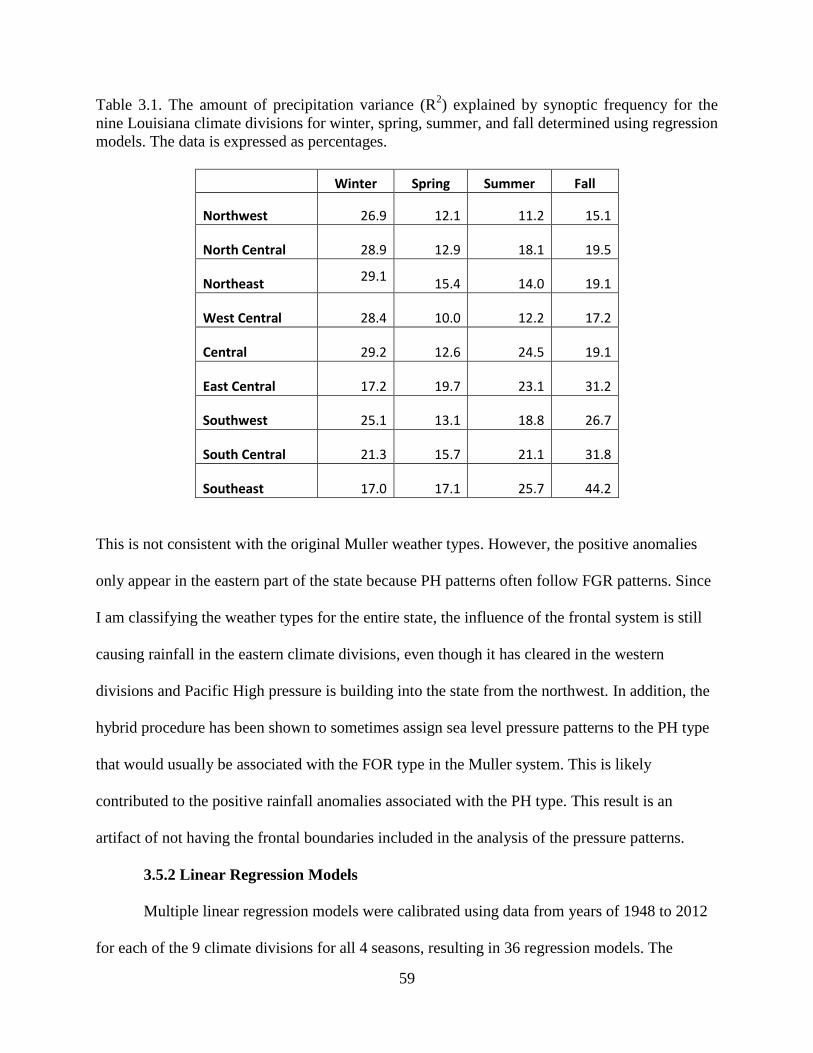
59

Table 3.1. The amount of precipitation variance (R2) explained by synoptic frequency for the

nine Louisiana climate divisions for winter, spring, summer, and fall determined using regression

models. The data is expressed as percentages.

Winter Spring Summer Fall

Northwest 26.9 12.1 11.2 15.1

North Central 28.9 12.9 18.1 19.5

Northeast 29.1

15.4 14.0 19.1

West Central 28.4 10.0 12.2 17.2

Central 29.2 12.6 24.5 19.1

East Central 17.2 19.7 23.1 31.2

Southwest 25.1 13.1 18.8 26.7

South Central 21.3 15.7 21.1 31.8

Southeast 17.0 17.1 25.7 44.2

This is not consistent with the original Muller weather types. However, the positive anomalies

only appear in the eastern part of the state because PH patterns often follow FGR patterns. Since

I am classifying the weather types for the entire state, the influence of the frontal system is still

causing rainfall in the eastern climate divisions, even though it has cleared in the western

divisions and Pacific High pressure is building into the state from the northwest. In addition, the

hybrid procedure has been shown to sometimes assign sea level pressure patterns to the PH type

that would usually be associated with the FOR type in the Muller system. This is likely

contributed to the positive rainfall anomalies associated with the PH type. This result is an

artifact of not having the frontal boundaries included in the analysis of the pressure patterns.

3.5.2 Linear Regression Models

Multiple linear regression models were calibrated using data from years of 1948 to 2012

for each of the 9 climate divisions for all 4 seasons, resulting in 36 regression models. The

60

adjusted R-squared of each multiple linear regression model measures the proportion of the

precipitation variance that can be explained by the predictor variables (the frequency of each

“wet” synoptic type). The explained variance ranges from 10% at the West Central climate

division in spring to 44.2% at the Southeast climate division in fall (Table 3.1). Averaged over

all climate divisions, the explained variance is approximately 25% for winter, 14% for spring,

19% for summer, and 25% for fall.

A residual analysis was applied to the regression models to test the assumptions of linear

regression. Normality was tested by plotting a histogram of the residuals for each model. The

residuals of each model appear approximately normal by visual inspection of the data plots;

however, they fail the Shapiro-Wilk test for normality. Small errors in normality do not greatly

affect the models, but large deviations from normality can affect confidence intervals

(Montgomery and Peck 1982). For the purposes of this analysis, we assume normality.

Regression is robust to normality errors and plots of the residuals ranked in increasing order

resemble straight lines, indicating approximate normality (Montgomery and Peck 1982). The

next assumption tested was heteroscadasticity. Visual examination of plots of the model

residuals vs. the precipitation estimates revealed some non-linearity in the models (Montgomery

and Peck 1982). For the purpose of this exploratory analysis, we assumed homoscedasticity, but

acknowledge that future work may need to incorporate non-linear models or attempt data

transformations to make the relationship between precipitation and synoptic type linear. The

normality and homoscedasticity plots can be found in Appendix B. The final assumption tested

was independence. The Durbin-Watson (D-W) test determined that the data were independent, as

each D-W statistic is near 2 (Table 3.1.).

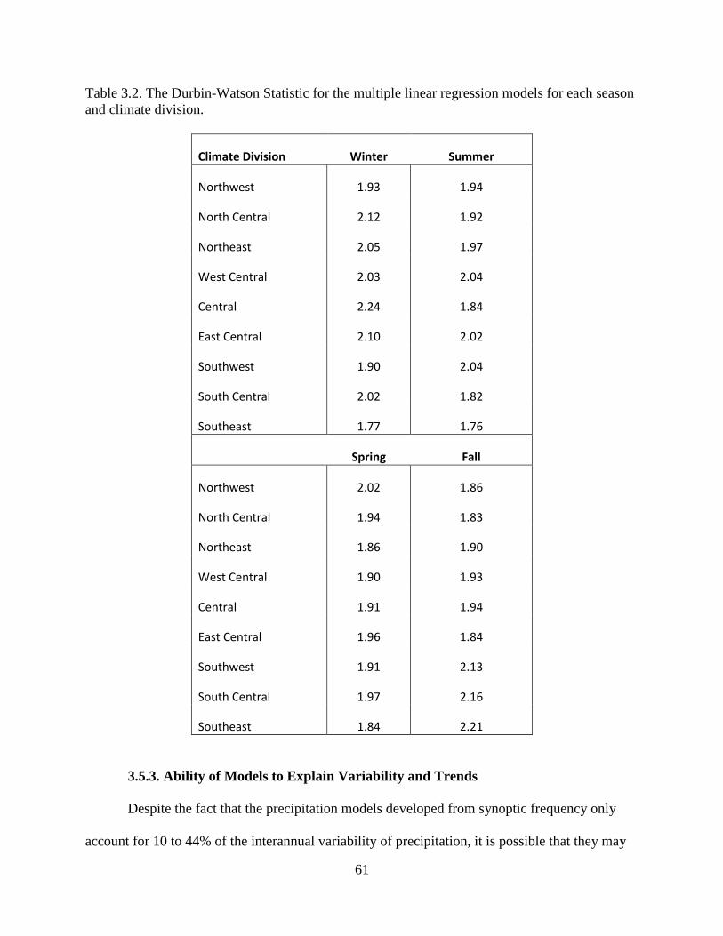
61

Table 3.2. The Durbin-Watson Statistic for the multiple linear regression models for each season

and climate division.

Climate Division Winter Summer

Northwest 1.93 1.94

North Central 2.12 1.92

Northeast 2.05 1.97

West Central 2.03 2.04

Central 2.24 1.84

East Central 2.10 2.02

Southwest 1.90 2.04

South Central 2.02 1.82

Southeast 1.77 1.76

Spring Fall

Northwest 2.02 1.86

North Central 1.94 1.83

Northeast 1.86 1.90

West Central 1.90 1.93

Central 1.91 1.94

East Central 1.96 1.84

Southwest 1.91 2.13

South Central 1.97 2.16

Southeast 1.84 2.21

3.5.3. Ability of Models to Explain Variability and Trends

Despite the fact that the precipitation models developed from synoptic frequency only

account for 10 to 44% of the interannual variability of precipitation, it is possible that they may

62

still be able to reasonably reproduce long-term (decadal-scale) variability and trends (Hanssen-

Bauer and Forland 1998). This is because, although the precipitation causes is irregularly

distributed, over longer time scales, the randomness of precipitation is smoothed out (Hanssen-

Bauer and Forland 1998). The smoothed regression modeled results versus observed

precipitation for each season and climate division can be found in Figure 3.6 – Figure 3.9. The

smoothed results represent decadal scale variability in the data.

The smoothed modeled versus precipitation series show, that during the winter and,

especially, the fall, the models account for most of the observed long-term precipitation features

in the Southeast climate division. However, during spring and summer, the models do not

adequately capture the observed variability and trends. In summer, weak pressure patterns set up

over the area, making it hard to distinguish between weather types. In addition, convective

rainfall often occurs during non-stormy weather types due to the intense surface heating that is

received during summer in this region. While the spring results are somewhat surprising and

deserve further investigation, the poor performance of the models is likely due to large amounts

of variability in precipitation amounts during stormy weather types in spring. Overall, the results

suggest that the models based on synoptic variability cannot sufficiently explain the interannual

variability of precipitation in Louisiana; however, they have the skills necessary to predict

longer-term variability and trends in winter and fall. It is likely that additional predictors are

necessary to model long-term precipitation variations in the spring and summer, and could

improve predictions in winter and fall as well.

63

Figure 3.6. Smoothed winter modeled and observed precipitation for each climate division from 1956 to 2005.

Northwest North Central Northeast

West Central Central East Central

Southwest South Central Southeast

64

Figure 3.7. Smoothed spring modeled and observed precipitation for each climate division from 1955 to 2005.




65

Figure 3.8. Smoothed summer modeled and observed precipitation for each climate division from 1955-2005.



Southwest Central South east South

66

Figure 3.9. Smoothed fall modeled and observed precipitation for each climate division from 1955 to 2005.




67

3.5.4 Limitations

This study is limited by a few different factors. First, and most importantly, the multiple

linear regression models used in the study depend on a linear relationship between each input

variable and the predictand. As determined in the residual analysis, this is not always the case

with the data used in this study. Future work should focus on finding a remedy for this weakness

by using data transformations or non- linear models. Additionally, this type of analysis is limited

by the irregularity of precipitation, making it hard to predict using a simple model. Additional

analyses could use models with more predictors or try use different Gaussian filters to detect

sources of regular variability in the region, such as the El Nino Southern Oscillation. Finally, the

models based on synoptic frequency are limited by the power of the synoptic classification

system to capture rainfall variability. There are some weaknesses in the hybrid classification

system, which are discussed in Chapter 2. Future improvements to the synoptic classification

system could improve the results of this study.

3.6 Summary and Conclusions

Precipitation in Louisiana varies considerably from year to year. To predict the future

effects of climate change, there is a need to better understand the controls of rainfall processes in

this region. This study was successful in identifying the synoptic patterns that are important to

precipitation generation in Louisiana, and the results were mostly consistent with the original

Muller weather typing system for Louisiana. However, it was determined that the variability of

synoptic types can only account for a small portion of the interannual rainfall variability in

Louisiana. This is likely due to a combination of reasons. The first is that precipitation is

irregularly distributed in time and space, and is therefore very difficult to predict on short time

scales. The second is that, in addition to synoptic atmospheric circulation, there are likely other

68

factors controlling rainfall in this region. Some possible additional predictors that could be

included in a precipitation model for this region are air temperature, sea surface temperature

(SST) and aerosol forcing.

On longer time scales, however, the predictability of the models improved for some

seasons. In winter and fall, the synoptic-based models do an adequate job of reproducing the

observed decadal variability and long-term precipitation trends. Therefore, synoptic-based

models may be a good candidate for determining future decadal precipitation variability and

trends from GCM outputs for these seasons. However, this does not provide any solutions for

spring and summer. While this study was an important first step to developing a statistical

downscaling model for Louisiana, additional research must be conducted to identify predictors

that can improve the predictability of the models for Louisiana precipitation.

3.7 References

Brisson, E., M. Demuzere, B. Kwakernaak & N. P. M. Van Lipzig (2011) Relations between

Atmospheric Circulation and Precipitation in Belgium. Meteorology and Atmospheric

Physics, 111, 27-39.

Diem, J. E. (2012) Influences of the Bermuda High and Atmospheric Moistening on Changes in

Summer Rainfall in the Atlanta, Georgia Region, USA. International Journal of

Climatology, 33, 160-172.

ESRI. 2008. How Zonal Statistics Work. In ArcGIS Desktop Help.





69




Finnis, J., J. Cassano, M. Holland, M. Serreze & P. Uotila (2009) Synoptically Forced

Hydroclimatology of Major Arctic Watersheds in General Circulation Models; Part 1:

The Mackenzie River Basin. International Journal of Climatology, 29, 1226-1243.

Goodess, C. M. & P. D. Jones (2002) Links between Circulation and Changes in the

Characteristics of Iberian Rainfall. International Journal of Climatology, 22, 1593-1615.

Guttman, N. B. & R. G. Quayle (1996) A Historical Perspective of U.S. Climate Divisions.

Bulletin of the American Meteorological Society, 77, 293-303.

Hanssen-Bauer, I. & E. J. Forland (1998) Long-Term Trends in Precipitation and Temperature in

the Norwegian Arctic: Can They Be Explained by Changes in Atmospheric Circulation

Patterns? Climate Research, 10, 143-153.

Higgins, R. W., J. E. Janowiak & Y.-P. Yao. 1996. A Gridded Hourly Precipitation Data Base

for the United States (1963-1993). In NCEP/Climate Prediction Center Atlas 1. National

Centers for Environmental Prediction.







IPCC. 2007. Climate Change 2007: The Physical Science Basis. Contribution of Working Group

I to the Fourth Assessment Report of the Intergovernmental Panel on Climate Change

[Solomon, S., D. Qin, M. Manning, Z. Chen, M. Marquis, K.B. Averyt, M. Tignor and

H.L. Miller (Eds.)]. Cambridge University Press, Cambridge, United Kingdom and New

York, Ny, USA, 996 Pp.

70

Kalnay, E., M. Kanamitsu, R. Kistler, W. Collins, D. Deaven, L. Gandin, M. Iredell, S. Saha, G.

White, J. Woollen, Y. Zhu, M. Chelliah, W. Ebisuzaki, W. Higgins, J. Janowiak, K. C.

Mo, C. Ropelewski, J. Wang, A. Leetmaa, R. Reynolds, R. Jenne & D. Joseph (1996)

The Ncep/Ncar 40-Year Reanalysis Project. Bulletin of the American Meteorological

Society, 77, 437-471.

Karl, T. R. & W. E. Riebsame (1989) The Impact of Decadal Fluctuations in Mean Precipitation

and Temperature on Runoff - a Sensitivity Study over the United States. Climatic

Change, 15, 423-447.

Keim, B. D. (1996) Spatial, Synoptic, and Seasonal Patterns of Heavy Rainfall in the

Southeastern United States. Physical Geography, 17, 313-328.

Keim, B. D. & G. E. Faiers (1996) Heavy Rainfall Distributions by Season in Louisiana:

Synoptic Interpretations and Quantile Estimates. Water Resources Bulletin, 32, 117-124.

Keim, B. D., R. Fontenot, C. Tebaldi & D. Shankman (2011) Hydroclimatology of the Us Gulf

Coast under Global Climate Change Scenarios. Physical Geography, 32, 561-582.

Kunkel, K. E., L. E. Stevens, S. E. Stevens, L. Sun, E. Janssen, D. Wuebbles, C. E. K. II, C. M.

Fuhrman, B. D. Keim, M. C. Kruk, A. Billiot, H. Needham, M. Shafer & J. G. Dobson.

2013. Regional Climate Trends and Scenarios for the U.S. National Climate Assessment

Part 2. Climate of the Southeast U.S. In NOAA Technical Report NESDIS 142-2.



McCabe, G. J. & R. A. Muller (1987) Synoptic Weather Types: An Index of Evaporation in

Southern Louisiana. Physical Geography, 8, 99-112.



Montgomery, D. C. & E. A. Peck. 1982. Introduction to Linear Regression Analysis. New York:

Wiley.



71



NOAA (2012) National Climatic Data Center, State of the Climate: Global Analysis for August

2012. http://www.ncdc.noaa.gov/sotc/global/2012/8 (last accessed October 31, 2012).

Rohli, R. V. & K. G. Henderson (1997) Winter Anticyclone Changes on the Central Gulf Coast

of the USA. International Journal of Climatology, 17, 1183-1193.

Trewartha, G. 1981. The Earth's Problem Climates. The University of Wisconsin Press.

USDM. 2012. U.S. Drought Monitor. National Drought Mitigation Center.


http://www.ncdc.noaa.gov/sotc/global/2012/8

72

CHAPTER 4. SUMMARY AND CONCLUSIONS

Automated synoptic classification has many applications for studying current and future

climate variability in a region. Louisiana is located in the South Central United States, a region

that is known for exhibiting large amounts of variability in surface weather, especially

precipitation. However, there are currently no widely accepted automated synoptic weather

classification systems for this region. The primary goals of this thesis were to 1) present an

automated synoptic weather type classification system for climate related studies in Louisiana

and 2) use the newly created synoptic classification system to determine the relationship between

synoptic type frequency and precipitation variability in Louisiana.

A new method of synoptic weather classification for Louisiana was presented in Chapter

2. The main objective of the new classification system was to avoid the weaknesses of both

manual and automated classification systems by creating a hybrid classification system based on

the Muller weather typing scheme for Louisiana. NCEP/NCAR Reanalysis sea level pressure

data from 12Z each day from 1981 – 2001 were typed using the Muller weather type archive, and

sea level pressure composites were generated for each Muller weather type. For the hybrid

procedure, these composites were used as seeds in a correlation algorithm to determine the most

appropriate weather type for each day. The Muller and hybrid types from 1981 – 2001 were

compared at daily, seasonal, and annual resolution. At a daily resolution, the hybrid types match

the Muller weather types at one or more location on 57 % of the days. For most of the weather

types there is significant agreement at the seasonal and annual resolutions. One sources of

discrepancy between the Muller and hybrid types was the inability of the hybrid procedure to

distinguish between tropical and baroclinic low pressure systems. The hybrid system also had

difficulty identifying the Muller FOR type because it does not have a strong surface pressure

73

signature. However, the goal of the procedure was not to replicate the Muller classification

system, but to create a new system that was automated and captured the essence of the Muller

weather types. The hybrid classification is homogenous within itself, and preliminary

investigations show it has value in describing the variability of surface weather in Louisiana. The

strengths of the automated hybrid system are its objectivity, speed, and reproducibility, making it

an advantageous candidate for long-term climate studies. It is also easily adaptable to GCM

output, opening up new applications for studying future synoptic climatology in the region.

The automated hybrid classification system presented in this study can be used for

seemingly endless applications in climate and climate impact research for Louisiana. This could

include updates to older studies that used the Muller classification systems (Muller and Jackson

1985, Faiers 1988, Faiers 1993, Faiers et al. 1994, Keim and Faiers 1996, McCabe and Muller

2002), as well as completely new studies, such as synoptic climatological investigations of future

climates using GCMs. In addition, future work related to this project could include developing

hybrid classification systems for other regions using the methodology presented in this study or

even expanding the classification developed here to include other parts of the South Central U.S.,

since the entire region experiences the similar synoptic patterns.

The newly developed automated classification system was used to study Louisiana

precipitation variability in Chapter 3. Using the hybrid weather classification system and gridded

daily precipitation data, wet synoptic types, or synoptic types that are associated with above

average daily rainfall, were identified for each climate division and season. The frequency of the

wet synoptic types was used to create a regression model to predict seasonal precipitation for

each climate division. The models developed from synoptic frequency only account for 10 –

44% of the interannual variability of precipitation in Louisiana. Averaged among all climate

74

divisions, the explained variance is 25% for winter, 14% for spring, 19% for summer, and 25%

for fall. Applying a smoothing technique to the modeled and observed rainfall data shows that

the predictability of the models is slightly improved on decadal time scales. However, more

research must be done to identify additional predictors before we can move forward with the

development of a statistical downscaling model for Louisiana. While the research presented in

this thesis was an important first step, the results suggest that a model based solely on synoptic

frequency cannot adequately describe the variability and trends in observed precipitation data for

all seasons. Therefore, the next step for this project will be to investigate other variables that will

improve the predictability of the models so that the project can move forward.

4.1 References








Keim, B. D. & G. E. Faiers (1996) Heavy Rainfall Distributions by Season in Louisiana:

Synoptic Interpretations and Quantile Estimates. Water Resources Bulletin, 32, 117-124.





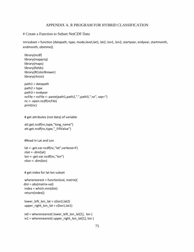
75

APPENDIX A. R PROGRAM FOR HYBRID CLASSIFICATION

# Create a Function to Subset NetCDF Data

nnrsubset = function (datapath, type, mode,level,lat1, lat2, lon1, lon2, startyear, endyear, startmonth,

endmonth, obstime){

library(ncdf) library(mapproj) library(maps) library(fields) library(RColorBrewer) library(chron)

path1 = datapath path2 = type path3 = endyear ncFile = ncFile <- paste(path1,path2,".",path3,".nc", sep='') nc <- open.ncdf(ncFile) print(nc)

# get attributes (not data) of variable

att.get.ncdf(nc,type,"long_name") att.get.ncdf(nc,type,"_FillValue")

#Read in Lat and Lon

lat <- get.var.ncdf(nc,"lat",verbose=F) nlat <- dim(lat) lon <- get.var.ncdf(nc,"lon") nlon <- dim(lon)

# get index for lat lon subset

wherenearest = function(val, matrix){ dist = abs(matrix-val) index = which.min(dist) return(index)} lower_left_lon_lat = c(lon2,lat2) upper_right_lon_lat = c(lon1,lat1) ix0 = wherenearest( lower_left_lon_lat[1], lon ) ix1 = wherenearest( upper_right_lon_lat[1], lon )

76

iy0 = wherenearest( lower_left_lon_lat[2], lat ) iy1 = wherenearest( upper_right_lon_lat[2], lat ) countx = ix1 - ix0 + 1 county = iy0 - iy1 + 1

# get time dimension

t <- get.var.ncdf(nc,"time") tunits <- att.get.ncdf(nc,"time","units")

# print t and tunits

head(t) tunits$value

# get "real" times

chron((t/24)-2,origin=c(month=1, day=1, year=0001)) time = chron((t/24)-2,origin=c(month=1, day=1, year=0001)) # get data subset

if (type == "hgt"){ x = length(t) subset = get.var.ncdf(nc,type, start = c(ix0,iy1,level,1), count = c(countx,county,1,x)) dim(subset)} else if (type == "slp"){x = length(t) subset = get.var.ncdf(nc,type, start = c(ix0,iy1,1), count = c(countx,county,x)) dim(subset)} #####################################################################################

# Create a matrix of Lat/Lon

lon = rep(seq(lon2, lon1, by = 2.5), each = county) lat = rev(rep(seq(lat2,lat1,by = 2.5), countx)) tMat <- matrix(c(lon,lat),nrow=length(lat),ncol=2)

# Put data in Loc Dataframe

names = time colnames = c("hours", "month", "year", seq(1, length(lat))) Loc = data.frame(row.names = names, hours(time), months(time), years(time))

77

for (j in 1:countx){ for (k in 1:county){ Loc = cbind(Loc,subset[j,k,])}} names(Loc) = colnames

#####################################################################################

# Subset the remaining data y = c(startyear:(endyear-1)) y = rev(y) y = as.numeric(y) path1 = datapath path2 = type nc <- open.ncdf(ncFile) print(nc) for (i in y){ ncFile = ncFile <- paste(path1,path2,".",i,".nc", sep='') nc <- open.ncdf(ncFile) print(nc) # get attributes (not data) of slp att.get.ncdf(nc,type,"long_name") att.get.ncdf(nc,type,"_FillValue") #Read in Lat and Lon lat <- get.var.ncdf(nc,"lat",verbose=F) nlat <- dim(lat) lon <- get.var.ncdf(nc,"lon") nlon <- dim(lon) # get index for lat lon subset wherenearest = function(val, matrix){ dist = abs(matrix-val) index = which.min(dist) return(index)} lower_left_lon_lat = c(lon2,lat2) upper_right_lon_lat = c(lon1,lat1)

78

ix0 = wherenearest( lower_left_lon_lat[1], lon ) ix1 = wherenearest( upper_right_lon_lat[1], lon ) iy0 = wherenearest( lower_left_lon_lat[2], lat ) iy1 = wherenearest( upper_right_lon_lat[2], lat ) countx = ix1 - ix0 + 1 county = iy0 - iy1 + 1 #read in levels #lev <- get.var.ncdf(nc,"level") #nlev <- dim(lev) library(chron) # get time dimension t <- get.var.ncdf(nc,"time") tunits <- att.get.ncdf(nc,"time","units") # print t and tunits head(t) tunits$value # get "real" times chron((t/24)-2,origin=c(month=1, day=1, year=0001)) time = chron((t/24)-2,origin=c(month=1, day=1, year=0001)) # get data subset if (type == "hgt"){ x = length(t) subset = get.var.ncdf(nc,type, start = c(ix0,iy1,level,1), count = c(countx,county,1,x)) dim(subset)} else if (type == "slp"){x = length(t) subset = get.var.ncdf(nc,type, start = c(ix0,iy1,1), count = c(countx,county,x)) dim(subset)} # Put data in Loc Dataframe lon = rep(seq(lon2, lon1, by = 2.5), each = county)

79

lat = rev(rep(seq(lat2,lat1,by = 2.5), countx)) names = time colnames = c("hours", "month", "year", seq(1,length(lat))) Loc2 = data.frame(row.names = names, hours(time), months(time), years(time)) for (j in 1:countx){ for (k in 1:county){ Loc2 = cbind(Loc2,subset[j,k,])}} names(Loc2) = colnames Loc = rbind(Loc,Loc2) } ##################################################################################### #Subset data to include only observation time and months of input twelve = subset(Loc, hours == obstime) month = c("Jan", "Feb", "Mar", "Apr", "May", "Jun", "Jul", "Aug", "Sep", "Oct", "Nov", "Dec") summertwelve = data.frame() for (i in c(startmonth:endmonth)){ monthname = month[i] monthtwelve = subset(twelve, month == monthname) summertwelve = rbind(summertwelve, monthtwelve)} timedetails = summertwelve[, 1:3] final = summertwelve[, 4:(length(lat)+3)] final = as.matrix(final) if (mode == "S"){ list = list("subset" = final, "locations" = tMat, "timedetails" = timedetails) } else if (mode == "T"){ list = list("subset" = t(final), "locations" = tMat, "timedetails" = timedetails) }

80

return(list)}

##############################################################################

# Preform Hybrid Classification

# Extract sea level pressure grids from nnrsubset list

subset = nrrsubset$subset

# Standardize sea level pressure grids

subset_standard = t(subset) subset_standard = scale(subset_standard, center = TRUE, scale = TRUE) subset_standard = t(subset_standard) # Read in Muller Weather types from excel file and assign to sea level pressure grids file2 = "J:/Thesis/Muller Types/1981-2001 Procedure/Muller_Types_81_01_Non_Transition.csv" Muller = read.csv(file2,header = TRUE, sep = ",") Muller = cbind(Muller, subset_standard) # Aggregate by Muller Type to calculate mean grids for each Muller_mean = aggregate(Muller, by = list(Muller$Baton.Rouge.6Z), FUN = mean) Muller_mean = Muller_mean[,6:148] Muller_mean = Muller_mean[2:9,] # Calculate sum of squares between each grid and each mean grid

kirch = data.frame(row.names = rownames(subset1))

for (i in 1:8){ grid = matrix(as.numeric(rep(Muller_mean[i,], 7670)), nrow = 7670, byrow = TRUE) grid = grid - subset_standard squares = grid^2 sumofsquares = rowSums(squares) kirch = cbind(kirch, sumofsquares)} # Find minimum kirch score and assign a weather type to each grid

kirch = kirch * -1 kirch$types = max.col(kirch) types2 = data.frame(rownames(kirch), kirch$types) write.csv(hybridtypes, file = "Hybrid_Types.csv")

81

APPENDIX B. RESIDUAL ANALYSIS

Figure A.1. Histogram of Winter Regression Model Residuals for the A) Northwest B) North

Central C) Northeast D) West Central E) Central F) East Central G) Southwest H) South Central

I) Southeast Climate Divisions.

82

Figure A.2. Histogram of Spring Regression Model Residuals for the A) Northwest B) North



83

Figure A.3. Histogram of Summer Regression Model Residuals for the A) Northwest B) North



84

Figure A.4. Histogram of Fall Regression Model Residuals for the A) Northwest B) North



85

Figure A.5. Winter Regression Model Residuals vs. Winter Precipitation Estimates for the A)

Northwest B) North Central C) Northeast D) West Central E) Central F) East Central G)

Southwest H) South Central I) Southeast Climate Divisions.

86

Figure A.6. Spring Regression Model Residuals vs. Spring Precipitation Estimates for the A)



87

Figure A.7. Summer Regression Model Residuals vs. Summer Precipitation Estimates for the A)



88

Figure A.8. Fall Regression Model Residuals vs. Fall Precipitation Estimates for the A)



89

THE VITA

Amanda Billiot, a native of Southeast Louisiana, received her bachelor’s degree in

Meteorology at the University of South Alabama in 2011. She entered graduate school in the

Department of Anthropology and Geography at Louisiana State University shortly thereafter.

Amanda plans to begin work on her doctorate upon graduation.

a hybrid procedure for classifying synoptic weather types

Documents