a history of satisﬁability - john francogauss.ececs.uc.edu/sat/articles/faia185-0003.pdf · with...

�

�

“p01c01˙his” — 2008/11/20 — 10:11 — page 3 — #3�

�

�

�

�

�

Handbook of Satisfiability

Armin Biere, Marijn Heule, Hans van Maaren and Toby Walsh (Eds.)

IOS Press, 2009

c© 2009 John Franco and John Martin and IOS Press. All rights reserved.

3

Chapter 1

A History of SatisfiabilityJohn Franco and John Martin

with sections contributed by Miguel Anjos, Holger Hoos, Hans Kleine Buning,

Ewald Speckenmeyer, Alasdair Urquhart, and Hantao Zhang

1.1. Preface: the concept of satisfiability

Interest in Satisfiability is expanding for a variety of reasons, not in the leastbecause nowadays more problems are being solved faster by SAT solvers thanother means. This is probably because Satisfiability stands at the crossroadsof logic, graph theory, computer science, computer engineering, and operationsresearch. Thus, many problems originating in one of these fields typically havemultiple translations to Satisfiability and there exist many mathematical toolsavailable to the SAT solver to assist in solving them with improved performance.Because of the strong links to so many fields, especially logic, the history ofSatisfiability can best be understood as it unfolds with respect to its logic roots.Thus, in addition to time-lining events specific to Satisfiability, the chapter followsthe presence of Satisfiability in logic as it was developed to model human thoughtand scientific reasoning through its use in computer design and now as modelingtool for solving a variety of practical problems. In order to succeed in this, wemust introduce many ideas that have arisen during numerous attempts to reasonwith logic and this requires some terminology and perspective that has developedover the past two millennia. It is the purpose of this preface to prepare thereader with this information so as to make the remainder of the chapter moreunderstandable and enlightening.

Logic is about validity and consistency. The two ideas are interdefinable ifwe make use of negation (¬): the argument from p1, . . . , pn to q is valid if andonly if the set {p1, . . . , pn,¬q} is inconsistent. Thus, validity and consistency arereally two ways of looking at the same thing and each may be described in termsof syntax or semantics.

The syntactic approach gives rise to proof theory. Syntax is restricted todefinitions that refer to the syntactic form (that is, grammatical structure) of thesentences in question. In proof theory the term used for the syntactic versionof validity is derivability. Proofs are derived with respect to an axiom system

which is defined syntactically as consisting of a set of axioms with a specifiedgrammatical form and a set of inference rules that sanction proof steps with

doi:10.3233/978-1-58603-929-5-3

�

�

“p01c01˙his” — 2008/11/20 — 10:11 — page 4 — #4�

�

�

�

�

�

4 Chapter 1. A History of Satisfiability

specified grammatical forms. Given an axiom system, derivability is defined asfollows: q is derivable from p1, . . . , pn (in symbols, p1, . . . , pn � q) if and only ifthere is a proof in the axiom system of q (derivable) from p1, . . . , pn. Becausethe axioms and rules are defined syntactically, so is the notion of derivability.The syntactic version of consistency is simply called consistency, and is definedas follows: {p1, . . . , pn} is consistent if and only if it is not possible to derive acontradiction from {p1, . . . , pn}. It follows that {p1, . . . , pn} is inconsistent if andonly if there is some contradiction q ∧ ¬q such that {p1, . . . , pn} � q ∧ ¬q. Sincederivability has a definition that only makes reference to the syntactic shapes, andsince consistency is defined in terms of derivability, it follows that consistency toois a syntactic concept, and is defined ultimately in terms of grammatical formalone. The inference rules of axiom systems, moreover, are always chosen so thatderivability and consistency are interdefinable: that is, p1, . . . , pn � q if and onlyif {p1, . . . , pn,¬q} is inconsistent.

The semantic approach gives rise to model theory. Semantics studies theway sentences relate to “the world.” Truth is the central concept in semanticsbecause a sentence is said to be true if it “corresponds to the world.” The conceptof algebraic structure is used to make precise the meaning of “corresponds to theworld.”

An algebraic structure, or simply structure, consists of a non-empty set ofobjects existing in the world w, called the domain and denoted below by D, anda function, called an interpretation and denoted below by R, that assigns to eachconstant an entity in D, to each predicate a relation among entities in D, and toeach functor a function among entities in D. A sentence p is said to be true in w

if the entities chosen as the interpretations of the sentence’s terms and functorsstand to the relations chosen as the interpretation of the sentence’s predicates.We denote a structure by 〈D,R〉. Below we sometimes use A to stand for 〈D,R〉

by writing A = 〈D,R〉. A more traditional, algebraic notation for structure isused in Section 1.6. We will speak of formulas instead of sentences to allow forthe possibility that a sentence contains free variables. The customary notation isto use A |= p to say p is true in the structure A.

The semantic versions of validity and consistency are defined in terms of theconcept of structure. In model theory validity is just called validity. Intuitively,an argument is valid if whenever the premises are true, so is the conclusion. Moreprecisely, the argument from p1, . . . , pn to q is valid (in symbols, p1, . . . , pn |= q)if and only if, for all structures A, if A |= p1, . . . ,A |= pn, then A |= q.

We are now ready to encounter, for the first time, satisfiability, the centralconcept of this handbook. Satisfiability is the semantic version of consistency.A set of formulas is said to be satisfiable if there is some structure in which allits component formulas are true: that is, {p1, . . . , pn} is satisfiable if and only if,for some A, A |= p1 and . . . and A |= pn. It follows from the definitions thatvalidity and satisfiability are mutually definable: p1, . . . , pn |= q if and only if{p1, . . . , pn,¬q} is unsatisfiable.

Although the syntactic and semantic versions of validity and consistency -namely derivability and consistency, on the one hand, and validity and satisfia-bility, on the other - have different kinds of definitions, the concepts from the twobranches of logic are systematically related. As will be seen later, for the lan-

�

�

“p01c01˙his” — 2008/11/20 — 10:11 — page 5 — #5�

�

�

�

�

�

Chapter 1. A History of Satisfiability 5

guages studied in logic it is possible to devise axiom systems in such a way thatthe syntactic and semantic concepts match up so as to coincide exactly. Deriv-ability coincides with validity (i.e. p1, . . . , pn � q if and only if p1, . . . , pn |= q),and consistency coincides with satisfiability (i.e. {p1, . . . , pn} is consistent if andonly if {p1, . . . , pn} is satisfiable). Such an axiom system is said to be complete.

We have now located satisfiability, the subject of this handbook, in thebroader geography made up of logic’s basic ideas. Logic is about both valid-ity and consistency, which are interdefinable in two different ways, one syntac-tic and one semantic. Among these another name for the semantic version ofconsistency is satisfiability. Moreover, when the language possesses a completeaxiom system, as it normally does in logic, satisfiability also coincides exactlywith syntactic consistency. Because of these correspondences, satisfiability maythen be used to “characterize” validity (because p1, . . . , pn |= q if and only if{p1, . . . , pn,¬q} is unsatisfiable) and derivability (because p1, . . . , pn � q if andonly if {p1, . . . , pn,¬q} is unsatisfiable).

There is a further pair of basic logical ideas closely related to satisfiability:necessity and possibility. Traditionally, a sentence is said to be necessary (ornecessarily true) if it is true in all possible worlds, and possible (or possibly true)if it is true in at least one possible world. If we understand a possible world tobe a structure, possibility turns out to be just another name for satisfiability. Apossible truth is just one that is satisfiable. In logic, the technical name for anecessary formula is logical truth: p is defined to be a logical truth (in symbols,|= p) if and only if, for all A, A |= p. (In sentential logic a logical truth is called atautology.) Moreover, necessary and possible are predicates of the metalanguage(the language of logical theory) because they are used to describe sentences inthe “object” language (the language that refers to entities in the world that isthe object of investigation in logical theory).

There is one further twist. In the concept of consistency we have alreadythe syntactic version of satisfiability. There is also a syntactic version of a logicaltruth, namely a theorem-in-an-axiom-system. We say p is a theorem of the system(in symbols |= p) if and only if p is derivable from the axioms alone. In a completesystem, theorem-hood and logical truth coincide: � p if and only if |= p. Thus,in logical truth and theorem-hood we encounter yet another pair of syntactic andsemantic concepts that, although they have quite different sorts of definitions,nevertheless coincide exactly. Moreover, a formula is necessary if it is not possiblynot true. In other words, |= p if and only if it is not the case that p is unsatisfiable.Therefore, satisfiability, theorem-hood, logical truths and necessities are mutually“characterizable.”

This review shows how closely related satisfiability is to the central conceptsof logic. Indeed, relative to a complete axiom system, satisfiability may be usedto define, and may be defined by, the other basic concepts of the field - valid-ity, derivability, consistency, necessity, possibility, logical truth, tautology, andtheorem-hood.

However, although we have taken the trouble to clearly delineate the distinc-tion between syntax and semantics in this section, it took over 2000 years beforethis was clearly enunciated by Tarski in the 1930s. Therefore, the formal notionof satisfiability was absent until then, even though it was informally understood

�

�

“p01c01˙his” — 2008/11/20 — 10:11 — page 6 — #6�

�

�

�

�

�


since Aristotle.The early history of satisfiability, which will be sketched in the next sections,

is the story of the gradual enrichment of languages from very simple languagesthat talk about crude physical objects and their properties, to quite sophisticatedlanguages that can describe the properties of complex structures and computerprograms. For all of these languages, the core concepts of logic apply. They allhave a syntax with constants that stand for entities and with predicates thatstand for relations. They all have sentences that are true or false relative topossible worlds. They all have arguments that are valid or invalid. They all havelogical truths that hold in every structure. They all have sets that are satisfiableand others that are unsatisfiable. For all of them, logicians have attempted todevise complete axiom systems to provide syntactic equivalents that capture, inthe set of theorems, exactly the set of logical truths, that replicate in syntacticderivations exactly the valid arguments, and provide derivations of contradictionsfrom every unsatisfiable set. We shall even find examples in these early systemsof attempts to define decision procedures for logical concepts. As we shall see, inall these efforts the concept of satisfiability is central.

1.2. The ancients

It was in Athens that logic as a science was invented by Aristotle (384-322 B.C.).In a series of books called the Organon, he laid the foundation that was to guidethe field for the next 2000 years. The logical system he invented, which is calledthe syllogistic or categorical logic, uses a simple syntax limited to subject-predicatesentences.

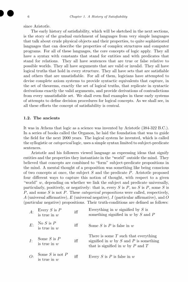
Aristotle and his followers viewed language as expressing ideas that signifyentities and the properties they instantiate in the “world” outside the mind. Theybelieved that concepts are combined to “form” subject-predicate propositions inthe mind. A mental thought of a proposition was something like being consciousof two concepts at once, the subject S and the predicate P . Aristotle proposedfour different ways to capture this notion of thought, with respect to a given“world” w, depending on whether we link the subject and predicate universally,particularly, positively, or negatively: that is, every S is P , no S is P , some S isP , and some S is not P . These categorical propositions were called, respectively,A (universal affirmative), E (universal negative), I (particular affirmative), and O

(particular negative) propositions. Their truth-conditions are defined as follows:

A:Every S is P

is true in wiff

Everything in w signified by S issomething signified in w by S and P

E:No S is P

is true in wiff Some S is P is false in w

I:Some S is P

is true in wiff

There is some T such that everythingsignified in w by S and P is somethingthat is signified in w by P and T

O:Some S is not P

is true in wiff Every S is P is false in w

�

�

“p01c01˙his” — 2008/11/20 — 10:11 — page 7 — #7�

�

�

�

�

�


These propositions have the following counterparts in set theory:

S ⊆ P iff S = S ∩ P

S ∩ P = ∅ iff ¬(S ∩ P = ∅)S ∩ P = ∅ iff ∃T : S ∩ P = P ∩ T

S ∩ P = ∅ iff ¬(S = S ∩ P )

The resulting logic is two-valued: every proposition is true or false. It is truethat Aristotle doubted the universality of this bivalence. In a famous discussionof so-called future contingent sentences, such as “there will be a sea battle to-morrow,” he pointed out that a sentence like this, which is in the future tense, isnot now determined to be either true or false. In modern terms such a sentence“lacks a truth-value” or receives a third truth-value. In classical logic, however,the law of excluded middle (commonly known as tertium non datur), that is, p

or not p is always true, was always assumed.Unlike modern logicians who accept the empty set, classical logicians as-

sumed, as a condition for truth, that a proposition’s concepts must signify atleast one existing thing. Thus, the definitions above work only if T is a non-empty set. It follows that A and E propositions cannot both be true (they arecalled contraries), and that I and O propositions cannot both be false. The def-initions are formulated in terms of identity because doing so allowed logiciansto think of mental proposition formulation as a process of one-to-one conceptcomparison, a task that conciousness seemed perfectly capable of doing.

In this theory of mental language we have encountered the first theory ofsatisfiability. A proposition is satisfiable (or possible, as traditional logicianswould say) if there is some world in which it is true. A consistent proposition isone that is satisfiable. Some propositions were recognized as necessary, or alwaystrue, for example: every S is S.

Satisfiability can be used to show that propositions p1, . . . , pn do not logicallyimply q: one only needs to show that there is some assignment of concepts to theterms so that all the propositions in {p1, . . . , pn,¬q} come out true. For example,consider the statement:

(some M is A ∧ some C is A) → every M is C.

Aristotle would show this statement is false by replacing the letters with familiarterms to obtain the requisite truth values: some man is an animal and some cowis an animal are both true, but every man is a cow is false. In modern terms, wesay the set

{ some M is A, some C is A,¬( every M is C ) }

is satisfiable.The means to deduce (that is, provide a valid argument) was built upon

syllogisms, using what is essentially a complete axiom system for any conditional(p1, . . . , pn) → q in which p1, . . . , pn, and q are categorical propositions [Mar97].A syllogism is defined as a conditional (p∧q)→ r in which p,q, and r are A, E, I,or O propositions. To show that propositions are valid, that is (p1∧ . . .∧pn)→ q,

�

�

“p01c01˙his” — 2008/11/20 — 10:11 — page 8 — #8�

�

�

�

�

�


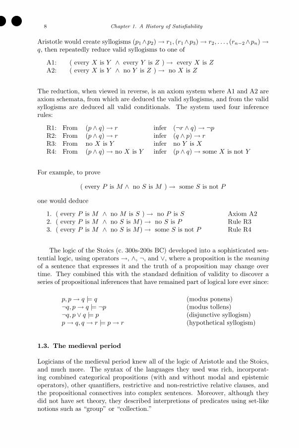
Aristotle would create syllogisms (p1∧p2)→ r1, (r1∧p3)→ r2, . . . , (rn−2∧pn)→q, then repeatedly reduce valid syllogisms to one of

A1: ( every X is Y ∧ every Y is Z )→ every X is Z

A2: ( every X is Y ∧ no Y is Z )→ no X is Z

The reduction, when viewed in reverse, is an axiom system where A1 and A2 areaxiom schemata, from which are deduced the valid syllogisms, and from the validsyllogisms are deduced all valid conditionals. The system used four inferencerules:

R1: From (p ∧ q)→ r infer (¬r ∧ q)→ ¬p

R2: From (p ∧ q)→ r infer (q ∧ p)→ r

R3: From no X is Y infer no Y is X

R4: From (p ∧ q)→ no X is Y infer (p ∧ q)→ some X is not Y

For example, to prove

( every P is M ∧ no S is M )→ some S is not P

one would deduce

1. ( every P is M ∧ no M is S )→ no P is S Axiom A22. ( every P is M ∧ no S is M)→ no S is P Rule R33. ( every P is M ∧ no S is M)→ some S is not P Rule R4

The logic of the Stoics (c. 300s-200s BC) developed into a sophisticated sen-tential logic, using operators →, ∧, ¬, and ∨, where a proposition is the meaning

of a sentence that expresses it and the truth of a proposition may change overtime. They combined this with the standard definition of validity to discover aseries of propositional inferences that have remained part of logical lore ever since:

p, p→ q |= q (modus ponens)¬q, p→ q |= ¬p (modus tollens)¬q, p ∨ q |= p (disjunctive syllogism)p→ q, q → r |= p→ r (hypothetical syllogism)

1.3. The medieval period

Logicians of the medieval period knew all of the logic of Aristotle and the Stoics,and much more. The syntax of the languages they used was rich, incorporat-ing combined categorical propositions (with and without modal and epistemicoperators), other quantifiers, restrictive and non-restrictive relative clauses, andthe propositional connectives into complex sentences. Moreover, although theydid not have set theory, they described interpretions of predicates using set-likenotions such as “group” or “collection.”

�

�

“p01c01˙his” — 2008/11/20 — 10:11 — page 9 — #9�

�

�

�

�

�


The development of concepts open to decision by an effective process (suchas a mechanical process) was actually an important goal of early modern logic,although it was not formulated in those terms. A goal of symbolic logic is to makeepistemically transparent judgments that a formula is a theorem of an axiomsystem or is deducible within an axiom system. An effective process ensures thistransparency because it is possible to know with relative certainty that each stagein the process is properly carried out.

The work of Ramon Lull (1232-1315) was influential beyond the medievalperiod. He devised the first system of logic based on diagrams expressing truthand rotating wheels to achieve some form of deduction. It had similarities toimportant later work, for example Venn circles, and greatly influenced Leibniz inhis quest for a system of deduction that would be universal.

1.4. The renaissance

In the 17th century Descartes and Leibniz began to understand the power ofapplying algebra to scientific reasoning. To this end, Leibniz devised a languagethat could be used to talk about either ideas or the world. He thought, like wedo, that sets stand to one another in the subset relation ⊆, and that a new setcan be formed by intersection ∩. He also thought that concepts can be combinedby definitions: for example the concepts animal and rational can be combined toform the concept rational+animal, which is the definition of the concept man, andthe concept animal would then be a “part” of the concept man. The operator ,called concept inclusion, was introduced to express this notion: thus, animal man.

Leibniz worked out dual Boolean interpretations of syllogistic propositionsjoined with the propositional connectives. The first (intensional) interpretationassigns terms to “concepts” within a structure of concepts ordered by andorganized by operations that we would call meet and join. The dual (extensional)interpretation is over a Boolean algebra of sets.

The logical operations of multiplication, addition, negation, identity, class in-clusion, and the null class were known at this time, well before Boole, but Leibnizpublished nothing on his ideas related to formal logic. In addition to his logicis rooted in the operators of identity (=), and a conjunction-like operator (⊕)called real addition, which obeys the following:

t⊕ t = t (idempotency)t⊕ t

′ = t′ ⊕ t (commutativity)t⊕ (t′ ⊕ t′′) = (t⊕ t′)⊕ t′′ (associativity)

where t, t′, and t′′ are terms representing substance or ideas. The following, Leib-niz’s equivalence, shows the tie between set inclusion and real addition that is thebasis of his logics.

t t′ if and only if t⊕ t′ = t′

Although Leibniz’s system is simplistic and ultimately implausible as an accountof science, he came very close to defining with modern rigor complete axiomsystems for well-defined formal languages that also possessed decision procedures

�

�

“p01c01˙his” — 2008/11/20 — 10:11 — page 10 — #10�

�

�

�

�

�


for identifying the sentences satisfied in every interpretation. It would be 250years before modern logic accomplished the same for its more complex languages.His vision is relevant to modern times in other ways too. As examples, he inventedbinary arithmetic, and his calculus ratiocinator is regarded by some as a formalinference engine, its use not unlike that of a computer programming language,and by others as referring to a “calculating machine” that was a forerunner tothe modern digital computer. In fact, Leibniz constructed a machine, called aStepped Reckoner, for mathematical calculations. Yet, at this point in history,the notion of satisfiability still had not been enunciated.

1.5. The first logic machine

According to Gardner [Gar58] the first logic machine, that is the first machine ableto solve problems in formal logic (in this case syllogisms), was invented by CharlesStanhope, 3rd Earl Stanhope (1753-1816). It employed methods similar to Venncircles (Section 1.6) and therefore can in some sense be regarded as Boolean.However, it was also able to go beyond traditional syllogisms to solve numericalsyllogisms such as the following: 8 of 10 pigeons are in holes, and 4 of the 10pigeons are white (conclude at least 2 holes have white pigeons). See [Gar58] fordetails.

1.6. Boolean algebra

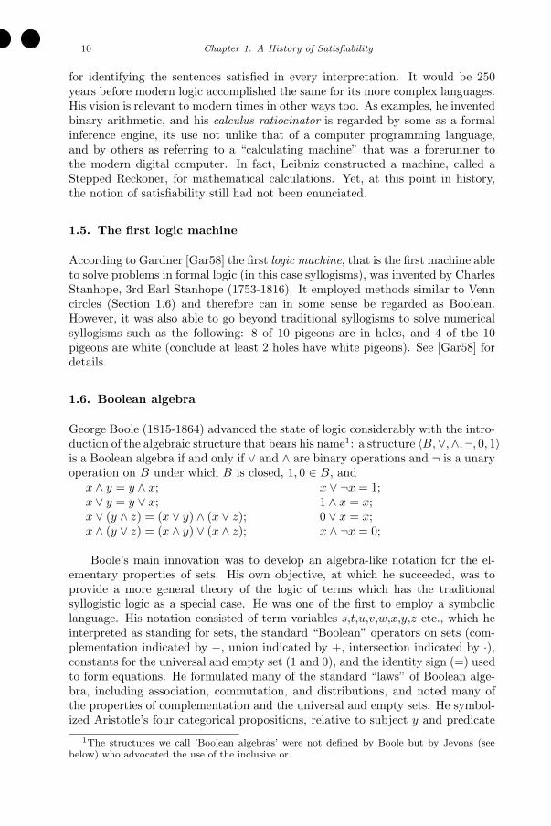
George Boole (1815-1864) advanced the state of logic considerably with the intro-duction of the algebraic structure that bears his name1: a structure 〈B,∨,∧,¬, 0, 1〉is a Boolean algebra if and only if ∨ and ∧ are binary operations and ¬ is a unaryoperation on B under which B is closed, 1, 0 ∈ B, and

x ∧ y = y ∧ x; x ∨ ¬x = 1;x ∨ y = y ∨ x; 1 ∧ x = x;x ∨ (y ∧ z) = (x ∨ y) ∧ (x ∨ z); 0 ∨ x = x;x ∧ (y ∨ z) = (x ∧ y) ∨ (x ∧ z); x ∧ ¬x = 0;

Boole’s main innovation was to develop an algebra-like notation for the el-ementary properties of sets. His own objective, at which he succeeded, was toprovide a more general theory of the logic of terms which has the traditionalsyllogistic logic as a special case. He was one of the first to employ a symboliclanguage. His notation consisted of term variables s,t,u,v,w,x,y,z etc., which heinterpreted as standing for sets, the standard “Boolean” operators on sets (com-plementation indicated by −, union indicated by +, intersection indicated by ·),constants for the universal and empty set (1 and 0), and the identity sign (=) usedto form equations. He formulated many of the standard “laws” of Boolean alge-bra, including association, commutation, and distributions, and noted many ofthe properties of complementation and the universal and empty sets. He symbol-ized Aristotle’s four categorical propositions, relative to subject y and predicate

1The structures we call ’Boolean algebras’ were not defined by Boole but by Jevons (see

below) who advocated the use of the inclusive or.

�

�

“p01c01˙his” — 2008/11/20 — 10:11 — page 11 — #11�

�

�

�

�

�


x, by giving names of convenience V (V = 0) to sets that intersect appropriatelywith y and x forming subsets:

Boole Sets

Every x is y: x = x · y x ⊆ y

No x is y: 0 = x · y x ⊆ y

Some x is y: V = V · x · y x ∩ y = ∅Some x is not y: V = V · x · (1− y) x ∩ y = ∅

Boole was not interested in axiom systems, but in the theory of inference. Inhis system it could be shown that the argument from p1, . . . , pn to q is valid (i.e.p1, . . . , pn |= q) by deriving the equation q from equations p1, . . . , pn by applyingrules of inference, which were essentially cases of algebraic substitution.

However, Boole’s algebras needed a boost to advance their acceptance. Gard-ner [Gar58] cites John Venn (1834-1923) and William Stanley Jevons (1835-1882)as two significant contributors to this task. Jevons regarded Boole’s work asthe greatest advance since Aristotle but saw some flaws that he believed keptit from significantly influencing logicians of the day, particularly that it was toomathematical. To fix this he introduced, in the 1860’s, the “method of indirectinference” which is an application of reductio ad absurdum to Boolean logic. Forexample, to handle ‘All x is y’ and ‘No y is z’ Jevons would write all possible“class explanations” as triples

xyz, xy¬z, x¬yz, x¬y¬z, ¬xyz, ¬xy¬z, ¬x¬yz, ¬x¬y¬z,

where the first represents objects in classes x, y, and z, the second representsobjects in classes x and y but not in z, and so on2. Then some of these tripleswould be eliminated by the premises which imply they are empty. Thus, x¬yz

and x¬y¬z are eliminated by ‘All x is y’ and xyz and ¬xyz are eliminated by‘No y is z’. Since no remaining triples contain both x and z, one can conclude‘No x is z’ and ‘No z is x’.

Although Jevons’ system is powerful it has problems with some statements:for example, ‘Some x is y’ cannot eliminate any of the triples xyz and xy¬z sinceat least one but maybe both represent valid explanations. Another problem isthe exponential growth of terms, although this did not seem to be a problem atthe time3. Although the reader can see x, y and z taking truth values 0 or 1,Jevons did not appreciate the fact that truth-value logic would eventually replaceclass logic and his attention was given only to the latter. He did build a logicmachine (called a “logic piano” due to its use of keys) that can solve five termproblems [Jev70] (1870). The reader is refered to [Gar58] for details.

What really brought clarity to Boolean logic, though, was the contributionof Venn [Ven80] (1880) of which the reader is almost certainly acquainted sinceit touches several fields beyond logic. We quote the elegantly stated passageof [Gar58] explaining the importance of this work:

2Jevons did not use ¬ but lower and upper case letters to distinguish inclusion and exclusion.3Nevertheless, Jevons came up with some labor saving devices such as inked rubber stamps

to avoid having to list all possibilities at the outset of a problem.

�

�

“p01c01˙his” — 2008/11/20 — 10:11 — page 12 — #12�

�

�

�

�

�


It was of course the development of an adequate symbolic notation that reduced the

syllogism to triviality and rendered obsolete all the quasi-syllogisms that had been so

painfully and exhaustively analyzed by the 19th century logicians. At the same time

many a controversy that once seemed so important no longer seemed so. ... Perhaps

one reason why these old issues faded so quickly was that, shortly after Boole laid

the foundations for an algebraic notation, John Venn came forth with an ingenious

improvement to Euler’s circles4. The result was a diagrammatic method so perfectly

isomorphic with the Boolean class algebra, and picturing the structure of class logic

with such visual clarity, that even a nonmathematically minded philosopher could “see”

what the new logic was all about.

As an example, draw a circle each for x, y, and z and overlap them so all possibleintersections are visible. A point inside circle x corresponds to x and a pointoutside circle x corresponds to ¬x and so on. Thus a point inside circles x

and y but outside circle z corresponds to Jevons’ xy¬z triple. Reasoning aboutsyllogisms follows Jevons as above except that the case ‘Some x is y’ is handledby placing a mark on the z circle in the region representing xy which means itis not known whether the region xyz or xy¬z contains the x that is y. Then, ifthe next premise is, say, ‘All y is z’, the xy¬z region is eliminated so the markmoves to the xyz region it borders allowing the conclusion ‘Some z is x’. Sincethe connection between 0-1 logic and Venn circles is obvious, syllogisms can beseen as just a special case of 0-1 logic.

The results of Boole, Jevons, and Venn rang down the curtain on Aristoteliansyllogisms, ending a reign of over 2000 years. In the remainder of this chaptersyllogisms will appear only once, and that is to show cases where they are unableto represent common inferences.

1.7. Frege, logicism, and quantification logic

In the nineteenth century mathematicians like Cauchy and Weierstrass put analy-sis on a clear mathematical footing by precisely defining its central terms. GeorgeCantor (1845-1918) extended their work by formulating a more global theory ofsets that allowed for the precise specification of such important details as whensets exist, when they are identical, and what their cardinality is. Cantor’s set the-ory was still largely intuitive and imprecise, though mathematicians like Dedekindand Peano had axiomatized parts of number theory. Motivated as much by philos-ophy as logic, the mathematician Gottlob Frege (1848-1925) conceived a projectcalled logicism to deduce from the laws of logic alone “all of mathematics,” bywhich he meant set theory, number theory, and analysis [Lav94]. Logicism as anattempt to deduce arithmetic from the axioms of logic was ultimately a failure.As a research paradigm, however, it made the great contribution of making clearthe boundaries of “formal reasoning,” and has allowed deep questions to be posed,but which are still unanswered, about the nature of mathematical truth.

Frege employed a formal language of his own invention, called “concept nota-tion” (Begriffsschrift). In it he invented a syntax which is essential to the formal

4The difference between Euler circles and Venn circles is that Venn circles show all possible

overlaps of classes while there is no such requirement for Euler circles. Therefore, Euler circles

cannot readily be used as a means to visualize reasoning in Boolean logic. Leibniz and Ramon

Lull also used Euler-like circles [Bar69].

�

�

“p01c01˙his” — 2008/11/20 — 10:11 — page 13 — #13�

�

�

�

�

�


language we know today for sentential and quantificational logic, and for func-tions in mathematics. In his Grundgesetze der Arithmetik (1890) he used a limitednumber of “logical axioms,” which consisted of five basic laws of sentential logic,several laws of quantifiers, and several axioms for functions. When he publishedthis work, he believed that he had succeeded in defining within his syntax thebasic concepts of number theory and in deducing their fundamental laws from hisaxioms of logic alone.

1.8. Russell and Whitehead

Bertrand Russell (1882-1970), however, discovered that he could prove in Frege’ssystem his notorious paradox: if the set of all sets that are not members ofthemselves is a member of itself, then, by definition, it must not be a member ofitself; and if it is not a member of itself then, by definition, it must be a memberof itself.

In Principia Mathematica (1910-13), perhaps the most important work ofearly modern logic, Russell and Whitehead simplified Frege’s logical axioms offunctions by substituting for a more abstract set describing sets and relations.One of the great weaknesses of traditional logic had been its inability to representinferences that depend on relations. For example, in the proof of Proposition 1of his Elements Euclid argues, regarding lines, that if AC=AB and BC=AB, itfollows by commutativity that CA=AB, and hence that AC=BC (by either thesubsitutivity or transitivity or identity). But, the requirement of Aristotelian logicthat all propositions take subject-predicate form ‘S is P ’ makes it impossible torepresent important grammatical facts: for example, that in a proposition AC =AB, the subject AC and direct object AB are phrases made up of componentterms A, B, and C, and the fact that the verb = is transitive and takes the directobject AB. The typical move was to read “=AC” as a unified predicate and torecast equations in subject-predicate form:

AC = AB: the individual AC has the property being-identical-to-AB

BC = AB: the individual BC has the property being-identical-to-AB

AC = BC: the individual AC has the property being-identical-to-BC

But the third line does not follow by syllogistic logic from the first two.

One of the strange outcomes of early logic is that syllogistic logic was sounsuccessful at representing mathematical reasoning that in the 2000 years inwhich it reigned there was only one attempt to reproduce geometrical proofs usingsyllogisms; it did not occur until the 16th century, and it was unsuccessful [HD66].Boole’s logic shared with Aristotle’s an inability to represent relations. Russell,however, was well aware both of the utility of relations in mathematics and theneed to reform syntax to allow for their expression [Rus02].

Accordingly, the basic notation of Principia allows for variables, one-placepredicates standing for sets, and n-place predicates standing for relations. For-mulas were composed using the sentential connectives and quantifiers. With justthis notation it was possible to define all the constants and functions necessaryfor arithmetic, and to prove with simplified axioms a substantial part of number

�

�

“p01c01˙his” — 2008/11/20 — 10:11 — page 14 — #14�

�

�

�

�

�


theory. It appeared at first that Principia had vindicated logicism: arithmeticseemed to follow from logic.

1.9. Godel’s incompleteness theorem

In 1931, Kurt Godel astounded the mathematical world by proving that the axiomsystem of Principia, and indeed any axiom system capable of formulating the lawsof arithmetic, is and must be incomplete in the sense that there will always besome truth of arithmetic that is not a theorem of the system. Godel proved, inshort, that logicism is false - that mathematics in its entirety cannot be deducedfrom logic. Godel’s result is sweeping in its generality. It remains true, however,that limited parts of mathematics are axiomatizable, for example first-order logic.It is also true that, although incomplete, mathematicians as a rule still stick toaxiomatic formulations as their fundamental methodology even for subjects thatthey know must be incomplete. Axiomatic set theory, for example, containsarithmetic as a part and is therefore provably incomplete. But axiomatics is stillthe way set theory is studied even within its provable limitations.

Although logicism proved to be false, the project placed logic on its mod-ern foundations: Principia standardized the modern notation for sentential andquantificational logic. In the 1930s Hilbert and Bernays christened “first-order”logic as that part of the syntax in which quantifiers bind only variables over indi-viduals, and “higher-order” logic as the syntax in which variables bind predicates,and predicates of predicates, etc.

1.10. Effective process and recursive functions

As logic developed in the 20th century, the importance of effective decidablilty(see Section 1.3) increased and defining effective decidablility itself became aresearch goal. However, since defining any concept that incorporates as a definingterm “epistemic transparency” would require a background theory that explained“knowledge,” any direct definition of effective process remained elusive. Thisdifficulty motivated the inductive definitions of recursive function theory, Turingmachines, lambda calculus, and more, which, by Church’s thesis, succeeds inproviding an indirect definition of effective process.

One outcome of logicism was the clarification of some of the basic conceptsof computer science: for example, the notion of recursive functions which aresupposed to be what a mathematician would intuitively recognize as a “calcula-tion” on the natural numbers. Godel, in his incompleteness paper of 1931, gavea precise formal definition of the class of primitive recursive functions, which hecalled “recursive functions.” Godel first singled out three types of functions thatall mathematicians agree are calculations and called these recursive functions.He then distinguished three methods of defining new functions from old. Thesemethods moreover were such that everyone agreed they produced a calculationas an output if given calculations as inputs. He then defined the set of recur-sive functions as the closure of the three basic function types under the threeconstruction methods.

�

�

“p01c01˙his” — 2008/11/20 — 10:11 — page 15 — #15�

�

�

�

�

�


Given the definition of recursive function, Godel continued his incomplete-ness proof by showing that for each calculable function, there is a predicate inthe language of Principia that has that function as its extension. Using this fact,he then showed, in particular, that Principia had a predicate T that had as itsextension the theorems of Principia. In an additional step he showed that Prin-

cipia also possesses a constant c that stands for the so-called liar sentence ¬Tc,which says in effect “This sentence is not a theorem.” Finally, he demonstratedboth that ¬Tc is a truth of arithmetic and that it is not a theorem of Principia.He proved, therefore, that the axiom system failed to capture one of the truthsof arithmetic and was therefore incomplete.

Crucial to the proof was its initial definition of recursive function. Indeed,by successfully analyzing “effective process,” Godel made a major contribution totheoretical computer science: the computable function. However, in his Princetonlectures of 1934, Godel, attributing the idea of general recursive functions to asuggestion of Herbrand, did not commit himself to whether all effective functionsare characterized by his definition. In 1936, Church [Chu36] and Turing [Tur36]independently proposed a definition of the effectively computable functions. It’sequivalence with Godel’s definition was proved in 1943 by Kleene [Kle43]. EmilPost (1897-1954), Andrei Markov (1903-1979), and others confirmed Godel’s workby providing alternative analyses of computable function that are also provablycoextensive with his.

1.11. Herbrand’s theorem

Herbrand’s theorem relates issues of validity and logical truth into ones of sat-isfiability, and issues of satisfiability into ones concerning the definition of com-putable functions on syntactic domains. The proof employs techniques importantto computer science. A Herbrand model for a formula of first-order logic has asits domain literally those terms generated from terms that occur in the formulap. Moreover, the predicates of the model are true of a term if and only if theformula asserting that the predicate holds of the term occurs in p. The first partof Herbrand’s theorem says that p is satisfiable if and only if it is satisfied in itsHerbrand model.

Using techniques devised by Skolem, Herbrand showed that the quantifiedformula p is satisfiable if and only if a specific set of its truth-functional in-stantiations, each essentially a formula in sentential logic, is satisfiable. Thus,satisfiability of p reduces to an issue of testing by truth-tables the satisfiabilityof a potentially infinite set S of sentential formulas. Herbrand showed that, forany first-order formula p, there is a decision function f such that f(p) = 1 if p

is unsatisfiable because, eventually, one of the truth-functions in S will come outfalse in a truth-table test, but f(p) may be undefined when p is satisfiable becausethe truth-table testing of the infinite set S may never terminate.

1.12. Model theory and Satisfiability

Although ideas in semantics were central to logic in this period, the primaryframework in which logic was studied was the axiom system. But the seemingly

�

�

“p01c01˙his” — 2008/11/20 — 10:11 — page 16 — #16�

�

�

�

�

�


obvious need to define the grammar rules for a formal language was skipped overuntil Godel gave a completely formal definition of the formulas of his version ofsimple type theory in his 1931 paper [Mel92].

In the late nineteenth and early twentieth centuries Charles Sanders Peirce,see [Lew60], and Ludwig Wittgenstein [Wit33] had employed the two-valuedtruth-tables for sentential logic. In 1936 Marshall Stone proved that the more gen-eral class of Boolean algebras is of fundamental importance for the interpretationof classical logic. His “representation theorem” showed that any interpretation ofsentential logic that assigns to the connectives the corresponding Boolean opera-tors and defines validity as preserving a “designated value” defined as a maximalupwardly closed subset of elements of the algebra (called a “filter”) has as itslogical truths and valid arguments exactly those of classical logic [Sto36]. Theearly decades of the twentieth century also saw the development of many-valuedlogic, in an early form by Peirce [TTT66] and then in more developed versionsby Polish logicians lead by Jan Łukasiewicz (1878-1956). Thus, in sentential logicthe idea of satisfiability was well understood as “truth relative to an assignmentof truth-values” in a so-called “logical matrix” of truth-functions.

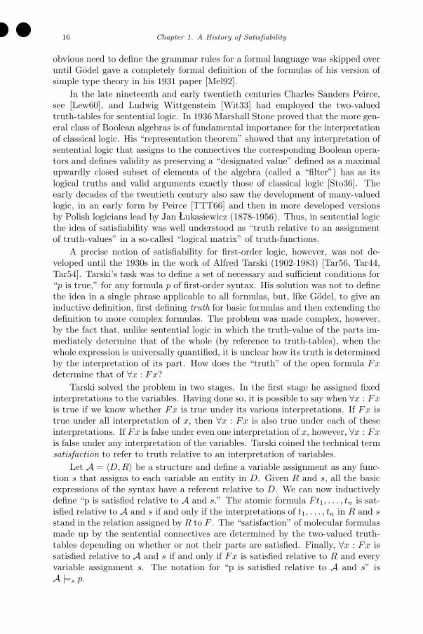
A precise notion of satisfiability for first-order logic, however, was not de-veloped until the 1930s in the work of Alfred Tarski (1902-1983) [Tar56, Tar44,Tar54]. Tarski’s task was to define a set of necessary and sufficient conditions for“p is true,” for any formula p of first-order syntax. His solution was not to definethe idea in a single phrase applicable to all formulas, but, like Godel, to give aninductive definition, first defining truth for basic formulas and then extending thedefinition to more complex formulas. The problem was made complex, however,by the fact that, unlike sentential logic in which the truth-value of the parts im-mediately determine that of the whole (by reference to truth-tables), when thewhole expression is universally quantified, it is unclear how its truth is determinedby the interpretation of its part. How does the “truth” of the open formula Fx

determine that of ∀x : Fx?

Tarski solved the problem in two stages. In the first stage he assigned fixedinterpretations to the variables. Having done so, it is possible to say when ∀x : Fx

is true if we know whether Fx is true under its various interpretations. If Fx istrue under all interpretation of x, then ∀x : Fx is also true under each of theseinterpretations. If Fx is false under even one interpretation of x, however, ∀x : Fx

is false under any interpretation of the variables. Tarski coined the technical termsatisfaction to refer to truth relative to an interpretation of variables.

Let A = 〈D,R〉 be a structure and define a variable assignment as any func-tion s that assigns to each variable an entity in D. Given R and s, all the basicexpressions of the syntax have a referent relative to D. We can now inductivelydefine “p is satisfied relative to A and s.” The atomic formula Ft1, . . . , tn is sat-isfied relative to A and s if and only if the interpretations of t1, . . . , tn in R and s

stand in the relation assigned by R to F . The “satisfaction” of molecular formulasmade up by the sentential connectives are determined by the two-valued truth-tables depending on whether or not their parts are satisfied. Finally, ∀x : Fx issatisfied relative to A and s if and only if Fx is satisfied relative to R and everyvariable assignment s. The notation for “p is satisfied relative to A and s” isA |=s p.

�

�

“p01c01˙his” — 2008/11/20 — 10:11 — page 17 — #17�

�

�

�

�

�


The second stage of Tarski’s definition is to abstract away from a variableassignment and define the simpler notion “p is true relative to A.” His idea atthis stage is to interpret an open formula Fx as true in this general sense if itis “always true” in the sense of being satisfied under every interpretation of itsvariables. That is, he adopts the simple formula: p is true relative to A if andonly if, for all variable assignments s, p is satisfied relative to A and s. In formalnotation, A |= p if and only if, for all s, A |=s p.

Logicians have adopted the common practice of using the term “satisfied in astructure” to mean what Tarski called “true in a structure.” Thus, it is commonto say that p is satisfiable if there is some structure A such that p is true in A,and that a set of formulas X is satisfiable if and only if there is some structureA such that for all formulas p in X, p is true (satisfied) in A.

1.13. Completeness of first-order logic

First-order logic has sufficient expressive power for the formalization of virtuallyall of mathematics. To use it requires a sufficiently powerful axiom system suchas the Zermelo-Fraenkel set theory with the axiom of choice (ZFC). It is generallyaccepted that all of classical mathematics can be formalized in ZFC.

Proofs of completeness of first-order logic under suitable axiom systems dateback at least to Godel in 1929. In this context, completeness means that all logi-cally valid formulas of first-order logic can be derived from axioms and rules of theunderlying axiom system. This is not to be confused with Godel’s incompletenesstheorem which states that there is no consistent axiom system for the larger setof truths of number theory (which includes the valid formulas of first-order logicas a proper subset) because it will fail to include at least one truth of arithmetic.

Tarski’s notion of truth in a structure introduced greater precision. It wasthen possible to give an elegant proof that first-order logic is complete underits usual axiom systems and sets of inference rules. Of particular interest is theproof due to Leon Henkin (1921-2006) that makes use of two ideas relevant tothis book: satisfiability and a structure composed of syntactic elements [Hen49](1949). Due to the relationship of validity to satisfiability, Henkin reformulatedthe difficult part of the theorem as: if a set of formulas is consistent, then it issatisfiable. He proved this by first extending a consistent set to what he calls amaximally consistent saturated set, and then showing that this set is satisfiablein a structure made up from the syntactic elements of the set. Although differingin detail, the construction of the structure is similar to that of Herbrand.

Herbrand models and Henkin’s maximally consistent saturated sets are rele-vant prototypes of the technique of constructing syntactic proxies for conventionalmodels. In complexity theory, the truth of predicates is typically determined rela-tive to a structure with a domain of entities that are programs or languages whichthemselves have semantic content that allow one to determine a corresponding,more conventional, model theoretic structure. In that sense, the program orlanguage entities can be said to be a proxy for the conventional model and thepredicates are second-order, standing for a property of sets.

�

�

“p01c01˙his” — 2008/11/20 — 10:11 — page 18 — #18�

�

�

�

�

�


1.14. Application of logic to circuits

Claude Shannon provided one of the bridges connecting the path of logic over thecenturies to its practical applications in the information and digital age. Anotherbridge is considered in the next section. Whereas the study of logic for thousandsof years was motivated by a desire to explain how humans use information andknowledge to deduce facts, particularly to assist in decision making, Shannon, asa student at MIT, saw propositional logic as an opportunity to make rigorousthe design and simplification of switching circuits. Boolean algebra, appreciatedby a relatively small group of people for decades, was ready to be applied to thefledgling field of digital computers.

In his master’s thesis [Sha40] (1940), said by Howard Gardner of HarvardUniversity to be “possibly the most important, and also the most famous, master’sthesis of the century,” Shannon applied Boolean logic to the design of minimalcircuits involving relays. Relays are simple switches that are either “closed,” inwhich case current is flowing through the switch or “open,” in which case currentis stopped. Shannon represented the state of a relay with a variable taking value1 if open and the value 0 if closed. His algebra used the operator ’+’ for “or”(addition - to express the state of relays in series), ’·’ for “and” (multiplication- to express the state of relays in parallel), and his notation for the negation ofvariable x was x

′.The rigorous synthesis of relay circuits entails expressing and simplifying

complex Boolean functions of many variables. To support both goals Shannondeveloped two series expansions for a function, analogous, in his words, to Taylor’sexpansion on differentiable functions. He started with

f(x1, x2, ..., xn) = x1 · f(1, x2, ..., xn) + x′1 · f(0, x2, ..., xn)

which we recognize as the basic splitting operation of DPLL algorithms andthe Shannon expansion which is the foundation for Binary Decision Diagrams(Section 1.20), and its dual

f(x1, x2, ..., xn) = (f(0, x2, ..., xn) + x1) · (f(1, x2, ..., xn) + x′1).

Using the above repeatedly he arrived at the familiar DNF canonical form

f(x1, x2, ..., xn) = f(0, 0, ..., 0) · x′1 · x

′2 · ... · x

′n +

f(1, 0, ..., 0) · x1 · x′2 · ... · x

′n +

f(0, 1, ..., 0) · x′1 · x2 · ... · x

′n +

...

f(1, 1, ..., 1) · x1 · x2 · ... · xn

and its familiar CNF dual. These support the expression of any relay circuitand, more generally, any combinational circuit. To simplify, he introduced thefollowing operations:

x = x + x = x + x + x = ...

x + x · y = x

�

�

“p01c01˙his” — 2008/11/20 — 10:11 — page 19 — #19�

�

�

�

�

�


x · f(x) = x · f(1)

x′· f(x) = x

′· f(0)

x · y + x′· z = x · y + x

′· z + y · z

and their duals. In the last operation the term y · z is the consenus of termsx · y and x′ · z. The dual of the last operation amounts to adding a propositionalresolvent to a CNF clause set. The first two operations are subsumption rules.

In his master’s thesis Shannon stated that one can use the above rules toachieve minimal circuit representations but did not offer a systematic way to doso. Independently, according to Brown [Bro03], Archie Blake, an all but forgottenyet influential figure in Boolean reasoning, developed the notion of consensus in hisPh.D. thesis [Bla37] of 1937. Blake used consensus to express Boolean functionsin a minimal DNF form with respect to their prime implicants (product g is animplicant of function h if g · h′ = 0 and is prime if it is minimal in literals)and subsumption. An important contribution of Blake was to show that DNFsare not minimized unless consensus is not possible. The notion of concensuswas rediscovered by Samson and Mills [SM54] (1954) and Quine [Qui55] (1955).Later, Quine [Qui59] (1959) and McCluskey [McC59] (1959) provided a systematicmethod for the minimization of DNF expressions through the notion of essential

prime implicants (necessary prime implicants) by turning the 2-level minimizationproblem into a covering problem. This was perhaps the first confrontation withcomplexity issues: although they did not know it at the time, the problem theywere trying to solve is NP-complete and the complexity of their algorithm wasO(3n/

√n), where n is the number of variables.

1.15. Resolution

Meanwhile, the advent of computers stimulated the emergence of the field ofautomated deduction. Martin Davis has written a history of this period in [Dav01]on which we base this section. Early attempts at automated deduction were aimedat proving theorems from first-order logic because, as stated in Section 1.13, itis accepted that given appropriate axioms as premises, all reasoning of classicalmathematics can be expressed in first-order logic. Propositional satisfiabilitytesting was used to support that effort.

However, since the complexity of the problem and the space requirements ofa solver were not appreciated at the time, there were several notable failures. Atleast some of these determined satisfiability either by simple truth table calcu-lations or expansion into DNF and none could prove anything but the simplesttheorems. But, each contributed something to the overall effort. According toDavis [Dav01], Gilmore’s [Gil60] (1960) system served as a stimulus for othersand Prawitz [Pra60] (1960) adopted a modified form of the method of seman-tic tableaux. Also notable were the “Logic Theory Machine” of [NSS57] (1957),which used the idea of a search heuristic, and the Geometry machine of [Gel59](1959), which exploited symmetry to reduce proof size.

Things improved when Davis and Putnam proposed using CNF for satisfia-bility testing as early as 1958 in an unpublished manuscript for the NSA [DP58].

�

�

“p01c01˙his” — 2008/11/20 — 10:11 — page 20 — #20�

�

�

�

�

�


According to Davis [Dav01], that manuscript cited all the essentials of modernDPLL variants. These include:

1. The one literal rule also known as the unit-clause-rule: for each clause (l),called a unit clause, remove all clauses containing l and all literals ¬l.

2. The affirmative-negative rule also known as the pure-literal-rule: if literall is in some clause but ¬l is not, remove all clauses containing l. Literal l

is called a pure literal .3. The rule for eliminating atomic formulas: that is, replace

(v ∨ l1,1 ∨ . . . ∨ l1,k1) ∧ (¬v ∨ l2,1 ∨ . . . ∨ l2,k2

) ∧ C

with(l1,1 ∨ . . . ∨ l1,k1

∨ l2,1 ∨ . . . ∨ l2,k2) ∧ C

if literals l1,i and l2,j are not complementary for any i, j.4. The splitting rule, called in the manuscript ‘the rule of case analysis.’

Observe that rule 3. is ground resolution: the CNF expression it is applied tohaving come from a prenex form with its clauses grounded. The published versionof this manuscript is the often cited [DP60] (1960). The Davis-Putnam procedure,or DPP, reduced the size of the search space considerably by eliminating variablesfrom a given expression. This was done by repeatedly choosing a target variablev still appearing in the expression, applying all possible ground resolutions on v,then eliminating all remaining clauses still containing v or ¬v.

Loveland and Logemann attempted to implement DPP but they found thatground resolution used too much RAM, which was quite limited in those days.So they changed the way variables are eliminated by employing the splittingrule: recursively assigning values 0 and 1 to a variable and solving both resultingsubproblems [DLL62] (1962). Their algorithm is, of course, the familiar DPLL.

Robinson also experimented with DPP and, taking ideas from both DPP

and Prawitz, he generalized ground resolution so that instead of clauses havingto be grounded to use resolution, resolution was lifted directly to the Skolemform [Rob63, Rob65] (1963,1965). This is, of course, a landmark result in me-chanically proving first-order logic sentences.

Resolution was extended by Tseitin in [Tse68] (1968) who showed that, forany pair of variables a, b in a given CNF expression φ, the following expressionmay be appended to φ:

(z ∨ a) ∧ (z ∨ b) ∧ (¬z ∨ ¬a ∨ ¬b)

where z is a variable not in φ. The meaning of this expression is: either a andb both have value 1 or at least one of a or b has value 0. It may be writtenz ⇔ ¬a ∨ ¬b. It is safe to append such an expression because its three clausescan always be forced to value 1 by setting free variable z to the value of ¬a∨¬b.More generally, any expression of the form

z ⇔ f(a, b, ...)

may be appended, where f is some arbitrary Boolean function and z is a new, freevariable. Judicious use of such extensions can result in polynomial size refuta-tions for problems that have no polynomial size refutations without extension. A

�

�

“p01c01˙his” — 2008/11/20 — 10:11 — page 21 — #21�

�

�

�

�

�


notable example is the pigeon hole formulas. Tseitin also showed that by addingvariables not in φ, one can obtain, in linear time, a satisfiability-preserving trans-lation from any propositional expression to CNF with at most a constant factorblowup in expression size.

After this point the term satisfiability was used primarily to describe the prob-lem of finding a model for a Boolean expression. The complexity of Satisfiabilitybecame the major issue due to potential practical applications for Satisfiability.Consequently, work branched in many directions. The following sections describemost of the important branches.

1.16. The complexity of resolution

by Alasdair Urquhart

Perhaps the theoretically deepest branch is the study of the complexity of resolu-tion. As seen in previous sections, the question of decidability dominated researchin logic until it became important to implement proof systems on a computer.Then it became clear empirically and theoretically through the amazing result ofCook [Coo71] (1971) that decidable problems could still be effectively unsolvabledue to space and time limitations of available machinery. Thus, many researchersturned their attention to the complexity issues associated with implementing var-ious logic systems. The most important of these, the most relevant to the readersof this chapter, and the subject of this section is the study of resolution refuta-tions of contradictory sets of CNF clauses (in this section clause will mean CNFclause).

Rephrasing the “rule for eliminating atomic formulas” from the previous sec-tion: if A ∨ l and B ∨ ¬l are clauses, then the clause A ∨ B may be inferred bythe resolution rule, resolving on the literal l. A resolution refutation of a set ofclauses Σ is a proof of the empty clause from Σ by repeated applications of theresolution rule.

Refutations can be represented as trees or as sequences of clauses; the worstcase complexity differs considerably depending on the representation. We shalldistinguish between the two by describing the first system as “tree resolution,”the second simply as “resolution.”

Lower bounds on the size of resolution refutations provide lower bounds onthe running time of algorithms for the Satisfiability problem. For example, con-sider the familiar DPLL algorithm that is the basis of many of the most successfulalgorithms for Satisfiability. If a program based on the splitting rule terminateswith the output “The set of clauses Σ is unsatisfiable,” then a trace of the pro-gram’s execution can be given in the form of a binary tree, where each of thenodes in the tree is labeled with an assignment to the variables in Σ. The root ofthe tree is labeled with the empty assignment, and if a node other than a leaf islabeled with an assignment φ, then its children are labeled with the assignmentsφ[v := 0] and φ[v := 1] that extend φ to a new variable v; the assignments labelingthe leaves all falsify a clause in Σ. Let us call such a structure a “semantic tree,”an idea introduced by Robinson [Rob68] and Kowalski and Hayes [KH69].

A semantic tree for a set of clauses Σ can be converted into a tree resolutionrefutation of Σ by labeling the leaves with clauses falsified by the assignment at

�

�

“p01c01˙his” — 2008/11/20 — 10:11 — page 22 — #22�

�

�

�

�

�


the leaves, and then performing resolution steps corresponding to the splittingmoves (some pruning may be necessary in the case that a literal is missing fromone of the premisses). It follows that a lower bound on the size of tree resolutionrefutations for a set of clauses provides a lower bound on the time required fora DPLL-style algorithm to certify unsatisfiability. This lower bound applies nomatter what strategies are employed for the order of variable elimination.

The first results on the complexity of resolution were proved by GrighoriTseitin in 1968 [Tse68]. In a remarkable pioneering paper, Tseitin showed thatfor all n > 0, there are contradictory sets of clauses Σn , containing O(n2) clauseswith at most four literals in each clauses, so that the smallest tree resolutionrefutation of Σn has 2Ω(n) leaves. Tseitin’s examples are based on graphs. If weassign the values 0 and 1 to the edges of a finite graph G, we can define a vertexv in the graph to be odd if there are an odd number of vertices attached to v withthe value 1. Then Tseitin’s clauses Σ(G) can be interpreted as asserting thatthere is a way of assigning values to the edges so that there are an odd number ofodd vertices. The set of clauses Σn mentioned above is Σ(Gn), where Gn is then× n square grid.

Tseitin also proved some lower bounds for resolution but only under the re-striction that the refutation is regular. A resolution proof contains an irregularity

if there is a sequence of clauses C1, . . . , Ck in it, so that Ci+1 is the conclusion of aresolution inference of which Ci is one of the premisses, and there is a variable v sothat C1 and Ck both contain v, but v does not occur in some intermediate clauseCj , 1 < j < k. In other words, an irregularity occurs if a variable is removed byresolution, but is later introduced again in a clause depending on the conclusionof the earlier step. A proof is regular if it contains no irregularity. Tseitin showedthat the lower bound for Σn also applies to regular resolution. In addition, heshowed that there is a sequence of clauses Πn so that there is a superpolynomialspeedup of regular resolution over tree resolution (that is to say, the size of thesmallest tree resolution refutation of Πn is not bounded by any fixed power of thesize of the smallest regular refutation of Πn).

Tseitin’s lower bounds for the graph-based formulas were improved by ZviGalil [Gal77], who proved a truly exponential lower bound for regular resolutionrefutations of sets of clauses based on expander graphs En of bounded degree. Theset of clauses Σ(En) has size O(n), but the smallest regular resolution refutationof Σ(En) contains 2Ω(n) clauses.

The most important breakthrough in the complexity of resolution was madeby Armin Haken [Hak85], who proved exponential lower bounds for the pigeonholeclauses PHCn. These clauses assert that there is an injective mapping from theset {1, . . . , n + 1} into the set {1, . . . , n}. They contain n + 1 clauses containingn literals asserting that every element in the first set is mapped to some elementof the second, and O(n3) two-literal clauses asserting that no two elements aremapped to the same element of {1, . . . , n}. Haken showed that any resolutionrefutation of PHCn contains 2Ω(n) clauses.

Subsequently, Urquhart [Urq87] adapted Haken’s argument to prove a trulyexponential lower bound for clauses based on expander graphs very similar tothose used earlier by Galil. The technique used in Urquhart’s lower bounds wereemployed by Chvatal and Szemeredi [CS88] to prove an exponential lower bound

�

�

“p01c01˙his” — 2008/11/20 — 10:11 — page 23 — #23�

�

�

�

�

�


on random sets of clauses. The model of random clause sets is that of the constantwidth distribution discussed below in Section 1.18. Their main result is as follows:if c, k are positive integers with k ≥ 3 and c2−k ≥ 0.7, then there is an ε > 0, sothat with probability tending to one as n tends to infinity, the random family ofcn clauses of size k over n variables is unsatisfiable and its resolution complexityis at least (1 + ε)n.

The lower bound arguments used by Tseitin, Galil, Haken and Urquhart havea notable common feature. They all prove lower bounds on size by proving lowerbounds on width – the width of a clause is the number of literals it contains,while the width of a set of clauses is the width of the widest clause in it. If Σ is acontradictory set of clauses, let us write w(Σ) for the width of Σ, and w(Σ � 0)for the minimum width of a refutation of Σ.

The lower bound techniques used in earlier work on the complexity of res-olution were generalized and unified in a striking result due to Ben-Sasson andWigderson [BSW01]. If Σ is a contradictory set of clauses, containing the vari-ables V , let us write S(Σ) for the minimum size of a resolution refutation of Σ.Then the main result of [BSW01] is the following lower bound:

S(Σ) = exp

(Ω

((w(Σ � 0)− w(Σ))2

|V |

)).

This lower bound easily yields the lower bounds of Urquhart [Urq87], as wellas that of Chvatal and Szemeredi [CS88] via a width lower bound on resolutionrefutations.

Tseitin was the first to show a separation between tree resolution and generalresolution, as mentioned above. The separation he proved is fairly weak, thoughsuperpolynomial. Ben-Sasson, Impagliazzo and Wigderson [BSIW04] improvedthis to a truly exponential separation between the two proof systems, using con-tradictory formulas based on pebbling problems in directed acyclic graphs.

These results emphasize the inefficiency of tree resolution, as opposed togeneral resolution. A tree resolution may contain a lot of redundancy, in thesense that the same clause may have to be proved multiple times. The same kindof inefficiency is also reflected in SAT solvers based on the DPLL framework,since information accumulated along certain branches is immediately discarded.This observation has led some researchers to propose improved versions of theDPLL algorithm, in which such information is stored in the form of clauses.These algorithms, which go under the name “clause learning,” lead to dramaticspeedups in some cases – the reader is referred to the paper of Beame, Kautz andSabharwal [BKS03] for the basic references and some theoretical results on themethod.

1.17. Refinement of Resolution-Based SAT Solvers

Most of the current interest in Satisfisfiability formulations and methods is dueto refinements to the basic DPLL framework that have resulted in speed-ups ofmany orders of magnitude that have turned many problems that were consideredintractable in the 1980s into trivially solved problems now. These refinements

�

�

“p01c01˙his” — 2008/11/20 — 10:11 — page 24 — #24�

�

�

�

�

�


include improvements to variable choice heuristics, early pruning of the searchspace, and replacement of a tree-like search space with a DAG-like search space.

DPLL (1962) was originally designed with two important choice heuristics:the pure-literal rule and the unit-clause rule (Both described on Page 20). But,variable choices in case no unit clauses or pure literals exist were undefined.Thus, extensions of both heuristics were proposed and analyzed in the 1980sthrough the early 2000s. For example, the unit-clause rule was generalized tothe shortest-clause rule: choose a variable from an existing clause containing thefewest unset literals [CF90, CR92] (1990, described on Page 37) and the pure-literal rule was extended to linear autarkies [vM00] (2000, described on Page 29).Other notable analyzed heuristics include the majority rule: choose a variablewith the maximum difference between the number of its positive and negativeliterals [CF86] (1986, see also Page 37), probe-order backtracking [PH97] (1997,see also Page 36), and a greedy heuristic [HS03, KKL04] (2003, described onPage 38). The above heuristics represent parts of many heuristics that haveactually been implemented in SAT solvers; they were studied primarily becausetheir performance could be analyzed probabilistically.

Early heuristics designed to empirically speed up SAT solvers were based onthe idea that eliminating small clauses first tends to reveal inferences sooner. Pos-sibly the earliest well-known heuristic built on this approach is due to Jeroslowand Wang [JW90] (1990): they choose a value for a variable that comes close tomaximizing the chance of satisfying the remaining clauses, assuming the remain-ing clauses are statistically independent in the sense described on Page 37. Theyassign weights w(Si,j) for each variable vj and each value i ∈ {0, 1} where, for asubset of clauses S, Si,j is the clauses of S less those clauses satisfied and thoseliterals falsified by assigning value i to vj and w(Si,j) =

∑C∈Si,j

2−|C| (|C| is the

width of clause C). The Jeroslow-Wang heuristic was intended to work betteron satisfiable formulas but Bohm [BKB92] (1992) and Freeman [Fre95] (1995)came up with heuristics that work better on unsatisfiable formulas: they chooseto eliminate a variable that in some sense maximally causes an estimate of bothsides of the resulting search space to be roughly of equal size. This can be done,for example, by assigning variable weights that are the product of positive andnegative literal weights as above and choosing the variable of maximum weight.Later, it was observed that the activity of variable assignment was an importantfactor in search space size. This led to the DLIS heuristic of GRASP [MSS96]and eventually to the VSIDS heuristic of Chaff [MMZ+01]. Most recent DPLLbased SAT solvers use variations of the VSIDS branching heuristic.

Another important refinement to SAT solvers is the early generation of in-ferences during search. This has largely taken the appearance of lookahead tech-niques. It was Stalmarck [SS98] who demonstrated the effectiveness of lookaheadin Prover (1992): the particular type of lookahead used there is best describedas breadth-first. This scheme is limited by the fact that search space width canbe quite large so the lookahead must be restricted to a small number of levels,usually 2. Nevertheless, Prover was regarded to be a major advance at the time.Later, Chaff used depth-first lookahead (this form is generally called restarts)to greater effectiveness [MMZ+01]. Depth-first lookahead also solves a problemthat comes up when saving non-unit inferences (see below): such inferences may

�

�

“p01c01˙his” — 2008/11/20 — 10:11 — page 25 — #25�

�

�

�

�

�


be saved in a cache which may possibly overflow at some point. In the case ofdepth-first lookahead, the inferences may be applied and search restarted with acleared cache.

Extremely important to SAT solver efficiency are mechanisms that reducethe size of the search space: that is, discover early that branch of the searchspace does not have to be explored. A conflict analysis at a falsified node of thesearch space will reveal the subset Vs of variables involved in that node becomingfalse. Thus, the search path from root to that falsified node can be collapsedto include only the variables in Vs, effectively pruning many branch points fromthe search space. This has been called non-chronological backtracking [MSS96](1996) and is seen in all of the most efficient DPLL based SAT solvers. Theresult of conflict analysis can also be saved as a non-unit inference in the formof a clause. If later in the search a subset of variables are set to match a savedinference, backtracking can immediately be applied to avoid repeating a searchthat previously ended with no solution. This idea, known as clause learning, isan essential part of all modern DPLL based SAT solvers: its power comes fromturning what would be a tree-like search space into a DAG-like search space.This has gone a long way toward mitigating the early advantage of BDDs (seeSection 1.20) over search: BDD structures are non-repetitive. In practice, clauselearning is often implemented jointly with the opportunistic deletion of the lessused learnt clauses, thus reducing the over-usage of physical memory by SATsolvers. Nevertheless, several of the most efficient DPLL based SAT solvers optfor not deleting any of the learnt clauses, and so the need for deleting less usedlearnt clauses is still not a completely solved issue.

Finally, the development of clever data structures have been crucial to SATsolver success. The most important of these is the structure that supports thenotion of the watched literal [MMZ+01].

1.18. Upper bounds

by Ewald Speckenmeyer

Deciding satisfiability of a CNF formula φ with n Boolean variables can be per-formed in time O(2n|φ|) by enumerating all assignments of the variables. Thenumber m of clauses as well as the number l of literals of φ are further parame-ters for bounding the runtime of decision algorithms for SAT. Note that l is equalto length(φ) and this is the usual parameter for the analysis of algorithms. Mosteffort in designing and analyzing algorithms for SAT solving, however, are basedon the number n of variables of φ.

A first non-trivial upper bound of O(αnk · |φ|), where αn

k is bounding theFibonacci-like recursion

T (1) = T (2) = . . . = T (k − 1) = 1 and

T (n) = T (n− 1) + T (n− 2) + . . . + T (n− k + 1), for n ≥ k,

for solving k-SAT, k ≥ 3, was shown in [MS79, MS85]. For example, α3 ≥ 1.681,α4 ≥ 1.8393, and α5 ≥ 1.9276.

�

�

“p01c01˙his” — 2008/11/20 — 10:11 — page 26 — #26�

�

�

�

�

�


The algorithm supplying the bound looks for a shortest clause c from thecurrent formula. If c has k− 1 or less literals, e.g. c = (x1 ∨ . . .∨ xk−1) then φ issplit into k − 1 subformulas according to the k − 1 subassignments

1) x1 = 1;2) x1 = 0, x2 = 1;

. . .

k-1) x1 = x2 = . . . = xk−2 = 0, xk−1 = 1.

If all clauses c of φ have length k, then φ is split into k subformulas as described,and each subformula either contains a clause of length at most k−1 or one of theresulting subformulas only contains clauses of length k. In the former case, theabove mentioned bound holds. In the latter case, the corresponding subassign-ment is autark, that is, all clauses containing these variables are satisfied by thissubassignment, so φ can be evaluated according to this autark subassignmentthereby yielding the indicated upper bound.

For the case k = 3, the bound was later improved to α3 = 1.497 by a so-phisticated case analysis (see [Sch96]). Currently, from [DGH+02], the best de-terministic algorithms for solving k-SAT have a run time of

O

((2−

2

k + 1)n

).

For example, the bounds are O(1.5n), O(1.6n), O(1.666...n) for 3, 4, and 5literal clause formulas. These bounds were obtained by the derandomization of amultistart-random-walk algorithm based on covering codes. In the case of k = 3the bound has been further improved to O(1.473n) in [BK04]. This is currentlythe best bound for deterministic 3-SAT solvers.

Two different probabilistic approaches to solving k-SAT formulas have re-sulted in better bounds and paved the way for improved deterministic bounds.The first one is the algorithm of Paturi-Pudlak-Zane [PPZ97] which is based onthe following procedure:

Determine a truth assignment of the variables of the input formula φ byiterating over all variables v of φ in a randomly chosen order: If φ containsa unit clause c = (x), where x = v or ¬v, set t(v) such that t(x) = 1. Ifneither v nor ¬v occur in a unit clause of φ, then randomly choose t(v)from {0, 1}. Evaluate φ := t(φ). Iterate this assignment procedure atmost r times or until a satisfying truth assignment t of φ is found, startingeach time with a randomly chosen order of variables for the assignmentprocedure.

After r = 2n(1− 1k) rounds a solution for a satisfiable formula is found with high

probability [PPZ97]. By adding to φ clauses originating from resolving inputclauses up to a certain length this bound can be improved. In case of k = 3,4, and 5, the basis of the exponential growth function is 1.36406, 1, 49579, and1, 56943 [PPZ98]. For k ≥ 4 this is currently the best probabilistic algorithm forsolving k-SAT.

The second approach is due to Schoning [Sch99, Sch02] and extends an idea

�

�

“p01c01˙his” — 2008/11/20 — 10:11 — page 27 — #27�

�

�

�

�

�


of Papadimitriou [Pap91]. That procedure is outlined as follows:

Repeat the following for r rounds: randomly choose an initial truth as-signment t of φ; if t does not satisfy φ, then repeat the following for threetimes the number of variables of φ or until a satisfying assignment t is en-countered: select a falsified clause c from φ and randomly choose and flipa literal x of c.

If the algorithm continues, round after round, without finding a satisfying assign-ment nothing definite can be said about the satisfiability of φ. However, in thiscase the higher the number of rounds r, the lower the probability that φ is satis-fiable. To guarantee an error probability of e−λ, the number of rounds should beat least O(λ(2k−1

k )n). For k = 3, 4, and 5 the basis of the exponential growth is1.3334, 1.5, and 1.6.

The case of k = 3 has since been improved to O(1.324n) by Iwama andTamaki [IT03]. For CNF formulas of unrestricted clause length the best time

bound for a deterministic solution algorithm is O(2n(1− 1log(2m)

)), where n is thenumber of variables and m the number of clauses. This result, by Dantsin andWolpert [DW04], is obtained from a derandomization of a randomized algorithmby Schuler [Sch05], of the same time complexity. Dantsin and Wolpert recently im-

proved this bound for randomized algorithms to O

(2

n(1− 1ln( m

n)+O ln(ln(m)

))

[DW05].

1.19. Classes of easy expressions

An entire book could be written about the multitude of classes of the Satisfiabilityproblem that can be solved in polynomial time, so only some of the classical resultswill be mentioned here. It is often not enough that a class of problems is solvedin polynomial time - an instance may have to be recognized as a member of thatclass before applying an efficient algorithm. Perhaps surprisingly, for some classesthe recognition step is unnecessary and for some it is necessary but not known tobe tractable.

The reader may have the impression that the number of polynomial timesolvable classes is quite small due to the famous dichotomy theorm of Schae-fer [Sch73]. But this is not the case. Schaefer proposed a scheme for definingclasses of propositional expressions with a generalized notion of “clause.” Heproved that every class definable within his scheme was either NP-complete orpolynomial-time solvable, and he gave criteria to determine which. But not allclasses can be defined within his scheme. The Horn and XOR classes can be butwe will describe several others including q-Horn, extended Horn, CC-balancedand SLUR that cannot be so defined. The reason is that Schaefer’s scheme islimited to classes that can be recognized in log space.

All clauses of a 2-SAT expression contain at most two literals. A two literalclause describes two inferences. For example, inferences for the clause (x∨y) are:1) if x is 0 then y is 1; and 2) if y is 0 then x is 1. For a given 2-SAT expressionan implication graph may be constructed where directed edges between pairsof literals represent all the inferences of the expression. A cycle in the inference

�

�

“p01c01˙his” — 2008/11/20 — 10:11 — page 28 — #28�

�

�

�

�

�


graph that includes a pair of complementary literals is proof that no model exists.Otherwise a model may be determined easily with a depth-first search of thegraph, which amounts to applying unit propagation. A full algorithm is givenin [EIS76] (1976). A linear time algorithm is given in [APT79] (1979).

All clauses of an expression said to be Horn have at most one positive literal.This class is important because of its close association with Logic Programming:for example, the clause (¬v1∨¬v2∨v) expresses the rule v1∧v2 → v or v1 → v2 →

v. However, the notion of causality is generally lost when translating from rules toHorn expressions. An extremely important property of Horn expressions is thatevery satisfiable one has a unique minimum model with respect to 1 (the uniqueminimum model is the intersection of all models of the expression). Findinga model is a matter of applying unit propagation on positive literals until allpositive literals are eliminated, then assigning all remaining literals the value 0 (ifsatisfiable, a unique minimum model is the result). It took a few iterations in theliterature to get this universally understood and the following are the importantcitations relating to this:[IM82] (1982), [DG84] (1984), [Scu90] (1990).

A given expression may be renameable Horn, meaning a change in the polarityof some variables results in an equivalent Horn expression. Renameable Hornexpressions were shown to be recognized and solved in linear time by [Lew78](1978) and [Asp80] (1980).

A number of polynomially solvable relaxations of Linear Programming prob-lems were shown to be equivalent to classes of Satisfiability; this work, quitenaturally, originated from the Operations Research community. RepresentingCNF expressions as (0,±1) matrices where columns are indexed on variables androws indexed on clauses, Satisfiability may be cast as an Integer Programmingproblem. If the matrix has a particular structure the Integer Program can berelaxed to a Linear Program, solved, and the non-integer values of the solutionrounded to 0 or 1. Notable classes based on particular matrix structures are theextended Horn expressions and what we call the CC-balanced expressions.

The class of extended Horn expressions was introduced by Chandru andHooker [CH91] (1991). Their algorithm is due to a theorem of Chandrasekaran[Cha84] (1984). Essentially, a model for a satisfiable expression may be foundby applying unit propagation, setting values of unassigned variables to 1/2 whenno unit clauses remain, and rounding the result by a matrix multiplication. Thisalgorithm cannot, however, be reliably applied unless it is known that a givenexpression is extended Horn and, unfortunately, the problem of recognizing anexpression as extended Horn is not known to be solved in polynomial time.

The class of CC-balanced expressions has been studied by several researchers(see [CCK+94] (1994) for a detailed account of balanced matrices and a descrip-tion of CC-balanced formulas). The motivation for this class is the question, forSatisfiability, when do Linear Programming relaxations have integer solutions?The satisfiability of a CNF expression can be determined in linear time if it isknown to be CC-balanced and recognizing that a formula is CC-balanced takeslinear time.

Horn, Renameable Horn, Extended Horn, CC-balanced expressions, and otherclasses including that of [SW95] (1991) turn out to be subsumed by a larger, effi-ciently solved class called SLUR for Single Lookahead Unit Resolution [SAFS95]

�

�

“p01c01˙his” — 2008/11/20 — 10:11 — page 29 — #29�

�

�

�

�

�


(1995). The SLUR class is peculiar in that it is defined based on an algorithmrather than on properties of expressions. The SLUR algorithm recursively selectsvariables sequentially and arbitrarily, and considers a one-level lookahead, underunit propagation in both directions, choosing only one, if possible. If a modelis found, the algorithm is successful, otherwise it “gives up.” An expression isSLUR if, for all possible sequences of variable selections, the SLUR algorithmdoes not give up. Observe that due to the definition of this class, the question ofclass recognition is avoided. In fact, SLUR provides a way to avoid preprocessingor recognition testing for several polynomial time solvable classes of SAT whenusing a reasonable variant of the DPLL algorithm.

The worst case time complexity of the SLUR algorithm would appear tobe quadratic. However, a simple modification brings the complexity down tolinear: run both calls of unit propagation simultaneously, alternating executionof their repeat blocks. When one terminates without an empty clause in its outputformula, abandon the other call.

The q-Horn class also originated in the Operations Research community[BCH90, BHS94] (1990) and for several years was thought to be what was describedas the largest, succinctly expressed class of polynomial time solvable expressions.This claim was due to a measure on an underlying (0,±1) matrix representationof clauses called the satisfiability index [BCHS94] (1994). The q-Horn class wasalso studied as a special case of the maximum monotone decomposition of matri-ces [Tru94] (1994). We find it easier to describe the efficient solution of q-Hornexpressions by following [Tru98] (1998). Using the (0,±1) matrix representation,an expression is q-Horn if columns can be multiplied by -1, and permuted, androws can be permuted with the result that the matrix has four quadrants asfollows: northeast - all 0s; northwest - a Horn expression; southeast - a 2-SAT ex-pression; southwest - no +1s. A model may be found in linear time, if one exists,by finding a model for the northwest quadrant Horn expression, cancelling rowsin the southern quadrants whose clauses are satisfied by that model, and findinga model for the southeast quadrant 2-SAT expression. It was shown in [BCHS94](1994) that a CNF expression is q-Horn if and only if its satisfiability index is nogreater than 1 and the class of all expressions with a satisfiability index greaterthan 1+1/n

ε, for any fixed ε < 1, is NP-complete. The SLUR and q-Horn classesare incomparable [FVG03] (2003).

The class of linear autarkies, developed by Kullmann [Kul00] (2000), wasshown by van Maaren [vM00] (2000) to include the class of q-Horn formulas. Itwas also shown to be incomparable with the SLUR class. An autarky for a CNFformula φ is a partial assignment that satisfies all those clauses of φ affected byit: for example, a pure literal is an autarky. Therefore, a subformula obtained byapplying an autarky to φ is satisfiable if and only if φ is. A formula with (0,±1)matrix representation A has a linear autarky x ∈ Qn, x = 0, if Ax ≥ 0. In [Kul00]it was shown that a linear autarky can be found in polynomial time. There existsa simple, efficient decomposition that results in a partial, autark assignment.Applying this decomposition repeatedly results in a unique, linear-autarky-freeformula. If the decomposition is repeatedly applied to a renameable Horn formulawithout unit clauses what is left is empty and if it is applied repeatedly to a 2-SATformula, the formula is unsatisfiable if what is left is not empty and satisfiable

�

�

“p01c01˙his” — 2008/11/20 — 10:11 — page 30 — #30�

�

�

�

�

�


otherwise.The class of matched expressions was analyzed to provide a benchmark for

testing the claim made for the q-Horn class. This is a class first describedin [Tov84] (1984) but not extensively studied, probably because it seems tobe a rather useless and small class of formulas. Establish a bipartite graphGφ = (V1, V2, E) for an expression φ where V1 vertices represent clauses, V2

vertices represent variables, and edge 〈c, v〉 ∈ E if and only if clause c containsv or its complement. If there is a total matching in Gφ, then φ is said to bematched. Clearly, matched expression are always satisfiable and are triviallysolved. The matched class is incomparable with the q-Horn and SLUR classes.However, as is shown in Section 1.22, with respect to frequency of occurrence onrandom expressions, matched expressions are far more common than both thoseclasses together [FVG03] (2003).

The worst case complexity of nested satisfiability, a class inspired by Lichten-stein’s theorem of planar satisfiability [Lic82] (1982), has been studied in [Knu90](1990). Index all variables in an expression consecutively from 1 to n and let pos-itive and negative literals take the index of their respective variables. A clause ci

is said to straddle another clause cj if the index of a literal of cj is strictly betweentwo indices of literals of ci. Two clauses are said to overlap if they straddle eachother. A formula is said to be nested if no two clauses overlap. For example, thefollowing formula is nested

(v6 ∨ ¬v7 ∨ v8) ∧ (v2 ∨ v4) ∧ (¬v6 ∨ ¬v9) ∧ (v1 ∨ ¬v5 ∨ v10).

The class of nested formulas is quite limited in size for at least the reason that anested expression can contain no more than 2m + n literals. Thus, no expressionconsisting of k-literal clauses is a nested formula unless m/n < 1/(k−2). The classof nested expressions is incomparable with both the SLUR and q-Horn classes.However, by the measure of Section 1.22 (also in [FVG03] (2003)) a randomexpression is far more likely to be matched, q-Horn, or even SLUR than nested.The algorithm for nested expressions is notable for being quite different thanthose mentioned above: instead of relying on unit propagation, it uses dynamicprogramming to find a model in linear time. The question of whether the variableindices of a given formula can, in linear time, be permuted to make the formulanested appears to be open. An extension to nested satisfiability, also solvable inlinear time, has been proposed in [HJP93] (1993).

None of the classes above covers a significant proportion of unsatisfiable ex-pressions. Nevertheless, several classes of unsatisfiable expressions have beenidentified. It is interesting that most known polynomial time solvable classeswith clauses containing three or more literals either are strongly biased towardsatisfiable expressions or strongly biased toward unsatisfiable expressions.

An expression is said to be minimally unsatisfiable if it is unsatisfiable andremoving any clause results in a satisfiable expression. A minimally unsatisfiableexpression with n variables must have at least n+1 clauses [AL86] (1986). Everyvariable of a minimally unsatisfiable expression occurs positively and negatively inthe expression. The class of minimally unsatisfiable formulas is solved in n

O(k) ifthe number of clauses exceeds the number of variables by a fixed positive constantk [KB99] (1999) and [KB00] (2000). Szeider improved this to O(2k)n4 [Sze03]

�

�

“p01c01˙his” — 2008/11/20 — 10:11 — page 31 — #31�

�

�

�

�

�


(2003). Kullmann has generalized this class in [Kul03] (2003) and continues tofind larger versions. Some SAT solvers look for minimally unsatisfiable sets ofclauses to reduce search space size.

A CNF expression is said to be k-BRLR if all resolvents derived from it havea number of literals bounded by k or if the null clause is deriveable from resolventshaving at most k literals. Obviously, this class is solved in time bounded by 2k

(nk

).

Finally, we mention that semidefinite programming which is discussed atlength in Section 1.25 is biased toward verifying unsatisfiability and this accountsfor the success of this approach.

1.20. Binary Decision Diagrams

Binary Decision Diagrams (BDDs) were considered for a while to be the best wayto handle some problems that are rooted in real applications, particularly relatedto circuit design, testing, and verification. They are still quite useful in variousroles [DK03, FKS+04, HD04, JS05, MM02, PV05, CGGT97] and in some waysare complementary to search [US94, GZ03].

A BDD may be regarded as a DAG representation of the truth table of aBoolean function. In a BDD non-leaf vertices are labeled as variables, there aretwo out-directed edges for each non-leaf vertex, each labeled with value 0 or 1,and two leaves, labeled 1 and 0. There is a single root and any path from root toa “1” (“0”) leaf indicates an assignment of values to the variables which causesthe represented function to have value 1 (0). A BDD may also be viewed asrepresenting a search space in which paths to the 1 leaf represent models.

The attraction to BDDs is due in part to the fact that no subproblem isrepresented more than once in a collection of BDDs - this is in contrast to the tree-like search spaces of DPLL implementations of the 1980s. In addition, efficientimplementations exist for BDD operations such as existential quantification, “or,”“and,” and others. The down side is: 1) each path from the root of a BDDmust obey the same variable ordering, so BDDs are not necessarily a minimalrepresentation for a function; and 2) repeatedly conjoining pairs of BDDs maycreate outragiously large intermediate BDDs even though the final BDD is small.By the late 1990s, DPLL advances such as conflict resolution, clausal learning,backjumping, restarts, and more gave rise to DAG search spaces with dynamicvariable ordering. The result was improved performance for search over BDDs insome cases.

BDDs were introduced in [Lee59] (1959) as a data structure based on theShannon expansion (see Section 1.14). They were publicized in [Bou76] (1976)and [Ake78] (1978). But BDDs became most useful with the introduction of re-duced order BDDs by Bryant [Bry86, Bry92] (1986,1992) and their implementa-tion [BRB90] (1990) which supports subproblem sharing over collections of BDDsand the efficient manipulation of those BDDs.

A number of operations on BDDs have been proposed over the years to assistin the efficiency of combining BDDs. One of the most important and basic op-erations is existential quantification which arises directly from Shannon’sexpansion of Section 1.14: namely, replace f with f |v=0 ∨ f |v=1. This operationcan be used to eliminate a variable at the expense of first conjoining all BDDs

�

�

“p01c01˙his” — 2008/11/20 — 10:11 — page 32 — #32�

�

�

�

�

�


containing it. It is not clear when existential quantification was first used but itwas probably known very early. An important problem in managing BDD size ishow to simplify a function f (implemented as a BDD), given a constaint c (imple-mented as a BDD): that is, replace f with a function f ′ that is equal to f on thedomain defined by c. The operation of restrict [CBM90] (1990) does this bypruning paths from the BDD of f that are ‘false’ in the BDD of c. A more com-plex operation with restrict-like properties but admiting removal of a BDD froma collection of BDDs at the expense of increasing the size of some of the remain-ing BDDs is the constrain or generalized cofactor operation [CM90] (1990).Constraining f to c results in a function h with the property that h(x) = f(μ(x))where μ(x) is the closest point to x in c where distance between binary vectorsx, y ∈ {0, 1}n is measured by d(x, y) =

∑1≤i≤n 2n−i · ((xi + yi) mod 2) under

a BDD variable ordering which matches the index order. Additional minimiza-tion operations, based on restrict, that do not increase BDD size are proposedin [HBBM97] (1997).

BDDs were designed primarily for the efficient representation of switching cir-cuits and their manipulation, but a number of variations on BDDs have appearedover the years to target related classes of problems. BDDs of various kinds havebeen used successfully to represent relations and formulas to support symbolicmodel checking [BCM+92, McM93] (1992), although more recently, it has beenfound that SAT solvers for Bounded Model Checking [BCCZ99] (1999) can some-times achieve even better results. The ZDD, for Zero-suppressed BDD, introducedin 1993 [Min93], differs from the BDD in that a vertex is removed if its 1 edgepoints to the 0 leaf. This helps improve efficiency when handling sparse sets andrepresenting covers. Thus, the ZDD has been used successfully on problems inlogic synthesis such as representing an irredundant DNF of an incompletely spec-ified Boolean function [CMFT93] (1993), finding all essential prime implicants inDNF minimization [Cou94] (1994), factorization [Min96] (1996), and decomposi-tion [JM01] (2001). The BMD, for Binary Moment Diagram, is a generalizationof the BDD for handling numbers and numeric computations, particularly multi-plication [BC95] (1995). The ADD, for Algebraic Decision Diagram (also knownas Multi-Terminal Decision Diagram), allows more than two leaves (possibly real-valued) and is useful for mapping Boolean functions to sets [BFG+93] (1993) asmight be needed to model the delay of MOS circuits, for example [MB01] (2001).The XDD has been used to efficiently represent equations involving the xor op-eration. The essential idea is that vertex x with 1 edge to vertex a and 0 edge tovertex b represents the equation (x ∧ a) ⊕ b = 1. Many other varieties of BDDhave been proposed but there is not enough space to mention them all.

1.21. Probabilistic analysis: SAT algorithms

Probabilistic and average-case analysis of algorithms can give useful insight intothe question of what SAT algorithms might be effective and why. Under certaincircumstances, one or more structural properties shared by each of a collectionof formulas may be exploited to solve such formulas efficiently; or structuralproperties might force a class of algorithms to require superpolynomial time.Such properties may be identified and then, using probabilistic analysis, one may

�

�

“p01c01˙his” — 2008/11/20 — 10:11 — page 33 — #33�

�

�

�

�

�


argue that these properties are so common that the performance of an algorithmor class of algorithms can be predicted for most of a family of formulas. The firstprobabilistic results for SAT had this aim.

Probabilistic results of this sort depend on an underlying input distribution.Although many have been proposed, well-developed histories exist for just two,plus a few variants, which are defined over CNF inputs. All the results of thissection are based on these two. In what follows, the width of a clause is thenumber of literals it contains. The distributions we discuss here are:

1. Variable width distribution: Given integers n, m, and a function p :N+ × N+ → [0, 1]. Let V = {v1, ..., vn} be a set of n Boolean vari-ables. Construct a random clause (disjunction) c by independently addingliterals to c as follows: for each variable vi, 1 ≤ i ≤ n, add literal vi withprobability p(m,n), add literal ¬vi with probability p(m,n) (therefore addneither vi nor ¬vi with probability 1−2p(m,n)). A random input consistsof m independently constructed random clauses and is referred to below asa random (n,m, p)-CNF expression. In some cases p(m,n) is independentof m and n and then we use p to represent p(m,n).

2. Constant width distribution: Given integers n, m, and k. Let V = {v1, ..., vn}

be a set of n Boolean variables. Construct a random clause (disjunction) c

by choosing, uniformly and without replacement, k variables from V andthen complementing each, independently, with probability 1/2. A ran-dom input consists of m independently constructed random clauses and isreferred to below as a random (n,m, k)-CNF expression. Such an inputis widely known as a uniform random k-SAT instance or simply randomk-SAT instance.

1.21.1. Variable width distribution

Goldberg was among the first to apply probability to the analysis of SAT algo-rithms. He investigated the frequency with which simple backtracking returns amodel quickly on random CNF formulas by providing an average-case analysis ofa variant of DPLL which does not handle pure literals or unit clauses [Gol79](1979). The result received a lot of attention when it was first presented and even10 years afterward some people still believed it was the definitive probabilisticresult on satisfiability algorithms.

Goldberg showed that, for random (n,m, p)-CNF expressions, the DPLL

variant has average complexity bounded from above by O(m−1/ log(p)n) for anyfixed 0 < p < 1. This includes the “unbiased” sample space when p = 1/3 andall expressions are equally likely. Later work [GPB82] (1982) showed the sameaverage-case complexity even if pure literals are handled as well. Very manyproblems confronting the scientific and engineering communities are unsatisfiable,but Goldberg made no mention of the frequency of occurrence of unsatisfiablerandom (n,m, p)-CNF expressions.

However, Franco and Paull [FP83] (1983) pointed out that large sets of ran-dom (n,m, p)-CNF expressions, for fixed 0 < p < 1/2, are dominated by trivialsatisfiable expressions: that is, any random assignment of values to the variablesof such a random expression is a model for that expression with high probabil-

�

�

“p01c01˙his” — 2008/11/20 — 10:11 — page 34 — #34�

�

�

�

�

�


ity. This result is refined somewhat in [Fra86b] (1986) where it is shown that arandom assignment is a model for a random (n,m, p)-CNF expression with highprobability if p > ln(m)/n and a random expression is unsatisfiable with highprobability if p < ln(m)/2n. In the latter case, a “proof” of unsatisfiability istrivially found with high probability because a random (n,m, k)-CNF expressionfor this range of p usually contains at least one empty clause, which can easilybe located, and implies unsatisfiability. The case p = c ln(m)/n, 1/2 ≤ c ≤ 1 wasconsidered in [FH89] (1988) where it was shown that a random (n,m, p)-CNFexpression is satisfiable with high probability if limn,m→∞ m1−c/n1−ε < ∞, forany 0 < ε < 1.

Although these results might be regarded as early threshold results (see Sec-tion 1.22) the main impact was to demonstrate that probabilistic analysis can behighly misleading and requires, among other things, some analysis of input distri-bution to ensure that a significant percentage of non-trivial inputs are generated.They show that random (n,m, p)-CNF expressions, satisfiable or unsatisfiable,are usually trivially solved because either they contain empty clauses (we get thesame result even if empty or unit clauses are disallowed) or they can be satisfied bya random assignment. In other words, only a small region of the parameter spaceis capable of supporting significantly many non-trivial expressions: namely, whenthe average clause width is c ln(m)/n, 1/2 ≤ c ≤ 1. These results demonstrateshortcomings in choosing random (n,m, p)-CNF expressions for analysis and, be-cause of this, such generators are no longer considered interesting by many.

Nevertheless, some interesting insights were developed by further analysisand we mention the most significant ones here. The results are shown graphicallyin Figure 1.1 which partitions the entire parameter space of the variable widthdistribution according to polynomial-average-time solvability. The vertical axis(p · n) measures average clause width and the horizontal axis (m/n) measuresdensity. Each result is presented as a line through the chart with a perpendiculararrow. Each line is a boundary for the algorithm labeling the line and the arrowindicates that the algorithm has polynomial average time performance in thatregion of the parameter space that is on the arrow side of the line (constant andeven log factors are ignored for simplicity).

Goldberg’s result is shown as the diagonal line in the upper right corner of thefigure and is labeled Goldberg: it is not even showable as a region of the param-eter space, so there is no arrow there. Iwama analyzed an algorithm which countsmodels using inclusion-exclusion [Iwa89] (1989) and has polytime-average-timecomplexity in the region above and to the right of the line labeled Counting. Arandom expression generated at a point in that region satisifes conditions, withhigh probability, under which the number of terms in the inclusion-exclusion ex-pansion is polynomial in m and n. However, every clause of the same randomexpression is a tautology (contains a literal and its complement) with high prob-ability. Therefore, this seems to be another example of a misleading result and,judging from the relation between the Counting and Goldberg regions in thefigure, lessens the significance of Goldberg’s result even more.

There have been a number of schemes proposed for limiting resolution stepsto obtain polynomial complexity. A simple example is to perform resolution onlyif the pivot variable appears once as a positive literal and once as a negative literal

�

�

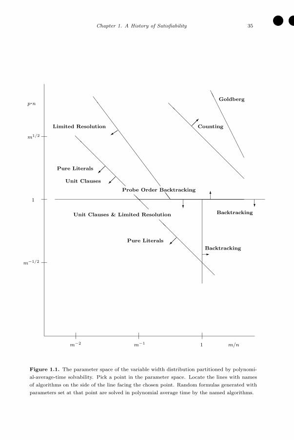
“p01c01˙his” — 2008/11/20 — 10:11 — page 35 — #35�

�

�

�

�

�


��

��

��

��

��

��

��

��

��

��

��

��

��

��

��

�

��

��

��

��

��

��

��

��

��

��

��

��

�

�

��

��

��

�

��

m−1/2

1

m1/2

.p n

m−2 m−1 1 m/n

Goldberg

Counting

Backtracking

Backtracking

Pure Literals

Pure Literals

Limited Resolution

Unit Clauses

Unit Clauses & Limited Resolution

Probe Order Backtracking

Figure 1.1. The parameter space of the variable width distribution partitioned by polynomi-

al-average-time solvability. Pick a point in the parameter space. Locate the lines with names

of algorithms on the side of the line facing the chosen point. Random formulas generated with

parameters set at that point are solved in polynomial average time by the named algorithms.

�

�

“p01c01˙his” — 2008/11/20 — 10:11 — page 36 — #36�

�

�

�

�

�


- then, if an empty clause does not exist when no more resolutions are possible,do a full search for a solution. The conditions under which this algorithm runsin polynomial average time under random variable width expressions are toocomplex to be given here but they are represented by the regions in Figure 1.1below the lines labeled Limited Resolution [Fra86a] (1991).

If pure literal reductions are added to the algorithm analyzed by Goldbergthen polynomial average time is achieved in the Pure Literals region, consider-ably improving the result of Goldberg [PB85] (1985). But a better result, shownas the region bounded from above by the lines labeled Unit Clauses, is obtainedby performing unit propagation [Fra93] (1993) and is consistent with the empir-ically and theoretically demonstrated importance of unit propagation in DPLL

algorithms. Results for Search Rearrangement Backtracking [Pur83] (1983) aredisappointing (shown bounded by the two lines labeled Backtracking) but aslightly different variant in which only variables from positive clauses (a positive

clause contains only positive literals) are chosen for elimination (if there is no pos-itive clause, satisfiability is determined by assigning all unassigned variables thevalue 0), has spectacular performance as is shown by the line labeled Probe Or-

der Backtracking [PH97] (1997). The combination of probe order backtrackingand unit clauses yield polynomial average time for random (n,m, p)-CNF expres-sions at every point of the parameter space except for some points along the thinhorizontal region p · n = c · log(n).

By 1997, what Goldberg had set out to do in 1979, namely show DPLL haspolynomial average time complexity for variable width distributions, had beenaccomplished. The research in this area had some notable successes such as theanalysis of probe order backtracking which demonstrated that a slight algorithmicchange can have a major effect on perfomance. But, the fact that nearly everypoint in the parameter space is covered by an algorithm that has polynomial av-erage time complexity is rather disturbing, though, since there are many practicalapplications where SAT is considered extremely difficult. Largely for this reasonattention shifted to the constant width distribution and, by the middle of the1990s, research on the variable width distribution all but disappeared.

Constant width distribution

Franco and Paull (1983) in [FP83] (see [PRF87], 1987, for corrections) set out totest Goldberg’s result on other distributions. They formulated the constant widthdistribution and showed that for all k ≥ 3 and every fixed m/n > 0, with proba-bility 1− o(1), the algorithm analyzed by Goldberg takes an exponential numberof steps to report a result: that is, either to report all (“cylinders” of) models, orthat no model exists. They also showed that a random (n,m, k)-CNF expressionis unsatisfiable with probability tending to 1 when m/n > − ln(2)/ ln(1 − 2−k).For k = 3 this is m/n > 5.19.

Perhaps the first positive result using the constant width distribution waspresented in [CF86] (1986) where a non-backtracking, incremental assignmentalgorithm employing unit propagation, called UC, was shown to find a model withbounded probability when m/n < O(1) · 2k/k. This work introduced an analysistool called “clause-flows” analysis which was refined by Achlioptas [Ach01] (2001)using a theorem of Wormald [Wor95]. Analysis of clause flows via differentialequations was to be the basic analytic tool for most of the following results in

�

�

“p01c01˙his” — 2008/11/20 — 10:11 — page 37 — #37�

�

�

�

�

�


this area. In [CF90] (1990) it was shown that a generalization of unit propagation,called GUC, in which a variable from a “smallest” clause is chosen for assignmentfinds a model with probability 1 − o(1) when m/n < O(1) · 2k/k, k ≥ 4. Thiswas improved by Chvatal and Reed [CR92] (1992) who showed that GUC, withassignment rules relaxed if no unit or two literal clauses are present (called SC forshortest clause), finds a model with probability 1− o(1) when m/n < O(1) · 2k/k

for k ≥ 3.

Observe that the results of the previous two paragraphs show a gap betweenthe range m/n > ln(2)/ ln(1 − 2−k) ≈ 2k ln(2), where random expressions areunsatisfiable with high probability, and m/n < O(1) · 2k/k, where analyzed non-backtracking incremental assignment algorithms find models for random expres-sions with high probability. According to results of Friedgut (1999 - see Sec-tion 1.22) there is a sharp satisfiability threshold rk for every k ≥ 2 (it is stillnot known whether the threshold depends on n) and the results above show2k/k < rk < 2k ln(2). The question of the location of rk was pondered for quitesome time. Most people intuitively believed that rk was located near 2k ln(2)so the question became known as the ‘Why 2 k?’ problem (Pittel, 1999). Thiswas verified by Achlioptas, Moore, and Perez in [AM02, AP04] (2002,2004) whoshowed that rk = 2k ln(2) − O(k) by applying the second moment method to asymmetric variant of satisfiability, known as not-all-equal k-SAT (NAE-k-SAT).In NAE-k-SAT the question is whether, for a given CNF expression, there is asatisfying assignment whose complement is also a satisfying assignment. Obvi-ously, the class of k-CNF expressions satisfiable in NAE-k-SAT is a subset of theclass satisfiable in the traditional sense. Hence, for the purposes of finding thethreshold, NAE-k-SAT may be analyzed instead of k-SAT. The symmetric natureof NAE-k-SAT results in a low variance in the number of satisfying assignmentsand this makes the second moment method work.

Most interest, though, has centered on the case k = 3. It is believed, fromexperiment, that r3 ≈ 4.25. In [CF86] (1986) it is shown that UC finds a modelwith bounded probability when m/n < 8/3 = 2.66.. and, when combined with a“majority” rule (that is, choose a variable with the maximum difference betweenthe number of its positive and negative literals if unit propagation cannot beapplied), this improves to m/n < 2.9. Frieze and Suen [FS96] (1996) consideredSC and GUC and showed that for m/n < 3.003.., both heuristics succeed withpositive probability. Moreover, they proved that a modified version of GUC,called GUCB, which uses a limited form of backtracking, succeeds almost surelyfor the same range of m/n. Later, Achlioptas [Ach00] (2000) analyzed SC, mod-ified slightly to choose two variables at a time from a clause with two unfalsifiedliterals, for an improvement to m/n ≤ 3.145 with probability 1− o(1).

Nearly all the results above apply to myopic algorithms. A non-backtracking,variable assignment algorithm is called myopic [AS00] if, under the spectral co-alescence of states, the distribution of expressions corresponding to a particularcoalesced state can be expressed by its spectral components alone: that is, bythe number of clauses of width i, for all 1 ≤ i ≤ k, and the number of assignedvariables. Being myopic considerably assists an analysis by preserving statisticalindependence from one algorithmic step to the next. Unfortunately, in [AS00](2000) it is shown that no myopic algorithm can have good probabilistic perfor-

�

�

“p01c01˙his” — 2008/11/20 — 10:11 — page 38 — #38�

�

�

�

�

�


mance when m/n > 3.26. In the same paper it is shown that at least one myopicalgorithm almost surely finds a model if m/n < 3.26.

However, Kaporis et al. [KKL06] (2002) found a workaround to this “bar-rier” and analyzed a simple non-myopic greedy algorithm for Satisfiability. Theycontrol the statistical dependence problem by considering a different generatorof expressions such that probabilistic results also hold for random (n,m, 3)-CNFexpressions. Their result is that a greedy algorithm for satisfiability almost al-ways finds a model when m/n < 3.42. Similar algorithms have been shown tofind a model, almost always, when m/n < 3.52 [HS03, KKL04] (2003). With thisanalysis machinery in place, better results are expected.

Although most of the results of the previous paragraph were motivated bythreshold research (see Section 1.22), their analyses can influence algorithm de-velopment. It is hoped future probabilistic results will reveal new generally usefulsearch heuristics, or at least explain the mechanics of existing search heuristics.

Another analysis should be noted for the following non-myopic incrementalassignment algorithm: repeatedly assign values to pure literals to eliminate theclauses containing them. Broder, Frieze and Upfal [BFU93] (1993) proved thatthis algorithm almost always finds a model when m/n ≤ 1.63 and k = 3. Theyused Martingales to offset distribution dependency problems as pure literals areuncovered. Mitzenmacher [Mit97] (1997) showed that this bound is tight.

This section concludes with a history of results on algorithms which are in-tended to return certificates of unsatisfiability. Most of these results, all pes-simistic, are obtained for resolution. The best result, though, is obtained for analgorithm which finds lower bounds on the number of variable assignments thatmust be positive and the number that must be negative (via translation to twohitting set problems) and returns “unsatisfiable” if the sum is greater than thenumber of variables. This result is notable also because it makes use of a highlyunderused analysis tool in this area: eigenvalues. Recall that nearly all randomconstant width expressions are unsatisfiable if m/n > 2k ln(2).

Chvatal and Szemeredi obtained the earliest result on constant width distribu-tions, inspired by the work reported in Section 1.16, is that, with high probability,every resolution proof for a random unsatisfiable expression is exponentially longif limn,m→∞ m/n = f(k) > 2k ln(2) [CS88] (1988). The analysis shows the rootcause to be a property known as sparseness; which roughly indicates the numberof times pairs of clauses have a common literal or complementary pair of literals.When an expression is sparse any “moderately large” subset of its clauses mustcontain a “large” number of variables that occur exactly once in that subset.Sparsity forces the proof to have a large resolvent. But, almost all “short” reso-lution refutations contain no long clauses after eliminating all clauses satisfied bya particular small random partial assignment ρ. Moreover, resolution refutationsfor almost all unsatisfiable random (n,m, k)-CNF expressions with clauses satis-fied by ρ removed are sparse and, therefore, must have at least one high widthresolvent. Consequently, almost all unsatisfiable random expressions have longresolution refutations. Beame, Karp, Pitassi, Saks, Ben-Sasson, and Widgerson,among others, contributed ideas leading up to a concise understanding of thisphenomenon in [BP96] (1996), [BKPS98] (1998), [BSW01] (2001).

Despite considerable tweaking, the best we can say right now is that, with

�

�

“p01c01˙his” — 2008/11/20 — 10:11 — page 39 — #39�

�

�

�

�

�


probability tending to 0, the width of a shortest resolution proof is boundedby a polynomial in n when m/n > 2k ln(2) and limm,n→∞ m/n(k+2)/(4−ε) < 1,where ε is some small constant; and with probability tending to 1, the width ispolynomially bounded when limm,n→∞ m/n > (n/ log(n))k−2.

The failure of resolution has led to the development of a new technique byGoerdt for certifying unsatisfiability, mentioned above, that uses eigenvalues.In [GK01] this spectral technique is used to obtain bounds sufficient to showthat certifying unsatisfiability in polynomial time can be accomplished with highprobability when limm,n→∞ m/n > nk/2−1+o(1) which is considerably better thanresolution.

1.22. Probabilistic analysis: thresholds

Results of the 1980s (see Section 1.21) showed that, for random width k ex-pressions density, that is the ratio m/n, is correlated with certain interestingexpression properties. For example, it was shown that if m/n > 2k ln(2) then arandom instance is unsatisfiable with high probability and if m/n < O(1) · 2k/k

a random expression is satisfiable with high probability. So, it was clear that acrossover from probably unsatisfiable to probably satisfiable occurs as density ischanged. Early on it was speculated that “hardness” is directly related to thenature of crossover and this motivated the study of Satisfiability thresholds.

Actually, thresholds can apply to a multitude of properties, not just theproperty of a formula being satisfiable, so we give a general definition of thresholdhere. Let X = {x1, ..., xe} be a set of e elements. Let AX , a subset of the powerset of X (denoted 2X), be called a property. Call AX a monotone property if forany s ∈ AX , if s ⊂ s′, then s′ ∈ AX . Typically, a monotone property followsfrom a high-level description which applies to an infinite family of sets X. Forexample, let X = Ck,n be the set of all non-tautological, width k clauses thatcan be constructed from n variables. Thus e = 2k

(nk

)and any s ∈ 2Ck,n is a k-

CNF expression. Let UNSAT Ck,ndenote the property that a k-CNF expression

constructed from n variables is unsatisfiable. That is, any s ∈ UNSAT Ck,nhas

no model and any s ∈ 2Ck,n \ UNSAT Ck,nhas a model. If s ∈ UNSAT Ck,n

andc ∈ Ck,n such that c /∈ s, then s∪{c} ∈ UNSAT Ck,n

so the property UNSAT Ck,n

is monotone for k < n.For any 0 ≤ p ≤ 1 and any monotone property AX ⊂ 2X define

μp(AX) =∑

s∈AX

p|s|(1− p)e−|s|

to be the probability that a random set has the monotone property. For theproperty UNSAT Ck,n

(among others), s is a set of clauses, hence this probabilitymeasure does not match that for what we call random k-CNF expressions butcomes very close with p = m/(2k

(nk

)) ≈ m · k!/(2n)k.

Observe that μp(AX) is an increasing function of p.5 Let pc(X) denote that

5By illustration using UNSAT Ck,nthis reflects the fact that, as p increases, the average

number of clauses increases, so the probability that an expression has the UNSAT Ck,nproperty

increases.

�

�

“p01c01˙his” — 2008/11/20 — 10:11 — page 40 — #40�

�

�

�

�

�


value of p for which μp(AX) = c. The values of pc(X) change as the size of X

increases. There are two threshold types.AX is said to have a sharp threshold if, for any small, positive ε,

lim|X|→∞

(p1−ε(X)− pε(X))/p1/2(X) = 0.

AX is said to have a coarse threshold if, for any small, positive ε,

lim|X|→∞

(p1−ε(X)− pε(X))/p1/2(X) > 0.

From experiments based on the constant width distribution it appeared thatUNSAT Ck,n

has a sharp threshold and that the density at which the crossover oc-curs is a function of k. The so-called satisfiability threshold was therefore denotedby rk. In addition, as m/n is reduced significantly below (the experimentallydetermined) rk, algorithms of various types were observed to perform better andexpressions were more likely to be members of a polynomial time solvable class(see Section 1.19 for a description - an analysis of these classes is given later inthis section), and as m/n is increased significantly above rk various algorithmswere observed to perform better. But, in the neighborhood of rk random ex-pressions seemed to reach a point of maximum difficulty, at least for well-known,well-tried algorithms. Hence, the study of satisfiability thresholds was motivatedby a possible connection between the nature of hardness and the nature and lo-cation of thresholds. The constant width distribution has dominated this study,perhaps because expressions generated when parameters are set near rk tend tobe extremely difficult for known algorithms.

The conjecture of a sharp threshold can be traced to a paper by Mitchell,Selman, and Levesque [MSL92] (1992) where the “easy-hard-easy” phenomenonis pointed out. A possible explanation is given by Cheeseman in [CKT91] (1991)where long “backbones” or chains of inference are stated to be a likely cause asthe high density of well-separated “near-solutions” induced by backbones leadsto thrashing in search algorithms. Tremendous insight on this phenomenon camefrom the field of Statistical Mechanics [MZK+99b, MZ02] where the connectionbetween backbones and hardness was seen to be analogous to phase transitionsin spin glasses. Achlioptas advanced this further with a rigorous analysis as thisvolume was going to press.

The satisfiability threshold for random (n,m, 2)-CNF expressions was foundby Chvatal and Reed to be sharp with r2 = 1 [CR92] (1992) (it is historicallycorrect to note that Fernandez de la Vega [FdlV92] and Goerdt [Goe96] indepen-dently achieved the same result in the same year). The fact that (n,m, 2)-CNFexpressions can be solved in polynomial time [Coo71] means that there is a sim-

ple characterization for those instances which are unsatisfiable. Both [CR92]and [Goe96] make use of this characterization by focusing on the emergence ofthe “most likely” unsatisfiable random (n,m, 2)-CNF expressions.

For k > 2 the situation was much more difficult. The results of Section 1.21,some of which were bounded probability results, can be regarded as a history oflower bounds for the satisfiability threshold. Upper bounds were improved at aconsistent rate for a while, the most intense investigation focusing on the case

�

�

“p01c01˙his” — 2008/11/20 — 10:11 — page 41 — #41�

�

�

�

�

�


k = 3. Results due to Frieze and Suen [FS96] (1996), Kamath, Motwani, Palem,Spirakis [KMPS95] (1995), Fernandez de la Vega [EMFdlV97] (1997), Dubois,Boufkhad [DB97] (1997), Kirousis, Kranakis, Krizanc [KKK96] (1996), Kirousis,Kranakis, Krizanc, Stamatiou [KKKS98] (1998), Dubois [Dub01] (2001), andDubois, Boufkhad, Mandler [DBM00] (2002), containing many beautiful ideas,have brought the upper bound down to just over 4.5 for k = 3. From Section 1.21the lower bound for k = 3 is 3.52. From experiments, we expect r3 ≈ 4.25.

Friedgut [Fri99] (1999) proved that sharp satisfiability thresholds exist forrandom (n,m, k)-CNF expressions, thereby confirming the conjecture of [MSL92].This result immediately lifted all previously known and future constant probabil-ity bounds, to almost surely bounds. Friedgut’s result has left open the possibilitythat the satisfiability threshold is a function of both k and n and it is still notknown whether the satisfiability threshold depends on n, as weak as that depen-dency must be.

Monasson [MZK+99b, MZK+99a] (1999) and others conjectured that there isa strong connection between the “order” of threshold sharpness, that is whetherthe transition is smooth or discontinuous, and hardness. Consistent with this,using the characterization of unsatisfiable (n,m, 2)-CNF expressions mentionedabove, Bollobas et al. [BBC+01] (2001) completely determined the “scaling win-dow” for random (n,m, 2)-CNF expressions, showing that the transition fromsatisfiability to unsatisfiability occurs for m = n + λn2/3 as λ goes from −∞ to+∞. For some time scaling windows for various problems were consistent withMonasson’s conjecture (e.g. [CD99, CD03b]). But eventually the conjecture wasdisproved in [ACIM01] (2001) where it was found that the order of thresholdsharpness for the 1-in-k SAT problem, which is NP-complete, is the same as thatof 2-SAT.

On the other hand, the work of Creignou and Daude [CD03a] (2002), [CD04](2004) revealed the importance of minimal monotonic structures to the existenceof sharp transitions. An element s ∈ AX is said to be minimal if for all s′ ⊂ s,s′ ∈ 2X \ AX . Those results have been used, for example, to show the limita-tions of most succinctly defined polynomial-time solvable classes of expressions,such as those mentioned in Section 1.19. Using density m/n of (n,m, k)-CNFdistributions as a measure, thresholds for some classes of Section 1.19 have beendetermined: for example, a random (n,m, k)-CNF expression, k ≥ 3, is q-Hornwith probability tending to 1 if m/n < O(1)/(k2−k) and with probability tendingto 0 if m/n > O(1)/(k2− k) [FVG03, CDF05]. Except for the matched class, themonotonic structure analysis shows why the classes of Section 1.19, including q-Horn, SLUR, renameable Horn and many others, are weak: they are “vulnerable”to cyclic clause structures, the presence of any of these in an expression preventsit from having the polynomial-time solveable property. A random expression ismatched with probability tending to 1 if m/n < 0.64 [FVG03]: a result that addsperspective to the scope of most polynomial-time solveable classes.

Also of historical importance are results on 2 + p mixed random expressions:random expressions with width 2 and width 3 clauses, the p being the fraction ofwidth 3 clauses. This distribution was introduced in [KS94] (1994) to help un-derstand where random expressions get hard during search: if a search algorithmthat embodies unit propagation is presented with a (n,m, 3)-CNF expression, ev-

�

�

“p01c01˙his” — 2008/11/20 — 10:11 — page 42 — #42�

�

�

�

�

�


ery search node represents such a mixed expression with a particular value of p

so hardness for some range of p could translate to hardness for search. Experi-mental evidence suggested that for some pc, figured to be around 0.417, if p < pc

the width 3 clauses were effectively irrelevant to the satisfiability of a randomexpression but if p > pc the transition behavior was more like that of a randomwidth 3 expression. In [AKKK01] (2001) it was shown that 0.4 < pc < 0.696 andconjectured that pc = 0.4. In [ABM04] (2004) it was shown that a random 2 + p

mixed expression has a minimum exponential size resolution refutation (that in-cludes any DPLL algorithm) with probability 1−o(1) when the number of width2 clauses is less than ρn, ρ < 1, and p is any constant. Actually, the results of thispaper are quite far-ranging and provide new insights into the behavior of DPLL

algorithms as they visit search nodes that represent 2 + p expressions.

1.23. Stochastic Local Search

by Holger Hoos

Stochastic local search (SLS) is one of the most successfully and widely usedgeneral strategies for solving hard combinatorial problems. Early applications tooptimization problems date back to the to the 1950s (for example, see [Cro58,Flo56, Lin65]), and the Lin-Kernighan algorithm for the Traveling Salesman prob-lem [LK73] (1973) is still among the most widely known problem-specific SLSalgorithms. Two of the most prominent general SLS methods are Simulated An-nealing [KGV83] (1983) and Evolutionary Algorithms [FOW66, Hol75, Sch81](1966–1981).

SLS algorithms for SAT were first presented in 1992 by Gu [Gu92] and Selmanet al. [SLM92] (following earlier applications to Constraint Satisfaction [MJPL90]and MAX-SAT [HJ90]). Interestingly, both Gu and Selman et al. were apparentlyunaware of the MAX-SAT work, and Hansen and Jaumard and Minton et al.appear to have been unaware of each other’s work. The success of Selman et al.’sGSAT algorithm in solving various types of SAT instances more effectively thanDPLL variants of the day sparked considerable interest in the AI community,giving rise to a fruitful and active branch of SAT research. GSAT is based ona simple iterative best improvement method with static restarts; in each localsearch step, it flips the truth value of one propositional variable such that thenumber of unsatisfied clauses in the given CNF formula is maximally reduced.

Within a year, the original GSAT algorithm was succeeded by a numberof variants. These include HSAT [GW93], which uses a very limited form ofsearch memory to avoid unproductive cycling of the search process; GSAT withClause Weighting [SK93], which achieves a similar goal using dynamically chang-ing weights associated with the clauses of the given CNF formula; and GSAT withRandom Walk (GWSAT) [SK93], which hybridizes the “greedy” search methodunderlying GSAT with a simple random walk procedure (which had previouslybeen shown by Papadimitriou [Pap91] to solve satisfiable 2-CNF formulae almostcertainly in O(n2) steps).

Two relatively subtle modifications of GWSAT lead to the prominent (basic)WalkSAT algorithm [SKC94], which is based on the idea of selecting a currentlyunsatisfied clause in each step and satisfying that clause by flipping the value

�

�

“p01c01˙his” — 2008/11/20 — 10:11 — page 43 — #43�

�

�

�

�

�


assigned to one of its variables. Basic WalkSAT (also known as WalkSAT/SKC)was shown empirically to outperform GWSAT and most other GSAT variantsfor a broad range of CNF formulae; it is also somewhat easier to implement.Variants of WalkSAT that additionally use search memory, in particular Walk-SAT/Tabu [MSK97] (1997) and Novelty+ [Hoo98, Hoo99] (1998) – an extensionof the earlier Novelty algorithm of McAllester et al. [MSK97] – typically achieveeven better performance. Novelty+, which has been proven to solve satisfiableCNF formulae with arbitrarily high probability given sufficient time, was laterextended with an adaptive noise mechanism [Hoo02] (2002), and the resultingAdaptive Novelty+ algorithm is still one of the most effective SLS algorithms forSAT currently known.

Based on the same fundamental idea of dynamically changing clause weightsas GSAT with Clause Weighting, Wah et al. developed an approach known asDiscrete Lagrangian Method [SW98] (1998), whose later variants were shown tobe highly effective, particularly for solving structured SAT instances [WW99,WW00]. A conceptually related approach, which uses multiplicatively modifiedclause weights has been developed by Schuurmans et al. [SSH01] (2001) and laterimproved by Hutter et al. [HTH02] (2002), whose SAPS algorithm was, untilrecently, one of the state-of-the-art SLS algorithms for SAT.

A detailed survey of SLS algorithms for SAT up to 2004 can be found inChapter 6 of the book by Hoos and Stutzle [HS05]. Since then, a number ofnew algorithms have been developed, including Li and Huang’s G2WSAT [LH05](2005), which combines ideas from the GSAT and WalkSAT family of algorithms,and Ishtaiwi et al.’s DDFW algorithm [ITA+06] (2006), which uses a dynamicclause weight redistribution. In another line of work, Anbulagan et al. have re-ported results suggesting that by using a resolution-based preprocessing method,the performance of several state-of-the-art SLS algorithms for SAT can be furtherimproved [APSS05](2005).

SLS algorithms for SAT have also played an important role in theoreticalwork on upper bounds on worst-case time complexity for solving SAT on k-CNF formulae; this includes the previously mentioned random walk algorithmby Papadimitriou [Pap91] (1991) and later extensions by Schoning [Sch99] (1999)and Schuler et al. [SSW01] (2001).

1.24. Maximum Satisfiability

by Hantao Zhang

The problem of finding a truth assignment to the variables of a CNF expressionthat satisfies the maximum number of clauses possible is known as MaximumSatisfiability or MAX-SAT. If clauses have at most two literals each, the problemis known as MAX-2-SAT. The decision version of MAX-SAT and even MAX-2-SAT is NP-complete. Unfortunately, there is no polynomial time approximationscheme for MAX-SAT unless P = NP [AL97]. Because the MAX-SAT prob-lem is fundamental to many practical problems in Computer Science [HJ90] andElectrical Engineering [XRS02], efficient methods that can solve a large set ofinstances of MAX-SAT are eagerly sought.

�

�

“p01c01˙his” — 2008/11/20 — 10:11 — page 44 — #44�

�

�

�

�

�


1.24.1. MAX-SAT: Decision Algorithms

Many of the proposed methods for MAX-SAT are based on approximationalgorithms [DGH+02] (2002); some of them are based on branch-and-boundmethods [HJ90] (1990), [BF99] (1999), [BR99] (1999), [Hir00] (2000), [NR00](2000), [dGLMS03] (2003); and some of them are based on transforming MAX-SAT into SAT [XRS02] (2002), [ARMS02a] (2002).

Worst-case upper bounds have been obtained with respect to three parame-ters: the length L of the input formula (i.e., the number of literals in the input),the number m of the input’s clauses, and the number n of distinct variables oc-curring in the input. The best known bounds for MAX-SAT are O(L2m/2.36)and O(L2L/6.89) [BR99] (1999). The question of whether there exist exact al-gorithms with complexity bounds down to O(L2n) has been open and of greatinterest (see [Nie98] (1998), [AGN01] (2000), [GHNR03] (2003)) since an algo-rithm which enumerates all the 2n assignments and then counts the number oftrue clauses in each assignment would take time O(L2n). Recently, it has beenshown that a branch-and-bound algorithm can achieve O(b2n) complexity whereb is the maximum number of occurrences of any variable in the input. Typically,b � L/n.

The operation of the best branch-and-bound algorithms for MAX-SAT is sim-ilar to that of DPLL. Notable implementations are due to Wallace and Freuder(implemented in Lisp) [WF96] (1996), Gramm [Gra99] (1999), Borchers and Fur-man [BF99] (1999 - implemented in C and publicly available), Zhang, Shen, andManya [ZSM03] (2003), and Zhao and Zhang [ZZ04] (2004).

1.24.2. MAX-2-SAT: Decision Algorithms

MAX-2-SAT is important because a number of other NP-complete problemscan be reduced to it in a natural way, for example graph problems such asMaximum Cut and Independent Set [CCTW96] (1996), [MR99a]. For MAX-2-SAT, the best bounds have been improved from O(m2m/3.44) [BR99] (1999), toO(m2m/2.88) [NR00] (2000), and recently to O(m2m/5) [GHNR03] (2003). The re-cent branch-and-bound algorithm cited above results in a bound of O(n2n) sinceb ≤ 2n. When m = 4n2 the bound is O(

√m1.414

√m), which is substantially

better than the result reported in [GHNR03].

For random 2-CNF formulas satisfiability thresholds have been found as fol-lows:

Theorem [CGHS04] :

1. For c < 1, K(n, cn) = Θ(1/n).2. For c large,

(0.25c− 0.343859√

c + O(1))n ≥ K(n, cn) ≥ (0.25c− 0.509833√

c)n.

3. For any fixed ε > 0, 13ε3n ≥ K(n, (1 + ε)n).

�

�

“p01c01˙his” — 2008/11/20 — 10:11 — page 45 — #45�

�

�

�

�

�


In the above theorem, ≥ is a standard asymptotic notation: f(n) ≥ g(n) meansthat f is greater than or equal to g asymptotically , that is, f(n)/g(n) ≥ 1 whenn goes to infinity, although it may be that f(n) < g(n) even for arbitrarily largevalues of n.

1.25. Nonlinear formulations

by Miguel Anjos

The nonlinear formulations for SAT are based on the application of the fundamen-tal concept of lift-and-project for constructing tractable continuous relaxations ofhard binary (or equivalently, Boolean) optimization problems. The applicationof continuous relaxations to binary optimization dates back at least to Lovasz’sintroduction of the so-called theta function as a bound for the stability number ofa graph [Lov79]. More generally, the idea of liftings for binary optimization prob-lems has been proposed by several researchers, and has led to different general-purpose frameworks. Hierarchies based on linear programming relaxations in-clude the lift-and-project method of Balas, Ceria and Cornuejols [BCC93], thereformulation-linearization technique of Sherali and Adams [SA90], and the matrix-cuts approach of Lovasz and Schrijver [LS91]. Researchers in the SAT com-munity have studied the complexity of applying some of these techniques, andgeneralizations thereof, to specific classes of SAT problems (see the recent pa-pers [BOGH+03, GHP02a, GHP02b]).

While the aforementioned techniques use linear programming relaxations, therecent Lasserre hierarchy is based on semidefinite programming relaxations [Las00,Las02]. (Semidefinite constraints may also be employed in the Lovasz-Schrijvermatrix-cuts approach, but in a different manner from that of the Lasserre paradigm.)A detailed analysis of the connections between the Sherali-Adams, Lovasz-Schrijver,and Lasserre frameworks was done by Laurent [Lau03]. In particular, Laurentshowed that the Lasserre framework is the tightest among the three.

Semidefinite programming (SDP) refers to the class of optimization problemswhere a linear function of a symmetric matrix variable X is optimized subjectto linear constraints on the elements of X and the additional constraint that X

must be positive semidefinite. This includes linear programming problems as aspecial case, namely when all the matrices involved are diagonal. The fact thatSDP problems can be solved in polynomial-time to within a given accuracy followsfrom the complexity analysis of the ellipsoid algorithm (see [GLS93]). A variety ofpolynomial time interior-point algorithms for solving SDPs have been proposedin the literature, and several excellent solvers for SDP are now available. TheSDP webpage [Hel] and the books [dK02, WSVe00] provide a thorough coverageof the theory and algorithms in this area, as well as a discussion of several appli-cation areas where semidefinite programming researchers have made significantcontributions. In particular, SDP has been very successfully applied in the de-velopment of approximation algorithms for several classes of hard combinatorialoptimization problems, including maximum-satisfiability (MAX-SAT) problems.

A σ-approximation algorithm for MAX-SAT is a polynomial-time algorithmthat computes a truth assignment such that at least a proportion σ of the clausesin the MAX-SAT instance are satisfied. The number σ is the approximation ratio

�

�

“p01c01˙his” — 2008/11/20 — 10:11 — page 46 — #46�

�

�

�

�

�


or guarantee. For instance, the first approximation algorithm for MAX-SAT isa 1

2 -approximation algorithm due to Johnson [Joh74]: given n values πi ∈ [0, 1],the algorithm sets the ith Boolean variable to 1 independently and randomlywith probability πi; the resulting total expected weight of the satisfied clausesis 1

2 . Unless P=NP, there is a limit to the approximation guarantees that canbe obtained. Indeed, Hastad [Has01] proved that unless P=NP , for any ε > 0,there is no (21

22 + ε)-approximation algorithm for MAX-2-SAT, and no (78 + ε)-

approximation algorithm for MAX-SAT.

The most significant breakthrough was by Goemans and Williamson [GW95]who proposed an SDP-based 0.87856-approximation algorithm for MAX-2-SAT.The key to their analysis is the ingenious use of a randomly generated hyperplaneto extract a binary solution from the set of n-dimensional vectors defined by thesolution of the SDP relaxation. The randomized hyperplane rounding procedurecan be formally de-randomized using the techniques in [MR99b].

A further significant improvement was achieved by Feige and Goemans [FG95]who proposed a 0.931-approximation algorithm for MAX-2-SAT. There are twokey innovations introduced by Feige and Goemans. The first one is that theytighten the SDP relaxation of Goemans and Williamson by adding the

(n3

)triangle

inequalities. From the optimal solution of this strengthened SDP relaxation, theysimilarly obtain a set of vectors, but instead of applying the random hyperplanerounding technique to these vectors directly, they use them to generate a set ofrotated vectors to which they then apply the hyperplane rounding.

Karloff and Zwick [KZ97] proposed a general construction of SDP relaxationsfor MAX-k-SAT. Halperin and Zwick [HZ01] consider strengthened SDP relax-ations for MAX-k-SAT, and specifically for MAX-4-SAT, they studied severalrounding schemes, and obtained approximation algorithms that almost attainthe theoretical upper bound of 7

8 . Most recently, Asano and Williamson [AW02]have combined ideas from several of the aforementioned approaches and obtaineda 0.7846-approximation algorithm for general MAX-SAT.

For the decision version of SAT, the first SDP-based approach is the Gap re-laxation of de Klerk, van Maaren, and Warners [dKvMW00, dKvM03]. This SDPrelaxation was inspired by the work of Goemans and Williamson as well as bythe concept of elliptic approximations for SAT instances. These approximationswere first proposed in [vM99] and were applied to obtain effective branching rulesas well as to recognize certain polynomially solvable classes of SAT instances.The idea behind the elliptic approximations is to reformulate a SAT formula onn boolean variables as the problem of finding a ±1 (hence binary) n-vector in anintersection of ellipsoids in Rn. Although it is difficult to work directly with in-tersections of ellipsoids, it is possible to relax the formulation to an SDP problem.The resulting SDP relaxation is called the Gap relaxation. This relaxation char-acterizes unsatisfiability for 2-SAT problems [dKvMW00]. More interestingly, italso characterizes satisfiability for a class of covering problems, such as mutilatedchessboard and pigeonhole instances. Rounding schemes and approximation guar-antees for the Gap relaxation, as well as its behaviour on (2 + p)-SAT problems,are studied in [dKvM03].

An elliptic approximation uses a quadratic representation of SAT formulas.More powerful relaxations can be obtained by considering higher-degree polyno-

�

�

“p01c01˙his” — 2008/11/20 — 10:11 — page 47 — #47�

�

�

�

�

�


mial representations of SAT formulas. The starting point is to define for eachclause a polynomial in ±1 variables that equals 0 if and only if the clause is sat-isfied by the truth assignment represented by the values of the binary variables.Thus, testing satisfiability of a SAT formula is reduced to testing whether thereare values x1, . . . , xn ∈ {−1, 1} such that for every clause in the instance, thecorresponding polynomial evaluated at these values equals zero.

We present two ways that SDP can be used to attempt to answer this ques-tion. One of them applies the Lasserre hierarchy mentioned above as follows. TheGap relaxation has its matrix variable in the space of (n+1)× (n+1) symmetricmatrices, and is thus a first lifting. To generalize this operation, we allow therows and columns of the SDP relaxations to be indexed by subsets of the dis-crete variables in the formulation. These larger matrices can be interpreted ashigher liftings. Applying directly the Lasserre approach to SAT, we would usethe SDP relaxations QK−1 (as defined in [Las00]) for K = 1, 2, . . . , n where thematrix variable of QK−1 has rows and columns indexed by all the subsets I with‖I‖ ≤ K (hence for K = 1, we obtain the matrix variable of the Gap relaxation).The results in [Las02] imply that for K = n, the resulting SDP relaxation charac-terizes satisfiability for every instance of SAT. However, this SDP has dimensionexponential in n. Indeed, the SDP problems quickly become far too large for prac-tical computation. This limitation motivated the study of partial higher liftings,where we consider SDP relaxations that have a much smaller matrix variable,as well as fewer linear constraints. The construction of such partial liftings forSAT becomes particularly interesting if we let the structure of the SAT instancespecify the structure of the SDP relaxation.

One of these partial liftings was proposed in [Anj05]. This construction con-siders all the monomials

∏i xi that appear in the instance’s satisfiability condi-

tions. An appropriate SDP relaxation is then defined where each row and columnof the matrix variable corresponds to one of these terms. The resulting matrix ishighly structured, and hence the SDP relaxation can be strengthened by addingsome constraints that capture this structure. The tradeoff involved in adding suchconstraints to the SDP problem is that as the number of constraints increases,the SDP problems become increasingly more demanding computationally. An-jos [Anj05] defines the SDP relaxation R3 by proposing to add a relatively smallnumber of these constraints, judiciously chosen so that it is possible to provethe following result: if R3 is infeasible, then the SAT instance is unsatisfiable;while if R3 is feasible, and Y is a feasible matrix such that rank(Y ) ≤ 3, thenthe SAT instance is satisfiable, and a model can be extracted from Y . Thus theSDP relaxation can prove either satisfiability or unsatisfiability of the given SATinstance. A more compact relaxation is obtained by defining the columns of thematrix variable using only the sets of odd cardinality. This yields the SDP relax-ation R2 [Anj04a], an intermediate relaxation between the Gap relaxation (callit R1 ) and R3. The names of the relaxations reflect their increasing strengthin the following sense: For k = 1, 2, 3, any feasible solution to the relaxationRk with rank at most k proves satisfiability of the corresponding SAT instance.Furthermore, the increasing values of k also reflect an improving ability to detectunsatisfiability, and an increasing computational time for solving the relaxation.

From the computational point of view, it is only possible to tackle relatively

�

�

“p01c01˙his” — 2008/11/20 — 10:11 — page 48 — #48�

�

�

�

�

�


small SAT instances (regardless of the choice of SDP relaxation) if branching isneeded [Anj04b]. However, when it does not require branching, the SDP approachcan be competitive. For instance, the SDP approach can successfully prove (with-out branching) the unsatisfiability of the hgen8 instances, one of which was thesmallest unsatisfiable instance that remained unsolved during the SAT competi-tions of 2003 and 2004.

A second way to test whether there is a set of ±1 values for which the clausepolynomials all equal zero was proposed by van Maaren and van Norden [vMvN05,vMvNH08]. They consider (among others) the aggregate polynomial obtained bysumming all the polynomials arising from clauses. This polynomial turns out to benon-negative on {−1, 1}n, and for x ∈ {−1, 1}n it equals the number of unsatisfiedclauses. (Hence, MAX-SAT is equivalent to the minimization of this polynomialover {−1, 1}n.) An SDP relaxation is obtained as follows. Suppose we are given acolumn vector β of monomials in the variables x1, . . . , xn and a polynomial p(x).Then p(x) can be written as a sum-of-squares (SOS) in terms of the elements ofβ if and only if there exists a matrix S � 0 such that βT Sβ = p [Par03]. If S issymmetric positive semidefinite, then S = WT W for some matrix W , and hencewe have an explicit decomposition of p as an SOS: βT Sβ = p ⇒ ||Wβ||22 = p.The resulting SDP problem is

max g

s.t. FBΦ (x)− g ≡ β

TSβ modulo IB

S � 0

where IB denotes the ideal generated by the polynomials x2k − 1, k = 1, . . . , n.

(The fact that each degree k polynomial that is non-negative on {−1, 1}n canbe expressed as an SOS modulo IB follows from the work of Putinar [Put93].)Note that since β is fixed, the equation F (x) − g = βT Sβ is linear in S and g,and hence this is an SDP problem. The SOS approach can thus be applied toobtain proofs of (un)satisfiability. For instance, it is straightforward to prove thatif there exists a monomial basis β and an ε > 0 such that FB(x) − ε is a SOSmodulo IB, then the underlying SAT formula is unsatisfiable.

For the SOS approach, different choices of the basis β result in differentSDP relaxations. Among the choices considered by van Maaren and van Nordenare the following: SOSGW is the relaxation obtained using the basis containing1, x1, . . . , xn ; SOSp is obtained using the basis containing 1, x1, . . . , xn, plus themonomial xk1

xk2for each pair of variables that appear together in a clause; SOSap

is obtained using the basis containing 1, x1, . . . , xn, plus the monomials xk1xk2

for all pairs of variables; SOSt is obtained using the basis containing 1, x1, . . . , xn,plus the monomial xk1

xk2xk3

for each triple of variables that appear together ina clause; and SOSpt is obtained using the basis containing 1, x1, . . . , xn, plus themonomial xk1

xk2for each pair of variables that appear together in a clause, plus

xk1xk2

xk3for each triple of variables that appear together in a clause.

The notation SOSGW is justified by the fact that SOSGW is precisely thedual of the SDP relaxation used by Goemans and Williamson in their seminalpaper [GW95]. van Maaren and van Norden prove that SOSGW gives the sameupper bound for MAX-2-SAT as the relaxation of Goemans and Williamson.They also show that for each triple xk1

xk2xk3

, adding the monomials xk1xk2

,

�

�

“p01c01˙his” — 2008/11/20 — 10:11 — page 49 — #49�

�

�

�

�

�


xk1xk3

, and xk2xk3

gives an SDP relaxation at least as tight as that obtained byadding the corresponding triangle inequality to the Goemans-Williamson relax-ation. Furthermore, they prove that the SDP relaxation SOSap is at least as tightas the Feige-Goemans relaxation, and that for every instance of MAX-3-SAT, theSDP relaxation SOSpt provides a bound at least as tight as the Karloff-Zwickrelaxation.

From the computational point of view, van Maaren and van Norden providecomputational results comparing several of these relaxations on instances of vary-ing sizes and varying ratios of number of clauses to number of variables. Theypropose rounding schemes for MAX-2-SAT and MAX-3-SAT based on SOSp andSOSt respectively, and present preliminary results comparing their performancewith the rounding schemes mentioned above. They also compare the performanceof the R3 relaxation with the SOS approach using either SOSt or SOSpt . Theirpreliminary results suggest that SOSpt offers the best performance.

The most recent result about the nonlinear approach is that the SDP ap-proach can explicitly characterize unsatisfiability for the well-known Tseitin in-stances on toroidal grid graphs. Consider a p× q toroidal grid graph and for eachnode (i, j), set the parameter t(i, j) = 0 or 1. Introduce a Boolean variable foreach edge, and for each node (i, j), define 8 clauses on the four variables adjacentto it as follows: if t(i, j) = 0, add all clauses with an odd number of negations;and if t(i, j) = 1, add all clauses with an even number of negations. It is clear thatthe SAT instance is unsatisfiable if and only if

∑(i,j) t(i, j) is odd. It is shown

in [Anj06] how to construct an SDP relaxation with matrix variable of dimension14pq and with 23pq − 1 linear equality constraints such that the SDP problemis infeasible if and only if the SAT instance is unsatisfiable. Therefore, for theseinstances, the SDP-based approach provides, in theory, an explicit certificate of(un)satisfiability, and therefore makes it possible to numerically compute such acertificate to within a given precision in polynomial time.

1.26. Pseudo-Boolean Forms

Let Bn be the set of binary vectors of length n. Mappings f :Bn �→ � arecalled pseudo-Boolean functions. Let V = {v1, v2, . . . , vn} be a set of n binaryvariables. Since there is a one-to-one correspondence between subsets of V andBn these functions are called set functions. There is a natural connection betweenpseudo-Boolean functions and binary optimization which has been exploited sincethe 1960s, especially following the seminal treatment of the topic by Hammerand Rudeanu in 1968 [HR68]. Areas impacted by pseudo-Boolean functions arediverse and include VLSI design (for example, [BGM88]), maximum satisfiability(for example, [Kar72]), clustering in statistics (for example, [Rao71]), economics(for example, [HS71]), graph theory (for example, [PR75]), and scheduling, amongmany others.

There are at least two important representations of pseudo-Boolean func-tions. All pseudo-Boolean functions may be uniquely represented as multi-linear

polynomials of the form

f(v1, v2, . . . , vn) = cf +∑S⊆V

cS

∏v∈S

v

�

�

“p01c01˙his” — 2008/11/20 — 10:11 — page 50 — #50�

�

�

�

�

�


where cS is some real number that depends on S and cf is a constant. The degreeof such a polynomial is the largest S for which cS = 0. A degree 1 polynomial iscalled linear , a degree 2 polynomial is called quadratic and so on.

Polynomials can also be written with non-negative constants using productsof literals instead of products of variables as follows:

f(v1, v2, . . . , vn) = cf +∑

S⊆V ∪V

cS

∏l∈S

l

where V = {¬v1,¬v2, . . . ,¬vn} is the set of negative literals associated with vari-ables (and positive literals) V and cS ≥ 0 with cS = 0 if there is a complementarypair {v,¬v} ∈ S. This is called the posiform representation of a pseudo-Booleanfunction. Although a posiform uniquely determines a pseudo-Boolean function, apseudo-Boolean function may be represented by more than one posiform. More-over, it is easy to compute a posiform from a polynomial representation but itmay be difficult to compute a unique polynomial representation corresponding toa given posiform. Because factors cS are non-negative, minimizing a posiform isessentially the same as maximizing the number of terms that are 0. Thus, theposiform representation is closely related to instances of maximum satisfiabilityand the problem of determining satisfiability of a Boolean formula may be viewedas testing whether the minimum of a posiform is equal to its constant term.

The optimization of a pseudo-Boolean function can be reduced in polynomialtime to the optimization of a quadratic pseudo-Boolean function [Ros72] (1972)by repeatedly substituting a new variable for a product of two variables and theaddition of constraints that force the new variable to take the value of the product.However, a posiform corresponding to a quadratic pseudo-Boolean function mayhave degree higher than 2.

The basic algorithm for finding the optimum value of a pseudo-Boolean func-tion was introduced in [HRR63b, HRR63a] (1963) and refined in [HR68] (1968).Although the algorithm has exponential complexity, special cases have been found,for example where the algorithm is fixed-parameter tractable [CHJ90] (1990). Anupper (lower) bound of a pseudo-Boolean function may be obtained by a term-by-term majorization (minorization) procedure which was introduced in [HHS84](1984). An algorithm for posiforms known as the DDT algorithm was developedin [BHS89] (1989).

In [CEI96] (1996) a variant of the Grobner basis algorithm was applied tosystems of posiforms restricted to modulo 2 arithmetic. The base operations ofthat algorithms were posiform addition, modulo 2, and variable multiplication.Application of such an operation is called a derivation. It was shown in [CEI96]that the algorithm uses a number of derivations that is guaranteed to be withina polynomial of the minimum number possible and that the minimum number ofderivations cannot be much greater than, and may sometimes be far less than,the minimum number needed by resolution.

More recently, conventional resolution-based SAT solvers have been general-ized to solve systems of linear polynomials. An early example is OPBDP [Bar95](1995). Notable advanced examples include PBS [ARMS02b] (2002) which has ad-vanced to PBS4 [AAR] (2005), Galena [CK03] (2003), and Pueblo [SS06] (2006).In [ES06] (2006) it is shown that translating linear polynomials to CNF clauses

�

�

“p01c01˙his” — 2008/11/20 — 10:11 — page 51 — #51�

�

�

�

�

�


and then solving with a conventional SAT solver is a viable alternative to spe-cialized pseudo-Boolean solvers although some expertise is needed to obtain thebest translations. The authors point out that translations might be the best ap-proach when problems are modeled with many clauses and a few pseudo-Booleancontraints.

1.27. Quantified Boolean formulas

by Hans Kleine Buning

The concept of quantified Boolean formulas (QBF) is an extension of proposi-tional logic that allows existential (∃) and universal (∀) quantifiers. The intendedsemantics of quantified Boolean formulas, without free variables, is that a uni-versally quantified formula ψ = ∀xφ is true if and only if for every assignment ofthe truth values 1 and 0 to the variable x, ψ is true. For existentially quantifiedformulas ψ = ∃xφ, ψ is true if and only if there is an assignment to x for whichφ is true. In the case of free variables, ψ is called satisfiable if there is a truthassignment to the free variables such that ψ is true. The satisfiability problemfor quantified Boolean formulas is often denoted as QSAT.

Most of the research has been done for formulas in prenex form, that is,formulas of the form Q1x1 . . . Qnxnφ, where Qi ∈ {∃,∀}, x1, . . . , xn are variables,and φ is a propositional formula called the matrix. By standard techniques, everyquantified Boolean formula can be transformed into a logically equivalent formulain prenex form. In the same way, by the well-known procedure for propositionalformulas, logically equivalent formulas with a CNF matrix or 3-CNF matrix canbe obtained. These classes are denoted as QCNF and Q3-CNF.

Quantified Boolean formulas with free variables are logically equivalent toBoolean functions. But, clearly, there is no polynomial p such that every n-aryBoolean function can be represented as a quantified Boolean formula of lengthp(n). However, for various applications, QBFs lead to shorter formulas in com-parison to propositional formulas. See, for example, [JB06].

The first papers on QBFs were motivated by questions arising from compu-tational complexity. Like SAT for NP, it has been shown in [MS73] that QSAT isone of the prominent PSPACE-complete problems. In a more detailed analysis,a strong relationship was shown between the satisfiability problem of formulaswith a fixed number of alternations of quantifiers and the polynomial–time hi-erarchy [MS72] where the polynomial–time hierarchy is defined as follows (k ≥ 0):

ΔP0 := ΣP

0 := ΠP0 := P

ΣPk+1 := NPΣP

k , ΠPk+1 := coΣP

k+1, ΔPk+1 := PΣP

k

For quantified Boolean formulas in prenex form, the prefix type is defined asfollows:

1. The prefix type of a propositional formula is Σ0 = Π0.2. Let Φ be a formula with prefix type Σn (Πn respectively), then the for-

mula ∀x1 . . . ∀xnΦ (∃x1 . . . ∃xnΦ respectively) is of prefix type Πn+1 (Σn+1

respectively).

�

�

“p01c01˙h

is”—

2008/11/20—

10:11—

page

52—

#52

�

�

�

�

�

�

52

Chapte

r1.

AH

istory

ofSatisfi

ability

1930

1950

1940

1900

1800

1850

1880

1700

−500

2000

1990

1980

1970

1960

2006 kr 2k

ProbabilisticAlgorithms

Spectralanalysis

Proof size vs.clause width

StochasticLocal Search

Novelty+ EquivalenceModels

Equivalence iscoNP−complete

Large proofsnearly always

Resolution/Complexity

EasyClasses

Large proofsfor PHCn

UpperBounds

ProbabilisticAnalysis

QBF

Survey Prop.Upper bounds

1st DPLL analysis Autarkies

Language syntax becomes richer

Boolean algebra, Venn diagrams

Appreciation of the power of applying algebra to scientific reasoningFirst logic system based on diagrams, wheels

Syllogistic logic, deduction

The first machine to solve problems in formal logic

Boolean algebra applied to circuit design

BDD definedBDD popularized

Consensus, circuit minimization

Model CheckingSimplifying ops

OBDD

BMD

CountingProbe order

Non−myopic algs

Random k−SATUC/GUC/SCMyopic limits

Minimal monotonic structuresSharp vs. Hard

NP−complete

Davis−Putnam ProcedureDPLLResolution lifted to 1st order logicExtended Resolution

Logicism, BegriffsschriftPrincipia MathematicaRelationship of Satisfiability to Computability

Precise notion of Satisfiability enunciatedGodel’s incompleteness theorem

..

CC−balanced

Extended Horn

q−HornLinear autarky

Horn (linear time)2−SAT (linear time)Renameable Horn2−SAT

HSATWalkSAT

GWSAT

Tabu

MAX−SAT

PSPACE−completeQ2−CNF, QHORN solvable

Q−unit−resolutionQ−resolution

ThresholdsBDD

Fig

ure

1.2

.T

imelin

e:

Som

enodeson

the

histo

rytre

e(c

ontin

ued

on

nextpage).

The

inte

ntio

n

isto

pro

vid

eso

me

persp

ectiv

eon

the

level

of

activ

ityin

apatic

ula

rare

adurin

ga

partic

ula

r

perio

d.

�

�

“p01c01˙h

is”—

2008/11/20—

10:11—

page

53—

#53

�

�

�

�

�

�

Chapte

r1.

AH

istory

ofSatisfi

ability

53

1930

1950

1940

1900

1800

1850

1880

1700

−500

2000

1990

1980

1970

1960

2006

Pseudo−Booleanfunctions

SAT SolversApplied toLinear Forms

MAX−SAT

No Approx. Scheme if P!=NPAwareness of Applications

Branch and BoundTranslation to SATThresholds

Simulated Annealing

Complexity & TransitionsSurvey Propagation Algorithm

Probabilistic Explanation

Survey Propagation Solver Refinements

RestartsIncremental Solvers

VSIDS HeuristicClausal LearningConflict AnalysisVDLIS HeuristicBreadth−First LookaheadBalanced Search SpaceJeroslow−Wang Heuristic

Reformulation−LinearizationMatrix−CutsSemi−Definite ProgrammingLift−and−Project

Applications ofContinuous Relaxationsto Boolean Optimization

{

0.7846 SDP Approx Alg for MAX−SAT0.931 SDP Approx Alg for MAX−2−SAT

Non−linear Relaxations

DDT Algorithm

Basic AlgorithmReduction to Quadratic Form

Upper Bounds

{

Fig

ure

1.2

.(c

ontin

ued)

Surv

ey

pro

pagatio

nis

show

non

the

chart

but

isnot

mentio

ned

in

the

text.

Ahisto

ryofalg

orith

ms

insp

ired

by

statistic

alm

ech

anic

sm

ay

be

found

inth

eSurv

ey

Pro

pagatio

nch

apte

rofth

isH

andbook.

�

�

“p01c01˙his” — 2008/11/20 — 10:11 — page 54 — #54�

�

�

�

�

�


It has been proved that for k ≥ 1, the satisfiability problem for formulas with pre-fix type Σk (Πk respectively) is ΣP

k -complete (ΠPk -complete respectively) [Sto77,

Wra77]. Since PSPACE =NPSPACE [Sav70], almost all quantified Boolean for-mula problems are solvable in PSPACE . For example, in propositional logic, theequivalence problem is coNP-complete, whereas for quantified Boolean formulas,the problem remains PSPACE-complete.

In addition to propositional formulas, a dichotomy theorem for quantifiedBoolean formulas has been established in [Sch73]. The idea was to classify classesof quantified Boolean formulas by means of a finite set of constraints, wherethe constraints are Boolean functions. The dichotomy theorem says that if theBoolean functions are equivalent to Horn formulas (anti-Horn formulas, 2-CNFformulas, XOR-CNF formulas respectively), then the satisfiability problems forthe quantified classes are in P, otherwise they are PSPACE-complete. As a con-sequence, the solvability of the satisfiability problem for Q2-CNF and QHORNfollows, where QHORN is the set of formulas, whose matrix is a Horn formula.Detailed proofs and extensions of the dichotomy theorem can be found, for exam-ple, in [Dal97, CKS92]. For formulas with fixed prefix type, further results havebeen shown in [Hem94].For Q2-CNF, the first linear-time algorithm for solving the satifiability problemhas been presented in [APT79]. For QHORN, the best known algorithm can befound in [KBKF95]. The latter algorithm requires not more than O(r · n) steps,where r is the number of universal variables and n is the length of the formula.

Not all the problems solvable in polynomial time for propositional formulasremain polynomial-time solvable for quantified formulas. For example, in contrastto the polynomial-time solvability of the equivalence problem for Horn formulas,the equivalence problem for quantified Horn formulas is coNP-complete [KBL99].

Instead of restrictions on the form of clauses, classes of quantified formulassatisfying some graph properties have been investigated. Examples are quantifiedversions of ordered binary decision diagrams (OBDDs) and free binary decisiondiagrams (FBDDs) (see, for example, [CMLBLM06]). For instance, the satisfia-bility problem for quantified FBDDs is PSPACE-complete.

Q-resolution is an extension of the resolution calculus for propositional for-mulas to quantified formulas. Q-unit-resolution was introduced in [KKBS88] andwas then generalized to Q-resolution in [KBKF95]. Here, a Q-unit clause containsat most one free or existentially quantified literal and arbitrarily many universalliterals. The idea of Q-resolution is to resolve only over complementary pairs ofexistential or free variables, combined with a careful handling of the universal lit-erals. Q-resolution is refutation complete and sound for QCNF. Similar to propo-sitional Horn formulas, Q-unit-resolution is refutation complete for QHORN, andalso for the class QEHORN. That is the set of formulas for which, after deletingthe universal literals in the matrix, the remaining matrix is a Horn formula. Thesatisfiability problem for that class remains PSPACE-complete [KKBF91].

A more functional view of the valuation of quantified Boolean formulas is theobservation that a formula is true if and only if for every existential variable y

there is a Boolean function fy(x1, . . . , xm) depending on the dominating universalvariables x1, . . . , xm, such that after replacing the existential variables y by theassociated functions fy(x1, . . . , xm) the formula is true. The set of such functions

�

�

“p01c01˙his” — 2008/11/20 — 10:11 — page 55 — #55�

�

�

�

�

�


is called a satsifiability model. For some classes of quantified Boolean formulas,the structure of the satisfiability models has been investigated. For example, sat-isfiable quantified Horn formulas have satisfiability models which consist of theconstants true and false or conjunctions of variables. For Q2-CNF, the modelsare constants or a literal [KBSZ07]. Instead of satisfiability models, one can askfor Boolean functions, such that after replacing the existentially quantified vari-ables with the functions, the formula is logically equivalent to the initial formula.These functions are called equivalence model. Equivalence models describe in acertain sense the internal dependencies of the formula. For example, quantifiedHorn formulas have equivalence models consisting of monotone functions. Bymeans of this result, it has been shown that every quantified Horn formula canbe transformed into an equivalent existentially quantified Horn formula in timeO(r · n), where r is the number of universal variables and n is the length of theformula [BKBZ05].

References

[AAR] F. Aloul and B. Al-Rawi. Pseudo-boolean solver, version 4. Avail-able: http://www.aloul.net/Tools/pbs4/.

[ABM04] D. Achlioptas, P. Beame, and M. Molloy. A sharp threshold inproof complexity yields lower bounds for satisfiability search. Jour-

nal of Computer and System Sciences, 68:238–268, 2004.[Ach00] D. Achlioptas. Setting 2 variables at a time yields a new lower

bound for random 3-sat. In 32nd ACM Symposium on Theory of

Computing, pages 28–37. Association for Computing Machinery,New York, 2000.

[Ach01] D. Achlioptas. Lower bounds for random 3-sat via differentialequations. Theoretical Computer Science, 265:159–185, 2001.

[ACIM01] D. Achlioptas, A. Chtcherba, G. Istrate, and C. Moore. The phasetransition in 1-in-k sat and nae 3-sat. In 12th ACM-SIAM Sympo-

sium on Discrete Algorithms, pages 721–722. Society for Industrialand Applied Mathematics, Philadelphia, 2001.

[AGN01] J. Alber, J. Gramm, and R. Niedermeier. Faster exact algorithmsfor hard problems: a parameterized point of view. Discrete Math-

ematics, 229(1-3):3–27, 2001.[Ake78] S. B. Akers. Binary decision diagrams. IEEE Transactions on

Computers, C-27(6):509–516, 1978.[AKKK01] D. Achlioptas, L. M. Kirousis, E. Kranakis, and D. Krizanc. Rigor-

ous results for random (2 + p)-sat. Theoretical Computer Science,265(1-2):109–129, 2001.

[AL86] R. Aharoni and N. Linial. Minimal non-two-colorable hypergraphsand minimal unsatisfiable formulas. Journal of Combinatorial

Theory, Series A, 43:196–204, 1986.[AL97] S. Arora and C. Lund. Hardness of approximation. In

D. Hochbaum, editor, Approximation algorithms for NP-hard

problems, chapter 10, pages 399–446. PWS Publishing Company,Boston, 1997.

http://www.aloul.net/Tools/pbs4/

�

�

“p01c01˙his” — 2008/11/20 — 10:11 — page 56 — #56�

�

�

�

�

�


[AM02] D. Achlioptas and C. Moore. The asymptotic order of the randomk-sat thresholds. In 43rd Annual Symposium on Foundations of

Computer Science, pages 779–788. IEEE Computer Society Press,Los Alamitos, CA, 2002.

[Anj04a] M. F. Anjos. On semidefinite programming relaxations for the sat-isfiability problem. Mathematical Methods of Operations Research,60(3):349–367, 2004.

[Anj04b] M. F. Anjos. Proofs of unsatisfiability via semidefinite program-ming. In D. Ahr, R. Fahrion, M. Oswald, and G. Reinelt, editors,Operations Research 2003, pages 308–315. Springer-Verlag, Berlin,2004.

[Anj05] M. F. Anjos. An improved semidefinite programming relax-ation for the satisfiability problem. Mathematical Programming,102(3):589–608, 2005.

[Anj06] M. F. Anjos. An explicit semidefinite characterization of satisfia-bility for tseitin instances on toroidal grid graphs. 2006.

[AP04] D. Achlioptas and Y. Peres. The threshold for random k-sat is2k(ln 2 + o(1)). Journal of the American Mathematical Society,17:947–973, 2004.

[APSS05] Anbulagen, D. N. Pham, J. Slaney, and A. Sattar. Old resolu-tion meets modern sls. In 12th National Conference on Artificial

Intelligence (AAAI ’05), pages 354–359. MIT Press, 2005.[APT79] B. Aspvall, M. F. Plass, and R. E. Tarjan. A linear-time algo-

rithm for testing the truth of certain quantified boolean formulas.Information Processing Letters, 8(3):121–132, 1979.

[ARMS02a] F. Aloul, A. Ramani, I. L. Markov, and K. A. Sakallah. Genericilp versus specialized 0-1 ilp: An update. In 2002 International

Conference on Computer-Aided Design (ICCAD ’02), pages 450–457. IEEE Computer Society Press, Los Alamitos, CA, 2002.

[ARMS02b] F. Aloul, A. Ramani, I. L. Markov, and K. A. Sakallah.Pbs: a backtrack search pseudo-boolean solver. In5th International Symposium on the Theory and Ap-

plications of Satisafiability Testing. 2002. Available:http://www.aloul.net/Papers/faloul sat02 pbs.pdf.

[AS00] D. Achlioptas and G. Sorkin. Optimal myopic algorithms for ran-dom 3-sat. In 41st Annual Symposium on Foundations of Com-

puter Science, pages 590–600. IEEE Computer Society Press, LosAlamitos, CA, 2000.

[Asp80] B Aspvall. Recognizing disguised nr(1) instances of the satisfiabil-ity problem. Journal of Algorithms, 1:97–103, 1980.

[AW02] T. Asano and D. P. Williamson. Improved approximation algo-rithms for max sat. Journal of Algorithms, 42(1):173–202, 2002.

[Bar69] M. E. Baron. A note on the historical development of logic dia-grams. The Mathematical Gazette: The Journal of the Mathemat-

ical Association, 53(384):113–125, 1969.[Bar95] P. Barth. A davis-putnam based enumeration algorithm for linear

pseudo-boolean optimization. Technical Report MPI-I-95-2-003,

http://www.aloul.net/Papers/faloul_sat02_pbs.pdf

�

�

“p01c01˙his” — 2008/11/20 — 10:11 — page 57 — #57�

�

�

�

�

�


Max Plank Institut fur Informatik, Saarbrucken, Germany, 1995.[BBC+01] B. Bollobas, C. Borgs, J. Chayes, J. H. Kim, and D. B. Wilson.

The scaling window of the 2-sat transition. Random Structures

and Algorithms, 18:201–256, 2001.[BC95] R. E. Bryant and Y.-A. Chen. Verification of arithmetic cir-

cuits with binary moment diagrams. In 32nd ACM/IEEE Design

Automation Conference, pages 535–541. IEEE Computer SocietyPress, Los Alamitos, CA, 1995.

[BCC93] E. Balas, S. Ceria, and G. Cornuejols. A lift-and-project cuttingplane algorithm for mixed 0-1 programs. Mathematical Program-

ming, 58(3, Ser. A):295–324, 1993.[BCCZ99] A. Biere, A. Cimatti, E. M. Clarke, and Y. Zhu. Symbolic model

checking without bdds. In 5th International Conference on Tools

and Algorithms for the Construction and Analysis of Systems

(TACAS ’99), volume 1579 of Lecture Notes in Computer Science,pages 193–207. Springer, New York, 1999.

[BCH90] E. Boros, Y. Crama, and P. L. Hammer. Polynomial-time inferenceof all valid implications for horn and related formulae. Annals of

Mathematics and Artificial Intelligence, 1:21–32, 1990.[BCHS94] E. Boros, Y. Crama, P. L. Hammer, and M. Saks. A complexity

index for satisfiability problems. SIAM Journal on Computing,23:45–49, 1994.

[BCM+92] J. R. Burch, E. M. Clarke, K. L. McMillan, D. L. Dill, and L. J.Hwang. Symbolic model checking: 1020 states and beyond. Infor-

mation and Computation, 98:142–170, 1992.[BF99] B. Borchers and J. Furman. A two-phase exact algorithm for max-

sat and weighted max-sat problems. Journal of Combinatorial

Optimization, 2(4):299–306, 1999.[BFG+93] R. I. Bahar, E. A. Frohm, C. M. Gaona, G. D. Hachtel, E. Macii,

A. Pardo, and F. Somenzi. Algebraic decision diagrams and theirapplications. In International Conference on Computer-Aided De-

sign, pages 188–191. IEEE Computer Society Press, Los Alamitos,CA, 1993.

[BFU93] A. Z. Broder, A. M. Frieze, and E. Upfal. On the satisfiability andmaximum satisfiability of random 3-cnf formulas. In 4th ACM-

SIAM Symposium on Discrete Algorithms, pages 322–330. Societyfor Industrial and Applied Mathematics, Philadelphia, 1993.

[BGM88] F. Barahona, M. Grotschel, and A. R. Mahjoub. An application ofcombinatorial optimization to statistical physics and circuit layoutdesign. Operations Research, 36:493–513, 1988.

[BHS89] E. Boros, P. L. Hammer, and X. Sun. The ddt method forquadratic 0-1 optimization. Technical Report RRR 39-1989, Rut-gers, the State University of New Jersey, 1989.

[BHS94] E. Boros, P. L. Hammer, and X. Sun. Recognition of q-horn formu-lae in linear time. Discrete Applied Mathematics, 55:1–13, 1994.

[BK04] T. Brueggemann and W. Kern. An improved local search algo-rithm for 3-sat. Theoretical Computer Science, 329:1–3, 2004.

�

�

“p01c01˙his” — 2008/11/20 — 10:11 — page 58 — #58�

�

�

�

�

�


[BKB92] M. Buro and H. Kleine Buning. Report on a sat competition.Technical report, 1992.

[BKBZ05] U. Bubeck, H. Kleine Buning, and X. Zhao. Quantifier rewritingand equivalence models for quantified horn formulas. In 8th Inter-

national Conference on the Theory and Applications of Satisafia-

bility Testing, volume 3569 of Lecture Notes in Computer Science,pages 386–392. Springer, New York, 2005.

[BKPS98] P. Beame, R. M. Karp, T. Pitassi, and M. Saks. On the complex-ity of unsatisfiability proofs for random k-cnf formulas. In 30th

Annual Symposium on the Theory of Computing, pages 561–571.Association for Computing Machinery, New York, 1998.

[BKS03] P. Beame, H. A. Kautz, and A. Sabharwal. On the power ofclause learning. In 18th International Joint Conference in Artifi-

cial Intelligence, pages 94–99. Morgan Kaufmann Publishers, SanFrancisco, CA, 2003.

[Bla37] A. Blake. Canonical Expressions in Boolean Algebra. PhD thesis,Department of Mathematics, University of Chicago, 1937.

[BOGH+03] J. Buresh-Oppenheim, N. Galesi, S. Hoory, A. Magen, andT. Pitassi. Rank bounds and integrality gaps for cutting planeprocedures. In 44th Annual Symposium on Foundations of Com-


[Bou76] R. T. Boute. The binary decision machine as a programmablecontroller. EUROMICRO Newsletter, 1(2):16–22, 1976.

[BP96] P. Beame and T. Pitassi. Simplified and improved resolution lowerbounds. In 37th Annual Symposium on Foundations of Computer

Science, pages 274–282. IEEE Computer Society Press, Los Alami-tos, CA, 1996.

[BR99] N. Bansal and V. Raman. Upper bounds for maxsat: Furtherimproved. In 7th International Symposium on Algorithms and

Computation, volume 1741 of Lecture Notes in Computer Science,pages 247–258. Springer, New York, 1999.

[BRB90] K. S. Brace, R. L. Rudell, and R. E. Bryant. Efficient implemen-tation of a bdd package. In 27th ACM/IEEE Design Automa-

tion Conference, pages 40–45. IEEE Computer Society Press, LosAlamitos, CA, 1990.

[Bro03] F. M. Brown. Boolean Reasoning. Dover Publications, Mineola,New York, 2003.

[Bry86] R. E. Bryant. Graph-based algorithms for boolean function ma-nipulation. IEEE Transactions on Computers, C-35(8):677–691,1986.

[Bry92] R. E. Bryant. Symbolic boolean manipulation with ordered binarydecision diagrams. ACM Computing Surveys, 24(3):293–318, 1992.

[BSIW04] E. Ben-Sasson, R. Impagliazzo, and A. Wigderson. Near opti-mal separation of tree-like and general resolution. Combinatorica,24(4):585–603, 2004.

[BSW01] E. Ben-Sasson and A. Wigderson. Short proofs are narrow - res-

�

�

“p01c01˙his” — 2008/11/20 — 10:11 — page 59 — #59�

�

�

�

�

�


olution made simple. Journal of the Association for Computing

Machinery, 48:149–169, 2001.[CBM90] O. Coudert, C. Berthet, and J. C. Madre. Verification of syn-

chronous sequential machines based on symbolic execution. InWorkshop on Automatic Verification Methods for Finite State Sys-

tems, volume 407 of Lecture Notes in Computer Science, pages365–373. Springer, New York, 1990.

[CCK+94] M. Conforti, G. Cornuejols, A. Kapoor, K. Vuskovic, and M. R.Rao. Balanced matrices. In J.R. Birge and K.G. Murty, editors,Mathematical Programming: State of the Art. Braun-Brumfield,United States, 1994.

[CCTW96] J. Cheriyan, W. H. Cunningham, L. Tuncel, and Y. Wang. A linearprogramming and rounding approach to max 2-sat. In DIMACS

Series in Discrete Mathematics and Theoretical Computer Science,volume 26, pages 395–414. DIMACS, Rutgers, the state Universityof New Jersey, 1996.

[CD99] N. Creignou and H. Daude. Satisfiability threshold for random xor-cnf formulas. Discrete Applied Mathematics, 96-97:41–53, 1999.

[CD03a] N. Creignou and H. Daude. Generalized satisfiability problems:minimal elements and phase transitions. Theoretical Computer

Science, 302(1-3):417–430, 2003.[CD03b] N. Creignou and H. Daude. Smooth and sharp thresholds for

random k-xor-cnf satisfiability. Theoretical Informatics and Ap-

plications, 37(2):127–148, 2003.[CD04] N. Creignou and H. Daude. Combinatorial sharpness criterion and

phase transition classification for random csps. Information and

Computation, 190(2):220–238, 2004.[CDF05] N. Creignou, H. Daude, and J. Franco. A sharp threshold for the

renameable horn and q-horn properties. Discrete Applied Mathe-

matics, 153:48–57, 2005.[CEI96] M. Clegg, J. Edmonds, and R. Impagliazzo. Using the groebner

basis algorithm to find proofs of unsatisfiability. In 28th Annual

ACM Symposium on the Theory of Computing, pages 174–183.Association for Computing Machinery, New York, 1996.

[CF86] M.-T. Chao and J. Franco. Probabilistic analysis of two heuris-tics for the 3-satisfiability problem. SIAM Journal on Computing,15:1106–1118, 1986.

[CF90] M.-T. Chao and J. Franco. Probabilistic analysis of a gener-alization of the unit-clause literal selection heuristics for the k-satisfiability problem. Information Sciences, 51:289–314, 1990.

[CGGT97] A. Cimatti, E. Giunchiglia, P. Giunchiglia, and P. Traverso. Plan-ning via model checking: a decision procedure for ar. In 4th Euro-

pean Conference on Recent Advances in AI Planning (ECP ’97),volume 1348 of Lecture Notes in Computer Science, pages 130–142.Springer, New York, 1997.

[CGHS04] D. Coppersmith, D. Gamarnik, M. T. Hajiaghayi, and G. B.Sorkin. Random max sat, random max cut, and their phase tran-

�

�

“p01c01˙his” — 2008/11/20 — 10:11 — page 60 — #60�

�

�

�

�

�


sitions. Random Structures and Algorithms, 24(4):502–545, 2004.[CH91] V. Chandru and J. N. Hooker. Extended horn sets in proposi-

tional logic. Journal of the Association for Computing Machinery,38:205–221, 1991.

[Cha84] R. Chandrasekaran. Integer programming problems for which asimple rounding type of algorithm works. In W. Pulleyblank, edi-tor, Progress in Combinatorial Optimization, pages 101–106. Aca-demic Press Canada, Toronto, Ontario, Canada, 1984.

[CHJ90] Y. Crama, P. Hansen, and B. Jaumard. The basic algorithm forpseudo-boolean programming revisited. Theoretical Computer Sci-

ence, 29(2-3):171–185, 1990.[Chu36] A. S. Church. Formal definitions in the theory of ordinal numbers.

Fundamental Mathematics, 28:11–21, 1936.[CK03] D. Chai and A. Kuehlmann. A fast psudo-boolean constraint

solver. In 40th ACM/IEEE Design Automation Conference, pages830–835. IEEE Computer Society Press, Los Alamitos, CA, 2003.

[CKS92] N. Creignou, S. Khanna, and M. Sudan. Complexity classifica-

tions of Boolean constraint satisfaction problems. Monographs onDiscrete Applied Mathematics. Society for Industrial and AppliedMathematics, Philadelphia, 1992.

[CKT91] P. Cheeseman, B. Kanefsky, and W. M. Taylor. Where the reallyhard problems are. In 12th International Joint Conference on Ar-

tificial Intelligence, pages 331–340. Morgan Kaufmann Publishers,San Francisco, CA, 1991.

[CM90] O. Coudert and J. C. Madre. A unified framework for the for-mal verification of sequential circuits. In International Conference

on Computer-Aided Design (ICCAD ’90), pages 126–129. IEEEComputer Society Press, Los Alamitos, CA, 1990.

[CMFT93] O. Coudert, J. C. Madre, H. Fraisse, and H. Touati. Implicit primecover computation: an overview. In 1st Workshop on Synthesis

And System Integration of Mixed Information technologies. Nara,Japan, 1993.

[CMLBLM06] S. Coste-Marquis, D. Le Berre, F. Letombe, and P. Marquis. Com-plexity results for quantified boolean formulae based on completepropositional languages. Journal on Satisfiability, Boolean Model-

ing and Computation, 1:61–88, 2006.[Coo71] S. A. Cook. The complexity of theorem-proving procedures. In 3rd

Annual ACM Symposium on Theory of Computing, pages 151–158.Association for Computing Machinery, New York, 1971.

[Cou94] O. Coudert. Two-level logic minimization: an overview. Integra-

tion, 17(2):97–140, 1994.[CR92] V. Chvatal and B. Reed. Mick gets some (the odds are on his side).

In 33rd Annual Symposium on Foundations of Computer Science,pages 620–627. IEEE Computer Society Press, Los Alamitos, CA,1992.

[Cro58] G. A. Croes. A method for solving traveling salesman problems.Operations Research, 6:791–812, 1958.

�

�

“p01c01˙his” — 2008/11/20 — 10:11 — page 61 — #61�

�

�

�

�

�


[CS88] V. Chvatal and E. Szemeredi. Many hard examples for resolution.Journal of the Association for Computing Machinery, 35:759–768,1988.

[Dal97] V. Dalmau. Some dichotomy theorems on constant free booleanformulas. Technical Report TR-LSI-97-43-R, Universitat Polytech-nica de Catalunya, 1997.

[Dav01] M. Davis. The early history of automated deduction. In A. Robin-son and A. Voronkov, editors, Handbook of Automated Deduction.MIT Press, 2001.

[DB97] O. Dubois and Y. Boufkhad. A general upper bound for the satisfi-ability threshold of random r-sat formulae. Journal of Algorithms,24:395–420, 1997.

[DBM00] O. Dubois, Y. Boufkhad, and J. Mandler. Typical random 3-sat formulae and the satisfiability threshold. In 11th ACM-SIAM

Symposium on Discrete Algorithms, pages 124–126. Society forIndustrial and Applied Mathematics, Philadelphia, 2000.

[DG84] W. F. Dowling and J. H. Gallier. Linear-time algorithms for testingthe satisfiability of propositional horn formulae. Journal of Logic

Programming, 1:267–284, 1984.[DGH+02] E. Dantsin, A. Goerdt, E. A. Hirsch, R. Kannan, J. Kleinberg,

C. Papadimitriou, P. Raghavan, and U. Schoning. A determin-istic (2 − 2/(k + 1))n algorithm for k-sat based on local search.Theoretical Computer Science, 289:69–83, 2002.

[dGLMS03] S. de Givry, J. Larrosa, P. Meseguer, and T. Schiex. Solving max-sat as weighted csp. In 9th International Conference on Principles

and Practice of Constraint Programming (CP 2003), volume 2833of Lecture Notes in Computer Science, pages 363–376. Springer,New York, 2003.

[dK02] E. de Klerk. Aspects of Semidefinite Programming, volume 65 ofApplied Optimization. Kluwer Academic Publishers, Dordrecht,2002.

[DK03] R. Damiano and J. Kukula. Checking satisfiability of a conjunc-tion of bdds. In 40th ACM/IEEE Design Automation Conference,pages 818–823. IEEE Computer Society Press, Los Alamitos, CA,2003.

[dKvM03] E. de Klerk and H. van Maaren. On semidefinite programmingrelaxations of (2 + p)-sat. Annals of Mathematics and Artificial

Intelligence, 37(3):285–305, 2003.[dKvMW00] E. de Klerk, H. van Maaren, and J. P. Warners. Relaxations of the

satisfiability problem using semidefinite programming. Journal of

Automated Reasoning, 24(1-2):37–65, 2000.[DLL62] M. Davis, G. Logemann, and D. Loveland. A machine program for

theorem proving. Communications of the ACM, 5:394–397, 1962.[DP58] M. Davis and H. Putnam. Computational methods in the propo-

sitional calculus. unpublished report, Rensselaer Polytechnic In-stitute, 1958.

[DP60] M. Davis and H. Putnam. A computing procedure for quantifica-

�

�

“p01c01˙his” — 2008/11/20 — 10:11 — page 62 — #62�

�

�

�

�

�


tion theory. Journal of the Association for Computing Machinery,7(3):201–215, 1960.

[Dub01] O. Dubois. Upper bounds on the satisfiability threshold. Theoret-

ical Computer Science, 265:187–197, 2001.[DW04] E. Dantsin and A. Wolpert. Derandomization of schuler’s algo-

rithm for sat. In 6th International Conference on the Theory and

Applications of Satisfiability Testing, volume 2919 of Lecture Notes

in Computer Science, pages 69–75. Springer, New York, 2004.[DW05] E. Dantsin and A. Wolpert. An improved upper bound for sat. In

8th International Conference on the Theory and Applications of

Satisfiability Testing, volume 3569 of Lecture Notes in Computer

Science, pages 400–407. Springer, New York, 2005.[EIS76] S. Even, A. Itai, and A. Shamir. On the complexity of timetable

and multi-commodity flow problems. SIAM Journal on Comput-

ing, 5:691–703, 1976.[EMFdlV97] A. El Maftouhi and W. Fernandez de la Vega. On random 3-sat.

Laboratoire de Recherche en Informatique, Universite Paris-Sud,France, 1997.

[ES06] Niklas Een and Niklas Sorensson. Translating pseudo-boolean con-straints into sat. Journal on Satisfiability, Boolean Modeling and

Computation, 2:1–25, 2006.[FdlV92] W. Fernandez de la Vega. On random 2-sat. Manuscript, 1992.

[FG95] U. Feige and M. Goemans. Approximating the value of two proverproof systems, with applications to max 2sat and max dicut. In3rd Israel Symposium on the Theory of Computing and Systems,pages 182–189. IEEE Computer Society Press, Los Alamitos, CA,1995.

[FH89] J. Franco and Y. C. Ho. Probabilistic performance of heuristic forthe satisfiability problem. Discrete Applied Mathematics, 22:35–51, 1988/89.

[FKS+04] J. Franco, M. Kouril, J. Schlipf, J. Ward, S. Weaver, M. Dransfield,and W. M. Vanfleet. Sbsat: a state-based, bdd-based satisfiabilitysolver. In 6th International Conference on the Theory and Appli-

cations of Satisfiability Testing, volume 2919 of Lecture Notes in

Computer Science, pages 398–410. Springer, New York, 2004.[Flo56] M. M. Flood. The traveling salesman problem. Operational Re-

search, 4(1):61–75, 1956.[FOW66] L. J. Fogel, A. J. Owens, and M. J. Walsh. Artificial Intelligence

Through Simulated Evolution. John Wiley & Sons, New York,1966.

[FP83] J. Franco and M. Paull. Probabilistic analysis of the davis-putnamprocedure for solving the satisfiability problem. Discrete Applied

Mathematics, 5:77–87, 1983.[Fra86a] J. Franco. Elimination of infrequent variables improves average

case performance of satisfiability algorithms. SIAM Journal on

Computing, 20:103–106, 1986.[Fra86b] J. Franco. On the probabilistic performance of algorithms for the

�

�

“p01c01˙his” — 2008/11/20 — 10:11 — page 63 — #63�

�

�

�

�

�


satisfiability problem. Information Processing Letters, 23:103–106,1986.

[Fra93] J. Franco. On the occurrence of null clauses in random instancesof satisfiability. Discrete Applied Mathematics, 41:203–209, 1993.

[Fre95] J. W. Freeman. Improvements to Propositional Satisfiability

Search Algorithms. PhD thesis, University of Pennsylvania, USA,1995.

[Fri99] E. Friedgut. Sharp thresholds of graph properties, and the k-sat problem. Journal of the American Mathematical Society,12(4):1017–1054, 1999. with an appendix by J. Bourgain.

[FS96] A. M. Frieze and S. Suen. Analysis of two simple heuristics ona random instance of k-sat. Journal of Algorithms, 20:312–355,1996.

[FVG03] J. Franco and A. Van Gelder. A perspective on certain polynomialtime solvable classes of satisfiability. Discrete Applied Mathemat-

ics, 125(2–3):177–214, 2003.[Gal77] Z. Galil. On the complexity of regular resolution and the davis-

putnam procedure. Theoretical Computer Science, 4:23–46, 1977.[Gar58] M. Gardner. Logic Machines and Diagrams. McGraw-Hill, New

York, 1958.[Gel59] H. Gelernter. Realization of a geometry-theorem proving ma-

chine. In International Conference on Information Processing,pages 273–282. UNESCO House, 1959.

[GHNR03] J. Gramm, E. A. Hirsch, R. Niedermeier, and P. Rossmanith. Newworst-case upper bounds for max-2-sat with application to max-cut. Discrete Applied Mathematics, 130(2):139–155, 2003.

[GHP02a] D. Grigoriev, E. A. Hirsch, and D. V. Pasechnik. Complexity ofsemialgebraic proofs. Moscow Mathematics Journal, 2(4):647–679,2002.

[GHP02b] D. Grigoriev, E. A. Hirsch, and D. V. Pasechnik. Exponentiallower bound for static semi-algebraic proofs. In 29th International

Colloquium on Automata, Languages and Programming (ICALP

’02), volume 2380 of Lecture Notes in Computer Science, pages257–268. Springer, New York, 2002.

[Gil60] P. Gilmore. A proof method for quantification theory: its justifica-tion and realization. IBM Journal of Research and Development,4:28–35, 1960.

[GK01] A. Goerdt and M. Krivelevich. Efficient recognition of randomunsatisfiable k-sat instances by spectral methods. In 18th Sym-

posium on Theoretical Aspects of Computer Science (STACS’01),volume 2010 of Lecture Notes in Computer Science, pages 294–304.Springer, New York, 2001.

[GLS93] M. Grotschel, L. Lovasz, and A. Schrijver. Geometric Algorithms

and Combinatorial Optimization. Algorithms and Combinatorics,Vol. 2. Springer-Verlag, Berlin, 1993.

[Goe96] A. Goerdt. A threshold for unsatisfiability. Journal of Computer

System Science, 53:469–486, 1996.

�

�

“p01c01˙his” — 2008/11/20 — 10:11 — page 64 — #64�

�

�

�

�

�


[Gol79] A. Goldberg. On the complexity of the satisfiability problem. In4th Workshop on Automated Deduction, pages 1–6. Austin, Texas,1979.

[GPB82] A. Goldberg, P. W. Purdom, and C. Brown. Average time analy-sis of simplified davis-putnam procedures. Information Processing

Letters, 15:72–75, 1982.[Gra99] J. Gramm. Exact algorithms for max2sat and their applications.

Diplomarbeit, Universitat Tubingen, 1999.[Gu92] J. Gu. Efficient local search for very large scale satisfiability prob-

lems. SIGART Bulletin, 3(1):8–12, 1992.[GW93] I. P. Gent and T. Walsh. An empirical analysis of search in gsat.

Journal of Artificial Intelligence Research, 1:47–59, 1993.[GW95] M. X. Goemans and D. P. Williamson. Improved approxima-

tion algorithms for maximum cut and satisfiability problems usingsemidefinite programming. Journal of the Association for Com-

puting Machinery, 42(6):1115–1145, 1995.[GZ03] J. F. Groote and H. Zantema. Resolution and binary decision dia-

grams cannot simulate each other polynomially. Discrete Applied

Mathematics, 130(2):157–171, 2003.[Hak85] A. Haken. The intractability of resolution. Theoretical Computer

Science, 39:297–308, 1985.[Has01] J. Hastad. Some optimal inapproximability results. Journal of the

Association for Computing Machinery, 48:798–859, 2001.[HBBM97] Y. Hong, P. A. Beerel, J. R. Burch, and K. L. McMillan. Safe

bdd minimization using don’t cares. In 34th ACM/IEEE Design

Automation Conference, pages 208–213. IEEE Computer SocietyPress, Los Alamitos, CA, 1997.

[HD66] C. Herlinus and C. Dasypodius. Analyseis Geometricae Sex Libo-

rum Euclidis. J. Rihel, Strausbourg, 1566.[HD04] J. Huang and A. Darwiche. Toward good elimination orders for

symbolic sat solving. In 16th IEEE International Conference on

Tools with Artificial Intelligence, pages 566–573. IEEE ComputerSociety Press, Los Alamitos, CA, 2004.

[Hel] C. Helmberg. Sdp. Available fromhttp://www-user.tu-chemnitz.de/∼helmberg/semidef.html.

[Hem94] E. Hemaspaandra. Dichotomy theorems for alternation-boundquantified boolean formulas. Technical Report cs.CC/0406006,ACM Computing Research Repository, 1994.

[Hen49] L. Henkin. The completeness of the first-order functional calculus.Journal of Symbolic Logic, 14:159–166, 1949.

[HHS84] P. L. Hammer, P. Hansen, and B. Simeone. Roof duality, comple-mentation, and persistency in quadratic 0-1 optimization. Mathe-

matical Programming, 28:121–155, 1984.[Hir00] E. A. Hirsch. A new algorithm for max-2-sat. In 17th Annual

Symposium on Theoretical Aspects of Computer Science (STACS

’00), volume 1770 of Lecture Notes in Computer Science, pages65–73. Springer-Verlag, Berlin, 2000.

http://www-user.tu-chemnitz.de/~helmberg/semidef.html

�

�

“p01c01˙his” — 2008/11/20 — 10:11 — page 65 — #65�

�

�

�

�

�


[HJ90] P. Hansen and B. Jaumard. Algorithms for the maximum satisfi-ability problem. Computing, 44:279–303, 1990.

[HJP93] P. Hansen, B. Jaumard, and G. Plateau. An extension of nestedsatisfiability. Technical Report G-93-27, Les Cahiers du GERAD,1993.

[Hol75] J. H. Holland. Adaption in Natural and Artificial Systems. TheUniversity of Michigan Press, Ann Arbor, MI, 1975.

[Hoo98] H. H. Hoos. Stochastic local search - methods, models, applications.PhD thesis, TU Darmstadt, FB Informatik, Darmstadt, Germany,1998.

[Hoo99] H. H. Hoos. On the run-time behavior of stochastic local searchalgorithms for sat. In 16th National Conference on Artificial Intel-

ligence, pages 661–666. AAAI Press/The MIT Press, Menlo Park,CA, 1999.

[Hoo02] H. H. Hoos. A mixture model for the behaviour of sls algorithms forsat. In 18th National Conference on Artificial Intelligence, pages661–667. AAAI Press/The MIT Press, Menlo Park, CA, 2002.

[HR68] P. L. Hammer and S. Rudeanu. Boolean Methods in Operations

Research and Related Areas. Springer-Verlag, Berlin, 1968.[HRR63a] P. L. Hammer, I. Rosenberg, and S. Rudeanu. Application of

discrete linear programming to the minimization of boolean func-tions. Revue Roumaine de Mathematiques Pures et Appliquees,8:459–475, 1963.

[HRR63b] P. L. Hammer, I. Rosenberg, and S. Rudeanu. On the determina-tion of the minima of pseudo-boolean functions. Studii si Cercetari

Matematice, 14:359–364, 1963.[HS71] P. L. Hammer and E. Shliffer. Applications of pseudo-boolean

methods to economic problems. Theory and Decision, 1:296–308,1971.

[HS03] M. T. Hajiaghayi and G. B. Sorkin. The satisfiabilitythreshold of random 3-sat is at least 3.52. Available:http://arxiv.org/pdf/math.CO/0310193, 2003.

[HS05] H.H. Hoos and T. Stutzle. Stochastic Local Search. Elsevier, Am-sterdam, 2005.

[HTH02] F. Hutter, D. A. D. Tompkins, and H. H. Hoos. Scaling and prob-abilistic smoothing: efficient dynamic local search for sat. In 8th

International Conference on Principles and Practice of Constraint

Programming (CP 2002), volume 2470 of Lecture Notes in Com-

puter Science, pages 233–248. Springer-Verlag, Berlin, 2002.[HZ01] E. Halperin and U. Zwick. Approximation algorithms for max 4-

sat and rounding procedures for semidefinite programs. Journal

of Algorithms, 40(2):184–211, 2001.[IM82] A. Itai and J. Makowsky. On the complexity of herbrand’s theo-

rem. Working paper 243, Department of Computer Science, IsraelInstitute of Technology, 1982.

[IT03] K. Iwama and S. Tamaki. Improved upper bounds for 3-sat. In15th ACM-SIAM Symposium on Discrete Algorithms, pages 328–

http://arxiv.org/pdf/math.CO/0310193

�

�

“p01c01˙his” — 2008/11/20 — 10:11 — page 66 — #66�

�

�

�

�

�


328. Society for Industrial and Applied Mathematics, Philadel-phia, 2003.

[ITA+06] A. Ishtaiwi, J. R. Thornton, Anbulagan, A. Sattar, and D. N.Pham. Adaptive clause weight redistribution. In 12th Interna-

tional Conference on the Principles and Practice of Constraint

Programming (CP 2006), volume 4204 of Lecture Notes in Com-

puter Science, pages 229–243. Springer, New York, 2006.[Iwa89] K. Iwama. Cnf satisfiability test by counting and polynomial av-

erage time. SIAM Journal on Computing, 18:385–391, 1989.[JB06] T. Jussila and A. Biere. Compressing bmc encodings with qbf. In

44th International Workshop on Bounded Model Checking, num-ber 3 in Electronic Notes in Theoretical Computer Science 174,pages 27–39. Elsevier, the Netherlands, 2006.

[Jev70] W. S. Jevons. On the mechanical performance of logic infer-ence. Philosophical Transactions of the Royal Society of London,160:497, 1870.

[JM01] J. Jacob and A. Mishchenko. Unate decomposition of booleanfunctions. 10th International Workshop on Logic and Synthesis,2001.

[Joh74] D. S. Johnson. Approximation algorithms for combinatorial prob-lems. Journal of Computer and Systems Sciences, 9:256–278, 1974.

[JS05] H. S. Jin and F. Somenzi. Circus: A hybrid satisfiability solver. In7th International Conference on the Theory and Applications of

Satisfiability Testing, volume 3542 of Lecture Notes in Computer

Science, pages 211–223. Springer, New York, 2005.[JW90] R. G. Jeroslow and J. Wang. Solving propositional satisfiabil-

ity problems. Annals of Mathematics and Artificial Intelligence,1:167–187, 1990.

[Kar72] R. M. Karp. Reducibility among combinatorial problems. In Com-

plexity of Computer Computation, pages 85–104. Plenum Press,New York, 1972.

[KB99] H. Kleine Buning. An upper bound for minimal resolution refu-tations. In 12th Workshop on Computer Science Logic (CSL’98),volume 1584 of Lecture Notes in Computer Science, pages 171–178.Springer-Verlag, Berlin, 1999.

[KB00] H. Kleine Buning. On subclasses of minimal unsatisfiable formulas.Discrete Applied Mathematics, 107(1-3):83–98, 2000.

[KBKF95] H. Kleine Buning, M. Karpinski, and A. Flogel. Resolutionfor quantified boolean formulas. Information and Computation,117(1):12–18, 1995.

[KBL99] H. Kleine Buning and T. Lettmann. Propositional Logic: Deduc-

tion and Algorithms. Cambridge University Press, 1999.[KBSZ07] H. Kleine Buning, K. Subramani, and X. Zhao. Boolean functions

as models for quantified boolean formulas. Journal of Automated

Reasoning, 39(1):49–75, 2007.[KGV83] S. Kirkpatrick, C. D. Gelatt, Jr., and M. P. Vecchi. Optimization

by simulated annealing. Science, 220:671–680, 1983.

�

�

“p01c01˙his” — 2008/11/20 — 10:11 — page 67 — #67�

�

�

�

�

�


[KH69] R. Kowalski and P. J. Hayes. Semantic trees in automatic theorem-proving. Machine Intelligence, 4:87–101, 1969.

[KKBF91] M. Karpinski, H. Kleine Buning, and A. Flogel. Subclasses ofquantified boolean formulas. In Computer Science Logic (CSL’90),volume 533 of Lecture Notes in Computer Science, pages 145–155.Springer-Verlag, Berlin, 1991.

[KKBS88] M. Karpinski, H. Kleine Buning, and P. Schmitt. On the computa-tional complexity of quantified horn clauses. In Compute Science

Logic (CSL’88), volume 329 of Lecture Notes in Computer Science,pages 129–137. Springer-Verlag, Berlin, 1988.

[KKK96] L. M. Kirousis, E. Kranakis, and D. Krizanc. A better upperbound for the unsatisfiability threshold. In J. Gu and P. Pardalos,editors, DIMACS series in Discrete Mathematics and Theoretical

Computer Science, Satisfiability Problem: Theory and Applica-tions, volume 35, pages 643–648. DIMACS, Rutgers, New Jersey,1996.

[KKKS98] L. M. Kirousis, E. Kranakis, D. Krizanc, and Y. C. Stamatiou.Approximating the unsatisfiability threshold of random formulae.Random Structures and Algorithms, 12:253–269, 1998.

[KKL04] A. C. Kaporis, L. M. Kirousis, and E. G. Lalas. Selecting comple-mentary pairs of literals. Electronic Notes in Discrete Mathemat-

ics, 16(1):1–24, 2004.[KKL06] A. C. Kaporis, L. M. Kirousis, and E. G. Lalas. The probabilistic

analysis of a greedy satisfiability algorithm. Random Structures

and Algorithms, 28(4):444–480, 2006.[Kle43] S. C. Kleene. Recursive predicates and quantifiers. Transactions

of the American Mathematical Society, 53:41–73, 1943.[KMPS95] A. Kamath, R. Motwani, K. Palem, and P. Spirakis. Tail bounds

for occupancy and the satisfiability conjecture. Random Structures

and Algorithms, 7:59–80, 1995.[Knu90] D. E. Knuth. Nested satisfiability. Acta Informatica, 28:1–6, 1990.[KS94] S. Kirkpatrick and B. Selman. Critical behavior in the satisfiability

of random formulas. Science, 264:1297–1301, 1994.[Kul00] O. Kullmann. Investigations on autark assignments. Discrete Ap-

plied Mathematics, 107:99–137, 2000.[Kul03] O. Kullmann. Lean clause-sets: generalizations of minimally un-

satisfiable clause-sets. Discrete Applied Mathematics, 130(2):209–249, 2003.

[KZ97] H. Karloff and U. Zwick. A 7/8-approximation algorithm for max3sat? In 38th Annual Symposium on the Foundations of Com-


[Las00] J. B. Lasserre. Optimality conditions and lmi relaxations for 0-1programs. Technical report, LAAS-CNRS, Toulouse, France, 2000.

[Las02] J. B. Lasserre. An explicit equivalent positive semidefinite pro-gram for nonlinear 0-1 programs. SIAM Journal on Optimization,12(3):756–769, 2002.

�

�

“p01c01˙his” — 2008/11/20 — 10:11 — page 68 — #68�

�

�

�

�

�


[Lau03] M. Laurent. A comparison of the sherali-adams, lovasz-schrijver,and lasserre relaxations for 0-1 a programming. Mathematics of

Operations Research, 28(3):470–496, 2003.[Lav94] S. Lavine. Understanding the Infinite. Harvard University Press,

Cambridge, 1994.[Lee59] C. Y. Lee. Representation of switching circuits by binary-decision

programs. Bell Systems Technical Journal, 38:985–999, 1959.[Lew60] C. I. Lewis. A Survey of Symbolic Logic. Dover, New York, 1960.[Lew78] H. R. Lewis. Renaming a set of clauses as a horn set. Journal of

the Association for Computing Machinery, 25:134–135, 1978.[LH05] C. M. Li and W. Huang. Diversification and determinism in local

search for satisfiability. In Theory and Applications of Satisfiability

Testing: 8th International conference (SAT 2005), volume 3569 ofLecture Notes in Computer Science, pages 158–172. Springer, NewYork, 2005.

[Lic82] D. Lichtenstein. Planar formulae and their uses. SIAM Journal

on Computing, 11:329–343, 1982.[Lin65] S. Lin. Computer solutions of the traveling salesman problem. Bell

System Technical Journal, 44:2245–2269, 1965.[LK73] S. Lin and B. W. Kernighan. An effective heuristic algorithm for

the traveling salesman problem. Operations Research, 21(2):498–516, 1973.

[Lov79] L. Lovasz. On the shannon capacity of a graph. IEEE Transactions

on Information Theory, 25(1):1–7, 1979.[LS91] L. Lovasz and A. Schrijver. Cones of matrices and set-functions

and 0-1 optimization. SIAM Journal on Optimization, 1(2):166–190, 1991.

[Mar97] J. N. Martin. Aristotle’s natural deduction reconsidered. History

and Philosophy of Logic, 18:1–15, 1997.[MB01] C. B. McDonald and R. E. Bryant. Computing logic-stage de-

lays using circuit simulation and symbolic elmore analysis. In 38

ACM-IEEE Design Automation Conference, pages 283–288. IEEEComputer Society Press, Los Alamitos, CA, 2001.

[McC59] E. I. McCluskey, Jr. Minimization of boolean functions. Bell

System Technical Journal, 35:1417–1444, 1959.[McM93] K. L. McMillan. Symbolic Model Checking: An Approach to the

State Explosion Problem. Kluwer Academic Publishers, 1993.[Mel92] B. Meltzer. On formally undecidable propositions of principia

mathematica and related systems. In Translation of the German

original by Kurt Godel, 1931. Basic Books 1962, Reprinted DoverPress, 1992.

[Min93] S. Minato. Zero-suppressed bdds for set manipulation in combina-torial problems. In 30th ACM-IEEE Design Automation Confer-

ence, pages 272–277. IEEE Computer Society Press, Los Alamitos,CA, 1993.

[Min96] S. Minato. Fast factorization method for implicit cube coverrepresentation. IEEE Transactions on Computer Aided Design,

�

�

“p01c01˙his” — 2008/11/20 — 10:11 — page 69 — #69�

�

�

�

�

�


15(4):377–384, 1996.[Mit97] M. Mitzenmacher. Tight thresholds for the pure literal rule.

DEC/SRC Technical Note 1997-011, 1997.[MJPL90] S. Minton, M. D. Johnston, A. B. Philips, and P. Laird. Solving

large-scale constraint satisfaction and scheduling problems usinga heuristic repair method. In 8th National Conference on Artifi-

cial Intelligence, pages 17–24. AAAI Press/The MIT Press, MenloPark, CA, 1990.

[MM02] D. Motter and I. Markov. A compressed breadth-first search forsatisfiability. In 4th International Workshop Algorithm on Engi-

neering and Experiments, volume 2409 of Lecture Notes in Com-

puter Science, pages 29–42. Springer, New York, 2002.[MMZ+01] M. W. Moskewicz, C. Madigan, Y. Zhao, L. Zhang, and S. Malik.

Engineering a (super?) efficient sat solver. In 38th ACM/IEEE

Design Automation Conference, pages 530–535. IEEE ComputerSociety Press, Los Alamitos, CA, 2001.

[MR99a] M. Mahajan and V. Raman. Parameterizing above guaranteedvalues: Maxsat and maxcut. Journal of Algorithms, 31:335–354,1999.

[MR99b] S. Mahajan and H. Ramesh. Derandomizing approximation al-gorithms based on semidefinite programming. SIAM Journal on

Computing, 28(5):1641–1663, 1999.[MS72] A. R. Meyer and L. J. Stockmeyer. The equivalence problem for

regular expressions with squaring requires exponential space. In13th Symposium on Switching and Automata Theory, pages 125–129. IEEE Computer Society Press, Los Alamitos, CA, 1972.

[MS73] A. R. Meyer and L. J. Stockmeyer. Word problems requiring ex-ponential time. In 5th Symposium on the Theory of Computing,pages 1–9. Association for Computing Machinery, New York, 1973.

[MS79] B. Monien and E. Speckenmeyer. 3-satisfiability is testable ino(1.62r) steps. Reihe Informatik, Bericht Nr. 3, Universitat-GHPaderborn, 1979.

[MS85] B. Monien and E. Speckenmeyer. Solving satisfiability in less than2n steps. Discrete Applied Mathematics, 10:287–295, 1985.

[MSK97] D. McAllester, B. Selman, and H. A. Kautz. Evidence for invari-ants in local search. In 14th National Conference on Artificial

Intelligence, pages 321–326. AAAI Press/The MIT Press, MonloPark, CA, 1997.

[MSL92] D. G. Mitchell, B. Selman, and H. Levesque. Hard and easy distri-butions for sat problems. In 10th National Conference on Artificial

Intelligence, pages 459–465. AAAI Press/The MIT Press, MenloPark, CA, 1992.

[MSS96] J. P. Marques-Silva and K. A. Sakallah. Grasp: a new searchalgorithm for satisfiability. In ICCAD’96, pages 220–227. IEEEComputer Society Press, Los Alamitos, CA, 1996.

[MZ02] M. Mezard and R. Zecchina. The random k-satisfiability problem:from an analytic solution to an efficient algorithm. Physical Review

�

�

“p01c01˙his” — 2008/11/20 — 10:11 — page 70 — #70�

�

�

�

�

�


E, 66:056126–056126–27, 2002.[MZK+99a] R. Monasson, R. Zecchina, S. Kirkpatrick, B. Selman, and L. Troy-

ansky. 2+p-sat: Relation of typical-case complexity to the natureof the phase transition. Random Structures and Algorithms, 15(3-4):414–435, 1999.

[MZK+99b] R. Monasson, R. Zecchina, S. Kirkpatrick, B. Selman, and L. Troy-ansky. Determining computational complexity from characteristic“phase transitions”. Nature, 400:133–137, 1999.

[Nie98] R. Niedermeier. Some prospects for efficient fixed parameteralgorithms. In 25th Conference on Current Trends in Theory

and Practice of Informatics (SOFSEM ’98), volume 1521 of Lec-

ture Notes in Computer Science, pages 168–185. Springer-Verlag,Berlin, 1998.

[NR00] R. Niedermeier and P. Rossmanith. New upper bounds for maxi-mum satisfiability. Journal of Algorithms, 36:63–88, 2000.

[NSS57] A. Newell, J. Shaw, and H. Simon. Empirical explorations withthe logic theory machine. In Western Joint Computer Conference,volume 15, pages 218–239. National Joint Computer Committee,1957.

[Pap91] C. H. Papadimitriou. On selecting a satisfying truth assignment.In 32nd IEEE Symposium on Foundations of Computer Science,pages 163–169. IEEE Computer Society Press, Los Alamitos, CA,1991.

[Par03] P. A. Parrilo. Semidefinite programming relaxations for semialge-braic problems. Mathematical Programming, 96(2, Series B):293–320, 2003.

[PB85] P. W. Purdom and C. A. Brown. The pure literal rule and poly-nomial average time. SIAM Journal on Computing, 14:943–953,1985.

[PH97] P. W. Purdom and G. N. Haven. Probe order backtracking. SIAM

Journal on Computing, 26:456–483, 1997.[PPZ97] R. Paturi, P. Pudlak, and F. Zane. Satisfiability coding lemma.

In 38th IEEE Symposium on Foundations of Computer Science,pages 566–574. IEEE Computer Society Press, Los Alamitos, CA,1997.

[PPZ98] R. Paturi, P. Pudlak, and F. Zane. An improved exponential-timealgorithm for k-sat. In 39th IEEE Symposium on Foundations of


[PR75] J. C. Picard and H. D. Ratliff. Minimum cuts and related prob-lems. Networks, 5:357–370, 1975.

[Pra60] D. Prawitz. An improved proof procedure. Theoria, 26(2):102–139,1960.

[PRF87] J. M. Plotkin, J. W. Rosenthal, and J. Franco. Correction toprobabilistic analysis of the davis-putnam procedure for solvingthe satisfiability problem. Discrete Applied Mathematics, 17:295–299, 1987.

�

�

“p01c01˙his” — 2008/11/20 — 10:11 — page 71 — #71�

�

�

�

�

�


[Pur83] P. W. Purdom. Search rearrangement backtracking and polyno-mial average time. Artificial Intelligence, 21:117–133, 1983.

[Put93] M. Putinar. Positive polynomials on compact semi-algebraic sets.Indiana University Mathematics Journal, 42(3):969–984, 1993.

[PV05] G. Pan and M. Vardi. Search vs. symbolic techniques in satis-fiability solving. In 7th International Conference on the Theory

and Applications of Satisfiability Testing, volume 3542 of Lecture

Notes in Computer Science, pages 235–250. Springer, New York,2005.

[Qui55] W. V. O. Quine. A way to simplify truth functions. American

Mathematical Monthly, 62:627–631, 1955.[Qui59] W. V. O. Quine. On cores and prime implicants of truth functions.

American Mathematical Monthly, 66:755–760, 1959.[Rao71] M. R. Rao. Cluster analysis and mathematical programming.

Journal of the American Statistical Association, 66:622–626, 1971.[Rob63] J. A. Robinson. Theorem-proving on the computer. Journal of the

Association for Computing Machinery, 10:163–174, 1963.[Rob65] J. A. Robinson. A machine-oriented logic based on the resolution

principle. Journal of the Association for Computing Machinery,12:23–41, 1965.

[Rob68] J. A. Robinson. The generalized resolution principle. Machine

Intelligence, 3:77–94, 1968.[Ros72] I. G. Rosenberg. Reduction of bivalent maximization to the

quadratic case. Cahiers du Centre d’Etudes de Recherche Opera-

tionnelle, 17:71–74, 1972.[Rus02] B. Russell. Principles of Mathematics, Section 212. Norton, New

York, 1902.[SA90] H. D. Sherali and W. P. Adams. A hierarchy of relaxations be-

tween the continuous and convex hull representations for zero-oneprogramming problems. SIAM Journal on Discrete Mathematics,3(3):411–430, 1990.

[SAFS95] J. S. Schlipf, F. Annexstein, J. Franco, and R. Swaminathan. Onfinding solutions for extended horn formulas. Information Process-

ing Letters, 54:133–137, 1995.[Sav70] W. J. Savitch. Relationships between nondeterministic and de-

terministic tape complexities. Journal of Computer and Systems

Sciences, 4:177–192, 1970.[Sch73] T. Schaefer. The complexity of satisfiability problems. In 10th

ACM Symposium on the Theory of Computing, pages 1–9. Asso-ciation for Computing Machinery, New York, 1973.

[Sch81] H.-P. Schwefel. Numerical Optimization of Computer Models. JohnWiley & Sons, Chichester, UK, 1981.

[Sch96] I. Schiermeyer. Pure literal look ahead: a 3-satisfiability algo-rithm. In J. Franco, G. Gallo, H. Kleine Buning, E. Speckenmeyer,and C. Spera, editors, 1st Workshop on the Theory and Applica-

tions of Satisfiability Testing, Report No.96-230, pages 127–136.Reihe: Angewandte Mathematik und Informatik, Universitat zu

�

�

“p01c01˙his” — 2008/11/20 — 10:11 — page 72 — #72�

�

�

�

�

�


Koln, 1996.[Sch99] U. Schoning. A probabilistic algorithm for k-sat and constraint

satisfaction problems. In 40th IEEE Symposium on Foundations of


[Sch02] U. Schoning. A probabilistic algorithm for k-sat based on limitedlocal search and restart. Algorithmica, 32:615–623, 2002.

[Sch05] R. Schuler. An algorithm for the satisfiability problem of formulasin conjunctive normal form. Journal of Algorithms, 54(1):40–44,2005.

[Scu90] M. G. Scutella. A note on dowling and gallier’s top-down algorithmfor propositional horn satisfiability. Journal of Logic Programming,8:265–273, 1990.

[Sha40] C. E. Shannon. A symbolic analysis of relay and switching cir-cuits. Master’s thesis, Massachusetts Institute of Technology, 1940.Available from http://hdl.handle.net/1721.1/11173.

[SK93] B. Selman and H. A. Kautz. Domain-independent extensions togsat: solving large structured satisfiability problems. In 13th In-

ternational Joint Conference on Artificial Intelligence, pages 290–295. Morgan Kaufmann Publishers, San Francisco, CA, 1993.

[SKC94] B. Selman, H. A. Kautz, and B. Cohen. Noise strategies for im-proving local search. In 12th National Conference on Artificial


[SLM92] B. Selman, H. Levesque, and D. G. Mitchell. A new method forsolving hard satisfiability problems. In 10th National Conference

on Artificial Intelligence, pages 440–446. AAAI Press/The MITPress, Menlo Park, CA, 1992.

[SM54] E. W. Samson and B. E. Mills. Circuit minimization: algebraand algorithms for new boolean canonical expressions. TechnicalReport 54-21, Air Force Cambridge Research Center, 1954.

[SS98] Mary Sheeran and Gunnar Stalmarck. A tutorial on stalmarcks’sproof procedure for propositional logic. pages 82–99, 1998.

[SS06] H. M. Sheini and K. A. Sakallah. Pueblo: a hybrid pseudo-booleansat solver. Journal on Satisfiability, Boolean Modeling, and Com-

putation, 2:165–189, 2006.[SSH01] D. Schuurmans, F. Southey, and R. C. Holte. The exponenti-

ated subgradient algorithm for heuristic boolean programming.In 17th International Joint Conference on Artificial Intelligence,pages 334–341. Morgan Kaufmann Publishers, San Francisco, CA,2001.

[SSW01] R. Schuler, U. Schoning, and O. Watanabe. An improved random-ized algorithm for 3-sat. Technical Report TR-C146, Departmentof Mathematics and Computer Sciences, Tokyo Institute of Tech-nology, Japan, 2001.

[Sto36] M. H. Stone. The theory of representation for boolean algebras.Transactions of the American Mathematical Society, 40:37–111,

http://hdl.handle.net/1721.1/11173

�

�

“p01c01˙his” — 2008/11/20 — 10:11 — page 73 — #73�

�

�

�

�

�


1936.[Sto77] L. J. Stockmeyer. The polynomial-time hierarchy. Theoretical

Computer Science, 3:1–22, 1977.[SW95] R. P. Swaminathan and D. K. Wagner. The arborescence–

realization problem. Discrete Applied Mathematics, 59:267–283,1995.

[SW98] Y. Shang and B. W. Wah. A discrete lagrangian-based glob-alsearch method for solving satisfiability problems. Journal of

Global Optimization, 12(1):61–100, 1998.[Sze03] S. Szeider. Minimal unsatisfiable formulas with bounded clause-

variable difference are fixed-parameter tractable. In 9th Interna-

tional Conference on Computing and Combinatorics (COCOON

’03), volume 2697 of Lecture Notes in Computer Science, pages548–558. Springer, New York, 2003.

[Tar44] A. Tarski. Truth and proof. Philosophy and Phenomenological

Research, 4:341–375, 1944.[Tar54] A. Tarski. Contributions to the theory of models. Indagationes

Mathematicae, 16:572–588, 1954.[Tar56] A. Tarski. The concept of truth in formalized languages. In

A. Tarski, editor, Logic Semantics, Metamathematics. ClarendonPress, Oxford, 1956.

[Tov84] C. A. Tovey. A simplified NP-complete satisfiability problem. Dis-

crete Applied Mathematics, 8:85–89, 1984.[Tru94] K. Truemper. Monotone decomposition of matrices. Technical

Report UTDCS-1-94, University of Texas at Dallas, 1994.[Tru98] K. Truemper. Effective Logic Computation. John Wiley & Sons,

New York, 1998.[Tse68] G. Tseitin. On the complexity of derivation in propositional cal-

culus. In A. Slisenko, editor, Studies in Constructive Mathematics

and Mathematical Logic, Part 2, pages 115–125. Consultants Bu-reau, New York-London, 1968.

[TTT66] F. Turquette, M. Turquette, and A. Turquette. Peirce’s triadiclogic. Transactions of the Charles S. Peirce Society, 11:71–85,1966.

[Tur36] A. M. Turing. On computable numbers, with an application to theentscheidungsproblem. In Proceedings, Series 2, volume 42, pages230–265. London Mathematical Society, 1936.

[Urq87] A. Urquhart. Hard examples for resolution. Journal of the Asso-

ciation for Computing Machinery, 34:209–219, 1987.[US94] T. E. Uribe and M. E. Stickel. Ordered binary decision diagrams

and the davis-putnam procedure. In 1st International Conference

on Constraints in Computational Logics (CCL ’94), volume 845 ofLecture Notes in Computer Science, pages 34–49. Springer-Verlag,Berlin, 1994.

[Ven80] J. Venn. On the diagrammatic and mechanical representation ofpropositions and reasonings. Dublin Philosophical Magazine and

Journal of Science, 9(59):1–18, 1880.

�

�

“p01c01˙his” — 2008/11/20 — 10:11 — page 74 — #74�

�

�

�

�

�


[vM99] H. van Maaren. Elliptic approximations of propositional formulae.Discrete Applied Mathematics, 96/97:223–244, 1999.

[vM00] H. van Maaren. A short note on some tractable classes of thesatisfiability problem. Information and Computation, 158(2):125–130, 2000.

[vMvN05] H. van Maaren and L. van Norden. Sums of squares, satisfiabilityand maximum satisfiability. In 8th International conference on

the Theory and Applications of Satisfiability Testing (SAT 2005),volume 3569 of Lecture Notes in Computer Science, pages 293–307.Springer, New York, 2005.

[vMvNH08] H. van Maaren, L. van Norden, and M. J. H. Heule. Sums ofsquares based approximation algorithms for max-sat. Discrete Ap-

plied Mathematics, 156(10):1754–1779, 2008.[WF96] R. Wallace and E. Freuder. Comparative studies of constraint sat-

isfaction and davis-putnam algorithms for maximum satisfiabilityproblems. In D. Johnson and M. Trick, editors, Cliques, Coloring

and Satisfiability, volume 26 in the DIMACS series, pages 587–615.American Mathematical Society, 1996.

[Wit33] L. Wittgenstein. Tractatus Logico-Philosophicus. Reprinted by K.Paul, Trench, Trubner, London, 1933.

[Wor95] N. C. Wormald. Differential equations for random processes andrandom graphs. Annals of Applied Probability, 5:1217–1235, 1995.

[Wra77] C. Wrathall. Complete sets and the polynomial-time hierarchy.Theoretical Computer Science, 3:22–33, 1977.

[WSVe00] H. Wolkowicz, R. Saigal, and L. Vandenberghe (eds.). Handbook of

Semidefinite Programming. Kluwer Academic Publishers, Boston,MA, 2000.

[WW99] Z. Wu and B. W. Wah. Trap escaping strategies in discrete la-grangian methods for solving hard satisfiability and maximumsatisfiability problems. In 16th National Conference on Artificial


[WW00] Z. Wu and B. W. Wah. An efficient global-search strategy in dis-crete lagrangian methods for solving hard satisfiability problems.In 17th National Conference on Artificial Intelligence, pages 310–315. AAAI Press/The MIT Press, Menlo Park, CA, 2000.

[XRS02] H. Xu, R. A. Rutenbar, and K. A. Sakallah. sub-sat: A formulationfor related boolean satisfiability with applications in routing. In2002 ACM International Symposium on Physical Design, pages182–187. Association for Computing Machinery, New York, 2002.

[ZSM03] H. Zhang, H. Shen, and F. Manya. Exact algorithms for max-sat.In International Workshop on First-order Theorem Proving (FTP

2003). 2003.[ZZ04] X. Zhao and W. Zhang. An efficient algorithm for maximum

boolean satisfiability based on unit propagation, linear program-ming, and dynamic weighting. Preprint, Department of ComputerScience, Washington University, 2004.

a history of satisﬁability - john francogauss.ececs.uc.edu/sat/articles/faia185-0003.pdf · with...

Documents