a guided tour of chapter 2: markov decision process and

A Guided Tour of Chapter 2:Markov Decision Process and Bellman Equations

Ashwin Rao

ICME, Stanford University

Ashwin Rao (Stanford) MDP Chapter 1 / 31

http://stanford.edu/~ashlearn/RLForFinanceBook/book.pdf

Developing Intuition on Optimal Sequential Decisioning

Chapter 1 covered “Sequential Uncertainty” and notion of “Rewards”

Here we extend the framework to include “Sequential Decisioning”

Developing intuition by revisiting the Inventory example

Over-ordering risks “holding costs” of overnight inventory

Under-ordering risks “stockout costs” (empty shelves more damaging)

Orders influence future inventory levels, and consequent future orders

Also need to deal with delayed costs and demand uncertainty

Intuition on how challenging it is to determine Optimal Actions

Cyclic interplay between the Agent and Environment

Unlike supervised learning, there’s no “teacher” here (only Rewards)


Cyclic Interplay between Agent and Environment


MDP Definition for Discrete Time, Countable States

Definition

A Markov Decision Process (MDP) comprises of:

A countable set of states S (State Space), a set T ⊆ S (known asthe set of Terminal States), and a countable set of actions AA time-indexed sequence of environment-generated pairs of randomstates St ∈ S and random rewards Rt ∈ D (a countable subset of R),alternating with agent-controllable actions At ∈ A for time stepst = 0, 1, 2, . . .

Markov Property: P[(Rt+1,St+1)|(St ,At , St−1,At−1, . . . ,S0,A0)] =P[(Rt+1,St+1)|(St ,At)] for all t ≥ 0

Termination: If an outcome for ST (for some time step T ) is a statein the set T , then this sequence outcome terminates at time step T .

S0,A0,R1,S1,A1,R2,S2,A2, . . . ,ST−1,AT−1,RT ,ST


Time-Homogeneity, Transition Function, Reward Functions

Time-Homogeneity: P[(Rt+1, St+1)|(St ,At)] independent of t

⇒ Transition Probability Function PR : N ×A×D × S → [0, 1]

PR(s, a, r , s ′) = P[(Rt+1 = r , St+1 = s ′)|St = s,At = a]

State Transition Probability Function P : N ×A× S → [0, 1]:

P(s, a, s ′) =∑r∈DPR(s, a, r , s ′)

Reward Transition Function RT : N ×A× S → R defined as:

RT (s, a, s ′) = E[Rt+1|(St+1 = s ′, St = s,At = a)]

=∑r∈D

PR(s, a, r , s ′)

P(s, a, s ′)· r =

∑r∈D

PR(s, a, r , s ′)∑r∈D PR(s, a, r , s ′)

· r

Reward Function R : N ×A → R defined as:

R(s, a) = E[Rt+1|(St = s,At = a)] =∑s′∈S

∑r∈DPR(s, a, r , s ′) · r


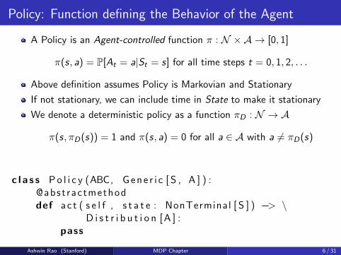
Policy: Function defining the Behavior of the Agent

A Policy is an Agent-controlled function π : N ×A → [0, 1]

π(s, a) = P[At = a|St = s] for all time steps t = 0, 1, 2, . . .

Above definition assumes Policy is Markovian and Stationary

If not stationary, we can include time in State to make it stationary

We denote a deterministic policy as a function πD : N → A

π(s, πD(s)) = 1 and π(s, a) = 0 for all a ∈ A with a 6= πD(s)

c l a s s P o l i c y (ABC, G e n e r i c [ S , A ] ) :@abst ractmethoddef a c t ( s e l f , s t a t e : NonTerminal [ S ] ) −> \

D i s t r i b u t i o n [ A ] :pass


[MDP, Policy] := MRP

PπR(s, r , s ′) =∑a∈A

π(s, a) · PR(s, a, r , s ′)

Pπ(s, s ′) =∑a∈A

π(s, a) · P(s, a, s ′)

RπT (s, s ′) =∑a∈A

π(s, a) · RT (s, a, s ′)

Rπ(s) =∑a∈A

π(s, a) · R(s, a)


@abstractclass MarkovDecisionProcess

c l a s s M a r k o v D e c i s i o n P r o c e s s (ABC, G e n e r i c [ S , A ] ) :@abst ractmethoddef a c t i o n s ( s e l f , s t a t e : NonTerminal [ S ] ) \

−> I t e r a b l e [ A ] :pass

@abst ractmethoddef s t e p ( s e l f , s t a t e : NonTerminal [ S ] , a c t i o n : A) \

−> D i s t r i b u t i o n [ Tuple [ S t a t e [ S ] , f l o a t ] ] :pass


@abstractclass MarkovDecisionProcess

def a p p l y p o l i c y ( s e l f , p o l i c y : P o l i c y [ S , A ] ) \−> MarkovRewardProcess [ S ] :

mdp = s e l f

c l a s s RewardProcess ( MarkovRewardProcess [ S ] ) :def t r a n s i t i o n r e w a r d (

s e l f ,s t : NonTerminal [ S ]

) −> D i s t r i b u t i o n [ Tuple [ S t a t e [ S ] , f l o a t ] ] :a c t i o n s : D i s t r i b u t i o n [ A ] = p o l i c y . a c t ( s t )return a c t i o n s . apply (

lambda a : mdp . s t e p ( st , a ))

return RewardProcess ( )


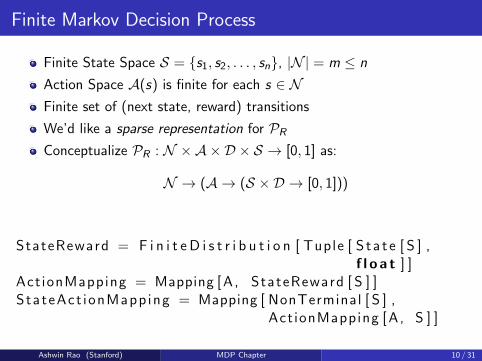
Finite Markov Decision Process

Finite State Space S = {s1, s2, . . . , sn}, |N | = m ≤ n

Action Space A(s) is finite for each s ∈ NFinite set of (next state, reward) transitions

We’d like a sparse representation for PRConceptualize PR : N ×A×D × S → [0, 1] as:

N → (A → (S × D → [0, 1]))

StateReward = F i n i t e D i s t r i b u t i o n [ Tuple [ S t a t e [ S ] ,f l o a t ] ]

Act ionMapping = Mapping [ A, StateReward [ S ] ]StateAct ionMapp ing = Mapping [ NonTerminal [ S ] ,

Act ionMapping [ A, S ] ]


class FiniteMarkovDecisionProcess

c l a s s F i n i t e M a r k o v D e c i s i o n P r o c e s s (M a r k o v D e c i s i o n P r o c e s s [ S , A ]

) :m: StateAct ionMapp ing [ S , A ]n t s t a t e s : Sequence [ NonTerminal [ S ] ]

def i n i t ( s e l f , m: Mapping [ S , Mapping [ A,F i n i t e D i s t r i b u t i o n [ Tuple [ S , f l o a t ] ] ] ] ) :

nt : Set [ S ] = set ( mapping . k e y s ( ) )s e l f .m = {NonTerminal ( s ) : {a : C a t e g o r i c a l (

{( NonTerminal ( s1 ) i f s1 i n nt e l s eTermina l ( s1 ) , r ) : p f o r ( s1 , r ) , p i nv . t a b l e ( ) . i t e m s ( )} ) f o r a , v i nd . i t e m s ( )} f o r s , d i n mapping . i t e m s ( )}

s e l f . n t s t a t e s = l i s t ( s e l f .m. k e y s ( ) )


class FinitePolicy

def s t e p ( s e l f , s t a t e : NonTerminal [ S ] , a c t i o n : A) \−> StateReward :

return s e l f . mapping [ s t a t e ] [ a c t i o n ]

@ d a t a c l a s s ( f r o z e n=True )c l a s s F i n i t e P o l i c y ( P o l i c y [ S , A ] ) :

p o l i c y m a p : Mapping [ S , F i n i t e D i s t r i b u t i o n [ A ] ]

def a c t ( s e l f , s t a t e : NonTerminal [ S ] ) \−> F i n i t e D i s t r i b u t i o n [ A ] :

return s e l f . p o l i c y m a p [ s t a t e . s t a t e ]

With this, we can write a method for FiniteMarkovDecisionProcess thattakes a FinitePolicy and produces a FiniteMarkovRewardProcess


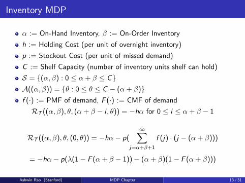
Inventory MDP

α := On-Hand Inventory, β := On-Order Inventory

h := Holding Cost (per unit of overnight inventory)

p := Stockout Cost (per unit of missed demand)

C := Shelf Capacity (number of inventory units shelf can hold)

S = {(α, β) : 0 ≤ α + β ≤ C}A((α, β)) = {θ : 0 ≤ θ ≤ C − (α + β)}f (·) := PMF of demand, F (·) := CMF of demand

RT ((α, β), θ, (α + β − i , θ)) = −hα for 0 ≤ i ≤ α + β − 1

RT ((α, β), θ, (0, θ)) = −hα− p(∞∑

j=α+β+1

f (j) · (j − (α + β)))

= −hα− p(λ(1− F (α + β − 1))− (α + β)(1− F (α + β)))


State-Value Function of an MDP for a Fixed Policy

Define the Return Gt from state St as:

Gt =∞∑

i=t+1

γ i−t−1 · Ri = Rt+1 + γ · Rt+2 + γ2 · Rt+3 + . . .

γ ∈ [0, 1] is the discount factor

State-Value Function (for policy π) V π : N → R defined as:

V π(s) = Eπ,PR[Gt |St = s] for all s ∈ N , for all t = 0, 1, 2, . . .

V π is Value Function of π-implied MRP, satisfying MRP Bellman Eqn

V π(s) = Rπ(s) + γ ·∑s′∈N

Pπ(s, s ′) · V π(s ′)

This yields the MDP (State-Value Function) Bellman Policy Equation

V π(s) =∑a∈A

π(s, a) · (R(s, a) + γ ·∑s′∈N

P(s, a, s ′) · V π(s ′)) (1)


Action-Value Function of an MDP for a Fixed Policy

Action-Value Function (for policy π) Qπ : N ×A → R defined as:

Qπ(s, a) = Eπ,PR[Gt |(St = s,At = a)] for all s ∈ N , a ∈ A

V π(s) =∑a∈A

π(s, a) · Qπ(s, a) (2)

Combining Equation (1) and Equation (2) yields:

Qπ(s, a) = R(s, a) + γ ·∑s′∈N

P(s, a, s ′) · V π(s ′) (3)

Combining Equation (3) and Equation (2) yields:

Qπ(s, a) = R(s, a) + γ ·∑s′∈N

P(s, a, s ′)∑a′∈A

π(s ′, a′) · Qπ(s ′, a′) (4)

MDP Prediction Problem: Evaluating V π(·) and Qπ(·) for fixed policy πAshwin Rao (Stanford) MDP Chapter 15 / 31

MDP State-Value Function Bellman Policy Equation


MDP Action-Value Function Bellman Policy Equation


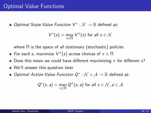
Optimal Value Functions

Optimal State-Value Function V ∗ : N → R defined as:

V ∗(s) = maxπ∈Π

V π(s) for all s ∈ N

where Π is the space of all stationary (stochastic) policies

For each s, maximize V π(s) across choices of π ∈ Π

Does this mean we could have different maximizing π for different s?

We’ll answer this question later

Optimal Action-Value Function Q∗ : N ×A → R defined as:

Q∗(s, a) = maxπ∈Π

Qπ(s, a) for all s ∈ N , a ∈ A


Bellman Optimality Equations

V ∗(s) = maxa∈A

Q∗(s, a) (5)

Q∗(s, a) = R(s, a) + γ ·∑s′∈N

P(s, a, s ′) · V ∗(s ′) (6)

These yield the MDP State-Value Function Bellman Optimality Equation

V ∗(s) = maxa∈A{R(s, a) + γ ·

∑s′∈N

P(s, a, s ′) · V ∗(s ′)} (7)

and the MDP Action-Value Function Bellman Optimality Equation

Q∗(s, a) = R(s, a) + γ ·∑s′∈N

P(s, a, s ′) ·maxa′∈A

Q∗(s ′, a′) (8)

MDP Control Problem: Computing V ∗(·) and Q∗(·)


MDP State-Value Function Bellman Optimality Equation


MDP Action-Value Function Bellman Optimality Equation


Optimal Policy

Bellman Optimality Equations don’t directly solve Control

Because (unlike Bellman Policy Equations), these are non-linear

But these equations form the foundations of DP/RL algos for Control

But will solving Control give us the Optimal Policy?

What does Optimal Policy mean anyway?

What if different π maximize V π(s) for different s?

So define an Optimal Policy π∗ as one that ”dominates” all other π:

π∗ ∈ Π is an Optimal Policy if V π∗(s) ≥ V π(s) for all π and for all s

Is there an Optimal Policy π∗ such that V ∗(s) = V π∗(s) for all s?


Optimal Policy achieves Optimal Value Function

Theorem

For any (discrete-time, countable-spaces, time-homogeneous) MDP:

There exists an Optimal Policy π∗ ∈ Π, i.e., there exists a Policyπ∗ ∈ Π such thatV π∗(s) ≥ V π(s) for all policies π ∈ Π and for all states s ∈ NAll Optimal Policies achieve the Optimal Value Function, i.e.V π∗(s) = V ∗(s) for all s ∈ N , for all Optimal Policies π∗

All Optimal Policies achieve the Optimal Action-Value Function, i.e.Qπ∗(s, a) = Q∗(s, a) for all s ∈ N , for all a ∈ A, for all OptimalPolicies π∗


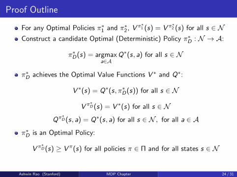
Proof Outline

For any Optimal Policies π∗1 and π∗2, V π∗1 (s) = V π∗2 (s) for all s ∈ NConstruct a candidate Optimal (Deterministic) Policy π∗D : N → A:

π∗D(s) = argmaxa∈A

Q∗(s, a) for all s ∈ N

π∗D achieves the Optimal Value Functions V ∗ and Q∗:

V ∗(s) = Q∗(s, π∗D(s)) for all s ∈ N

V π∗D (s) = V ∗(s) for all s ∈ N

Qπ∗D (s, a) = Q∗(s, a) for all s ∈ N , for all a ∈ A

π∗D is an Optimal Policy:

V π∗D (s) ≥ V π(s) for all policies π ∈ Π and for all states s ∈ N


State Space Size and Transitions Complexity

Tabular Algorithms for State Spaces that are not too large

In real-world, state spaces are very large/infinite/continuous

Curse of Dimensionality: Size Explosion as a function of dimensions

Curse of Modeling: Transition Probabilities hard to model/estimate

Dimension-Reduction techniques, Unsupervised ML methods

Function Approximation of the Value Function (in ADP and RL)

Sampling, Sampling, Sampling ... (in ADP and RL)


Action Space Sizes

Large Action Spaces: Hard to represent, estimate and evaluate:

Policy πAction-Value Function for a policy Qπ

Optimal Action-Value Function Q∗

Large Actions Space makes it hard to calculate argmaxa Q(s, a)

Optimization over Action Space for each non-terminal state

Policy Gradient a technique to deal with large action spaces


Time-Steps Variants and Continuity

Time-Steps: terminating (episodic) or non-terminating (continuing)

Discounted or Undiscounted MDPs, Average-Reward MDPs

Continuous-time MDPs: Stochastic Processes and Stochastic Calculus

When States/Actions/Time all continuous, Hamilton-Jacobi-Bellman


Partially-Observable Markov Decision Process (POMDP)

Two different notions of State:

Internal representation of the environment at each time step t (S(e)t )

The agent’s state at each time step t (let’s call it S(a)t )

We assumed S(e)t = S

(a)t (= St) and that St is fully observable

A more general framework assumes agent sees Observations Ot

Agent cannot see (or infer) S(e)t from history of observations

This more general framework is called POMDP

POMDP is specified with Observation Space O and observationprobability function Z : S ×A×O → [0, 1] defined as:

Z(s ′, a, o) = P[Ot+1 = o|(St+1 = s ′,At = a)]

Along with the usual transition probabilities specification PRMDP is a special case of POMDP with Ot = S

(e)t = S

(a)t = St


POMDP Framework


Belief States, Tractability and Modeling

Agent doesn’t have knowledge of St , only of Ot

So Agent has to “guess” St by maintaining Belief States

b(h)t = (P[St = s1|Ht = h],P[St = s2|Ht = h], . . .)

where history Ht is all data known to agent by time t:

Ht := (O0,R0,A0,O1,R1,A1, . . . ,Ot ,Rt)

Ht satisfies Markov Property ⇒ b(h)t satisfies Markov Property

POMDP yields (huge) MDP whose states are POMDP’s belief states

Real-world: Model as accurate POMDP or approx as tractable MDP?


Key Takeaways from this Chapter

MDP Bellman Policy Equations

MDP Bellman Optimality Equations

Existence of an Optimal Policy, and of each Optimal Policy achievingthe Optimal Value Function


a guided tour of chapter 2: markov decision process and

Documents