a ghost-cell immersed boundary method for flow in complex geometry

www.elsevier.com/locate/jcp

Journal of Computational Physics 192 (2003) 593–623

A ghost-cell immersed boundary method for flowin complex geometry

Yu-Heng Tseng *, Joel H. Ferziger

Environmental Fluid Mechanics Laboratory, Stanford University, Stanford, CA 94305-4020, USA

Received 9 September 2002; received in revised form 26 May 2003; accepted 31 July 2003

Abstract

An efficient ghost-cell immersed boundary method (GCIBM) for simulating turbulent flows in complex geometries is

presented. A boundary condition is enforced through a ghost cell method. The reconstruction procedure allows sys-

tematic development of numerical schemes for treating the immersed boundary while preserving the overall second-

order accuracy of the base solver. Both Dirichlet and Neumann boundary conditions can be treated. The current ghost

cell treatment is both suitable for staggered and non-staggered Cartesian grids. The accuracy of the current method is

validated using flow past a circular cylinder and large eddy simulation of turbulent flow over a wavy surface. Numerical

results are compared with experimental data and boundary-fitted grid results. The method is further extended to an

existing ocean model (MITGCM) to simulate geophysical flow over a three-dimensional bump. The method is easily

implemented as evidenced by our use of several existing codes.

� 2003 Elsevier B.V. All rights reserved.

1. Introduction

In computational fluid dynamics, including geophysical fluid dynamics (GFD), the primary issues are

accuracy, computational efficiency, and, especially, the handling of complex geometry. All large-scale

geophysical flows involve complex three-dimensional geometry and turbulence. Accurate representation ofmulti-scale, time-dependent physical phenomena is required. A grid that is not well suited to the problem

can lead to unsatisfactory results, instability, or lack of convergence.

The development of accurate and efficient methods that can deal with arbitrarily complex geometry

would represent a significant advance. The immersed boundary method (IBM) has recently been demon-

strated to be applicable to complex geometries while requiring significantly less computation than com-

peting methods without sacrificing accuracy [8,44]. The IBM specifies a body force in such a way as to

simulate the presence of a surface without altering the computational grid. The main advantages of the

*Corresponding author. Tel.: +1-650-725-5948; fax: +1-650-725-3525.

E-mail address: [email protected] (Y.-H. Tseng).

0021-9991/$ - see front matter � 2003 Elsevier B.V. All rights reserved.

doi:10.1016/j.jcp.2003.07.024

mail to: [email protected]

594 Y.-H. Tseng, J.H. Ferziger / Journal of Computational Physics 192 (2003) 593–623

IBM are memory and CPU savings and ease of grid generation compared to unstructured grid methods

[44]. Bodies of almost arbitrary shape can be dealt with. Furthermore, flows with multiple bodies or islands

may be computed at reasonable computational cost.The IBM was first introduced by Peskin [36]. More recently, Goldstein et al. [15] and Saiki and Biringen

[38] published extensions. They employed feedback forcing to represent the effect of solid body. The

feedback force is added to the momentum equation to bring the fluid velocity to zero at the desired points.

However, this technique may induce spurious oscillations and restricts the computational time step [15],

effectively limiting the technique to two-dimensions. Mohd-Yusof [33] suggested an approach that intro-

duces a body-force f such that the desired velocity distribution V is obtained at the boundary X. Inprinciple, there are no restrictions on the velocity distribution V or the motion of X. He implemented the

method for a complex geometry in a pseudo-spectral code while avoiding the need of a small computationaltime step. The method costs no more than the base computational scheme. Fadlun et al. [8] applied this

approach to a three-dimensional finite-difference method on a staggered grid and showed that the approach

was more efficient than feedback forcing.

A number of other immersed boundary methods have been applied to problems of irregular geometry.

Calhoun and LeVeque [3,4] proposed a streamfunction-vorticity method to model irregular shapes in a

Cartesian grid. The irregular boundary is represented by discontinuity conditions. They extended the

method developed by McKenney et al. [32] to solve a Poisson equation on an irregular region using a

Cartesian grid. Pember et al. [35] presented an adaptive Cartesian mesh solver for the Euler equations.Their method treats the boundary cells as regular cells, thus avoiding instability problems. Almgren et al. [2]

developed a Cartesian grid projection method for the incompressible Euler equations in complex geometry.

The same group also proposed a second-order accurate method for solving the Poisson equation on two-

dimensional Cartesian grids with embedded boundaries [21]. McCorquodale et al. [31] extended this ap-

proach to the solution of the time-dependent heat equation. On the other hand, Udaykumar et al. [42] and

Ye et al. [46] have presented a finite-volume Cartesian method without momentum forcing. They reshaped

the immersed boundary cells to fit the local geometry and used quadratic interpolation to calculate the

fluxes across the cell faces while preserving second-order accuracy. They showed that the method is ap-plicable to moving geometry problems. However, the above studies mainly focus on two-dimensional

applications. Particularly, the streamfunction-vorticity method is hard to extend to three dimensions.

Kirkpatrick et al. [24] present a second-order accurate IBM on a non-uniform, staggered three-dimensional

Cartesian grid. The approach requires truncating the Cartesian cells at the boundary to create new three-

dimensional cells which conform to the shape of the surface. The reshaped-cell method developed by

Kirkpatrick et al. [24], Udaykumar et al. [42], and Ye et al. [46] is very similar to the shaved cell approach in

MIT General Ocean Model (MITGCM) [1]. However, the implementation for the reshaped cell approach is

complicated and only no-slip boundary conditions can be applied. Kim et al. [22] developed an immersedboundary method that uses both momentum forcing and mass sources/sinks. An extensive review of the

immersed boundary methods for turbulent flow simulations can be found in [19].

In this paper, we extend the idea of Fadlun et al. [8] and Verzicco et al. [43] via a ghost cell approach. In

Fadlun et al. [8], the velocity at the first grid point outside the body (ui in Fig. 1) is obtained by linearly

interpolating the velocity at the second grid point (uiþ1) and the velocity at the body surface (V ), see Fig. 1.This approach applies momentum forcing within the flow field. The interpolation direction (the direction to

the second grid point) used by Fadlun et al. [8] is either the streamwise (x) or the transverse (y) direction.

They also successfully implemented the immersed boundary algorithm in large-eddy simulation (LES) ofturbulent flow in a motored axisymmetric piston-cylinder assembly [44]. This approach does not reduce the

stability of the underlying time-integration scheme and very good quantitative agreement with experimental

measurements was obtained. For comparable accuracy, the computational requirements for the IBM ap-

proach are much lower than simulations on an unstructured, boundary-fitted mesh as given in previous

published paper [17,44].

Fig. 1. Sketch of the velocity interpolation procedure in [8].

Y.-H. Tseng, J.H. Ferziger / Journal of Computational Physics 192 (2003) 593–623 595

The current approach attempts to achieve higher-order representation of the boundary using a ghost

zone inside the body. The ghost cell method is very popular for treating two-phase flows, obtaining accurate

discretization across the interface [9,10,45]. The particular method proposed by Fedkiw et al. [9,10] isknown as the Ghost Fluid Method (GFM) and was developed to capture discontinuities such as shocks,

detonations and deflagrations. They also used the technique to solve a variable coefficient Poisson equation

on an irregular domain using a Cartesian grid [14,28]. Forrer and Jeltsch [12] provided a higher-order wall

treatment based on Cartesian grids using the ghost-cell idea. However, the method has been implemented

only for two-dimensional compressible inviscid flows with symmetry boundary conditions. In GFD, the

ghost cell method promises to not only represent realistic complex geometry but also provide the flexibility

needed to impose various boundary conditions including a log-law boundary condition.

We describe the systematic treatment of various boundary conditions in Section 2. The approach im-poses the specified boundary condition by extrapolating the variable to a ghost node inside the body. High-

order extrapolation is used to preserve the overall accuracy. The present approach is more flexible with

respect to the incorporation of boundary conditions. In order to verify the accuracy of the IBM, flow over a

circular cylinder and a three-dimensional turbulent flow over wavy boundary are simulated using LES.

Both results are compared with published experiments and boundary-fitted grid simulations. We also ex-

tend the current approach to an existing ocean model and compared the IBM results with previous stair-

step and partial-cell ones. The main advantage of the current approach is the ease of programming, which

requires only that an immersed boundary module be added to an existing code.The current method can readily be implemented in any existing Cartesian grid code. This paper is or-

ganized as follows. Section 2 introduces the governing equations and numerical implementation of the

method. The generalized ghost cell method and the polynomial reconstruction schemes are laid out. Dif-

ferent boundary conditions and the implementation to both non-staggered and staggered grids are dis-

cussed. Section 3 validates the approach for flow over a cylinder and evaluates the accuracy. We also extend

the new method to LES of three-dimensional turbulent flow over wavy boundary using a Cartesian grid and

compares the results with a well-resolved boundary-fitted grid simulation. Section 4 illustrates the imple-

mentation to MIT global circulation model (MITGCM) and compares with previous methods for a geo-physical flow. Finally, conclusions are drawn in Section 5.


2. Numerical methods

2.1. Governing equations

The objective of our study is to develop an efficient flow solver using the IBM. In most stratified flows,

the density varies by only a few percent so we may employ the Boussinesq approximation. The governing

equations express mass and momentum conservation. A boundary forcing term fi is added to the mo-

mentum equation

oujoxj

¼ 0; ð1Þ

ouiot

þ oFijoxj

¼ fi; ð2Þ

where the flux is

Fij ¼ uiuj þ Pdij � mouioxj

�þ ouj

oxi

�: ð3Þ

Here, P is the pressure divided by the fluid density q, m ¼ l=q0 is the kinematic viscosity, and repeated

indices imply summation. The boundary forcing fi is imposed implicitly through a ghost-cell method de-scribed below and is only active at the boundary.

2.2. Ghost cell immersed boundary method (GCIBM)

The treatment of the momentum equation is now defined at each time step so as to enforce the boundary

condition, thus the approach is similar to the forcing used by Mohd-Yusof [33] and Fadlun et al. [8]. The

force depends on the location and the fluid velocity and thus is a function of time. Its location, xi is notgenerally coincident with the grid but the forcing must be extrapolated to these nodes. The forcing fi is zeroinside the fluid and is non-zero in the ghost cell zone which is used to represent the presence of complex

boundary. If the Navier–Stokes (N–S) equation (2) is discretized as

unþ1i � uniDt

¼ RHSi þ fi; ð4Þ

where RHSi contains convective and viscous terms and the pressure gradient. The boundary conditions can

be either Dirichlet or Neumann types.

The current ghost cell method extrapolates the velocity (V nþ1i ) and pressure fields to the ghost cells using

nearby fluid points and associated boundary information (see Section 2.3). As an example, if the forcing fimust yield unþ1

i ¼ V nþ1i in accord with the immersed boundary condition, we obtain

fi ¼ �RHSi þV nþ1 � un

Dt: ð5Þ

This forcing causes the desired boundary condition to be satisfied at every time step. There are no free

constants and the boundary conditions are enforced to within the numerical precision. Evaluating the force

fi requires essentially no additional CPU time since there are no new terms to compute. Nor does it

influence the stability of the time advancement scheme.


The force in Eq. (5) is correct for the case in which the position of the unknowns on the grid coincides

with the immersed boundary; this requires the boundary to lay on coordinate lines or surfaces, which is not

possible for complex geometries. Many different techniques have been adopted and they can be classifiedinto two groups: (a) schemes that spread the forcing function over the vicinity of the immersed surface and

(b) schemes that produce a local reconstruction of the solution based on the boundary values [19]. In fact,

the two approaches are equivalent. The original Peskin [36] method, which substitutes a discrete Dirac dfunction in Eq. (5), belongs to the first category. The local reconstruction scheme (b) has been proven to be

more flexible [8,44] and can be designed so that it has high degree of accuracy. The current ghost cell

method belongs to the second category. The numerical procedure we use is the following:

1. Detect the boundary and determine the adjacent ghost cells (preliminary step).

2. Extrapolate to find the ghost cell value required to impose the boundary condition implicitly. Theinterpolation scheme is discussed in Sections 2.3 and 2.4.

3. Obtain the predicted field (intermediate velocity u�i ) of the fractional step procedure [11,23].

4. Solve the pressure Poisson equation to satisfy the continuity equation. Some discussion of the pressure

solver is provided in Section 3.2.

5. Update the velocity field (unþ1i ) to the next time step.

The immersed boundary is represented by piecewise linear segments. We identify the cells that are cut by

the boundary and determine the intersections of the immersed boundary with the sides of these cells. The

computational domain is divided into two regions: the physical domain and the ghost cell domain. They areillustrated in Fig. 2(a). The physical domain is the flow region (x). The ghost cells lie just inside the body

adjacent to computational nodes in the flow domain. The values of flow variables at the ghost cells are

computed using a local reconstruction scheme involving the ghost node and neighboring flow nodes.

The ghost cells can be detected automatically if a structured domain is used. All of the possibilities for

the boundary line intersecting an arbitrary cell are shown in Fig. 3. Each node is the center of a rectangular

cell and x is the cell center. A cell belongs to the physical flow domain if the immersed boundary does not

cover the cell center as in Figs. 3(a) and (c). The shaded areas are inside the boundary. If the immersed

Fig. 2. (a) Schematic of computational domain with an immersed boundary. x, point in the physical domain and n, the ghost cell

domain. (b) Schematic of the points used to evaluate the variable located at a ghost cell G point.

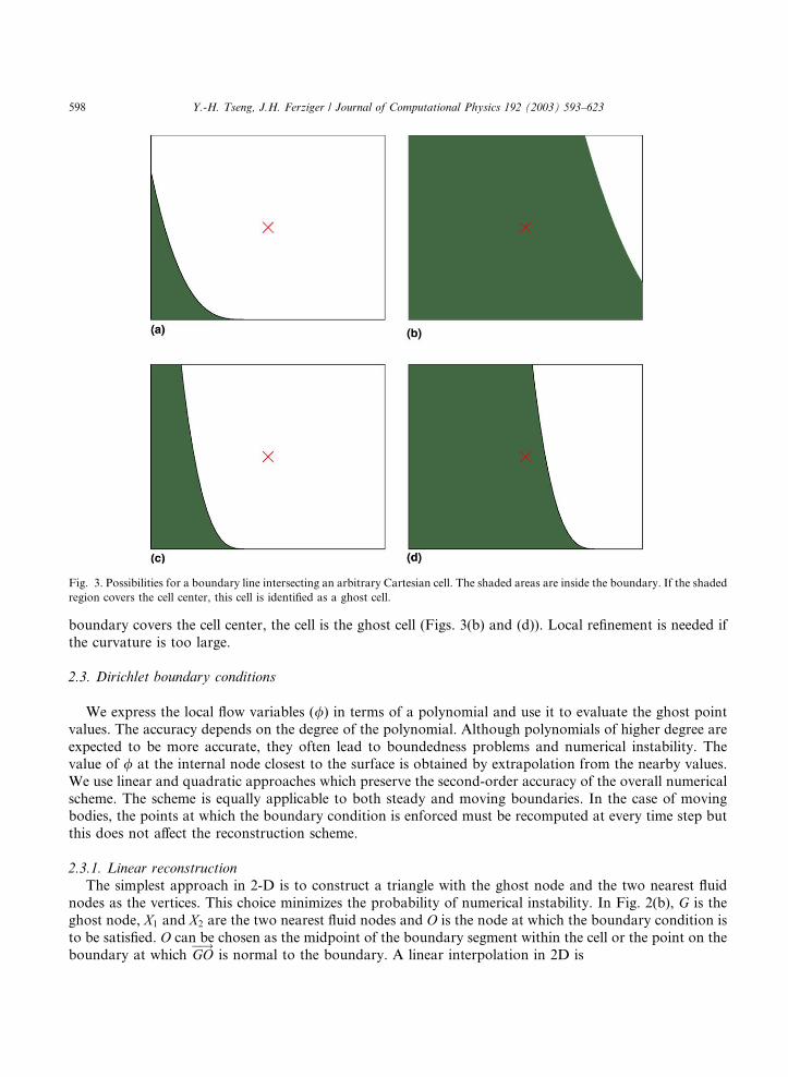
Fig. 3. Possibilities for a boundary line intersecting an arbitrary Cartesian cell. The shaded areas are inside the boundary. If the shaded

region covers the cell center, this cell is identified as a ghost cell.


boundary covers the cell center, the cell is the ghost cell (Figs. 3(b) and (d)). Local refinement is needed if

the curvature is too large.

2.3. Dirichlet boundary conditions

We express the local flow variables (/) in terms of a polynomial and use it to evaluate the ghost point

values. The accuracy depends on the degree of the polynomial. Although polynomials of higher degree are

expected to be more accurate, they often lead to boundedness problems and numerical instability. The

value of / at the internal node closest to the surface is obtained by extrapolation from the nearby values.

We use linear and quadratic approaches which preserve the second-order accuracy of the overall numerical

scheme. The scheme is equally applicable to both steady and moving boundaries. In the case of movingbodies, the points at which the boundary condition is enforced must be recomputed at every time step but

this does not affect the reconstruction scheme.

2.3.1. Linear reconstruction

The simplest approach in 2-D is to construct a triangle with the ghost node and the two nearest fluid

nodes as the vertices. This choice minimizes the probability of numerical instability. In Fig. 2(b), G is the

ghost node, X1 and X2 are the two nearest fluid nodes and O is the node at which the boundary condition is

to be satisfied. O can be chosen as the midpoint of the boundary segment within the cell or the point on the

boundary at which GO�!

is normal to the boundary. A linear interpolation in 2D is


/ ¼ a0 þ a1xþ a2y: ð6Þ

The ghost cell value is a weighted combination of the values at the nodes (X1, X2 and O). The coefficients canbe expressed in terms of the nodal values

a ¼ B�1/; ð7Þ

where, for linear interpolation, B is a 3� 3 matrix whose elements can be computed from the coordinates of

the three points. When the velocity at the boundary is specified,

B ¼1 x0 y01 x1 y11 x2 y2

24

35: ð8Þ

It is convenient to evaluate the matrices B at each point initially and store them for use during the

solution procedure. The major drawback with this extrapolation is that large negative weighting coefficients

are encountered when the boundary point is close to one of the fluid nodes used in the extrapolation.

Although algebraically correct, this can lead to numerical instability, i.e., the absolute value at the ghost

point may be greater than the nearby fluid point values and the solution may not converge.Two approaches are used to remedy the difficulty. The first is to use the image of the ghost node inside

the flow domain [29] to ensure positive weighting coefficients. The point I is the image of the ghost node Gthrough the boundary as shown in Fig. 4(a). The flow variable is evaluated at the image point using the

interpolation scheme. The value at the ghost node is then /G ¼ 2/O � /I .

The other approach is to alter the piecewise linear boundary. When the boundary is close to a fluid node

(normal distance of fluid point G0 to the boundary OG0 < 0:1Dx, Dx is the cell size) and far from the ghost

point as in Fig. 4(b), we simply move the boundary point to the fluid node closest to the boundary [14].

Since the boundary is approximated as piecewise linear, the accuracy is hardly affected when the boundarysegment is divided into two pieces, see Fig. 4(b). Gibou et al. [14] demonstrated that this approach could be

used to obtain the second order accuracy in solving Poisson equation on irregular domain. The original

piecewise linear boundary is shown as the dash-dot (–�) line connecting boundary intercepts. This ensures

Fig. 4. Special treatment to minimize numerical instability. (a) Schematic of a ghost cell using the image method (I is the image point).

(b) Schematic of adding an additional ghost cell G0 if the boundary is close to the fluid points. –� is the linear piecewise approximation

to the boundary. � � � is the boundary approximated by two piecewise segments.


that large negative weighting coefficients will not occur. The following numerical example adopts the first

approach since additional image point is involved.

2.3.2. Quadratic reconstruction

Most second-order accurate finite volume flow solvers assume quadratic variation of flow variables near

the wall. Use of higher-order interpolation retains the formal second-order accuracy of the scheme. In twodimensions, if the flow variables are assumed to vary in a quadratic manner in both the x and y directions,

the value of / is expressed as

/ ¼ a0 þ a1xþ a2y þ a3x2 þ a4xy þ a5y2: ð9Þ

The six constants of the assumed polynomial are evaluated from five neighboring fluid nodes and thewall point (Fig. 2(b)). The matrix B in Eq. (7) is replaced by a 6� 6 matrix

B ¼1 x0 y0 x20 x0y0 y201 x1 y1 x21 x1y1 y21� � � � � � � � � � � � � � � � � �1 x5 y5 x25 x5y5 y25

2664

3775: ð10Þ

The ghost node values are either extrapolated or evaluated using an image point. The reconstruction

procedure is similar to that for the linear polynomial. The influence of the schemes on the overall accuracy

is compared in the numerical examples. Majumdar et al. [29] tested the ghost-cell immersed boundary using

second-order bilinear and quadratic interpolation schemes for a RANS solver and they found that the

solutions do not have any significant difference.

For three-dimensional domains, we need to modify the interpolation scheme in Eqs. (6) and (9). More

neighbor nodes are involved, e.g., for linear reconstruction, the variable in the cell center is interpolated

using four points (three nearest neighbor nodes and one boundary point are involved). A three-dimensionalillustration is shown in Fig. 5. The black dots (d) represent the three closest neighboring cells with respect

to the boundary point O, see Fig. 5. These points can be located initially and stored. For quadratic

Fig. 5. Schematic of the points used to evaluate the variable located at a ghost cell point G in three dimension. Linear construction

relies on three nearest neighbor nodes and a boundary surface point (point O).


reconstruction, 10 points (nine neighbors) are needed. The remainder of the solution procedure remains the

same as that described above. A 4� 4 linear system will be solved for linear construction and a 10� 10

system will be solved for quadratic one.Furthermore, more elaborate, high-order schemes may be used in three dimensions. It is well known that

high-order polynomial interpolations may introduce wiggles and spurious extrema. The inverse distance

weighting proposed by Franke [13] has the property of preserving local maxima and producing smooth

reconstruction. This scheme is suitable for reconstructing variables that are smoothly varying without

exhibiting large maxima. The interpolation at the ghost cell is

/G ¼Xn

m¼1

wm/m=q; ð11Þ

wm ¼ R� hmRhm

� �p

; ð12Þ

q ¼Xn

l¼1

R� hlRhl

� �p

; ð13Þ

where /m (/G) represents the solution at a certain location (ghost cell), wm represents the weight and hm isthe distance between the ghost cell (/G) and the location of /m. p is an arbitrary positive real number called

the power parameter (typically p ¼ 2). R is the distance from the ghost point to the most distant point used

in the construction and n is the total number of the construction points.

It is important to note that for the forcing of Saiki and Biringen [38] and Goldstein et al. [15], the velocity

at the immersed boundaries was imposed by the fictitious force. In the current approach, the boundary

condition is imposed directly. This implies that, in contrast to the feedback forcing method, the stability

limit of the current integration scheme is the same as that without the immersed boundaries, thus making

simulation of complex three-dimensional flows practical. Higher-order extrapolation/interpolation schemesto evaluate the variables at the ghost cells can preserve at least second-order spatial accuracy [42,46].

2.4. Neumann boundary conditions

The method computes the velocity up to the boundary using the neighboring points. With the poly-

nomial reconstruction scheme, we do not solve any equations on the ghost cells. The treatment of Dirichlet

boundary conditions has been described in the non-staggered Cartesian grid approach. A similar scheme

can be used for Neumann boundary conditions. The only difference is in the construction of matrix B in Eq.

(7). This makes the current approach applicable to a variety of boundary conditions.

For example, the pressure boundary condition requires the wall normal derivative to be zero at the

boundary

oPon

��X

¼ 0: ð14Þ

The normal derivative on the boundary can be decomposed as

oPon

¼ oPox

n̂nx þoPoy

n̂ny ; ð15Þ

where n̂nx and n̂ny are the components of the unit vector normal to the boundary. Since n̂nx and n̂ny are known,the computation of the normal gradient at any point is straightforward. Linear reconstruction requires two


fluid nodes and one boundary node. The Neumann condition at the boundary node is stored in the first

element of / in Eq. (7) and the known flow variables on the two fluid nodes are stored in the second and

third elements of /. Quadratic reconstruction requires five fluid nodes and one boundary node. See Fig. 2(b)

for the notation. Index O locates the boundary, tanðh0Þ is the slope of the normal at the surface O.(a) Linear reconstruction

B ¼0 � sinðh0Þ cosðh0Þ1 x1 y11 x2 y2

24

35;

where h0 is the local slope at the boundary node.

(b) Quadratic reconstruction

B ¼

0 � sinðh0Þ cosðh0Þ �2 sinðh0Þx0 cosðh0Þx0 � sinðh0Þy0 2 cosðh0Þy01 x1 y1 x21 x1y1 y21� � � � � � � � � � � � � � � � � �1 x5 y5 x25 x5y5 y25

2664

3775:

Finally, the coefficients can be obtained systematically for both reconstructions:

a0a1� � �am

2664

3775 ¼ B�1

oP0onP1� � �Pm

2664

3775; ð16Þ

where index m is 2 for linear reconstruction (three unknowns) and is 5 for quadratic reconstruction (six

unknowns). oP0=on is the Neumann boundary condition for pressure and Pm is the neighboring pressure

field. The flexibility of current approach is demonstrated by the examples presented in Section 3.

2.5. Mixed Dirichlet and Neumann types (Robin boundary condition)

Sometimes, one has a mixed or Robin boundary condition in a physical/engineering problem. A linear

combination of the variable (/) and its wall normal derivative is prescribed.

a/þ bo/on

¼ f ; ð17Þ

where f is the known function which specifies the boundary value, a and b are the linear combination

coefficients. Since our ghost cell method solves a linear system (Eq. (7)) at each boundary grid point, the

ghost cell variables for the mixed Robin boundary can be expressed by solving the following system for

interpolation coefficients aR:

aR ¼ B�1R /; ð18Þ

where BR ¼ aBD þ bBN is a linear combination of the matrices BD and BN, the matrices for Dirichlet and

Neumann conditions. a and b are the coefficients from the Robin boundary condition. In general, the

current ghost cell approach is flexible in the choice of boundary condition and imposes a forcing function

implicitly through the ghost cell.


2.6. Non-staggered and staggered grid arrangements

The above immersed boundary treatment focuses on the non-staggered (collocated) grid arrangement.

Whether a cell is a ghost cell or not is determined by the relation between the cell center and the physical

boundary. The use of staggered grids for the solution of the N–S equations has a number of advantages.Fadlun et al. [8] applied the IBM approach to a three-dimensional finite-difference method on a staggered

grid. However, they did not use ghost cells and their interpolation scheme is applied only in the x or ydirections. The current ghost-cell approach can be easily extended to staggered grid arrangement in which

all three velocity components and the pressure are computed on different grids. For each velocity com-

ponent and pressure, we can find different weighted coefficients at the boundary, i.e., we need to solve a

different linear system for each variable. A numerical example of a staggered grid treatment is given in

Section 4. A two-dimensional schematic of the velocity allocation is shown in Fig. 6. The U and V

components are located on different faces for each cell. The staggered grid arrangement increases therequired storage. However, the increase is not significant since the boundary is lower dimensional than the

domain.

2.7. Summary

The generalized GCIBM and the polynomial reconstruction schemes are laid out for various boundary

conditions. It is worth pointing out how our methodology differs from the immersed boundary method of

Ye et al. [46] and Fadlun et al. [8]. First, the interpolation scheme differs from theirs. Second, the reshaped

cell method in [46] complicates the numerical algorithm and extension to other boundary conditions and

moving boundaries is difficult. Third, the current approach uses ghost cells rather than reshaped cells to

enforce the boundary condition.

This method does not require any internal treatment of the body except the ghost cells since a fractionalstep method is used and the forcing is only on the boundary. Internal treatment was required by Goldstein

et al. [15] and Mohd-Yusof [33] in their spectral simulations to alleviate the problem of spurious oscillations

near the boundary.

Fig. 6. Schematic of computational domain with an immersed boundary for two-dimensional staggered grid (U ; V components are

located on the cell face).x, the location of U component in fluid domain;c, the ghost cell location of U component;n, the location of

V component in fluid domain and m the ghost cell location of V component.


3. Numerical examples of laboratory scale flows

In order to validate the proposed GCIBM, we simulate a uniform flow over a cylinder and evaluate theaccuracy. The method is then applied to three-dimensional turbulent flow over a wavy boundary. The

results are compared with boundary-fitted grid simulations. The GCIBM is implemented in a code de-

veloped in our laboratory [48].

3.1. Numerical description

The N–S equations are solved using a finite-volume technique. The method of fractional steps (a variant

of the projection method), which splits the numerical operators and enforces continuity [23] by solving a

pressure Poisson equation, is used. The diagonal viscous terms in Eq. (2) are discretized with a Crank–

Nicholson scheme and all other terms are left explicit with the second-order Adams–Bashforth scheme. All

spatial derivatives are discretized using central differences with the exception of convective term. That term

is discretized using QUICK [26] in which the velocity components on the cell faces are computed from thenodal values using a quadratic interpolation scheme. Further details of the method and discussion re-

garding to the cell-center velocity (ui) and face-averaged velocities (Ui) can be found in [41,48].

For three-dimensional turbulent flows at highReynolds number, it is not possible to resolve all of the spatial

and temporal scales. We solve for the large-scale motions while fluctuations at scales smaller than the filter

width aremodeled using a subfilter-scale model. The equations for the resolved field obtained by filtering Eqs.

(1) and (2) contain a subgrid scale (SGS) term sij that is modeled with Zang�s dynamic mixed model [47]. The

scale-similarity term allows backscatter and the Smagorinsky component provides dissipation.

3.2. Convergence of the Poisson solver

The flow solver uses a pressure correction method to satisfy the continuity equation. For high Reynolds

numbers and highly stretched grids, it is difficult to converge the Poisson equation to machine accuracy.When we simulate complex geometry using immersed boundary method, the slow convergence is further

exacerbated because the immersed boundaries modify the linear system. Therefore, use of schemes like the

multigrid (MG) or conjugate gradient (CG) methods is very desirable. However, the MG procedure con-

verges slowly on anisotropic grids. The presence of the immersed boundaries also complicates implemen-

tation of the multigrid procedure since prolongation and restriction are difficult to perform near the

boundary. Krylov subspace methods [16] are an attractive alternative since they are designed for general

sparse matrices and do not assume anything about the structure of the matrix. The presence of the im-

mersed boundary poses no additional complication for these methods.The convergence rate of these procedures depends critically on the choice of the preconditioner. Jacobi

and Gauss–Seidel preconditioners are easy to implement and are used often but the improvement is not

very significant [11,37]. Incomplete factorization preconditioned conjugate gradient methods are robust

general-purpose techniques for solving linear systems. The biconjugate gradient stabilized (Bi-CGSTAB)

iteration method is chosen for the current solver as it has been shown to be efficient [16,37]. It is applicable

to non-symmetric matrices and provides relatively uniform convergence. We have adopted Stone�s StronglyImplicit Procedure (SIP) preconditioner to accelerate the convergence, as it is more efficient than incom-

plete lower-upper decomposition (ILU) [40]. Interested readers may refer to Ferziger and Peri�cc [11] forfurther discussion of the SIP method. The convergence of point Gauss–Seidel, Bi-CGSTAB, Bi-CGSTAB

with an ILU preconditioner and Bi-CGSTAB with the SIP preconditioner is shown in Fig. 7. Incomplete

factorization preconditioning (both ILU and SIP) for Bi-CGSTAB accelerates the convergence signifi-

cantly. The SIP preconditioner provides a dramatic reduction in iteration number.

Fig. 7. The convergence rate of point Gauss–Seidel, Bi-CGSTAB, Bi-CGSTAB with ILU preconditioner and Bi-CGSTAB with SIP

preconditioner applied to the pressure equation for the simulation of 3-D turbulent flow over wavy boundary.


3.3. Uniform flow past a cylinder

Here, we simulate steady and unsteady flow past a circular cylinder immersed in an unbounded uniform

flow. This flow is attractive because the flow behavior depends on Reynolds number and is not easy to

simulate accurately using Cartesian grids. The Reynolds number is defined as ReD ¼ U1D=m, where D is the

cylinder diameter. At very low Reynolds number, it is a creeping flow. At somewhat higher Reynolds

numbers (up to Re ¼ 50), two symmetrical standing vortices are formed but remain attached to the cyl-

inder. At still higher Re, these vortices are stretched and wavy behavior of the tail is observed. At evenhigher Re, alternating vortex shedding called the K�aarm�aan vortex street is found. This flow has been studied

quite extensively and a number of numerical and experimental data sets exist for it.

Simulations have been performed at ReD ¼ 40 and 100 and results are compared with established

experimental and numerical results. The simulations have been performed in a domain (l� w ¼32D� 16D) large enough to minimize the effect of the outer boundary on the development of the wake.

Resolution from 24 to 96 ghost cells around the cylinder is used. Fig. 8 shows the streamlines for Re ¼ 40.

The flow is symmetric about the streamwise axis. The drag coefficient (CD ¼ Fd=ð1=2ÞqU 21D) and the

Fig. 8. Streamline of the flow around a cylinder at Re ¼ 40.


length of the recirculation zone LW are compared with established results in Table 1. The comparison is

quite good.

Figs. 9 and 10 show the pressure coefficient (Cp) and skin-friction (Cf ) along the cylinder surface atRe ¼ 40 using linear extrapolation (a) and quadratic extrapolation (b). Numerical results obtained with a

boundary-fitted grid are also shown [29]. An accurate interpolation scheme is required. In the present study,

both the pressure and velocity at the surface are linearly interpolated from the nearest cells. The results are

very close to those obtained from the boundary-fitted grid solution. The pressure coefficient (Cp) and skin-

friction (Cf ) converge to the boundary-fitted grid results as the resolution is increased. The pressure at the

surface is obtained from the nearest cell center pressure outside the cylinder and the ghost cell by assuming

that the wall-normal derivative of the pressure is zero at the surface. Local refinement may be necessary to

obtain an accurate solution in the separation region. On a boundary-fitted grid, the normal distance to thewall can be controlled and varied continuously along the body surface. With very coarse resolution (24

ghost cells around the cylinder), quadratic reconstruction yields more oscillation than linear reconstruction.

A grid resolution study was performed to analyze the accuracy of the ghost cell approach. A domain size

of 6D� 5D with the cylinder center located at the domain center is chosen for this purpose. The L1 norm of

the error in the streamwise and spanwise velocity components is shown in Fig. 11. The dash-dot (–�) lineindicates slope 2 in log–log coordinates. The results suggest that the overall accuracy is second-order for

both the linear and quadratic extrapolation, i.e., the order is not affected by the boundary treatment.

Table 1

Comparison of recirculation length, drag coefficient and Strouhal number with previous studies

Re ¼ 40 Re ¼ 100

LW=D CD St ¼ fD=U1 CD (avg) CL (rms)

Current study (72 ghost cells around the cylinder) 2.21 1.53 0.164 1.42 0.29

Ye et al. [46] 2.27 1.52 – – –

Lai and Peskin [25] – – 0.165 1.4473 0.3299

Kim et al. [22] – 1.51 0.165 1.33 –

Dias and Majumdar [7] 2.69 1.54 0.171 1.395 0.283

Williamson (Exp. as reported in [25]) – – 0.166 – –

Fig. 9. The pressure coefficient (Cp) for flow around a cylinder (Re ¼ 40). (a) Linear polynomial reconstruction (first order). (b)

Quadratic polynomial reconstruction (second order). –, boundary-fitted grid; x, 24 ghost cells; �, 48 ghost cells and }, 72 ghost cells.

Fig. 10. The skin-friction (Cf ) for flow around a cylinder (Re ¼ 40). (a) Linear polynomial reconstruction (first order). (b) Quadratic

polynomial reconstruction (second order). –, boundary-fitted grid; x, 24 ghost cells; �, 48 ghost cells and }, 72 ghost cells.

Fig. 11. L1 norm error of the streamwise (u) and spanwise (v) velocity components vs. the computational grid size. s and }, linear

polynomial reconstruction, and � and n, quadratic polynomial reconstruction.


However, the accuracy is slightly better using the higher-order polynomial boundary treatment. The results

are consistent with the well-known result that the use of an approximation of one order lower accuracy at

the boundary does not reduce the overall accuracy of the scheme [27]. The difference in overall accuracy is

simply due to the difference in accuracy of the methods at the points near the boundary and is thus small.


Fig. 12 shows the L1 norm of the error in the streamwise and spanwise velocity components at the cylinder

boundary. The upper dash-dot (–�) lines have slope 2 and 1. The convergence of the second-order treatment

is faster than the linear treatment at the boundary points. The overall performance of the solver is notaffected greatly by the different boundary treatments. These results are consistent with expectation.

However, the higher-order boundary approximation will be necessary if the IBM is implemented with a

higher order or spectral code.

At higher Reynolds number, the wake becomes unstable to perturbations. Instantaneous vorticity

contours at two time steps are shown for Re ¼ 100 in Fig. 13. We see the K�aarm�aan vortex street, indicating

Fig. 13. The instantaneous vorticity contours plot in the near wake of the circular cylinder for Re ¼ 100 at (a) t ¼ 30:52T (T ¼ U1=D)(b) t ¼ 61:04T .

Fig. 12. L1 norm error of the streamwise (u) and spanwise (v) velocity components along the cylinder boundary vs. the computational

grid size.s and }, linear polynomial reconstruction, and� and D, quadratic polynomial reconstruction. The upper – lines have slope 2

and 1.


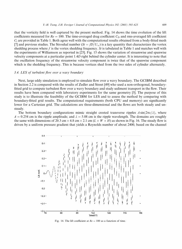
that the vorticity field is well captured by the present method. Fig. 14 shows the time evolution of the lift

coefficients measured for Re ¼ 100. The time-averaged drag coefficient CD and rms-averaged lift coefficient

Cl are provided in Table 1. Both agree well with the computational results obtained from a body-fitted mesh[7] and previous studies. The Strouhal number (St ¼ fD=U1) is a key quantity that characterizes the vortex

shedding process where f is the vortex shedding frequency. St is tabulated in Table 1 and matches well with

the experiments of Williamson as reported in [25]. Fig. 15 shows the variation of streamwise and spanwise

velocity components at a particular point 1:4D right behind the cylinder center. It is interesting to note that

the oscillation frequency of the streamwise velocity component is twice that of the spanwise component

which is the shedding frequency. This is because vortices shed from the two sides of cylinder alternately.

3.4. LES of turbulent flow over a wavy boundary

Next, large eddy simulation is employed to simulate flow over a wavy boundary. The GCIBM described

in Section 2.2 is compared with the results of Zedler and Street [49] who used a non-orthogonal, boundary-

fitted grid to compute turbulent flow over a wavy boundary and study sediment transport in the flow. Theirresults have been compared with laboratory experiments for the same geometry [5]. The purpose of this

study is to illustrate the feasibility of the GCIBM for LES and to assess the method by comparing with

boundary-fitted grid results. The computational requirements (both CPU and memory) are significantly

lower for a Cartesian grid. The calculations are three-dimensional and the flows are both steady and un-

steady.

The bottom boundary configurations mimic straight crested transverse ripples A sinð2px=kÞ, where

A ¼ 0:254 cm is the ripple amplitude; and k ¼ 5:08 cm is the ripple wavelength. The domains are roughly

the same with dimensions of 20.3 cm� 4.8 cm� 2.1 cm (L� W � H ) as shown in Fig. 16. The steady flow isdriven by a uniform pressure gradient that yields a Reynolds number of about 2400, based on the channel

Fig. 14. The lift coefficient at Re ¼ 100 as a function of time.

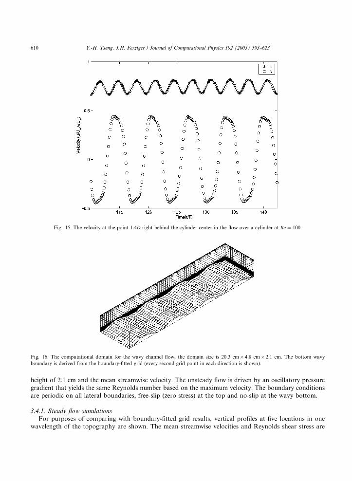
Fig. 15. The velocity at the point 1:4D right behind the cylinder center in the flow over a cylinder at Re ¼ 100.

Fig. 16. The computational domain for the wavy channel flow; the domain size is 20.3 cm� 4.8 cm� 2.1 cm. The bottom wavy

boundary is derived from the boundary-fitted grid (every second grid point in each direction is shown).


height of 2.1 cm and the mean streamwise velocity. The unsteady flow is driven by an oscillatory pressure

gradient that yields the same Reynolds number based on the maximum velocity. The boundary conditions

are periodic on all lateral boundaries, free-slip (zero stress) at the top and no-slip at the wavy bottom.

3.4.1. Steady flow simulations

For purposes of comparing with boundary-fitted grid results, vertical profiles at five locations in one

wavelength of the topography are shown. The mean streamwise velocities and Reynolds shear stress are


compared in Figs. 17(a) and (b), respectively. The differences between the IBM and boundary-fitted profiles

for the mean streamwise velocities are very small. In particular, the profiles in the outer regions (beyond

ðy � y0Þ ¼ 0:3h, y0 being the height of bottom topography) identified by Calhoun and Street [5] are almostidentical. A detailed comparison of the mean streamwise velocities in the vicinity of the crest is shown in

Fig. 18. The differences between the average velocity profiles over the crest are small. The Reynolds stress

Fig. 18. Comparisons of streamwise velocity profile between the IBM and boundary-fitted grid results for steady flow in the vicinity of

the crest. s, boundary-fitted grid results and �, IBM results.

Fig. 17. (a) Comparisons of streamwise velocity profile from the IBM and boundary-fitted grid results for steady flow. The arrow at

the top denotes 0.1 m/s (0.56Umax). (b) Comparisons of turbulent Reynolds stress between the IBM and boundary-fitted grid results for

steady flow. The arrow at the top denotes 0.0002 m2/s2. s, boundary-fitted grid results and *, IBM results.


(�u0v0) at each location in the simulation using IBM compares well with the corresponding boundary-fitted

grid profile (Fig. 17(b)).

The contours of mean vertical velocity from the IBM and boundary-fitted grid results are compared inFig. 19. The agreement is very good. Positive velocity is denoted by solid contours and negative velocity by

dashed ones. The vertical velocity is more sensitive to the method than the streamwise velocity since its

magnitude is much smaller. The recirculation is apparent in the mean vertical velocity contour as positive

vertical velocities on the downward sloping portion of the surface. The vertical velocity contours obtained

with the IBM are very similar to the contours produced by the boundary-fitted grid.

In order to illustrate the structure of the instantaneous vortex cores we have plotted contours of the

second invariant of the velocity gradient tensor [20] in Fig. 20. This approach is a variant of the pressure

minimum method. The vortex cores resemble those in channel flow, but they are longer, taller and have agreater angle of inclination [5]. These vortices result from the G€oortler instability associated with boundary

curvature. A detailed description of these vortices can be found in previous studies [5,49]. The current

study identifies the same structures, indicating that this method adequately resolves turbulent boundary

layer.

Contours of the components of the turbulence intensity (TI) are shown in Fig. 21. The maximum

streamwise u02 is found above the center of the trough and is associated with the shear layer that detaches

from the surface at the separation point. Contours of the vertical TI show that the maximum is located

slightly downstream of the location of the maximum of the streamwise TI. The maximum value is aboutone-third of the streamwise value. Henn and Sykes [18] noted an increase in spanwise velocity fluctuations

on the upstream slopes of their wavy boundary and suggested that the precise mechanism responsible is not

yet known. Calhoun and Street [5] concluded that G€oortler instability appears to be important in the for-

mation of the vortices and associated with the increase in spanwise velocity fluctuation. As shown in

Fig. 21(b), the spanwise TI shows a marked increase on the upslope close to the wavy surface. The mag-

nitude and location suggest a localized production mechanism associated with the waviness of the

boundary. These features confirm the link between the streamwise vortices and the increase of spanwise TI

found by Calhoun and Street [5].

Fig. 19. Comparisons of mean vertical velocity contours between the IBM and boundary-fitted grid results for steady flow over one

wavelength of the topography. (a) IBM (b) boundary-fitted grid. – –, negative velocity and –, positive velocity.

Fig. 20. Instantaneous snapshot of vortex cores plotted as isocontours of k2 ¼ �50 in fully developed steady wavy flow with the IBM

approach.

Fig. 21. Contours of mean flow turbulence intensity. (a) Streamwise turbulence intensity u02. (b) Spanwise turbulence intensity v02. (c)Vertical turbulence intensity w02.


3.4.2. Unsteady flow simulations

We also simulated the unsteady flow over a wavy boundary produced by an oscillatory pressure gra-

dient. A small recirculation zone forms just before the pressure gradient has attained its maximum negativevalue. As the flow slows down due to the adverse pressure gradient, spanwise vortices form and are lifted off


the bottom to roughly the height of the wave crests. Quantitative comparisons between the IBM approach

and boundary-fitted grid results of the spanwise-averaged streamwise velocity at four time steps are given in

Fig. 22. These velocity profiles are phase averaged over 10 cycles to obtain stable statistics. Sample takingstarts after the flow reaches an oscillatory steady state. The mean profiles show good agreement with

boundary-fitted simulations.

Fig. 23 provides the instantaneous, spanwise-averaged velocity vector field at t ¼ 0:25T . The time t ¼ 0

corresponds to the maximum pressure gradient. Recirculation zones appear behind the ripple crests in the

instantaneous velocity vector plot but are confined to the bottom few grid points. These are similar to

vortices obtained with boundary-fitted grids [49]. The flow behavior in both the steady and unsteady cases

in the current study is nearly the same as that in studies that used boundary-fitted grids [5,49], indicating

that the present method accurately captures the three-dimensional turbulent flow field.

Fig. 22. Comparison of streamwise velocity at different time steps. (a) t ¼ 0:25T ; (b) t ¼ 0:5T ; (c) t ¼ 0:75T and (d) t ¼ T . T is the time

period imposed by the oscillatory pressure gradient. s denotes the boundary-fitted grid result and * denotes the IBM result.

Fig. 23. Instantaneous, spanwise-averaged velocity vector plot at t ¼ 0:25T using IBM (every second grid point in each direction is

shown).


Fig. 24 presents the vortex formation/transport process by showing the vortex cores at different time

steps. The formation cycle occurs twice per period, once on either side of a wave trough. It starts as the flow

accelerates (t=T ¼ 0:25) and forms the recirculation zone. The vortex structures are generated by boundarylayer separation and the growth of three-dimensional disturbances [39]. These structures are advected

downstream as the flow slows down. The boundary layer on the lee side thickens and the recirculation zone

is lifted from the bottom. Some of the vortices are centered over the trough. This structure breaks up into a

more complex, three-dimensional structure as the flow slows further. After the flow switches direction

(t=T ¼ 0:5), these complex structures are lifted off the bottom and advected over the crest (Fig. 24(c)). They

are stretched in the streamwise direction and lose some of their strength as the flow accelerates in the other

direction (t=T ¼ 0:75). Then the process repeats in the other direction. The current results are very similar

to those simulated in [39] and the nonlinear effects appear important for the growth of three-dimensionalinstability.

4. Geophysical flow over a three-dimensional Gaussian bump

In the previous section, we validate the ghost cell approach using an uniform flow over a cylinder and a

turbulent flow over wavy boundary. In the final example, we extend the current approach to a realistic

geophysical application. The numerical experiment attempts to test the approach in the presence of three-dimensional topography and validate the GCIBM module in an existing general ocean model.

4.1. Model description

To test the flexibility of GCIBM, we use the existing MIT Global Circulation Model (MITGCM) to

simulate a geophysical flow over a three-dimensional Gaussian bump. The MITGCM is an incompressible,

finite volume, second order accurate, z-coordinate ocean model [30]. The equations are written out in full in

[30]. Adcroft et al. [1] presented two alternatives to the stair-step representation of topography in MIT-

GCM, shaved-cell and partial-cell methods. Both alternatives allow the boundary to intersect a grid of cells

by modifying the shape of those cells intersected. The shaved-cell method allows the topography to take a

piecewise linear representation and the partial-cell method uses a simpler piecewise constant representation.

Both methods show dramatic improvements in solution compared to the traditional stair-step represen-tation. The shaved-cell approach performs slightly better than partial-cell approach. However, the storage

requirements for the former are excessive and the implementation is much more complicated so the simpler

partial-cell method is provided in the MITGCM code. The shaved-cell method is essentially the same as

Fig. 24. Vortex structures plotted with the k2 method for different flow phases during a time period T (t=T ¼ 0:3 to 1.3). t=T ¼ 0; 1

corresponds to the phase of maximum oscillatory pressure gradient. The vortices are localized between two contiguous wave crests: (a)

t=T ¼ 0:3; (b) t=T ¼ 0:5; (c) t=T ¼ 0:7; (d) t=T ¼ 0:9; (e) t=T ¼ 1:1; (f) t=T ¼ 1:3.



that proposed in [46] for engineering applications. In the current validation, we compare the GCIBM

approach with both stair-step and partial-cell methods.

4.2. Model setup

The model configuration is the same as the three-dimensional test case provided in [1]. A three-di-

mensional Gaussian bump is placed in a periodic channel of length 400 km and width 300 km. The oceandepth is 4.5 km. The bump has a characteristic horizontal length scale of 25 km and is centered in the

channel. It rises to a height of 90% the depth of the ocean. The setup is essentially a typical seamount

problem. For example, Fieberling seamount is a topographic feature in the Pacific Ocean that looks very

much like a Gaussian bump.

The model is initialized with a barotropic inflow of 25 cm/s. A periodic boundary condition is used in the

streamwise direction. Some parameters are shown in Table 2. Eight equally spaced levels are chosen in the

vertical and the stratification is initially linear. A high resolution simulation run with 24 vertical levels

(Nx � Ny � Nz ¼ 240� 180� 24) is used to verify the simulation results. The high resolution case uses thepartial-cell approach to represent the bottom topography.

4.3. Simulation results

The flow is deflected to the left as it passes over the bump due to the effect of the Coriolis force and a

cyclonic eddy forms behind the seamount. In time, an anti-cyclone is formed and the first eddy is shed and

advected downstream. The stratification is strong so that the wake structure is similar to that of a two-

dimensional wake in each layer. The three-dimensional structure of the cyclonic eddy at t ¼ 10 days in

terms of the iso-contour of relative vorticity with f ¼ 0:2fmax from the high resolution simulation is shown

in Fig. 25. Only positive vorticity (cyclone) is shown. Fig. 26 shows the non-dimensional depth integrated

relative vorticity (f=f ) at t ¼ 10 days. We use this high resolution result as the standard.

Fig. 27 shows the comparison of the results between the stair-step grid and the IBM implementation for5-km resolution (Nx � Ny � Nz ¼ 80� 60� 8). The effect of the topography in steering the flow is very

similar in the two results. The distortion of the cyclonic tail, upstream of the bump, is a result of the cy-

clonic eddy impinging on the inflow region and should be ignored. The orientation of the elliptic cyclonic

eddy is slightly different but the processes of eddy formation, shedding and advection seen in the IBM

modification (Fig. 27(b)) are quite close to those observed in the high resolution simulation. The high

resolution solution is smoother than the model solution. Very little difference is observed between the IBM

Table 2

Parameters for the numerical simulation of flow over a three-dimensional Gaussian bump

MITGCM

Channel length (km) 400

Channel width (km) 300

Nominal ocean depth H (m) 4500

Height of bump h (m) 4050

Length scale of bump L (m) 25

Stratification NH=fL 1.5

Barotropic inflow ui (cm/s) 25

Horizontal biharmonic viscosity (m4/s) 5� 109

Vertical Laplacian viscosity (m2/s) 1� 10�3

Horizontal biharmonic diffusion (m4/s) 1� 109

Vertical diffusion (m2/s) 1� 10�5

Fig. 25. The three-dimensional structure of iso-contour of relative vorticity f ¼ 0:2fmax at t ¼ 10 days.

Fig. 26. Non-dimensional depth integrated relative vorticity f=f at t ¼ 10 days at fine grid resolution (Nx � Ny � Nz ¼ 240� 180� 24).


and high resolution simulations in Fig. 26. These include the larger maximum within the tail and the

smoother solution in the high resolution case. On the whole, the solutions are qualitatively similar. Despite

the differences, it is clear that the IBM method does a creditable job in representing the flow over this large

topographic feature. The difference between the solutions using IBM and the stair-step grid are significant.

There is a stronger local maximum within the tail in the IBM solution. The stair-step grid result has a much

wider shed cyclonic vortex. In addition, we observe much more small-scale noise near the bump in the stair-

step solution.

Fig. 27. Contours of non-dimensional depth integrated relative vorticity f=f at t ¼ 10 days at horizontal resolution Dx ¼ 5 km: (a)

stair-step representation of topography and (b) IBM representation of topography (Nx � Ny � Nz ¼ 80� 60� 8).


We also conducted two additional simulations for each topography representation in order to test the

convergence property. Figs. 28 and 29 show the solutions for two finer resolutions of Dx ¼ 2:5 and

Dx ¼ 1:67 km, respectively. We keep the vertical resolution unchanged. The solutions differ from the ori-

ginal calculations (Fig. 27) only in fine detail, the overall structure being the same. The amplitude of the

cyclonic eddy increases as the resolution is made finer, suggesting that coarse resolution underestimates the

eddy strength. As we increase the horizontal resolution (i.e., reduce Dx, Dy only), the IBM solutions

converge to the correct solution. In the case of the stair-step grid, as the resolution is increased, the noise

near the bump increases and the cyclonic eddy is distorted. The �rings� of grid-scale noise become morepronounced with increased resolution.

Fig. 28. Contours of nondimensional depth integrated relative vorticity f=f at t ¼ 10 days at horizontal resolution Dx ¼ 2:5 km: (a)


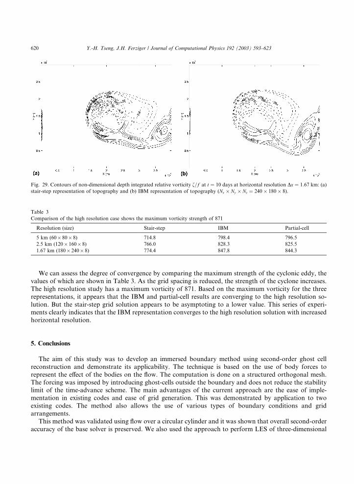
Fig. 29. Contours of non-dimensional depth integrated relative vorticity f=f at t ¼ 10 days at horizontal resolution Dx ¼ 1:67 km: (a)


Table 3

Comparison of the high resolution case shows the maximum vorticity strength of 871

Resolution (size) Stair-step IBM Partial-cell

5 km (60� 80� 8) 714.8 798.4 796.5

2.5 km (120� 160� 8) 766.0 828.3 825.5

1.67 km (180� 240� 8) 774.4 847.8 844.3


We can assess the degree of convergence by comparing the maximum strength of the cyclonic eddy, the

values of which are shown in Table 3. As the grid spacing is reduced, the strength of the cyclone increases.

The high resolution study has a maximum vorticity of 871. Based on the maximum vorticity for the three

representations, it appears that the IBM and partial-cell results are converging to the high resolution so-

lution. But the stair-step grid solution appears to be asymptoting to a lower value. This series of experi-

ments clearly indicates that the IBM representation converges to the high resolution solution with increased

horizontal resolution.

5. Conclusions

The aim of this study was to develop an immersed boundary method using second-order ghost cell

reconstruction and demonstrate its applicability. The technique is based on the use of body forces to

represent the effect of the bodies on the flow. The computation is done on a structured orthogonal mesh.

The forcing was imposed by introducing ghost-cells outside the boundary and does not reduce the stabilitylimit of the time-advance scheme. The main advantages of the current approach are the ease of imple-

mentation in existing codes and ease of grid generation. This was demonstrated by application to two

existing codes. The method also allows the use of various types of boundary conditions and grid

arrangements.

This method was validated using flow over a circular cylinder and it was shown that overall second-order

accuracy of the base solver is preserved. We also used the approach to perform LES of three-dimensional


turbulent flow over a wavy boundary. Both steady and unsteady flows are simulated and compared with

established numerical simulations done on a boundary-fitted grid. The results agree very well with the

previous numerical and experimental results, indicating the validity and accuracy of the present method.Finally, we implemented the method in an existing ocean model and compared with a high resolution case

and partial-cell simulation. The comparison among the IBM, partial-cell and stair-step representations

clearly indicates that the IBM results are comparable to those obtained with partial cells. The ghost-cell

approach can be readily applied to any existing code.

Use of a more realistic boundary condition (e.g., log-law) is being investigated in order to broaden the

applicability of the method. A method for accurate representation of rough boundary is needed. Cui et al.

[6] proposed a force field model to simulate turbulent flow over rough wavy surface. An arbitrary roughness

can be decomposed into resolved-scale and subgrid-scale roughness [34]. Roughness was represented usingboundary forcing by Verzicco et al. [44]. Their results could not reproduce the mean velocity in the near-

wall region and the force field model requires an empirical drag coefficient. Further analysis is needed to

better represent a rough boundary using the IBM. In another publication, we will also extend the method to

the simulation of the flow in Monterey Bay, California.

Acknowledgements

The authors thank Prof. Robert L. Street and Dr. Emily Zedler for their invaluable help and continuous

support with the turbulent flow simulation; Prof. Paul Durbin and Gianluca Iaccarino for their useful

discussion; Dr. S. Majumdar for providing the two-dimensional flow over circular cylinder data; and Dr. A.

Adcroft for providing the MITGCM code. Financial support for this work was provided by NSF ITR/AP

(GEO) grant number 0113111 (Ms. B. Fossum, Program Manager) and the NASA AMES/Stanford Center

for Turbulent Research.

References

[1] A. Adcroft, C. Hill, J. Marshall, Representation of topography by shaved cells in a height coordinate ocean model, Mon. Weather

Rev. 125 (9) (1997) 2293–2315.

[2] A.S. Almgren, J.B. Bell, P. Colella, T. Marthaler, A cartesian grid projection method for the incompressible Euler equations in

complex geometries, SIAM J. Sci. Comput. 18 (5) (1997) 1289–1309.

[3] D. Calhoun, A cartesian grid method for solving the two-dimensional streamfunction-vorticity equations in irregular regions,

J. Comput. Phys. 176 (2) (2002) 231–275.

[4] D. Calhoun, R.J. LeVeque, A cartesian grid finite-volume method for the advection–diffusion equation in irregular geometries,

J. Comput. Phys. 157 (1) (2000) 143–180.

[5] R.J. Calhoun, R.L. Street, Turbulent flow over a wavy surface: neutral case, J. Geophys. Res. 106 (2001) 9277–9293.

[6] J. Cui, V.C. Patel, C.L. Lin, Prediction of turbulent flow over rough surfaces using a force field in large eddy simulation, ASME J.

Fluid Engrg. 125 (1) (2003) 2–9.

[7] A. Dias, S. Majumdar, Numerical computation of flow around a circular cylinder, Technical Report, PS II Report, BITS Pilani,

India.

[8] E.A. Fadlun, R. Verzicco, P. Orlandi, J. Mohd-Yusof, Combined immersed-boundary finite-difference methods for three-

dimensional complex flow simulations, J. Comput. Phys. 161 (2000) 30–60.

[9] R.P. Fedkiw, Coupling an Eulerian fluid calculation to a Lagrangian solid calculation with the ghost fluid method, J. Comput.

Phys. 175 (2002) 200–224.

[10] R.P. Fedkiw, T. Aslam, B. Merriman, S. Osher, A non-oscillatory Eulerian approach to interfaces in multimaterial flows (the

ghost fluid method), J. Comput. Phys. 152 (1999) 457–492.

[11] J.H. Ferziger, M. Peri�cc, Computational Methods for Fluid Dynamics, third ed., Springer Verlag, Berlin, Heidelberg, 2001.

[12] H. Forrer, R. Jeltsch, A higher-order boundary treatment for Cartesian-grid method, J. Comput. Phys. 140 (1998) 259–277.

[13] R. Franke, Scattered data interpolation: tests of some methods, Math. Comput. 38 (1982) 181–200.


[14] F. Gibou, R.P. Fedkiw, L.T. Cheng, M. Kang, A second-order-accurate symmetric discretization of the Poisson equation on

irregular domains, J. Comput. Phys. 176 (2002) 205–227.

[15] D. Goldstein, R. Handler, L. Sirovich, Modeling a no-slip flow boundary with an external force field, J. Comput. Phys. 105 (1993)

354–366.

[16] G.H. Golub, C.F. van Loan, Matrix Computations, third ed., The Johns Hopkins University Press, Baltimore, 1996.

[17] D.C. Haworth, K. Jansen, Large-eddy simulation on unstructured deforming meshes: towards reciprocating IC engines, Comput.

Fluids 29 (2000) 493–524.

[18] D. Henn, I. Sykes, Large-eddy simulation of flow over wavy surfaces, J. Fluid Mech. 383 (1999) 75–112.

[19] G. Iaccarino, R. Verzicco, Immersed boundary technique for turbulent flow simulations, Appl. Mech. Rev. 56 (2003) 331–347.

[20] J. Jeong, F. Hussain, On the identification of a vortex, J. Fluid Mech. 285 (1995) 69–94.

[21] H. Johansen, P. Colella, A cartesian grid embedded boundary method for poisson�s equation on irregular domains, J. Comput.

Phys. 147 (1) (1998) 60–85.

[22] J. Kim, D. Kim, H. Choi, An immersed-boundary finite-volume method for simulations of flow in complex geometries, J. Comput.

Phys. 171 (2001) 132–150.

[23] J. Kim, P. Moin, Application of a fractional-step method to incompressible Navier–Stokes equations, J. Comput. Phys. 59 (1985)

308–323.

[24] M.P. Kirkpatrick, S.W. Armfield, J.H. Kent, A representation of curved boundaries for the solution of the Navier–Stokes

equations on a staggered three-dimensional cartesian grid, J. Comput. Phys. 184 (1) (2003) 1–36.

[25] M. Lai, C.S. Peskin, An immersed boundary method with formal second-order accuracy and reduced numerical viscosity,

J. Comput. Phys. 160 (2000) 705–719.

[26] B.P. Leonard, A stable and accurate convective modeling procedure based on quadratic upstream interpolation, Comput.

Methods Appl. Mech. Engrg. 19 (1979) 58–98.

[27] R.J. LeVeque, J. Oliger, Numerical-methods based on additive splittings for hyperbolic partial-differential equations, Math.

Comp. 40 (1983) 469–497.

[28] X.D. Liu, R.P. Fedkiw, M.J. Kang, A boundary condition capturing method for Poisson�s equation on irregular domains,

J. Comput. Phys. 160 (1) (2003) 151–178.

[29] S. Majumdar, G. Iaccarino, P. Durbin, RANS solvers with adaptive structured boundary non-conforming grids, in: Annual

Research Briefs, NASA Ames Research Center/Stanford University Center for Turbulence Research, Stanford, CA, 2001, pp.

353–366.

[30] J. Marshall, C. Hill, L. Perelman, A. Adcroft, Hydrostatic; quasi-hydrostatic; and nonhydrostatic ocean modeling, J. Geophys.

Res. 102 (C3) (1997) 5733–5752.

[31] P. McCorquodale, P. Colella, H. Johansen, A cartesian grid embedded boundary method for the heat equation on irregular

domains, J. Comput. Phys. 173 (2) (2001) 620–635.

[32] A. McKenney, L. Greengard, A. Mayo, A fast Poisson solver for complex geometries, J. Comput. Phys. 118 (2) (1995) 348–355.

[33] J. Mohd-Yusof, Combined immersed boundary/B-spline methods for simulations of flows in complex geometries, in: Annual

Research Briefs, NASA Ames Research Center/Stanford University Center for Turbulence Research, Stanford, CA, 1997, pp.

317–327.

[34] A. Nakayama, K. Sakio, Simulation of flows over wavy rough boundaries, in: Annual Research Briefs, NASA Ames Research

Center/Stanford University Center for Turbulence Research, Stanford, CA, 2002, pp. 313–324.

[35] R.B. Pember, J.B. Bell, P. Colella, W.Y. Crutchfield, M.L. Welcome, An adaptive Cartesian grid method for unsteady

compressible flow in irregular regions, J. Comput. Phys. 120 (2) (1995) 278–304.

[36] C.S. Peskin, Flow patterns around heart valves: a numerical method, J. Comput. Phys. 10 (1972) 252–271.

[37] Y. Saad, Iterative Methods for Sparse Linear Systems, PWS Publishing Company, Boston, 1996.

[38] E.M. Saiki, S. Biringen, Numerical simulation of a cylinder in uniform flow: application of a virtual boundary method, J. Comput.

Phys. 123 (1996) 450–465.

[39] P. Scandura, G. Vittori, P. Blondeaux, Three-dimensional oscillatory flow over steep ripples, J. Fluid Mech. 412 (2000) 355–378.

[40] H.L. Stone, Iterative solution of implicit approximations of multidimensional partial differential equations, SIAM J. Numer.

Anal. 5 (1968) 530–558.

[41] Y.H. Tseng, J.H. Ferziger, Effects of coastal geometry and the formation of cyclonic/anti-cyclonic eddies on turbulent mixing in

upwelling simulation, J. Turbulence 2 (2001) 014.

[42] H.S. Udaykumar, R. Mittal, P. Rampunggoon, A. Khanna, A sharp interface Cartesian grid method for simulating flows with

complex moving boundaries, J. Comput. Phys. 174 (2001) 345–380.

[43] R. Verzicco, G. Iaccarino, M. Fatica, P. Orlandi, Flow in an impeller stirred tank using an immersed boundary method, in:

Annual Research Briefs, NASA Ames Research Center/Stanford University Center for Turbulence Research, Stanford, CA, 2000,

pp. 251–261.

[44] R. Verzicco, J. Mohd-Yusof, P. Orlandi, D. Haworth, Large Eddy simulation in complex geometry configurations using boundary

body forces, AIAA J. 38 (2000) 427–433.


[45] S.J. Xu, T. Aslam, D.S. Stewart, High resolution numerical simulation of ideal and non-ideal compressible reacting flows with

embedded internal boundaries, Combust. Theory Model. 1 (1) (1997) 113–142.

[46] T. Ye, R. Mittal, H.S. Udaykumar, W. Shyy, An accurate Cartesian grid method for viscous incompressible flows with complex

immersed boundaries, J. Comput. Phys. 156 (1993) 209–240.

[47] Y. Zang, R.L. Street, J.R. Koseff, A dynamic mixed subgrid-scale model and its application to turbulent recirculating flows, Phys.

Fluids A5 (1993) 3186–3196.

[48] Y. Zang, R.L. Street, J.R. Koseff, A non-staggered grid, fractional step method for time-dependent incompressible Navier–Stokes

equations in curvilinear coordinates, J. Comput. Phys. 114 (1994) 18–33.

[49] E.A. Zedler, R.L. Street, Large-Eddy simulation of sediment transport: currents over ripples, J. Hydraul. Engrg. 127 (2001) 444–

452.

a ghost-cell immersed boundary method for flow in complex geometry

Documents