a geometric study of superintegrable systems arxiv:1209
TRANSCRIPT

A Geometric Study of Superintegrable
Systems
by
Amelia L. Yzaguirre
Submitted in partial fulfillment of the requirements
for the degree of Master of Science
at
Dalhousie University
Halifax, Nova Scotia
August 2012
c© Copyright by Amelia L. Yzaguirre, 2012
arX
iv:1
209.
5672
v1 [
mat
h-ph
] 2
5 Se
p 20
12

Acknowledgements
My sincerest gratitude extends to my boyfriend, Antonio, who has pro-
vided me with love and light throughout the development of this thesis
and beyond. His support has kept me afloat in the most treacherous of
storms, and I thank him immensely for being such a source of inspiration.
I also thank my parents, brothers, and sister for providing encouragement
and expressing enthusiasm in my work while I have been so far away from
home. I miss you all beyond words. Last but not least I want to thank my
advisor Dr. Roman Smirnov for his unbelievable patience and guidance
during this study.
This material is based upon work supported by the National Science Foun-
dation Graduate Research Fellowship under Grant No. 1048093. Any
opinion, findings, and conclusions or recommendations expressed in this
material are my own, and do not necessarily reflect the views of the Na-
tional Science Foundation.
I dedicate the work in this thesis to the passing of my best friend, Kraven.
I think of you every day.

Abstract
Superintegrable systems are classical and quantum Hamiltonian systems
which enjoy much symmetry and structure that permit their solubility
via analytic and even, algebraic means. They include such well-known
and important models as the Kepler potential, Calogero-Moser model,
and harmonic oscillator, as well as its integrable perturbations, for exam-
ple, the Smorodinsky-Winternitz (SW) potential. Normally, the problem
of classification of superintegrable systems is approached by considering
associated algebraic, or geometric structures. To this end, we invoke the
invariant theory of Killing tensors (ITKT). Through the ITKT, and in
particular, the recursive version of the Cartan method of moving frames
to derive joint invariants, we are able to intrinsically characterise and in-
terpret the arbitrary parameters appearing in the general form of the SW
superintegrable potential. Specifically, we determine, using joint invari-
ants, that the more general the geometric structure associated with the
SW potential is, the fewer arbitrary parameters it admits. Additionally,
we classify the multi-separability of a recently discovered superintegrable
system which generalizes the SW potential and is dependent on an addi-
tional arbitrary parameter k, known as the Tremblay-Turbiner-Winternitz
(TTW) system. We provide a proof that only for the case k = ±1 does
the general TTW system admit orthogonal separation of variables with
respect to both Cartesian and polar coordinates.

Contents
Contents iii
List of Figures v
List of Symbols vi
1 Introduction 1
1.1 Summary of Results . . . . . . . . . . . . . . . . . . . . . . . . . . . 5
1.2 Overview and Historical Development . . . . . . . . . . . . . . . . . . 6
1.3 Notation and Conventions . . . . . . . . . . . . . . . . . . . . . . . . 9
1.3.1 Tensors and Index Notation . . . . . . . . . . . . . . . . . . . 11
1.3.2 The Lie Bracket and its Generalisation . . . . . . . . . . . . . 14
1.3.3 Poisson Manifolds . . . . . . . . . . . . . . . . . . . . . . . . . 16
2 Theoretical Overview 18
2.1 Hamiltonian Mechanics . . . . . . . . . . . . . . . . . . . . . . . . . . 18
2.2 Hamilton-Jacobi Theory . . . . . . . . . . . . . . . . . . . . . . . . . 24
2.3 Separability on the Euclidean Plane . . . . . . . . . . . . . . . . . . . 28
2.4 Invariant Theory of Killing Tensors . . . . . . . . . . . . . . . . . . . 32
2.4.1 Preliminaries . . . . . . . . . . . . . . . . . . . . . . . . . . . 33
2.4.2 The Moving Frames Method . . . . . . . . . . . . . . . . . . . 38
2.4.3 Joint Invariants of Killing Tensors . . . . . . . . . . . . . . . . 42
3 Superintegrable Systems on the Euclidean Plane 47
3.1 Development of Superintegrable Systems . . . . . . . . . . . . . . . . 47
iii

Contents
3.2 Characterisation of the Smorodinsky-Winternitz Potential . . . . . . 50
3.2.1 Weakening the Conditions . . . . . . . . . . . . . . . . . . . . 53
3.3 The Tremblay-Turbiner-Winternitz System . . . . . . . . . . . . . . . 58
4 Conclusions and Outlook 65
Bibliography 67
A Compact Formulae 75
A.1 The Action of the Isometry Group . . . . . . . . . . . . . . . . . . . 75
A.2 Kogan’s Recursive Approach . . . . . . . . . . . . . . . . . . . . . . . 76
B The Killing Tensor Equation in Local Coordinates 78
C A Complicated Trigonometric Equation 81
D Linear Independence of a Set of Functions 82
iv

List of Figures
1.1 The orthogonal coordinate webs in the Euclidean plane, in the canon-
ical position, arranged according to their number of singular points.
Clockwise from top left: elliptic-hyperbolic, parabolic, polar, and Carte-
sian. . . . . . . . . . . . . . . . . . . . . . . . . . . . . . . . . . . . . 7
1.2 Examples of orthogonal coordinate webs in the Euclidean plane, in
some general position. Clockwise from top left: elliptic-hyperbolic,
parabolic, polar, and Cartesian. . . . . . . . . . . . . . . . . . . . . . 10
2.1 Quadrilateral whose vertices are given by the singular points of two
non-degenerate orbits {KEH ,KEH} ∈ K2(E2)×K2(E2) . . . . . . . . 46
3.1 Triangle whose vertices are given by the singular points of two Killing
tensors, one non-degenerate and the other degenerate, (KEH ,KP ) ∈K2(E2)×K2(E2). In this case, KEH is in the canonical form. . . . . . 54
v
List of Symbols
En Euclidean space of dimension n . . . . . . . . . . . . . . . . . . . . . . . . . . . . . . . . . . . . . 5
Rn n-dimensional Cartesian space . . . . . . . . . . . . . . . . . . . . . . . . . . . . . . . . . . . . 11
M Pseudo-Riemannian manifold of dimension n . . . . . . . . . . . . . . . . . . . . . . 6
g Metric tensor . . . . . . . . . . . . . . . . . . . . . . . . . . . . . . . . . . . . . . . . . . . . . . . . . . . . . . 9
Tp(M) Tangent space of M at a point p . . . . . . . . . . . . . . . . . . . . . . . . . . . . . . . . . . . 9
T (M) Tangent bundle of M . . . . . . . . . . . . . . . . . . . . . . . . . . . . . . . . . . . . . . . . . . . . . . 9
T ∗p (M) Cotangent space of M at a point p . . . . . . . . . . . . . . . . . . . . . . . . . . . . . . . . 9
T ∗(M) Cotangent bundle of M . . . . . . . . . . . . . . . . . . . . . . . . . . . . . . . . . . . . . . . . . . . .9
T sr Tensor of valence (s, r) . . . . . . . . . . . . . . . . . . . . . . . . . . . . . . . . . . . . . . . . . . . .11
εij Levi-civita symbol . . . . . . . . . . . . . . . . . . . . . . . . . . . . . . . . . . . . . . . . . . . . . . . . 10
δij Kronecker delta . . . . . . . . . . . . . . . . . . . . . . . . . . . . . . . . . . . . . . . . . . . . . . . . . . .11
Γijk Christoffel symbol . . . . . . . . . . . . . . . . . . . . . . . . . . . . . . . . . . . . . . . . . . . . . . . . 14
H Hamiltonian . . . . . . . . . . . . . . . . . . . . . . . . . . . . . . . . . . . . . . . . . . . . . . . . . . . . . . . 6
F First integral of motion . . . . . . . . . . . . . . . . . . . . . . . . . . . . . . . . . . . . . . . . . . . 29
pi Momenta coordinates . . . . . . . . . . . . . . . . . . . . . . . . . . . . . . . . . . . . . . . . . . . . . . 5
qi Position coordinates . . . . . . . . . . . . . . . . . . . . . . . . . . . . . . . . . . . . . . . . . . . . . . . 5
L Lagrangian function . . . . . . . . . . . . . . . . . . . . . . . . . . . . . . . . . . . . . . . . . . . . . . 19
S Action function . . . . . . . . . . . . . . . . . . . . . . . . . . . . . . . . . . . . . . . . . . . . . . . . . . . 19
XH Hamiltonian vector field . . . . . . . . . . . . . . . . . . . . . . . . . . . . . . . . . . . . . . . . . . 17
P0 Canonical Poisson bivector . . . . . . . . . . . . . . . . . . . . . . . . . . . . . . . . . . . . . . . .16
Xi Translational basis vector . . . . . . . . . . . . . . . . . . . . . . . . . . . . . . . . . . . . . . . . . 34
R Rotational basis vector . . . . . . . . . . . . . . . . . . . . . . . . . . . . . . . . . . . . . . . . . . . 34
K Killing tensor of valence two . . . . . . . . . . . . . . . . . . . . . . . . . . . . . . . . . . . . . . . 5
Kp(M) Vector space of valence p Killing tensors defined on M . . . . . . . . . . . . 16
vi

List of Symbols
Kp(M)/G Quotient space . . . . . . . . . . . . . . . . . . . . . . . . . . . . . . . . . . . . . . . . . . . . . . . . . . . .39
SE(n) Special Euclidean group . . . . . . . . . . . . . . . . . . . . . . . . . . . . . . . . . . . . . . . . . . 35
SO(n) Special orthogonal group . . . . . . . . . . . . . . . . . . . . . . . . . . . . . . . . . . . . . . . . . .35
� Acting on . . . . . . . . . . . . . . . . . . . . . . . . . . . . . . . . . . . . . . . . . . . . . . . . . . . . . . . . .35
dim Dimension . . . . . . . . . . . . . . . . . . . . . . . . . . . . . . . . . . . . . . . . . . . . . . . . . . . . . . . . 33(nk
)Number of k−subsets of n elements . . . . . . . . . . . . . . . . . . . . . . . . . . . . . . . 33
d2( , ) Distance function . . . . . . . . . . . . . . . . . . . . . . . . . . . . . . . . . . . . . . . . . . . . . . . . . 45⊔Disjoint union . . . . . . . . . . . . . . . . . . . . . . . . . . . . . . . . . . . . . . . . . . . . . . . . . . . . . 9
⊗ Tensor product . . . . . . . . . . . . . . . . . . . . . . . . . . . . . . . . . . . . . . . . . . . . . . . . . . . 13
� Symmetric tensor product . . . . . . . . . . . . . . . . . . . . . . . . . . . . . . . . . . . . . . . . 13
∧ Wedge product . . . . . . . . . . . . . . . . . . . . . . . . . . . . . . . . . . . . . . . . . . . . . . . . . . . 13
× Cartesian product . . . . . . . . . . . . . . . . . . . . . . . . . . . . . . . . . . . . . . . . . . . . . . . . 42
d Exterior derivative operator . . . . . . . . . . . . . . . . . . . . . . . . . . . . . . . . . . . . . . . . 3
L Lie derivative operator . . . . . . . . . . . . . . . . . . . . . . . . . . . . . . . . . . . . . . . . . . . . 15
∇ Covariant derivative operator . . . . . . . . . . . . . . . . . . . . . . . . . . . . . . . . . . . . . 14
[ , ] Schouten bracket . . . . . . . . . . . . . . . . . . . . . . . . . . . . . . . . . . . . . . . . . . . . . . . . . 15
{ , } Poisson bracket . . . . . . . . . . . . . . . . . . . . . . . . . . . . . . . . . . . . . . . . . . . . . . . . . . . 16
HJ Hamilton-Jacobi . . . . . . . . . . . . . . . . . . . . . . . . . . . . . . . . . . . . . . . . . . . . . . . . . . 18
SW Smorodinsky-Winternitz . . . . . . . . . . . . . . . . . . . . . . . . . . . . . . . . . . . . . . . . . . . ii
TTW Tremblay-Turbiner-Winternitz . . . . . . . . . . . . . . . . . . . . . . . . . . . . . . . . . . . . . ii
PDE Partial differential equation . . . . . . . . . . . . . . . . . . . . . . . . . . . . . . . . . . . . . . . 16
vii

Chapter 1
Introduction
The origins of this thesis can be traced back to 1965 when Winternitz and Fris
used the theory of Lie groups to classify the separable webs of the Euclidean plane.
Specifically, they computed the invariants of the second-order symmetries of the
Laplace equation
∆V (x, y) =∂2V
∂x2+∂2V
∂y2= 0,
defined on the Euclidean plane under the action of the Euclidean group. As we
shall develop in Section 2.3, the classification of such separable webs is intimately
related to the Hamilton-Jacobi theory, which provides a formulation of Hamiltonian
mechanics that allows one to conclude the solubility of a classical Hamiltonian system
(see Section 2.1). Indeed, by determining the orthogonal coordinate systems that
afford separation of variables in the corresponding Hamilton-Jacobi equation for a
Hamiltonian system (see Section 2.2), one can ultimately obtain exact solutions, or
trajectories, of the Hamiltonian system.
The work of Stackel in 1893 and its extension by Eisenhart in 1934 were both
essential to the development of this geometric approach to studying Hamiltonian
systems. Both of these canonical papers established the essential role of a geometric
object that naturally arose when studying orthogonal separation of variables of the
Hamilton-Jacobi equation: a Killing tensor of valence two. Studying the intrinsic
properties of Killing tensors corresponding to certain orthogonally separable cases
thus provided a new approach to the problem of solving a Hamiltonian system. In
1

1 Introduction
2002, McLenaghan, Smirnov, and The [45] utilised classical invariant theory to de-
velop the properties of such Killing tensors, which marked the initial stages in the
development of the invariant theory of Killing tensors. Since then the theory has
been utilised by a significant number of authors who have applied it in a more gen-
eral setting to study Killing tensors defined in spaces of constant curvature (e.g., see
[45, 17, 1, 3, 13, 12, 15, 29, 30, 31, 32, 55, 56, 70, 73] and the relevant references
therein).
In this thesis we use the invariant theory of Killing tensors in the context of solving
the classification problem for superintegrable Hamiltonian systems defined on the Eu-
clidean plane1. One system of particular interest is the Tremblay-Turbiner-Winternitz
(TTW) system introduced in 2009 [65], which is a generalisation of another super-
integrable system of interest, the Smorodinsky-Winternitz (SW) system. The unique
feature of the TTW system is that it provides an infinite family of solvable and in-
tegrable (quantum) systems on the Euclidean plane with respect to a parameter k
[65, 66, 67]. Furthermore, this family of systems was proven to be both classically
and quantum superintegrable for any rational value of k [33, 35, 36, 37].
A Hamiltonian system with n degrees of freedom is completely integrable if in
addition to its Hamiltonian, H, it admits n − 1 first integrals of motion, Fi, i =
1, . . . , n− 1, that are well-defined functions on the phase space. These first integrals
must be functionally independent,
dH ∧ dF1 ∧ . . . ∧ dFn−1 6= 0,
and in involution with respect to the Poisson bracket (see Section 1.3)
{H,Fi}P0 = {Fi, Fj}P0 = 0, i, j = 1, . . . , n− 1.
If such a completely integrable system admits additional n− 1 functionally indepen-
dent first integrals of motion, Gi, i = 1, . . . n− 1, namely
dH ∧ dF1 ∧ . . . ∧ dFn−1 ∧ dG1 ∧ . . . ∧ dGn−1 6= 0,
1The term superintegrable was introduced in 1983 by S. Wojciechowski [71].
2

1 Introduction
which are in involution
{H,Gi}P0 = {Gi, Gj}P0 = 0, i, j = 1, . . . , n− 1.
then the system is maximally superintegrable (see Section 3.1). Since such systems
have more constants of motion than degrees of freedom it is possible to integrate them
through analytic and algebraic methods. For this reason, superintegrable systems are
often sought after as starting points for studying much more complicated systems.
Some familiar examples of superintegrable systems (in the realm of physics) include
the harmonic oscillator, the Kepler system, the Calogero-Moser system, the hydrogen
atom, and others (see e.g. [7, 21, 46, 48, 58, 62]).
The construction of an infinite family of superintegrable systems, such as the TTW
system, is fairly straightforward. We demonstrate the technique with respect to the
TTW system, which begins with the second-order system defined by a Hamiltonian
(see Section 2.1), of the form
H = p2x + p2
y − ω2(x2 + y2) +α
x2+β
y2, (1.1)
where px, py denote the momenta coordinates, and x, y denote the position coordi-
nates. This is the SW system, which is recognised as a seond-order perturbation of
the two-dimensional harmonic oscillator and further, is an example of a superinte-
grable Hamiltonian system since it is multi-separable with respect to both Cartesian
and polar coordinates (see Section 2.3). The property of being superintegrable is
what we intend to retain in the construction of a new Hamiltonian system.
To this end, we can transform the Hamiltonian (1.1) to polar coordinates and
replace θ with kθ, where k is some new arbitrary parameter. Such a transformation
of course preserves the property of the system being separable with respect to polar
coordinates, though we now arrive at a new Hamiltonian of the form
H = p2r + 1
rpr +
1
r2p2θ − ω2r2 +
1
r2
(α
cos2 kθ+
β
sin2 kθ
). (1.2)
This is the TTW system. One characterising feature of the TTW system is that much
3

1 Introduction
like the system (1.1), it is still separable with respect to polar coordinates and it still
behaves as a perturbation of the harmonic oscillator. Though this development raises
the question of whether the system remains superintegrable for all values of k. In their
initial publication, Tremblay et al. [65] conjectured and provided strong evidence for
the superintegrability of this system for all rational values of k, a claim which fueled
the activity of researchers who were set out to prove its validity. Indeed, if the system
remained superintegrable then it provided an example of a second order system that
could generate an infinite number of higher order superintegrable systems, which
would work towards the development of a classification theory for superintegrable
systems. The claim was proven to be true in the classical case, where Kalnins et
al. [37] explicitly solved for the higher order first integrals, appearing as polynomials
in the momenta, by using the structure algebra of first integrals. In this context,
one must determine the order defining when the algebra of first integrals closes with
respect to the Poisson bracket, and find the corresponding structure equations for the
symmetry algebra (see [34] for more details). It was also proven in the quantum case
through a recurrence method introduced by Kalnins et al. (see e.g. [34, 35, 36]). In
this thesis we investigate whether there are values of k for which the system admits
two first integrals of motion quadratic in the momenta. Prior to this thesis, such a
result has not been shown.
In the Euclidean plane, maximal superintegrability requires that a Hamiltonian
system defined by H (see Section 2.1) admits two additional first integrals of motion,
Fi, i = 1, 2 functionally independent and in involution, meaning that
dH ∧ dF1 ∧ dF2 6= 0
and {H,Fi} = XH(Fi) = 0, for i = 1, 2. Note that a Hamiltonian is always a
first integral of motion, a property which can be physically interpreted as a system
demonstrating conservation of energy. For the system given by the Hamiltonian (1.2),
we also readily obtain a second first integral by exploiting the fact that the system
is separable with respect to polar coordinates. Indeed, since (1.2) takes the form of
a natural Hamiltonian, we can use a result by Liouville [42] which yields that such a
4

1.1 Summary of Results
system will admit a first integral of motion quadratic in the momenta according to
F (qi, pi) = 12Kij(qi)pipj + U(qi), i, j = 1, 2, (1.3)
with position coordinates qi, momenta coordinates pi, where Kij is a Killing two-
tensor whose normal eigenvectors generate the polar coordinate web (see Section
2.3), and U(qi) is a potential satisfying dU = KdV , where K = Kg−1, i.e. K is a
(1, 1)−tensor, which in component form is given by Kij := Ki`g`j. And so, in fact,
there remains only one first integral of motion to find in order for us to conclude
superintegrability of the TTW system.
1.1 Summary of Results
In this thesis we provide a new perspective on the study of joint invariants of Killing
tensors, which are objects originally defined by Smirnov and Yue in 2004 [56], and
further extended by Adlam et al. [3]. In particular, we establish a relationship be-
tween the geometric and analytic properties of superintegrable Hamiltonian systems,
defined on the Euclidean plane, E2, through the vanishing of joint invariants in the
product space K2(E2) × K2(E2), where K2(E2) denotes the vector space of Killing
two tensors defined on the Euclidean plane (see Section 2.4). We focus our study on
the characterisation of the Smorodinsky-Winternitz potential, where we can readily
establish a link between the arbitrary parameters appearing in the potential and the
parameters in the associated vector space of Killing tensors. In particular, we find
that the more structure we place on the product space K2(E2) × K2(E2), the more
general form a corresponding superintegrable potential is allowed to take, and vice
versa.
As a generalisation of the Smorodinsky-Winternitz potential, we then focus our
attention on the Tremblay-Turbiner-Winternitz potential, where we provide a defini-
tive answer to the following question:
For which values of k is the TTW system multi-separable?
Through the geometric description of a superintegrable potential provided by certain
types of Killing two-tensors (see Chapter 3.1), we find that only when k = ±1, which
5

1.2 Overview and Historical Development
in fact reduces the system to the Smorodinsky-Winternitz potential, does the TTW
system retain the property of being multi-separable, in particular, with respect to
both Cartesian and polar coordinates in the canonical position.
1.2 Overview and Historical Development
We begin with a Hamiltonian system defined (on a pseudo-Riemannian manifoldM)
by a natural Hamiltonian of the form
H(qi, pi) = 12gijpipj + V (qi), i, j = 1, 2, (1.4)
where (q,p) denote generalised canonical coordinates. A first integral of a Hamil-
tonian system is defined as a smooth function F = F (q,p) which is constant along
the Hamiltonian flow. The flow can be interpreted as the geometric manifestation
of Hamilton’s equations in classical mechanics (see Section 2.1), and so one is often
interested in the explicit form of a Hamiltonian’s first integrals of motion.
From a physical perspective, the first integrals characterise quantities that are
conserved throughout the motion of a Hamiltonian system, a notion which evokes
some familiar examples of constants of motion such as energy, and both angular and
linear momentum. In a way, the more first integrals a system has, the more symmetry
and structure the system must have. If we can determine n functionally independent
first integrals in involution for a system with n degrees of freedom, then the system
is said to be completely integrable, which means we can explicitly determine the
trajectories or orbits of the system (see e.g. [62]).
In general, an additional geometric structure is required to determine the first inte-
grals of a Hamiltonian system. Some methods which have been successfully employed
include the Lax representation method (see e.g. [51, 26]) and the bi-Hamiltonian ap-
proach (see e.g. [53, 63] and references therein). In this thesis, we will make use of
orthogonal separation of variables in the context of the Hamilton-Jacobi theory to
identify quadratic first integrals of motion, and vice versa (see Section 2.3 for details).
This approach to determining first integrals has a well-established history which we
will discuss in Chapter 2. Furthermore, in Section 2.3 we will present the natural
6

1.2 Overview and Historical Development
link between orthogonal separation of variables and Killing two-tensors defined on
the Euclidean plane.
-2 -1 1 2
-2
-1
1
2
-20 -10 10 20
-10
-5
5
10
-10 -5 5 10
-10
-5
5
10
-0.2 -0.1 0.1 0.2
-0.2
-0.1
0.1
0.2
Figure 1.1: The orthogonal coordinate webs in the Euclidean plane, in the canonicalposition, arranged according to their number of singular points. Clockwise from topleft: elliptic-hyperbolic, parabolic, polar, and Cartesian.
Formally, the search for superintegrable systems in classical and quantum mechan-
ics (in the context of this thesis) also began in 1965, when Fris et al. [22] published
a list of superintegrable potentials defined on the Euclidean plane. Two years later,
the study of superintegrable systems defined on three-dimensional Euclidean space,
7

1.2 Overview and Historical Development
E3, was initiated by Winternitz et al. [69] and Makarov et al. [43]. In 1990, these
pioneering works received attention from Evans [21], who was able to extend their
results by performing a systematic search for all maximally superintegrable potentials
on E3 that admitted (at most) quadratic first integrals.
Evans claimed his list of second-order superintegrable systems to be exhaustive
up to the equivalence class of linear transformations [21]. Though, there was one
superintegrable system which did not find itself on Evans’ list: the Calogero-Moser
model. If we let (q1, q2, q3) = (x, y, z) denote canonical Cartesian coordinates, then
the Calogero-Moser system is defined in E3 by a natural Hamiltonian, i.e.
H = 12(p2x + p2
y + p2z) + V (x, y, z)
with potential given by
V (x, y, z) =1
(x− y)2+
1
(y − z)2+
1
(z − x)2, (1.5)
which was well-known to be superintegrable at the time [71].
The reason such a model was overlooked by Evans’ method was due to the fact
that he assumed the associated Killing two-tensors would be in the canonical form
[2]. This assumption in [21] and [22] excluded the possibility that a Hamiltonian
system could be separable in an orthogonal coordinate system which was in a non-
canonical position. We direct the reader to Figure 1.2 for examples of such coordinate
systems on the Euclidean plane. Indeed, the Calogero-Moser system is an example
of a system that admits five first integrals of motion of the form (1.3), where the
associated Killing tensor that comes from solving the compatibility condition gives
rise to five non-canonical characteristic Killing tensors (see [31, 2] for more details on
the Calogero-Moser system; see Section 2.3 and 2.4 for the theory).
Naturally, this motivates a generalisation of the aforementioned approach which
makes use of non-canonical Killing tensors. In 2005, Adlam [1] began this endeavor
and provided a more complete list of such superintegrable potentials defined on the
Euclidean plane. Nevertheless, the case when a potential admits orthogonal separa-
bility with respect to elliptic-hyperbolic coordinates in the canonical position, and
8

1.3 Notation and Conventions
polar coordinates in a general position has not been completely classified1.
As such, we seek to further develop the growing collection of superintegrable
potentials defined on E2 by providing a new interpretation of their functional form
characterised via the invariant theory of Killing tensors. In particular, we derive
a relationship between the joint invariants defined on the product space of Killing
two tensors (consisting of Killing tensors compatible with a potential V ), and the
arbitrary parameters of a superintegrable potential which is multi-separable in two
orthogonal system of coordinates.
1.3 Notation and Conventions
In this thesis, we letM denote an n-dimensional pseudo-Riemannian manifold, mean-
ing thatM is a smooth manifold endowed with a non-degenerate covariant symmetric
metric tensor g. The tangent bundle ofM, T (M), is defined as the disjoint union of
the tangent spaces at all points of M:
T (M) =⊔p∈M
Tp(M),
where the tangent space Tp(M) is the set of all linear maps X :M→ R satisfying
for all f, g ∈MX(fg) = f(p)Xg + g(p)Xf,
i.e. the set of all derivations of M at p. An element of Tp(M) is called a tangent
vector. Whence, we also have the cotangent bundle of M, defined as the disjoint
union of the cotangent spaces at all points of M:
T ∗(M) =⊔p∈M
T ∗p (M),
where the cotangent space is the dual space of Tp(M). Recall that a covector is
a real-valued linear functional on a space, i.e. a linear map ω : Tp(M) → R. A
1The choice of which coordinate system is in the canonical position is irrelevant, only that onesystem is in a general position.
9

1.3 Notation and Conventions
-3 -2 -1 1
-1
1
2
3
-1.0 -0.8 -0.6 -0.4 -0.2
2.5
3.0
3.5
-10 -5 5 10
-10
-5
5
10
4.9 5.0 5.1 5.2
4.9
5.0
5.1
5.2
Figure 1.2: Examples of orthogonal coordinate webs in the Euclidean plane, in somegeneral position. Clockwise from top left: elliptic-hyperbolic, parabolic, polar, andCartesian.
significant fact which helps to identify T ∗p (M) for p ∈ M is then that given a basis
for the tangent space, (Ei), the covectors (εi) defined by
εi(Ej) = δij =
{1 if i = j,
0 if i 6= j
form a basis for T ∗p (M), p ∈M.
10
1.3.1 Tensors and Index Notation
Our results will take place in the Euclidean plane, so in general we will take
M = E2 where the metric tensor’s components then become trivial, e.g. in Cartesian
coordinates the components of the metric tensor are gij = δij where δij denotes the
familiar Kronecker delta. The remaining content of this section is devoted to the
presentation of some specific definitions and theorems relevant to the later sections.
1.3.1 Tensors and Index Notation
Following the presentation in [40], a multilinear 1 function
T : T ∗p (M)× . . .× T ∗p (M)︸ ︷︷ ︸s copies
×Tp(M)× . . .× Tp(M)︸ ︷︷ ︸r copies
→ R
defined at a point p ∈ M which maps r covectors and s vectors to a real number
is called a tensor of valence (r, s), denoted T rs . In the case that r or s is identically
zero, we will refer to such a tensor as a covariant s-tensor or contravariant r-tensor,
respectively. As a few familiar examples, every covector ω : Tp(M)→ R is identified
as a covariant 1-tensor, the dot product on Rn is a covariant 2-tensor, as a bilinear
form, and the determinant, considered as a function on n vectors, is a covariant
n-tensor on Rn.
In Section 3.3 we will require all tensor components to be written in polar coordi-
nates, and so we will make use of the usual tensor transformation law to acquire the
appropriately defined objects. For example, the metric tensor defined with respect to
a new set of coordinates (q1, . . . , qn) is determined with respect to the old coordinates
(q1, . . . , qn) via
gij = ΛkiΛ
`jgk`,
where gij denotes the metric tensor in the new coordinates, and the Λki denotes the
usual Jacobian matrix defined according to
Λki =
∂qk
∂qi, (1.6)
1A map is said to be multilinear if it is linear with respect to each of its arguments, e.g. amultilinear function in two variables is a bilinear function.
11

1.3.1 Tensors and Index Notation
relating “new” and “old” coordinates.
As already noted above, we will frequently make use of the Einstein summation
convention for tensor indices, by which any repeated upper and lower index implies
summation over that index from 1 to n. As an example which will prove useful
in Section 2.4, we have the components of a general Killing tensor defined on the
Euclidean plane in Cartesian coordinates (q1, q2) = (x, y) as
Kij = Aij + 2ε(i`Bj)q` + Cεimε
jkqmqk,
where
Aij =
(β1 β3
β3 β2
), Bi =
(β4
−β5
), C = β6,
and εij = gi`ε`j, where εij denotes the familiar two-dimensional Levi-Civita symbol1.
Indeed, making use of the Einstein summation convention we can explicitly write out
the four components of this general Killing tensor as follows
K11 = A11 + 2ε12B1q2 + Cε12ε
12q
2q2
= β1 + 2β4y + β6y2,
K12 = A12 + ε12B2q2 + ε21B
1q1 + Cε12ε2
1q1q2
= β3 − β5y − β4x− β6xy,
K22 = A22 + 2ε21B2q1 + Cε21ε
21q
1q1
= β2 + 2β5x+ β6x2.
We have also made use of round brackets enclosing tensor indices to imply symmetri-
sation according to
T(ij) = 12(Tij + Tji),
In an analogous manner, anti-symmetrisation is denoted by the use of square brackets
T[ij] = 12(Tij − Tji).
1In particular, this is a pseudotensor which is antisymmetric under the exchange of any twoslots: εij = −εji. Its values are given by ε12 =
√|g|, where |g|= det gij .[68]
12

1.3.1 Tensors and Index Notation
Lastly we will discuss a few basic tensor operations. Tensors of the same valence can
be added or subtracted by summing corresponding components in the anticipated
way. Multiplication of tensors introduces the tensor product operation ⊗ as follows.
If T ∈ T r1s1 (M) and S ∈ T r2s2 (M), then their tensor product T ⊗ S is a new tensor in
T r1+r2s1+s2 (M) defined by
(T ⊗ S) (ω1, . . . , ωr1 , η1, . . . , ηr2 ;X1, . . . , Xs1 , Y1, . . . , Ys2)
= T (ω1, . . . , ωr1 , X1, . . . , Xs1)S(η1, . . . , ηr2 , Y1, . . . , Ys2).
Of particular importance in Section 2.4 will be the symmetric tensor product. If
T1 ∈ Ts1(M) and T2 ∈ Ts2(M), then their symmetric tensor product � is a symmetric
tensor T1 � T2 given by
(T1 � T2)(X1, . . . , Xs1+s2)
=1
(s1 + s2)!
∑σ∈Ss1+s2
T1(Xσ(1), . . . , Xσ(s1))T2(Xσ(s1+1), . . . , Xσ(s1+s2)),
where Sn denotes the symmetric group on a set of n elements. It can be shown
that the symmetric tensor product is associative, commutative, and bilinear. An
analogous construction is defined by the wedge product ∧ of tensors, which yields an
antisymmetric tensor (see e.g. [40]).
We remark that the lowering and raising of tensor indices will be done with
the covariant metric gij and its inverse, the contravariant metric, respectively. For
example, given a vector V with components V k relative to polar coordinates in the
Euclidean plane, its corresponding 1-form V has components Vi given by
Vi = gikVk,
where gik is the metric tensor in polar coordinates, i.e g =
(1 0
0 r2
). In this case
we see that V1 = V 1 and V2 = r2V 2.
13

1.3.2 The Lie Bracket and its Generalisation
1.3.2 The Lie Bracket and its Generalisation
The covariant derivative defines how a vector field changes, i.e. it is a generalisation
of the directional derivative from vector calculus. It can be defined as a connection
∇ on the tangent bundle of a manifold, where a connection provides a prescription
for moving vectors from one point to another on the manifold. The definition of a
connection on a manifold does not require that a metric be defined on the manifold,
but in the case that a non-degenerate metric is defined on a manifold, then there
exists a unique torsion-free connection called the Levi-Civita connection. This choice
of connection is defined by ∇g = 0, i.e. the choice of connection with respect to which
the covariant derivative of the metric vanishes. The components of the Levi-Civita
connection are given by the Christoffel symbols,
Γijk = 12gi`(g`j,k + g`k,j − gjk,`),
so that with this choice the covariant derivative of a covector field ωi is given by
ωi;j = ∇jωi = ωi,j − Γkjiωk,
where a comma followed by an index, e.g. “,j” denotes partial differentiation with
respect to the coordinate qj. The covariant derivative of a contravariant vector field
V i is given by
V i;j = ∇jV
i = V i,j + ΓijkV
k.
This can be generalised for tensor fields of higher valence (see e.g. [40]). If we work
in Cartesian coordinates for E2 then all components of the Levi-Civita connection
vanish, and so all covariant derivatives reduce to simple partial derivatives. Accord-
ingly, the covariant derivative gives us a way to “compare” vectors in neighboring
tangent spaces, i.e. it gives a generalisation of parallel transport (see e.g. [40]). The
Lie derivative is then another type of derivative between vector fields that one can
define on a manifold. In particular, it is a canonical way of carrying out such a
comparison that does not depend on the existence of a connection. Explicitly, the
14

1.3.2 The Lie Bracket and its Generalisation
Lie derivative of a vector field Y along the flow of X is given by
LXY = XµY ν,µ − Y µXν
,µ ≡ [X, Y ]ν ,
where [ , ] denotes the Lie bracket which defines a new vector field as the commutator
of two vector fields. It can be shown that the Lie bracket is bilinear, anti-symmetric,
and satisfies the Jacobi identity.
We now introduce the Schouten bracket and discuss a few of its properties. The
Schouten bracket for contravariant tensor fields is a generalisation of the Lie bracket
for vector fields. Formally, the Schouten bracket is defined as a real bilinear operator
[ , ] : T p(M)× T q(M)→ T p+q−1 whose operation on a pair of contravariant tensor
fields P ∈ T p(M), Q ∈ T q(M) is defined by [54]
[P,Q]i1...ip+q−1 =
p∑k=1
P (i1...ik−1|µ|ik...ip−1∂µQip...ip+q−1)
+
p∑k=1
(−1)kP [i1...ik−1|µ|ik...ip−1∂µQip...ip+q−1]
−q∑`=1
Q(i1...i`−1|µ|i`...iq−1∂µPiq ...ip+q−1)
−q∑`=1
(−1)pq+p+q+`Q[i1...i`−1|µ|i`...iq−1∂µPiq ...ip+q−1], (1.7)
where any index located between vertical bars means that the index is excluded from
any anti-symmetrisation or symmetrisation. If we take P and Q to be tensors of
type (p, 0) and (q, 0), respectively, then the Schouten bracket [54] of P and Q yields
a tensor, [P,Q], of type (p + q − 1, 0). As an example, if we let P and Q be tensors
with p = 1, so that P is now a vector field, and allow q to remain arbitrary, then by
definition of the Schouten bracket we have that
[P,Q]k1...kq = (LPQ)k1...kq .
And so indeed, when q = 1, we see that we obtain the Lie bracket of the vector fields
P and Q.
15

1.3.3 Poisson Manifolds
In general, a Killing tensor field of valence p defined on (M, g) is a symmetric
(p, 0) (contravariant) tensor field K satisfying the generalised Killing tensor equation
given by
[g,K] = 0, (1.8)
where [ , ] denotes the Schouten bracket. Since the Schouten bracket is R−bilinear,
the set of solutions to the system of overdetermined PDEs given by (1.8) forms a
vector space over R. We denote the vector space of valence p Killing tensor fields
defined on M by Kp(M).
1.3.3 Poisson Manifolds
Consider the commutator of respective Hamiltonian flows in the classical Poisson
bracket (see Section 2.1). First we define a Poisson bivector as a (2,0)-tensor,
P0 = P ij0
∂
∂qi∧ ∂
∂pj
defined on M which satisfies
[P0, P0] = 0,
where [ , ] denotes the Schouten bracket. Any smooth manifold which admits a
Poisson bivector, or the general Poisson bracket defined for smooth functions f, g :
M→ R via
{f, g}P0 = P ij0
∂f
∂qi∂g
∂pj,
is called a Poisson manifold. If we identify P0 as the canonical Poisson bivector,
then the previous equation becomes
{f, g}P0 =∑i
∂f
∂pi
∂g
∂qi− ∂g
∂pi
∂f
∂qi.
Following [40], we can construct a smooth vector field onM for some smooth function
H : T ∗(M)→ R via
XH = [P0, H],
16

1.3.3 Poisson Manifolds
where the flow of this Hamiltonian vector field is called its Hamiltonian flow. With
respect to (local) coordinates xα = (qi, pi), the coordinates of the flow are then given
as
X iH = P iα ∂H
∂xα.
A Poisson manifold endowed with a smooth function H defines a Hamiltonian system,
where the function H is aptly denoted as the Hamiltonian of the system. The integral
curves of the Hamiltonian flow are then called the orbits or trajectories of the system.
The Lie bracket and Poisson bracket can be shown to admit the following rela-
tionship:
Proposition 1.9 (cf. [40]). Let F,G : M→ R be smooth functions, where M is a
Poisson manifold. Denote their respective Hamiltonian flows by XF and XG. We
then have that
[XF ,XG] = −X{F,G},
where [ , ] is the Lie bracket from the previous section, and { , } is the Poisson
bracket.
A proof is provided in [40].
17
Chapter 2
Theoretical Overview
In this chapter we provide the reader with the mathematical framework on which
this study is built. This begins with a brief review of the Hamiltonian formulation
of classical mechanics, which is the context of the problems we are interested in
studying. We define and discuss what it means to solve a Hamiltonian system, which
motivates our review of the Hamilton-Jacobi (HJ) theory of separability as a powerful
method for solving particular Hamiltonian systems. The HJ theory will allow us to
explicitly define what is meant in saying that a system is separable with respect to a
system of coordinates on a smooth manifold, where we focus on results relevant to the
Euclidean plane. In this context, we present theorems by Jacobi, Eisenhart, Liouville,
and Benenti which establish the link between orthogonal separation of variables and
Killing two-tensors defined on E2. This will motivate the final section, where we
present the reader with a review of the invariant theory of Killing tensors. One goal
in this final section is to introduce the method of moving frames by using a recursive
version of it to derive the fundamental invariants of the vector space of Killing tensors
of valence two under the action of the isometry group on E2, SE(2).
2.1 Hamiltonian Mechanics
In the Lagrangian formulation of classical mechanics the state of a mechanical system
defined on an n-dimensional manifoldM is completely determined once we specify its
18

2.1 Hamiltonian Mechanics
generalised position and velocity coordinates. In the most general formulation, this
is accomplished by defining a function, L(qi, qi), of the position coordinates qi and
their velocities qi, where the dot denotes a derivative with respect to time, denoted
by t. This function L is called the Lagrangian of the system and essentially defines
a function from the tangent bundle on a manifold M, denoted by T (M), to R.
The evolution of a system can then be determined by employing Hamilton’s prin-
ciple or the principle of least action. We take the functional (see e.g. [39])
S[qi] =
∫ tf
ti
L(qi, qi)dt, (2.1)
to define the action of the system, and from it compute the functional derivative
of S with respect to each of the qi coordinates. By Hamilton’s principle we have
that the coordinates evolve in such a way (as functions of t) for which S remains
stationary with respect to variations in qi that leave the initial and final time values
unaffected. In other words, the action should satisfy δS = 0, where δ represents
the variation with respect to qi. Effecting this computation leads to the well-known
Euler-Lagrange equations, or the equations of motion, for a given system, namely
∂L
∂qi− d
dt
(∂L
∂qi
)= 0. (2.2)
In the Hamiltonian formulation of classical mechanics, we consider a slightly dif-
ferent set of generalised coordinates. In particular, we derive the canonical momenta
coordinates pi from the Lagrangian L via
pi =∂L
∂qi. (2.3)
In this way, the canonical momenta coordinates can be taken as defining a covector
field in the cotangent bundle T ∗(M). The relationship between the Lagrangian and
Hamiltonian formulations is then given by the Legendre transformation between their
respective coordinates, namely a smooth function H : T ∗(M)→ R defined by
H(pi, qi) = piq
i − L(qi, qi), (2.4)
19

2.1 Hamiltonian Mechanics
where, for the purpose of this thesis, we have assumed that H has no explicit time
dependence. This function H is called the Hamiltonian of the system. Through
equation (2.3) we see that the time derivatives appearing in (2.4) can be taken as
functions of the generalised position and momenta coordinates. Indeed, substituting
(2.3) into the Euler-Lagrange equations (2.2) and taking the partial derivative of
(2.4) with respect to qi yields the evolution of our momenta coordinates,
pi = −∂H∂qi
. (2.5)
Similarly, we can take a partial derivative of (2.4) with respect to pi to obtain the
evolution equation of our position coordinates, namely
qi =∂H
∂pi. (2.6)
Together, the equations (2.5) and (2.6) are called Hamilton’s canonical equations.
An important observation to make is that Hamilton’s equations form a set of 2n
first-order differential equations for the 2n unknown functions qi(t) and pi(t) of the
system. This system of first-order differential equations thus replaces the n second-
order differential equations (2.2) admitted by the Lagrangian treatment.
Hamilton’s equations define a vector field on the cotangent bundle T ∗(M). The
2n-dimensional phase space of a Hamiltonian, admitted by generalised position co-
ordinates qi and generalised momenta coordinates pi, is an example of a symplectic
manifold, which is defined as a smooth manifold with a smooth, non-degenerate,
closed 2-form. In particular, we can construct such a 2-form via
ω =n∑i=1
dpi ∧ dqi, (2.7)
where d denotes the exterior derivative and ∧ denotes the exterior, or wedge, product.
This is the canonical symplectic 2-form. A fundamental result in the theory of sym-
plectic structures, due to Darboux (see e.g. [40]), states that for any 2n-dimensional
symplectic manifold with symplectic form ω there exist local canonical coordinates
such that ω assumes the canonical form (2.7). Such coordinates are called Darboux
20
2.1 Hamiltonian Mechanics
coordinates, or canonical coordinates. Further, the canonical symplectic 2-form ω
induces a pairing between the tangent and cotangent bundle, namely a bivector field
on the manifold called the canonical Poisson bivector, which is obtained by taking
the inverse of the canonical symplectic form
ω−1 =n∑i=1
∂
∂qi∧ ∂
∂pi≡ P0. (2.8)
Using the Poisson bivector, we can define the Poisson bracket for two smooth func-
tions f and g defined on the cotangent bundle, by
{f, g}P0 = P ij0
∂f
∂qi∂g
∂pj,
=∑i
∂f
∂pi
∂g
∂qi− ∂g
∂pi
∂f
∂qi.
Given a symplectic manifoldM with a canonical Poisson bivector P0 (2.8), if we have
a smooth function H : T ∗(M)→ R, then
XH = [P0, H]
=∑i
∂H
∂pi
∂
∂qi− ∂H
∂qi∂
∂pi, (in local coordinates) (2.9)
defines the Hamiltonian vector field, where [ , ] denotes the Schouten bracket defined
in Section 1.3. A symplectic manifold M with a Hamiltonian vector field defined
with respect to a Poisson bivector, and smooth function H : T ∗(M) → R, namely
{M,XH , H}, comprise a classical Hamiltonian system. This development also yields
the condition for a smooth function F : T ∗(M) → R to be an integral of motion.
Indeed, to remain constant during the evolution of the system the Poisson bracket of
a time-independent F with respect to the Hamiltonian H must vanish,
{H,F}P0= XH(F ) = 0. (2.10)
The proof of this statement is straightforward upon considering the total time deriva-
21

2.1 Hamiltonian Mechanics
tive of F = F (qi, pi; t),
dF
dt=∂F
∂t+∑i
∂F
∂qiqi +
∂F
∂pipi.
By Hamilton’s equations (2.6) and (2.5) this takes the form
dF
dt=∂F
∂t+ {H,F}P0 , (2.11)
where
{H,F}P0 =∑i
∂H
∂pi
∂F
∂qi− ∂F
∂pi
∂H
∂qi,
is the Poisson bracket of H and F with respect to a canonical Poisson bivector P0.
In the case that F is time-independent, (2.10) follows immediately from (2.11).
Hamiltonian systems play an essential role in classical and quantum mechanics and
the theory of differential equations. They can be used to describe simple Newtonian
systems such as the motion of a pendulum, or a heavy symmetrical top with a fixed
lower point, and other dynamical systems such as planetary orbits arising in celestial
mechanics. In this thesis, we will focus on a class of Hamiltonian systems whose
Hamiltonian functions take the form of a natural Hamiltonian. To establish this
distinction we will first note what it means in the case of the Lagrangian formalism,
as this readily motivates the interpretation in the Hamiltonian formalism.
In the context of the Lagrangian formalism, a natural Lagrangian is one which
takes the form
L(qi, qi) = 12gij q
iqj − V (qi), (2.12)
where gij denotes the covariant components of the associated metric tensor g, which
is a function of the coordinates qi, and V (qi) represents the potential energy, which
characterises the interaction between the particles in a system. We remark that in
physical terms the Lagrangian is defined as the difference between kinetic and poten-
tial energy of a mechanical system, which explains the aforementioned terminology.
With this identification, the first term of (2.12) can be interpreted as the kinetic en-
ergy of the system. For the natural Lagrangian (2.12) the Euler-Lagrange equations
22

2.1 Hamiltonian Mechanics
(2.2) written in covariant form appear as
qi + Γijkqj qk = gijV,j, (2.13)
where Γijk are the components of the Levi-Civita connection discussed in Section
1.3. In the case that we have a vanishing potential, i.e. a system free of particle
interactions, (2.13) takes the form of the geodesic equation, which is very familiar:
the geodesic equation models the evolution of a system with n degrees of freedom
and no external forces. Through the Legendre transformation (2.4) we then obtain
the equivalent natural Hamiltonian, which assumes the form
H(qi, pi) = 12gijpipj + V (qi), (2.14)
which our discussion above makes it clear that the Hamiltonian can be interpreted
as the total energy of our system, i.e. the sum of kinetic and potential energy, respec-
tively.
Neither the Lagrangian nor the Hamiltonian formulation present a simple system
of equations to solve. Even though the Hamiltonian formulation reduces the Hamil-
tonian system to a set of first-order equations, the fact remains that we still must
solve a coupled set of non-linear ordinary differential equations. This prompts the
need for methods by which we can complete the complicated task of integrating the
equations of motion. In the case of systems with two degrees of freedom, we can
focus on the method of separation of variables in the context of the Hamilton-Jacobi
theory, which will allow us to link integrability of the equations of motion with the ex-
istence of an associated valence two Killing tensor. This link is in part a result of the
Arnold-Liouville theorem [4] which states that a Hamiltonian system with n degrees
of freedom will be integrable by quadratures if it admits n functionally independent
first integrals of motion in involution with the Hamiltonian.
23

2.2 Hamilton-Jacobi Theory
2.2 Hamilton-Jacobi Theory
The strategy behind the Hamilton-Jacobi theory is to rewrite Hamilton’s equations,
(2.5) and (2.6) in a revealing form through a choice of a new system of coordinates
(see e.g. [39, 4]). In particular, we will require a canonical transformation of the
coordinates, i.e. a transformation that leaves Hamilton’s equations invariant. Indeed,
a canonical transformation would allow us to obtain an equivalent formulation of
classical mechanics just as in the previous section. Explicitly, if we change to a
new system of coordinates (Qi, Pi) through a canonical transformation then the new
Hamiltonian K must satisfy
Qi =∂K
∂Pi, Pi = − ∂K
∂Qi.
To this end we can consider the action (2.1) as a function of the coordinates, i.e.
independent of time. We will then study the change in the action S, defined in the
previous section, from one path to a neighbouring path, which is readily calculated
as
δS =
[∂L
∂qδq
]tfti
+
∫ tf
ti
(∂L
∂q− d
dt
∂L
∂q
)δq dt.
Since the path of the system satisfies the Euler-Lagrange equations (2.2), then
the integral in δS vanishes. If we consider the canonical momenta coordinates (2.3)
then we see that the above equation gives us, for an arbitrary number of degrees of
freedom,∂S
∂qi= pi. (2.15)
From the definition of the action (2.1) we also have the necessary link between this
alternative formulation and the Lagrangian formulation. In particular we see that
the time-derivative of the action S(qi, t) is equal to the Lagrangian of Section 2.1.
Namely,
dS/dt = L. (2.16)
24

2.2 Hamilton-Jacobi Theory
Combining this with (2.15) then yields the following relationship,
dS(qi, t)
dt=∂S
∂t+∂S
∂qidqi
dt
=∂S
∂t+ piq
i. (2.17)
Now consider that we seek a canonical transformation. In this case by imposing
that these new coordinates (Qi, Pi) also satisfy the principle of least action we will
derive an analogous relationship which must hold with respect to the new Hamilto-
nian. Thus we can take the difference between the new action and the original action,
which we write as
piqi − PiQi = H −K +
dF
dt,
where F = F (t, qi, pi, Qi, Pi) defines a generating function that characterises the
canonical transformation used to define the new coordinates. We can determine the
appropriate Legendre transformation in the above equation by first taking our new
generating function to be G = F + Piqi, so that it depends on the old position
coordinates and the new momenta coordinates. With respect to the canonically
conjugate quantities qi and Pi, we then arrive at the following system of equations
pi =∂G
∂qi, Qi =
∂G
∂Pi, K = H +
∂G
∂t. (2.18)
The generating function will be chosen in such a way that the new Hamiltonian K is
identically zero1 (see e.g. [39]). In this case the above (final) equation (2.18) yields
(replacing with G = S)∂S
∂t+H
(qi,
∂S
∂qi
)= 0, (2.19)
which one can take as the Hamilton-Jacobi equation, though in this thesis, we will
reserve this term for another version of the equation.
We proceed a bit more in the derivation upon noting that the Hamilton equations
(2.5) and (2.6) in the new coordinates become trivial, i.e. Qi = Pi = 0, so that
Qi = di and Pi = ci, where di and ci represent an n-tuple of constants. Thus, we can
1This choice refers to a system which has thus been linearised.
25

2.2 Hamilton-Jacobi Theory
write
S = S(t, qi; ci), pi =∂S
∂qi, di =
∂S
∂ci.
Since the natural Hamiltonian (2.14) does not have any explicit time dependence,
then we can let
S(t, qi; ci) = S0(t; ci) +W (qi, ci),
which makes it clear that the time dependence is trivial. In particular we can choose
S0(t;E) = −Et, which corresponds to the separation of the time variable since E
only represents a constant. With this choice equation (2.19) then takes the form of
what we will refer to as the Hamilton-Jacobi equation
H
(qi,
∂W
∂qi
)= E. (2.20)
A complete integral of the HJ equation will then be of the form W = W (qi; ci) which
satisfies the non-degeneracy condition
det
(∂2W
∂qi∂cj
)n×n6= 0. (2.21)
By Jacobi’s theorem once a complete integral is known then one can compute the
motion of the system explicitly, i.e. determine the trajectories of the Hamiltonian
system. And so finding a complete integral to the Hamilton-Jacobi equation affords
us an alternative way to derive a solution to the associated Hamiltonian system.
Theorem 2.22 (Jacobi). Let W (qi; ci) be a complete integral of the Hamilton-Jacobi
equation (2.20) and let t0 and d1, . . . , dn−1 be arbitrary constants. Then the functions
qi = qi(t; ci, di)
defined by the relations
t− t0 =∂W
∂E, di =
∂W
∂ci, i = 1, . . . , n− 1
26

2.2 Hamilton-Jacobi Theory
together with the functions
pi =∂W
∂qi, i = 1, . . . , n,
form a general solution of the canonical Hamilton equations, (2.5) and (2.6).
This result must be considered in connection with the Arnold-Liouville theorem
which states that a system in n degrees of freedom will be integrable by quadratures if
it has n functionally independent first integrals in involution (see, e.g [4]). In our case
of systems with two degrees of freedom, i.e. defined on the Euclidean plane, we have
as a corollary to the Arnold-Liouville theorem that finding one first integral F inde-
pendent of the Hamiltonian H renders the system integrable by quadratures. Other
criterion and results which determine the integrability of a general n-dimensional
pseudo-Riemannian manifold have also been established by Stackel in the 1890’s [60],
and Levi-Civita in the early 1900’s [41].
A powerful way of integrating a Hamiltonian system is crafted through an ap-
propriate canonical transformation that places the associated HJ equation into a
separable form. In this case the HJ equation is said to be integrable via separation of
variables with respect to the newfound separable coordinates, which we will denote
as ui. In this situation the separation ansatz for integrating the HJ equation takes
an additive form according to
W (ui; ci) = W1(u1; ci) +W2(u2; ci) + · · ·+Wn(un; ci), (2.23)
which is subject to the non-degeneracy condition (2.21). Any Hamiltonian system
for which there exists such a system of separable coordinates ui on M that yields a
complete integral of the form (2.23) is termed to be separable. Orthogonal separation
of variables occurs in the case that the canonical transformation is a point transfor-
mation that leaves the metric tensor g diagonalised with respect to the new separable
coordinates. Such a Hamiltonian system is said to be orthogonally separable. In the
next section we elaborate on the historical development of separation of variables on
E2.
27
2.3 Separability on the Euclidean Plane
2.3 Separability on the Euclidean Plane
One of the primary results of relevance to the present study comes from Liouville in
1846 [42]. Liouville studied Hamilton’s equations for the motion of a particle on a
curved surface which was under the influence of a time-independent potential. He
found that if the metric and potential of a corresponding Hamiltonian function took
a special (separable) form then the Hamiltonian system was solvable.
Theorem 2.24 (Liouville). LetM be a two-dimensional manifold with local position
coordinates (u, v) and corresponding canonical momenta coordinates (pu, pv). If a
Hamiltonian function is of the form
H = (A(u) +B(v))−1 [12
(p2u + p2
v
)+ C(u) +D(v)
], (2.25)
where A(u), B(v), C(u) and D(v) are arbitrary smooth functions, then the Hamilto-
nian system given by {M,XH , H} can be solved by quadratures.1
Through the equivalence of the Hamilton-Jacobi theory, Liouville’s result also
demonstrated that the associated HJ equation of (2.25) would be solvable under
additive separation of variables. In covariant form, we can write the metric of the
kinetic part of (2.25) as
ds2 = (A(u) +B(v))(du2 + dv2), (2.26)
so that any potential which appears as in the Hamiltonian (2.25), or any metric of
the form (2.26) is said to be in the Liouville form.
In 1881, Morera proved the converse of Liouville’s result [47]. This established
that if a system defined by a natural Hamiltonian (2.14) was separable in the context
of HJ theory then its metric g and potential V (qi) would take the Liouville forms
with respect to the separable coordinates. Nevertheless, Morea’s equivalence did
not provide a way of determining the separable coordinates, nor did it address the
possibility that a Hamiltonian system could be separable in some other system of
coordinates, with respect to which the metric and potential were not in the Liouville
1By quadratures, one means through algebraic means or by taking an integral.
28

2.3 Separability on the Euclidean Plane
form. Bertrand and Darboux, in 1857 [6] and 1901 [16], respectively, worked to
address these concerns.
Bertrand searched for natural Hamiltonian systems (2.14) that could admit a first
integral of motion which took the form
F (qi, pi) = 12Kij(qi)pipj + U(qi), i, j = 1, 2, (2.27)
for some K and U in the coordinates qi. Such a first integral is at most quadratic
in the momenta. Bertrand showed that subject to the forms (2.14) and (2.27), the
vanishing of the Poisson bracket of H and F , namely {H,F}P0 = 0, imposed two
conditions on the Hamiltonian system. The first of these is the Killing tensor equation
[g,K] = 0, (2.28)
where [ , ] denotes the Schouten bracket presented in Section 1.3. The second is the
compatibility condition
d(KdV
)= 0, (2.29)
which in (local) coordinates yields what is called the Bertrand-Darboux PDE (see
e.g. [55]). The compatibility condition appears as the integrability condition imposed
on U(qi) in (2.27) by requiring that H and F be in involution, namely
dU = KdV, (2.30)
where K is the (1,1)-tensor defined by K := Kg−1, i.e. Kij := Ki`g`j. Together,
the Killing tensor equation (2.28) and (2.30) are equivalent to the vanishing of the
Poisson bracket of H and F subject to (2.14) and (2.27).
In 1901, Darboux solved the linear, second-order PDE admitted by (2.29) using
the method of characteristics [16], by first simplifying the PDE through a coordinate
rotation and translation. This essentially had the effect of transforming the associated
Killing tensor Kij in (2.27) to a canonical form, which he could then diagonalise to
derive the appropriate separable coordinates (u, v) [55]. In a systematic way, Darboux
arrived at a potential satisfying (2.29) with respect to a canonical Killing tensor whose
normal eigenvectors generated elliptic-hyperbolic coordinates.
29

2.3 Separability on the Euclidean Plane
Indeed, the problem that Darboux solved was to determine the most general
potential which would admit orthogonal separation of variables with respect to an
elliptic-hyperbolic coordinate system. This method is very familiar in classifying
systems of superintegrable potentials, where one requires that a system be separable
with respect to some particular orthogonal coordinate systems and then solves for the
most general potential compatible via (2.29) (see Section 3.1). The complicated part
of the above procedure rests in solving (2.29), which yields a non-linear second-order
PDE when expressed in local coordinates.
In 1934, a new approach to this problem was presented in a famous paper by
Eisenhart [20] who provided an intrinsic characterisation of orthogonally separable
Hamiltonian systems. Eisenhart worked to extend the results of Stackel [59], who
studied the orthogonal separability of the HJ equation. Stackel established that a
necessary condition for a system defined by a natural Hamiltonian to be orthogonally
separable was that it admits n − 1 quadratic first integrals of the form (2.27), all
functionally independent and in involution with H. Eisenhart observed that a smooth
function F ∈ T ∗(M) in the restricted form
F (qi, pi) = 12Kij(qi)pipj i, j = 1, 2, (2.31)
would be a first integral of the geodesic Hamiltonian,
H(qi, pi) = 12gijpipj, (2.32)
if and only if the functions Kij in (2.31) were the components of a characteristic
Killing tensor field K ∈ K2(M). This result is readily established upon computation
of the Poisson bracket of F andH in the assumed forms (2.31) and (2.32), respectively.
The pivotal result Eisenhart established in the theory of orthogonal separation of
variables is given by
Theorem 2.33 (Eisenhart). The Hamiltonian system defined by a geodesic Hamil-
tonian (2.32) is orthogonally separable if and only if it admits n − 1 functionally
independent first integrals of motion taking the form (2.31), such that
(1) all corresponding Killing two-tensors have real and pointwise distinct (almost
30
2.3 Separability on the Euclidean Plane
everywhere) eigenvalues,
(2) all corresponding eigenvector fields of the Killing two-tensors are normal,
(3) the Killing two-tensors defined by the n − 1 first integrals all have the same
eigenvectors.
A Killing tensor satisfying (1) and (2) is called a characteristic Killing tensor.
Eisenhart’s results demonstrated that Killing tensor fields would play a crucial role
in determining the orthogonal separability of a Hamiltonian system. In 1997, Benenti
[5] extended this result to Hamiltonian systems defined by a natural Hamiltonian,
i.e. with non-vanishing potential.
Theorem 2.34 (Benenti). The Hamiltonian system defined by a natural Hamiltonian
(2.14) is orthogonally separable if and only if there exists a characteristic Killing two-
tensor K such that
d(KdV
)= 0.
The requirement of n− 1 first integrals in Eisenhart’s theorem is reduced to the
existence of a single characteristic Killing tensor in Benenti’s theorem. To determine
such a Killing tensor, one can start with the n − 1 Killing tensors afforded by the
n− 1 first integrals of motion, and take a linear combination of these Killing tensors.
If we let K1, . . . , Kn−1 be as in Theorem 2.33, then adding the metric tensor g ofMwill yield a basis generating an n-dimensional vector subspace of K2(M). A general
Killing tensor in this space
K = g +n−1∑i=1
Ki,
is then guaranteed to still have real and distinct eigenvalues and the same eigenvectors
admitted by the individual Ki, i = 1, . . . , n− 1. The condition that the eigenvectors
be normal, that is,
Ei ∧ dEi = 0, i = 1, . . . , n (no summation), (2.35)
where Ei denote the eigenforms of K, then implies that the eigenforms generate n
31

2.4 Invariant Theory of Killing Tensors
foliations1. These will consist of (n − 1)-dimensional hypersurfaces orthogonal to
the eigenvectors of each Killing tensor (see [8, 9] for details). This is the geometric
construction of the orthogonal coordinate web. Such a web defines the separable
coordinates with respect to which an associated HJ equation separates.
These two theorems establish the explicit role characteristic Killing tensors play
with regards to the HJ theory of orthogonal separation of variables, and essentially
provides a link between their algebraic and geometric properties. In the next section
we will explore this link through the theoretical framework of the invariant theory of
Killing tensors with an emphasis on defining joint invariants, as first introduced in
[56], and later utilised in the theory of superintegrable Hamiltonian systems in [3].
2.4 Invariant Theory of Killing Tensors
We begin this section with a brief historical account on the emergence of Killing
tensor fields in mathematics. For a more in-depth account of this history, we direct
the reader to [27], on which this introduction is based.
In the 1880s, Wilhelm Killing began an extensive study of non-Euclidean geometry
in which he sought to develop a theory of space forms, which in modern language is a
complete Riemannian manifold M with constant curvature. Killing began his study
analytically by studying the behaviour of infinitesimal motions of an n-dimensional
continuous manifold of points (x1, . . . , xn) with n degrees of freedom. In his attempt
to deal with all possible space forms, Killing imposed an (unconventional) condition
on his infinitesimal motions which lead to the implication that they formed a finite-
dimensional Lie algebra, a theory mostly unknown to him at the time. This naturally
brought Killing into contact with Sophus Lie, and through his and Lie’s results on
transformation groups he succeeded in proving that a proper space form would have
degree n(n+1)/2 and admit a Riemannian metric. From the fact that an infinitesimal
motion ought to leave the metric invariant, Killing then arrived at the equations
1In the case of E2, we have that (2.35) is always satisfied, by dimensional considerations, andso that the eigenvectors of Killing tensors defined on E2 are always normal.
32

2.4.1 Preliminaries
defining what we now call a Killing vector field
LKg = 0, (2.36)
where LK denotes the well-studied Lie derivative along the vector field K, and g is
the metric tensor of the Riemannian manifold M. Indeed, we can use this Killing
vector field to define a function on the cotangent bundle T ∗(M), namely Kipi, and
(2.36) then implies that this function will be a first integral of the geodesic flow on
T ∗(M) with respect to the Riemannian metric g.
2.4.1 Preliminaries
The Killing fields with which Killing himself worked were Killing vector fields, which
act as the infinitesimal generators of isometries on a Riemannian manifold. This
is made obvious by considering equation (2.36), where we observed that the vector
fields K admitted by this equation were those which preserved the metric g. Killing
tensor fields of higher valence, p > 1, provide information regarding quadratic, cubic,
and higher-order first integrals of the Hamiltonian geodesic flow. With this in mind
we begin our study of the vector space in (M, g) formed by Killing tensors of the
same valence p, which we will denote as Kp(M). The fact that this collection of
tensors forms a vector space follows from the bilinear nature of the Schouten bracket
(see Section 1.3).
If M is a space of constant curvature then the dimension of Kp(Mn) will be
maximal, and given by the Delong-Takeuchi-Thompson (DTT) formula [18, 61, 64]
d = dimKp(Mn) =1
n
(n+ p
p+ 1
)(n+ p− 1
p
), p ≥ 1. (2.37)
In this situation, we see that the vector space Kp(M) is determined with respect
to d arbitrary parameters. In other words, an element of Kp(M), namely a Killing
tensor with fixed valence p, can be viewed as being an algebraic object in a vector
space. This identification provides the pivotal link between vector spaces of Killing
tensors defined on pseudo-Riemannian spaces of constant curvature and the classical
invariant theory of vector spaces of homogeneous polynomials (for more details on
33

2.4.1 Preliminaries
the latter see e.g. [49]).
The focus of this thesis is the vector space of Killing two-tensors defined on the
Euclidean plane, namely K2(E2) and products of this space, e.g. K2(E2) × K2(E2).
The DTT formula yields that the dimension of K2(E2) is six, since n = p = 2. An
alternate way of arriving at this number is to formally derive the solution to the
Killing tensor equation (2.28) in the Euclidean plane, which we do in Appendix B,
and count the total number of integration constants in the end. Additionally, this
approach yields that the general solution to (2.28) in E2, with respect to Cartesian
coordinates, is a Killing two-tensor K ∈ K2(E2), with components given by
K11 = β1 + 2β4y + β6y2,
K12 = β3 − β4x− β5y − β6xy, (2.38)
K22 = β2 + 2β5x+ β6x2,
where βi, i = 1, . . . , 6 are arbitrary parameters which appear as constants of inte-
gration in solving (2.28). And so indeed, we can identify the vector space of Killing
two-tensors defined on E2 with R6. Another result which will be frequently made
use of throughout this thesis is the following lemma, independently arrived at by
[18, 61, 64] in the early 1980’s:
Lemma 2.39. Any Killing tensor of valence p defined on a constant curvature
pseudo-Riemannian manifold (M, g) can be expressed as a sum of symmetrised tensor
products of a basis of Killing vectors on M.
We make use of the above lemma to write our general Killing tensor K ∈ K2(E2)
as
K = AijX i �Xj +BiX i �R+ CR�R, (2.40)
where X i denote the translational basis Killing vectors and R denotes the rotational
basis vector. In this case the Aij, Bi and C define the Killing tensor parameters,
which we can identify with (2.38) by letting
Aij =
(β1 β3
β3 β2
), Bi =
(β4
−β5
), C = β6, (2.41)
34
2.4.1 Preliminaries
which will be subject to the symmetry property
Aij = A(ij).
Furthermore, we will take as a basis for the space of Killing vectors on E2 the usual
vectors given in Cartesian coordinates, (q1, q2) = (x, y), namely
X1 =∂
∂x, X2 =
∂
∂y, R = y
∂
∂x− x ∂
∂y. (2.42)
The components of the general Killing tensor (2.40) with respect to the basis (2.42)
are then expressible in a compact way as
Kij = Aij + 2ε(i`Bj)x` + Cεimε
jkx
mxk. (2.43)
One can check (see Section 1.3) that indeed, subject to (2.41) this reproduces the
general Killing tensor components defined in (2.38). In this compact presentation, it is
straightforward to compute the transformation law for the parameters βi, i = 1, . . . , 6
under the action induced by the isometry group SE(2) � E2 which acts transitively
on the Euclidean plane via
qi → Λijqj + δi, (2.44)
where Λij ∈ SO(2), δ ∈ R2, so δi = pi, i = 1, 2. This computation is carried out
using the compact notation in Appendix A.1. For clarity we will now provide the
explicit computation of the induced action.
We seek to derive the transformation law for the parameters in K2(E2) under the
action of SE(2), which we can obtain by making use of the usual transformation rules
for tensor components (mentioned in Section 1.3). In particular, a Killing two-tensor
Kij transforms according to the tensor transformation rules via
Kij = Λi`Λ
jkK
`k, (2.45)
where the Λij represent the Jacobian matrices (1.6) defined in Section 1.3. The action
35

2.4.1 Preliminaries
of SE(2) � E2 is identified by(q1
q2
)=
(cos θ − sin θ
sin θ cos θ
)(q1
q2
)+
(p1
p2
), (2.46)
so that identifying the components of the Jacobian via (1.6), namely
Λjk =
∂qj
∂qk, (2.47)
we see that indeed this is given by a rotation matrix:
Λ =
(∂q1/∂q1 ∂q1/∂q2
∂q2/∂q1 ∂q2/∂q2
)=
(cos θ − sin θ
sin θ cos θ
).
Thus, computationally, equation (2.45) amounts to (appropriately) multiplying the
2× 2-matrix defining the Killing two tensor Kij with two rotation matrices:
K = ΛTKΛ,
where we see that we must multiply on the left by the transpose of the Jacobian
matrix in order to carry out the proper tensor index transformation. Carrying out
this calculation, we obtain in a simple manner that the components of Kij transform
according to
K11 = −K11 cos2 θ + 2K12 cos θ sin θ +K22 sin2 θ,
K12 = −K11 cos θ sin θ +K12(cos2 θ − sin2 θ) +K22 cos θ sin θ, (2.48)
K22 = K11 sin2 θ − 2K12 cos θ sin θ +K22 cos2 θ.
Using the compact formulae (2.43), the non-transitive action of SE(2) � K2(E2)
is elegantly derived by substituting into (2.40) with the basis vector transformation
rules (A.1), which yields equation (A.3)1. Since we work in E2 we can get by without
the compact notation, and so we continue with the above procedure for deriving the
1See Appendix A.1 for this computation.
36
2.4.1 Preliminaries
invariants as follows. First, we must substitute with the polynomial components of
Kij given by (2.38) into the transformed components (2.48) and then set this equal
to Kij written in transformed parameters, i.e. we arrive at the following system of
equations (we have let (q1, q2) = (x, y) for clarity)
β1 + 2β4y + β6y2 = −(β1 + 2β4y + β6y
2) cos2 θ
+ 2(β3 − β4x− β5y − β6xy) cos θ sin θ
+ (β2 + 2β5x+ β6x2) sin2 θ
β3 − β4x− β5y − β6xy = −(β1 + 2β4y + β6y2) cos θ sin θ
+ (β3 − β4x− β5y − β6xy)(cos2 θ − sin2 θ)
+ (β2 + 2β5x+ β6x2) cos θ sin θ
β2 + 2β5x+ β6x2 = (β1 + 2β4y + β6y
2) sin2 θ
− 2(β3 − β4x− β5y − β6xy) cos θ sin θ
+ (β2 + 2β5x+ β6x2) cos2 θ
Next, we must substitute for x and y according to (2.46), after which we can equate
coefficients of like terms. This then yields the following explicit transformation laws
for the parameters of K2(E2):
β1 = β1 cos2 θ − 2β3 cos θ sin θ + β2 sin2 θ − 2p2β4 cos θ,
−2p2β5 sin θ + β6p22,
β2 = β1 sin2 θ − 2β3 cos θ sin θ,+β2 cos2 θ − 2p1β5 cos θ,
+2p1β4 sin θ + β6p21,
β3 = (β1 − β2) sin θ cos θ + β3(cos2 θ − sin2 θ),
+(p1β4 + p2β5) cos θ + (p1β5 − p2β4) sin θ − β6p1p2,
β4 = β4 cos θ + β5 sin θ − β6p2,
β5 = β5 cos θ − β4 sin θ − β6p1,
β6 = β6.
(2.49)
This brings to light our first (algebraic) invariant, namely ∆1 = β6.1 In order to
1See Appendix A A.2 for the compact form of these six parameters under the group action.
37

2.4.2 The Moving Frames Method
derive the remaining fundamental invariants we use the method of moving frames.
2.4.2 The Moving Frames Method
In what follows we provide a synopsis of the moving frames method and its role in
the invariant theory of Killing tensors. For a more complete account we direct the
reader to the wealth of literature that has nourished the development of this theory,
namely [45, 17, 1, 3, 13, 12, 15, 29, 30, 31, 32, 55, 56, 70, 73] and references therein.
In particular, [45] pioneered the study of invariants under the isometry group acting
on Kp(M) into the theory of Killing tensors as a way of classifying the orthogonal
coordinate webs in the Euclidean plane.
As noted in Section 2.3, it has been shown (see e.g, [20, 5, 31]) that an element
K ∈ K2(M) with real and distinct eigenvalues and normal eigenvectors generates
an orthogonal coordinate web with n = dim(M) foliations whose leaves are n − 1
dimensional hypersurfaces orthogonal to the eigenvectors of K. In this situation
Cartan’s geometry [11] can be combined with the study of principal fiber bundles to
provide a framework for the invariant theory. For a detailed account of the underlying
ideas of the generalised moving frames method we direct the reader to [49], from
which this brief overview is based on. In this section, we focus on demonstrating
the recursive approach to constructing the moving frame map, developed by Kogan
in 2003 [38]. We begin with some preliminary definitions mostly compatible with
[49, 56, 55, 45].
Let G be an r-dimensional (Lie transformation) group acting smoothly on an
n-dimensional manifold M with s-dimensional orbits. Representative points in each
group orbit can be chosen to depend continuously on the orbits provided that the
group acts regularly1. A (local) cross-section is an (n− s)−dimensional submanifold
K ⊂M that intersects each group orbit transversally2 and at most once. In general,
a local cross-section passing through any point in p ∈M can be constructed provided
1Regularity means that all the orbits of the group action on M have the same dimension andeach point p ∈ M has a system of arbitrarily small neighborhoods whose intersection with eachorbit is a pathwise connected subset of the orbit [49]
2Two submanifolds K,N are said to intersect transversally at a point p ∈ K ∩ N if Tp(K) ∩Tp(N) = {0},i.e. if they share no common non-zero tangent vectors.
38
2.4.2 The Moving Frames Method
that the the group acts regularly on M.
Choosing a cross-section amounts to fixing a moving frame, i.e. identifying a map
f : K2(M)/G → G, where we focus on the quotient space, considering G as the
subspace G = {cg|c ∈ R} generated by the metric, which in our case is trivial since
it provides no information regarding separable coordinate systems [45]. A moving
frame is formally defined as a smooth, G-equivariant map1 ρ : M→ G whose exis-
tence is guaranteed in a neighborhood of a point p ∈M provided that G acts freely2
and regularly near p [49]. To construct a moving frame, one utilises Cartan’s nor-
malisation method, whereby the elements of the cross-section can be interpreted as
canonical forms for general elements in the underlying manifold M. The normalisa-
tion procedure amounts to choosing local coordinates g = (g1, . . . , gr) on G near the
identity element, identifying explicit formulae for the group transformations in the
coordinates, and then equating the first r components of the formulae in the previous
step to given constants. The Implicit Function theorem then guarantees that such a
system of equations is locally soluble.
We shall illustrate the method explicitly by taking G to be the isometry group of
the Euclidean plane, which acts as an automorphism, i.e. Killing tensors are mapped
to Killing tensors in K2(E2), and so preserves the geometry of the vector space.
Explicitly, we take G = SE(2), the special Euclidean group, which acts freely and
regularly in the vector space of Killing tensors [56].
Recall that SE(2) consists of the rigid body motions, translations and rotations,
and so it can be identified as the semi-direct product of the special orthogonal group
SO(2) with the group of translations on E2. The recursive version of the moving
frames method to derive invariants then proceeds in two steps. First, we compute
a set of fundamental invariants under the subgroup of translations and choose an
appropriate cross-section to obtain a set of translational invariants. Second, we use
these translational invariants as new coordinates in the vector space and compute
the action under the subgroup of rotations, SO(2). After choosing an additional
1 A map γ :M→ G is G-equivariant if for g ∈ G, p ∈ M, γ(g · p) = γ(p) · g−1 with respect tothe actions of G on M and on itself by right multiplication.
2A transformation group G acts freely provided that the isotropy group, Gp = {g ∈ G|g · p = p}where p ∈M is trivial: Gp = e, for all p ∈M, where e denotes the identity element of G. In otherwords, only the identity element fixes any p ∈M.
39

2.4.2 The Moving Frames Method
cross-section, or normalisation equation, we then arrive at a final set of invariants
under the action of the full isometry group [38].
The action of the subgroup of translations amounts to substituting with Λji = δj i
in (2.44) and (2.49), where δj i denotes the Kronecker delta. In other words, the
group of translations acts on E2 via qi → qi + δi and so we find that this induces the
transformation1,
β1 = β1 + 2β4p2 + β6p22,
β2 = β2 + 2β5p1 + β6p21,
β3 = β3 − β4p1 − β5p2 − β6p1p2,
β4 = β4 + β6p2,
β5 = β5 + β6p1,
β6 = β6.
(2.50)
We then choose our cross-section for the restricted group action via
β4 = β5 = 0. (2.51)
The moving frame map for the restricted group action is then defined by the following
normalisation equations
p1 = −β4/β6, p2 = −β5/β6 (2.52)
We then substitute these relationships into the remaining four equations (2.50) and
thus arrive at the following fundamental (translational) invariants of K2(E2)
I1 = β1β6 − β24 ,
I2 = β2β6 − β25 , (2.53)
I3 = β3β6 + β4β5,
I4 = β6.
Next, we determine the action of the subgroup of rotations SO(2) on the space of
the four invariants (2.53). Since SO(2) acts on E2 via x → Λijxj, then we can use
1See Appendix A.2, eq. A.3 for the compact form of this transformation.
40

2.4.2 The Moving Frames Method
the same technique as above to determine the transformation formulas induced by
this action. Thus, we find that SO(2) acts on K2(E2) according to1
β1 = β1 cos2 θ + β2 sin2 θ − 2β3 sin θ cos θ,
β2 = β1 sin2 θ + β2 cos2 θ − 2β3 sin θ cos θ,
β3 = (β1 − β2) sin θ cos θ + β3(cos2 θ − sin2 θ),
β4 = β4 cos θ + β5 sin θ,
β5 = β4 sin θ − β5 cos θ,
β6 = β6.
(2.54)
Therefore, taking into consideration (2.53) and (2.54), we find that
I1 = − (cos θβ4 + sin θβ5) 2 +(cos2 θβ1 + sin θ (sin θβ2 − 2 cos θβ3)
)β6,
I2 = − (sin θβ4 − cos θβ5) 2 +(sin2 θβ1 + cos θ (cos θβ2 − 2 sin θβ3)
)β6,
I3 = 12
sin 2θ(−β2
4 + β25 + (β1 − β2) β6
)− cos 2θ (β4β5 + β3β6) ,
I4 = I4. (2.55)
We can then obtain the final normalisation equation by taking I3 = 0, which yields
θ =1
2arctan
(2(β4β5 + β3β6)
β6(β1 − β2)− β24 + β2
5
).
Substituting this into (2.55), we recover the SE(2) invariants
∆1 = β6,
∆2 = β6(β1 + β2)− β24 − β2
5 , (2.56)
∆3 =(β6(β1 − β2)− β2
4 + β25
)2+ 4 (β6β3 + β4β5)2 ,
established first in [70] and later in [45, 56, 55]. As was shown first by Winternitz
and Fris in 1965 [70] and again in 2002 by McLenaghan et al. [45] via the invariant
theory of Killing tensors, the invariants ∆1 and ∆3 can be used to classify the orbits
1See Appendix A.2 eq. A.4 for compact formulae.
41

2.4.3 Joint Invariants of Killing Tensors
of K2(E2)/SE(2) as follows
Elliptic-hyperbolic : ∆1 6= 0, ∆3 6= 0,
Parabolic : ∆1 = 0, ∆3 6= 0,
Polar : ∆1 6= 0, ∆3 = 0,
Cartesian : ∆1 = 0, ∆3 = 0.
The final tool we require from the invariant theory comes from considering the
group action on the product space obtained by taking two copies of the vector space
of Killing tensors: K2(E2)×K2(E2). This action leads to the notion of joint invariants
of Killing tensors, the topic of discussion featured in our next section.
2.4.3 Joint Invariants of Killing Tensors
We now present the geometric properties of joint invariants of Killing two-tensors (to
be defined below) as first introduced by Smirnov and Yue in 2004 [56]. Our notation
will be compatible with Adlam et al. [3], who extended the study established in
[56] and demonstrated its applicability to superintegrable systems. We specialise this
development for the isometry group which acts on the product space K2(E2)×K2(E2),
where we begin with the joint invariants of non-degenerate orbits of the orbit space
(K2(E2)×K2(E2))/SE(2) studied in [3].
A three-dimensional orbit is defined to be non-degenerate provided that, along the
orbit, the invariant given by k2 =√
∆3/(∆′1)2, is non-vanishing. The action SE(2) �
K2(E2)×K2(E2) for which k2 6= 0 is likewise termed non-degenerate. The geometric
interpretation of the invariant k2 is the (half) distance between the foci of an elliptic-
hyperbolic coordinate web generated by the normal eigenvectors of a Killing two-
tensor, and so it follows that such Killing tensors will have a correspondence with
the non-degenerate orbits [45, 55, 70].
In this situation, the isometry group SE(2) acts on each copy of K2(E2) with
three-dimensional non-degenerate orbits. If we denote the parameters of each vector
space by αi, βi, i = 1, . . . , 6, respectively, then the group action is induced by the
corresponding transformation laws given by (2.49). Explicitly, we have that the
42

2.4.3 Joint Invariants of Killing Tensors
parameters αi, i = 1, . . . , 6 in the first copy of K2(E2) transform as
α1 = α1 cos2 θ − 2α3 cos θ sin θ + α2 sin2 θ − 2p2α4 cos θ
−2p2α5 sin θ + α6p22,
α2 = α1 sin2 θ − 2α3 cos θ sin θ + α2 cos2 θ − 2p1α5 cos θ
+2p1α4 sin θ + α6p21,
α3 = (α1 − α2) sin θ cos θ + α3(cos2 θ − sin2 θ)
+(p1α4 + p2α5) cos θ + (p1α5 − p2α4) sin θ − α6p1p2,
α4 = α4 cos θ + α5 sin θ − α6p2,
α5 = α5 cos θ − α4 sin θ − α6p1,
α6 = α6,
(2.57)
and the equivalent relationship in terms of the parameters βi, i = 1, . . . , 6, for the
second copy,
β1 = β1 cos2 θ − 2β3 cos θ sin θ + β2 sin2 θ − 2p2β4 cos θ
−2p2β5 sin θ + β6p22,
β2 = β1 sin2 θ − 2β3 cos θ sin θ + β2 cos2 θ − 2p1β5 cos θ
+2p1β4 sin θ + β6p21,
β3 = (β1 − β2) sin θ cos θ + β3(cos2 θ − sin2 θ)
+(p1β4 + p2β5) cos θ + (p1β5 − p2β4) sin θ − β6p1p2,
β4 = β4 cos θ + β5 sin θ − β6p2,
β5 = β5 cos θ − β4 sin θ − β6p1,
β6 = β6.
(2.58)
Additionally, the conditions
k21 =
√(α2
4 − α25 + α6(α2 − α1))2 + 4(α6α3 + α4α5)2
α6
6= 0,
k22 =
√(β2
4 − β52 + β6(β2 − β1))2 + 4(β6β3 + β4β5)2
β6
6= 0
hold true.
If we denote the six dimensional space defined by the parameters αi, i = 1, . . . , 6 by
43

2.4.3 Joint Invariants of Killing Tensors
A ' R6, then we can define a joint invariant [56] of the product spaceK2(E2)×K2(E2)
as a function J : A× A→ R that satisfies
J = F (α1, . . . , α6, β1, . . . , β6) (2.59)
= F (α1, . . . , α6, β1, . . . , β6), (2.60)
under the transformation laws induced by the isometry group SE(2). Six joint in-
variants of the action SE(2) � K2(E2)×K2(E2) then immediately follow from (2.56),
namely
∆′1 = α6,
∆′2 = α6(α1 + α2)− α24 − α2
5,
∆′3 = (α6(α1 − α2)− α24 + α2
5)2 + 4(α6α3 + α4α5)2,
∆′4 = β6,
∆′5 = β6(β1 + β2)− β24 − β2
5 ,
∆′6 = (β6(β1 − β2)− β24 + β2
5)2 + 4(β6β3 + β4β5)2.
(2.61)
We remark that since the joint invariants are obtained via the moving frames method
then they are functionally independent. Further, any analytic function of the in-
variants (2.61) will also be a joint invariant of the non-degenerate group action
SE(2) � K2(E2)×K2(E2) [49]. The Fundamental Theorem on invariants of regular
Lie group actions tells us that we should obtain a total of 9 fundamental invariants,
which we arrive at by subtracting the dimension of the orbits, 3, from the dimension
of the product space K2(E2) × K2(E2), 12. Thus, we are in search of three more
fundamental invariants.
These remaining joint invariants can be derived by employing geometric consid-
eration. Recall that each element of a non-degenerate orbit of the action K2(E2) ×K2(E2) corresponds to a Killing tensor whose normal eigenvectors generate an elliptic-
hyperbolic web. The foci represent the singular points of this coordinate web, which
are characterised, following [5], as the points where the eigenvalues of the associated
Killing tensor are equal. Establishing this degeneracy, one can solve for the explicit
form of the singular points in terms of the arbitrary parameters, from which we have
that the coordinates for the two foci, denoted S1, S2, in the elliptic-hyperbolic web
44

2.4.3 Joint Invariants of Killing Tensors
are (see [45])
(x1, y1)S1 = (−β5β6
+ 1β6
(√∆′6−σ1
2
)1/2
, −β4β6
+ 1β6
(√∆′6+σ1
2
)1/2),
(x2, y2)S2 = (−β5β6− 1
β6
(√∆′6−σ1
2
)1/2
, −β4β6− 1
β6
(√∆′6+σ1
2
)1/2),
(2.62)
where σ1 = β24 − β2
5 + β6(β2 − β1) and ∆′6 is as defined in (2.61). Considering the
product space K2(E2)×K2(E2), we have another set of foci, (x3, y3)S3 and (x4, y4)S4 ,
appropriately defined with respect to the parameters αi, i = 1, . . . , 6, σ1 in terms
of αi, and ∆′3. In [3], this identification motivates the authors to take the action
SE(2) � K2(E2)×K2(E2) as the free and regular action SE(2) � E2×E2×E2×E2,
and hence, use the Weyl theorem on joint invariants to conclude that the square of
the distances between the foci will be a joint invariant of the preceding action. Thus,
in the case of a non-degenerate action, we can take the remaining three invariants as
∆′7 = d2(S2, S3) = (x2 − x3)2 + (y2 − y3)2,
∆′8 = d2(S1, S3) = (x1 − x3)2 + (y1 − y3)2,
∆′9 = d2(S2, S4) = (x2 − x4)2 + (y2 − y4)2,
(2.63)
where (xi, yi), i = 1, . . . , 4 are given by (2.62) in terms of βi and analogously in terms
of αi. Note that we require the quadrilateral S1S3S4S2 to be rigid so that we need to
only specify the distance of one of the diagonals and the other can be determined as a
function of these nine invariants. Other geometrically motivated joint invariants can
be established in this manner as well, which would be obtained as functions of the
invariants ∆′1−∆′9, such as the areas within the quadrilateral whose vertices are given
by the four singular points— see Figure 2.1. In the next chapter, we characterise the
case when one of the Killing tensors K ∈ K2(E2) belongs to a degenerate orbit of
the orbit space K2(E2)/SE(2).
45
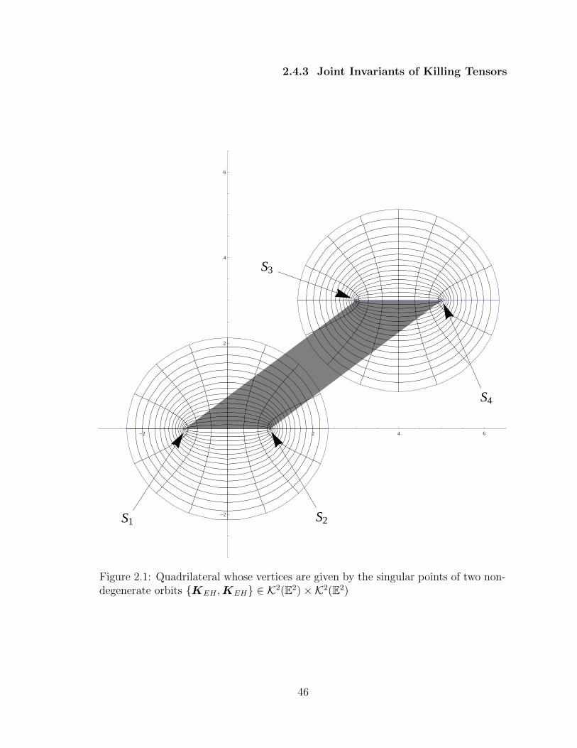
2.4.3 Joint Invariants of Killing Tensors
S3
S4
S2S1
-2 2 4 6
-2
2
4
6
Figure 2.1: Quadrilateral whose vertices are given by the singular points of two non-degenerate orbits {KEH ,KEH} ∈ K2(E2)×K2(E2)
46

Chapter 3
Superintegrable Systems on the
Euclidean Plane
We recall the significance of the first integrals of motion for a Hamiltonian system.
These are smooth functions in the generalised canonical coordinates that remain
constant along the Hamiltonian flow, or orbits, of a system. As such, they can be
identified as constants of motion for a system which elicits many familiar examples of
first integrals. Indeed, the total energy, angular momentum, and linear momentum
are all examples of constants of motion that provide physical insight about a Hamil-
tonian system: in particular, each of these is an example of a conserved quantity
that corresponds to a symmetry of the Lagrangian. A systematic way of deriving
these quantities from symmetry considerations is the heart of Noether’s theorem (see
e.g. [23]) where, for instance, conservation of energy is an artifact of the Lagrangian
being invariant under changes in time. In brief, we see that the first integrals of
motion help to establish physical properties of a Hamiltonian system by signifying
the existence of structure and symmetry.
3.1 Development of Superintegrable Systems
A Hamiltonian system with n degrees of freedom is said to be completely integrable
if it admits n globally defined, functionally independent first integrals of motion in
47
3.1 Development of Superintegrable Systems
involution with respect to the Poisson bracket (see Section 1). In the case that
such a system admits n + 1 such first integrals of motion the system is said to be
minimally superintegrable, whereas it is termed to be maximally superintegrable if it
admits 2n − 1 such first integrals. In some cases we find that a system is solvable
via orthogonal separation of variables in more than one system of coordinates, which
qualifies such systems as being multi-separable. For the purpose of this study, we
focus on superintegrable systems that exhibit this property of being multi-separable.
As discussed in Section 1.2, we can study the first integrals of natural Hamiltonian
systems
H(qi, pi) = 12gijpipj + V (qi), (3.1)
defined on flat pseudo-Riemannian manifolds which take a form quadratic in the
momenta according to
F (qi, pi) = 12Kij(qi)pipj + U(qi), i, j = 1, 2, (3.2)
which will afford orthogonal separation of variables in the associated Hamilton-Jacobi
equation in the case that Kij is a characteristic Killing two-tensor satisfying the
compatibility condition
d(KdV
)= 0. (3.3)
This is the content of Benenti’s theorem (see Section 2.3).
We can generalise this development to the study of first integrals polynomial in
the momenta of degree p upon considering Killing tensors of valence p (for a recent
account, see e.g. [28])1. Indeed, the search for first integrals of motion in higher
degrees of the momenta has been extensively studied for over a century, with Drach
initiating the study of first integrals cubic in the momenta in 1908 [19, 52]. In 2002,
Gravel and Winternitz considered superintegrable systems on E2 characterised by
one linear and one (non-trivial) cubic first integral [25]. This work was continued
by Gravel who then characterised systems with one quadratic first integral (derived
from the system admitting separability in Cartesian coordinates), and one cubic first
1Though, in studying Killing tensors of valence p > 2, we lose the interpretation of a systembeing orthogonally separable.
48

3.1 Development of Superintegrable Systems
integral [24]. The origins of the invariant theory approach can be traced back to
Winternitz and Fris in 1965 [70], in which the authors computed the invariants of
second-order symmetries of the Laplace equation defined on E2 under the action of the
isometry group, and then used these invariants to classify the orthogonal separable
webs on E2. In 2002, this geometric approach resurfaced with McLenaghan et al. in
[44], who presented it in the language of the invariant theory of Killing tensors.
In 2008, Adlam et al. [3] extended the theory constructed in [45] and derived an
invariant characterisation of the superintegrable potential admitted by the Kepler
problem through the use of invariants and joint invariants of Killing two tensors that
determined first integrals according to (3.2).
In this thesis, we continue the work of classifying superintegrable potentials on
the Euclidean plane by providing a new perspective on the ideas developed in [3].
In particular, we investigate the joint invariants of a degenerate and non-degenerate
orbit of the orbit space (K2(E2)×K2(E2))/SE(2) admitted by a Killing tensor whose
eigenvalues generate an elliptic-hyperbolic web in the canonical position, and a sec-
ond Killing tensor whose eigenvalues generate a polar web in the non-canonical po-
sition. To this end we begin by providing a joint invariant characterisation of the
Smorodinsky-Winternitz system,
H = 12
(p2x + p2
y
)− ω2
(x2 + y2
)+α
x2+β
y2, (3.4)
where α, β, and ω are arbitrary parameters. Our goal is to use joint invariants
of Killing two tensors K defined on E2 [56] to provide a link between the arbitrary
parameters of the SW potential and the parameters which characterise the associated
vector space of Killing tensors K2(E2).
Further, this will provide motivation for studying an interesting integrable per-
turbation of the SW potential that has recently appeared in the literature known
as the Tremblay-Turbiner-Winternitz (TTW) potential. Our interest will be in de-
termining which potentials admitted by the TTW system remain multi-separable in
the Euclidean plane. We remark that the results of the next two sections have been
submitted for publication (see [57]).
49

3.2 Characterisation of the Smorodinsky-Winternitz Potential
3.2 Characterisation of the Smorodinsky-Winternitz
Potential
The superintegrability of the Smorodinsky-Winternitz (SW) potential is a simple con-
sequence of its multi-separability with respect to both canonical polar and canonical
Cartesian coordinates. The property of the coordinate web being canonical can be
interpreted either geometrically, (see Figure 1.1), or with respect to the form of the
general characteristic Killing tensor defining the orthogonal coordinate web (see [45]).
Geometrically, canonical Cartesian coordinates are aligned with the coordinate axes
and canonical polar coordinates have their singular point coincide with the origin of
the coordinate axes; the associated Killing tensors for each canonical web respectively
take the forms (3.6) and (3.8) given below.
Since the SW potential is of the form V = f(x)+g(y), it immediately follows that
the system enjoys separability with respect to (canonical) Cartesian coordinates, and
so the Hamiltonian flow defined with respect to (3.4) admits a first integral quadratic
in the momenta according to
F1 = 12Kij
1 pipj + U1, i, j = 1, 2, (3.5)
where Kij1 is the Killing two-tensor whose normal eigenvectors generate the (canoni-
cal) Cartesian coordinate web:
Kij1 =
(1 0
0 0
). (3.6)
Imposing the compatibility condition (3.3) requires that dU1 = K1dV, which we can
readily integrate to obtain that U1(x, y) = αx2− ω2x2. This provides us with the first
non-trivial quadratic first integral.
If we transform the potential of (3.4) to polar coordinates we immediately see that
it is of the from V (r, θ) = f(θ)r2
+ g(r), and so that indeed the Hamiltonian system
defined by (3.4) is also separable with respect to (canonical) polar coordinates. Thus,
50

3.2 Characterisation of the Smorodinsky-Winternitz Potential
we have that it admits a second quadratic first integral according to
F ij2 = 1
2Kij
2 pipj + U2, i, j = 1, 2, (3.7)
where Kij2 is given by the Killing two-tensor whose normal eigenvectors generate the
(canonical) polar web:
Kij2 =
(y2 −xy−xy x2
)(3.8)
In this case, we find upon integrating dU2 = K2dV that U2(x, y) = ay2
x2+ bx2
y2, and so
we have obtained two non-trivial quadratic first integrals.
The functional independence of F1 and F2 follows from considering that the wedge
product of their differentials with dH at a point p ∈ E2 is non-vanishing
dH ∧ dF1 ∧ dF2(p) 6= 0,
a criterion which yields that the set of F1 and F2 defines a coordinate system, since
this is equivalent to saying that the Jacobian determinant of the functions F1 and
F2 at a point p ∈ M is non-vanishing, and so by the Implicit Function theorem
the set indeed forms a coordinate system (e.g. see [40]). Furthermore, since both
are mutually in involution with the Hamiltonian, i.e. {F1, H} = {F2, H} = 0, then
we have at once that the Hamiltonian system (3.4) is superintegrable (since it is
multi-separable) with 2n − 1 = 3 functionally independent first integrals of motion,
namely the set {H,F1, F2}. Since the function F3 = F1 + F2 is also a first integral
of motion, with an associated Killing two-tensor K1 + K2 = KEH , where KEH
denotes the (canonical) Killing tensor whose normal eigenvectors generate the elliptic-
hyperbolic coordinate web, then it follows that the SW potential will also be separable
in (canonical) elliptic-hyperbolic coordinates. Indeed, the canonical characteristic
Killing tensor that generates the elliptic-hyperbolic coordinate web is given by
KijEH =
(y2 + k2 −xy−xy x2
), (3.9)
(where k2 is an invariant to be defined below) which makes it clear that any potential
51

3.2 Characterisation of the Smorodinsky-Winternitz Potential
of a Hamiltonian system compatible with both the valence two Killing tensor of polar
type and the valence two Killing tensor of Cartesian type will also be compatible with
the valence two Killing tensor of elliptic-hyperbolic type, by linearity of the exterior
derivative.
We can now make use of joint invariants, introduced in Section 2.4.3, to conclude
that separation in (canonical) polar and (canonical) elliptic-hyperbolic coordinates
implies that the quadrilateral (see Figure 2.1) S1S2S4S3 degenerates in the following
manner. Denote by S1 and S2 the singular points of the Killing two-tensor K3 whose
first integral is given by F3 as defined above (i.e. K3 = KEH), and similarly, take S3
and S4 as the singular points of K2. Then since both K1 and K2, and hence K3
are in canonical form, we find that the quadrilateral S1S2S4S3 degenerates according
to the invariant conditions S3 = S4, and dist(S1, S3) = dist(S2, S4). In terms of the
fundamental joint invariants (2.61), we can equivalently write these conditions as
∆′3 = 0, ∆′8 = ∆′9,
respectively.
Conversely, if we begin with a general potential V of a natural Hamiltonian
(3.1) and impose that the Hamiltonian system be multi-separable with respect to
canonical polar and canonical Cartesian coordinates, i.e. impose that it admits two
quadratic first integrals given by F1 and F2 as above, then integrating the condi-
tions dUi = KidV for i = 1, 2 will yield the Smorodinsky-Winternitz potential,
which follows from [22, 1]. Therefore, we can conclude that the superintegrable
system given by the Smorodinsky-Winternitz potential is characterised by a pair
of Killing tensors (K2,K3) ∈ K2(E2) × K2(E2) whose position in the orbit space
(K2(E2)×K2(E2))/SE(2) is determined by the invariant conditions
∆′1 6= 0, ∆′3 = 0, ∆′4 6= 0, ∆′6 6= 0, ∆′7 = ∆′8 = ∆′9.
Thus, we have the following:
52
3.2.1 Weakening the Conditions
Theorem 3.10. Let V be the potential of a natural Hamiltonian
H(qi, pi) = 12gij(qi)pipj + V (qi), i, j = 1, 2
satisfying d(K`dV
)= 0, ` = 2, 3 for a pair of Killing tensors (K2,K3) ∈ K2(E2)×
K2(E2). Then the following statements are equivalent:
(1) The pair (K2,K3) ∈ K2(E2)×K2(E2) is invariantly characterised by the con-
ditions
∆′1 6= 0, ∆′3 = 0, ∆′4 6= 0,
∆′6 6= 0, ∆′7 = ∆′8 = ∆′9. (3.11)
(2) The potential V given by the natural Hamiltonian is the Smorodinsky-Winternitz
potential given in Cartesian coordinates (q1, q2) = (x, y) by
V (x, y) = −ω2(x2 + y2) +α
x2+β
y2. (3.12)
Thus, we have shown that by invariantly characterising the pair (K2,K3) ∈K2(E2)×K2(E2), we have in fact characterised the SW potential which they define.
Next, we study what happens to the form of the SW potential in the case that we
weaken the invariant conditions (3.11).
3.2.1 Weakening the Conditions
We shall first suppose that the Hamiltonian system (3.1) admits two quadratic first
integrals of motion according to (3.5) and (3.7). Further, suppose that the Killing
tensor KP generates (non-canonical) polar coordinates, and that the Killing tensor
KEH generates (non-canonical) elliptic-hyperbolic coordinates. Without loss of gen-
erality, and to facilitate calculations, we will assume that KEH is in the canonical
form, so that the elliptic-hyperbolic web is generated in the canonical position. Then
the singular points of the two webs form a general triangle 4S1S2S3— see Figure
3.1. Considering the fundamental joint invariants (2.61), this arrangement induces
53

3.2.1 Weakening the Conditions
S3
S2S1
-2 2 4 6
-2
2
4
6
Figure 3.1: Triangle whose vertices are given by the singular points of two Killing ten-sors, one non-degenerate and the other degenerate, (KEH ,KP ) ∈ K2(E2)×K2(E2).In this case, KEH is in the canonical form.
the following invariant conditions for the pair (KP ,KEH) ∈ K2(E2)×K2(E2):
∆′1 6= 0,∆′3 = 0,∆′4 6= 0,
∆′6 6= 0,∆′7 = ∆′9 6= ∆′8. (3.13)
We then have the following components for the respective Killing tensors as follows
[45]
KijP =
((y − b)2 (x− a)(y − b)
(x− a)(y − b) (x− a)2
), a, b ∈ R, (3.14)
54
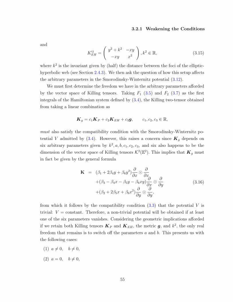
3.2.1 Weakening the Conditions
and
KijEH =
(y2 + k2 −xy−xy x2
), k2 ∈ R, (3.15)
where k2 is the invariant given by (half) the distance between the foci of the elliptic-
hyperbolic web (see Section 2.4.3). We then ask the question of how this setup affects
the arbitrary parameters in the Smorodinsky-Winternitz potential (3.12).
We must first determine the freedom we have in the arbitrary parameters afforded
by the vector space of Killing tensors. Taking F1 (3.5) and F2 (3.7) as the first
integrals of the Hamiltonian system defined by (3.4), the Killing two-tensor obtained
from taking a linear combination as
Kg = c1KP + c2KEH + c3g, c1, c2, c3 ∈ R,
must also satisfy the compatibility condition with the Smorodinsky-Winternitz po-
tential V admitted by (3.4). However, this raises a concern since Kg depends on
six arbitrary parameters given by k2, a, b, c1, c2, c3, and six also happens to be the
dimension of the vector space of Killing tensors K2(E2). This implies that Kg must
in fact be given by the general formula
K = (β1 + 2β4y + β6y2)∂
∂x� ∂
∂x
+(β3 − β4x− β5y − β6xy)∂
∂x� ∂
∂y
+(β2 + 2β5x+ β6x2)∂
∂y� ∂
∂y,
(3.16)
from which it follows by the compatibility condition (3.3) that the potential V is
trivial: V = constant. Therefore, a non-trivial potential will be obtained if at least
one of the six parameters vanishes. Considering the geometric implications afforded
if we retain both Killing tensors KP and KEH , the metric g, and k2, the only real
freedom that remains is to switch off the parameters a and b. This presents us with
the following cases:
(1) a 6= 0, b 6= 0,
(2) a = 0, b 6= 0,
55

3.2.1 Weakening the Conditions
(3) a 6= 0, b = 0,
(4) a = b = 0.
The first case imposed that the SW potential would assume a trivial form. We
can introduce a new fundamental invariant (replacing ∆′9 in (2.61), since with respect
to the two orthogonal coordinate webs ∆′9 = ∆′7) given by the area of 4S1S2S3. In
terms of the fundamental joint invariants (2.61) and the area of 4S1S2S3, we then
have the following invariant characterisation.
(1) ∆′1 6= 0,∆′3 = 0,∆′4 6= 0,∆′6 6= 0,∆′7 6= 0,∆′8 6= 0, the area of 4S1S2S3 6= 0.
(2) ∆′1 6= 0,∆′3 = 0,∆′4 6= 0,∆′6 6= 0,∆′7 − ∆′8 = 0, the area of 4S1S2S3 6= 0. In
this case the 4S1S2S3 takes the form of an isosceles triangle.
(3) ∆′1 6= 0,∆′3 = 0,∆′4 6= 0,∆′6 6= 0,∆′7 6= ∆′8, the area of 4S1S2S3 = 0. We
remark that this is the case when the singular points all lie on the x−axis.
(4) ∆′1 6= 0,∆′3 = 0,∆′4 6= 0,∆′6 6= 0,∆′7 = ∆′8, area of 4S1S2S3 = 0
We can next characterise the arbitrary parameters a and b as joint invariants
themselves by writing them in terms of the fundamental joint invariants (2.61). To
this end, we consider the general Killing tensor whose components with respect to
Cartesian coordinates (q1, q2) are given by (3.16) and suppose that β6 6= 0,∆ = 0,
where
∆ = (β24 − β2
5 + β6(β2 − β1))2 + 4(β6β3 + β4β5)2.
If we consider the Killing tensor KP , we can compare it with (3.16) via
Kij = `gij +mKPij , (3.17)
where KPij = gikg`jK
k`P , with Kk`
P given by (3.14). Comparing components on both
sides of (3.17) then amounts to identifying
α1 + 2α4y + α6y2 = `+m(y − b)2,
α3 − α4x− α5y − α6xy = −m(x− a)(y − b),
α2 + 2α5x+ α6x2 = `+m(x− a)2,
56

3.2.1 Weakening the Conditions
which admits the following identification
(a, b) =
(−α5
α6
,−α4
α6
).
Through a bit of algebraic manipulation, we can then obtain an expression for each
parameter in terms of the joint invariants (2.61):
a =(∆′4)2(∆′8 −∆′7)− 1
2∆′6
2∆′4√
∆′6
and
b =
√√√√∆′7 −
(a−
√∆′6
2∆′4
)2
.
Solving the PDEs that come from imposing the compatibility condition (3.3) for the
Killing two-tensor defined by (3.14) and the SW potential (3.12), we arrive at the
following equation
ω2(bx− ay) +a(b− y)α
x4+b(−a+ x)β
y4= 0, (3.18)
which puts into evidence the following relationship
(1) a 6= 0, b 6= 0 yields the trivial potential V = 0,
(2) a = 0, b 6= 0 yields the potential V =β
y2,
(3) a 6= 0, b = 0 yields the potential V =α
x2,
(4) a = 0, b = 0 yields the general Smorodinsky-Winternitz potential (3.12).
Henceforth, we arrive at the conclusion that the more geometric structure the pair
(KP ,KEH) ∈ K2(E2)×K2(E2) has (in the sense of placing the polar coordinate web
in restricted positions), the more general the Smorodinsky-Winternitz potential (3.12)
becomes. In each of the cases described above the corresponding pair (KP ,KEH) ∈K2(E2)×K2(E2) belongs to a different orbit of the group action SE(2) � K2(E2)×
57

3.3 The Tremblay-Turbiner-Winternitz System
K2(E2) (see Section 2.4.2, eq. 2.49). In fact, our above analysis shows that these
corresponding orbits have been explicitly distinguished by means of joint invariants
(2.61) of the action (2.49). Considering our work as an extension of the results
obtained in [3], we see that we have demonstrated that the use of joint invariants
to classify the orbits of (K2(E2) × K2(E2))/SE(2) leads to a classification of the
corresponding superintegrable potentials defined by quadratic first integrals in E2.
We remark on the further development of this perspective in Chapter 4.
3.3 The Tremblay-Turbiner-Winternitz System
We now consider the Tremblay-Turbiner-Winternitz (TTW) potential introduced in
2009 [65]. It is defined in polar coordinates by the natural Hamiltonian
H = p2r +
1
rpr +
1
r2p2θ − ω2r2 +
1
r2
(λ1
cos2 kθ+
λ2
sin2 kθ
), (3.19)
which demonstrates that its potential,
V (r, θ) = −ω2r2 +1
r2
(λ1
cos2 kθ+
λ2
sin2 kθ
), (3.20)
is of the from V (r, θ) = f(θ)r2
+g(r) and so is separable in (canonical) polar coordinates.
By the results of Section 2.3, we have that the system admits a first integral of motion
taking the form
F (qi, pi) = 12Kij(qi)pipj + U(qi), i, j = 1, 2,
where Kij is the Killing two-tensor which generates (canonical) polar coordinates,
i.e. (3.8) and U is determined via dU = KdV . We then seek to answer the following
question posed in the introduction of this thesis:
For which values of k is the TTW system multi-separable?
In other words, we seek to determine for which values of k the TTW potential (3.20)
admits an additional (non-trivial) functionally independent quadratic first integral of
58

3.3 The Tremblay-Turbiner-Winternitz System
motion.
To allow for arbitrary k ∈ R, we cannot transform the TTW system back into
Cartesian coordinates. Indeed, such a transformation would require the use of trigono-
metric identities in cos kθ and sin kθ, which require k to in general be an integer.
Thus we must carry out all our calculations in polar coordinates. To this end we
shall first rewrite the formula defining a general Killing tensor Kg ∈ K2(E2) in polar
coordinates.
On this note, we make use of the result that on a manifoldM of constant curva-
ture, generalised Killing tensors are formed as sums of symmetrised tensor products
of generalised Killing vectors on M (see [18]). This means that on E2, we have
Kg = AijX i �Xj +BiX i �R+ CR�R, i, j = 1, 2, (3.21)
for some tensor Aij, vector Bi and constant C. If we take as our basis of Killing
vectors on E2
X1 = cos θ∂
∂r− sin θ
r
∂
∂θ,
X2 = sin θ∂
∂r+
cos θ
r
∂
∂θ, (3.22)
R =∂
∂θ,
and let (Aij)
=
(β1 β3
β3 β2
), Bi = (β4, β5), C = β6, (3.23)
then we find upon substituting (3.22) and (3.23) into (3.21) and taking the symmetric
tensor products then
K p = AijX i �Xj +BiX i �R+ CR�R
59

3.3 The Tremblay-Turbiner-Winternitz System
and we derive that the components of the general Killing tensor Kp ∈ K2(E2) defined
with respect to polar coordinates are given by
K11p = 2β3 cos θ sin θ + β1 cos2 θ + β2 sin2 θ,
K12p = 2β4 cos θ + 2β5 sin θ +
2β3 cos 2θ
r− 2β1 cos θ sin θ
r+
2β2 cos θ sin θ
r, (3.24)
K22p = β6 −
2β3 cos θ sin θ
r2+β1 sin2 θ
r2+β2 cos2 θ
r2− 2β4 sin θ
r+
2β5 cos θ
r.
Substituting K p and the potential (3.20) into the compatibility condition,
d(K pdV
)= 0, (3.25)
we arrive at a complicated trigonometric equation in terms of the arbitrary parame-
ters k, λ1, λ2, βi, i = 1, . . . 6 (see eq. (C.1) in Appendix C). To solve this equation, we
expand it over the following set M of trigonometric functions
M ={1, cos(θ), sin(θ), cos(2θ), sin(2θ),
cos((1 + k)θ), sin((1 + k)θ), cos((1− k)θ), sin((1− k)θ),
cos((1 + 2k)θ), sin((1 + 2k)θ), cos((1− 2k)θ), sin((1− 2k)θ),
cos((1 + 3k)θ), sin((1 + 3k)θ), cos((1 + 3k)θ), sin((1 + 3k)θ),
cos(2(1 + k)θ), sin(2(1 + k)θ), cos(2(1− k)θ), sin(2(1− k)θ),
cos(2(1 + 2k)θ), sin(2(1 + 2k)θ), cos(2(1− 2k)θ), sin(2(1− 2k)θ),
cos(2(1 + 3k)θ), sin(2(1 + 3k)θ), cos(2(1 + 3k)θ), sin(2(1 + 3k)θ)}, (3.26)
which is the set obtained by expanding the trigonometric functions in (C.1), ignoring
any trig identities. The set M is linearly dependent when the arguments of the
trigonometric functions coincide (see Appendix D), a property which depends on the
values assumed by the parameter k. By plotting the arguments as functions over k
and determining the intersection points of these functions, we thus determine that
60

3.3 The Tremblay-Turbiner-Winternitz System
the set (3.26) is linearly dependent for the following values of k:
k =± 2,±3
2,±1,±1
2,±1
4,±1
6,±1
8,± 1
10,± 1
12,± 1
14,± 1
16,±3
4,±2
3,
± 3
8,±1
3,± 3
10,±2
7,± 3
14,±1
5,± 3
16,±2
5,±1
7.
(3.27)
In the case when k does not equal one of the above values, the set M is linearly
independent and so we can set each of the coefficients to zero in the trigonometric
equations that we obtain upon the substituting (3.21) and (3.20) into (3.25) and
expanding over the set M . This argument leads to an overdetermined system of
polynomial equations which we can then solve for the variables k, βi, and λj, i =
1, . . . , 6, j = 1, 2. Before completing this computation we shall reduce the number of
polynomial equations with the following argument.
Since the TTW potential (3.20) is separable in polar coordinates then if it were
to admit another quadratic first integral of motion it would have been defined by a
Killing two-tensor which is an element of the 5-dimensional vector subspace
Ks = AijX i �Xj +BiX i �R, i, j = 1, 2,
which is the vector space (3.21) with the “polar” term factored out. Substituting
this Killing tensor Ks into the compatibility condition (3.25) for the TTW potential
(3.20), we arrive a system of equations for which it is possible to expand over the basis
L = {1, cos θ, sin θ, cos 2θ, sin 2θ}. This results in the following necessary condition
on the parameters of the Killing tensor Ks:
β24 + β2
5 = 0.
Since all parameters are assumed to be real, the above holds provided β4 = β5 = 0.
Therefore we conclude that if the potential (3.20) is separable in another orthogonal
coordinate system, other than polar, it can only be the Cartesian system of coordi-
nates. We can now repeat the same argument outlined above with a simpler Killing
tensor. Namely, the Killing two-tensor that defines Cartesian coordinates in a general
61

3.3 The Tremblay-Turbiner-Winternitz System
position [45],
KijC =
(cos2(θ − φ) −1
2r sin(2(θ − φ))
−12r sin(2(θ − φ)) r2 sin2(θ − φ)
), (3.28)
where φ denotes the angle by which the Cartesian coordinate system is rotated (recall
the Cartesian web in Figure 1.2). Substituting (3.28) and (3.20) into the compatibility
condition (3.25), we arrive at the following equation
(3.29)csc2 kθ(6k cos 2(θ − φ) cot kθ +
(4 + 2k2 − 3k2 csc2 kθ
)sin 2(θ − φ)
)λ2
+ sec2 kθ(−6k cos 2(θ − φ) tan kθ
+(4 + 2k2 − 3k2 sec2 kθ
)sin 2(θ − φ)
)λ1 = 0.
We can then expand this over a subset of N ⊂M given by
N ={1, cos(2θ), sin(2θ),
cos(2(1 + k)θ), sin(2(1 + k)θ), cos(2(1− k)θ), sin(2(1− k)θ),
cos(2(1 + 2k)θ), sin(2(1 + 2k)θ), cos(2(1− 2k)θ), sin(2(1− 2k)θ),
cos(2(1 + 3k)θ), sin(2(1 + 3k)θ), cos(2(1 + 3k)θ), sin(2(1 + 3k)θ)} (3.30)
which we determine to be linearly dependent for the following values of k
k = ±1,±2,±2/3,±1/2,±2/5, (3.31)
which are indeed a subset of the values obtained in (3.27). Expanding the equation
(3.29) over the set N , and assuming it to be linearly independent (i.e. excluding the
values of k given by (3.31)), we arrive at the following (reduced) system of polynomial
62

3.3 The Tremblay-Turbiner-Winternitz System
equations in the variables φ, k, λ1, λ2:
(−2 + k)(−1 + k) (λ1 − λ2) sin 2φ = 0,
(−2 + k(−15 + 23k)) (λ1 − λ2) sin 2φ = 0,
(−2 + k(15 + 23k)) (λ1 − λ2) sin 2φ = 0,
(1 + k)(2 + k) (λ1 − λ2) sin 2φ = 0,
(−1 + k)(−1 + 2k) (λ1 + λ2) sin 2φ = 0,
(1 + k)(1 + 2k) (λ1 + λ2) sin 2φ = 0,
(−1 + 2k)(1 + 2k) (λ1 + λ2) sin 2φ = 0,
(−2 + k)(−1 + k) (λ1 − λ2) cos 2φ = 0,
(−2 + k(−15 + 23k)) (λ1 − λ2) cos 2φ = 0,
(−2 + k(15 + 23k)) (λ1 − λ2) cos 2φ = 0,
(1 + k)(2 + k) (λ1 − λ2) cos 2φ = 0,
(−1 + k)(−1 + 2k) (λ1 + λ2) cos 2φ = 0,
(1 + k)(1 + 2k) (λ1 + λ2) cos 2φ = 0,
(−1 + 2k)(1 + 2k) (λ1 + λ2) cos 2φ = 0.
There is no non-trivial solution for which the above system is satisfied. Considering
the set of linearly dependent functions, we substitute into equation (3.29) with the
special values of k given in (3.31) to yield the following possible cases
(1) k = ±1
Imposes φ = 0.
(2) k = ±2
Imposes {λ1 = 0, φ = nπ/2} or, {λ2 = 0, φ = nπ/4}, n ∈ N.
(3) k = ±2/3,±1/2,±2/5,
Imposes λ1 = λ2 = 0.
63

3.3 The Tremblay-Turbiner-Winternitz System
Thus, we conclude that k = ±1 are the only values of k for which the full TTW
potential (3.20) admits two quadratic first integrals of motion. For these values of k,
the TTW system reduces to the Smorodinsky-Winternitz system discussed in Section
3.2. Hence, we have proven the following
Proposition 3.32. The general TTW potential given by (3.20) is a multi-separable
superintegrable potential only when k = ±1.
The case k = ±2 yields the well-known Calogero system on the line (see e.g. [10,
14]). The conclusion of our above argument is that only when either λ1 or λ2 vanishes
does this potential admit separation in general Cartesian coordinates according to a
non-canonical Killing tensorKC whose components are given by (3.28). In particular,
the compatibility condition d(KCdV ) = 0 will be satisfied for the potential
V (r, θ) = −ω2r2 +λ1
cos 2θ+
λ2
sin 2θ
when either λ1 = 0 and φ = nπ/2, or λ2 = 0, and φ = nπ/4.
Our results demonstrate that this approach to defining an infinite family of su-
perintegrable systems appears to destroy the geometry of the associated orbit space
(K2(E2) × K2(E2))/SE(2). In other words, it seems unlikely for systems defined in
this manner to admit two quadratic first integrals of motion for multiple values of
the introduced parameter. In 2010 [50], this method was utilised by Post and Win-
ternitz to construct another infinite family of superintegrable systems dependent on
a parameter k, namely a potential that appeared as a second-order perturbation of
the Kepler-Coulomb potential. They then established an equivalence between this
new system and the TTW system through a Stackel transform, which maps Hamil-
tonians to Hamiltonians, and hence developed a direct relation between the integrals
of motion and trajectories of each system. Indeed, it would be of interest to pursue
this equivalence through the invariant theory of Killing tensors which could possibly
facilitate the search for these Stackel equivalent systems on a manifold.
64
Chapter 4
Conclusions and Outlook
We have invariantly characterised the Smorodinsky-Winternitz superintegrable po-
tential modulo the action of the isometry group SE(2) in terms of joint invariants
of the associated Killing tensors by taking them as points in the product space
K2(E2)×K2(E2). We can extend this result to the problem of classification of arbi-
trary superintegrable potentials defined in spaces of constant curvature by classifying
first any associated Killing tensors that define first integrals of motion for the class
of superintegrable systems in question (e.g., superintegrable systems that admit only
quadratic first integrals of motion). These Killing tensors are identified as elements of
the corresponding product spaces, whose factors are the corresponding vector spaces
of Killing tensors representing the associated orbits in the induced orbit space under
the action of the isometry group in such product spaces.
Additionally, we have proven that the general TTW potential is a superintegrable
system with two functionally independent quadratic first integrals of motion only for
k = ±1, that is when it reduces to the Smorodinsky-Winternitz potential. If we
allow one of the arbitrary parameters in the TTW potential to vanish, then a second
multi-separable system is obtained when k = ±2. Therefore we have established that
the general superintegrability of the TTW system for other k values must come from
a (non-trivial) higher order (i.e. not quadratic) first integral.
The results contained within this thesis motivate the complete classification of
Hamiltonian systems with two degrees of freedom, which are superintegrable in the
sense of being multi-separable. The introduction of an additional arbitrary parameter
65

4 Conclusions and Outlook
into a superintegrable potential appears to be very destructive, in the sense that it
destroys the property of multi-separability for all but one choice of the arbitrary
parameter. This hints towards a characterisation on the Euclidean plane for all
superintegrable systems obtained as perturbations of known superintegrable systems,
and further, the classification of all multi-separable superintegrable systems defined
on the Euclidean plane.
Furthermore, we can extend our results to studying superintegrable systems de-
fined on different two-dimensional spaces, such as on the Minkowski plane or the
2D sphere. In the case of the former, the study becomes complicated by the fact
that there are nine orthogonal coordinate webs and instead of a discrete set of singu-
lar points, there are singular regions admitted by complex-valued eigenvalues of the
associated characteristic Killing tensor. In the case of the 2D sphere, the study is
simplified as a result of both the additional symmetry of the manifold and its com-
pactness. Indeed, there are instead only two orthogonal coordinate webs defined on
the sphere, and the set of singular points remains discrete. It is of immediate interest
to the author to carry out the classification of all multi-separable systems defined on
spaces of constant curvature with two degrees of freedom.
66

Bibliography
[1] C. M. Adlam, A Lie Group Theory Approach to the Problem of Classification
of Superintegrable Potentials in the Euclidean Plane, Ph.D. thesis, Dalhousie
University, 2005. ↑ 2, 8, 38, 52
[2] C. M. Adlam, R. G. McLenaghan, and R. G. Smirnov, An orbit analysis approach
to the study of superintegrable systems in the Euclidean plane, Physics of Atomic
Nuclei 70 (2007), 486–490. ↑ 8
[3] , On geometric properties of joint invariants of Killing tensors, Symme-
tries and Overdetermined Systems of Partial Differential Equations, IMA Vol.
Math. Appl., vol. 144, Springer, New York, 2008, pp. 205–221. ↑ 2, 5, 32, 38,
42, 45, 49, 58
[4] V. I. Arnol′d, Mathematical Methods of Classical Mechanics, Graduate Texts
in Mathematics, vol. 60, Springer-Verlag, New York, 1989, Translated from the
1974 Russian original by K. Vogtmann and A. Weinstein, Corrected reprint of
the second (1989) edition. ↑ 23, 24, 27
[5] S. Benenti, Intrinsic characterization of the variable separation in the Hamilton-
Jacobi equation, J. Math. Phys. 38 (1997), no. 12, 6578–6602. ↑ 31, 38, 44
[6] J. Bertrand, Memoire sur quelques-unes des formes les plus simples que puissent
presenter les integrales des equations differentielles du mouvement d’un point
materiel, (1857), no. 2, 113. ↑ 29
67

Bibliography
[7] , Theoreme relatif au mouvement d’un point attire vers un centre fixe,
Comptes Rendus des Seances de l’Academie des Sciences (1857), no. 76, 909. ↑3
[8] A. Bruce, R. McLenaghan, and R. Smirnov, Benenti’s theorem and the method
of moving frames, Reports on Mathematical Physics 48 (2001), no. 1, 227–234.
↑ 32
[9] , A geometrical approach to the problem of integrability of hamiltonian
systems by separation of variables, Journal of Geometry and Physics 39 (2001),
no. 4, 301–322. ↑ 32
[10] F. Calogero, General solution of a three-body problem in the plane, J. Phys. A
36, no. 26, 7291–7299. ↑ 64
[11] E. Cartan, Lecons sur la geometrie projective complexe. La theorie des groupes
finis et continus et la geometrie differentielle traitees par la methode du repere
mobile. Lecons sur la theorie des espaces a connexion projective, Les Grands
Classiques Gauthier-Villars. [Gauthier-Villars Great Classics], Editions Jacques
Gabay (French), Reprint of the editions of 1931, 1937 and 1937. ↑ 38
[12] M. Chanachowicz, C. M. Chanu, and R. G. McLenaghan, r-separation of vari-
ables for the conformally invariant Laplace-Beltrami equation, J. Geom. Phys.
59, no. 7, 876–884. ↑ 2, 38
[13] C. Chanu, L. Degiovanni, and R. G. McLenaghan, Geometrical classification
of Killing tensors on bidimensional flat manifolds, J. Math. Phys. 47, no. 7,
073506, 20. ↑ 2, 38
[14] C. Chanu, L. Degiovanni, and G. Rastelli, Superintegrable three-body systems on
the line, J. Math. Phys. 49, no. 11, 112901, 10. ↑ 64
[15] C. Cochran, The equivalence problem for orthogonally separable webs on spaces
of constant curvature, Dissertation, Dalhousie University, 2011. ↑ 2, 38
[16] G. Darboux, Sur un probleme de mecanique, Arch. Neerlandaises Sci 6 (1901),
371–376. ↑ 29
68

Bibliography
[17] R. J. Deeley, J. T. Horwood, R. G. McLenaghan, and R. G. Smirnov, Theory of
algebraic invariants of vector spaces of Killing tensors: methods for computing
the fundamental invariants, pp. 1079–1086. ↑ 2, 38
[18] R. Delong, Killing tensors and the Hamilton-Jacobi equation, Dissertation, Uni-
versity of Minnesota, 1982. ↑ 33, 34, 59
[19] J. Drach, Sur le probleme logique de l’integration des equations differentielles,
Ann. Fac. Sci. Toulouse Sci. Math. Sci. Phys. (2) 10, 393–472 (French). ↑ 48
[20] L. Eisenhart, Separable systems of Stackel, The Annals of Mathematics 35
(1934), no. 2, 284–305. ↑ 30, 38
[21] N. Evans, Superintegrability in classical mechanics, Physical Review A 41 (1990),
no. 10, 5666. ↑ 3, 8
[22] J. Fris, V. Mandrosov, Y. A. Smorodinsky, M. Uhlır, and P. Winternitz, On
higher symmetries in quantum mechanics, Phys. Lett. 16 (1965), 354–356. ↑ 7,
8, 52
[23] H. Goldstein, Classical Mechanics, 2 ed., Addison-Wesley Publishing Co., Read-
ing, Mass., Addison-Wesley Series in Physics. ↑ 47
[24] S. Gravel, Hamiltonians separable in Cartesian coordinates and third-order in-
tegrals of motion, J. Math. Phys. 45, no. 3, 1003–1019. ↑ 49
[25] S. Gravel and P. Winternitz, Superintegrability with third-order integrals in quan-
tum and classical mechanics, J. Math. Phys. 43 (2002), no. 12, 5902–5912. ↑48
[26] J. Harnad and O. Yermolayeva, Superintegrability, Lax matrices and separation
of variables, 65–73. ↑ 6
[27] T. Hawkins, Emergence of the theory of Lie groups, Sources and Studies in the
History of Mathematics and Physical Sciences, Springer-Verlag, New York, 2000,
An essay in the history of mathematics 1869–1926. ↑ 32
69

Bibliography
[28] J. T. Horwood, Higher order first integrals in classical mechanics, Journal of
Mathematical Physics 48 (2007), 102902. ↑ 48
[29] , Invariant theory of Killing tensors, Dissertation, University of Cam-
bridge, 2008. ↑ 2, 38, 75, 77
[30] , On the theory of algebraic invariants of vector spaces of Killing tensors,
vol. 58, Elsevier, 2008, pp. 487–501. ↑ 2, 38
[31] J. T. Horwood, R. G. McLenaghan, and R. G. Smirnov, Invariant classification
of orthogonally separable Hamiltonian systems in Euclidean space, Communica-
tions in mathematical physics 259 (2005), no. 3, 679–709. ↑ 2, 8, 38
[32] , Hamilton-Jacobi theory in three-dimensional Minkowski space via Car-
tan geometry, J. Math. Phys. 50 (2009), no. 5, 053507, 41. ↑ 2, 38
[33] E. G. Kalnins, J. M. Kress, and W. Miller, Jr., Families of classical subgroup
separable superintegrable systems, J. Phys. A 43 (2010), no. 9, 092001, 8. ↑ 2
[34] , Tools for verifying classical and quantum superintegrability, SIGMA
Symmetry Integrability Geom. Methods Appl. 6 (2010), Paper 066, 23. ↑ 4
[35] , A recurrence relation approach to higher order quantum superintegra-
bility, SIGMA 7 (2011), no. 031, 24. ↑ 2, 4
[36] , Structure relations for the symmetry algebras of quantum superintegrable
systems, Journal of Physics: Conference Series 343 (2012), no. 1, 012075. ↑ 2, 4
[37] E. G. Kalnins, J. M. Kress, and G. S. Pogosyan, Superintegrability and higher-
order constants for classical and quantum systems, Physics of Atomic Nuclei 74
(2011), 914–918. ↑ 2, 4
[38] I. A. Kogan, Two algorithms for a moving frame construction, Canad. J. Math.
55 (2003), no. 2, 266–291. ↑ 38, 40
[39] L. D. Landau and E. M. Lifshitz, Mechanics, Course of Theoretical Physics, Vol.
1. Translated from the Russian by J. B. Bell, Pergamon Press. ↑ 19, 24, 25
70

Bibliography
[40] J. M. Lee, Introduction to Smooth Manifolds, Grad. Texts in Math., vol. 218,
Springer-Verlag, New York, 2003. ↑ 11, 13, 14, 16, 17, 20, 51
[41] T. Levi-Civita, Sulla integrazione della equazione di Hamilton-Jacobi per sepa-
razione di variabili, Mathematische Annalen 59 (1904), no. 3, 383–397. ↑ 27
[42] J. Liouville, Sur quelques cas particuliers o les quations de mouvement dun point
matriel peuvent sintegrer, Journ. Math. Pure and Appl 11 (1846), 345–378. ↑ 4,
28
[43] A. Makarov, Y. A. Smorodinsky, K. Valiev, and P. Winternitz, A systematic
search for nonrelativistic systems with dynamical symmetries, Il Nuovo Cimento
A (1965-1970) 52 (1967), 1061–1084. ↑ 8
[44] R. G. McLenaghan, R. G. Smirnov, and D. The, Towards a classification of cubic
integrals of motion, pp. 199–209. ↑ 49
[45] , Group invariant classification of separable Hamiltonian systems in the
Euclidean plane and the O(4)-symmetric Yang-Mills theories of Yatsun, J. Math.
Phys. 43 (2002), no. 3, 1422–1440. ↑ 2, 38, 39, 41, 42, 45, 49, 50, 54, 62
[46] A. S. Miscenko and A. T. Fomenko, A generalized Liouville method for the inte-
gration of Hamiltonian systems, Funkcional. Anal. i Prilozen. 12, no. 2, 46–56,
96 (Russian). ↑ 3
[47] G. Morera, Sulla separazione delle variabili nelle equazioni del moto di un punto
materiale su una superfice, Atti. Sci. di Torino 16 (1881), 276–295. ↑ 28
[48] N. N. Nehorosev, Action-angle variables, and their generalizations, Trudy
Moskov. Mat. Obsc. 26, 181–198 (Russian). ↑ 3
[49] P. J. Olver, Classical Invariant Theory, London Mathematical Society Student
Texts, vol. 44, Cambridge University Press. ↑ 34, 38, 39, 44
[50] S. Post and P. Winternitz, An infinite family of superintegrable deformations of
the Coulomb potential, J. Phys. A 43, no. 22, 222001, 11. ↑ 64
71
Bibliography
[51] M. F. Ranada, On a second Lax structure for the Calogero-Moser system: time-
dependent constants and superintegrability, Phys. Lett. A 277, no. 4-5, 219–222.
↑ 6
[52] , Superintegrable n = 2 systems, quadratic constants of motion, and po-
tentials of Drach, Journal of Mathematical Physics 38 (1997), 4165. ↑ 48
[53] , Dynamical symmetries, bi-Hamiltonian structures, and superintegrable
n = 2 systems, Journal of Mathematical Physics 41 (2000), no. 4, 2121–2134. ↑6
[54] J. A. Schouten, Ueber Differentialkomitanten zweier kontravarianter Grossen,
Nederl. Akad. Wetensch., Proc. 43, 449–452 (German). ↑ 15
[55] R. G. Smirnov, The classical Bertrand-Darboux problem, Fundamentalnaya i
Prikladnaya Matematika 12 (2006), no. 7, 231–250. ↑ 2, 29, 38, 41, 42
[56] R. G. Smirnov and J. Yue, Covariants, joint invariants and the problem of equiv-
alence in the invariant theory of killing tensors defined in pseudo-riemannian
spaces of constant curvature, Journal of Mathematical Physics 45 (2004), no. 11,
4141–4163. ↑ 2, 5, 32, 38, 39, 41, 42, 44, 49
[57] R. G. Smirnov and A. L. Yzaguirre, The Smorodinsky-Winternitz potential re-
visited, (2012), arXiv:1207.7350. ↑ 49
[58] G. G. Sparano and G. Vilasi, Noncommutative integrability and recursion oper-
ators, J. Geom. Phys. 36, no. 3-4, 270–284. ↑ 3
[59] P. Stackel, Ueber die Bewegung eines Punktes in einer n-fachen Mannigfaltigkeit,
Math. Ann. 42, no. 4, 537–563 (German). ↑ 30
[60] , Integration of Hamiltonian-Jacobian differential equations by means of
separation of variables, Ph.D. thesis, University of Halle, 1891. ↑ 27
[61] M. Takeuchi, Killing tensor fields on spaces of constant curvature, Tsukuba J.
Math. 7, no. 2, 233–255. ↑ 33, 34
72

Bibliography
[62] P. Tempesta, P. Winternitz, J. Harnad, W. Miller, G. Pogosyan, and M. Ro-
driguez (eds.), Superintegrability in Classical and Quantum Systems, CRM Pro-
ceedings & Lecture Notes, vol. 37, American Mathematical Society, Papers from
the workshop held at the Universite de Montreal, Montreal, QC, September
16–21, 2002. ↑ 3, 6
[63] P. Tempesta and G. Tondo, Generalized Lenard chains, separation of variables,
and superintegrability, Phys. Rev. E 85 (2012), 046602. ↑ 6
[64] G. Thompson, Killing tensors in spaces of constant curvature, J. Math. Phys.
27, no. 11, 2693–2699. ↑ 33, 34
[65] F. Tremblay, A. V. Turbiner, and P. Winternitz, An infinite family of solvable
and integrable quantum systems on a plane, J. Phys. A 42 (2009), no. 24, 242001,
10pp. ↑ 2, 4, 58
[66] , Periodic orbits for an infinite family of classical superintegrable systems,
J. Phys. A 43 (2010), no. 1, 015202, 14pp. ↑ 2
[67] F. Tremblay and P. Winternitz, Third-order superintegrable systems separating
in polar coordinates, J. Phys. A 43 (2010), no. 17, 175206, 17pp. ↑ 2
[68] E. W. Weisstein, Permutation Tensor, Wolfram Mathworld, August 5, 2012,
http://mathworld.wolfram.com/PermutationTensor.html. ↑ 12
[69] P. Winternitz, S. Y. A., M. Uhlır, and I. Fris, Symmetry groups in classical and
quantum mechanics, Soviet J. Nuclear Phys. 4, 444–450. ↑ 8
[70] P. Winternitz and I. Fris, Invariant expansions of relativistic amplitudes and
subgroups of the proper Lorentz group, Soviet J. Nuclear Phys. 1, 636–643. ↑ 2,
38, 41, 42, 49
[71] S. Wojciechowski, Superintegrability of the Calogero-Moser system, Phys. Lett.
A 95 (1983), no. 6, 279–281. ↑ 2, 8
73

Bibliography
[72] Q. Yuan, Showing that a set of trigonometric functions is linearly independent
over R, Math.StackExchange, August 5, 2012,
http://math.stackexchange.com/a/178984/13773. ↑ 82, 83
[73] J. Yue, Development of the invariant theory of killing tensors defined on pseudo-
riemannian spaces of constant curvature, Ph.D. thesis, Thesis (Ph.D.)–Dalhousie
University (Canada), p. 117. ↑ 2, 38
74
Appendix A
Compact Formulae
A.1 The Action of the Isometry Group
We provide compact formulas for the equations appearing in Section 2.4. Of course,
these equations have been produced in the literature for higher (n > 3) dimensional
spaces (see, e.g [29]), though we rewrite them specifically for E2 at the indulgence of
the author.
This begins with the compact formulae for the group action SE(2) � K2(E2), for
the general Killing tensor given by
K = AijX i �Xj +BiX i �R+ CR�R,
where we can define the parameters by
A =
(β1 β3
β3 β2
), B =
(β4
−β5
), C = β6.
The transformation laws for the basis vectors are given by
X i = ΛjiXj, R = µjXj + R, (A.1)
where µj = εkiδiΛj
k, where εki is the two-dimensional Levi-Civita symbol with the
usual orientation, ε12 = +1, ε21 = −1, δi = (p1, p2) and the Λjk are elements of the
75

A.2 Kogan’s Recursive Approach
special orthogonal group, SO(2), i.e.
Λ =
(cos θ − sin θ
sin θ cos θ
),
we find that the action of SE(2) � K2(E2) induced by the action of SE(2) � E2,
i.e. qi → Λij qj + δi, can be written in a nice, compact way:
Aij = ΛkiΛj
pAkp + 2BkΛk
(iµj) + β6µiµj,
Bj = Λj`B
` + β6µj, (A.2)
C = β6,
where the parentheses around the indices denote symmetrisation as defined in Section
1.3. This is equivalent to equation (2.49).
A.2 Kogan’s Recursive Approach
We can also provide compact formulae for those appearing in the derivation of group
invariants using Kogan’s recursive approach (see Section 2.4.2). Recall that we first
compute the action of the subgroup of translations on the vector space of Killing
tensors K2(E2). This is induced by the action of the translational group on E2, namely
qi → qi + δi, which yields the compact form of eq. (2.50) as
Aij = Aij + 2B(iεj)mδm + Cεimε
j`δmδ`,
Bi = Bj + Cεi`δ`, (A.3)
C = β6.
The equivalent compact form of the normalisation equations (2.52) are then given by
δi = εijBj/C.
Finally, we needed to compute the action of the subgroup of rotations SO(2) �
K2(E2). This action is obtained in a straightforward manner as the induced action
76

A.2 Kogan’s Recursive Approach
of SO(2) � E2, namely qi → Λij qj to yield the following compact form of eq. 2.54 as
Aij = ΛkiΛj
pAkp,
Bi = Λ`iB`, (A.4)
C = β6.
This concludes the compact representation of the Section 2.4.2 equations. Though,
we remark that the development can indeed be continued in order to derive the
invariants of the vector space of valence two Killing tensors under the action of
the isometry group, SE(2). Specifically, by substituting for δi into (A.3) and using
the transformation law given by (A.4). Provided that C 6= 0, then a basis for the
invariants are admitted by the trace and determinant of Aij. The case when C = 0
must then be treated separately (see [29] for explicit details).
77

Appendix B
The Killing Tensor Equation in
Local Coordinates
With respect to local (Cartesian) coordinates, i.e. gij = δij, the Killing tensor equa-
tion in Section 1.3, namely
[g,K] = 0,
is equivalent to1
K(ij;k) = 0, i, j, k = 1, 2,
where the covariant derivative (see Section 1.3) is in fact a partial derivative since
all the connection coefficients vanish in a space of constant curvature. Using the fact
that Kij is symmetric, i.e. Kij = Kji, and applying the symmetrization rule, this
equation becomes
Kij,k +Kjk,i +Kki,j = 0,
which yields a system of PDE’s in Kij, for i, j = 1, 2. Namely, we have
(1) K11,1 = 0,
(2) K22,2 = 0,
(3) K12,1 = −12K11,2,
1This equivalence holds true only in E2, since contravariant and covariant components withrespect to Cartesian coordinates are equivalent.
78

B The Killing Tensor Equation in Local Coordinates
(4) K12,2 = −12K22,1
We will take the Killing tensor components as functions in the Cartesian coordinates
(q1, q2) = (x, y), so that, for instance K11,1 = ∂K11(x,y)∂x
. Integrating (1) with respect to
x and (2) with respect to y then yields that K11(x, y) = F (y) and K22(x, y) = G(x),
respectively, where F and G are arbitrary functions. Taking a partial derivative of
(3) with respect to x, we find that
∂2K12
∂x2= 0,
⇒ K12,1(x, y) = H(y) = −1
2
∂F
∂y.
Integrating K12,1 with respect to y then yields that
F (y) = −2
∫H(y)dy + β1. (B.1)
Analogously, if we take a partial derivative of (4) with respect to y , we find that
∂2K12
∂y2= 0
⇒ K12,2 = M(x) = −1
2
∂G
∂x,
so
G(x) = −2
∫M(x)dx+ β2. (B.2)
If we now use the fact that the partial derivatives commute, so ∂K12
∂x∂y= ∂K12
∂y∂x, then
since K12,1(x, y) = H(y) and K12,2 = M(x), we find that
∂H
∂y=∂M
∂x= −β6,
where β6 is a separation constant. Thus, we can separate these two PDEs to obtain
that
H(y) = −β6y − β4, M(x) = −β6 − β5.
79

B The Killing Tensor Equation in Local Coordinates
Substituting these into (B.1) and (B.2), respectively, we find after integrating that
F (y) = β6y2 + 2β4y + β1, G(x) = β6x
2 + 2β5x+ β2,
so that
K11 = β1 + 2β4y + β6y2, K22 = β2 + 2β5x+ β6x
2.
Lastly, integrating K12,1(x, y) = H(y) with respect to x, and using K12,2 = M(x), we
will find that
K12 = β3 − β4x− β5y + β6xy.
This gives the general solution to the Killing tensor equation defined on the Euclidean
plane. Indeed, we see that it depends on 6 arbitrary parameters, βi, i = 1, . . . 6.
80

Appendix C
A Complicated Trigonometric
Equation
Imposing the compatibility condition d(KdV
)= 0 in the case of a general Killing
tensor K in six arbitrary parameters and the potential of the TTW system given in
Section 3.3 as eq. (3.20), we arrive at the following trigonometric equation
(C.1)
r5ω2 (r sin 2θ (β1 − β2)− 2r cos 2θβ3 + 2 cos θβ4 + 2 sin θβ5)
+ 3k2r4 sec4 kθ (sin 2θ (−β1 + β2) + 2 cos 2θβ3 + 2r cos θβ4
+ 2r sin θβ5)λ1 + sec2 kθ((
4 + r2 + 2k2r4)
sin 2θ (β1 − β2)
− 2(4 + r2 + 2k2r4
)cos 2θβ3
− 2r(3 + 2k2r4
)cos θβ4 − 2r
(3 + 2k2r4
)sin θβ5
)λ1
+ 2kr2(1 + r2
)cot kθ csc2 kθ (cos 2θ (β1 − β2) + 2 sin 2θβ3
+ r sin θβ4 − r cos θβ5)λ2 + 3k2r4 csc4 kθ (sin 2θ (−β1 + β2)+ 2 cos 2θβ3 + 2r cos θβ4 + 2r sin θβ5)λ2
+2
−1 + cos 2kθ
(−(4 + r2 + 2k2r4
)sin 2θ (β1 − β2)
+ 2(4 + r2 + 2k2r4
)cos 2θβ3 + 2r
(3 + 2k2r4
)cos θβ4
+2r(3+2k2r4
)sin θβ5
)λ2−2kr2
(1+r2
)sec2 kθ (cos 2θ (β1−β2)
+ 2 sin 2θβ3 + r sin θβ4 − r cos θβ5)λ1 tan kθ = 0,
which must be solved for ω, λ1, λ2, k, βi, i = 1, . . . , 5.
81

Appendix D
Linear Independence of a Set of
Functions
We provide a proof to the claim in Section 3.3 that the set M (3.26) is linearly
independent when the arguments of the trigonometric functions do not coincide.
Indeed, it suffices to prove the following.
Proposition D.1 (cf. Yuan [72]). The set of trigonometric functions defined by
{1, sin(rθ), cos(rθ)},
for positive r ∈ R is linearly independent over R.
Though it is straightforward to compute the Wronskian of the set we provide an
alternative proof which allows us to extend the result.
Proof. Suppose that we have a non-trivial dependency relation with a minimal num-
ber of terms in sin(rθ) and cos(rθ),∑cr sin(rθ) + dr cos(rθ) = 0.
Consider the largest possible real r0 for which dr0 is non-vanishing. If we take a
large, even number of derivatives eventually the dr0 coefficient will dominate all other
coefficients in the other cosine terms. Suppose we take a considerable amount of an
82

D Linear Independence of a Set of Functions
even number of derivatives so that this is the case. If we then substitute with θ = 0,
we eliminate all sine terms and are left with a large number which cannot be equal to
zero. Therefore, it must be the case that no cosine terms appear in the dependency
relation.
Similarly, we can consider the largest possible real r1 for which cr1 is non-vanishing.
We will then take a substantial amount of an odd number of derivatives until the
coefficient of the cos(r1θ) term dominates all other coefficients in the other cosine
terms (where these cosines come from differentiating sines). Substituting with θ = 0,
we again find ourselves with a large number which cannot be equal to zero. Thus, it
follows that there can be no sine terms in the dependency relation.
What remains is that 1 is the only function which can appear in the non-trivial
dependency relation, which is clearly impossible. Thus, we conclude that no such
dependency relation can exist and so the set must be linearly independent.
Prompted by the discussion in [72], we arrive at a generalisation of the above
proposition. Considering that
cos(rθ) =eirθ + e−irθ
2, sin(rθ) =
eirθ − e−irθ
2i,
it suffices to prove that the set of functions {eirθ} for r ∈ R are linearly independent
over R. Further, we can show that the set of functions {ezθ} for a z ∈ C are linearly
independent over C.
Proposition D.2. The set {ezθ} for z ∈ C is linearly independent over C.
Proof. Suppose we have a non-trivial dependency relation with a minimal number of
terms given by ∑aze
zθ = 0.
Differentiating this equation with respect to θ then yields that∑zaze
zθ = 0,
as well. By our assumption, there must exist a non-zero z0 ∈ C with az0 6= 0, and so
83

D Linear Independence of a Set of Functions
subtracting this from the previous equation we find that∑(z − z0)aze
zt = 0
holds as well. But this is a new non-trivial dependency relation in fewer terms, which
contradicts our original assumption. Therefore, the set of functions {ezθ} is indeed
linearly independent over C.
We comment that the linear independence of the above functions follows from
a more general property regarding eigenvectors of a linear operator, where those
with distinct eigenvalues are linearly independent. Considering that the exponential,
sine, and cosine functions are all essentially eigenfunctions of differentiation1, one can
prove the result holds in this more general context.
1A non-zero function f is called an eigenfunction of a linear operator A iff it satisfies Af = λf,for some scalar λ called the eigenvalue.
84