Proceedings of the 8th International Conference on Pedestrian and Evacuation Dynamics (PED2016)Hefei, China - Oct 17 – 21, 2016Paper No. 24

A generic and hybrid approach for pedestrian

dynamics to couple cellular automata with network

flow models

Daniel H. Biedermann 1 Andre Borrmann 2

1,2 Technische Universitat Munchen, Arcisstr. 21, Munich, Germanydaniel.biedermann@tum.de; andre.borrmann@tum.de

Abstract - Large pedestrian dynamics scenarios are difficult to simulate by models with high spatial reso-lution in reasonable time, due to high computational costs. Possible solutions are hybrid approaches, whichcombine models of different spatial scales. On the macroscopic scale, network flow models are used to modelpedestrian dynamics. These models reduce the scenario to a simple network of nodes and edges. They simulatequite quickly, but suffer from low spatial resolution. Mesoscopic and microscopic models simulate pedestriansas discrete and singular individuals. On the mesoscopic scale, the movement space of pedestrians is reducedto a cellular grid, while pedestrians on the microscopic scale move on a continuous space. These modelshave higher spatial resolution for the cost of more computational time. By the use of hybrid approaches,potentially dangerous regions (e.g. bottlenecks) of the scenario can be calculated by models with a higherresolution, while the remaining parts are simulated by less computationally heavy models. This significantlyreduces the overall computational effort. We propose a generic approach for pedestrian dynamics that is capa-ble of coupling almost any network flow model with almost any cellular automaton. We use a transition-zonebased approach, which is able to transform pedestrians from one model to the other and vice versa withoutfurther knowledge about the coupled models. The coupled models simulate separated regions of the scenarioand are only connected by shared transition zones. To execute valid transformation, the transition systemonly needs information about the scenario geometry, the velocity, cell positions on the mesoscopic scale and,from the macroscopic scale, information about the amount of pedestrians on the edges.

Keywords: pedestrian dynamics, hybrid model, cellular automaton, network flow model

1. Introduction

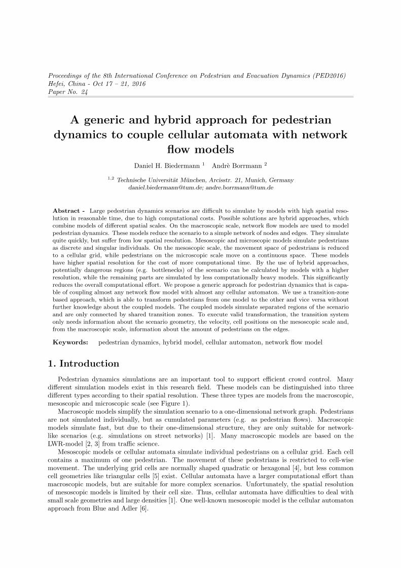
Pedestrian dynamics simulations are an important tool to support efficient crowd control. Manydifferent simulation models exist in this research field. These models can be distinguished into threedifferent types according to their spatial resolution. These three types are models from the macroscopic,mesoscopic and microscopic scale (see Figure 1).

Macroscopic models simplify the simulation scenario to a one-dimensional network graph. Pedestriansare not simulated individually, but as cumulated parameters (e.g. as pedestrian flows). Macroscopicmodels simulate fast, but due to their one-dimensional structure, they are only suitable for network-like scenarios (e.g. simulations on street networks) [1]. Many macroscopic models are based on theLWR-model [2, 3] from traffic science.

Mesoscopic models or cellular automata simulate individual pedestrians on a cellular grid. Each cellcontains a maximum of one pedestrian. The movement of these pedestrians is restricted to cell-wisemovement. The underlying grid cells are normally shaped quadratic or hexagonal [4], but less commoncell geometries like triangular cells [5] exist. Cellular automata have a larger computational effort thanmacroscopic models, but are suitable for more complex scenarios. Unfortunately, the spatial resolutionof mesoscopic models is limited by their cell size. Thus, cellular automata have difficulties to deal withsmall scale geometries and large densities [1]. One well-known mesoscopic model is the cellular automatonapproach from Blue and Adler [6].

Norbert-Schuster-Straße

Schm

iedb

erg

Mühlstraße

Stadtpfarrkirche

Stadttor/Blockhausturm

Albertus-Magnus-Haus

RechtsanwaltHerzog,

Gering undKollegen

Salvatore

Marc

Venezia

Optik Graf

LaufgutEhmann

Merkle

Stadtcafe

2

Macroscopic Scale Mesoscopic Scale Microscopic Scale

Figure 1: From left to right: Simulation scenario on the macroscopic (network flow model), mesoscopic(cellular automaton model) and microscopic scale (continuous model).

Microscopic models provide the highest spatial resolution for the cost of the highest computationaleffort compared to simulation models from other spatial scales. These models simulate individual pedes-trians on a continuous simulation scenario. This means that their spatial resolution is unrestricted. Awell-known example of microscopic models is the social force model developed by Helbing et al. [7].

A simulation of large scenarios with thousands of pedestrians is quite time-consuming for microscopicand mesoscopic pedestrian dynamics models. This aspect gets even more important if we consider pedes-trian dynamic simulators for crowd managers. These users need fast and accurate simulation results toforecast critical situations on the fly. Unfortunately, a high spatial resolution is computationally costlybut necessary to obtain realistic simulation results. Hybrid modeling helps to overcome this issue. Ahybrid approach combines pedestrian dynamics models from different spatial scales. Different regionsof the simulation scenario are calculated by different pedestrian dynamics models. This reduces thecomputational effort, since only regions of special interest are simulated in high spatial resolution. Lessinteresting regions of the scenario are calculated by models with a lower spatial resolution and thereforethey have a lower computational cost. This results in a low overall simulation time, while still providinghigh resolution results for critical regions (e.g. regions with high pedestrian densities or bottlenecks).Different hybrid models exist in the field of pedestrian dynamics [8]. These models are able to combinespecific and predefined models from different scales.

Unfortunately, hybrid models leak a broader and more generic approach. If one of the two combinedmodels is exchanged with a new model, a completely new coupling behavior has to be developed. Thus,the exchange of the coupled mesoscopic or macroscopic model automatically results in the necessity tomake a new coupling procedure. This significantly complicates and decelerates the development of newhybrid models: a generic hybrid approach helps researchers to model new hybrid models in a faster way.Furthermore, already known macroscopic and mesoscopic models can be combined to create new hybridapproaches without much effort. Generic hybrid modeling approaches are currently quite unknown inthe field of pedestrian dynamics [8]. In a first approach, we developed a generic model for the couplingof mesoscopic and microscopic models [9]. But a generic approach for the coupling of mesoscopic andmacroscopic models is still missing. Therefore, we present a generic hybrid model which is able to combinealmost any mesoscopic model with almost any macroscopic pedestrian dynamics model. This is done bya transition system which transforms pedestrians between different scales.

2. Methodology

2.1. Axioms for the transition system

Our generic transition approach is based on a small set of axioms. These axioms are conditionswhich we assume as generally valid for mesoscopic and/or macroscopic simulation models in the fieldof pedestrian dynamics. If the mandatory axioms are valid for a pair of mesoscopic and macroscopicmodels, we can guarantee that our transition system is able to couple these two simulation models intoone hybrid simulation approach. The mandatory and optional axioms are described in Table 1.

Both models, the mesoscopic and the macroscopic one, need to have an upper velocity limit vmax. An

24 - 2

Table 1: Overview of mandatory and optional axioms for the transition system.

Mandatory Conditions Explanation Model

vmax upper boundary for the velocity of pedestrians both∆tmacro ≥ ∆tmeso constant duration of time steps bothNj “source” and “sink” node, connected to the trans-

formation zonemacroscopic

~Nj position of node Nj macroscopicEj bi-directed edge, connected to node Nj macroscopic~eEj unit vector for the direction of edge Ej macroscopicΦEj pedestrian flow on edge Ej macroscopicPi individual and pedestrian mesoscopiccm,n = empty, occupied grid cells which are empty, occupied by obstacles or

by one pedestrianmesoscopic

~cm,n cell center position of cell cm,n mesoscopic~oi current cell position of pedestrian Pi mesoscopic~zi position of the current target of pedestrian Pi mesoscopic

Optional Conditions Explanation Model

vEj local mean velocity of edge Ej macroscopic~vi current velocity of pedestrian Pi mesoscopic~vd,i desired velocity of pedestrian Pi mesoscopic

upper velocity limit means that no pedestrian can have a higher velocity than vmax. This is importantto ensure a limited width of our transformation zone (see Section 2.2). A mesoscopic pedestrian can onlybe transformed if he or she enters this transition zone. The transition zone itself has the geometry ofa circular ring which surrounds the mesoscopic region. This convex shape simplifies the transformationprocedure (see Section 2.4).

Furthermore, both models have to be simulated in constant simulation time steps. These time steps∆tmeso (mesoscopic model) and ∆tmacro (macroscopic model) can be different, but need to have a constantduration. This ensures a smooth connection of simulation models (see Section 2.2). Since a mesoscopicsimulation model has a higher spatial resolution than the macroscopic one, a higher time resolution isnecessary. Therefore, we can assume the relation ∆tmacro ≥ ∆tmeso.

The macroscopic model has to contain a representation of pedestrians, e.g. as a pedestrian flow ΦEj .The pedestrian flow ΦEj is defined as the number of pedestrians n who cross a network edge in a giventime interval. Parameter ρEj describes the density, AEj the area, sEj the length and wEj the width ofedge Ej.

ΦEj (t) =nEj∆t

=ρEj ·AEj

∆t=ρEj · sEj · wEj

∆t(1)

A macroscopic model consists of a network of nodes and edges. It is necessary, that at least one node Nj

of the macroscopic network is located inside of the transition zone. Its position ~Nj , which is part of themacroscopic network, has to be known by the transition system. Otherwise, no connection exists betweenthe macroscopic model and the transition system. The macroscopic network flow model has to handlethis node Nj as a “source” and as a “sink” for its pedestrian flows. In this context, “sink” means that themacroscopic model has to remove all pedestrian flows which reach this node Nj. “Source” means that themacroscopic model can generate new pedestrians in this node Nj based on the information given by thetransition system. If no “sink” or “source” would exist in node Nj, no macroscopic pedestrian flow couldenter or leave the transition zone. It is necessary, that the unit vector (|~eEj | = 1) of the direction ~eEj ofedge Ej is known by the transition system. This edge Ej has to be connected to node Nj. An importantbut not necessary parameter is the local mean velocity vEj on the edges connected to the transition zone.If this parameter does not exist, the standard velocity distribution [10] is used to calculate this value (seeSection 2.3).

The mesoscopic model is a cellular automaton. Thus, the mesoscopic simulation model has to containindividual pedestrian agents Pi and grid cells cm,n. A grid cell cm,n is either empty or occupied. Onegrid cell is occupied by obstacles or by exactly one pedestrian Pi. Each existing pedestrian Pi in themesoscopic model has to be assigned to a grid cell cm,n with its cell center at ~cm,n. The assigned cell

24 - 3

Obstacle

Transition Zone

MacroscopicEdge Ej

MacroscopicNode Nj

Pedestrian Pi

Mesoscopic Region

Figure 2: Transition Zone (green region) as a point of connection between mesoscopic (light red region)and macroscopic (blue network) models

gives the pedestrian’s current cell position ~oi. Additionally, each pedestrian Pi needs a target ~zi he orshe is currently heading to. Optional parameters are the current velocity ~vi and desired velocity ~vd,iof a mesoscopic pedestrian Pi. If these parameters are not available in the mesoscopic model, they canbe estimated by the pedestrians’ position of the last time step or by the standard velocity distribution[10]. Mostly all mesoscopic and macroscopic simulation models meet the axioms described in this section.Therefore, we propose that our transition system is able to combine the largest amount of mesoscopicand macroscopic models currently available in literature.

2.2. Structure of the transition system

Our generic hybrid scenario contains three different region types: the macroscopic network region,the region of the mesoscopic cellular automaton and a transition zone which connects these regions (seeFigure 2). The transition zone ensures that macroscopic pedestrian flows ΦEj can be transformed intomesoscopic pedestrians Pi and vice versa. Sections 2.3 and 2.4 describe this transformation behavior indetail.

According to our axioms, macroscopic and mesoscopic models are simulated in discrete simulation timesteps. Our transition system checks after each macroscopic time step if a transformation of macroscopicpedestrian flows ΦEj or mesoscopic pedestrians Pi is necessary. Only macroscopic pedestrian flows onedge Ej and mesoscopic singular pedestrians, which are part of the transition zone, can be transformed.Thus, our transition zone has to be wide enough that no pedestrian can leave the region of his or hercurrent simulation model without entering the transition zone. Since the transformations take place aftereach macroscopic simulation time step ∆tmacro, the minimum necessary width dtrans of the transitionzone is described by

dtrans ≥ ∆tmacro · vmax (2)

The minimal width dtrans for the transition zone ensures that all pedestrians are forced to enter the tran-sition zone, if they leave the region of their current simulation model. This ensure that these pedestrianscan be transformed into the macroscopic scale.

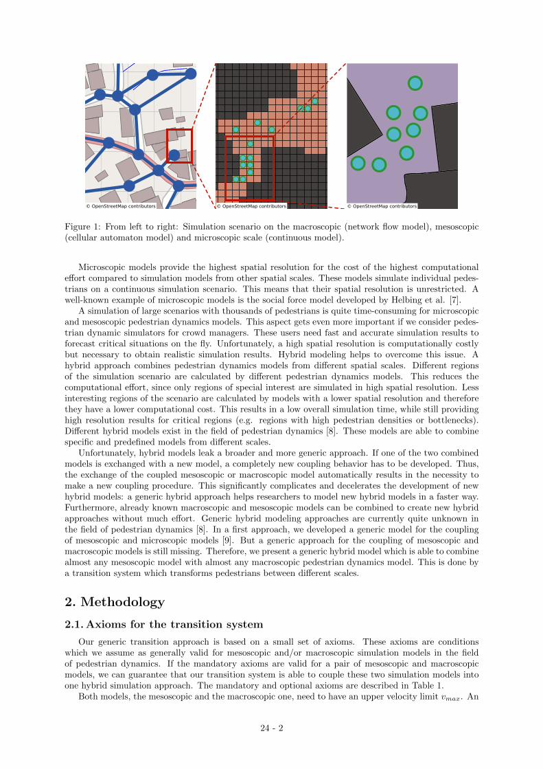
The macroscopic and the mesoscopic simulation models can have different long time step durations.Since the transformation procedure is executed after each macroscopic time step ∆tmacro, the positionsof mesoscopic pedestrians Pi in the transition zone have to be synchronized (see Figure 3). If we haveexecuted k macroscopic time steps ∆tmacro and l mesoscopic time steps ∆tmeso, we can determine theasynchronous time gap ∆asynch for the mesoscopic pedestrians as:

∆asynch = k ·∆tmacro − l ·∆tmeso (3)

The transformation of pedestrians is executed after each macroscopic time step. This means the timeduration between two transformation processes equals ∆tmacro. Thus, we need to predict the positionsof mesoscopic pedestrians Pi at this transformation time Tk = k ·∆tmacro based on their positions at the

24 - 4

∆tmeso

∆tmacroSimulated Time t ∆asynch

k + 2k + 1kk, l = 0

l − 1l − 2 l + 2l + 1l

k − 1

Figure 3: Asynchronous time line for macroscopic (blue bar) and mesoscopic (light red bar) time steps.The transformation (green bar) is executed after each macroscopic time step.

Obstacle

Transition Zone

Mesoscopic Region

Pedestrian Pi

vmax ·∆tmacro

eEj

Nj

ΦEj P i

Φ→Ej(t)

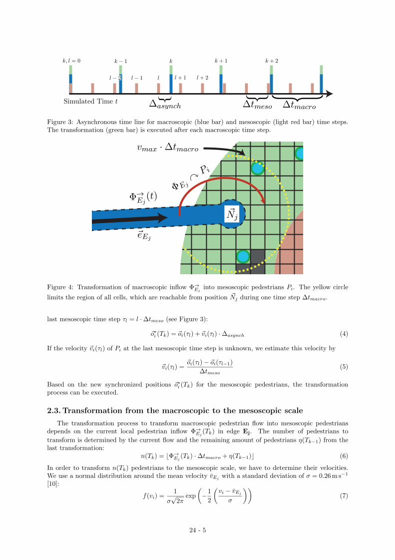
Figure 4: Transformation of macroscopic inflow Φ→Ej into mesoscopic pedestrians Pi. The yellow circle

limits the region of all cells, which are reachable from position ~Nj during one time step ∆tmacro.

last mesoscopic time step τl = l ·∆tmeso (see Figure 3):

~o∗i (Tk) = ~oi(τl) + ~vi(τl) ·∆asynch (4)

If the velocity ~vi(τl) of Pi at the last mesoscopic time step is unknown, we estimate this velocity by

~vi(τl) =~oi(τl)− ~oi(τl−1)

∆tmeso(5)

Based on the new synchronized positions ~o∗i (Tk) for the mesoscopic pedestrians, the transformationprocess can be executed.

2.3. Transformation from the macroscopic to the mesoscopic scale

The transformation process to transform macroscopic pedestrian flow into mesoscopic pedestriansdepends on the current local pedestrian inflow Φ→Ej (Tk) in edge Ej. The number of pedestrians to

transform is determined by the current flow and the remaining amount of pedestrians η(Tk−1) from thelast transformation:

n(Tk) = bΦ→Ej (Tk) ·∆tmacro + η(Tk−1)c (6)

In order to transform n(Tk) pedestrians to the mesoscopic scale, we have to determine their velocities.We use a normal distribution around the mean velocity vEj with a standard deviation of σ = 0.26 m s−1

[10]:

f(vi) =1

σ√

2πexp

(−1

2

(vi − vEj

σ

))(7)

24 - 5

This calculation is repeated, if the calculated velocity vi for a mesoscopic pedestrian Pi exceeds vmax. Ifthe mean velocity vEj is unavailable, the normal mean velocity v = 1.34 m s−1 is used instead [10]. The

optimal position ~Oi to put the pedestrian into the mesoscopic scale is based on the pedestrian’s velocityvi, the direction ~eEj of edge Ej and the position ~Nj of node Nj. We calculate the position a pedestrianhas most likely reached during the last macroscopic time step by:

~Oi(Tk) = ~Nj + vi · ~eEj ·∆tmacro (8)

If the mesoscopic cell at this position is free, the pedestrian Pi is generated at this cell. Otherwise,we rate all cells reachable by this pedestrian due to their suitability. Reachable cells are all free cellscm,n inside the transition zone with | ~Nj − ~cm,n ≤ vmax · ∆tmacro|. We rate these cells according to

their similarity to the ideal cell position ~Oi(Tk) and choose the cell cm,n with the lowest rating value

R = | ~Oi(Tk) − ~cm,n|. If no free cell is reachable, the pedestrian remains macroscopic. Afterwards, thedescribed calculation is executed for remaining pedestrian until this process repeats for all pedestriansn(Tk). After this procedure, we have transformed nmeso(Tk) ≤ n(Tk) pedestrians to the mesoscopic scale.The amount of pedestrians remaining macroscopic in edge Ej is calculated by:

η(Tk) = ΦEj (Tk) ·∆tmacro + η(Tk−1)− nmeso(Tk) (9)

We are able to transform macroscopic pedestrian flows ΦEj into discrete mesoscopic pedestrians Pi.The transformation is executed undisturbed under normal circumstances. Normal circumstances mean,taht the number of pedestrians in the transition zone is not too high. Unfortunately, if the pedestriandensity increases, crowd congestions can arise either for the macroscopic or the mesoscopic scale. A crowdcongestion for a macroscopic edge Ej occurs, if not all pedestrians of the inflow Φ→Ej (Tk) can be placed

on free and reachable cells (see Figure 4). In the case of such crowd congestions, the further inflow isstopped for the next macroscopic time step. During the next transformation, the transition system triesto place the remaining pedestrians into the mesoscopic scale according to the procedure described in thissection.

2.4. Transformation from the mesoscopic to the macroscopic scale

For the transformation of mesoscopic pedestrians Pi into a macroscopic network, we have to determinewhich pedestrians inside the transition zone are heading towards the region of the macroscopic scale. Wecalculate the projected position ~o+i (Tk+1) the pedestrian Pi would reach, if he or she walks with maximalvelocity into his or her current direction:

~o+i (Tk+1) = ~o∗i (Tk) +~vi(τl)

|~vi(τl)|· vmax ·∆tmacro (10)

If the projected position ~o+i (Tk+1) of pedestrian Pi is located in the macroscopic scale, a transformationof this pedestrian is necessary. Otherwise, the convex shape of the transition zone guarantees thatpedestrians, who keep their walking direction, will not leave the mesoscopic region during the nextmacroscopic time step. This approach has one limitation: if pedestrians change their current walking

direction~vi(τl)|~vi(τl)|

during the next macroscopic time step ∆tmacro, it is possible that they would leave the

mesoscopic region without being transformed to the macroscopic region. Thus, we have to include thepossibility of direction change in our approach. Pedestrians do not change their direction suddenly butchange it slightly, stride by stride. For a direction change, the average change of angle per stride equalsωs = ±12.3 [11]. The human stride length varies between 0.5 m for low velocities and 2.2 m for highvelocities [10]. According to [10, 12], the relationship between velocity vi and stride length ds is describedby:

ds(vi) = 0.234 m + 0.302 m · vi (11)

The maximal possible change of angle ±Ω depends on the maximal number of strides a pedestrian cantake during the next macroscopic time step:

±Ω = ±∆tmacro · vids(vi)

· |ωs| (12)

Naturally, the maximal change of angle is limited by ±Ωmax = ±π. This maximal angle means that

24 - 6

Obstacle

Transition ZonePedestrian Pi

eEj

Nj

Φ←Ej(t)

P1

P2

Walking Direction

Pedestrian Pi

Pedestrian PiPedestrian Pi

+Ω

+Ω

−Ω

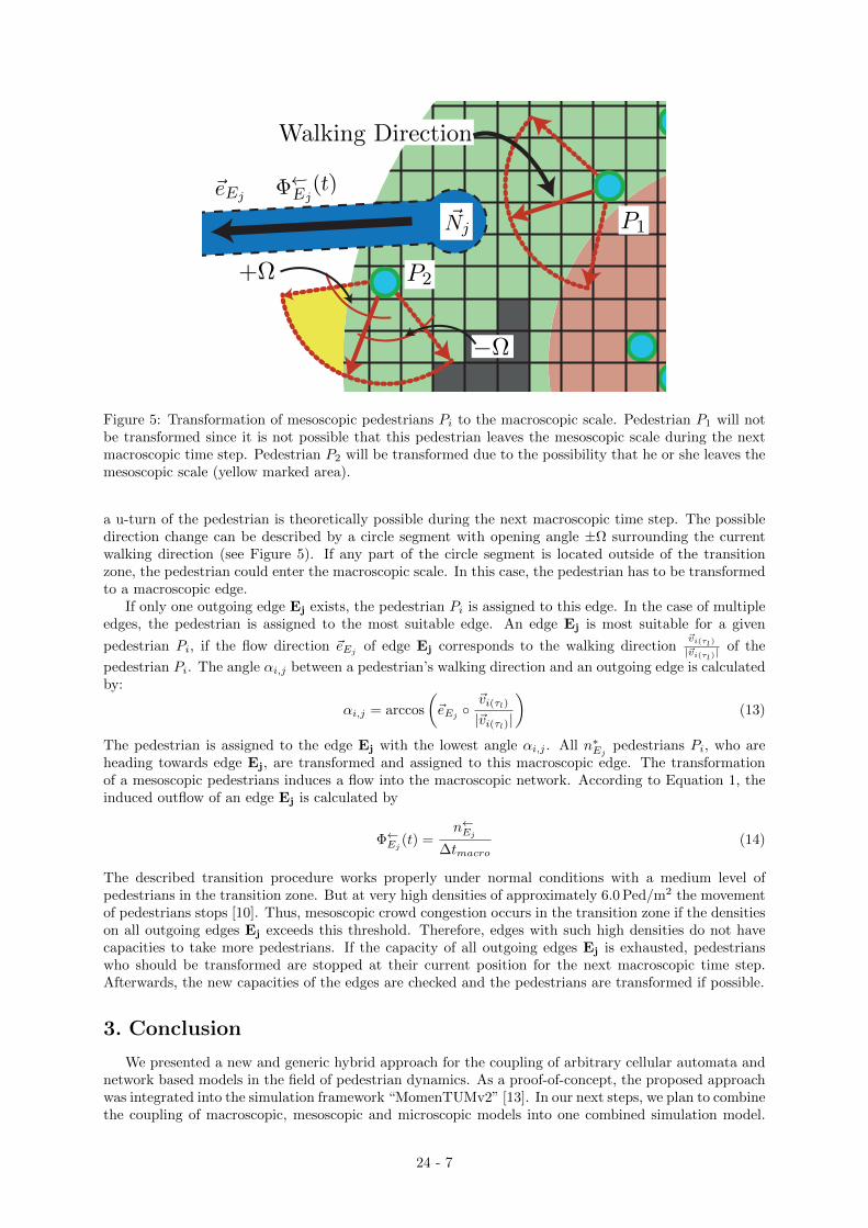
Figure 5: Transformation of mesoscopic pedestrians Pi to the macroscopic scale. Pedestrian P1 will notbe transformed since it is not possible that this pedestrian leaves the mesoscopic scale during the nextmacroscopic time step. Pedestrian P2 will be transformed due to the possibility that he or she leaves themesoscopic scale (yellow marked area).

a u-turn of the pedestrian is theoretically possible during the next macroscopic time step. The possibledirection change can be described by a circle segment with opening angle ±Ω surrounding the currentwalking direction (see Figure 5). If any part of the circle segment is located outside of the transitionzone, the pedestrian could enter the macroscopic scale. In this case, the pedestrian has to be transformedto a macroscopic edge.

If only one outgoing edge Ej exists, the pedestrian Pi is assigned to this edge. In the case of multipleedges, the pedestrian is assigned to the most suitable edge. An edge Ej is most suitable for a given

pedestrian Pi, if the flow direction ~eEj of edge Ej corresponds to the walking direction~vi(τl)|~vi(τl)|

of the

pedestrian Pi. The angle αi,j between a pedestrian’s walking direction and an outgoing edge is calculatedby:

αi,j = arccos

(~eEj

~vi(τl)

|~vi(τl)|

)(13)

The pedestrian is assigned to the edge Ej with the lowest angle αi,j . All n∗Ej pedestrians Pi, who areheading towards edge Ej, are transformed and assigned to this macroscopic edge. The transformationof a mesoscopic pedestrians induces a flow into the macroscopic network. According to Equation 1, theinduced outflow of an edge Ej is calculated by

Φ←Ej (t) =n←Ej

∆tmacro(14)

The described transition procedure works properly under normal conditions with a medium level ofpedestrians in the transition zone. But at very high densities of approximately 6.0 Ped/m2 the movementof pedestrians stops [10]. Thus, mesoscopic crowd congestion occurs in the transition zone if the densitieson all outgoing edges Ej exceeds this threshold. Therefore, edges with such high densities do not havecapacities to take more pedestrians. If the capacity of all outgoing edges Ej is exhausted, pedestrianswho should be transformed are stopped at their current position for the next macroscopic time step.Afterwards, the new capacities of the edges are checked and the pedestrians are transformed if possible.

3. Conclusion

We presented a new and generic hybrid approach for the coupling of arbitrary cellular automata andnetwork based models in the field of pedestrian dynamics. As a proof-of-concept, the proposed approachwas integrated into the simulation framework “MomenTUMv2” [13]. In our next steps, we plan to combinethe coupling of macroscopic, mesoscopic and microscopic models into one combined simulation model.

24 - 7

Doing so, we obtain a holistic and generic simulation framework to simulate large and complex scenariosin a fast and accurate way. However, some limitations exist for our generic approach. It is essentialthat all mandatory conditions given in Table 1 are valid for the macroscopic and mesoscopic model.Otherwise, a coupling of these two models is not possible with our approach. However, according toour literature research, most macroscopic and mesoscopic models fulfill these conditions. The introducedgeneric transformation comes at the cost of losing model specific attributes. Some specific attributes ofpedestrian dynamics models are difficult or even impossible to transform between different scales. Forexample, the social aspect of group behavior (e.g. [14]) depends on individual agents. Since macroscopicmodels consider cumulated parameters instead of individual pedestrian agents, they are not able tomodel such behavior. Therefore, such specific attributes get lost if pedestrians are transformed to themacroscopic scale.

Acknowledgments

We would like to thank all members of the MultikOSi project, especially our colleague Peter M. Kielar,for their helpful discussions according to this topic. This work is supported by the Federal Ministry forEducation and Research (Bundesministerium fur Bildung und Forschung, BMBF), project MultikOSi,under grant FKZ 13N12823.

References

[1] D. H. Biedermann et al., “A hybrid and multiscale approach to model and simulate mobility in thecontext of public event,” in Transportation Research Procedia, 2016.

[2] M. J. Lighthill and G. B. Whitham, “On kinematic waves. II. A theory of traffic flow on long crowdedroads,” in Proceedings of the Royal Society of London A: Mathematical, Physical and EngineeringSciences, vol. 229, no. 1178, pp. 317-345, 1955.

[3] P. I. Richards, “Shock waves on the highway,” in Operations research, vol. 4, no. 1, pp. 42-51, 1956.

[4] C. P. D. Birch et al., “Rectangular and hexagonal grids used for observation, experiment and simu-lation in ecology,” in Ecological Modelling, vol. 206, no. 3, pp. 293-32, 2007.

[5] M. Chen et al., “Modeling Pedestrian Dynamics on Triangular Grids,” in Transportation ResearchProcedia, vol. 2, pp. 327-335, 2014.

[6] V. J. Blue and J. L. Adler, “Cellular automata microsimulation for modeling bi-directional pedestrianwalkways,” in Transportation Research Part B: Methodological, vol. 35, no. 3, pp. 293-312, 2001.

[7] D. Helbing et al., “Simulation of pedestrian crowds in normal and evacuation situations,” in Pedes-trian and Evacuation Dynamics, pp 21-58, 2002.

[8] K. Ijaz et al., “A Survey of Latest Approaches for Crowd Simulation and Modeling using HybridTechniques,” in 17th UKSIMAMSS International Conference on Modelling and Simulation, pp. 111-116, 2015.

[9] D. H. Biedermann et al., “Towards TransiTUM: A Generic Framework for Multiscale Coupling ofPedestrian Simulation Models based on Transition Zones,” in Transportation Research Procedia, vol.2, pp. 495-500, 2014.

[10] U. Weidmann, Transporttechnik der Fussgnger: Transporttechnische Eigenschaften desFussgangerverkehrs (Literaturauswertung). Zurich, Schriftenreihe des IVT, 1992.

[11] G. Antonini et al., “Discrete choice models of pedestrian walking behavior,” in Transportation Re-search Part B, vol. 40, pp. 667-687, 2006.

[12] R. Magaria, Biomechanics and energetics of muscular exercise. Oxford, Clarendon Press, 1976.

[13] Kielar et al., “MomenTUMv2: a modular, extensible, and generic agent-based pedestrian behaviorsimulation framework,” Technical Report, 2016.

[14] M. Moussaid et al., “The Walking Behaviour of Pedestrian Social Groups and Its Impact on CrowdDynamics,” in Plos One, vol. 5, no. 4, 2010.

24 - 8