a framework for construction of and computations on four...
TRANSCRIPT

Page 1
A Framework for construction of and computations
on Four-Dimensional Aircraft Trajectories
CMSC 663-664
2016-2017
Author:
Jon Dehn
Advisor:
Dr. Sergio Torres
Fellow, Leidos Corporation
Final Report – May 12, 2017

Page 2
Abstract
Air traffic control systems perform many functions in order to safely and efficiently move air
traffic through the national and international airspace. A key component of these systems is an
accurate prediction of where the individual flights will be over time. This project builds a
framework to both do that prediction and use the prediction to examine various air traffic
control algorithms for both accuracy and efficiency. This framework is designed for reuse, such
that future research into ATC algorithms can be conducted with simple extensions to the
system.

Page 3
Table of Contents 1 Introduction .......................................................................................................................................... 6
2 Project Goal ........................................................................................................................................... 6
3 Approach ............................................................................................................................................... 7
4 Scientific Computing Algorithms ........................................................................................................... 8
4.1 Background Concepts ................................................................................................................... 8
4.1.1 Coordinate system ................................................................................................................ 8
4.1.2 Speed Definitions .................................................................................................................. 8
4.2 Trajectory Generation ................................................................................................................... 9
4.2.1 Trajectory Generation Basics – latitude and longitude dimension ....................................... 9
4.2.2 Trajectory generation basics – altitude and time ............................................................... 10
4.2.3 Rate of Climb/Descent ........................................................................................................ 11
4.2.4 Trajectory Generation Inputs .............................................................................................. 14
4.2.5 Trajectory Generation Details ............................................................................................. 15
4.3 Use of Weather Forecast Models ............................................................................................... 16
4.4 Wind Optimal Trajectories .......................................................................................................... 17
4.4.1 Version 1 ............................................................................................................................. 18
4.4.2 Version 2 ............................................................................................................................. 20
4.5 Parallelizing Conflict Detection ................................................................................................... 21
4.5.1 Time Filter ........................................................................................................................... 23
4.5.2 Horizontal Filter .................................................................................................................. 24
4.5.3 Parallelization Strategies ..................................................................................................... 27
5 Implementation .................................................................................................................................. 31
6 Validation Methods ............................................................................................................................. 31
7 Test Problems for Verification ............................................................................................................ 33
7.1 Use of Weather Forecast Models ............................................................................................... 33
7.2 Wind Optimal Trajectories .......................................................................................................... 33
7.3 Parallelizing Conflict Detection ................................................................................................... 33
8 Results ................................................................................................................................................. 34
8.1 Use of Weather Forecasts ........................................................................................................... 34
8.1.1 Quality of Forecast .............................................................................................................. 34
8.1.2 Impact on Flight Time ......................................................................................................... 35
8.2 Wind Optimal Trajectories .......................................................................................................... 37

Page 4
8.3 Parallel Processing ...................................................................................................................... 37
9 Conclusion ........................................................................................................................................... 40
Appendix A. Timeline ............................................................................................................................... 40
Appendix B. Milestones ........................................................................................................................... 40
Appendix C. Deliverables ......................................................................................................................... 41
Appendix D. Bibliography ........................................................................................................................ 41
Appendix E. List of Abbreviations ........................................................................................................... 41

Page 5
List of Figures Figure 1 Framework Design .......................................................................................................................... 7
Figure 2 Horizontal path for sample flight .................................................................................................. 10
Figure 3 Vertical profile of sample flight ..................................................................................................... 11
Figure 4 Lambert vs. Spherical grids ........................................................................................................... 15
Figure 5 Flights Paths for the Use of Forecasted Weather analysis............................................................ 17
Figure 6 Wind Optimal Trajectories, Version 1 ........................................................................................... 19
Figure 7 Wind Optimal Trajectories, Version 2 ........................................................................................... 21
Figure 8 Conflict Detection Time Filter ....................................................................................................... 23
Figure 9 Conflict Detection Altitude Filter .................................................................................................. 23
Figure 10 Conflict Detection Horizontal Filter - part 1 ................................................................................ 24
Figure 11 Conflict Detection Horizontal Filter - part 2 ................................................................................ 25
Figure 12 Conflict Detection Horizontal Filter - part 3 ................................................................................ 25
Figure 13 Conflict Detection Horizontal Filter - part 4 ................................................................................ 26
Figure 14 Conflict Detection Horizontal Filter - part 5 ................................................................................ 26
Figure 15 Conflict Detection Horizontal Filter - part 6 ................................................................................ 27
Figure 16 NVIDIA CPU/GPU Architecture.................................................................................................... 28
Figure 17 Memory moves for strategy 2 .................................................................................................... 29
Figure 18 Memory moves for strategy 3 .................................................................................................... 30
Figure 19 Trajectory Generation Comparison ............................................................................................ 32
Figure 20 Effect of Wind on Trajectories .................................................................................................... 33
Figure 21 Test flights used for Conflict Detection ....................................................................................... 34
Figure 22 Accuracy of Forecasted Wind Speed........................................................................................... 35
Figure 23 Distribution of flight time differences with forecasted weather ................................................ 36
Figure 24 Summary of Flight Time Errors ................................................................................................... 37

Page 6
1 Introduction Global Air Traffic Control (ATC) is distributed among multiple Flight Information Regions (FIRs). Each
country is responsible for safely and efficiently handling traffic in their FIRs. Most countries have 1 FIR;
due to the volume of air traffic and the complexity of its airspace, the US has 20.
At the core of the FIR’s processing is building an estimate of each aircraft’s trajectory (a four dimensional
description of the flight path, with dimensions of latitude, longitude, altitude and time).
Once these trajectories are constructed, they are used for various purposes, such as conflict detection
(which predicts whether two aircraft will be too close to each other, or if a single aircraft will fly into
restricted airspace), workload planning for the human controllers separating air traffic, airport arrival
and departure planning, etc.
This project examines different aspects of generating and using these trajectories, including
performance aspects of using the trajectories in various applications.
2 Project Goal The project has built a modular system where:
1. Different trajectory generation algorithms can be tested
2. Algorithms using those trajectories can be tested for performance and accuracy. The specific
algorithms selected have relevance to the state of the practice today.
This framework can be used to explore new concepts for air traffic management.
A secondary goal is that the project’s author becomes familiar with techniques of parallelizing
computing algorithms, and becomes more proficient in the use of the Python programming language.
Page 7
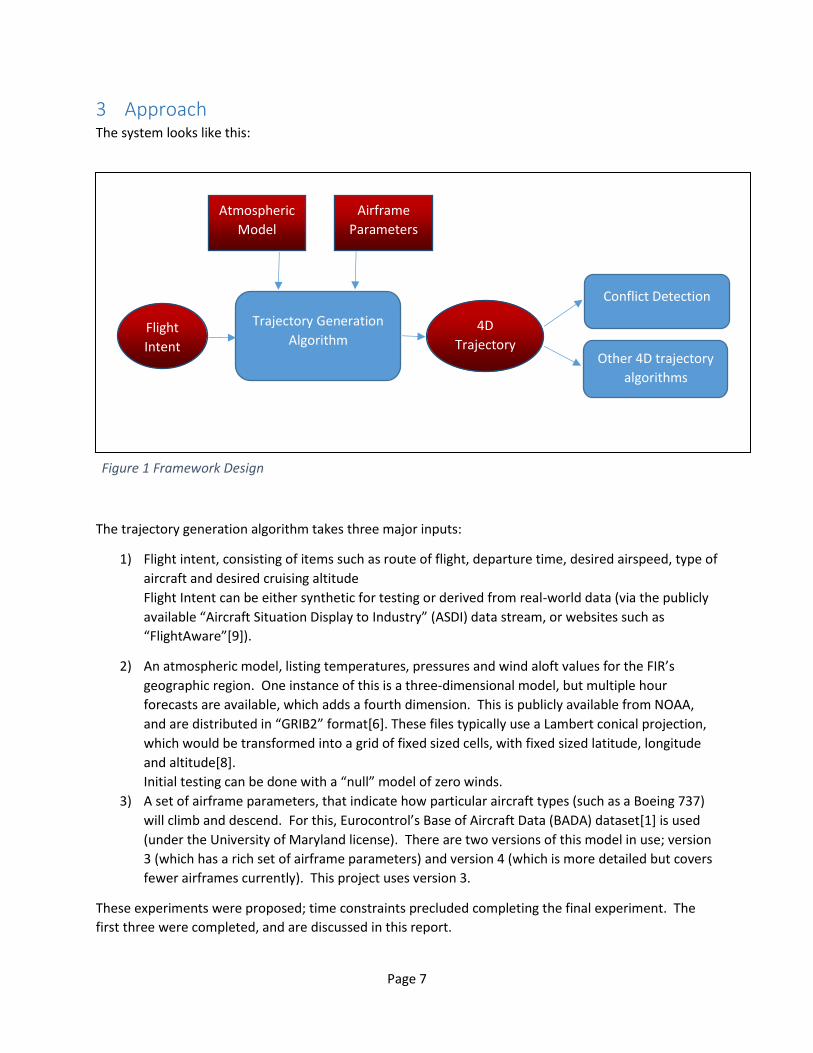
3 Approach The system looks like this:
The trajectory generation algorithm takes three major inputs:
1) Flight intent, consisting of items such as route of flight, departure time, desired airspeed, type of
aircraft and desired cruising altitude
Flight Intent can be either synthetic for testing or derived from real-world data (via the publicly
available “Aircraft Situation Display to Industry” (ASDI) data stream, or websites such as
“FlightAware”[9]).
2) An atmospheric model, listing temperatures, pressures and wind aloft values for the FIR’s
geographic region. One instance of this is a three-dimensional model, but multiple hour
forecasts are available, which adds a fourth dimension. This is publicly available from NOAA,
and are distributed in “GRIB2” format[6]. These files typically use a Lambert conical projection,
which would be transformed into a grid of fixed sized cells, with fixed sized latitude, longitude
and altitude[8].
Initial testing can be done with a “null” model of zero winds.
3) A set of airframe parameters, that indicate how particular aircraft types (such as a Boeing 737)
will climb and descend. For this, Eurocontrol’s Base of Aircraft Data (BADA) dataset[1] is used
(under the University of Maryland license). There are two versions of this model in use; version
3 (which has a rich set of airframe parameters) and version 4 (which is more detailed but covers
fewer airframes currently). This project uses version 3.
These experiments were proposed; time constraints precluded completing the final experiment. The
first three were completed, and are discussed in this report.
Atmospheric
Model
Airframe
Parameters
Trajectory Generation
Algorithm Flight
Intent
4D
Trajectory
Conflict Detection
Other 4D trajectory
algorithms
Figure 1 Framework Design

Page 8
1) The current US system uses current-hour weather model for all computations, even though a
flight can last several hours. Implement a version that uses future weather forecasts and
compare changes in long-duration trajectories
2) Find an optimal wind-aided trajectory. This will find an “optimal” trajectory between two points
given non-zero wind patterns. Initially, “optimal” will be define as the trajectory that uses the
least fuel; other more complex definitions could be supplied.
3) Parallelize conflict detection algorithms, measure complexity of implementation vs. speed
tradeoffs for different parallel techniques
4) Look at the increased accuracy of BADA version 3 vs. version 4 for identical aircraft types,
balanced against the increase in complexity and computational load
The algorithms for each experiment are described in the next section.
4 Scientific Computing Algorithms The principal algorithm that is implemented is the generation of the 4D trajectory; this requires the
solution of the ordinary differential equation to describe the climb and descent segments of the
trajectory. Some basic concepts are discussed first.
4.1 Background Concepts
4.1.1 Coordinate system Points on the earth’s surface are transformed to a Cartesian coordinate (x,y,z) on a unit sphere (radius =
1.0). Given the radius of the earth, distances on the surface of the unit sphere are converted to nautical
miles (NMI), for things like speed calculations (Knots). Other calculations such as intersection of great
circle arcs are simplified when the unit sphere is used.
Since we are concerned with a particular geographic area, an approximation of the earth’s radius for
that area would be used in practice (perhaps slightly different for each FIR). For this project, the mean
radius of the earth will be used.
All external latitude/longitudes are supplied in WGS 84 coordinates[2], which assumes the earth is an
ellipsoid with specific major and minor axes (same as is used by the GPS). Translation to the unit sphere
is straight forward, and supplied as routines in many programming languages.
Note that the Cartesian coordinate (x/y/z) is for the surface of the earth. Altitude above the surface is
separately specified (and forms one dimension of each trajectory point). This simplifies the ODE to be
solved, since it depends on altitude, not distance from the earth’s center.
4.1.2 Speed Definitions The algorithms use several different “speed” values, as described below.
True Airspeed (TAS) – speed of the aircraft relative to the surrounding air mass (which may be moving
with respect to the earth’s surface)

Page 9
Ground speed – speed of the aircraft over the surface of the earth; this is the true airspeed adjusted by
the winds moving the air mass. If wind speed and TAS are given as vectors, VGS = VTAS + VWIND.
Calibrated airspeed (CAS) – airspeed as known to the aircraft’s instrumentation; this is based on a
“calibration” that takes into account any known bias in the instruments. For a constant CAS, TAS will
vary depending on altitude
Mach – speed of sound; important here because aircraft plan to hold CAS and Mach constant; there is a
crossover altitude at above which planning is done based on Mach speed, CAS and Mach will be equal at
that altitude.
4.2 Trajectory Generation
4.2.1 Trajectory Generation Basics – latitude and longitude dimension As noted above, the trajectory generator takes flight intent as an input. This is supplied by the airline or
pilot, and consists of:
• The path (over the surface of the earth) to be followed
• The desired cruise altitude
• The desired cruise speed (true airspeed or Mach; in practice only military flights specify this in
Mach)
• The type of airplane (e.g. Boeing 737)
• Departure time
As an example, consider Southwest flight 3156 from Baltimore (airport code BWI) to Orlando (MCO):
• altitude 40,000 feet
• speed 452 knots
• Boeing 737-300
• Depart at 10:35 am
The creation of the actual path from departure airport to destination airport is beyond the scope of this
project; we start with the expanded set of points as an input. This input defines a path on the earth’s
surface, which starts at the departure airport, ends at the destination airport, and has intermediate
waypoints. The waypoints are connected by great circle arcs. In order to more accurately follow the
path of the flight, turn waypoints can be replaced with a number of smaller segments that more closely
approximate the turn to be taken. Whether this is done depends on the accuracy needed for other
work. Figure 2 shows an example path from Baltimore to Orlando.

Page 10
Figure 2 Horizontal path for sample flight
4.2.2 Trajectory generation basics – altitude and time In order to turn the two-dimensional waypoints into points on a four-dimensional trajectory, altitude
and time are calculated for each point. This results in a vertical profile that looks something like Figure
3.

Page 11
Figure 3 Vertical profile of sample flight
Each trajectory point is called a cusp, and the segments that connect cusps have a constant rate of
vertical velocity (climb or descent) and a constant rate of acceleration over the segment. This, along
with the starting ground speed for each segment, allows us to predict where a flight will be at any point
in time.
This final representation of the trajectory has additional points added between the waypoints supplied
as inputs, in order to assure that the above definition of constant acceleration/vertical velocity holds.
For example, it is necessary to accelerate to the desired climb speed; when that acceleration is complete
a cusp is added to the trajectory.
4.2.3 Rate of Climb/Descent Calculation of the rate of climb (or descent) is described in detail in [1], and is summarized here.
The basis of this rate is this conservation of energy equation:
(Thr − D) ∗ VTAS = mg0
dh
dt+ mVTAS
dVTAS
dt(4.2.3 − 1)
Where
0
5000
10000
15000
20000
25000
30000
35000
40000
0 50 100 150 200 250 300 350
Alt
itu
de
(Fe
et)
Along Route Distance (NMI)
Python Generated TrajectoryBoeing 735 - Cruise Alt 35,000

Page 12
Thr Thrust supplied by the aircraft engines
m (mass) Mass of the aircraft, including fuel, passangers and baggage. This will decrease over the life of the flight
D (Drag) Drag from movement through the atmosphere
g0 Gravitational acceleration
VTAS Velocity in true airspeed h Geodetic altitude
Combine this equation with the assumption that, during climbs and descents, pilots hold speed (CAS or
Mach) and throttle position constant, the above can be re-written as
dh
dt=
(Thr − D) ∗ VTAS
mg0[1 + (
VTAS
g0) (
dVTAS
𝑑ℎ)]
−1
(4.2.3 − 2)
The last term can be replaced by an “energy share factor” [3]; the ratio of energy allocated to climb vs.
acceleration for a constant velocity; a function of Mach:
𝑓{𝑀} = [1 + (VTAS
g0) (
dVTAS
𝑑ℎ)]
−1
(4.2.3 − 3)
Hence, the rate of climb or descent (which is typically expressed in pressure altitude Hp, rather than
geodetic altitude h), is
𝑅𝑂𝐶𝐷 = 𝑑𝐻𝑝
𝑑𝑡=
𝑇 − ∆𝑇
𝑇[(Thr − D) ∗ VTAS
mg0] 𝑓{𝑀} (4.2.3 − 4)
Where T is temperature at altitude, and ∆𝑇 is the temperature differential at that altitude from the
International Standard Atmosphere (this is given by the atmospheric model).
4.2.3.1 Energy Share Factor
The energy share factor 𝑓{𝑀} is a function of Mach (M) and varies with altitude, and whether we are
accelerating or decelerating in climb or descent. As an example (to convey the complexity of the
equation), below the crossover altitude when not accelerating, it is defined as:
𝑓{𝑀} = {1 +𝜅𝑅𝛽𝑇,<
2𝑔0𝑀2
𝑇 − ∆𝑇
𝑇+ (1 +
𝜅 − 1
2𝑀2)
−1𝜅−1
{(1 +𝜅 − 1
2𝑀2)
𝜅𝜅−1
} − 1}
−1
(4.2.3 − 5)
Where
𝜿 Adiabatic index of air = 1.4 R Real gas constant for air =287.05287

Page 13
𝜷𝑻,< ISA temperature gradient below the tropopause - -0.0065
The Mach number is based on the current speed at the current altitude, which may be a true airspeed.
If so, that TAS is converted to a Mach value by dividing the VTAS by the speed of sound at the given
altitude (the value for T is obtained from the weather model at the current altitude):
𝑀 =𝑉𝑇𝐴𝑆
√𝜅𝑅𝑇(4.2.3 − 6)
The full definition of the energy share factor can be found in [1].
4.2.3.2 Thrust
Thrust depends on the engine type (Jet, Turboprop or Propeller), pressure altitude, airspeed (in some
cases) and temperature differential.
For example, for a jet engine, the maximum climb thrust would be:
(𝑇ℎ𝑟max 𝑐𝑙𝑖𝑚𝑏)𝐼𝑆𝐴 = 𝐶𝑇𝐶,1 ∗ (1 − 𝐻𝑝
𝐶𝑇𝐶,2+ 𝐶𝑇𝐶,3 ∗ 𝐻𝑝
2) (4.2.3 − 7)
Where the coefficients Cx are given for the airframe type in the BADA dataset. Note that in this case (of
a jet engine) there is no term for airspeed.
4.2.3.3 Drag
Drag depends on the Drag Coefficient, which in turn depends on the lift coefficient.
Lift coefficient:
𝐶𝐿 = 2 ∗ 𝑚 ∗ 𝑔0
𝜌 ∗ 𝑉𝑇𝐴𝑆2 ∗ 𝑆 ∗ 𝑐𝑜𝑠∅
(4.2.3 − 8)
Drag Coefficient:
𝐶𝐷 = 𝐶𝐷0,𝐶𝑅 + 𝐶𝐷2,𝐶𝑅 ∗ (𝐶𝐿)2 (4.2.3 − 9)
And finally drag force:
𝐷 = 𝐶𝐷 ∗ 𝜌 ∗ 𝑉𝑇𝐴𝑆
2 ∗ 𝑆
2(4.2.3 − 10)
S Wing surface area ρ Air density ∅ Bank angle (zero, unless in a turn)

Page 14
4.2.3.4 Weather Model
The weather model supplies some key data for the above equations. Specifically, the following
information is used from the NOAA-supplied data:
1) North wind component
2) East wind component
3) Temperature (from which the ∆𝑇 can be calculated)
4) Pressure
4.2.4 Trajectory Generation Inputs
4.2.4.1 Flight Intent Source
The FlightAware web site (www.flightaware.com) provides intent (airspeed, cruise altitude, route of
flight, departure time) for all commercial flights in the US. Once a pair of endpoint airports is selected,
that site provides the fixes in the route for a variety of flights between those cities. This data is screen-
scraped (using a developed Python program) to produce an intent file that can be used in various
experiments.
Flights of various durations and directions can therefore be added to the inventory of test data.
4.2.4.2 Airframe Parameters
Eurocontrol's BADA database is used (by extending the University's existing license for use on this
project); version 3.13 is the latest version as of fall 2016; it is used for this effort.
4.2.4.3 Atmospheric Model
GRIB2 files, with atmospheric levels, are provided hourly by NOAA. Selected days data is captured and
converted to a form usable by the program. That conversion follows this process:
1) The data from NOAA is provided in various resolutions; for this effort the 40 km grid is used,
with the data covering the continental US.
2) That data is processed by NOAA's "degrib" tool [10] to produce ASCII files (in comma-separated-
value format, CSV) containing:
a. Grid Coordinates (x/y)
b. Latitude and Longitude (in geodetic coodinates) of that grid point
c. Value for the parameter; the temperature, U wind value, V wind value and pressure
values are used here
3) Data in the CSV file is in the Lambert Conical Projection, with a secant line of 25 degrees north
latitude. When building a trajectory, fast access to weather data in a spherical (conformal) grid
is needed. Hence the data is transformed to a lat/long grid in equally-spaced conformal latitude
and latitude, in equally spaced altitude bands of 1000 feet. This data is then written to disk
using the "numpy" Python package (which stores dense arrays of floating point data). During
trajectory generation, the particular set of weather data and these files are read for use during
processing. Numpy is used in various places in this project, but (at this point) only for its efficient
in memory representation of large arrays, and the load and store operations on those arrays.
The transformation from Lambert to Spherical requires that a spherical grid be constructed that lies
within the Lambert data. The values of each parameter at the spherical grid points is an interpolated

Page 15
value from the Lambert grid. In the horizontal direction, a bi-linear interpolation is used from the four
surrounding Lambert grid points; these horizontal points (which are at pressure levels 1000 mb through
100 mb) are then linearly interpolated in the vertical direction to give values at evenly spaced 1000 foot
altitude bands. This is the same technique as is detailed in "ERAM Flight Data Processing (FDP) and
Weather Data Processing (WDP) Algorithms" [8].
The grids are shown in Figure 4. This figure is shown with latitude distances unchanging with longitude
(that is, no special projection). The blue Lambert grid appears to expand towards the north, since in fact
the longitudinal spacing will decrease as we go north. The red spherical grid that is created by the
program is designed to fit completely in inside the Lambert grid, so that only interpolation is needed to
find point values. The green box shows the extent of the lower 48 states; the part that is outside the red
grid to the east is the eastern-most tip of Maine. If this setup modeled a flight in that remote part of
Maine, no wind or temperature information would be available.
Figure 4 Lambert vs. Spherical grids
4.2.5 Trajectory Generation Details Using the above definitions, the ordinary differential equation given for ROCD (Equation 4.5-4) is solved
using a Runge-Kutta technique (Python provides some existing code in this area, scipy.integrate.ode
provides Runge-Kutta solutions for order 4 and 8 with configurable step size). This describes the climb
or descent phases; the cruise phase (moving at constant true airspeed) is simply following the route of

Page 16
flight from one waypoint to another. Note that the time associated with each cusp is calculated from the
ground speed and ground speed acceleration applied to get from one cusp to the other. Ground speed
is derived from the true airspeed by applying the wind observed at the altitude of the cusp.
While the descent phase also involves solving the ODE for ROCD, there is one additional complication;
that equation requires mass to be known at each cusp. In this case, we know where we want to end
(the destination airport), but the point at which to start the descent is not precisely known. An iterative
technique is used:
1) First, make a gross approximation of the top of descent point.
2) Solve the ODE, descending to the destination airport’s altitude.
3) If we are within a small epsilon of the airport, the iterations are done. The choice of epsilon
affects how many iterations are necessary; in this case, an epsilon of approximately 1000 feet
(shorter than commercial airport runways) is appropriate.
4) Otherwise, move the top of descent point forward or backward along the route defined by the
waypoints, in order to get closer to the destination airport, and repeat starting at step 2.
The movement of the top of descent point can be summarized as follows:
1) Let TODk represent the top of descent point for iteration “k”. This is measured in distance along
the route from the departure airport. This is termed the “along route distance”, or ARD.
2) Let AP represent the ARD of the destination airport; this is the known distance at the end of the
trajectory
3) On any iteration k, the ARD when the trajectory is modeled to reach the destination airport is
denoted as Dk.
4) Let function E, at any iteration k, represent the difference between the actual outcome (Dk) and
the desired outcome (AP). When this function is zero, we are done. So Ek = (Dk – AP).
5) The algorithm becomes:
a. Take an initial guess at TOD0; this will be based on some standard descent rate.
b. Calculate D0.
c. Set TOD1 = TOD0 – E0
d. Compute Ek (initially for k=1)
e. If Ek is not sufficiently small, set
𝑇𝑂𝐷𝑘+1 = 𝑇𝑂𝐷𝑘 − 𝐸𝑘(𝑇𝑂𝐷𝑘 − 𝑇𝑂𝐷𝑘−1)
𝐸𝑘 − 𝐸𝑘−1
(4.2.5 − 1)
f. and repeat steps (d) and (e)
In practice, this algorithm converges in 2 or 3 iterations. With complex weather patterns, it may take
more, as these may introduce discontinuities in the relationship between TOD and total length of
descent. The program also limits the number of iterations to some large number (such as 50) in order to
guard against endless loops (if these limits are reached; the trajectory generation process is abandoned).
This yields the four-dimensional trajectory, which can be used in the proposed experiments listed below.
4.3 Use of Weather Forecast Models A weather model (temperatures, pressures and wind speed) is essential for trajectory generating. The
current state of the practice uses the current weather model for the entire trajectory generation

Page 17
process, even though the trajectory itself may span many hours. NOAA provides not only the current
hour weather model, but predictions for future hours as well.
This experiment modifies the trajectory generation process to use those forecast models, interpolating
between hours to get an approximation of the variables at the cusp times in the trajectory.
This increases the complexity (slightly) and the storage needed (more than slightly) of the algorithm, and
the question to be answered is whether this substantially changes the produced trajectory, especially
the duration of the trajectory.
The set of flights to analyze is chosen to span the range of short to long flights, and to cover the
continental US airspace. The coverage of these flights is shown in Figure 5 Flights Paths for the Use of
Forecasted Weather analysis.
Figure 5 Flights Paths for the Use of Forecasted Weather analysis
4.4 Wind Optimal Trajectories The trajectories as described above follow a known path along the surface of the earth between
waypoints. By following these paths, separating aircraft becomes somewhat simpler; especially to
human air traffic controller who is used to aircraft following known paths.

Page 18
By using the rigid path, however, the time in the air may be longer than necessary, especially if there are
favorable wind conditions on other paths. This experiment will use Particle Swarm Optimization (PSO)
techniques [4][5] to find an optimal path from fixed end points (the departure and destination airports
are fixed, obviously). In this case, “optimal” can be defined as a function by an airline operator; the
simplest choices are total flight time or fuel burned.
Note that there have been debates in the air traffic community about so-called “free flight” (letting
aircraft fly where they want to, rather than where the air traffic control system dictates). This
experiment will make no assumption on the future plans of the FAA to encourage or discourage free
flight; rather the emphasis is applying PSO to this problem space.
PSO is used to find paths between two points (A and B in this discussion). Since the initial departure
path from an airport is determined by available runways and wind conditions, point A will start at what
is called the "Meter Fix"; a point after departing the airport. Similarly, point B will be the meter fix on
approach to the destination airport.
PSO examines several paths from A to B. A fuel usage value is calculated for each path, and PSO iterates
until it appears that the improvements in additional paths is minimal. PSO doesn't guarantee that a
minimum value is found; rather the goal is to find an acceptable solution in a relatively small amount of
time.
This work has been included in the paper “Wind Optimal Trajectories for UAS and Light Aircraft”, to be
presented at the Digital Avionics Systems Conference in September 2017. Please refer to that paper for
a complete description of the final algorithm. Contained below is a description of an initial
implementation and the final implementation as detailed in the referenced paper.
4.4.1 Version 1 The algorithm contains a bit of randomness (simulating the somewhat random behavior of a swarm),
but learns from each iteration as to where the next iteration should concentrate. The basic operation of
the PSO algorithm is shown in Figure 6.
One iteration of the algorithm will find many paths. Any given path is determined by a set of points.
Figure 6 shows 5 possible paths starting at point A. The first iteration always proceeds this way; the
number of paths and the range covered by those paths will be determined by experimentation. One
segment in one path is a straight line of a given distance, ending at point P in the figure. The next
segment will be of the same length; the direction of the segment is constructed based on three values:
1) The course coming into point P. This is called Θi (for inertia). There is some randomness
introduced into this value, within a range +/- around the incoming course.
2) The course with the optimal tail wind at point P. This is called Θw (for wind). Recall that the
wind values are in a three-dimensional grid, so altitude matters when determining the wind. For
the departure segments from point A, altitude is determined from the ROCD calculations given
in section 4.2.3. For approach segments to point B, this is more difficult as the general
algorithm includes an iterative approach to find the top of descent point (section 4.2.5). As an
approximation, a standard descent profile is built in the absence of winds, going from the cruise
altitude to the altitude of point B, and once a new point P is within that (direct) distance of B,
the altitude is retrieved from that standard profile at the distance (P -> B) from the end point.

Page 19
3) The course from P to the endpoint B. This is called Θe (for end point).
BAA
P
Θe
Θw
Θi
Θi is chosen within a
range
First iteration starting
directions are chosen to cover
the possible solution space
Figure 6 Wind Optimal Trajectories, Version 1
These three courses are combined with a set of weights:
𝜃 = 𝑊𝑖𝜃𝑖 + 𝑊𝑒𝜃𝑒 + 𝑊𝑤𝜃𝑤 (4.4.1 − 1)
These weights sum to 1.0. In order to converge on B, the weights are calculated as follows.
𝑊𝑒 is calculated first, according to how close we are to the endpoint:
𝑊𝑒 = (1 − 𝑑𝑖𝑠𝑡(𝑃, 𝐵)
𝑑𝑖𝑠𝑡(𝐴, 𝐵)) (4.4.1 − 2)
Additionally, once 𝑊𝑒 is greater than a threshold (say, 0.95), it will be set to 1.0. This ensures we
eventually get directly to point B.
Once 𝑊𝑒 is known, the remaining weight (1.0 - 𝑊𝑒) is divided between 𝑊𝑖 and 𝑊𝑤 based on pre-
determined percentages; say 70% for wind and 30% for inertia. This ratio is subject to experimentation.
When the ultimate course 𝜃 is known, a new point P can be calculated as the next step on the path.
Each path in the iteration is calculated in this fashion. This will result in a set of zig-zag lines. These lines
are smoothed to represent flyable paths, and the fuel consumption for each path is calculated.
That concludes one iteration. The lowest-fuel consumption path is chosen as the "best" path for that
iteration.
Any iterations after the first differ only in the starting courses. Since a previous best path is known, the
starting courses from point A are now chosen to cluster around that previous best path.

Page 20
Iterations proceed until the delta fuel usage for the best path between iterations is less than some
selectable value epsilon.
4.4.2 Version 2 Several deficiencies were noted in version 1:
• Head wind situation – first approach zero-ed out wind weight when flying into head wind. This
ignores some valuable information, as forward ground speed can still be optimized
• Magnitude of wind – first approach did not factor magnitude of the wind, just the direction
• Large perpendicular deviations – first approach did not penalize paths that were far off the
direct A-B path
• Smooth Behavior – first approach had some step functions (such as zeroing wind for head
winds) that gives discontinuous results. Sigmoid functions are used instead of step functions to
give smooth results
These were addressed by changing the method used to find the course to the next point; the equivalent
of the formula shown in 4.4.1-1.
In this formulation, a standard sigmoid function is used in a few places; the sigmoid function is defined
as:
𝑆𝑖𝑔(𝑥) = 1
1 + exp (𝑚𝑖𝑑𝑝𝑜𝑖𝑛𝑡 − 𝑥
𝑠𝑙𝑜𝑝𝑒)
(4.4.2 − 1)
The midpoint and slope values for each use of the sigmoid are tuned via experimentation.
The revised algorithm finds the next course as follows (refer to Figure 7 Wind Optimal Trajectories for
the definition of terms).
𝜃 = 𝑊𝑖 𝜃𝑓 + 𝑊𝑒𝜃𝑒 (4.4.2 − 2)
where
𝑊𝑒 = 𝑞2 + 𝑠 ∗ 𝑆𝑖𝑔(𝑞) (4.4.2 − 3)
𝑞 =
𝑑𝑝𝑎𝑟𝑎𝑙𝑙𝑒𝑙
𝑑𝐴𝐵
𝑠 = 𝑑𝑝𝑒𝑟𝑝
𝐷, where D = constant 20 nautical miles
Normalize: 𝑊𝑒 =
𝑊𝑒
1+𝑠

Page 21
𝜃𝑓 = 𝜃𝑖 + (+ −⁄ 30º) ∗ 𝑆𝑖𝑔(𝑢) (4.4.2 − 4)
𝑢 =
𝑊𝑖𝑛𝑑 𝑆𝑝𝑒𝑒𝑑 𝐴𝑙𝑜𝑛𝑔 𝑃𝑎𝑡ℎ
𝑉𝑇𝐴𝑆
1 = 𝑊𝑖 + 𝑊𝑒 (4.4.2 − 5)
(this allows 𝑊𝑖 to be found once 𝑊𝑒 is known)
A B
Pk-1
Pk
θi
θ i-30
θ i+30
dp
erp
θf will be in this
range
Figure 7 Wind Optimal Trajectories, Version 2
The other parts of the algorithm (iterations, multiple paths, etc) remained unchanged from version 1.
4.5 Parallelizing Conflict Detection Once a flight information region has a set of trajectories (flights that are currently airborne or are
scheduled to be airborne within some time horizon), the ATC systems must predict if any two aircraft
will come too close to one another, or if any aircraft will enter restricted airspace.

Page 22
The aircraft-to-aircraft case is interesting in that it is a compute-intensive activity that might lend itself
to parallelization. At its core, this process must compare any new or changed trajectory against all other
trajectories in the FIR’s set of flights. Since each trajectory consists of a set of segments, this entails
many segment-to-segment comparisons. A typical FIR may have 200 or so flights in its working set, each
of those trajectories may have 200 or so segments. A completely brute force approach would then, for
a single new or modified flight, do 200 (segments in new trajectory) x 200 x 200 (segments in existing
trajectories), or 8,000,000 comparisons.
In practice [7], this is implemented as a sequential process where the vast number of comparisons is
reduced by a set of filters (the filters weed out cases that could not possibly be in conflict). The first two
filters listed below are on the trajectories as a whole; the remaining are for each segment on the two
trajectories being checked.
In the production system, these filters are:
1) Trajectory level coarse time filter – if one trajectory ends before the other starts, they cannot be
in conflict
2) Trajectory level box filter – this compares the “box” constructed in three dimensions (latitude,
longitude and altitude) for each of the two trajectories being compared, to see if there is
overlap at that level
3) Segment level vertical coarse filter – this checks to see if the two segments are within the same
altitude band
4) Segment level horizontal coarse filter – this checks the minimum approach distance in a
horizontal direction
5) Segment level horizontal middle filter – again checks for closest approach, but now considers
where the aircraft might be within the segment
6) Segment level vertical middle filter – again considers altitude, but only on the portion of the
segments that come within the horizontal separation distances
7) Segment level horizontal fine filter – checks for closest approach, but only the regions that have
passed the previous filters
A true conflict is one that passes all filters. As mentioned above, the first two are trajectory-wide and
would not be affected by parallelization, so are not further considered. The complexity of the remaining
filters is somewhat driven by the processing power available when this method was conceived (the early
1990s). The essential steps, which are described here, are:
1) A time filter; do the segments overlap in time?
2) An altitude filter; are the segments within the desired separation distance in altitude?
3) A horizontal filter; do two segments that have proven to be within time and altitude separation,
violate the lateral separation distance?
These three steps are contained in the prototype, and are described in further detail now. Recall that
each filter is comparing a segment from a “new” trajectory (called the subject trajectory) with a segment
from an existing trajectory (called the “object” trajectory).

Page 23
4.5.1 Time Filter The time filter will eliminate segments that don’t overlap in time at all, and for the remaining pairs, trim
each segment to the start and end time of the overlap. As an example:
Figure 8 Conflict Detection Time Filter
After the time filter, the pairs that are still potentially in conflict are:
1) S1 and O1, from time t2 to t3
2) S1 and O2, from time t3 to t4
3) S2 and O2, from time t4 to t5
4) S2 and O3, from time t5 to t5
5) S3 and O3, from time t6 to t7
The trimmed segments that are still potentially in conflict are passed to the altitude filter.
4.5.1.1 Altitude Filter
The altitude filter is now dealing with pairs of segments that start at the same time, and end at a later
(same) time. The filter will retain any pairs that are within the separation altitude, and potentially again
trim the segments so that they cover only the time when the separation standard would be violated.
As an example of this:
Figure 9 Conflict Detection Altitude Filter

Page 24
In this example, the separation standard is 600 feet of altitude. A “band” around each segment is
constructed at +/- half of the separation standard (in this case, +/- 300 feet). If the bands overlap (as
shown by the shaded region in the figure), there is a potential conflict.
In the left-hand example, both flights are flying level, one at 35,000 feet and one at 34,500 feet. Since
they are only 500 feet apart, they are potentially in conflict for the entire segment and no trimming is
needed.
In the right-hand example, the object segment is climbing. The bands do not overlap for the entire
interval, so each segment will be trimmed to start at t2 and at the existing end point (t3).
Any segments still potentially in conflict are passed to the horizontal filter after trimming.
4.5.2 Horizontal Filter The horizontal filter is the most complicated one, because it:
1) Compares two moving aircraft in the horizontal plane, and
2) Takes into account uncertainty in the aircraft’s position (this uncertainty is due to the fact that
we are predicting aircraft movement into the future, and various elements, for example the
wind, are not known with certainty). There is uncertainty in both forward/backward position
and side-to-side position.
The method for doing this comparison follows several steps. We are starting with a pair of segments,
each with two end points moving in some direction as shows in the left-hand side of this figure:
O1
O2
S1S2
Rotate
S1
S2
O1
O2
S1
S2
O1
O2
Figure 10 Conflict Detection Horizontal Filter - part 1
Up to now all positions have been expressed as a cartesian coordinate on sphere (x,y,z). For short
distances (which we have here), a stereographic projection of these positions is used making this a two-
dimensional problem. The end point coordinates are projected onto a stereographic plane with tangent
point of “S1”. Then all coordinates are rotated so that the subject segment lies on the X axis, with point
S1 at location (0,0).
Next, the problem is shifted to the subject aircraft’s point of view, and the object segment is drawn
relative to a stationary subject aircraft at point S1:
Page 25
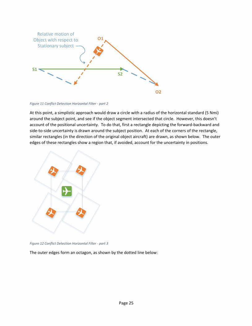
Figure 11 Conflict Detection Horizontal Filter - part 2
At this point, a simplistic approach would draw a circle with a radius of the horizontal standard (5 Nmi)
around the subject point, and see if the object segment intersected that circle. However, this doesn’t
account of the positional uncertainty. To do that, first a rectangle depicting the forward-backward and
side-to-side uncertainty is drawn around the subject position. At each of the corners of the rectangle,
similar rectangles (in the direction of the original object aircraft) are drawn, as shown below. The outer
edges of these rectangles show a region that, if avoided, account for the uncertainty in positions.
Figure 12 Conflict Detection Horizontal Filter - part 3
The outer edges form an octagon, as shown by the dotted line below:

Page 26
Figure 13 Conflict Detection Horizontal Filter - part 4
This region is expanded by the separation standard of 5 NMI:
Figure 14 Conflict Detection Horizontal Filter - part 5
Finally, to evaluate the possible conflict, we see if the relative object segment (with respect to the
stationary subject segment) intersections this outer octagon:

Page 27
Figure 15 Conflict Detection Horizontal Filter - part 6
In this example, we would have a conflict, starting at where O1-O2 first intersects the octagon and
ending where it exits the octagon at the bottom of the figure.
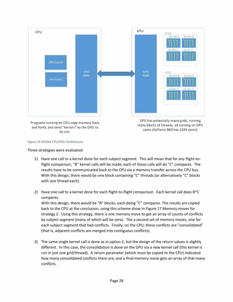
4.5.3 Parallelization Strategies Given this basic algorithm, the challenge in using the GPU is what kind of memory transfers are done
between CPU and GPU (and back), and how much work is done by each “subroutine” (or kernel, in
NVIDIA’s documentation). Figure 16 NVIDIA CPU/GPU Architecture shows the basic architecture of
NVIDIA’s GPU display boards existing in a desktop PC. The conflict detection kernel that compares one
segment to another segment is part of program structures that will eventually do A*B*C compares,
where “A” is the total number of flights in the airspace, “B” is the average number of segments in the
newly-introduced flight (the subject flight) and “C” is the average number of segments in the existing
(object) flights. B and C are equal, so if we confine ourselves to one flight-to-flight compare, the
problem includes B*C comparisons.
Page 28
Figure 16 NVIDIA CPU/GPU Architecture
Three strategies were evaluated:
1) Have one call to a kernel done for each subject segment. This will mean that for any flight-to-
flight comparison, “B” kernel calls will be made; each of those calls will do “C” compares. The
results have to be communicated back to the CPU via a memory transfer across the CPU bus.
With this design, there would be one block containing “C” threads (or alternatively “C” blocks
with one thread each).
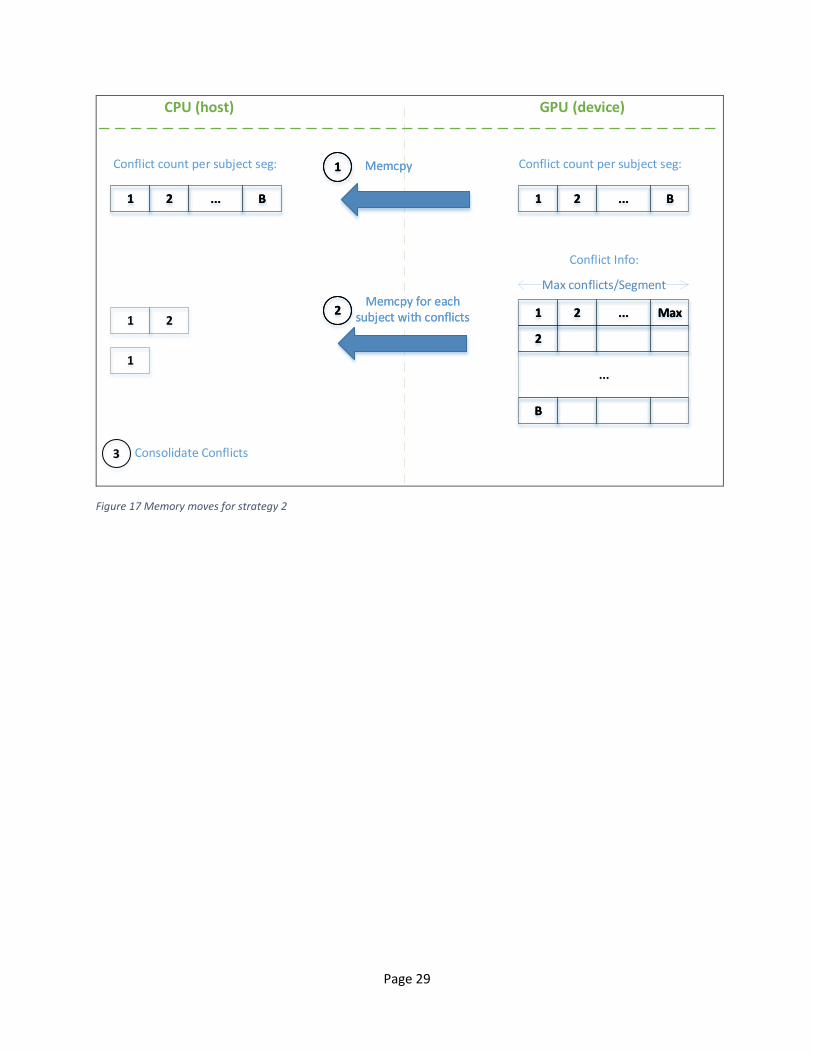
2) Have one call to a kernel done for each flight-to-flight comparison. Each kernel call does B*C
compares.
With this design, there would be “B” blocks, each doing “C” compares. The results are copied
back to the CPU at the conclusion, using this scheme show in Figure 17 Memory moves for
strategy 2. Using this strategy, there is one memory move to get an array of counts of conflicts
by subject segment (many of which will be zero). The a second set of memory moves, one for
each subject segment that had conflicts. Finally, on the CPU, these conflicts are “consolidated”
(that is, adjacent conflicts are merged into contiguous conflicts).
3) The same single kernel call is done as in option 2, but the design of the return values is slightly
different. In this case, the consolidation is done on the GPU via a new kernel call (this kernel is
run in just one grid/thread). A return parameter (which must be copied to the CPU) indicated
how many consolidated conflicts there are, and a final memory move gets an array of that many
conflicts.
Page 29
1 2 ... B1 2 ... B 1 2 ... B1 2 ... B
1 2 ... Max1 2 ... Max
22
BB
...
Max conflicts/Segment
Conflict count per subject seg:Conflict count per subject seg:
Conflict Info:
1 2
1
3 Consolidate Conflicts
1 Memcpy1 Memcpy
2Memcpy for each
subject with conflicts2
Memcpy for each subject with conflicts
CPU (host) GPU (device)
Figure 17 Memory moves for strategy 2

Page 30
1 2 ... B1 2 ... B
Conflict count per subject seg:
1
CPU (host) GPU (device)
1 2 ... Max1 2 ... Max
1 2 ... Max1 2 ... Max
22
BB
...
Max conflicts/Segment
Conflict Info:
1 2 ... Max
2
B
...
Max conflicts/Segment
Conflict Info:
1Kernel call to
consolidate conflicts1
Kernel call to consolidate conflicts
Memcpy to get count of conflicts
2Memcpy to get
count of conflicts2
Memcpy of consolidated conflicts
3Memcpy of
consolidated conflicts3
1 2 ... Max1 2 ... Max
Figure 18 Memory moves for strategy 3

Page 31
5 Implementation Trajectory generation, Use of Forecasted Data and Wind Optimal Trajectories are implemented using
the Python language. It offers the following advantages:
• Portable to many operating systems.
• Has the concepts of exception handling, classes, objects, modules, and packages.
• Has a wealth of other packages for scientific computing.
In spite of not being strongly typed or compiled before execution, this makes Python attractive for this
effort.
For an IDE, the PyDev Eclipse plug-in [11] is used. Git [12] is used for configuration management.
Python offers some limited documentation support in the language, but a separate design document is
among the deliverables; this will discuss major code structure and design decisions.
The development platform is a personal computer (desktop). Tests will also be run on this
configuration.
The parallel processing experiment utilizes the processing features of a Graphics Processing Unit (GPU).
A sequential implementation is compared to the parallel implementation. For this experiment, the C
language is chosen. In order to fairly compare running the algorithm sequentially vs. in a parallel
configuration, the same language has to be used in both cases. Since the GPU must be programmed in C
(even if a different language is used to express the algorithm, it will ultimately get converted to C code
to run on the GPU), C is chosen for the CPU as well.
This is run on a desktop PC running windows, with an Nvidia GEFORCE 960 graphics card. The CPU has
multiple cores, but only core is used for the sequential version. The desktop processor has Intel i7-6700
processors with 4 cores and a clock speed of 3.40 GHz. The GEFORCE 960 has 8 floating point processors
with a clock speeds of 1.1 GHz.
6 Validation Methods The experiments that use a trajectory will be validated through careful construction of test cases (using
alternative computations to ensure the necessary conditions are created), and then running those test
cases to be sure the desired result is obtained.
The basis for all this work is a valid trajectory. Trajectory verification occurs on two levels, and takes
advantage of the fact that a known, proven implementation exists (from real air traffic control (ATC)
systems). First, the low level equations for thrust, drag, etc., are verified against existing
implementations of those equations (same inputs should produce the same outputs). Second, the
overall trajectory that was generated is compared against a similar result from an ATC system simulator.
This overall comparison for a descent segment is shown in Figure 19.

Page 32
Figure 19 Trajectory Generation Comparison
There are two places where there are noticeable differences:
1) At the top of descent, both cases shown a period of acceleration, during which the desired
descent speed is attained (this speed is different than the cruise speed of the aircraft, requiring
this period of acceleration). During this period, the rate of descent will be smaller than normal,
because energy is being used to change the speed. The Python generated trajectory ends this
period sooner than the ATC version. A detailed analysis was undertaken for this; it revealed a
bug in the ATC code (wrong value for acceleration was being used).
2) The Python generated trajectory ends sooner than the ATC trajectory. This is simply a function
of the flight intent; the flight chosen for generation in Python was destined for an airport at 285
feet above sea level; the ATC flight was going to an airport at 14 feet above sea level. Hence the
Python trajectory ends sooner.
The above comparison is done without any wind (in order to have a valid comparison, wind data must
be equal, and there is no way to use the same wind conditions in both cases). Another test is needed to
show that the wind speeds are applied properly. For this, a "windy" day was chosen, where there was a
significant head wind in the Python flight’s direction. This is expected to slow down the aircraft.
0
5000
10000
15000
20000
25000
30000
35000
40000
80 100 120 140 160 180 200
Alt
itu
de
(Fe
et)
Along Route Distance (NMI)
Python Implementation vs. ATC ImplementationBoeing B735 - Cruise alt 35,000
ATC
Python

Page 33
Figure 20 Effect of Wind on Trajectories
In both plots, the blue line is the trajectory with the head wind applied; the red line shows the same
flight without wind. In an altitude vs. time plot, the climb and descent portions are identical (since the
calculation of rate of climb/descent (Equation 4-5.4) does not depend on ground speed, only true
airspeed. However, in this case, the cruise segment is elongated by more than 6 minutes due to the
head wind. The same information presented as an altitude vs. distance plot shows the flight is at cruise
for a longer distance, as the ground speed at cruise is reduced by the head wind.
7 Test Problems for Verification
7.1 Use of Weather Forecast Models Several months of real weather models has been obtained from NOAA. Starting with the same flight
intent input, several trajectories are generated using both the current forecast only and the future
forecasts. These trajectories are chosen to traverse the FIR in different directions, in order to
experience head and tail winds (see Figure 5 Flights Paths for the Use of Forecasted Weather analysis).
The total flight time of each flight will be compared.
7.2 Wind Optimal Trajectories Using both the weather models used above and synthetic models designed to have greatly varying wind
speeds in different regions, the Particle Swarm Optimization techniques will be used on a single flight.
7.3 Parallelizing Conflict Detection An entire set of flights, as typically would be found in a FIR, is not needed for this experiment. Rather,
we just need pairs of flights that show various degrees of “closeness” to being in conflict with one
another. These are run through both a sequential algorithm and the parallel algorithm. Conflicts
detected should be identical, and processing times can be compared. Since we are measuring both CPU
and GPU time, the same experiment was run many times and wall clock time from beginning to end was
compared.
0
10000
20000
30000
40000
0 20 40 60
Alt
itu
de
(fe
et)
Time (minutes)
Altitude vs. Time
0
10000
20000
30000
40000
0 100 200 300 400Alt
itu
de
(fe
et)
Along Route Distance (NMI)
Altitude vs. Distance
Page 34
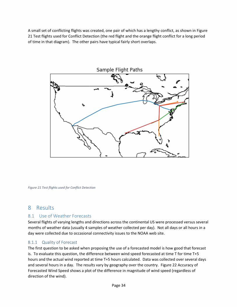
A small set of conflicting flights was created, one pair of which has a lengthy conflict, as shown in Figure
21 Test flights used for Conflict Detection (the red flight and the orange flight conflict for a long period
of time in that diagram). The other pairs have typical fairly short overlaps.
Figure 21 Test flights used for Conflict Detection
8 Results
8.1 Use of Weather Forecasts Several flights of varying lengths and directions across the continental US were processed versus several
months of weather data (usually 4 samples of weather collected per day). Not all days or all hours in a
day were collected due to occasional connectivity issues to the NOAA web site.
8.1.1 Quality of Forecast The first question to be asked when proposing the use of a forecasted model is how good that forecast
is. To evaluate this question, the difference between wind speed forecasted at time T for time T+5
hours and the actual wind reported at time T+5 hours calculated. Data was collected over several days
and several hours in a day. The results vary by geography over the country. Figure 22 Accuracy of
Forecasted Wind Speed shows a plot of the difference in magnitude of wind speed (regardless of
direction of the wind).

Page 35
Figure 22 Accuracy of Forecasted Wind Speed
The upper northwest has the least accurate forecasts, probably due to the relatively fewer number of
sensors in that area.
A flight traveling across country, with a continuous error of 3 knots in typical cruise speed of 420 knots
would be 2 minutes off in total flight time. In practice, however, these errors aren’t continuous, and in
some cases cancel each other out (some forecasts are too fast, some are too slow). In addition, flights
rarely fly directly into a headwind or ahead of a tail wind. Analysis of the data shows that the forecast
error accounts for at most 0.2 minutes of flight time, which is acceptable when we are looking for
differences of two to three minutes.
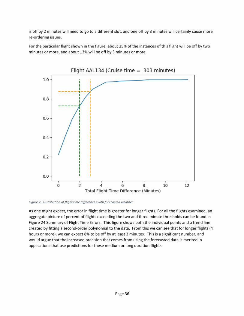
8.1.2 Impact on Flight Time Each flight in our set was analyzed against more than 400 weather samples. For each flight, results such
as shown in Figure 23 Distribution of flight time differences with forecasted weather is obtained, which
shows, for this one flight, the percentage of flights that are different by a particular amount. Two points
are highlighted; a difference of 2 minutes and a difference of 3 minutes. The scheduling of flights is
done in “slots” of one minute in duration. For the busiest airports, these slots are scheduled to be full,
so an error big enough to move to a different slot will cause scheduling problems (the schedule will have
to be adjusted in real time by having flights speed up, slow down or go into hold patterns). A flight that
Page 36
is off by 2 minutes will need to go to a different slot, and one off by 3 minutes will certainly cause more
re-ordering issues.
For the particular flight shown in the figure, about 25% of the instances of this flight will be off by two
minutes or more, and about 13% will be off by 3 minutes or more.
Figure 23 Distribution of flight time differences with forecasted weather
As one might expect, the error in flight time is greater for longer flights. For all the flights examined, an
aggregate picture of percent of flights exceeding the two and three minute thresholds can be found in
Figure 24 Summary of Flight Time Errors. This figure shows both the individual points and a trend line
created by fitting a second-order polynomial to the data. From this we can see that for longer flights (4
hours or more), we can expect 8% to be off by at least 3 minutes. This is a significant number, and
would argue that the increased precision that comes from using the forecasted data is merited in
applications that use predictions for these medium or long duration flights.

Page 37
Figure 24 Summary of Flight Time Errors
8.2 Wind Optimal Trajectories Optimal wind-aided trajectories should find “less expensive” trajectories than the nominal case. The
reduction in expense can be quantified. In addition, examining some real NOAA data can show how
likely it is that alternate, less expensive routes can be found.
8.3 Parallel Processing As each scheme was coded, it was measured and compared against the same processing being done
strictly in the CPU. The flight and conflict characteristics of the flights in conflict are summarized here:
Subject Segs (B) Object Segs (C) B x C Subject Segs in Conflict Seg Pairs in Conflict
137 154 21098 1 2
174 137 23838 4 8
174 154 26796 27 52
137 222 30414 0 0
222 154 34188 2 4
174 222 38628 2 4
Scheme 1, which made one kernel call for each subject segment, is compared against a CPU-only
solution:

Page 38
In this scheme, the kernel invocation overhead dominates and the GPU version performs much worse
that the CPU only version.
Schemes 2 and 3 reduce that kernel overhead by making just one call to do all comparisons:
0
5
10
15
20
25
30
35
40
45
20000 25000 30000 35000 40000
Elap
sed
TIm
e (
mill
ise
con
ds)
Number of Comparisons (B x C)
Conflict Detection on CPU vs. GPU - Scheme 1
CPU
GPU1

Page 39
The CPU line shows a fairly linear relationship between the number of comparisons and run time.
Schemes 2 and 3 have generally reduced the time to below what is achievable on the CPU, except for
the case with 26,796 comparisons. This is the case where there are many segments in conflicts. Scheme
2 will therefore do many array copies from GPU to CPU, and that copy overhead spikes the execution
time.
Scheme 3 moderates that overhead at the expense of a small amount of processing on the GPU for
conflict consolidation.
The GPU execution time also is growing with a flatter slope than the CPU scheme, probably because it
can better interleave short kernel executions with longer ones, while we are only using one core, and
hence one instruction pipeline, on the CPU.
Future work could serve to lower the GPU numbers more, by perhaps running all A*B*C comparisons
with one kernel call (utilizing several more grids) or perhaps using faster memory in the GPU (the GPU
has several difference classes of memory, all but the most general is limited in size or scope, and the
fastest is limited to being read-only in the GPU).
0
0.5
1
1.5
2
2.5
3
3.5
20000 22000 24000 26000 28000 30000 32000 34000 36000 38000 40000
Elap
sed
Tim
e (
mill
ise
con
ds)
Number of Comparisons (B x C)
Conflict Detection on CPU vs. GPU - Schemes 2 and 3
CPU
Scheme 2
Scheme 3

Page 40
9 Conclusion The creation of a framework to produce trajectories, given the parameters found in a BADA dataset, can
be used for many experiments of interest to ATC. This project established that framework and
conducted a few such experiments. These experiments were designed to provide insight into situations
confronting ATC today, and the framework can continue to be used for future work.
The primary benefit was to establish the framework and show experiments can effectively use it.
The “Use of Forecasted Weather” experiment has shown that for flights of longer than 3 hours,
forecasted weather will improve the estimates of arrival at the destination meter fix by enough that it
should be used; Figure 24 Summary of Flight Time Errors shows that 10% of flights of 3 hours or more
will be off by at least 2 minutes.
The “Wind Optimal Trajectories” experiment shows that, for light aircraft such as unmanned aerial
vehicles (drones), where the aircraft’s speed is not much greater than the fastest wind speed
encountered, a wind optimal trajectory can save significant time. The method presented is a compute-
efficient way to find those trajectories.
Finally, the “Parallel Conflict Probe” experiment shows that performance gains can be had by running
parts of the conflict probe algorithm on the multiple cores in a GPU, and the CUDA framework provides
a straight-forward way to do that.
Appendix A. Timeline
Table 1 Proposed Schedule
Timeframe Progress Achieved
Thanksgiving Implement trajectory generation using BADA version 3 - completed Detail the particle swarm optimization algorithm to be used - completed
December Implement and measure the use of forecasted weather- completed
January Initial PSO algorithm for wind-aided trajectories- completed
February Initial parallel conflict detection algorithm- completed
March Additional parallel algorithm tests, tuning PSO algorithm- completed
May Final algorithms and analysis, produce final report- completed
If time allows Implement BADA 4, compare BADA 3 vs 4 – not attempted
Appendix B. Milestones The milestones roughly follow the schedule presented, including these items:
1) Basic Trajectory Generation algorithm implemented and tested
2) Initial version of each algorithm implemented
3) Final version of each algorithm implemented and tested

Page 41
4) Final report produced
Appendix C. Deliverables 1) Python/C Source Code, with comments
2) Design documentation to augment commented code
3) Results
4) Class presentations and reports
5) Draft papers, to be presented at the DASC conference in September 2017
Appendix D. Bibliography
1. Eurocontrol Base of Aircraft Data (BADA), http://www.eurocontrol.int/services/bada
2. “World Geodetic System – 1984”, www.unoosa.org/pdf/icg/2012/template/WGS_84.pdf
3. Aircraft Modelling Standards for Future ATC Systems; EUROCONTROL Division E1, Document No. 872003
4. Kennedy, J. and Eberhart, R. C. Particle swarm optimization. Proc. IEEE int'l conf. on neural networks Vol. IV, pp. 1942-1948. IEEE service center, Piscataway, NJ, 1995.
5. http://www.swarmintelligence.org/tutorials.php
6. GRid in Binary (GRIB), the World Meteorological Organization (WMO) Standard for Gridded Data, http://dao.gsfc.nasa.gov/data_stuff/formatPages/GRIB.html
7. “ERAM Conflict Management, Off-Line Problem Determination, and Utility Algorithms”, FAA document FAA-ERAM-2008-0423
8. “ERAM Flight Data Processing (FDP) and Weather Data Processing (WDP) Algorithms”, FAA document FAA-ERAM-2006-0045
9. “Filghtaware – Flight Tracking/Flight Status”, flightaware.com
10. National Digital Forecast Database GRID2 Decoder, https://www.weather.gov/mdl/degrib_home
11. Python IDE for Eclipse, http://www.pydev.org
12. Git fast version control, https://git-scm.com
13. “CUDA By Example”, Sanders and Kandrot
14. “CUDA C Programming Guide”, Nvidia Corporation
Appendix E. List of Abbreviations ARD Along Route Distance
ASDI Aircraft Display for Industry
ATC Air Traffic Control
BADA Base of Aircraft Data
CAS Calibrated Air Speed
CPU Central Processing Unit

Page 42
CSV Comma Separated Values, a file format
FAA Federal Aviation Administration
FIR Flight Information Region
GPS Global Positioning System
GPU Graphics Processing Unit
GRIB Grid in Binary
IDE Integrated Development Environment
ISA International Standard Atmosphere
NMI Nautical Miles
NOAA National Oceanic and Atmospheric Administration
ODE Ordinary Differential Equation
PSO Particle Swarm Optimization
ROCD Rate of Climb or Descent
TAS True Air Speed
TOD Top Of Descent
WGS World Geodetic System