a formalization of termination techniques in...
TRANSCRIPT

University of Innsbruck Institute of Computer Science
Cumulative Habilitation Thesis
A Formalization of TerminationTechniques in Isabelle/HOL
Rene Thiemann
January 21, 2013


fur Karin, Hannah und Jonas


Contents
I. Preface 3
1. Introduction 5
2. Major Problems 7
3. Related Work 11
4. Contributions 134.1. Certification of Termination Proofs using CeTA (Chapter 6) . . . . . . . . . 134.2. Certified Subterm Criterion and Certified Usable Rules (Chapter 7) . . . . 154.3. Signature Extensions Preserve Termination – An Alternative Proof via De-
pendency Pairs (Chapter 8) . . . . . . . . . . . . . . . . . . . . . . . . . . 164.4. Modular and Certified Semantic Labeling and Unlabeling (Chapter 9) . . . 184.5. Termination of Isabelle Functions via Termination of Rewriting (Chapter 10) 194.6. Generalized and Formalized Uncurrying (Chapter 11) . . . . . . . . . . . . 204.7. On the Formalization of Termination Techniques Based on Multiset Order-
ings (Chapter 12) . . . . . . . . . . . . . . . . . . . . . . . . . . . . . . . . 214.8. Certification of Nontermination Proofs (Chapter 13) . . . . . . . . . . . . . 224.9. Further Contributions . . . . . . . . . . . . . . . . . . . . . . . . . . . . . 244.10. Summary of Contributions . . . . . . . . . . . . . . . . . . . . . . . . . . . 24
5. Future Research 27
II. Selected Papers 29
6. Certification of Termination Proofs using CeTA 316.1. Introduction . . . . . . . . . . . . . . . . . . . . . . . . . . . . . . . . . . . 316.2. Formalizing Term Rewriting . . . . . . . . . . . . . . . . . . . . . . . . . . 336.3. Certifying Dependency Pairs . . . . . . . . . . . . . . . . . . . . . . . . . . 346.4. Certifying the Dependency Graph Processor . . . . . . . . . . . . . . . . . 36
6.4.1. Certifying Graph Decompositions . . . . . . . . . . . . . . . . . . . 376.4.2. Certifying Dependency Graph Estimations . . . . . . . . . . . . . . 386.4.3. Certifying Dependency Graph Decomposition . . . . . . . . . . . . 41
6.5. Certifying the Reduction Pair Processor . . . . . . . . . . . . . . . . . . . 416.6. Certifying the Whole Proof Tree . . . . . . . . . . . . . . . . . . . . . . . . 426.7. Error Messages . . . . . . . . . . . . . . . . . . . . . . . . . . . . . . . . . 446.8. Experiments and Conclusion . . . . . . . . . . . . . . . . . . . . . . . . . . 44

VI Contents
7. Certified Subterm Criterion and Certified Usable Rules 477.1. Introduction . . . . . . . . . . . . . . . . . . . . . . . . . . . . . . . . . . . 477.2. Preliminaries . . . . . . . . . . . . . . . . . . . . . . . . . . . . . . . . . . 497.3. The Subterm Criterion . . . . . . . . . . . . . . . . . . . . . . . . . . . . . 507.4. Usable Rules . . . . . . . . . . . . . . . . . . . . . . . . . . . . . . . . . . 537.5. Experiments . . . . . . . . . . . . . . . . . . . . . . . . . . . . . . . . . . . 607.6. Conclusion . . . . . . . . . . . . . . . . . . . . . . . . . . . . . . . . . . . . 62
8. Signature Extensions Preserve Termination 638.1. Introduction . . . . . . . . . . . . . . . . . . . . . . . . . . . . . . . . . . . 638.2. Preliminaries . . . . . . . . . . . . . . . . . . . . . . . . . . . . . . . . . . 658.3. Dependency Pairs . . . . . . . . . . . . . . . . . . . . . . . . . . . . . . . . 668.4. Main Results . . . . . . . . . . . . . . . . . . . . . . . . . . . . . . . . . . 678.5. Applications . . . . . . . . . . . . . . . . . . . . . . . . . . . . . . . . . . 698.6. Conclusion . . . . . . . . . . . . . . . . . . . . . . . . . . . . . . . . . . . . 75
9. Modular and Certified Semantic Labeling and Unlabeling 779.1. Introduction . . . . . . . . . . . . . . . . . . . . . . . . . . . . . . . . . . . 779.2. Preliminaries . . . . . . . . . . . . . . . . . . . . . . . . . . . . . . . . . . 78
9.2.1. Term Rewriting . . . . . . . . . . . . . . . . . . . . . . . . . . . . . 789.2.2. Semantic Labeling . . . . . . . . . . . . . . . . . . . . . . . . . . . 79
9.3. Modular Semantic Labeling and Unlabeling . . . . . . . . . . . . . . . . . 809.4. Dependency Pair Framework . . . . . . . . . . . . . . . . . . . . . . . . . . 869.5. Problems in Certification . . . . . . . . . . . . . . . . . . . . . . . . . . . . 909.6. Experiments . . . . . . . . . . . . . . . . . . . . . . . . . . . . . . . . . . . 929.7. Conclusion . . . . . . . . . . . . . . . . . . . . . . . . . . . . . . . . . . . . 92
10.Termination of Isabelle Functions via Termination of Rewriting 9510.1. Introduction . . . . . . . . . . . . . . . . . . . . . . . . . . . . . . . . . . . 9510.2. Preliminaries . . . . . . . . . . . . . . . . . . . . . . . . . . . . . . . . . . 96
10.2.1. Higher-Order Logic . . . . . . . . . . . . . . . . . . . . . . . . . . . 9610.2.2. Supported Fragment . . . . . . . . . . . . . . . . . . . . . . . . . . 9710.2.3. Function Definitions by Well-Founded Recursion . . . . . . . . . . . 9810.2.4. IsaFoR - Term Rewriting Formalized in Isabelle/HOL . . . . . . . . 9910.2.5. Terminology and Notation . . . . . . . . . . . . . . . . . . . . . . . 99
10.3. The Reduction to Rewriting . . . . . . . . . . . . . . . . . . . . . . . . . . 10010.3.1. Encoding Expressions and Defining Equations . . . . . . . . . . . . 10010.3.2. Embedding Functions . . . . . . . . . . . . . . . . . . . . . . . . . . 10110.3.3. Rewrite Lemmas . . . . . . . . . . . . . . . . . . . . . . . . . . . . 10210.3.4. The Simulation Property . . . . . . . . . . . . . . . . . . . . . . . . 10210.3.5. Reduction of Termination Goals . . . . . . . . . . . . . . . . . . . . 10310.3.6. Proof of the Simulation Property . . . . . . . . . . . . . . . . . . . 105
10.4. Examples . . . . . . . . . . . . . . . . . . . . . . . . . . . . . . . . . . . . 10610.5. Extensions . . . . . . . . . . . . . . . . . . . . . . . . . . . . . . . . . . . . 10710.6. Conclusion . . . . . . . . . . . . . . . . . . . . . . . . . . . . . . . . . . . . 109
11.Generalized and Formalized Uncurrying 11111.1. Introduction . . . . . . . . . . . . . . . . . . . . . . . . . . . . . . . . . . . 11111.2. Preliminaries . . . . . . . . . . . . . . . . . . . . . . . . . . . . . . . . . . 112

Contents VII
11.3. Applicative Rewriting and Uncurrying . . . . . . . . . . . . . . . . . . . . 11211.4. Uncurrying in the Dependency Pair Framework . . . . . . . . . . . . . . . 11811.5. Heuristics and Experiments . . . . . . . . . . . . . . . . . . . . . . . . . . 12311.6. Conclusions . . . . . . . . . . . . . . . . . . . . . . . . . . . . . . . . . . . 125
12.Formalization of Termination Techniques Based on Multiset Orderings 12712.1. Introduction . . . . . . . . . . . . . . . . . . . . . . . . . . . . . . . . . . . 12712.2. Preliminaries . . . . . . . . . . . . . . . . . . . . . . . . . . . . . . . . . . 12912.3. Formalization of the Generalized Multiset Ordering . . . . . . . . . . . . . 13012.4. Multiset and Recursive Path Ordering . . . . . . . . . . . . . . . . . . . . 13212.5. SCNP Reduction Pairs . . . . . . . . . . . . . . . . . . . . . . . . . . . . . 13612.6. Certification Algorithms . . . . . . . . . . . . . . . . . . . . . . . . . . . . 14112.7. Summary . . . . . . . . . . . . . . . . . . . . . . . . . . . . . . . . . . . . 142
13.Certification of Nontermination Proofs 14313.1. Introduction . . . . . . . . . . . . . . . . . . . . . . . . . . . . . . . . . . . 14313.2. Preliminaries . . . . . . . . . . . . . . . . . . . . . . . . . . . . . . . . . . 14413.3. A Framework for Certifying Nontermination . . . . . . . . . . . . . . . . . 14513.4. Loops . . . . . . . . . . . . . . . . . . . . . . . . . . . . . . . . . . . . . . 14613.5. Formalization . . . . . . . . . . . . . . . . . . . . . . . . . . . . . . . . . . 14713.6. Conclusions . . . . . . . . . . . . . . . . . . . . . . . . . . . . . . . . . . . 156
Bibliography 159


Acknowledgements
Clearly, without an appropriate environment it would not have been possible to developthis thesis. Therefore, I want to express my gratitude to those people that made thisthesis possible.
First of all, I want to thank Aart Middeldorp for giving me the freedom to freely letme pursue my research interests in the last years, for his support in providing me withthe necessary equipment, and for many useful feedbacks.
Insbesondere mochte ich auch Christian Sternagel danken. Es war eine wunderbareZeit, jemanden vor Ort zu haben, mit dem man uber Isabelle diskutieren konnte undgemeinsam Ideen in Formalisierungen und Paper umsetzen konnte.
Mein Dank gilt auch Georg Moser. Besonders wahrend langen Isabelle Entwicklungenwar es eine Freude, durch ihn die Gedanken wieder frei zu bekommen: sei es durchkurze Exkurse in die Welt der Komplexitat, durch politische Diskussionen in SteeringCommittees, oder besonders durch den Austausch kurzer Anekdoten uber unsere Kleinen.
Of course, I’m also grateful to the whole Computational logic group for a pleasant andfriendly research environment.
Naturlich bin ich auch den Entwicklern der Terminierungs Tools AProVE und TTT2dankbar, insbesondere Bertram Felgenhauer, Carsten Fuhs, Christian Kuknat, ChristianSternagel, Fabian Emmes, und Harald Zankl: ohne deren Entwicklung der Beweisausgabeware keine Zertifizierung moglich gewesen.
I would also like to express my gratitude to the Isabelle community. Since I started towork with Isabelle, I always got useful feedback on my questions. Moreover, several recentdevelopments on Isabelle have been beneficial for this thesis, like the code generator, theIsabelle collection framework, partial functions, regexp, parallelization, and jedit. Here,special thanks go to Alexander Krauss, Andreas Lochbihler, Florian Haftmann, LukasBulwahn, Makarius Wenzel, Peter Lammich, and Tobias Nipkow.
Many thanks also goes to the Austrian Science Fund (FWF). They supported all theselected papers (within the projects P18763 and P22767-N13).
Schließlich mochte ich mich naturlich auch bei meiner Familie bedanken, insbesonderebei Karin: in ihr fand ich immer den so wichtigen Ausgleich, der mich von der sehrtechnischen Arbeit zuruck in die reale Welt fuhrte, und ich bekam immer Ruckhalt, selbstin Zeiten, wo ich nur wenig Zeit fur die Familie hatte.


Part I.
Preface


1. Introduction
Termination is the important property of a program that all computation paths producea result in finite time. Although undecidable in general, much work has been spent onautomated termination analysis. As a result, today there are a variety of powerful tools forautomatic termination analysis for various languages: e.g., there are AProVE [39], COSTA[1], Julia [93], Matchbox [106], Polytool [82], Terminator [24], and TTT2 [67]. Several ofthese tools are competing in the annual international termination competition1 where theaim is to automatically investigate termination and complexity of programs in differentlanguages, i.e., currently term rewriting, Prolog, Haskell, or Java.
Due to the complexity of the tools itself, it is obvious that there might be bugs inthe implementations leading to wrong answers. And indeed, nearly every year in thecompetition some bugs were spotted since two tools gave contradicting answers, e.g., byproviding a termination and a nontermination proof for the same program. Therefore,it has been identified as a key challenge to independently certify the correctness of thegenerated proofs. Due to the size of these proofs a manual inspection is infeasible andalso error-prone. However, it can be done using interactive theorem provers like Coq [11],Isabelle [84], and PVS [88]. These theorem provers are used to model various aspects ofmathematics, programming languages, etc. in a logical system and afterwards formallyverify desired properties.
As a result, since 2007 also certifiers have entered the termination competition.
• In the A3PAT project2 [21, 25], the tool CiME was extended by a feature thattransforms termination certificates into Coq scripts. These scripts can be checkedwith help of the underlying Coq library Coccinelle on rewriting.
• Similarly, in the CoLoR project3 [13], the tool Rainbow produces Coq-scripts forcertified termination proofs. It is based on CoLoR, the Coq Library on Rewritingand termination.
• CeTA (Certified Termination Analysis) with its underlying formalization IsaFoR (Is-abelle Formalization of Rewriting) is our own certifier which entered the competitionin 2009.
With the help of these three certifiers (which we abbreviate by CC for CiME + Coccinelle,RC for Rainbow + CoLoR, and CI for CeTA + IsaFoR), several implementation bugs havebeen revealed which previously remained undetected. Furthermore, the formalization ofthe termination techniques also discovered some flaws in pen-and-paper proofs which inat least one case invalidated the main theorem of a termination technique [97].
In this thesis, we report on our work in this area, i.e., the development of CeTA andIsaFoR. It is structured as follows. In Chapter 2 we illustrate four main problems when
1http://www.termination-portal.org/wiki/Termination_Competition2http://a3pat.ensiie.fr3http://color.inria.fr

6 Chapter 1. Introduction
trying to develop a certifier. Related work is addressed in Chapter 3. Our own con-tributions in this area are discussed in Chapter 4. Here, we also explain which part ofeach selected paper has been developed by the co-authors. Future work is addressed inChapter 5 which ends Part I of this thesis. Afterwards, in Part II the selected papers areprovided in chronological order.

2. Major Problems
In order to develop a certifier for termination proofs three tasks have to be performed.
(i) The definition of termination has to be formally specified.
(ii) Termination methods have to be formalized in some library of a theorem prover.
(iii) Starting from a given certificate, one has to reconstruct a formal termination proofusing the termination methods from the previous step.
Once, these tasks have been established, a possible workflow for getting certified ter-mination proofs is as follows, cf. Figure 2.1.
First, an untrusted termination tool is invoked which has to deliver the answer (ter-minating, nonterminating, don’t know) in combination with a certificate which has tocontain enough information to reconstruct a proof to validate the answer. As an example,the certificate might be an XML-document which states which termination techniqueshave been applied and how they have been parametrized.
Afterwards, one can start the reconstruction to obtain a formal proof script. In thisstep, one has to link the termination techniques in the certificate to those which havebeen formalized. Moreover, in the proof script several assertions have to be stated whichensure that the termination techniques are applied correctly.
Finally, the formal proof script must be checked within a proof assistant.In order to maximize the reliability of this certification workflow, one should use proof
assistants which are based on the LCF-approach [43, 45, 89], where all generated proofshave to be accepted by some small trusted kernel. In that way, one can be quite certainthat during proof checking only correct proofs are accepted. Moreover, for the majorproperties and definitions in the specification—which are termination and the rewriterelation in our case—one can try to prove that their formalization corresponds to variousalternative definitions that are present in the literature [5,100]. For example, we define therewrite relation as →R := {(C[`σ], C[rσ]) | `→ r ∈ R} where C ranges over all contextsand σ over all substitutions, and afterwards we prove that our definition is equivalent toanother standard definition of the rewrite relation: →R = {(t, t[rσ]p) | t|p = `σ, ` → r ∈R, p ∈ Pos(t)} where Pos(t) is the set of positions in t.
input answer + certificate proof script
accept/failure
termination
tool
proof
reconstruction
proof
checking
Figure 2.1.: workflow for certified termination proofs

8 Chapter 2. Major Problems
Although the reliability is quite high, we want to mention that there still remain certainrisks where we just have to trust the system: the logic of the proof assistant may beinconsistent, there may be bugs in the kernel of the proof assistant as well as in thecompiler / interpreter that is used to run the proof assistant, and there may be errorsin the operating-system and in the hardware, and the hardware may be damaged. Tominimize these risks, several projects have been performed. For example, with Milawaand Jitawa there is a verified theorem prover running in a verified Lisp runtime, i.e.,soundness of the theorem prover was proven down to x86 machine code [80]. And inanother impressive project, an operating-system kernel was proven to be sound [60].
Despite these risks, we believe that formalized proofs contain far less errors than thosewhich are checked by human—we leave it up to the reader to figure out a list of risks thatarise when proofs are solely checked by humans. But even if we trust formalized proofs,we have to establish all three tasks that have been mentioned above.
Whereas the first task is easily solved in our case—since the notions of termination andthe rewrite relation of a term rewrite system (TRS) are easily defined—the second taskis by far more challenging because of the following two major problems.
Problem 1: Formalize many termination techniques Termination tools for termrewriting use several incomparable termination techniques. And for each individual ter-mination technique, we require a fully formalized proof. Here, standard formalizationproblems may arise: proofs in papers can contain gaps and are often not sufficiently de-tailed (“w.l.o.g.”, “easy to see”, “by induction”, “we consider only the most interestingcase”, . . . ), they may be based on other nontrivial theorems (from Ramsey theory, fromgraph-theory, . . . ), they may use nontextual representations like diagrams, and they makeuse of intuitive arguments which are hard or tedious to describe formally (“we can easilyreorder this sequence as follows such that . . . ”). Moreover, we will encounter the problem,that many termination techniques are using completely different concepts in their sound-ness proofs: the proofs are based on syntactic criteria, graph theory, automata theory,algebra, combinatorics, etc.
Hence, to get formalized proofs, all gaps have to be filled, all background theories haveto be formalized, and one has to find a good formal model for all the concepts that areused in the proofs.
Problem 2: Combine termination techniques Even if individual termination tech-niques have been proven correct, for their combination we need a common semantics,such that all techniques are sound w.r.t. that semantics. For example, for the rewriterelation of a TRS luckily there is only one semantics. However, often termination proofsare performed using the notions of dependency pairs and chains, and here there are atleast two different versions of evaluation (chains and minimal chains) [3]. The problem isthat some termination techniques are only sound for chains whereas other require min-imal chains. Hence, checking proofs which utilize both kinds of termination techniquescannot be done without adaptation: one first has to find some notion of chain which iscompatible with all termination techniques.
When considering the third task—proof reconstruction—two additional problems arise.
Problem 3: Check application of termination techniques In principle, the certificatecontains all major proof steps, i.e., every termination technique that has been applied is

9
listed in the certificate in combination with its parameters. However, it must be checkedthat the technique has been applied correctly, which is a problem that may range fromeasy via complex to undecidable.
For example, some termination methods are based on simple syntactic criteria whichcan easily be checked, like the application of dependency pairs or the switch from full- toinnermost-termination for orthogonal TRSs. However, for the latter technique one canweaken orthogonality to locally confluent overlay TRSs [46]. In that case, checking thepreconditions becomes undecidable as local confluence is undecidable.
As another example, consider termination methods based on well-founded orders, likepolynomial orders [73], the lexicographic path order (LPO) [58], or the recursive pathorder (RPO) [27]. For these methods one has to provide an algorithm to check whethertwo terms are in relation. This problem is in P (for LPO) [71], NP-complete (for RPO),and undecidable for polynomial orders. In the latter case, sufficient decidable criteria likeabsolute positiveness [56] are used which are again easy to check. Of course, one mightenrich the certificates by providing more detailed evidence why two terms are in relation.Then checking can be done more efficiently, but the certificates easily become bulky andare harder to produce.
As a last example, we consider size-change termination which is a PSPACE-completeproblem [74]. Here, there is no chance to enlarge the certificate such that checking theproof can be done in polynomial time, unless PSPACE = NP. We shortly illustrate whyalso in practice an enlarged certificate is not helpful for this technique. One standardalgorithm to decide size-change termination works as follows. It computes a (possiblyexponentially large) closure of size-change graphs where one has to test that no badgraphs appear in this closure. In principle, one can add the closure to the certificate, butthis does not improve the situation, since checking that the provided closure is correcthas the same asymptotic complexity as computing the closure.
To summarize, we require methods to guarantee the correct application of terminationtechniques which is not always easy.
Problem 4: Obtaining certificates It is obvious, that for checking a termination proofwe require certificates from the tools. These certificates should be sufficiently detailedand in some machine readable format. However, when we started our work, each of thecertifiers had its own proof format with varying level of detail. Hence, for a terminationtool to support many certifier, the tool had to implement many proof printing procedures:one for each certifier. Putting this into another perspective, we had to convince the toolauthors to also support and integrate our proof format.
As a solution to this problem we developed a common proof format for certificates fortermination problems: the certification problem format (CPF).1 The CPF-format wasdesigned as a combination of all previously existing formats by several groups: membersfrom all three certifiers CC, RC, and CI contributed, as well as members from the termina-tion tools AProVE and TTT2. As a result, today termination tools only have to support oneoutput format (CPF) and then all three certifiers can be used to independently certify theanswer. Moreover, we also wrote pretty printer which transform CPF proofs into humanreadable proofs, so that the termination tool authors can also drop their human readableexport functionality for those parts of the proof that are covered by CPF.
1http://cl-informatik.uibk.ac.at/software/cpf/


3. Related Work
The alternative certifiers CC and RC clearly have the closest connection to our work.Moreover, there also is a PVS formalization on term rewriting, trs [34, 35]. It was notmentioned before, since as far as we know, it is currently not used for certification oftermination proofs.
Although all of the formalizations are on term rewriting there are several differenceswhich we will list in the remainder of this chapter.
Theorem Prover CI is based on Isabelle/HOL, CC and RC use Coq, and trs utilizesPVS. As a consequence, the proof of some result in IsaFoR can look quite different froma similar proof of the same result in one of the other formalizations. Moreover, there isno easy way to import or share theorems which have already been integrated in the otherformalizations. As a matter of fact, we are only aware that some results are shared amongthe Coq based formalizations Coccinelle and CoLoR.
Representation In CI everything is developed using a deep embedding, whereas in CCand RC also shallow embeddings are used. To shortly illustrate the difference betweendeep and shallow embedding, consider the following TRS R for subtraction:
minus(x, 0)→ x
minus(s(x), s(y))→ minus(x, y)
For certification, in both CC and RC first an inductive set or type for the signature iscreated on the fly within Coq (shallow), which contains exactly the three symbols minus,s, and 0. In CI however, there is no dedicated signature—minus, s, and 0 are just strings.Similarly, for solving arithmetic constraints which may arise from proving terminationof R by a polynomial interpretation, in CC the Coq tactic omega is invoked (shallow),whereas for CI an algorithm for solving these constraints has been formalized (deep).
Both designs have their own advantages: using a shallow embedding sometimes allowsfor more elegant formalizations since the builtin methods from the theorem prover can beused to adequately model or solve a problem; and with a deep embedding, the certificationalgorithms can also run outside the theorem prover and are less brittle to changes in thetheorem prover.
Support of termination techniques As we have focussed our work to develop a certifierwith a high coverage of termination technique for first order term rewriting, CI containsseveral techniques in this area which are not available in the other certifier.1 For example,during the latest full run of termination tools in 2011, where every participating tool wastested on every problem of the termination problem database, 3675 termination and
1See http://cl-informatik.uibk.ac.at/software/ceta/#introduction for the current list of tech-niques which are supported by CeTA.

12 Chapter 3. Related Work
nontermination proofs have been generated for TRSs.2 In this experiment, there havebeen dedicated termination tools to support both CI and CC, i.e., some termination toolsdelivered proofs which are known to be supported by CI and other tools delivered proofsespecially for CC. Whereas CC had to refuse 1694 proofs as they contained unsupportedtechniques, CeTA only had to refuse 525 proofs. And in the meantime, all 3675 proofs canbe certified using CeTA version 2.8. These numbers clearly demonstrate a high coverage ofCeTA in this area.
However, in other areas the picture is inverted: for example, IsaFoR does not containany result on higher-order rewriting, but CoLoR does [63].
2http://termcomp.uibk.ac.at/termcomp/competition/certificationResults.seam?cat=
10235&comp=260918

4. Contributions
In this chapter, we first explain how the selected papers in the second part of this thesiscontribute to solving the four mentioned problems. Here, the papers are listed in order oftheir publication date. Afterwards, we report on further work in the area of certification,which has been performed in IsaFoR but is not covered in the selected papers.
4.1. Certification of Termination Proofs using CeTA(Chapter 6)
Publication details
Rene Thiemann and Christian Sternagel. Certification of Termination Proofs using CeTA.In Proceedings of the 22nd International Conference on Theorem Proving in Higher OrderLogics, volume 5674 of LNCS, pages 452–468. Springer, 2009.
In this initial paper on IsaFoR and CeTA, we give details on our formalization of threeimportant termination techniques—dependency pairs, dependency graph decomposition,and reduction pairs—a clear contribution to Problem 1.
Note that all of these techniques are also supported by the other certifiers. Therefore,the real novelty in this paper is the approach of dealing with Problem 3. Both RC andCC use a mixture of three possibilities to generate proof scripts for a certificate: invokeexecutable functions which have been proven correct, perform on-the-fly generation ofproofs by untrusted tools, and call built-in solvers of the proof assistant. In contrast,for every termination technique in IsaFoR we always provide an executable function thatchecks the correct application—even for those techniques that compose other terminationtechniques.
As a consequence, there is also one check-function check-trs-termination-proof
which checks full proof trees. It takes a proof and a TRS as input and we have formallyproven its correctness: if check-trs-termination-proof R results in “OK” then ter-mination of R is guaranteed. Hence, our proof scripts are always identical, they justevaluate check-trs-termination-proof and demand that the result is “OK”.
This allows us to not generate a proof script at all. We can just invoke the codegenerator of Isabelle [49] to obtain check-trs-termination-proof as external program(Haskell, OCaml, SML, or Scala) which can then be compiled and executed. And this isexactly what CeTA is. It consists of a small hand written main function which reads a file,invokes check-trs-termination-proof on the input, and accepts the proof if the resultis “OK”, and otherwise throws an error-message. Hence, for checking proofs one does nothave to install and run Isabelle, but one can just compile CeTA and execute it like everyother program.

14 Chapter 4. Contributions
This design has several consequences:
• Since proof checking via CeTA is execution of native code, and does not run withinthe proof assistant, CeTA is usually faster than the other two certifiers. Moreover, itallows us to also integrate more time intensive termination techniques. For example,the dependency graph estimation EDG∗∗∗ (a combination of the estimations in [41]and [50]), and the termination techniques of semantic labeling [110] (Chapter 9),size-change termination [74], and matchbounds [36] all have complex applicationcriteria where the corresponding check-functions benefit from the speedup that isobtained from running native code.
• If a proof script is rejected, then one can immediately see where the proof is rejected.Depending on the structure of the proof script, it is then more or less easy to figureout which part of the termination proof was rejected. In contrast, if the result ofour check-trs-termination-proof function were just a Boolean, then it wouldnot be visible which part of the proof was rejected. Therefore, the return type ofour check-functions is a disjoint sum: either we return “OK”, or a string which isthe error message. Since all our check-functions provide detailed human readableerror messages, it is easy to figure out which part of the proof is not accepted andwhy it is not accepted, where it is not required to read any proof script at all. Inthe paper we further describe how readable error messages can be integrated intothe check-functions without becoming an overhead when proving soundness of thesefunctions.
• Since all our formal proofs are done statically (soundness of termination techniquesand soundness of check-functions), we are quite robust against any changes in theproof assistant. With every new release of the proof assistant, we just have toreplay all our proofs and immediately detect problems which are due to changes inthe proof assistant—which can then be easily fixed. However, CeTA will be the sameprogram as before (unless there are severe changes in the code generator), so thechanges in the proof assistant will have no impact on checking the certificates. Incontrast, if we would have generated proof scripts on the fly, then some problemsmay occur only during certification which are not visible when replaying the proofsfor the theorems in the library.
• As all our check-functions have to be fully executable, they cannot make use ofinternal tactics, solvers, etc., which might be available in the proof assistant. Hence,it is more tedious to develop these checks, as most parts have to be developedfrom scratch. Moreover, our design requires that the full formalization is deeplyembedded, so we cannot model parts of term rewriting by the builtin constructs ofthe proof assistant as it is done in both RC and CC.
To summarize, in this paper we formalized well known termination criteria, and pre-sented a new approach to certify termination proofs via code generation. Here, my con-tributions are the formalization of EDG∗∗∗, polynomial orders, and the idea of usingcode generation and error messages. My co-author formalized dependency pairs and theunderlying theory on abstract reduction systems and term rewrite systems.

4.2. Certified Subterm Criterion and Certified Usable Rules (Chapter 7) 15
4.2. Certified Subterm Criterion and Certified UsableRules (Chapter 7)
Publication details
Christian Sternagel and Rene Thiemann. Certified Subterm Criterion and Certified Us-able Rules. In Proceedings of the 21st International Conference on Rewriting Techniquesand Applications, volume 6 of LIPIcs, pages 325–340. Schloss Dagstuhl – Leibniz-Zentrumfur Informatik, 2010.
This paper is mainly devoted to Problem 1, the formalization of important terminationtechniques. In the following, we will concentrate on the formalization of usable rules[3, 41, 42] since my co-author developed the part about the subterm criterion [51].
Note that as for the estimation of the dependency graph, there are various definitions ofusable rules. To be able to certify many termination proofs we integrated one of the mostpowerful versions of usable rules, namely the one in [41] which additionally is combinedwith argument filters as in [42]. Here, we tried to generalize as much as possible.
One of the main results is easily stated where the exact definitions can be seen inChapter 7: if R is finite, (P ,R) is a dependency pair problem, (%,�) is a reductionpair compatible with an argument filter π, U are the usable rules of (P ,R) w.r.t. π, andP ∪ U ∪ Cε ⊆ %, then for a termination proof it is allowed to delete all pairs s→ t fromP which are strictly decreasing, i.e., which satisfy s � t.
Although this seems exactly like the statement that is given in literature, we want toillustrate that our formalization contains something more general:
• We do not require that R is a well-formed TRS, i.e., that for every rule `→ r ∈ Rthe left-hand side ` must not be a variable and that all variables of r also occur in `.As a consequence during certification we do not have to check for well-formednesswhen applying this techniques. However, it complicates the soundness proof of thistermination technique, as it relies upon the fact that →R is finitely branching, butnon-well-formed TRSs may be infinitely branching.
• We do not make any assumption on the set of variables or function symbols, sothat this technique can be applied for every type of variables and function sym-bols, even for degenerated cases. As an example consider the TRS Cε which inthe literature is defined as Cε = {c(x, y) → x, c(x, y) → y} which can be used tomake nondeterministic choices. Now let the set of variables be a singleton set, i.e.x = y. Then there is no choice anymore and the proof would fail. Therefore, inthe formalization we define Cε :=
⋃s,t{c(s, t) → s, c(s, t) → t} where s and t range
over all terms. With this definition we can prove the result, and moreover, when-ever {c(x, y) → x, c(x, y) → y} ⊆ %, then also Cε ⊆ % since % is required to beclosed under substitutions. Hence, we do not impose any additional constraint onthe reduction pairs that can be used.
Besides these generalizations, the paper illustrates a nice trick to avoid the developmentof a working list algorithm to compute the usable rules: The usable rules are usuallydefined via some inductive definition, i.e., they are the least set U ⊆ R such that someproperty P on U is satisfied. Although a standard working list algorithm for computingthe usable rules is easily written, it would require a tedious proof to show termination

16 Chapter 4. Contributions
of the algorithm, and of course, one would require proofs for soundness and correctness.In contrast, if the usable rules are provided in the certificate, then one just has to checkwhether they satisfy property P : it is not at all essential, that the given set of rules isindeed the least set satisfying P .
Note that requiring the usable rules in the certificate is not a severe burden for thetermination tools,1 since they will have to compute the usable rules in any case. Moreover,providing the usable rules in the certificate has the advantage, that one can also showthis information when pretty printing the certificate into a human readable format.
To summarize, in this paper we formalized two important termination techniques andgeneralized them, such that less preconditions have to checked during certification. More-over, we illustrated how to completely avoid the formalization of a working list algorithmto compute an inductively defined set.
4.3. Signature Extensions Preserve Termination – AnAlternative Proof via Dependency Pairs (Chapter 8)
Publication details
Christian Sternagel and Rene Thiemann. Signature Extensions Preserve Termination –An Alternative Proof via Dependency Pairs. In Proceedings of the 19th Annual Confer-ence of the EACSL on Computer Science Logic, volume 6247 of LNCS, pages 514–528.Springer, 2010.
Assume that some property P can be proven for all terms over the signature F whereF are all those symbols that appear in the TRS R. Now consider an extended signatureF ′ ⊇ F . The question of signature extensions is the question for which properties P wecan conclude that P also holds for all terms over F ′.
It is a well-known result that signature extensions are sound for termination and thisfact is also used in termination tools which is illustrated in the following example.
Example 4.1. Let R consist of the following rules, and let F = {a, b, f}.
a(b(b(x)))→ a(b(a(a(a(a(x)))))) (1)
f(x, y)→ x (2)
f(x, y)→ y (3)
Using an polynomial order it is possible to remove rules (2) and (3), and it remains toprove termination of R′ = {(1)} for all terms over the signature F . Using the result ofsignature extensions it suffices to prove termination of R′ w.r.t. the signature F ′ = {a, b}.Since in F ′ every symbol is unary, one can interpret the terms as strings and apply stringreversal which results in
b(b(a(x)))→ a(a(a(a(b(a(x)))))).
Afterwards there are no dependency pairs and termination is trivially proven.Without the result on signature extensions, one would not be able to apply string
reversal, and a more complex proof would be required to prove termination of R′ over F .
1In the meantime, IsaFoR also contains an algorithm to compute the usable rules. It was developed forother termination techniques where the computation of usable rules occurs as a side-problem, andwhere adding the usable rules to the certificates would make the certificates too bulky.

4.3. Signature Extensions Preserve Termination – An Alternative Proof viaDependency Pairs (Chapter 8) 17
In the paper there are essentially three contributions:
(i) There is a new formalized proof that signature extensions are sound for termina-tion, which is simpler than existing proofs. It just requires that signature extensionsare sound when considering chains of dependency pairs, which can be proven in astraight-forward way. And using this result in combination with soundness and com-pleteness of dependency pairs already suffices to establish the signature extensionresult.
(ii) A counter-example is provided which proves that signature extensions are unsoundwhen considering minimal chains of dependency pairs.
(iii) It is shown that under the additional assumption of left-linearity signature exten-sions are sound for minimal chains.
Especially Contributions (ii) and (iii) are important: In at least two papers [53, 95]signature extensions are used in combination with minimal chains—taking this unsoundresult for granted. Luckily, in case of uncurrying [53], the major result is still valid(cf. Chapter 11). In contrast, for root-labeling [95] we were able to also construct acounter-example showing that without further restrictions, root-labeling is unsound whenconsidering minimal chains. Hence, Contribution (iii) was important since it allows touse root-labeling at least for left-linear TRSs.
As a consequence, termination tools like AProVE and TTT2 now require left-linearity ifthey want to apply root-labeling when using dependency pairs.
Clearly this paper contributes to Problem 1, as now termination techniques such asstring reversal can be certified, however, it shows the overall relevance of formalization, aswe have refuted the soundness of an existing termination technique in theory and practice.
Whereas most of the formalization for this paper was mainly done by my co-author, Ideveloped the counter-examples for both signature extensions and root-labeling. Both ofus were involved in the process of finding the alternative proof for signature extensions viadependency pairs and in the process of developing a fix for minimal chains—in the formof the additional requirement of left-linearity. Note that in the meantime, I extended thework on signature extensions by integrating the following facts in IsaFoR.
• Signature extensions are sound for innermost rewriting, no matter whether oneconsiders termination of TRSs, chains, or minimal chains.
• Signature extensions are sound for relative termination of R modulo S2 if S iswell-formed.
• In general, signature extensions are unsound for relative termination. For the TRSsR = {a → b} and S = {a → x}, we have relative termination of R modulo S ifwe consider terms over the signature F = {a, b}, but for the extended signatureF ∪ {f} where f is a binary symbol, relative termination does no longer hold: a→Sf(a, a)→R f(a, b) = C[a]→S C[f(a, a)]→R . . . .
2Relative termination of R modulo S is defined as strong normalization of →R ◦→∗S .

18 Chapter 4. Contributions
4.4. Modular and Certified Semantic Labeling andUnlabeling (Chapter 9)
Publication details
Christian Sternagel and Rene Thiemann. Modular and Certified Semantic Labeling andUnlabeling. In Proceedings of the 22nd International Conference on Rewriting Tech-niques and Applications, volume 10 of LIPIcs, pages 329–344. Schloss Dagstuhl – Leibniz-Zentrum fur Informatik, 2011.
This paper addresses Problem 1 by formalizing the important termination technique ofsemantic labeling [110]. Even more important is the development of a solution to Problem2, and it also addresses Problem 3.
When applying semantic labeling, one has to find an interpretation such that the rulesare a model (or quasi-model) of this interpretation, cf. Chapter 9 for more details. After-wards, each rule is replaced by several new labeled variants where the function symbolsare labeled by their semantics, and where one rule is created for every possible assignment.
The advantage is that in this way arbitrary semantic information can be annotated aslabels in the symbols which can then be exploited afterwards, e.g., the precedence for someRPO can be based on the labels. The disadvantage is that the labeled TRS is much largerthan the original TRS. To this end the following approach is often used: after labeling, onetries to remove all labeled variants of at least one rule using some termination techniques,and afterwards removes all labels again, in order to avoid the size-increase from thelabeling. Whereas this approach is sound for rewriting and for chains, i.e., when workingdirectly on TRSs or on chains of dependency pairs, unfortunately, it is unsound whenconsidering minimal chains.
Hence, with the standard semantics of dependency pairs, one can either use semanticlabeling and unlabeling (if one considers chains), or one can use the subterm criterion andusable rules (if one considers minimal chains), but not both at the same time. Since bothtechniques contribute significantly to the overall power of a termination tool, it would benice to find a new notion of chain—including a new semantics—where all these techniquesare sound. And this is exactly what we developed in this paper.
We proved that semantic labeling and unlabeling are sound w.r.t. to the new semantics,and we also showed that a whole class of termination techniques can be lifted from theold to the new semantics, which includes the subterm criterion and usable rules. As amatter of fact, all but one technique in IsaFoR could be lifted to the new semantics withoutrequiring a new proof, only for string reversal the soundness proof had to be manuallyadapted.
Concerning certification of semantic labeling, we shortly want to mention that certifi-cation is not just checking syntactic criteria or term-order constraints, since another kindof problem arises. When using semantic labeling with quasi-models, one has to add thedecreasing rules Dec in addition to the labeled rules. In fact, some termination tools donot add Dec but just use a subset Dec′ ⊆ Dec such that →Dec ⊆ →+
Dec′ . To accept thesetermination proofs, first we have formally proven that it suffices to add such a set Dec′instead of Dec itself. As a consequence, for certification one now requires an algorithm tocheck that →Dec ⊆ →+
Dec′ is satisfied, which we developed in a second step.
For this paper, my co-author developed the formalizations of root-labeling (an in-stance of semantic labeling which often requires preprocessing using flat-context closures),

4.5. Termination of Isabelle Functions via Termination of Rewriting (Chapter 10) 19
whereas the new semantics, the theory on semantic labeling, and the checks for semanticlabeling with arbitrary finite models was done by myself.
4.5. Termination of Isabelle Functions via Termination ofRewriting (Chapter 10)
Publication details
Alexander Krauss, Christian Sternagel, Rene Thiemann, Carsten Fuhs, and Jurgen Giesl.Termination of Isabelle Functions via Termination of Rewriting. In Proceedings of the 2ndInternational Conference on Interactive Theorem Proving, volume 6898 of LNCS, pages152–167. Springer, 2011.
This paper is not related to one of the four mentioned problems. Instead, it describes anapplication of our certifier. Note that in Isabelle/HOL there are three major alternativesto define recursive functions.
• primrec: functions in primitive recursive form
• fun or function: functions with no syntactic restriction on the recursive calls
• partial-function: functions with no syntactic restriction on the recursive calls
Of course, whenever a function can be conveniently written in primitive recursive form,one can use primrec. If this is not the case, then one has to use one of the alternatives.For partial-function there also is a syntactic restriction, namely that the functionmust be tail-recursive, or the result of the function must be an option type. Moreover,partial-function currently does not yield an induction scheme for tail-recursive func-tions, and it only provides an inconvenient induction scheme if the result is an option type.Therefore, fun and function are the most frequently used commands to define functions,where a nice induction scheme is provided, but where termination of the function has tobe proven. If one uses function, this proof has to be done manually, whereas fun firstinvokes function, and afterwards tries to find a termination proof using some heuristics.
To give some statistics, in the archive of formal proofs, primrec is used 705 times,partial-function is only invoked 17 times, fun is applied 1906 times, and function
is utilized 98 times. In over words, for at least 98 functions, the heuristic of fun is notgood enough to prove termination of the function. Notice that even in those cases wherefun was successful, sometimes manual interaction was required—in the form of auxiliarylemmas that can be used by fun.
The aim of this paper was simple, we wanted to use existing termination tools to reducethe number of manual termination proofs. To this end, we encode a function f as TRSRf , use an external termination tool for getting a termination proof for Rf , executeCeTA (within Isabelle/HOL) to formally prove termination of Rf , and prove that fromtermination of Rf we can conclude termination of f . To this end, we developed a tacticwhich essentially shows that the computation of f can be simulated by Rf , where everyIsabelle/HOL term is encoded into a term over the signature of Rf .
Unfortunately, so far the experimental results are a bit disappointing, since for most ofthe 98 functions, we have not been able to successfully apply our approach and there aretwo major reasons for this.

20 Chapter 4. Contributions
First, our encoding as described in the paper is restricted to first-order functions,whereas many of the 98 examples are higher-order examples. To this end, we later startedto extend our work by also providing an encoding for higher-order functions. Using theseextensions, we are able to treat functions like “map” and “fold”.
Second, for proving termination of f one has to regard side-conditions. Sometimesthese are easy to encode, for example if they arise from an if-then-else as in
f n = if n > 0 then n * f (n - 1) else 1
where one has to find a well-founded order > such that n > n - 1 whenever n > 0. Here,the test n > 0 over naturals is converted into the test whether the term n > 0 rewritesto true via some TRS which encodes comparison of natural numbers.
However, when using higher-order functions these conditions may become more com-plex. As an example consider the following function which computes the size of varyadictrees.
size (Node ts) = 1 + listsum (map size ts)
Here, to prove termination one has to find a well-founded order > such that Node ts >
t whenever t ∈ set ts (where set converts a list into a set). Using the same solu-tion as before, one would demand that the term t ∈ set ts rewrites to true, but theproblem is that t is a free variable, which would immediately result in nonterminationof the TRS. Instead, one can use a function which is dual to membership, namely a se-lection function, to encode a conditional rewrite rule for size: if select ts→∗ t, thensize (Node ts)→ size t.
It remains as interesting future work to also develop suitable encodings for these con-ditions, and we believe that once this has been established, indeed our approach can beuseful to reduce the number of manual termination proofs.
Whereas most of the tactics that are described in the paper have been implementedsolely by the first author, I contributed to both the development and the presentationof the tactics on a higher level. Moreover, the extensions to higher-order are completelydone by myself, and they have already been presented in an invited tool demonstrationat the International Workshop on Higher-Order Rewriting in 2012.
4.6. Generalized and Formalized Uncurrying (Chapter 11)
Publication details
Christian Sternagel and Rene Thiemann. Generalized and Formalized Uncurrying. InProceedings of the 8th International Symposium on the Frontiers of Combining Systems,volume 6989 of LNCS, pages 243–258. Springer, 2011.
This paper is clearly devoted to partially solve Problem 1, since one important termi-nation technique has been formalized: Uncurrying. Uncurrying as described in [53] worksover applicative signatures, where there is one binary application symbol ◦, and where allother symbols are constants. It is used to turn applicative TRSs—TRSs where the sig-nature is applicative—into functional form. If rules contain head variables, i.e., subtermsof the form x ◦ t1 ◦ . . . ◦ tn, uncurrying is performed as far as possible. For example, theapplicative rewrite rule
map ◦ f ◦ (cons ◦ x ◦ y)→ cons ◦ (f ◦ x) ◦ (map ◦ f ◦ y)

4.7. On the Formalization of Termination Techniques Based on Multiset Orderings(Chapter 12) 21
is uncurried into
map(f, cons(x, y))→ cons(f ◦ x,map(f, y))
where the subterm f ◦ x could not be uncurried. For the approach to be sound, also theuncurrying rules have to be added, i.e., rules like cons ◦ x → cons(x) and cons(x) ◦ y →cons(x, y).
Note that uncurrying is extremely important to successfully treat applicative TRSs,since several other termination techniques perform badly on applicative signatures.
During the formalization, we immediately spotted one problematic step in the originalsoundness proof due to our knowledge on signature extensions (cf. Section 4.3 and Chap-ter 8): in [53], w.l.o.g. it is assumed that signature extensions are sound when regardingminimal chains.
However, in contrast to root-labeling, where we have been able to refute the wholetheorem due to this wrong assumption, for uncurrying we could provide an alternativeproof which does not rely upon signature extensions: we just dropped the condition thatuncurrying is only applied on TRSs over applicative signatures, and generalized the wholeproof for arbitrary signatures.
This generalization led to a strictly stronger theorem. For example, using our general-ization, one may uncurry the map-rule above, even if the remaining TRS contains somefunctional rule like plus(s(x), y) → s(plus(x, y)). This is not possible using the originaltechnique.
My own part in this work was the full formalization and adaptation of the proofs,whereas my co-author integrated the generalized uncurrying technique in the TTT2 termi-nation tool, which was essential to obtain empirical results for the adapted terminationtechnique.
4.7. On the Formalization of Termination TechniquesBased on Multiset Orderings (Chapter 12)
Publication details
Rene Thiemann, Guillaume Allais, and Julian Nagele. On the Formalization of Termina-tion Techniques Based on Multiset Orderings. In Proceedings of the 23rd InternationalConference on Rewriting Techniques and Applications, volume 15 of LIPIcs, pages 339–354. Schloss Dagstuhl – Leibniz-Zentrum fur Informatik, 2012.
In this paper we consider two termination techniques which are based on multisetorders: RPO and an approximation of size-change termination (SCNP reduction pairs),hence the paper contributes to solve Problem 1.
To support these techniques, of course we required a formalization of the multisetextension of an order. Although this has already been done in the Isabelle-distribution,we could not use these results, as we require the multiset extension of two orders � and% where � is well-founded and % is a compatible nonstrict order.
As a motivation why we need this extension, consider polynomials over the naturals:we know that 2x % x and y + 1 � y. And for SCNP reduction pairs, we have to be ableto show that the multiset {{2x, y + 1}} is strictly larger than the multiset {{y, x}}, whichis easily possible using our definition, but which is not possible if one only defines the

22 Chapter 4. Contributions
multiset extension of the strict order � and then takes equality as nonstrict order. Thereason is that neither 2x � x nor 2x = x is valid.
Also for RPO we require the multiset extension of two orders, since termination proverslike AProVE use a variant of RPO, where f(g(x, y), s(z)) � f(g(0, y), z). This orientationis possible, if 0 has least precedence among all symbols: then x % 0 and thus, g(x, y) %g(0, y), which shows that the multiset {{g(x, y), s(z)}} is strictly larger than {{g(0, y), z}}.
In addition to the formalization effort of the multiset extension of two orders, we alsoinvestigated the difference to the standard multiset extension of one order. Whereas mostproperties are similar for both variants, we proved one important difference: the decisionprocedure for checking whether two multisets are in relation becomes NP-complete whenusing two orders, whereas it is known to be in P for one order. This is clearly an interestingresult w.r.t. Problem 3.
After having integrated the required multiset extension, we formalized RPO and SCNPreduction pairs. For RPO we used a definition that contains many extensions which isrequired for checking proofs that are generated by AProVE. For example, both quasi-precedences and inference rules like x % 0 are integrated. For strong normalization wedid not use Kruskal’s tree theorem [72], but adapted a direct strong normalization proof ofthe lexicographic path order from [17] which uses computability predicates a la Tait andGirard (a similar and extended proof has also been performed in [57] for the higher-orderrecursive path order.) During the formalization we detected that the RPO as defined inAProVE is not a reduction order, since it is not closed under substitutions. However, wewere able to repair the definition by adding two more inference rules.
Regarding SCNP reduction pairs, there was an even more severe problem. In [20] anonstandard definition of reduction pair is used, which turned out to be inconsistent.Therefore, we first had to find an alternative definition of reduction pair which could beused to prove the results of the paper. Here, the notion of reduction triples of [51] washelpful, and eventually we could adapt reduction triples to achieve the soundness resultfor SCNP reduction pairs. Moreover, for SCNP reduction pairs we also had to formalizeother multiset extensions of two orders, like the dual-multiset-extension [7].
To summarize, we formalized the multiset extension of two orders, proved that thedecision problem for this order is NP-complete, and formalized and corrected both SCNPreduction pairs and a powerful variant of RPO.
My work was the full development of LPO in IsaFoR (which was later extended toRPO by my co-authors), the full formalization of SCNP reduction pairs, and the NP-completeness proof for the multiset extension of two orders. My co-authors integratedthe multiset extension for two orders in IsaFoR, and implemented RPO in a memoizedversion within IsaFoR, since the naive recursive algorithm would immediately result inexponential runtime, even without performing multiset comparisons.
4.8. Certification of Nontermination Proofs (Chapter 13)
Publication details
Christian Sternagel and Rene Thiemann. Certification of Nontermination Proofs. InProceedings of the 3rd International Conference on Interactive Theorem Proving, volume7406 of LNCS, pages 266–282. Springer, 2012.

4.8. Certification of Nontermination Proofs (Chapter 13) 23
In the last selected paper, we mainly consider Problem 1. However, this time wewant to certify nontermination proofs. So where in the previous papers, one was mainlyconcerned about soundness of termination techniques, here we are looking at completenessof termination techniques, where we not only consider termination but also innermosttermination.
Luckily, for many termination techniques, completeness is easy to prove. For exampleall techniques that just remove rules are immediately sound: whenever the reduced TRSis nonterminating, then so is the full one. Hence, rule removal with any order, dependencygraph decomposition, and various reduction pair processors are all complete techniquesas they just remove rules and dependency pairs.
However, there is at least one technique which is not trivial, namely the technique whichdirectly proves nontermination of a TRS. In the paper we consider an easy sufficientcriterion of nontermination, namely loops, i.e., derivations of the form t →+
R C[tσ] forsome context C and substitution σ. Of course, given such a derivation in the certificate,one can easily check whether all steps in the derivation are indeed correct rewrite steps,and afterwards can guarantee nontermination, since→R is closed under substitutions andcontexts.
But for innermost termination—where rewriting is performed using the innermost eval-uation strategy, i.e., in an innermost rewrite step C[`σ] →R C[rσ], all arguments of`σ must be normal forms—this is not necessarily the case: in general, the innermostrewrite relation is not closed under substitutions. For example, the TRS {f(s(x)) →f(s(s(x))), s(s(s(s(x)))) → overflow} is innermost termination, but it has a loop: t =f(s(x))→ f(s(s(x))) = C[tσ] for the empty context C and the substitution which replacesx by s(x).
In [103] it was shown, that the question whether a loop is an innermost loop, i.e.,whether we can conclude innermost nontermination, is decidable. To this end, a complexalgorithm was provided, which works in three phases. Especially the last phase utilizessome complex algorithm, where one has to decide for given s, t, and σ whether there issome n such sσn = tσn. Termination of this algorithm is based on Kruskal’s tree theoremand in the original proof it is argued via infinite terms which are obtained as limit of theterms s, sσ, sσ2, . . . . To ensure that these limit terms are well defined, some preprocessingon σ is done before starting the real algorithm.
In contrast, in the formalization we were able to provide a simpler algorithm withsimpler proofs: no preprocessing is required, and termination is easy to prove. Moreover,from our algorithm one can easily extract a precise bound b on n which results in atrivial algorithm: there exists an n such that sσn = tσn if and only if sσb = tσb whereb = (|s| · |t| · |σ|)2. This result is then used to prove that the whole decision procedure forinnermost loops is in P.
The paper also contains some contributions w.r.t. Problem 3, namely it shows howpartial-function can be used to develop efficient algorithms in Isabelle which cannotbe defined via function.
For this paper, my co-author implemented a framework for nontermination proofs andintegrated completeness results for several techniques. My own work was the completedevelopment and implementation of the new decision procedure for innermost loops incombination with its soundness proof.
In addition to what is written in the paper, I also formalized a result on nonlooping non-termination [30] and integrated sufficient syntactic criteria where nontermination impliesinnermost nontermination which are based on confluence [40,41,46].

24 Chapter 4. Contributions
4.9. Further Contributions
In the area of term rewriting, we integrated several further important results in IsaFoRthat are not addressed in the selected papers.
• on confluence: the critical pair lemma and the result that weak orthogonality impliesconfluence
• on termination: Knuth-Bendix orders, matchbounds, bounded increase, switchingbetween termination and innermost termination, outermost loops, unravelings forconditional rewriting
• on the word problem: Birkhoff’s theorem and Knuth-Bendix completion
• on complexity: strongly linear interpretations, triangular matrix interpretations,modular complexity proofs
All of these techniques are complemented with executable functions for certification. Asa result, with CeTA we can also check innermost (non)termination proofs, (non)confluenceproofs, completion proofs, and equational reasoning (dis)proofs. Clearly, these devel-opments are contributions w.r.t. Problems 1 and 3—if one replaces termination by otherproperties like completion, confluence, or complexity. Concerning Problem 4, we extendedCPF for these kinds of proofs as well, and currently CeTA can certify completion proofsfrom mkbTT [107] and KBCV [99], (non)confluence proofs from CSI [108], and complexityproofs from TCT[4] and CaT [81]. For confluence and complexity, CeTA already participatedin the corresponding competitions.3
Besides term rewriting, we also developed several auxiliary libraries which became avail-able to all Isabelle users in the archive of formal proofs (AFP).4 In the following list, weonly mention those AFP-entries where the majority of the formalization was performedby ourselves: executable operations on nonlinear multivariate polynomials, executableoperations on matrices, executable algorithms to compute (reflexive-)transitive closures,the automatic generation of linear orders for algebraic datatypes, and the formalizationof the Babylonian method to compute square roots.
4.10. Summary of Contributions
We formalized a large amount of termination techniques for term rewrite systems (Prob-lem 1). All of them can be freely combined using a unified semantics for terminationof dependency pair problems (Problem 2). Moreover, for all techniques we developedexecutable functions which check the application criteria and can thus be used to certifytermination proofs (Problem 3). These have to provided in the common CPF formatwhich is supported by the certifiers CC, CI, and RC, as well as the termination toolsAProVE, Matchbox, and TTT2 (Problem 4).
The size of our formalization IsaFoR is over 100,000 lines, and the generated certifierCeTA is a Haskell program of over 24,000 lines. Both IsaFoR and CeTA are freely availableat http://cl-informatik.uibk.ac.at/software/ceta/.
3http://coco.nue.riec.tohoku.ac.jp/2012/ and http://termcomp.uibk.ac.at/termcomp/
competition/competitionSummary.seam?comp=3620624http://afp.sourceforge.net

4.10. Summary of Contributions 25
To evaluate the power of CeTA, we performed the following experiment: we took the mostpowerful tool from the recent termination competition (AProVE TC 2012) and let it runon all 2778 TRSs of the termination problem database.5 The results show, that AProVEcan prove termination or nontermination of 2101 TRSs and it fails on the remaining 677TRSs.6 If we restrict AProVE to only use techniques that are supported by CPF and CeTA(version 2.8), then AProVE can still prove termination or nontermination of 1850 TRSs,i.e., the step from untrusted to certifiable proofs reduces the power by only 12 %. Andindeed, all these 1850 generated proofs are correct, as they have been certified by CeTA.
Concerning soundness of termination techniques, the most important observation wasthe fact that signature extensions are unsound when used in combination with dependencypair problems. As a consequence, we could prove that the termination technique of root-labeling is unsound without additional restrictions. Hence, all tools that implement root-labeling had to be adapted.
In addition to problems in theory, there were also problems in the implementations ofthe termination tools which became visible during certification. In the following, we listrejected techniques, i.e., techniques whose application was rejected by CeTA at least once,and the underlying reason why these proofs have been rejected.
termination technique reason for rejectiondependency pairs no well-formedness checkdependency pairs bug in computation of dependency pairsloop detection evaluation strategy was ignoredbounded increase bug in implementation of calculus for conditional constraintsreduction pair proc. bug in output of LPOreduction pair proc. bug in computation of usable rules
In the first three problems, it was easy to exploit the bug to let the tool give a wronganswer, i.e., we could develop nonterminating TRSs where the tools provided termination“proofs”, or vice versa. In the forth problem, it is currently open, whether the bug canbe exploited to obtain a wrong answer, however in experiments it was shown, that afterfixing the bug, at least for one TRS a termination proof can no longer be detected bythat tool, and it is unknown whether the TRS is terminating or not. Finally, in the fifthand sixth problem, the bug just had impact on the output, i.e., the principle answer oftermination or nontermination was correct, but the corresponding generated proof wasincorrect. For example, in the sixth problem, one termination tool utilizes two methodsto compute the usable rules. One, which is used in the search engine and has impact onthe internal state (without the bug); and a bogus one for pretty printing the proof.
Several of these bugs have remained undetected for quite some while: they were alreadypresent in versions of the tools, that have participated in competitions and have been usedfor getting empirical data for refereed papers, where no one spotted the mistakes in thegenerated proofs.
All of these problems have been fixed in the meantime, so that these termination toolsbecame more reliable due to certification.
5Version 8.0.6, available at http://termcomp.uibk.ac.at/status/downloads/.6The details of the experiments are available at http://termcomp.uibk.ac.at/termcomp/termexec/
categoryList.seam?competitionId=411173. For technical reasons, the experiments are split intostring rewrite systems (SRS standard) and term rewrite systems (TRS standard).


5. Future Research
As already mentioned, CeTA can currently handle around 88 % of the termination andnontermination proofs for term rewrite systems since dozens of termination techniqueshave already been formalized.
This is in stark contrast to other properties of term rewrite systems. For example, in theconfluence competition 2012, the tools ACP [2], CSI, and Saigawa [52] were successfully onat least 88 TRSs. In contrast, with the confluence techniques in IsaFoR, only 27 TRSs canbe handled, i.e., the power is reduced to only 30 %. Similarly, if one restricts complexitytools like AProVE, CaT, Matchbox, or TCT to only use techniques supported by CeTA,then the power is again significantly reduced, where the most severe loss is for runtimecomplexity: in the competition 2012, the restricted version of TCT achieved a score of 27whereas AProVE and TCT reached a score of at least 92.
For both confluence and complexity, the problem is that there are many techniques inthese areas which require several nontrivial formalizations. It will be an interesting taskto extend IsaFoR towards complexity and confluence to obtain a similar coverage as fortermination techniques.
Even more severe is the situation when regarding complexity or termination techniquesfor other programming languages than term rewriting which are integrated in tools likeAProVE, COSTA [1], Julia [93], Polytool, RAML [55], SPEED [47], and Terminator: we arenot aware of any formalizations of these important techniques. Here, it looks promisingto continue our work by formalizing those methods which prove termination via a trans-formation to TRSs as in [38] (for Haskell) or in [15, 16, 87] (for Java): we can reuse ourexisting formalization on rewriting, and there is already an Isabelle/HOL formalizationof a Java like language [61,75].


Part II.
Selected Papers


6. Certification of Termination Proofsusing CeTA
Publication details
Rene Thiemann and Christian Sternagel. Certification of Termination Proofs using CeTA.In Proceedings of the 22nd International Conference on Theorem Proving in Higher OrderLogics, volume 5674 of LNCS, pages 452–468. Springer, 2009.
Abstract
There are many automatic tools to prove termination of term rewrite systems, nowadays.Most of these tools use a combination of many complex termination criteria. Hence gen-erated proofs may be of tremendous size, which makes it very tedious (if not impossible)for humans to check those proofs for correctness.
In this paper we use the theorem prover Isabelle/HOL to automatically certify ter-mination proofs. To this end, we first formalized the required theory of term rewritingincluding three major termination criteria: dependency pairs, dependency graphs, andreduction pairs. Second, for each of these techniques we developed an executable checkwhich guarantees the correct application of that technique as it occurs in the gener-ated proofs. Moreover, if a proof is not accepted, a readable error message is displayed.Finally, we used Isabelle’s code generation facilities to generate a highly efficient andcertified Haskell program, CeTA, which can be used to certify termination proofs withouteven having Isabelle installed.
6.1. Introduction
Termination provers for term rewrite systems (TRSs) became more and more powerful inthe last years. One reason is that a proof of termination no longer is just some reductionorder which contains the rewrite relation of the TRS. Currently, most provers construct aproof in the dependency pair framework which allows to combine basic termination tech-niques in a flexible way. Then a termination proof is a tree where at each node a specifictechnique has been applied. So instead of stating the precedence of some lexicographicpath order (LPO) or giving some polynomial interpretation, current termination proversreturn proof trees which reach sizes of several megabytes. Hence, it would be too muchwork to check by hand whether these trees really form a valid proof.
That we cannot blindly trust the output of termination provers is regularly demon-strated: Every now and then some tool delivers a faulty proof for some TRS. But mostoften this is only detected if there is some other prover giving the opposite answer on thesame TRS, i.e., that it is nonterminating. To solve this problem, in the last years two sys-tems have been developed which automatically certify or reject a generated terminationproof: CiME/Coccinelle [21, 25] and Rainbow/CoLoR [12] where Coccinelle and CoLoR are

32 Chapter 6. Certification of Termination Proofs using CeTA
libraries on rewriting for Coq (http://coq.inria.fr), and CiME and Rainbow are usedto convert proof trees into Coq-proofs which heavily rely on the theorems within thoselibraries.
proof tree proof.v accept/failureCiME/Rainbow Coq + Coccinelle/CoLoR
In this paper we present a new combination, CeTA/IsaFoR, to automatically certify ter-mination proofs. Note that the system design has two major differences in comparisonto the two existing ones. First, our library IsaFoR (Isabelle Formalization of Rewriting,containing 173 definitions, 863 theorems, and 269 functions) is written for the theoremprover Isabelle/HOL1 [84] and not for Coq.
Second, and more important, instead of generating for each proof tree a new Coq-proofusing the auxiliary tools CiME/Rainbow, our library IsaFoR contains several executable“check”-functions (within Isabelle) for each termination technique we formalized. We haveformally proven that whenever such a check is accepted, then the termination techniqueis applied correctly. Hence, we do not need to create an individual Isabelle-proof for eachproof tree, but just call the “check”-function for checking the whole tree (which doesnothing else but calling the separate checks for each termination technique occurring inthe tree). This second difference has several advantages:
• In the other two systems, whenever a proof is not accepted, the user just gets aCoq-error message that some step in the generated Coq-proof failed. In contrast,our functions deliver error messages using notions of term rewriting.
• Since the analysis of the proof trees in IsaFoR is performed by executable functions,we can just apply Isabelle’s code-generator [48] to create a certified Haskell program[90], CeTA, leading to the following workflow.
IsaFoR Haskell program CeTAIsabelle Haskell compiler
proof tree accept/error messageCeTA
Hence, to use our certifier CeTA (Certified Termination Analysis) you do not have toinstall any theorem prover, but just execute some binary. Moreover, the runtime ofcertification is reduced significantly. Whereas the other two approaches take morethan one hour to certify all (≤ 580) proofs during the last certified terminationcompetition, CeTA needs less than two minutes for all (786) proofs that it can handle.Note that CeTA can also be used for modular certification. Each single applicationof a termination technique can be certified—just call the corresponding Haskell-function.
Concerning the techniques that have been formalized, the other two systems offer tech-niques that are not present in IsaFoR, e.g., LPO or matrix interpretations. Nevertheless,we also feature one new technique that has not been certified so far. Whereas currentlyonly the initial dependency graph estimation of [3] has been certified, we integrated themost powerful estimation which does not require tree automata techniques and is based
1In the remainder of this paper we just write Isabelle instead of Isabelle/HOL.

6.2. Formalizing Term Rewriting 33
on a combination of [41, 50] where the function tcap is required. Initial problems in theformalization of tcap led to the development of etcap, an equivalent but more efficientversion of tcap which is also beneficial for termination provers. Replacing tcap by etcapwithin the termination prover TTT2 [67] reduced the time to estimate the dependencygraph by a factor of 2. We will also explain, how to reduce the number of edges that haveto be inspected when checking graph decompositions.
Another benefit of our system is its robustness. Every proof which uses weaker tech-niques than those formalized in IsaFoR is accepted. For example, termination provers canuse the graph estimation of [3], as it is subsumed by our estimation.
The paper is structured as follows. In Sect. 6.2 we recapitulate the required notionsand notations of term rewriting and the dependency pair framework (DP framework).Here, we also introduce our formalization of term rewriting within IsaFoR. In Sect. 6.3–6.6 we explain our certification of the four termination techniques we currently support:dependency pairs (Sect. 6.3), dependency graph (Sect. 6.4), reduction pairs (Sect. 6.5),and combination of proofs in the dependency pair framework (Sect. 6.6). However, toincrease readability we abstract from our concrete Isabelle code and present the checksfor the techniques on a higher level. How we achieved readable error-messages while atthe same time having maintainable Isabelle proofs is the topic of Sect. 6.7. We conclude inSect. 6.8 where we show how CeTA is created from IsaFoR and where we give experimentaldata.
IsaFoR, CeTA, and all details about our experiments are available at CeTA’s website http://cl-informatik.uibk.ac.at/software/ceta.
6.2. Formalizing Term Rewriting
We assume some basic knowledge of term rewriting [5]. Variables are denoted by x, y, z,etc., function symbols by f , g, h, etc., terms by s, t, u, etc., and substitutions by σ, µ,etc. Instead of f(t1, . . . , tn) we write f(~tn). The set of all variables occurring in term t isdenoted by Var(t). By T (F ,V) we denote the set of terms over function symbols from Fand variables from V .
In the following we give an overview of our formalization of term rewriting in IsaFoR.Our main concern is termination of rewriting. This property—also known as strongnormalization—can be stated without considering the structure of terms. Therefore itis part of our Isabelle theory AbstractRewriting. An abstract rewrite system (ARS) isrepresented by the type (’a×’a)set in Isabelle. Strong normalization (SN) of a givenARS A is equivalent to the absence of an infinite sequence of A-steps. On the lowestlevel we have to link our notion of strong normalization to the notion of well-foundednessas defined in Isabelle. This is an easy lemma since the only difference is the orientationof the relation, i.e., SN(A) = wf(A−1). At this point we can be sure that our notion ofstrong normalization is valid.
Now we come to the level of first-order terms (in theory Term):
datatype (’f,’v)"term" = Var ’v | Fun ’f "(’f,’v)term list"
Many concepts related to terms are formalized in Term, e.g., an induction scheme forterms (as used in textbooks), substitutions, contexts, the (proper) subterm relation etc.
By restricting the elements of some ARS to terms, we reach the level of TRSs (in theoryTrs), which in our formalization are just binary relations over terms.
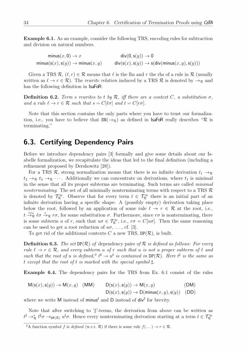
34 Chapter 6. Certification of Termination Proofs using CeTA
Example 6.1. As an example, consider the following TRS, encoding rules for subtractionand division on natural numbers.
minus(x, 0)→ x div(0, s(y))→ 0
minus(s(x), s(y))→ minus(x, y) div(s(x), s(y))→ s(div(minus(x, y), s(y)))
Given a TRS R, (`, r) ∈ R means that ` is the lhs and r the rhs of a rule in R (usuallywritten as `→ r ∈ R). The rewrite relation induced by a TRS R is denoted by →R andhas the following definition in IsaFoR:
Definition 6.2. Term s rewrites to t by R, iff there are a context C, a substitution σ,and a rule `→ r ∈ R such that s = C[`σ] and t = C[rσ].
Note that this section contains the only parts where you have to trust our formaliza-tion, i.e., you have to believe that SN(→R) as defined in IsaFoR really describes “R isterminating.”
6.3. Certifying Dependency Pairs
Before we introduce dependency pairs [3] formally and give some details about our Is-abelle formalization, we recapitulate the ideas that led to the final definition (including arefinement proposed by Dershowitz [28]).
For a TRS R, strong normalization means that there is no infinite derivation t1 →Rt2 →R t3 →R · · · . Additionally we can concentrate on derivations, where t1 is minimalin the sense that all its proper subterms are terminating. Such terms are called minimalnonterminating. The set of all minimally nonterminating terms with respect to a TRS Ris denoted by T ∞R . Observe that for every term t ∈ T ∞R there is an initial part of aninfinite derivation having a specific shape: A (possibly empty) derivation taking placebelow the root, followed by an application of some rule ` → r ∈ R at the root, i.e.,
t>ε∗→R `σ
ε→R rσ, for some substitution σ. Furthermore, since rσ is nonterminating, thereis some subterm u of r, such that uσ ∈ T ∞R , i.e., rσ = C[uσ]. Then the same reasoningcan be used to get a root reduction of uσ, . . . , cf. [3].
To get rid of the additional contexts C a new TRS, DP(R), is built.
Definition 6.3. The set DP(R) of dependency pairs of R is defined as follows: For everyrule ` → r ∈ R, and every subterm u of r such that u is not a proper subterm of ` andsuch that the root of u is defined,2 `] → u] is contained in DP(R). Here t] is the same ast except that the root of t is marked with the special symbol ].
Example 6.4. The dependency pairs for the TRS from Ex. 6.1 consist of the rules
M(s(x), s(y))→ M(x, y) (MM) D(s(x), s(y))→ M(x, y) (DM)
D(s(x), s(y))→ D(minus(x, y), s(y)) (DD)
where we write M instead of minus] and D instead of div] for brevity.
Note that after switching to ’]’-terms, the derivation from above can be written ast] →∗R `]σ →DP(R) u
]σ. Hence every nonterminating derivation starting at a term t ∈ T ∞R2A function symbol f is defined (w.r.t. R) if there is some rule f(. . . )→ r ∈ R.

6.3. Certifying Dependency Pairs 35
can be transformed into an infinite derivation of the following shape where all→DP(R)-stepsare applied at the root.
t] →∗R s]1 →DP(R) t
]1 →∗R s
]2 →DP(R) t
]2 →∗R · · · (1)
Therefore, to prove termination of R it suffices to prove that there is no such derivation.To formalize DPs in Isabelle we modify the signature such that every function symbolnow appears in a plain version and in a ]-version.
datatype ’f shp = Sharp ’f ("_]") | Plain ’f ("_@")
Sharping a term is done via
fun plain :: "(’f,’v)term => (’f shp,’v)term"
where "plain(Var x) = Var x"
| "plain(Fun f ss) = Fun f@ (map plain ss)"
fun sharp :: "(’f,’v)term => (’f shp,’v)term"
where "sharp(Var x) = Var x"
| "sharp(Fun f ss) = Fun f] (map plain ss)"
Thus t] in Def. 6.3 is the same as sharp(t). Since the function symbols in DP(R) areof type ’f shp and the function symbols of R are of type ’f, it is not possible to usethe same TRS R in combination with DP(R). Thus, in our formalization we use thelifting ID—that just applies plain to all lhss and rhss in R.
Considering this technicalities and omitting the initial derivation t] →∗R s]1 from thederivation (1), we obtain
s]1 →DP(R) t]1 →∗ID(R) s
]2 →DP(R) t
]2 →∗ID(R) · · ·
and hence a so called infinite (DP(R), ID(R))-chain. Then the corresponding DP problem(DP(R), ID(R)) is called to be not finite, cf. [40]. Notice that in IsaFoR a DP problem isjust a pair of two TRSs over arbitrary signatures—similar to [40].
In IsaFoR an infinite chain3 and finite DP problems are defined as follows.
fun ichain where "ichain(P ,R) ~s ~t ~σ = (∀i.(~s i,~t i) ∈ P ∧ (~t i)·(~σ i) →∗R (~s(i+1))·(~σ(i+1))"
fun finite_dpp where
"finite_dpp(P ,R) = (¬(∃~s ~t ~σ. ichain (P ,R) ~s ~t ~σ))"
where ‘t · σ’ denotes the application of substitution σ to term t.We formally established the connection between strong normalization and finiteness of
the initial DP problem (DP(R), ID(R)). Although this is a well-known theorem, formal-izing it in Isabelle was a major effort.
Theorem 6.5. wf_trs(R) ∧ finite_dpp(DP(R), ID(R)) −→ SN(→R).
The additional premise wf_trs(R) ensures two well-formedness properties forR, name-ly that for every `→ r ∈ R, ` is not a variable and that Var(r) ⊆ Var(`).
At this point we can obviously switch from the problem of proving SN(→R) for someTRS R, to the problem of proving finite_dpp(DP(R), ID(R)), and thus enter the realm
3We also formalized minimal chains, but here only present chains for simplicity.

36 Chapter 6. Certification of Termination Proofs using CeTA
of the DP framework [40]. Here, the current technique is to apply so-called processors toa DP problem, in order to get a set of simpler DP problems. This is done recursively,until the leafs of the so built tree consist of DP problems with empty P-components (andtherefore are trivially finite). For this to be correct, the applied processors need to besound, i.e., every processor Proc has to satisfy the implication
(∀p ∈ Proc(P ,R). finite_dpp(p)) −→ finite_dpp(P ,R)
for every input. The termination techniques that will be introduced in the followingsections are all such (sound) processors.
So much to the underlying formalization. Now we will present how the check in IsaFoRcertifies a set of DPs P that was generated by some termination tool for some TRS R.To this end, the function checkDPs is used.
checkDPs(P,R) = checkWfTRS(R) ∧ computeDPs(R) ⊆ PHere checkWfTRS checks the two well-formedness properties mentioned above (the
difference between wf_trs and checkWfTRS is that only the latter is executable) andcomputeDPs uses Def. 6.3, which is currently the strongest definition of DPs. To have arobust system, the check does not require that exactly the set of DPs w.r.t. to Def. 6.3 isprovided, but any superset is accepted. Hence we are also able to accept proofs from ter-mination tools that use a weaker definition of DP(R). The soundness result of checkDPsis formulated as follows in IsaFoR.
Theorem 6.6. If checkDPs(P ,R) is accepted, then finiteness of (P , ID(R)) impliesSN(→R).
6.4. Certifying the Dependency Graph Processor
One important processor to prove finiteness of a DP problem is based on the dependencygraph [3, 40]. The dependency graph of a DP problem (P ,R) is a directed graph G =(P , E) where (s → t, u → v) ∈ E iff s → t, u → v is a (P ,R)-chain. Hence, everyinfinite (P ,R)-chain corresponds to an infinite path in G and thus, must end in somestrongly connected component (SCC) S of G, provided that P contains only finitely manyDPs. Dropping the initial DPs of the chain results in an infinite (S,R)-chain.4 Hence,if for all SCCs S of G the DP problem (S,R) is finite, then (P ,R) is finite. In practice,this processor allows to prove termination of each block of mutual recursive functionsseparately.
To certify an application of the dependency graph processor there are two main chal-lenges. First of all, we have to certify that a valid SCC decomposition of G is used, apurely graph-theoretical problem. Second, we have to generate the edges of G. Since thedependency graph G is in general not computable, usually estimated graphs G ′ are usedwhich contain all edges of the real dependency graph G. Hence, for the second problemwe have to implement and certify one estimation of the dependency graph.
Notice that there are various estimations around and that the result of an SCC decom-position depends on the estimation that is used. Hence, it is not a good idea to implementthe strongest estimation and then match the result of our decomposition against somegiven decomposition: problems arise if the termination prover used a weaker estimationand thus obtained larger SCCs.
4We identify an SCC S with the set of nodes S within that SCC.

6.4. Certifying the Dependency Graph Processor 37
Therefore, in the upcoming Sect. 6.4.1 about graph algorithms we just speak of de-compositions where the components do not have to be SCCs. Moreover, we will alsoelaborate on how to minimize the number of tests (s→ t, u→ v) ∈ E. The reason is thatin Sect. 6.4.2 we implemented one of the strongest dependency graph estimations wherethe test for an edge can become expensive. In Sect. 6.4.3 we finally show how to combinethe results of Sections 6.4.1 and 6.4.2.
6.4.1. Certifying Graph Decompositions
Instead of doing an SCC decomposition of a graph within IsaFoR we base our check onthe decomposition that is provided by the termination prover. Essentially, we demandthat the set of components is given as a list 〈C1, . . . , Ck〉 in topological order where thecomponent with no incoming edges is listed first. Then we aim at certifying that everyinfinite path must end in some Ci. Note that the general idea of taking the topologicalsorted list as input was already publicly mentioned at the “Workshop on the certificationof termination proofs” in 2007. In the following we present how we filled the details ofthis general idea.
The main idea is to ensure that all edges (p, q) ∈ E correspond to a step forward in thelist 〈C1, . . . , Ck〉, i.e., (p, q) ∈ Ci × Cj where i ≤ j. However, iterating over all edges ofG will be costly, because it requires to perform the test (p, q) ∈ E for all possible edges(p, q) ∈ P × P . To overcome this problem we do not iterate over the edges but over P .To be more precise, we check that
∀(p, q) ∈ P × P . (∃i ≤ j. (p, q) ∈ Pi × Pj) ∨ (p, q) /∈ E (2)
where the latter part of the disjunction is computed only on demand. Thus, only thoseedges have to be computed, which would contradict a valid decomposition.
Example 6.7. Consider the set of nodes P = {(DD), (DM), (MM)}. Suppose that we haveto check a decomposition of P into L = 〈{(DD)}, {(DM)}, {(MM)}〉 for some graph G =(P , E). Then our check has to ensure that the dashed edges in the following illustrationdo not belong to E.
(DD) (DM) (MM)
It is easy to see that (2) is satisfied for every list of SCCs that is given in topologicalorder. What is even more important, whenever there is a valid SCC decomposition of G,then (2) is also satisfied for every subgraph. Hence, regardless of the dependency graphestimation a termination prover might have used, we accept it, as long as our estimationdelivers less edges.
However, the criterion is still too relaxed, since we might cheat in the input by listingnodes twice. Consider P = {p1, . . . , pm} where the corresponding graph is arbitraryand L = 〈{p1}, . . . , {pm}, {p1}, . . . , {pm}〉. Then trivially (2) is satisfied, because we canalways take the source of edge (pi, pj) from the first part of L and the target from thesecond part of L. To prevent this kind of problem, our criterion demands that the setsCi in L are pairwise disjoint.
Before we formally state our theorem, there is one last step to consider, namely thehandling of singleton nodes which do not form an SCC on their own. Since we cannoteasily infer at what position these nodes have to be inserted in the topological sorted

38 Chapter 6. Certification of Termination Proofs using CeTA
list—this would amount to do an SCC decomposition on our own—we demand that theyare contained in the list of components.5
To distinguish a singleton node without an edge to itself from a “real SCC”, we requirethat the latter ones are marked. Then condition (2) is extended in a way that unmarkedcomponents may have no edge to themselves. The advantage of not marking a componentis that our IsaFoR-theorem about graph decomposition states that every infinite path willend in some marked component, i.e., here the unmarked components can be ignored.
Theorem 6.8. Let L = 〈C1, . . . , Ck〉 be a list of sets of nodes, some of them marked, letG = (P , E) be a graph, let α be an infinite path of G. If
• ∀(p, q) ∈ P × P . (∃i < j. (p, q) ∈ Ci × Cj) ∨ (∃i. (p, q) ∈ Ci × Ci ∧ Ci is marked) ∨(p, q) /∈ E and
• ∀i 6= j. Ci ∩ Cj = ∅
then there is some suffix β of α and some marked Ci such that all nodes of β belong toCi.
Example 6.9. If we continue with example Ex. 6.7 where only components {(MM)} and{(DD)} are marked, then our check also analyzes that G contains no edge from (DM) toitself. If it succeeds, every infinite path will in the end only contain nodes from {(DD)}or only nodes from {(MM)}. In this way, only 4 edges of G have to be calculated insteadof analyzing all 9 possible edges in P × P .
6.4.2. Certifying Dependency Graph Estimations
What is currently missing to certify an application of the dependency graph processor,is to check, whether a singleton edge is in the dependency graph or not. Hence, wehave to estimate whether the sequence s → t, u → v is a chain, i.e., whether there aresubstitutions σ and µ such that tσ →∗R uµ. An obvious solution is to just look at theroot symbols of t and u—if they are different there is no way that the above condition ismet (since all the steps in tσ →∗R uµ take place below the root, by construction of thedependency pairs). Although efficient and often good enough, there are more advancedestimations around.
The estimation EDG [3] first replaces via an operation cap all variables and all subtermsof t which have a defined root-symbol by distinct fresh variables. Then if cap(t) and u donot unify, it is guaranteed that there is no edge.
The estimation EDG∗[50] does the same check and additionally uses the reversed TRSR−1 = {r → ` | `→ r ∈ R}, i.e., it uses the fact that tσ →∗R uµ implies uµ→∗R−1 tσ andchecks whether cap(u) does not unify with t. Of course in the application of cap(u) wehave to take the reversed rules into account (possibly changing the set of defined symbols)and it is not applicable if R contains a collapsing rule `→ x where x ∈ V .
The last estimation we consider is based on a better version of cap, called tcap [41]. Itonly replaces subterms with defined symbols by a fresh variable, if there is a rule thatunifies with the corresponding subterm.
Definition 6.10. Let R be a TRS.
5Note that Tarjan’s SCC decomposition algorithm produces exactly this list.

6.4. Certifying the Dependency Graph Processor 39
• tcap(f(~tn)) = f(tcap(t1), . . . , tcap(tn)) iff f(tcap(t1), . . . , tcap(tn)) does not unifywith any variable renamed left-hand side of a rule from R
• tcap(t) is a fresh variable, otherwise
To illustrate the difference between cap and tcap consider the TRS of Ex. 6.1 andt = div(0, 0). Then cap(t) = xfresh since div is a defined symbol. However, tcap(t) = tsince there is no division rule where the second argument is 0.
Apart from tree automata techniques, currently the most powerful estimation is theone based on tcap looking both forward as in EDG and backward as in EDG∗. Hence, weaimed to implement and certify this estimation in IsaFoR.
Unfortunately, when doing so, we had a problem with the domain of variables. Theproblem was that although we first implemented and certified the standard unificationalgorithm of [78], we could not directly apply it to compute tcap. The reason is that togenerate fresh variables as well as to rename variables in rules apart, we need a type ofvariables with an infinite domain. One solution would have been to constrain the type ofvariables where there is a function which delivers a fresh variable w.r.t. any given finiteset of variables.
However, there is another and more efficient approach to deal with this problem thanthe standard approach to rename and then do unification. Our solution is to switch toanother kind of terms where instead of variables there is just one special constructor“2” representing an arbitrary fresh variable. In essence, this data structure representscontexts which do not contain variables, but where multiple holes are allowed. Thereforein the following we speak of ground-contexts and use C,D, . . . to denote them.
Definition 6.11. Let JCK be the equivalence class of a ground-context C where the holesare filled with arbitrary terms: JCK = {C[t1, . . . , tn] | t1, . . . , tn ∈ T (F ,V)}.
Obviously, every ground-context C can be turned into a term t which only containsdistinct fresh variables and vice-versa. Moreover, every unification problem between tand ` can be formulated as a ground-context matching problem between C and `, whichis satisfiable iff there is some µ such that `µ ∈ JCK.
Since the result of tcap is always a term which only contains distinct fresh variables,we can do the computation of tcap using the data structure of ground-contexts; it onlyrequires an algorithm for ground-context matching. To this end we first generalize ground-context matching problems to multiple pairs (Ci, `i).
Definition 6.12. A ground-context matching problem is a set of pairs M = {(C1, `1),. . . , (Cn, `n)}. It is solvable iff there is some µ such that `iµ ∈ JCiK for all 1 ≤ i ≤ n. Wesometimes abbreviate {(C, `)} by (C, `).
To decide ground-context matching we devised a specialized algorithm which is similarto standard unification algorithms, but which has some advantages: it does neither requireoccur-checks as the unification algorithm, nor is it necessary to preprocess the left-handsides of rules by renaming (as would be necessary for standard tcap). And instead ofapplying substitutions on variables, we just need a basic operation on ground-contextscalled merge such that merge(C,D) = ⊥ implies JCK ∩ JDK = ∅, and merge(C,D) = Eimplies JCK ∩ JDK = JEK.

40 Chapter 6. Certification of Termination Proofs using CeTA
Definition 6.13. The following rules simplify a ground-context matching problem intosolved form (where all terms are distinct variables) or into ⊥.
(a) M∪ {(2, `)} ⇒match M(b) M∪ {(f(~Dn), f(~un))} ⇒match M∪ {(D1, u1), . . . , (Dn, un)}(c) M∪ {(f(~Dn), g(~uk))} ⇒match ⊥ if f 6= g or n 6= k(d) M∪ {(C, x), (D, x)} ⇒match M∪ {(E, x)} if merge(C,D) = E(e) M∪ {(C, x), (D, x)} ⇒match ⊥ if merge(C,D) = ⊥
Rules (a–c) obviously preserve solvability of M (where ⊥ represents an unsolvablematching problem). For Rules (d,e) we argue as follows:
{(C, x), (D, x)} ∪ . . . is solvable iff
• there is some µ such that xµ ∈ JCK and xµ ∈ JDK and . . . iff
• there is some µ such that xµ ∈ JCK ∩ JDK and . . . iff
• there is some µ such that xµ ∈ Jmerge(C,D)K and . . . iff
• {(merge(C,D), x)} ∪ . . . is solvable
Since every ground-context matching problem in solved form is solvable, we have deviseda decision procedure. It can be implemented in two stages where the first stage justnormalizes by the Rules (a–c), and the second stage just applies the Rules (d,e). Itremains to implement merge.
merge(2, C)⇒merge C
merge(C,2)⇒merge C
merge(f(~Cn), g(~Dk))⇒merge ⊥ if f 6= g or n 6= k
merge(f(~Cn), f(~Dn))⇒merge f(merge(C1, D1), . . . ,merge(Cn, Dn))
f(. . . ,⊥, . . .)⇒merge ⊥
Note that our implementations of the matching algorithm and the merge function inIsaFoR are slightly different due to different data structures. For example matching prob-lems are represented as lists of pairs, so it may occur that we have duplicates inM. Thedetails of our implementation can be seen in IsaFoR (theory Edg) or in the source of CeTA.
Soundness and completeness of our algorithms are proven in IsaFoR.
Theorem 6.14. • If merge(C,D)⇒∗merge ⊥ then JCK ∩ JDK = ∅.
• If merge(C,D)⇒∗merge E then JCK ∩ JDK = JEK.
• If (C, `)⇒∗match ⊥ then there is no µ such that `µ ∈ JCK.
• If (C, `) ⇒∗match M where M is in solved form, then there exists some µ such that`µ ∈ JCK.
Using ⇒match, we can now easily reformulate tcap in terms of ground-context matchingwhich results in the efficient implementation etcap.
Definition 6.15. • etcap(f(~tn)) = f(etcap(t1), . . . , etcap(tn)) iff(f(etcap(t1), . . . , etcap(tn)), `)⇒∗match ⊥ for all rules `→ r ∈ R.

6.5. Certifying the Reduction Pair Processor 41
• 2, otherwise
One can also reformulate the desired check to estimate the dependency graph whethertcap(t) does not unify with u in terms of etcap. It is the same requirement as demanding(etcap(t), u)⇒∗match ⊥. Again, the soundness of this estimation has been proven in IsaFoRwhere the second part of the theorem is a direct consequence of the first part by usingthe soundness of the matching algorithm.
Theorem 6.16. (a) Whenever tσ →∗R s then s ∈ Jetcap(t)K.
(b) Whenever tσ →∗R uτ then (etcap(t), u) 6⇒∗match ⊥ and (etcap(u), t) 6⇒∗match ⊥ whereetcap(u) is computed w.r.t. the reversed TRS R−1.
6.4.3. Certifying Dependency Graph Decomposition
Eventually we can connect the results of the previous two subsections to obtain onefunction to check a valid application of the dependency graph processor.
checkDepGraphProc(P , L,R) = checkDecomposition(checkEdg(R),P , L)
where checkEdg just applies the criterion of Thm. 6.16 (b).In IsaFoR the soundness result of our check is proven.
Theorem 6.17. If checkDepGraphProc(P , L,R) is accepted and if for all P ′ ∈ L whereP ′ is marked, the DP problem (P ′,R) is finite, then (P ,R) is finite.
To summarize, we have implemented and certified the currently best dependency graphestimation which does not use tree automata techniques. Our check-function accepts anydecomposition which is based on a weaker estimation, but requires that the componentsare given in topological order. Since our algorithm computes edges only on demand, thenumber of tests for an edge is reduced considerably. For example, the five largest graphsin our experiments contain 73,100 potential edges, but our algorithm only has to consider31,266. This reduced the number of matchings from 13 millions down to 4 millions.
Furthermore, our problem of not being able to generate fresh variables or to renamevariables in rules apart led to a more efficient algorithm for tcap based on matching insteadof unification: simply replacing tcap by etcap in TTT2 reduced the time for estimating thedependency graph by a factor of two.
6.5. Certifying the Reduction Pair Processor
One important technique to prove finiteness of a DP problem (P ,R) is the so-calledreduction pair processor. The general idea is to use a well-founded order where all rulesof P ∪ R are weakly decreasing. Then we can delete all strictly decreasing rules from Pand continue with the remaining dependency pairs.
We first state a simplified version of the reduction pair processor as it is introduced in[40], where we ignore the usable rules refinement.
Theorem 6.18. If all the following properties are satisfied, then finiteness of (P \�,R)implies finiteness of (P ,R).
(a) � is a well-founded and stable order

42 Chapter 6. Certification of Termination Proofs using CeTA
(b) % is a stable and monotone quasi-order
(c) % ◦ � ⊆ � and � ◦% ⊆ �
(d) P ⊆ � ∪% and R ⊆ %
Of course, to instantiate the reduction pair processor with a new kind of reduction pair,e.g., LPO, polynomial orders,. . . , we first have to prove the first three properties for thatkind of reduction pairs. Since we plan to integrate many reduction pairs, but only wantto write the reduction pair processor once, we tried to minimize these basic requirementssuch that the reduction pair processor still remains sound in total. In the end, we replacedthe first three properties by:
(a) � is a well-founded and stable relation
(b) % is a stable and monotone relation
(c) % ◦ � ⊆ �
In this way, for every new class of reduction pairs, we do not have to prove transitivityof � or % anymore, as it would be required for Thm. 6.18. Currently, we just supportreduction pairs based on polynomial interpretations with negative constants [51], but weplan to integrate other reduction pairs in the future.
For checking an application of a reduction pair processor we implemented a genericfunction checkRedPairProc in Isabelle, which works as follows. It takes as input twofunctions checkS and checkNS which have to approximate a reduction pair, i.e., whenevercheckS(s, t) is accepted, then s � t must hold in the corresponding reduction pair andsimilarly, checkNS has to guarantee s % t.
Then checkRedPairProc(checkS, checkNS,P ,P ′,R) works as follows:
• iterate once over P to divide P into P� and P6� where the former set contains allpairs of P where checkS is accepted
• ensure for all s→ t ∈ R ∪ P 6� that checkNS(s, t) is accepted, otherwise reject
• accept if P6� ⊆ P ′, otherwise reject
The corresponding theorem in IsaFoR states that a successful application of checkRed-PairProc(. . . ,P ,P ′,R) proves that (P ,R) is finite whenever (P ′,R) is finite. Obviously,the first two conditions of checkRedPairProc ensure condition (d) of Thm. 6.18. Note,that it is not required that all strictly decreasing pairs are removed, i.e., our checks maybe stronger than the ones that have been used in the termination provers.
6.6. Certifying the Whole Proof Tree
From Sect. 6.3–6.5 we have basic checks for the three techniques of applying dependencypairs (checkDPs), the dependency graph processor (checkDepGraphProc), and the re-duction pair processor (checkRedPairProc). For representing proof trees within the DPframework we used the following data structures in IsaFoR.

6.6. Certifying the Whole Proof Tree 43
datatype ’f RedPair = NegPolo "(’f × (cint × nat list))list"
datatype (’f,’v)DPProof = . . . 6
| PisEmpty
| RedPairProc "’f RedPair" "(’f,’v)trsL" "(’f,’v)DPProof"
| DepGraphProc "((’f,’v)DPProof option × (’f,’v)trsL)list"
datatype (’f,’v)TRSProof = . . . 6
| DPTrans "(’f shp,’v)trsL" "(’f shp,’v)DPProof"
The first line fixes the format for reduction pairs, i.e., currently of (linear) polynomialinterpretations where for every symbol there is one corresponding entry. E.g., the list[(f, (−2, [0, 3]))] represents the interpretation where Pol(f)(x, y) = max(−2 + 3y, 0) andPol(g)(x1, . . . , xn) = 1 + Σ1≤i≤nxi for all f 6= g.
The datatype DPProof represents proof trees for DP problems. Then the check for validDPProofs gets as input a DP problem (P ,R) and a proof tree and tries to certify that(P ,R) is finite. The most basic technique is the one called PisEmpty, which demandsthat the set P is empty. Then (P ,R) is trivially finite.
For an application of the reduction pair processor, three inputs are required. First, thereduction pair redp, i.e., some polynomial interpretation. Second, the dependency pairsP ′ that remain after the application of the reduction pair processor. Here, the datatypetrsL is an abbreviation for lists of rules. And third, a proof that the remaining DP prob-lem (P ′,R) is finite. Then the checker just has to call createRedPairProc(redp,P ,P ′,R)and additionally calls itself recursively on (P ′,R). Here, createRedPairProc invokescheckRedPairProc where checkS and checkNS are generated from redp.
The most complex structure is the one for decomposition of the (estimated) dependencygraph. Here, the topological list for the decomposition has to be provided. Moreover, foreach subproblem P ′, there is an optional proof tree. Subproblems where a proof is givenare interpreted as “real SCCs” whereas the ones without proof remain unmarked for thefunction checkDepGraphProc.
The overall function for checking proof trees for DP problems looks as follows.
checkDPProof(P,R,PisEmpty) = (P = [])
checkDPProof(P,R,(RedPairProc redp P ′ prf)) =
createRedPairProc(redp,P,P ′,R) ∧ checkDP(P ′,R,prf)checkDPProof(P,R,DepGraphProc P ′s) =
checkDepGraphProc(P,map (λ(prfO,P ′).(isSome prfO,P ′)) P ′s, R)∧
∧(Some prf,P ′)∈P ′s checkDPProof(P ′,R,prf)
Theorem 6.19. If checkDPProof(P,R,prf) is accepted then (P ,R) is finite.
Using checkDPProof it is now easy to write the final method checkTRSProof for provingtermination of a TRS, where computeID is an implementation of ID.
checkTRSProof(R,DPTrans P prf) =
checkDPs(R,P) ∧ checkDPProof(P,computeID(R),prf)For the external usage of CeTA we developed a well documented XML-format, cf. CeTA’s
website. Moreover, we implemented two XML parsers in Isabelle, one that transforms agiven TRS into the internal format, and another that does the same for a given proof.
6CeTA supports even more techniques, cf. CeTA’s website for a complete list.

44 Chapter 6. Certification of Termination Proofs using CeTA
The function certifyProof, finally, puts everything together. As input it takes twostrings (a TRS and its proof). Then it applies the mentioned parsers and afterwards callscheckTRSProof on the result.
Theorem 6.20. If certifyProof(R,prf) is accepted then SN(→R).
To ensure that the parser produces the right TRS, after the parsing process it is checkedthat when converting the internal data-structures of the TRS back to XML, we get thesame string as the input string for the TRS (modulo whitespace). This is a major benefitin comparison to the two other approaches where it can and already has happened thatthe uncertified components Rainbow/CiME produced a wrong proof goal from the inputTRS, i.e., they created a termination proof within Coq for a different TRS than the inputTRS.
6.7. Error Messages
To generate readable error messages, our checks do not have a Boolean return type,but a monadic one (isomorphic to ’e option). Here, None represents an accepted checkwhereas Some e represents a rejected check with error message e. The theory ErrorMonad
contains several basic operations like >> for conjunction of checks, <- for changing theerror message, and isOK for testing acceptance.
Using the error monad enables an easy integration of readable error messages. Forexample, the real implementation of checkTRSProof looks as follows:
fun checkTRSProof where "checkTRSProof R (DPTrans P prf) = (
checkDPs R P
<- (λs. ’’error . . .’’ @ showTRS R @ ’’. . .’’ @ showTRS P @ s)
>> checkDPProof P (computeID R) prf
<- (λs. ’’error below switch to dependency pairs’’ @ s))"
However, since we do not want to adapt the proofs every time the error messages arechanged, we setup the Isabelle simplifier such that it hides the details of the error monad,but directly removes all the error handling and turns monadic checks via isOK(...) intoBoolean ones using the following lemmas.
lemma "isOK(m >> n) = isOK(m) ∧ isOK(n)"
lemma "isOK(m <- s) = isOK(m)"
Then, for example, isOK(checkTRSProof R (DPTrans P prf)) directly simplifies toisOK(checkDPs R P) ∧ isOK(checkDPProof P (computeID R) prf).
6.8. Experiments and Conclusion
Isabelle’s code-generator is invoked to create CeTA from IsaFoR. To compile CeTA one aux-iliary hand-written Haskell file CeTA.hs is needed, which just reads two files (one for theTRS, one for the proof) and then invokes certifyProof.
We tested CeTA (version 1.03) using TTT2 as termination prover (TC and TC+). Here,TTT2 uses only the techniques of this paper in the combination TC, whereas in TC+ allsupported techniques are tried, including usable rules and nontermination. We compareto CiME/Coccinelle using AProVE [39] or CiME [22] as provers (ACC,CCC), and to Rain-bow/CoLoR using AProVE or Matchbox [106] (ARC,MRC) where we take the results of

6.8. Experiments and Conclusion 45
the latest certified termination competition in Nov 20087 involving 1391 TRSs from thetermination problem database.
We performed our experiments using a PC with a 2.0 GHz processor running Linuxwhere both TTT2 and CeTA where aborted after 60 seconds. The following table summarizesour experiments and the termination competition results.
TC TC+ ACC CCC ARC MRCproved / disproved 401 / 0 572 / 214 532 / 0 531 / 0 580 / 0 458 / 0
certified 391 / 0 572 / 214 437 / 0 485 / 0 558 / 0 456 / 0rejected 10 0 3 0 0 2
cert. timeouts 0 0 92 46 22 0total cert. time 33s 113s 6212s 6139s 7004s 3602s
The 10 proofs that CeTA rejected are all for nonterminating TRSs which do not satisfythe variable condition. Since TC supports only polynomial orders as reduction pairs, itcan handle less TRSs than the other combinations. But, there are 44 TRSs which areonly solved by TC (and TC+), the reason being the time-limit of 60 seconds (19 TRSs),the dependency graph estimation (8 TRSs), and the polynomial order allowing negativeconstants (17 TRSs).
The second line clearly shows that TC+ (with nontermination and usable rules support)currently is the most powerful combination with 786 certified proofs. Moreover, TC+ canhandle 214 nonterminating and 102 terminating TRSs where none of ACC, CCC, ARC,and MRC were successful. The efficiency of CeTA is also clearly visible: the averagecertification time in TC and TC+ for a single proof is by a factor of 50 faster than in theother combinations.8
For more details on the experiments we refer to CeTA’s website.To conclude, we presented a modular and competitive termination certifier, CeTA, which
is directly created from our Isabelle library on term rewriting, IsaFoR. Its main featuresare that CeTA is available as a stand-alone binary, the efficiency, the dependency graphestimation, nontermination and usable rules support, the error handling, and the robust-ness.
As each sub-check for a termination technique can be called separately, and as our checkto certify a whole termination proof just invokes these sub-checks, it seems possible tointegrate other techniques (even if they are proved in a different theorem prover) as longas they are available as executable code. However, we will need a common proof formatand a compatible definition.
As future work we plan to certify several other termination techniques where we alreadymade progress in the formalization of semantic labeling and the subterm-criterion. Wewould further like to contribute to a common proof format.
7http://termcomp.uibk.ac.at/8Note that in the experiments above, for each TRS, each combination might have certified a different
proof. In an experiment where the certifiers where run on the same proofs for each TRS (using onlytechniques that are supported by all certifiers, i.e., EDG and linear polynomials without negativeconstants), CeTA was even 190 times faster than the other approaches and could certify all 358 proofs,whereas each of the other two approaches failed on more than 30 proofs due to timeouts.


7. Certified Subterm Criterion andCertified Usable Rules
Publication details
Christian Sternagel and Rene Thiemann. Certified Subterm Criterion and Certified Us-able Rules. In Proceedings of the 21st International Conference on Rewriting Techniquesand Applications, volume 6 of LIPIcs, pages 325–340. Schloss Dagstuhl – Leibniz-Zentrumfur Informatik, 2010.
Abstract
In this paper we present our formalization of two important termination techniques forterm rewrite systems: the subterm criterion and the reduction pair processor in combi-nation with usable rules. For both techniques we developed executable check functionsusing the theorem prover Isabelle/HOL. These functions are able to certify the correctapplication of the formalized techniques in a given termination proof. As there are severalvariants of usable rules, we designed our check function in such a way that it accepts allknown variants, even those which are not explicitly spelled out in previous papers.
We integrated our formalization in the publicly available IsaFoR-library. This led toa significant increase in the power of CeTA, a certified termination proof checker that isextracted from IsaFoR.
7.1. Introduction
Termination provers for term rewrite systems (TRSs) became more and more powerful inthe last years. One reason is that a proof of termination no longer is just some reductionorder which contains the rewrite relation of the TRS. Currently, most provers constructa proof in the dependency pair framework (DP framework). This allows to combine basictermination techniques in a flexible way. Hence, a termination proof is a tree where ateach node a specific technique is applied. So instead of just stating the precedence of somelexicographic path order or giving some polynomial interpretation, current terminationprovers return proof trees consisting of many different techniques and reaching sizes ofseveral megabytes. Thus, it would be too much work to check by hand whether thesetrees really form a valid proof. (Additionally, checking by hand does not provide a veryhigh degree of confidence.)
It is regularly demonstrated that we cannot blindly trust in the output of terminationprovers. Every now and then, some termination prover delivers a faulty proof. Mostoften, this is only detected if there is another prover giving a contradicting answer on thesame problem. To solve this problem, three systems have been developed over the lastfew years: CiME/Coccinelle [21, 23], Rainbow/CoLoR [12], and CeTA/IsaFoR [104]. Thesesystems either certify or reject a given termination proof. Here, Coccinelle and CoLoR

48 Chapter 7. Certified Subterm Criterion and Certified Usable Rules
are libraries on rewriting for Coq (http://coq.inria.fr) and IsaFoR is our library onrewriting for Isabelle [84]. (Throughout this paper we just write Isabelle whenever werefer to Isabelle/HOL.)
All of these certifiers can automatically certify termination proofs that are performedwithin the DP framework. In this framework one tries to simplify so called DP problems(P ,R) by processors until all pairs in P are removed.
The reduction pair processor [42, 50] is the major technique to remove pairs. Conse-quently, it has been formalized in all three libraries. One of the conditions of the processordemands that all rules in R must be weakly decreasing. If this and all other conditionsare satisfied then one can remove all strictly decreasing pairs. In this paper, we presentthe details about the formalization of two important extensions of the reduction pairprocessor.
The first extension is the subterm criterion [51]. By restricting the used “reduction pair”to the subterm relation in combination with simple projections, it is possible to ignorethe R-component of a DP problem. Note that the subterm criterion has independently(and only recently) been formalized for the Coccinelle-library [23]. Here, we present thefirst Isabelle formalization of this important technique.
The other extension is the integration of usable rules [40–42, 50, 105]. With this ex-tension not all rules in R have to be weakly decreasing but only the usable rules whichare most often a strict subset of R. However, there are several definitions of usable ruleswhere the most powerful ones ([41] and [42]) are incomparable.
all rules usable rules ([105]) usable rules ([40,50])usable rules ([42])
usable rules ([41])⊇ ⊇ ⊇⊇
Although it was often stated that a combination of the definitions of usable rules of [41]and [42] would be possible there never was a refereed paper which showed such a proof.(However, there have been unpublished soundness proofs of such a combined definition.)In this paper we not only present such a combined definition and the first correspondingformalized soundness proof, but we also simplified and extended the existing proofs. Forexample, we never construct filtered terms although we consider usable rules w.r.t. someargument filter. (An independent formalization of usable rules is present in Coccinelle.However, this formalization is unpublished and it only uses the variant of [50]: it does notfeature the improvements from [41] and [42].) With these two extensions of the reductionpair processor we could increase the number of TRSs (from the Termination ProblemDatabase) where a proof can be certified by our certifier CeTA by over 50%.
Note that all the proofs that are presented (or omitted) in the following, have beenformalized in our Isabelle library IsaFoR. Hence, in the paper we merely give sketches ofour “real” proofs. Our goal is to show the general proof outlines and help to understandthe full proofs. Our library IsaFoR with all formalized proofs, the executable certifier CeTA,and all details about our experiments are available at CeTA’s website:
http://cl-informatik.uibk.ac.at/software/ceta
The paper is structured as follows: In Sec. 7.2, we recapitulate the required notionsand notations of term rewriting and the DP framework. In Sec. 7.3, we describe ourformalization of the subterm criterion. The reduction pair processor with usable rulesand its formalization is presented in Sec. 7.4. Then, in Sec. 7.5, we shortly describe howCeTA is obtained from IsaFoR and give a summary about our experiments. We finallyconclude in Sec. 7.6.

7.2. Preliminaries 49
7.2. Preliminaries
Term Rewriting. We assume familiarity with term rewriting [5]. Still, we recall themost important notions that are used later on. A (first-order) term t over a set ofvariables V and a set of function symbols F is either a variable x ∈ V or an n-ary functionsymbol f ∈ F applied to n argument terms f(~tn). A context C is a term containing exactlyone occurrence of the special constant 2 (that is assumed to be distinct from symbols inF). Replacing 2 in a context C by a term t is denoted by C[t]. A term t is a (proper)subterm of a term s—written (s B t) s D t—whenever there exists a context C ( 6= 2),such that s = C[t]. We write s ≈ t iff s and t are unifiable. An argument filter π is amapping from symbols to integers or lists of integers. It induces a mapping from terms toterms where π(x) = x, π(f(~tn)) = π(ti) if π(f) = i, and π(f(~tn)) = f(π(ti1), . . . , π(tik))if π(f) = [i1, . . . , ik]. Argument filters are also used to indicate which positions in a termare regarded. Then π maps symbols to sets of positions. It will be clear from the contextwhich kind of argument filters is used.
A rewrite rule is a pair of terms ` → r and a TRS R is a set of rewrite rules. Therewrite relation (induced by R) →R is the closure under substitutions and under contextsof R, i.e., s→R t iff there is a context C, a rewrite rule `→ r ∈ R, and a substitution σsuch that s = C[`σ] and t = C[rσ]. Reductions at the root are denoted by →R,ε.
We say that an element t is terminating / strongly normalizing (w.r.t. some binary re-lation S), and write SNS(t), if it cannot start an infinite sequence
t = t1 S t2 S t3 S · · · .
The whole relation is terminating, written SN(S), if all elements are terminating w.r.t. it.For a TRS R and a term t, we write SN(R) and SNR(t) instead of SN(→R) and SN→R(t).We write S+ for the transitive closure of S, and S∗ is the reflexive transitive closure.
Lemma 7.1 (Properties of Subterms).
(a) stability: s B t =⇒ sσ B tσ
(b) subterms preserve termination: SNR(s) ∧ s B t =⇒ SNR(t).
Let →SN(R) denote the restriction of →R to terminating terms, i.e., {(s, t) | s →Rt ∧ SNR(s)}. Let
B→SN(R) denote the same relation extended by the restriction of B toterminating terms, i.e., →SN(R) ∪ {(s, t) | s B t ∧ SNR(s)}.
Lemma 7.2 (Termination Properties). Let S be some binary relation, let R be a TRS.
(a) SN(S)⇐⇒ SN(S+),
(b) SN(B→SN(R)),
(c) SNS(s) ∧ (s, t) ∈ S =⇒ SNS(t).
Dependency Pair Framework. The DP framework [42] is a way to modularize terminationproofs. Therefore, we switch from TRSs to so called DP problems, consisting of two TRSs.The initial DP problem for a TRSR is (DP(R),R) where DP(R) are the dependency pairsof R. A (P ,R)-chain is a possibly infinite derivation of the following form:
s1σ1 →P t1σ1 →∗R s2σ2 →P t2σ2 →∗R s3σ3 →P · · · (?)

50 Chapter 7. Certified Subterm Criterion and Certified Usable Rules
where si → ti ∈ P for all i > 0 (this implies that P-steps only occur at the root). Ifadditionally every tiσi is terminating w.r.t. R, then the chain is minimal. A DP problem(P ,R) is called finite [42], if there is no minimal (P ,R)-chain. Proving finiteness ofa DP problem is done by simplifying (P ,R) by so called processors recursively, untilthe P-components of all remaining DP problems are empty and therefore trivially finite.For this to be correct, the applied processors need to be sound. A processor Proc issound whenever for all DP problems (P ,R) we have that finiteness of (P ′,R′) for all(P ′,R′) ∈ Proc(P ,R) implies finiteness of (P ,R). The termination techniques that willbe introduced in the following sections are all such sound processors.1
Example 7.3. In the following TRS R the term set(xs) evaluates to the list [x ∈ xs |0 < x] where duplicates are removed:
x < 0→ ⊥, (1)
0 < s(y)→ >, (2)
s(x) < s(y)→ x < y, (3)
set(nil)→ nil,
set(x : z)→ if2(0 < x, x, z),
del(x, nil)→ nil, (4)
del(x, y : z)→ if(x < y, y < x, x, y, z), (5)
if(⊥,⊥, x, y, z)→ del(x, z), (6)
if(>, b, x, y, z)→ y : del(x, z), (7)
if(b,>, x, y, z)→ y : del(x, z), (8)
if2(>, x, z)→ x : set(del(x, z)),
if2(⊥, x, z)→ set(z).
After computing the initial DP problem (DP(R),R) we can split it into the threeproblems ({(9)},R), ({(13)–(16)},R), and ({(10)–(12)},R). (This is done by applyingthe dependency graph processor [3,41,42,50], a well-known technique to perform separatetermination proofs for each recursive function.)
s(x) <] s(y)→ x <] y, (9)
set](x : z)→ if2](0 < x, x, z), (10)
if2](>, x, z)→ set](del(x, z)), (11)
if2](⊥, x, z)→ set](z), (12)
del](x, y : z)→ if](x < y, y < x, x, y, z), (13)
if](⊥,⊥, x, y, z)→ del](x, z), (14)
if](>, b, x, y, z)→ del](x, z), (15)
if](b,>, x, y, z)→ del](x, z). (16)
7.3. The Subterm Criterion
The subterm criterion [51] is a termination technique that can be employed as a processorof the DP framework. It may be seen as a variant of the reduction pair processor withan attached argument filtering [3]. The used orders (B and D) allow to ignore the Rcomponent of a DP problem (P ,R). And the argument filtering is restricted to be a socalled simple projection. A simple projection π maps a term to one of its arguments, i.e.,π(f(~tn)) = ti for some 0 < i 6 n. For convenience we use Rπ to denote the ’composition’of the binary relation on terms R and π, i.e., (s, t) ∈ Rπ iff (π(s), π(t)) ∈ R.
Theorem 7.4. Finiteness of (P \Bπ,R) implies finiteness of (P ,R), provided:
(a) all rules of P are oriented by Dπ (i.e., P ⊆ Dπ)
1To be more precise, in IsaFoR it is shown that all these processors are chain identifying (chain identi-
fying proc) which is a slightly stronger requirement than soundness [101, Chapter 7]. The reason isthat chain identifying processors can easily be combined with semantic labeling [110]. However, weomit the details here and just refer to theory DpFramework for the interested reader.

7.3. The Subterm Criterion 51
(b) all lhss and rhss of P are non-variable and non-constant terms where the roots ofrhss are not defined in R (i.e., s = f(~sn) with n > 0 and t = g(~tm) with m > 0 andg /∈ DR for all s→ t ∈ P)
Example 7.5. The DP problem ({(9)},R) from Ex. 7.3 can be solved using the simpleprojection π(<]) = 1, since π(s(x) <] s(y)) = s(x) B x = π(x <] y). Taking π(del]) = 2and π(if]) = 5 we can remove Pair (13) from ({(13)–(16)},R). The result ({(14)–(16)},R)is then solved by the dependency graph processor. Removing a pair from ({(10)–(12)},R)is impossible as there is no π such that Pair (11) is oriented. Note that<], del], if], . . . /∈ DRwhereas <, del, if, · · · ∈ DR.
Before we can prove Theorem 7.4, we need several lemmas. First, we prove that termi-nation of some element w.r.t. some binary relation S is equivalent to termination of thesame element w.r.t. S+. Note that this is a more general result than Lem. 7.2(a) and thusallows termination analysis of a single term, no matter if the whole TRS is terminating.
Lemma 7.6. SNS(t)⇐⇒ SNS+(t).
Proof. The direction from right to left is trivial. For the other direction assume that t isnot terminating w.r.t. S+. Hence t = t1 S
+ t2 S+ t3 S
+ · · · . Let S ′ denote the restrictionof R to terminating terms, i.e., S ′= {(s, t) | s S t ∧ SNS(s)}. By definition we haveSN(S ′) and with Lem. 7.2(a) also SN(S ′+). Using SNS(t) and Lem. 7.2(c) together withthe infinite sequence from above, we get SNS(ti) for all i > 0, and further t1 S
′+ t2 S′+
t3 S′+ · · · . This contradicts SN(S ′+).
Next consider a general result on infinite sequences conducted in the union of two binaryrelations N and S where often N is a non-strict relation and S a strongly normalizingrelation. Intuitively it states the following: Assume that there is an infinite sequence ofsteps, where each step is an N -step or an S-step. Further assume that whenever thereis an N -step directly followed by an S-step, those two steps can be turned into a singleS-step. Additionally, there is no infinite S-sequence starting at the same point as thesequence we are reasoning about. Then, from some point in our sequence on, there areno more S-steps, i.e., it ends in N -steps. This is a versatile fact that is used at severalplaces inside IsaFoR.
Lemma 7.7. Let N and S be two binary relations over some carrier and ~q an infinitesequence of carrier elements. If
(a) (qi, qi+1) ∈ N ∪ S for all i > 0,
(b) N ◦ S ⊆ S, and
(c) SNS(q1),
then there is some j such that for all i ≥ j we have (qi, qi+1) ∈ N \ S.
Proof. For the sake of a contradiction assume that the lemma does not hold. Then,together with (a), we obtain ∀i > 0.∃j ≥ i. (qj, qj+1) ∈ S. Using the Axiom of Choice weget hold of a choice function f such that
∀i > 0. f(i) ≥ i ∧ (qf(i), qf(i)+1) ∈ S, (†)

52 Chapter 7. Certified Subterm Criterion and Certified Usable Rules
i.e., f(i) produces some index of an S-step after position i in ~q. Using f we define a newsequence [·] of indices inductively
[i] =
{i if i = 1,
f([i− 1]) + 1 otherwise.
With (†) we have f(i) ≥ i and (qf(i), qf(i)+1) ∈ S for all i > 0. Since f(i) ≥ i there is anN ∪ S sequence from every qi to the corresponding qf(i). Thus we obtain (qi, qf(i)+1) ∈S+
for all i > 0 using (b). This immediately implies (q[i], q[i+1]) ∈S+ for all i > 0 andthereby ¬SNS+(q[1]) which is equivalent to ¬SNS(q[1]) by Lem. 7.6. But q[1] = q1 and thus¬SNS(q1). Together with (c), this provides the desired contradiction.
Lemma 7.8. SNR(t) =⇒ SN(B∪→R)(t).
Proof. Assume that t is not terminating w.r.t. (B ∪→R). Hence, we obtain the infinitesequence t = t1 (B ∪→R) t2 (B ∪→R) t3 (B ∪→R) · · · . From the assumption we haveSNR(t1) and by Lem. 7.1 and Lem. 7.2(c) we obtain SNR(ti) for all i > 0. Thus, ti
B→SN(R)
ti+1 for all i and since SN(B→SN(R)) by Lem. 7.2(b) we arrive at a contradiction.
Proof of Theorem 7.4. In order to show that finiteness of (P \Bπ,R) implies finiteness of(P ,R) we prove its contraposition. Hence, we may assume (in addition to the premisesof Theorem 7.4) that there is a minimal infinite (P ,R)-chain and have to transform itinto a minimal infinite (P \Bπ,R)-chain. Thus we may assume that for all i > 0:
(a) si → ti ∈ P ,
(b) tiσi →∗R si+1σi+1, and
(c) SNR(tiσi).
We start by a case distinction on ∃j > 0.∀i ≥ j. (si, ti) ∈ (P \Bπ). If there is such a j, wecan combine this with (b) and obtain the desired minimal (P \ Bπ,R)-chain by shiftingthe original chain j positions to the left. Hence, consider the second case and assume∀i > 0. ∃j ≥ i. (sj, tj) /∈ (P \Bπ). With (a) and the preconditions of the subterm criterionprocessor this results in
∀i > 0.∃j ≥ i. π(sj)σj B π(tj)σj. (17)
From this point on, the proof mainly runs by instantiating the relations N and S ofLem. 7.7 appropriately and showing the assumptions Lem. 7.7(a)–Lem. 7.7(c) in turn.For N we use the reflexive and transitive closure of the rewrite relation, i.e., →∗R. For Swe use (B∪→R)+. Finally, we use the infinite sequence q defined by qi = π(si+1)σi+1 (theindex shift is needed to establish termination of q1 later on). From (a) and Thm. 7.4(a),together with Lem. 7.1(a) we get
π(si)σi D π(ti)σi. (18)
Furthermore, we obtainπ(ti)σi →∗R π(si+1)σi+1, (19)
since the roots of ti and si+1 are guaranteed to be non-constant symbols and the root of ti isnot a defined symbol by Thm. 7.4(b). In combination we get π(si)σi D ◦ →∗R π(si+1)σi+1

7.4. Usable Rules 53
and in turn (qi, qi+1) ∈ N∪S, thereby discharging assumption Lem. 7.7(a). For our specificrelations assumption Lem. 7.7(b) trivially holds. This leaves us with showing terminationof q1 with respect to the relation (B ∪ →R)+. From the minimality of the initial chain(c) we know SNR(t1σ1) and by Lem. 7.1 we get SNR(π(s2)σ2) and thus SNR(q1). ByLemmas 7.8 and 7.6 we then achieve SN(B∪→R)+(q1). At this point (by Lem. 7.7) we getgrip of some j > 0 such that
∀i ≥ j. (qi, qi+1) ∈ N \ S. (20)
Now we prove ∀i ≥ j. π(si+1)σi+1 = π(ti+1)σi+1 as follows. Assume i ≥ j and π(si+1)σi+1
6= π(ti+1)σi+1. Then with (18) we get π(si+1)σi+1 B π(ti+1)σi+1. By (19), this resultsin π(si+1)σi+1 B ◦ →∗R π(si+2)σi+2 and consequently in (qi, qi+1) ∈ S (contradicting 20).Thus ∀i ≥ j. qi = π(ti+1)σi+1. However, this contradicts (17).
7.4. Usable Rules
One important technique to prove termination within the DP framework is the reductionpair processor. A reduction pair (�,%) consists of a well-founded and stable relation �in combination with a monotone and stable relation %. Further, % has to be compatiblewith �, i.e., % ◦ � ⊆ �. Note that it is not required that � and % are partial orders [104].Examples for reduction pairs are polynomial orders [51,73,76], matrix orders [32,64], andthe lexicographic path order (LPO) [58]. (There are several other classes of reductionpairs. We listed those which have been formalized in IsaFoR.)
The basic version of the reduction pair processor [42, 50] requires that all rules of Rare weakly decreasing w.r.t. % (then →R ⊆ %) and all pairs of P are weakly or strictlydecreasing. From (?) on page 49 it is easy to see that this implies that every reductionin a (P ,R)-chain corresponds to a weak or strict decrease. Thus, the strictly decreasingpairs cannot occur infinitely often and can be removed from P . This technique is alreadypresent in IsaFoR and its formalization is described in [104].
Theorem 7.9. Finiteness of (P \ �,R) implies finiteness of (P ,R), provided:
(a) (�,%) is a reduction pair,
(b) P ⊆ � ∪%,
(c) R ⊆ %.
Starting with [105], there have been several papers [41, 42, 50] on how to improve thelast requirement. Therefore, R in (c) is replaced by the usable rules.
The main idea of the usable rules is easy to explain: since in chains rewriting is onlyperformed with instances of rhss of P , it should suffice to rewrite with rules of definedsymbols that occur in rhss of P . If these usable rules introduce new defined symbols thenthe rules defining them also have to be considered as usable. Hence, in the remaining DPproblem ({(10)–(12)},R) of Ex. 7.3 only rules (1)–(3) and (4)–(8) are usable. This ideais formally expressed in the following definition.
Definition 7.10 (Usable Rules). The function urClosedU ,R(t) defines whether a term t isclosed under usable rules U w.r.t. some TRS R.
urClosedU ,R(x) = true,
urClosedU ,R(f(~tn)) =∧
16i6n
urClosedU ,R(ti) ∧∧
`→r∈R
(root(`) = f =⇒ `→ r ∈ U).

54 Chapter 7. Certified Subterm Criterion and Certified Usable Rules
A TRS Q is closed under usable rules whenever all rhss are closed under usable rules,i.e.,
urClosedU ,R(Q) =∧
`→r∈Q
urClosedU ,R(r).
A DP problem (P ,R) is closed under usable rules iff P and U are closed under usablerules.
urClosedU(P ,R) = urClosedU ,R(P) ∧ urClosedU ,R(U).
The usable rules of DP problem (P ,R) are the least set U satisfying urClosedU(P ,R).
Note that there are several other equivalent definitions of usable rules, e.g., one canfind definitions of usable rules via so called usable symbols (i.e., root symbols of lhss ofusable rules). However, there are also two improvements that yield smaller sets.2
The first improvement is to take the reduction pair into account. If certain positions ofterms are disregarded then their usable rules do not have to be considered. For example,usually due to the rhs if2](0 < x, x, z) of DP (10) all <-rules are usable. However, if wewould use a reduction pair based on polynomial orders, where Pol(if2](b, x, z)) = z thenthe call to < is ignored by the order. This can be exploited by excluding the <-rules fromthe set of usable rules. This improvement is called usable rules w.r.t. an argument filter[42]. Here, argument filters are used to describe which positions in a term are relevant: anargument filter π with π(f) = {i1, . . . , ik} indicates that in a term f(~tn) only argumentsti1 , . . . , tik are regarded. This is formalized by the notion of π-compatibility.
Definition 7.11 (π-Compatibility). A relation % is π-compatible iff for all n-ary symbolsf , all i with 1 6 i 6 n, all t1, . . . , tn, and all s and s′:
i /∈ π(f) =⇒ f(t1, . . . , ti−1, s, ti+1, . . . , tn) % f(t1, . . . , ti−1, s′, ti+1, . . . , tn).
To formally define the usable rules w.r.t. an argument filter, a minor modification ofDef. 7.10 suffices. Just
replace∧
16i6n
urClosedU ,R(ti) by∧
i∈π(f)
urClosedU ,R(ti).
The second improvement to reduce the set of usable rules is performed by taking thestructure of terms into account. Observe that in the rhs if2](0 < x, x, z) of DP (10),the first argument of < is 0. Hence, only the rules (1) and (2) are possibly applicable,but not the remaining Rule (3). This is not captured by Def. 7.10. As there, all f -ruleshave to be usable whenever the symbol f occurs. On the contrary, in [41], an improvedversion of usable rules is described which can figure out that Rule (3) is not applicable.To this end, the condition root(`) = f in Def. 7.10 is replaced by a condition based onunification. Demanding ` ≈ f(~tn) would be unsound. First f(~tn) has to be preprocessedby the function tcap of [41]. This function keeps only those parts of the input term whichcannot be reduced, even if the term is instantiated. All other parts are replaced by freshvariables.2There also is another extension of usable rules, the generalized usable rules. It allows a variant of the
reduction pair processor where reduction pairs with non-monotone % may be used, cf. [33, Thm. 10].However, that reduction pair processor is incomparable to both Thm. 7.9 and the upcoming Thm. 7.14.It may be interesting to formalize the soundness of that processor, too, but that would be a differentproof.

7.4. Usable Rules 55
Definition 7.12. Let R be a TRS.3
tcap(t) =
{f(tcap(~tn)) if t = f(~tn) and ` 6≈ f(tcap(~tn)) for all lhss ` of R,a fresh variable otherwise.
Here, tcap(~tn) is the list of terms where tcap is applied to all arguments of ~tn.
Now the second improvement can be defined formally. Again, it is a minor but crucialmodification of Def. 7.10. It suffices to
replace∧
`→r∈R
(root(`) = f =⇒ `→ r ∈ U) by∧
`→r∈R
(` ≈ f(tcap(~tn)) =⇒ `→ r ∈ U).
Hence, incorporating both improvements results in the following definition which nowcontains a π in the superscript to distinguish it from Def. 7.10.
Definition 7.13 (Improved Closure Under Usable Rules).
urClosedπU ,R(x) = true,
urClosedπU ,R(f(~tn)) =∧
i∈π(f)
urClosedπU ,R(ti) ∧∧
`→r∈R
(` ≈ f(tcap(~tn)) =⇒ `→ r ∈ U),
urClosedπU ,R(Q) =∧
`→r∈Q
urClosedπU ,R(r),
urClosedπU(P ,R) = urClosedπU ,R(P) ∧ urClosedπU ,R(U).
Note that we do not define the improved usable rules of a DP problem (P ,R) (as wewould, by demanding that U is the least set satisfying urClosedπU(P ,R)). Hence, everyset U that satisfies the closure properties can be used later on. It is easy to see, that theusable rules w.r.t. Def. 7.10 satisfy the closure properties as well as a version of usablerules which only incorporates one of the two improvements. Thus, by this definition wegain the advantage that we can handle several variants of usable rules.
Having defined all necessary notions, we are ready to present the improved reductionpair processor with usable rules where the second part also incorporates [40, Theorem 28]which allows to delete rules by a syntactic criterion.
Theorem 7.14 (Reduction Pair Processors with Usable Rules). Let c be some binarysymbol, let Cε = {c(x, y) → x, c(x, y) → y},4 and let U be some TRS (called the usablerules). For every signature F and TRS R, let R¬F = {` → r ∈ R | ` /∈ T (F ,V)}.Finiteness of (P \ �,R) implies finiteness of (P ,R), provided:
(a) (�,%) is a reduction pair,
3Note that in IsaFoR we do not use tcap, but the more efficient and equivalent version etcap which isbased on ground-contexts. Moreover, unification is replaced by ground-context matching [104, Section4.2]. But as the notions of tcap and unification are more common, in the following we stick to thesetwo notions.
4The real definition of Cε in IsaFoR is slightly different due to technical reasons. Since there is norestriction on the type of variables, there might be only one variable. To this end x and y are replacedby all possible terms. And as the type of function symbols is also unrestricted there might be no freshsymbol c. However, in IsaFoR the signature is implicit where every arity is allowed. For example, theterm c(c, c) contains one symbol (c, 1) and two symbols (c, 0) where (c, 1) 6= (c, 0). In this way, we canalways get a fresh symbol (c, n) where n is larger than all arities that occur in R and we use a constant(d, 0) to obtain this high arity. Hence, we define Cε =
⋃s,t{c(s, t, d, . . . , d)→ s, c(s, t, d, . . . , d)→ t}.

56 Chapter 7. Certified Subterm Criterion and Certified Usable Rules
(b) P ⊆ � ∪%,
(c) U ∪ Cε ⊆ %,
(d) % is π-compatible,
(e) urClosedπU(P ,R).
If additionally Cε ⊆ �, � is monotone, U ⊆ R, and F is the set of all symbols occurringin rhss of P ∪ U , then R can be replaced by U without any strictly decreasing rules andone can remove all rules which contain symbols of F in their left-hand side. Formally,finiteness of (P¬F \ �,U¬F \ �) implies finiteness of (P ,R).
Regarding requirement (c), observe that most reduction pairs that are currently usedin automated termination tools do satisfy Cε ⊆ %. Therefore, requirement (c) of Thm. 7.9can usually be replaced by U ⊆ %. Requirement (d) is easy to satisfy by choosing anappropriate argument filter π which depends on the reduction pair. And if U is chosen asthe usable rules w.r.t. any known definition of usable rules, then condition (e) is satisfied.Thus, for most reduction pairs one has only replaced requirement R ⊆ % of Thm. 7.9 bythe weaker condition U ⊆ % in Thm. 7.14.
Example 7.15. To solve the remaining DP problem ({(10)–(12)},R) of Ex. 7.5 weuse a polynomial order [73] where Pol(set](x)) = Pol(del(y, x)) = x, Pol(x : y) =Pol(if(. . . , y)) = y + 1, Pol(if2](x, y, z)) = x + z, Pol(x < y) = Pol(⊥) = Pol(>) = 0,and Pol(c(x, y)) = x + y. A corresponding compatible argument filter π is defined byπ(set]) = {1}, π(del) = π(:) = {2}, π(if) = {5}, π(if2]) = {1, 3}, π(<) = π(⊥) =π(>) = ∅, and π(c) = {1, 2}. For this argument filter, the minimal set of usable rules isU = {(1), (2), (4)–(8)}. Note that it would also be accepted if, e.g., Rule (3) would beadded.
Then all conditions of Thm. 7.14 are satisfied and one can remove Pair (10) as it isstrictly decreasing. The remaining DP problem ({(11),(12)},R) is then easily solved byanother application of the reduction pair processor where one chooses Pol(set](x)) = 0,Pol(if2](x, y, z)) = 1, Pol(c(x, y)) = x+ y, and where U = ∅.
In theory UsableRules we have proven Thm. 7.14. Although a similar proof has alreadybeen performed by the authors of [41] and [42]—on paper, not formalized—this proof hasnever been published in some reviewed article, it is only available in [101]. Moreover,our proof is not just a formalization of the proof in [101], but there are some essentialdifferences which are pointed out in the following.
The standard proof of Thm. 7.14 is by transforming a minimal chain t1σ1 →∗R s2σ2 →Pt2σ2 . . . into a chain over filtered terms π(t1)δ1 →∗π(U)∪Cε π(s2)δ2 →π(P) π(t2)δ2 . . . and then
uses the preconditions of the theorem to show that certain pairs of π(P) (and thereforealso pairs of P) cannot occur infinitely often. Here, one uses a transformation Iπ whichtransforms σi into δi. For the second part of the theorem where � is monotone, onerequires another transformation I which does not apply any argument filter. Hence,there are two transformations I and Iπ where for both transformations similar results areshown.
In our formalization we were able to simplify the proofs considerably by not constructingfiltered terms. Moreover, we use the same transformation I for both parts of the theorem.
A problem in the standard proof of the reduction pair processor with usable rules isthe implicit assumption that the TRS R meets the variable condition, i.e., V(`) ⊇ V(r)

7.4. Usable Rules 57
and ` /∈ V for all rules ` → r ∈ R. Although in practice this condition is nearly alwayssatisfied, we have to deal with this assumption, where there are three alternatives. First,one can check that the TRS R meets the variable condition whenever the theorem isapplied on some concrete DP problem (P ,R). This would clearly increase the runtime forcertifying a given proof. Second, one can define finiteness of DP problems or soundnessof processors in a way that it incorporates the variable condition. However, this willmake the development of other processors more complicated which do not care aboutthe variable condition. And third, one can try to prove Thm. 7.14 without assuming thevariable condition. This is the alternative we have finally formalized and which does notappear in the literature so far.
For the upcoming formal definition of I we essentially use a combination of the defini-tions of [40] and [41] where x# xs denotes the Isabelle list with head x and tail xs.
Definition 7.16. Let R and U be two TRSs, let F be some signature, and let c be thebinary symbol of Cε. We define I as a function from terms to terms as follows:
comb([t]) = t,
comb(t# s# ts) = c(t, comb(s# ts)),
rewrite(R, t) = {C[rσ]p | `→ r ∈ R, t = C[u],match(u, `) = σ},I(x) = x,
I(f(~tn)) =
f(~tn) if ¬SNR(f(~tn)),
f(I(~tn)) if SNR(f(~tn)), f ∈ F , and ∀`→ r ∈ R \ U .` 6≈ f(tcap(~tn)),
comb(f(I(~tn)) # I(rewrite(R, f(~tn)))) otherwise.
I and tcap are homeomorphically extended to operate on lists, i.e., I(~tn) = (I(t1), . . . ,I(tn)).
The function comb just combines a non-empty list of terms into one term. It is easy toprove that one can access all terms in the list by rewriting with Cε: comb([. . . , ti, . . . ])→∗Cεti.
The function rewrite computes the list of one-step reducts of a given term by using asound and complete matching algorithm match. The major difference between {s | t→Rs} and rewrite(R, t) is that the latter instantiates a rule by the matcher of the lhs andthe corresponding redex (as usual), but it never instantiates variables which only occurin the rhs of the rule. For example, if R = {a → x} then {s | a →R s} is the set of allterms, whereas rewrite(R, a) = [x]. Hence, rewrite is sound (rewrite(R, t) ⊆ {s | t→R s})but in general not complete. However, under one condition completeness is achieved:whenever t →R s by a reduction with a rule that satisfies the variable condition, thens ∈ rewrite(R, t).
The main reason for introducing rewrite is that without the assumption of the variablecondition on R the set {s | t →R s} may be infinite. Then the definition of I as in[41]—where {I(s) | f(~tn) →R s} is used instead of I(rewrite(R, f(~tn)))—does not workin combination with comb, as comb expects a list (or a finite set) as input. Also note thatthis input must be finite as one finally wants to obtain a single term containing all inputterms.
The first case of I(f(~tn)) is mainly a technicality. Usually, I is only defined on termi-nating terms. To make I a total function on all terms we inserted the case distinctionon SNR(f(~tn)). Termination of I is then proven using well-founded induction on
B→SN(R)
where in this proof the soundness result for rewrite is crucial.

58 Chapter 7. Certified Subterm Criterion and Certified Usable Rules
The transformation I is constructed in such a way that for every reduction t →R sone obtains a weak decrease, provided that the usable rules and Cε are weakly decreasing.Therefore, in the definition of I there are essentially two cases for a term f(~tn). If onlyusable rules can be used to reduce f(~tn) at the root position, then I(f(~tn)) is obtainedby applying I on the arguments, resulting in f(I(~tn)). The corresponding reduction willthen result in a weak decrease as one can also perform the reduction with the usable ruleson the transformed term. The condition that only usable rules are applicable is ensuredby demanding that no lhs of a non-usable rule in R \ U can be unified with f(tcap(~tn)).
Otherwise, all rules may have been used to rewrite f(~tn). Then, in addition to f(I(~tn))we have to store all one-step reducts of t. This is done by encoding them in a single termusing comb. Now every possible reduct can be accessed using Cε. And since Cε is weaklydecreasing we obtain a weak decrease. This is proven formally in the upcoming lemma.
Lemma 7.17 (Properties of I). Let (%,�) be a reduction pair, let % be π-compatible,let U ∪ Cε ⊆ %, let urClosedπU ,R(U), and let the rhss of U be terms within T (F ,V). Let
SNR(t), SNR(tσ), and SNR(f(~tn)).
(i) If urClosedπU ,R(t) and t ∈ T (F ,V) then tI(σ) %∗ I(tσ).
(ii) I(tσ)→∗Cε tI(σ). And if t /∈ T (F ,V) then I(tσ)→+Cε tI(σ).
(iii) If f(~tn) →R,ε s using a rule ` → r and I(f(~tn)) = f(I(~tn)) then ` → r ∈ U ,I(f(~tn)) %∗ ◦ →U ◦ %∗ I(s). And I(f(~tn))→+
Cε ◦ →U ◦ %∗ I(s) if ` /∈ T (F ,V).
(iv) If f(~tn)→R s and I(f(~tn)) = comb(. . .) then I(f(~tn))→+Cε I(s).
(v) If t→R s then I(t) %∗ I(s). Moreover, t→U¬F s or I(t)→+Cε ◦ %
∗ I(s).
(vi) If t→∗R s then I(t) %∗ I(s). Moreover, I(t) %∗ ◦ →Cε ◦ %∗ I(s) or t→∗U¬F s.
Here, I is homeomorphically extended to substitutions, i.e., I(σ)(x) = I(σ(x)).
In the following proof sketch of Lem. 7.17, all essential points are included, especiallythose where we deviate from the standard proofs.
Proof. The proof of (vi) is a straight-forward induction on the reduction length using (v).We prove (v), by induction over t. First note that t is not a variable. Otherwise, there
would be some x → r ∈ R, contradicting SNR(t). Hence the base case is trivial. In thestep-case, we make a case distinction on how t = f(~tn) is transformed. The case I(t) =comb(. . .) is solved by (iv). Otherwise, I(t) = f(I(~tn)). For a root reduction we use (iii).Otherwise, s = f(t1, . . . , si, . . . , tn) and ti →R si. Applying the induction hypothesis iseasy, but some additional effort is required to prove I(s) = f(I(t1), . . . , I(si), . . . , I(tn)).
Proving (iv) essentially requires completeness of rewrite. To this end, we first provethat if f(~tn) →R s then the employed rule ` → r must satisfy V(`) ⊇ V(r), as otherwiseSNR(f(~tn)) would not hold. Under this condition, completeness of rewrite states thats ∈ rewrite(R, f(~tn)). The remaining proof of (iv) can be done by simple inductions usingthe definitions of comb and Cε.
To prove (iii), we first show that I(f(~tn)) = f(I(~tn)) ensures that the employed rule` → r is usable. The reason is that f(~tn) = `σ implies f(tcap(~tn)) ≈ ` and hence,`→ r /∈ R \ U by the definition of I. By the requirement on the rhss of U we know thatr ∈ T (F ,V). Hence, we can build the following steps using (ii) and (i) in combination

7.4. Usable Rules 59
with urClosedπU ,R(U): I(f(~tn)) = I(`σ) %∗ `I(σ) →U rI(σ) %∗ I(rσ) = I(s). And if` /∈ T (F ,V) then we additionally get I(`σ)→+
Cε `I(σ) by (ii).Proving (ii) is a straight-forward induction on t.And finally, for (i), we also use induction on t. In the step-case we first prove that
t ∈ T (F ,V) in combination with urClosedπU ,R(f(~tn)) implies f(I(~tnσ)) = I(f(~tnσ)). Then,for all argument positions i ∈ π(f), we apply the induction hypothesis to obtain tiI(σ) %∗
I(tiσ). Then, by monotonicity of %, we obtain f(. . . , tiI(σ), . . . ) %∗ f(. . . , I(tiσ), . . . ).For all other positions, π-compatibility of % provides the same inequality.
With the help of Lem. 7.17 it is now possible to prove the main result of this section.
Proof of Thm. 7.14. Assume that there is a minimal infinite chain where siσi →P tiσi →∗Rsi+1σi+1 and SNR(tiσi) for all i. Let F be the set of all symbols that occur in rhss ofP ∪ U . Then by the conditions of the theorem and by using Lem. 7.17 (i), (vi), and (ii),for all i we conclude
siI(σi)→P tiI(σi) %∗ I(tiσi) %
∗ I(si+1σi+1) %∗ si+1I(σi+1). (‡)
By using P ⊆ �∪% we obtain a strict or weak decrease between every two terms siI(σi)and si+1I(σi+1). Thus, by Lem. 7.7, the strictly decreasing pairs can only occur finitelyoften. This shows that there must be some n such that for all i, si+n → ti+n ∈ P \ �.Hence, there is an infinite minimal (P \ �,R)-chain.
If additionally, Cε ⊆ � and � is monotone, we first prove that there is some n withtn+iσn+i →∗U¬F sn+i+1σn+i+1 and sn+i ∈ T (F ,V) for all i. If this would not be the case,then infinitely often tiσ →∗U¬F si+1σi+1 does not hold or infinitely often si /∈ T (F ,V).Hence, by Lem. 7.17(vi), for infinitely many i, I(tiσi) %∗ ◦ →Cε ◦ %∗ I(si+1σi+1) orby Lem. 7.17(ii), for infinitely many i, I(siσi) →+
Cε siI(σi). As � contains Cε and ismonotone, we also have →Cε ⊆ �, and hence in both cases we obtain infinitely manystrict decreases. Using the same reasoning as for (‡), we have infinitely many i withsiI(σi) (� ∪%) ◦ %∗ ◦ � ◦ %∗ si+1I(σi+1) and for the remaining is we can use theprevious results showing siI(σ) (� ∪%) ◦ %∗ si+1I(σi+1). Then, using Lem. 7.7 whereN = (� ∪%)∗ and S = N ◦ � ◦N , yields a contradiction.
Hence, for all i we obtain sn+iσn+i →P¬F tn+1σn+i →∗U¬F sn+i+1σn+i+1. Since P ∪ U ⊆�∪% and since both � and % are monotone and stable, we conclude (again by Lem. 7.7)that from some point onwards only rules from (P¬F ∪ U¬F) \ � are used. Hence, wehave constructed a (P¬F \�,U¬F \�)-chain which is also minimal since SNR(tiσi) impliesSNU¬F\�(tiσi) as U¬F ⊆ R by the requirement U ⊆ R.
To obtain an executable function which checks for correct applications of Thm. 7.14 itis only demanded that the input and output DP problem, the reduction pair (without thedetails of the fresh symbol c), and the usable rules are given. The corresponding inter-pretation / precedence / . . . for c is then added automatically. Moreover, the argumentfilter is constructed from the reduction pair. For example, for polynomial interpretationsone always defines π in a way that i ∈ π(f) iff xi occurs within Pol(f(~xn)). In this way,% is always π-compatible and Cε ⊆ %. Hence, for the automation of Thm. 7.14 where �is not monotone, one only has to check P ⊆ � ∪ %, U ⊆ %, and urClosedπU(P ,R) sincethe remaining requirements are satisfied by construction.
For the other case, where also rules of R are deleted, it is additionally checked that �is monotone and that U ⊆ R. To achieve the former for polynomials, it is ensured thatthe coefficients of all variables are larger than zero and that all remaining parts of the

60 Chapter 7. Certified Subterm Criterion and Certified Usable Rules
polynomial are non-negative. For path orders in combination with argument filters, itis ensured that no argument is dropped, i.e., the argument filter may only permute andduplicate arguments.
7.5. Experiments
In the end, what we want to have is a workflow which automatically certifies or rejectsa given termination proof in CPF-format (a common format for termination proofs thatis supported by all certifiers).5 To this end, we have to parse the proof, detect whichprocessors have been applied on which DP problems, and ensure that the preconditionsof every processor are met. We achieved this goal by writing a CPF parser and for eachprocessor an executable function which checks the preconditions. If a processor applicationcannot be certified, the function rejects, providing an informative error message. As theparser and the check-functions are written in Isabelle, we just invoke Isabelle’s code-generator [49] to obtain the executable program CeTA from IsaFoR.
This is in contrast to the other two certifiers CiME/Coccinelle and Rainbow/CoLoR.6
Both of them provide a parser (as part of CiME and Rainbow) that takes a terminationproof and produces a Coq-script as output. The resulting script refers to facts proven inCoccinelle and CoLoR, respectively, which can then be checked by Coq.
For more details on this difference and the architecture of the overall proof-checkingfunction in CeTA we refer to [104].
To measure the impact of our results we used 5 strategies for the two termination toolsAProVE [39] and TTT2 [67].
• In the basic strategy the termination tools only use the dependency graph pro-cessor and the reduction pair processor without usable rules. (These are the onlytechniques that have been described in [104].)
• The sc strategy is an extension of basic by the subterm criterion processor.
• Similarly, ur is like basic except that usable rules may be used.
• The fourth strategy, sc+ur, is a combination of the previous three.
• Finally, full, is a strategy where all CeTA-certifiable processors may be used. We re-fer to http://cl-informatik.uibk.ac.at/software/ceta/versions.php for thedetails where all techniques are listed. (Our experiments have been performed usingCeTA version 1.10.)
Note that for basic, sc, ur, and sc+ur, we only take linear polynomial interpretationsas reduction pairs, whereas in full also other reduction pairs are used.
For each of the 2132 standard TRSs in the Termination Problem Database (version7.0.2)7 and for each strategy, we first ran both termination tools for at most one minuteand then tried to certify all successful proofs with CeTA. The experiments were performedon a machine with 8 Dual Core AMD Opteron 885 processors and 64 GB RAM runningLinux. An overview of the results is given in the following table where the column labelsA, C, and T, refer to AProVE, CeTA, and TTT2, respectively.
5http://cl-informatik.uibk.ac.at/software/cpf/6Note that for a restricted set of techniques, CoLoR also features code-generation.7available at http://termcomp.uibk.ac.at/

7.5. Experiments 61
basic sc ur sc+ur fullA C A C A C A C A C
YES 453 453 566 566 681 681 684 684 1242 1242avg. time 0.063 0.051 0.064 0.061 0.051
T C T C T C T C T CYES 439 439 553 553 663 663 669 669 1223 1223
avg. time 0.059 0.048 0.065 0.062 0.074
The table rows show successful termination proofs / certificates for termination proofs(YES), and the average time for certifying (in seconds). All details on the experiments areavailable on CeTA’s website.
When comparing basic with sc+ur one can observe that adding the subterm criterionand usable rules helps to increase the number of certified termination proofs by over 50%for both termination tools. Moreover, checking the additional application conditions ofthe new techniques—where urClosedπU(P ,R) is the most expensive one—does not have anymeasurable impact on the certification time. That checking AProVE’s proofs is slightlyfaster is explained by the fact that TTT2 always produces proofs with polynomial ordersover the rationals, even if all coefficients are naturals. And thus, for TTT2’s proofs, CeTAalways has to perform computations over the rationals.
Our results also helped to win the annual termination competition for certified termi-nation of TRSs in 2009.8 First several termination tools were run to generate proofs ona random subset of 365 TRSs from the TPDB. For this, the tools where usually con-figured for a specific certifier in mind by restricting the set of termination techniquescorrespondingly. Then, all certifiers were run on all proofs. The following table summa-rizes the results, where the bold entries correspond to those proofs which were constructedspecifically for that certifier.
tool AProVE TTT2 AProVE CiME AProVE totalintended certifier CeTA Coccinelle CoLoRproofs 259 264 165 56 220 964CeTA 259 264 94 50 107 774Coccinelle 12 2 104 55 30 203CoLoR 67 53 92 9 178 399
We observe that many proofs generated for CeTA cannot be handled by the othercertifiers—only between 1 % and 26 % of these proofs have been certified—where onemajor reason is that the other certifiers do not incorporate usable rules.
Looking at the other direction we see, that even if the termination tool produced proofsfor another certifier, CeTA (version 1.09) achieved between 60 % and 90 % of the score ofthe intended certifier.
In total, only 190 proofs have been rejected by CeTAin the competition. Of these proofs,65 are supported in the meantime (the competition version did not feature monotonematrix interpretations [32], which are supported by version 1.10), 117 contain unsupportedtechniques (non-linear polynomial orders and RPO [27]), 6 are obviously buggy (e.g., thesubterm criterion is applied with a projection that maps a binary symbol to its thirdargument), and 2 are faulty (some LPO was wrongly applied and some argument filter
8http://termcomp.uibk.ac.at/termcomp/competition/certificationResults.seam?cat=
10235&comp=101722

62 Chapter 7. Certified Subterm Criterion and Certified Usable Rules
delivers an unsolvable constraint). (At least for one of these proofs we know that this wasdue to an output bug of the proof producing tool.)
7.6. Conclusion
We have presented the first formalization of two important termination techniques withinthe theorem prover Isabelle/HOL: the subterm criterion and the reduction pair processorwith usable rules, where we combined the improvements of [41] and [42]. The integrationof these techniques into our termination proof certifier CeTA allowed to certify significantlymore termination proofs.
However, there are several termination techniques that have not been certified by now.To change this, in the future we aim at certifying several techniques for innermost ter-mination like narrowing, rewriting, and instantiation [3, 42], or estimations of innermostdependency graphs [3, 41,50].

8. Signature Extensions PreserveTermination – An Alternative Proofvia Dependency Pairs
Publication details
Christian Sternagel and Rene Thiemann. Signature Extensions Preserve Termination –An Alternative Proof via Dependency Pairs. In Proceedings of the 19th Annual Confer-ence of the EACSL on Computer Science Logic, volume 6247 of LNCS, pages 514–528.Springer, 2010.
Abstract
We give the first mechanized proof of the fact that for showing termination of a termrewrite system, we may restrict to well-formed terms using just the function symbolsactually occurring in the rules of the system. Or equivalently, termination of a termrewrite system is preserved under signature extensions. We did not directly formalize theexisting proofs for this well-known result, but developed a new and more elegant proof byreusing facts about dependency pairs.
We also investigate signature extensions for termination proofs that use dependencypairs. Here, we were able to develop counterexamples which demonstrate that signa-ture extensions are unsound in general. We further give two conditions where signatureextensions are still possible.
8.1. Introduction
Our main objective is to formally show that the termination behavior of (first-order) termrewrite systems (TRSs) [5] does not change under signature extensions. This is an impor-tant part of a bigger development inside IsaFoR (an Isabelle Formalization of Rewriting)which is used to generate CeTA (a tool for Certified Termination Analysis) [104].1 Allour results have been formalized and machine-checked in the interactive proof assistantIsabelle/HOL [84]. In the following, whenever we speak about formalizing something, wemean a machine-checked formalization using Isabelle/HOL.
In the literature, termination of R (denoted by SN(R)), is usually only defined forterms that do exclusively incorporate function symbols from the signature F of R. Of-ten, it is implicitly assumed that this is equivalent to termination for terms over arbitraryextensions F ′ ⊇ F . This is legitimate, since it has been shown that termination is modu-lar under certain conditions (see [79,85] for details) and signature extensions satisfy theseconditions. A property P is called modular, whenever P R and P S, for TRSs R and Sover disjoint signatures F and G, implies P (R ∪ S). (Note that P x is Isabelle/HOL’s
1http://cl-informatik.uibk.ac.at/software/ceta

64 Chapter 8. Signature Extensions Preserve Termination
way of writing a function or predicate P applied to an argument x.) Now, to use mod-ularity of termination to achieve SN(R) over the signature F ′ ⊇ F , we choose S = ∅and G = F ′ − F . Then, the above mentioned conditions are trivially satisfied and weobtain SN(R) =⇒ SN(R ∪ S), where the latter system has the same rules as R, but thesignature F ′.
In this way, the two aforementioned proofs (which both use rather similar proof tech-niques), can be used to obtain termination preservation under signature extensions. How-ever, the first proof [79] is quite long and complicated even on paper (10 pages, neglectingpreliminaries). Concerning the second proof [85]—although short on paper—there aretwo reasons for not going that way:
(i) This proof would require to formalize concepts that are currently not available in ourlibrary but are assumed as preliminaries in the paper proof (which is the only reasonthat the proof is short). This includes, e.g., multi-hole contexts, and functions likerank , top, etc. Furthermore, some of those concepts seem bulky to formalize, e.g.,multi-hole contexts would require that a context having n holes is always appliedto exactly n terms. This cannot be guaranteed on the type level without havingdependent types and would lead to side-conditions that had to be added to all proofsusing multi-hole contexts.
(ii) We do already have a formalization of many term rewriting related concepts. Thus,it seems only natural to build on top of those available results.
Hence, we take a different road (that may seem as a detour in the beginning). We useF(R) to denote the signature just containing function symbols that do actually occur insome rule of R. By þR we denote the rewrite relation induced by R just using termsover F(R) and by→R the same relation but for terms over arbitrary extensions of F(R)(i.e., þR is a restriction of →R). Hence, our first main result can be written as
Theorem 8.1. SN(þR) ←→ SN(→R)
In the proof, we concentrate on the direction from left to right, since the conversetrivially holds. Before we give our general proof idea, we want to show why “the directapproach” is difficult. By “direct” we mean:
Assume that there is an infinite sequence in →R and construct an infinitesequence in þR out of it.
For this purpose we would have to provide a function f such that f s þR f t is implied bys →R t for arbitrary terms s and t. This requires that f somehow removes all functionsymbols that are not in F(R) from its argument but still preserves any redexes (i.e.,subterms where rules are applicable). For example the simple idea to clean terms byreplacing all subterms f(. . .) where f /∈ F(R) by the same variable, does not work. Thereason is that a given infinite →R-derivation might take place strictly below a symbol f/∈ F(R) and then, after turning f(. . .) into a variable, those reductions can no longer besimulated. To cut a long story short, we stopped at some point to investigate this directionfurther, since all our approaches became awfully complicated (especially for mechanizingthe proof).
Our salvation appeared in the form of dependency pairs (DPs). By redirecting thecourse of our proof into the DP setting [3] and back again, we were able to give a shortand (in our opinion) elegant proof of Theorem 8.1, using the simple technique of cleaning.

8.2. Preliminaries 65
The reason is that by using DPs we obtain a derivation which contains infinitely manyreductions at the root position. And all these root reductions are still possible aftercleaning. Note that this also shows that signature extensions are sound for terminationproblems in the DP setting (Lemma 8.8)—our second main result.
However, after trying to extend our proof to the DP setting with minimal chains, wediscovered a counterexample demonstrating that signature extensions are unsound fornon-left-linear TRSs. A small modification of this counterexample also shows that thetechnique of root-labeling [95] in the DP setting with minimal chains—which relies on sig-nature extensions—is also only sound for left-linear TRSs. This refutes the correspondingresult in [95] which does not demand left-linearity. (As the modularity results of [79, 85]do not consider minimal chains, these results are not affected by our counterexample.)
In total, in this paper we show that signature extensions are possible for terminationof TRSs and that they can be used in the DP setting for left-linear TRSs or for non-minimal chains. We also show that the soundness proofs of root-labeling can be repairedby additionally demanding left-linearity.
The structure of our discourse is as follows: In Section 8.2 we recall some necessarydefinitions of term rewriting (as used in our formalization). Afterwards, in Section 8.3, wegive some results on DPs. Two of our main results are given in Section 8.4, where we alsoformally prove completeness of DPs. Then, in Section 8.5 we show some applications—including root-labeling—and limitations of our results. Here, we also discuss the problemof signature extensions in combination with minimal chains and show that there is noproblem in the left-linear case. We finally conclude in Section 8.6.
Since all facts we are using have been machine-checked, we do not give any proofs forresults from Sections 8.2 and 8.3 and refer the interested reader to the IsaFoR sources(freely available from its website). Our formalization of Theorem 8.1 can be found underthe name SN wfrstep SN rstep conv in the theory DpFramework. Also in Section 8.4 wetry to skip technical details and give a high-level overview of our proofs.
8.2. Preliminaries
In IsaFoR we are concerned with first-order terms defined by the data type:
datatype (α, β) term = Var β | Fun α ((α, β) term list)
Hence, a term is either a variable, or a function symbol applied to a list of argumentterms. Note that this definition does not incorporate any well-formedness conditions.In particular, there is no signature that terms are restricted to. We identify a functionsymbol by its representation together with its arity. Hence, the function symbol f in theterm Fun f [] is different from the function symbol f in the term Fun f [Var x ] (the formerhas arity 0 and the latter arity 1). To increase readability we write terms like the previoustwo as f (a constant without arguments) and f(x), respectively. A (rewrite) rule is apair of terms and a TRS is a set of rules. A TRS is well-formed iff all left-hand sides ofrules are non-variable terms and for each rule every variable occurring in the right-handside also occurs in the left-hand side. We write wf trs R to indicate that the TRS R iswell-formed.
Example 8.2. The TRS { add(0, y)→ y, add(s(x), y)→ s(add(x, y)) }, encoding additionon Peano numbers, is well-formed.

66 Chapter 8. Signature Extensions Preserve Termination
The rewrite relation induced by a TRS R is obtained by closing R under substitutionsand contexts, i.e., →R is defined inductively by the rules:
(l , r) ∈ Rl →R r
s →R t
sσ →R tσ
s →R t
C [s ] →R C [t ]
Here, tσ denotes the application of a substitution σ to a term t and C [t ] denotes substi-tuting the hole in the context C by the term t. Whenever s →R t, we say that s rewrites(in one step) to t.
A TRS is terminating/strongly normalizing iff the rewrite relation→R induced by R iswell-founded—denoted by SN(→R). (We sometimes write SN(R) instead of SN(→R) tostress that termination is a property depending merely on R.) Termination of a specificterm is written as SNR(t), i.e., there is no infinite →R-derivation starting from t.
Using the definition of →R, termination is formalized as SN(→R) ≡ @ t. ∀ i . ti →Rti+ 1. Here, we use functions from natural numbers to some type τ , to encode infinitesequences over elements of type τ , which are written by t in contrast to terms t. We usesubscripts to indicate positions in such infinite sequences, i.e., we write ti to denote thei-th element in the infinite sequence t.
Remember that by F(R) we denote the signature of function symbols actually occurringin some rule of R. Using the function
F(x ) = ∅,
F(f (~ts)) = {(f , |~ts|)} ∪⋃{F(t) | t ∈ ~ts}.
F(R) is obtained by extending F(·) to TRSs in the obvious way.
Example 8.3. The signature of the TRS from Example 8.2 is {(add, 2), (s, 1), (0, 0)}.
8.3. Dependency Pairs
To get hold of the (recursive) function calls in a TRS, the so called dependency pairs areused [3, 28].
Definition 8.4. The DPs of a TRS R are defined by
DP(R) = {(l], f ](~ts)) | ∃ r . (l , r) ∈ R ∧ f ∈ D(R) ∧ r � f (~ts) ∧ l 7 f (~ts)}
where (�) � denotes the (proper) subterm relation on terms and D(R) is the set ofdefined function symbols in R.2 By ·] we denote the operation of marking the root symbolof a term with the special marker ]. In examples we use capitalization and hence write Finstead of f ].
Example 8.5. Since the TRS of Example 8.2 contains just one “recursive call,” we getthe single DP ADD(s(x), y)→ ADD(x, y).
Note how DPs get rid of context information. This is exactly what makes them souseful in our proof.
Having DPs, we can use an alternative characterization of nontermination using DPproblems and chains. A DP problem (P ,R) just consists of two TRSs P and R. Then a(P ,R)-chain is an infinite sequence of the following shape:
2A function symbol is defined in a TRS, if it occurs as the root of a left-hand side.

8.4. Main Results 67
∀ i . (si, ti) ∈ P ∧ tiσi →∗R si+ 1σi+ 1.
We use the abbreviation ichain (P , R) s t σ for such a sequence. The soundness resultof DPs then states that a (well-formed) TRS R is terminating if there is no infinite(DP(R),R)-chain where the formalization was described in [104].
Lemma 8.6. wf trs R =⇒ ¬ SN(→R) =⇒ ∃ s t σ. ichain (DP(R), R) s t σ
Sometimes, we are interested in minimal (P ,R)-chains. The only difference betweenmin ichain (P , R) s t σ and ichain (P , R) s t σ, is the additional requirement in minimalchains that SNR(tiσi) for all i.
8.4. Main Results
Since our term data type does not take care of building only terms corresponding to aspecific signature, by default any rewrite relation →R in our formalization is defined overterms containing arbitrary function symbols. Our first goal is to show that once we haveshown termination for terms using only function symbols from F(R), this implies that→R does terminate for arbitrary terms. Before doing that, we need means to identifywell-formed terms. To this end we use the inductively defined set T (F), containing allterms that are well-formed with respect to the signature F .
Definition 8.7 (Well-Formed Terms).
x ∈ T (F)
(f , |~ts|) ∈ F ∀ t∈~ts. t ∈ T (F)
f (~ts) ∈ T (F)
Using this definition we can define the well-formed rewrite relation induced by a TRSR:
þR ≡ {(s , t) | s →R t ∧ s ∈ T (F(R)) ∧ t ∈ T (F(R))}.
Further, let C(F) denote the set of well-formed contexts with respect to the signature F .What we want to show is SN(þR) =⇒ SN(→R). For the proof we need a way to removeunwanted function symbols from terms. This is the purpose of the following cleaningfunction:
JyKF = y
Jf(~ts)KF = if (f , |~ts|) ∈ F then f (map J·KF ~ts) else z
where z denotes an arbitrary but fixed variable. Intuitively, every subterm of a term whoseroot is not in the given signature, is replaced by z. Having this, the proof of SN(þR) =⇒SN(→R) (actually we prove its contrapositive) is done in three stages:
(i) First, we assume ¬ SN(→R). Then by the soundness of DPs (Lemma 8.6) we obtainan infinite (DP(R), R)-chain.
(ii) Next, we show that every infinite chain can be transformed into an infinite cleanchain.
(iii) And finally, we show completeness of the DP-transformation for well-formed terms,i.e., that an infinite clean (DP(R), R)-chain can be transformed into an infinitederivation w.r.t. þR. Hence, ¬ SN(þR), concluding the proof.

68 Chapter 8. Signature Extensions Preserve Termination
In total we get wf trs R =⇒ SN(þR) =⇒ SN(→R) and since every non-well-formed TRSis nonterminating, we finally have a proof of Theorem 8.1. Note that the second step alsoshows the second main result: signature extensions are valid when performing terminationproofs using DPs (without minimality).
It remains to prove the following two lemmas where we use the abbreviations F(P , R)≡ F(P) ∪ F(R) and ](R) ≡ F(R) ∪ F ](R) with F ](R) ≡ {(f ], n) | (f , n) ∈ F(R)},and the cleaning function is extended to sequences of substitutions in the obvious way.
Lemma 8.8 (Signature Restrictions for Chains).F(P , R) ⊆ F =⇒ ichain (P , R) s t σ =⇒ ichain (P , R) s t JσKF
Lemma 8.9 (Completeness of DPs for þR).ichain (DP(R), R) s t JσK](R) =⇒ ¬ SN(þR)
Note that by applying first Lemma 8.8 and then Lemma 8.9, we also obtain the classicalcompleteness result of DPs.
Lemma 8.10 (Completeness of DPs). ichain (DP(R), R) s t σ =⇒ ¬ SN(→R)
Proof. Obviously, we have F(DP(R), R) ⊆ ](R). Together with the assumption ichain(DP(R), R) s t σ, this yields ichain (DP(R), R) s t JσK](R), using Lemma 8.8. Then,from Lemma 8.9, we obtain ¬ SN(þR) and thus ¬ SN(→R).
of Lemma 8.8. From the assumptions of Lemma 8.8 we obtain
∀i. si ∈ T (F) ∧ ti ∈ T (F), (1)
∀i. tiσi →∗R si+1σi+1, (2)
∀i. (si, ti) ∈ P . (3)
Further note that whenever there is an R-step from s to t, then either this step is alsopossible in the cleaned versions of s and t, or the cleaned versions are equal, i.e.,
s→R t =⇒ JsKF(R) →=R JtKF(R).
From this and (2) we may conclude
∀i. JtiσiKF →∗R Jsi+1σi+1KF
by induction over the length of the rewrite sequence (remember that F(R) ⊆ F). Using(1) we may push the applications of the clean function inside, resulting in
∀i. JtiKFJσiKF →∗R Jsi+1KFJσi+1KF .
Together with (3) we obtain the desired clean infinite chain as (1) shows JsiKF = si andJtiKF = ti for all i.
of Lemma 8.9. Again, we show the lemma in its contrapositive form. Thus, we assumeSN(þR). Now, let F denote the signature of R and u(·) the operation of ‘unsharping,’i.e., removing ]s from terms:
u(t) =
{f(map u(·) ~ts) if t = f ](~ts) or t = f(~ts), and
t otherwise.

8.5. Applications 69
The extension of u to substitutions is defined as u(σ)(x) = u(σ(x)). For the sake of acontradiction, assume that there is an infinite (DP(R),R)-chain over s, t, and JσK](R).Since cleaning does not affect s and t, this implies an infinite (DP(R),R)-chain overJsK](R), JtK](R), and JσK](R), i.e.,
∀i. (JsiK](R), JtiK](R)) ∈ DP(R) (4)
∀i. JtiK](R)JσiK](R) →∗R Jsi+1K](R)Jσi+1K](R) (5)
Then from (4) we obtain
∀i.∃C.C ∈ C(F) ∧ Ju(si)KF →R C[Ju(ti)KF ]
by construction of DP(R). Using the Axiom of Choice we hence obtain a sequence ofcontexts C, such that Ci is the context employed in the i-th step of (4), i.e.,
∀i.Ci ∈ C(F) ∧ Ju(si)KF →R Ci[Ju(ti)KF ] (6)
Let D denote the following sequence:
Di =
{2 if i = 0,
Di−1 ◦ (CiJu(σi)KF) otherwise.
Where ◦ denotes the composition of contexts, i.e., the right context replaces the hole ofthe left one. This function gives for the i-th DP-step in the infinite chain, all the contextsthat have been lost due to using DP(R) instead of R and additionally applies all thenecessary substitutions. For the sake of brevity we define:
s′i = Di[Ju(si)KFJu(σi)KF ]
t′i = Di+1[Ju(ti)KFJu(σi)KF ]
Then by (6) we have s′i →R t′i, since rewriting is closed under contexts and substitutions.From (5) we conclude Ju(ti)KFJu(σi)KF →∗R Ju(si+1)KFJu(σi+1)KF , since removing ]s doesnot destroy any redexes of R. By wrapping this derivation in the context Di+1 we obtaint′i →∗R s′i+1. Combining this with s′i →R t′i yields
s′i →+R s′i+1
From our assumption SN(þR) we conclude thatR is well-formed. Moreover, it is apparentfrom the definitions of J·KF and Di, together with (6) that all the s′is are well-formed,i.e., s′i ∈ T (F). Together with the well-formedness of R one can prove that also allintermediate terms in all derivations s′i →+
R s′i+1 are in T (F). Thus we have an infiniteþR-sequence which contradicts our assumption SN(þR).
8.5. Applications
In most termination tools, termination techniques are freely combined within a complextermination proof. For example, it is a standard procedure to first remove some rulesfrom R, resulting in R′, and then prove SN(R′) without caring about any changes inthe signature. I.e., proving termination of SN(R′) is performed as if the signature were

70 Chapter 8. Signature Extensions Preserve Termination
F(R′) and not the original signature F(R). The soundness of this approach relies uponTheorem 8.1.
At first view, Theorem 8.1 might not seem important, as there are several terminationtechniques which do not rely upon the signature. For example, when using polynomialinterpretations, it always suffices to give the interpretations for the function symbolsoccurring in the TRS, no matter if the signature contains other symbols. The reason is thatthe interpretation of any other symbol has no impact when computing the polynomialsfor the left-hand sides and right-hand sides of the rules. Similar situations occur for otherreduction orders and other termination techniques, like semantic labeling [110].
However, we are aware of at least two termination techniques where the signature isessential.
String Reversal. If we restrict terms in rewriting to employ only unary function symbols,we are in the setting of string rewriting. For notational convenience we write abc insteadof a(b(c(x))), where the variable x is implicit. There are several termination techniquesthat work only/better for strings. One of them is string reversal. This technique uses thefact that a string rewrite system (SRS) S is terminating iff rev(S) is terminating. Here,rev(S) denotes the mapping of the function
rev(t) =
{rev(t′)a if t = at′,
t otherwise,
over all left-hand sides and right-hand sides of S. In practice, this often helps to auto-matically find a termination proof.
Example 8.11. Consider the following TRS
a(b(b(x)))→ a(b(a(a(a(a(x))))))
f(x, y)→ x
which is not an SRS. One can remove the second rule by a polynomial order which mapsa(x) and b(x) to x, and f(x, y) to x+ y + 1. Then the SRS
abb→ abaaaa
remains, where the signature still contains the binary symbol f. As string reversal is onlydefined for unary symbols, the presence of f forbids the application of string reversal. Butafter applying the signature restriction to a and b we are allowed to forget about f andapply string reversal to obtain the following SRS:
bba→ aaaaba
Note that in this reversed SRS there are no dependency pairs as ba is a proper subtermof bba. Therefore, termination is now trivially proven.
Root-Labeling. Root-labeling [95] is a special version of semantic labeling [110]. Westart with a short description of semantic labeling. We interpret a TRS R by an F -algebra M = (M, {fM}f∈F). That is, we interpret every function symbol f of arityn, by a function fM : Mn → M , over the carrier M . Then, the interpretation of aterm with respect to a given variable assignment µ, is given by: [µ]M(x) = µ(x) and

8.5. Applications 71
[µ]M(f(t1, . . . , tn)) = fM([µ]M(t1), . . . , [µ]M(tn)). We say that M is a model of R iff forall assignments µ and all rules l→ r ∈ R, we have [µ]M(l) = [µ]M(r).
Now, we can label the function symbols of R according to the interpretation of theirarguments. For every n-ary function symbol f , we choose a set of labels Lf 6= ∅in combination with a mapping πf : Mn → Lf . The labeling is extended to termsas follows: labµ(x) = x and labµ(f(t1, . . . , tn)) = fm(labµ(t1), . . . , labµ(tn)) with m =πf ([µ]M(t1), . . . , [µ]M(tn)). Then, the labeled TRS Rlab consists of the rules labµ(l) →labµ(r) for all l → r ∈ R and assignments µ. Zantema [110] has shown that for everymodel of R, the TRS R is terminating iff the TRS Rlab is terminating.
The difficult part of applying semantic labeling for proving termination, is to find aproper model. This is solved in the special case of root-labeling by fixing the interpre-tation. Every function symbol is interpreted by itself (i.e., fM(x1, . . . , xn) = f) and thelabeling is fixed to tuples of function symbols (i.e., πf (x1, . . . , xn) = (x1, . . . , xn)). Now,to satisfy the necessary model condition, we close the rules of a TRS under the so calledflat contexts before labeling. This makes sure that for every resulting rule l→ r, the rootsymbol of l is the same as the root symbol of r and thus, [µ]M(l) = [µ]M(r) for everyassignment µ. Here, the flat contexts are determined solely by the signature. Again,Theorem 8.1 shows that one can reduce the possibly infinite set of flat contexts (if thesignature F is infinite) to a finite set of flat contexts (if F(R) is finite).
Example 8.12. Consider the TRS {a(b(x)) → b(a(a(x)))}. This yields the set of flatcontexts {a(2), b(2)}. After closing the TRS under flat contexts we obtain the two rules{a(a(b(x))) → a(b(a(a(x)))), b(a(b(x))) → b(b(a(a(x))))}.3 Now, root-labeling results inthe following labeled TRS:
aa(ab(ba(x)))→ ab(ba(aa(aa(x))))
aa(ab(bb(x)))→ ab(ba(aa(ab(x))))
ba(ab(ba(x)))→ bb(ba(aa(aa(x))))
ba(ab(bb(x)))→ bb(ba(aa(ab(x))))
The advantage of root-labeling or semantic labeling is that afterwards one can distin-guish different occurrences of symbols as they might have different labels. For example,the last but one symbols of the left- and right-hand sides are ab and aa, respectively,whereas in the original TRS these symbols were just a and could not be distinguished.That such a distinction can be helpful is demonstrated in several examples [95, 110].
Note that root-labeling is also applied in the DP setting. Here, Lemma 8.8 can be usedto show that it suffices to build the flat contexts w.r.t. the signature of the given DPproblem.
However, many termination tools base their termination analysis on DPs where alwaysminimal chains are considered. The reason to work with minimal chains is that manypowerful termination techniques are only sound when regarding minimal chains [42,101].
Unfortunately, when trying to lift Lemma 8.8 to minimal chains, we figured out thatthis is impossible. It is easy to show that cleaning terms might introduce nonterminationif non-left-linear rules are present. For example if a and b are not in the signature and
3If the signature would be larger, e.g., if there would be an additional ternary symbol c, then the flatcontexts would include {c(2, x2, x3), c(x1,2, x3), c(x1, x2,2)} and for each of these contexts one wouldget another rule. Hence, the signature restriction is essential to get few flat contexts and thereforesmall systems.

72 Chapter 8. Signature Extensions Preserve Termination
there is a rule f(x, x)→ f(x, x), then this rule cannot be applied on f(a, b). However, it isapplicable on the cleaned term f(z, z).
Moreover, we even found a counter-example where there is an infinite minimal (P ,R)-chain, but no infinite minimal (P ,R)-chain if only terms over F(P ∪ R) may be used.Hence, there cannot be any function that transforms an infinite minimal (P ,R)-chainover an arbitrary signature into an infinite minimal chain which only contains terms overF(P ∪R). In other words, Lemma 8.8 does not hold if one would replace infinite chainsby minimal infinite chains.
Example 8.13 (Restricting the signature to F(P ∪ R) is unsound for minimal chains).To present a counter-example we give a “termination proof” for a nonterminating TRSwhere the only unsound step is the signature restriction to the signature of the current DPproblem. Here, we make use of the DP-framework [42] in which one proves terminationby simplifying the initial DP problems by termination techniques until one obtains a DPproblem that does not admit an infinite minimal chain. For soundness it is only requiredthat whenever (P ,R) is simplified to (P ′,R′) then an infinite minimal (P ,R)-chain mustimply the existence of an infinite minimal (P ′,R′)-chain.
So, let R be the following nonterminating TRS.
g(f(x, y, x′, z, z, u))→ g(f(x, y, x, x, y, h(y, x′)))
a→ b
a→ c
h(x, x)→ h(x, x)
h(a, x)→ h(x, x)
h(b, x)→ h(x, x)
h(c, x)→ h(x, x)
h(h(x1, x2), x)→ h(x, x)
h(f(x1, . . . , x6), x)→ h(x, x)
The initial DP problem (DP(R),R) can be simplified to (P ,R) where P = {G(f(x, y, x′,z, z, u)) → G(f(x, y, x, x, y, h(y, x′)))}. The reason is that there is a minimal infinite(P ,R)-chain: choose every si and ti to be the left-hand side and right-hand side of theonly rule in P , respectively. Further, choose σi = σ for σ(x) = g(a), σ(y) = σ(z) = g(b),σ(x′) = g(c), and σ(u) = h(g(b), g(c)).
Note that this chain is also a minimal (P ,R′)-chain where R′ is like R but without theg(. . . )→ g(. . . )-rule. Thus, (P ,R) can be simplified to (P ,R′).
Using the argument filter processor [101, Theorem 4.37], it is shown that there alsois an infinite minimal chain when collapsing G to its first argument. Hence, the samesubstitution σ can be used to obtain an infinite minimal chain for the DP problem (P ′,R′)where P ′ = {f(x, y, x′, z, z, u)→ f(x, y, x, x, y, h(y, x′))}.
Now, if it would be sound to restrict the signature of (P ′,R′) to F(P ′ ∪ R′) ={a, b, c, f, h} then we can conclude termination. The reason is that over this signaturethere are no infinite minimal (P ′,R′)-chains anymore.
We prove this last statement by contradiction. Suppose there is an infinite minimal(P ′,R′)-chain over s, t, and δ, where δi instantiates all variables by terms over F(P ′∪R′),si = f(x, y, x′, z, z, u), and ti = f(x, y, x, x, y, h(y, x′)), for all i. δi. Then all tiδi areterminating w.r.t. R′. Hence, δ1(y) must be a variable (otherwise, h(y, x′)δ1 would notbe terminating due to the six h-rules of R′). Moreover, by using that δ1(y) is a variable,

8.5. Applications 73
the derivation t1δ1 →∗R′ s2δ2 shows that δ1(y) = δ2(y) and δ1(y) = δ2(z). Note thatsince R′ is not collapsing, whenever a term rewrites to a variable then the term must beidentical to the variable. Hence, since δ2(z) is a variable and δ1(x) →∗R′ δ2(z) we obtainδ1(x) = δ2(z) and for a similar reason we obtain δ1(x) = δ2(x
′). In total, we can concludeδ2(y) = δ2(x
′). This finally yields a contradiction as there is the nonterminating subtermh(y, x′)δ2 = h(δ2(y), δ2(y)).
The consequences are severe: termination proofs relying upon techniques that requireminimal chains and also use signature restrictions are unsound without further restric-tions.
And indeed, for the technique of root-labeling—which performs a signature restrictionwithin the soundness proof—we were able to construct a counter-example which refutesthe main theorem for root-labeling with DPs.
Example 8.14 (Root-labeling is unsound for minimal chains). We use a similar TRS asin Example 8.13 to show the problem of root-labeling with minimal chains. Let R consistof the following rules.
g(f(x, y, x′, z, z, u))→ g(f(x, y, x, x, y, h(y, x′)))
a→ b
a→ c
h(x, x)→ h(x, x)
h(a, x)→ h(x, x)
h(x, a)→ h(x, x)
f(x1, . . . , a, . . . , x5)→ f(x1, . . . , a, . . . , x5)
Here, the last rule represents 6 rules where the a can be at any position.We again can simplify the initial DP-problem (DP(R),R) to (P ,R) for the same P ={G(f(x, y, x′, z, z, u)) → G(f(x, y, x, x, y, h(y, x′)))} that we had in the previous example.The reason is again that there is an infinite minimal chain by choosing σi = σ for σ(x) =g(a), σ(y) = σ(z) = g(b), σ(x′) = g(c), and σ(u) = h(g(b), g(c)).
Note that by using this substitution we also get an infinite minimal (P ,R′)-chain whereR′ = R \ {g(. . . )→ g(. . . )}. Hence, it is sound to simplify (P ,R) to (P ,R′).
Now, in [95, proofs of Lemmas 13 and 17] it is wrongly stated4 that for this example,w.l.o.g. one can restrict to substitutions over the signature {a, b, c, f, h}: With a similarreasoning as in Example 8.13 one can prove that there is no infinite minimal (P ,R′)-chainusing this restricted class of substitutions. We further show in detail that Lemma 17 of[95] itself is wrong, not only its proof.
The result of Lemma 17 states that if there is an infinite minimal (P ,R′)-chain thenthere also is an infinite minimal chain for the DP problem (P ′,R′′) that is obtained bythe flat context closure. In our example we obtain P ′ = P ∪ {G(a)→ G(b),G(a)→ G(c)}and R′′ = (R′ \ {a→ b, a→ c}) ∪R′′′ where R′′′ consists of the following rules:
h(a, x)→ h(b, x)
h(a, x)→ h(c, x)
h(x, a)→ h(x, b)
h(x, a)→ h(x, c)
4In detail, in [95] our upcoming Lemma 8.17 is used without the requirement of left-linearity.

74 Chapter 8. Signature Extensions Preserve Termination
f(x1, . . . , a, . . . , x5)→ f(x1, . . . , b, . . . , x5)
f(x1, . . . , a, . . . , x5)→ f(x1, . . . , c, . . . , x5)
We show that for this DP problem (P ′,R′′) there are no infinite minimal chains anymore.So, if Lemma 17 of [95] would be sound, we could wrongly “prove” termination of R.Again, we assume there is an infinite minimal (P ′,R′′)-chain where δi are the correspond-ing substitutions and where we do not even restrict the signature of any δi. Obviously, all(si, ti) are taken from P and not from one of the additional rules in P ′. Since every left-hand side of R′′ also is a left-hand side of a nonterminating rule in R′′, we know that everyterminating term w.r.t. R′′ is also a normal form w.r.t. R′′. Hence, from t1δ1 →∗R′′ s2δ2we conclude t1δ1 = s2δ2. Thus, δ2(x
′) = δ1(x) = δ2(z) = δ1(y) = δ2(y). Therefore, weobtain the nonterminating subterm h(y, x′)δ2 = h(δ2(y), δ2(y)) which is a contradictionto the minimality of the chain.
To conclude, the current applications of root-labeling in termination tools which relyupon DPs with minimal chains are wrong for two reasons: first, one cannot restrict thesignature to the implicit signature of the given DP-problem, and second, root-labeling isunsound in the DP setting with minimal chains.
However, for signature restrictions in combination with minimal chains we were able toprove soundness, provided that the TRS R of a DP problem (P ,R) is left-linear.
Lemma 8.15 (Signature Restrictions for Minimal Chains). left linear R =⇒F(P , R) ⊆ F =⇒ min ichain (P , R) s t σ =⇒ min ichain (P , R) s t JσKF
The proof of Lemma 8.15 is similar to the proof of Lemma 8.8. The only missing stepis to prove that left-linearity ensures that cleaning does not introduce nontermination.
Lemma 8.16 (Cleaning of Left-Linear TRSs Preservers SN). (i) left linear R =⇒F(R) ⊆ F =⇒ SNR(s) =⇒ JsKF →R t =⇒ ∃ u. JuKF = t ∧ s →R u
(ii) left linear R =⇒ F(R) ⊆ F =⇒ SNR(s) =⇒ SNR(JsKF)
Proof. (i) We prove this fact via induction over s. In the base case, s is a variable.Then we have the rewrite step s →R t, since cleaning does not change variables.But then, there is a variable left-hand side, implying that R is not terminating andthus contradicting SNR(s).
In the step case we have s = f(~ss). Now, we proceed by a case distinction. If(f, |~ss|) /∈ F then cleaning will transform s into the variable z. Again, there wouldbe a variable left-hand side, contradicting strong normalization of s. Thus, (f, |~ss|) ∈F . Hence, f(map J·KF ~ss) →R t. If this is a non-root step, the result follows fromthe induction hypothesis. Otherwise, this is a root rewrite step. Thus we obtaina rule (l, r) ∈ R and a substitution σ, such that, Jf(~ss)KF = lσ and rσ = t.Additionally, we know that this rule is left-linear and that its left-hand side is well-formed. It can be shown that this implies the existence of a substitution τ , such that,JτVar(l)KF = σ|Var(l) and f(~ss) = lτ (we omit the rather technical proof). Here, σ|Vdenotes the restriction of a substitution σ to a set of variables V, i.e., all variablesthat are not in V, are no longer modified by the restricted substitution. ThenJrτKF = JrKFJτKF = rJτVar(l)KF = rσ|Var(l) = rσ = t and s = f(~ss) = lτ →R rτ .Here, we needed to use the property Var(r) ⊆ Var(l), which must be valid sinceotherwise SNR(s) does not hold.

8.6. Conclusion 75
(ii) Assume that JsKF is not terminating. Thus, there is an infinite sequence of R-steps,starting from JsKF . By iteratively applying the previous result, we obtain an infiniteR-sequence starting at s.
We were also able to formally show that the signature restriction that is done in root-labeling (which is exactly the upcoming Lemma 8.17 without the requirement of left-linearity) is sound for minimal chains with the requirement of left-linearity. Hence, withthe following lemma one can repair the paper proofs of [95, Lemmas 13 and 17] by de-manding left-linearity. Essentially, the lemma states that one can restrict to the symbolsthat occur below the root in P (F>ε(P)), together with the symbols of R, under theadditional assumption that neither left-hand sides nor right-hand sides of P are variablesand the roots of P are not defined in R.
Lemma 8.17 (Signature Restrictions Ignoring Roots). left linear R =⇒F>ε(P) ∪ F(R) ⊆ F =⇒∀ s t . (s , t) ∈ P −→ s /∈ Var ∧ t /∈ Var ∧ ¬ root(t) ∈ D(R) =⇒min ichain (P , R) s t σ =⇒ min ichain (P , R) s t JσKF
The lemma is proven in the same way as Lemma 8.15, except that one only appliescleaning strictly below the root. By cleaning below the root one can also proof a variantof Lemma 8.17 where minimal chains are replaced by arbitrary chains, and where left-linearity is no longer required.5
Using Lemma 8.17 and the original proofs of [95] it is shown that root-labeling is soundin combination with minimal chains if we restrict to left-linear R-components. Hence,the main example of [95, Touzet’s SRS] is still working, since it applies root-labeling ona DP problem with left-linear R.
8.6. Conclusion
We presented an alternative, and more importantly, the first mechanized proof of thefact that termination is preserved under signature extensions. We have also shown thatsignature extensions are possible when using DPs, but only if one considers arbitrarychains or left-linear TRSs. For minimal chains we have given a counterexample whichshows that for non-left-linear TRSs one cannot restrict to the signature of the current DPproblem.
We believe these results to be interesting in their own. However, we developed theseresults with a certain goal in mind. In the end we want to apply our main positive resultsto be able to certify termination proofs which rely upon techniques where the signatureis essential: string reversal and root-labeling. If one applies these techniques directly ona TRS, then both techniques can now be certified in the way they are used in currenttermination tools. For root-labeling in the DP setting with minimal chains, we have shownthat it is unsound for arbitrary DP problems. We have further shown how to repair theexisting proofs by demanding left-linearity. It remains as future work, to also formalizethe remaining proof for root-labeling in the DP setting.
5However, one needs the additional requirement that left-hand sides of R are not variables, which inLemma 8.17 follows from the minimality of the chain.


9. Modular and Certified SemanticLabeling and Unlabeling
Publication details
Christian Sternagel and Rene Thiemann. Modular and Certified Semantic Labeling andUnlabeling. In Proceedings of the 22nd International Conference on Rewriting Tech-niques and Applications, volume 10 of LIPIcs, pages 329–344. Schloss Dagstuhl – Leibniz-Zentrum fur Informatik, 2011.
Abstract
Semantic labeling is a powerful transformation technique to prove termination of termrewrite systems. The dual technique is unlabeling. For unlabeling it is essential to dropthe so called decreasing rules which sometimes have to be added when applying semanticlabeling. We indicate two problems concerning unlabeling and present our solutions.
The first problem is that currently unlabeling cannot be applied as a modular step,since the decreasing rules are determined by a semantic labeling step which may havetaken place much earlier. To this end, we give an implicit definition of decreasing rulesthat does not depend on any knowledge about preceding labelings.
The second problem is that unlabeling is in general unsound. To solve this issue, weintroduce the notion of extended termination problems. Moreover, we show how existingtermination techniques can be lifted to operate on extended termination problems.
All our proofs have been formalized in Isabelle/HOL as part of the IsaFoR/CeTA project.
9.1. Introduction
In recent years, termination provers for term rewrite systems (TRSs) became more andmore powerful. Nowadays, we do no longer have to prove termination by embedding allrules of a TRS into a single reduction order. Instead, most provers construct multi-stepproofs by combining different termination techniques1 resulting in tree-like terminationproofs. As a result, termination provers became more complex and thus, more error-prone.It is regularly demonstrated that we cannot blindly trust termination provers. Every nowand then, some prover delivers a faulty proof. Most of the time, this is only detected ifthere is another prover giving a contradictory answer. Furthermore, it just is too muchwork to check a generated proof by hand. (Besides, checking by hand is not very reliable.)
To solve this issue, recent interest is in the automatic certification of terminationproofs [12, 23, 104]. To this end, we formalized many termination techniques in our Is-abelle/HOL [84] library IsaFoR [104] (in the remainder we just write Isabelle, instead ofIsabelle/HOL). Using IsaFoR, we obtain CeTA, an automatic certifier for termination proofs.
1Several termination techniques are based upon reduction orders, but there are also techniques which donot generate orders. Hence, the multi-step proofs are not just a lexicographic combination of orders.

78 Chapter 9. Modular and Certified Semantic Labeling and Unlabeling
In this paper, we present our formalization of semantic labeling and unlabeling [110],two important termination techniques. Semantic labeling introduces differently labeledvariants of the same symbol, allowing a distinction in orders, etc. Semantic labelingtypically produces large TRSs. Hence, unlabeling is important to keep the number ofsymbols and rules small.
Example 9.1. Consider the small TRS Secret_05/teparla3 from the termination prob-lem database (TPDB) which only consists of two rules, has two different symbols, andtwo variables. We just describe the structure of the proof that has been generated by thetermination prover AProVE [39] in 21 seconds during the 2008 termination competition.2
After applying the dependency pair transformation [3] and some standard techniques,a termination problem containing three rules and three different symbols is obtained.Then, semantic labeling is applied. The result after simplification, is a system with fiverules and seven different symbols. Unlabeling yields a problem with three rules and threesymbols. Another labeling produces a new termination problem with 12 rules. This isfinally proven to be terminating using a matrix interpretation [32] of dimension two.
Note that without the unlabeling step, the second labeling would have returned asystem with 5025 rules instead of 12—for this huge termination problem no suitablematrix interpretation of dimension two is detected.
Whereas the previous example shows that unlabeling is essential to keep systems small,we also found examples where unlabeling was the key to get a successful termination proofat all, cf. Example 9.24 for details.
Unfortunately, unlabeling is not sound in general. In order to allow nested labelingand unlabeling and turn unlabeling into a sound and modular technique (not relyingon context information), we have designed a new framework. All existing terminationtechniques are easily integrated in this framework. In fact, CeTA uses the new frameworkfor certification.
Note that all the proofs that are presented (or omitted) in the following, have beenformalized as part of IsaFoR. Hence, we merely give sketches of our “real” proofs. Ourgoal is to show the general proof outlines and help to understand the full proofs. Thelibrary IsaFoR with all formalized proofs, the executable certifier CeTA, and all details aboutour experiments are available at CeTA’s website:
http://cl-informatik.uibk.ac.at/software/ceta
The paper is structured as follows. In Section 9.2, we recapitulate some required notionsof term rewriting as well as the basic definitions of semantic labeling. Afterwards, inSection 9.3, we give some challenges for modular labeling and unlabeling. Then, in Sec-tion 9.4, we extend the previous results to the dependency pair framework. We discusschallenges for the certification in Section 9.5. Our experiments are presented in Section 9.6before we conclude in Section 9.7.
9.2. Preliminaries
9.2.1. Term Rewriting
We assume familiarity with term rewriting [5]. Still, we recall the most important notionsthat are used later on. A (first-order) term t over a set of variables V and a set of function
2See http://termcomp.uibk.ac.at/termcomp/competition/resultDetail.seam?resultId=35708

9.2. Preliminaries 79
symbols F is either a variable x ∈ V or an n-ary function symbol f ∈ F applied to nargument terms f(~tn). For brevity we write ~tn to denote a sequence of n elements t1, . . . ,tn and (h(~tn)) (note the additional pair of parentheses) for (h(t1), . . . , h(tn)), i.e., mappinga function h over the elements of a sequence ~tn. A context C is a term containing exactlyone hole (2). Replacing 2 in a context C by a term t is denoted by C[t]. A (rewrite) ruleis a pair of terms `→ r and a TRS R is a set of such rules. The rewrite relation (inducedby R) →R is the closure under substitutions and contexts of R, i.e., s→R t iff there is acontext C, a rule `→ r ∈ R, and a substitution σ such that s = C[`σ] and t = C[rσ].
We say that an element t is terminating / strongly normalizing (w.r.t. some binary re-lation S), and write SNS(t), if it cannot start an infinite sequence t = t1 S t2 S t3 S · · · .The whole relation is terminating, written SN(S), if all elements are terminating w.r.t. it.For a TRS R and a term t, we write SN(R) and SNR(t) instead of SN(→R) and SN→R(t).We write S+ (S∗) for the (reflexive and) transitive closure of S.
Definition 9.2 (Termination Technique). A termination technique is a mapping TT fromTRSs to TRSs. It is sound if termination of TT(R) implies termination of R.
Using sound termination techniques one tries to modify a given TRS R until the emptyTRS is reached. If this succeeds, one obtains a proof tree showing termination of R.
9.2.2. Semantic Labeling
An algebra A over F is a pair (A, {fA}f∈F) consisting of a non-empty carrier A and aninterpretation function fA : An → A for every n-ary function symbol f ∈ F . Given anassignment α : V → A, we write [α]A(t) for the interpretation of the term t. An algebraA is a model of a rewrite system R, if [α]A(`) = [α]A(r) for all rules ` → r ∈ R andall assignments α. If the carrier A is equipped with a well-founded order >A such that[α]A(`) >A [α]A(r) for all ` → r ∈ R and all assignments α, then A is a quasi-model ofR.
For each function symbol f there also is a corresponding non-empty set Lf of labels for fand a labeling function `f : An → Lf . The labeled signature Flab consists of n-ary functionsymbols fa for every n-ary function symbol f ∈ F and label a ∈ Lf . The labeling function`f determines the label of the root symbol f of a term f(~tn) based on the values of thearguments ~tn. For every assignment α : V → A the mapping labα : T (F ,V)→ T (Flab,V)is inductively defined by
labα(t) =
{f`f ([α]A(~tn))(labα(~tn)) if t = f(~tn),
t otherwise.
The labeled TRS lab(R) over the signature Flab consists of the rules labα(`)→ labα(r) forall `→ r ∈ R and α : V → A.
For quasi-models, every set of labels Lf needs to be equipped with a well-founded order>Lf , giving rise to the set Dec of decreasing rules :
Dec = {fa(~xn)→ fb(~xn) | a, b ∈ Lf , a >Lf b, n-ary f ∈ F}
Furthermore, every interpretation function fA and every labeling function `f has to beweakly monotone, i.e., if a >A a
′ then fA(a1, . . . , a, . . . , an) >A fA(a1, . . . , a′, . . . , an) and
`f (a1, . . . , a, . . . , an) >Lf `f (a1, . . . , a′, . . . , an).

80 Chapter 9. Modular and Certified Semantic Labeling and Unlabeling
Unlabeling a symbol is defined via the following function, removing one layer of labels.Then, the function is extended homomorphically to terms, rules, and TRSs.
unlab(f) =
{g if f = ga,
f if f is not labeled.
In [110], Zantema showed that labeled TRSs can simulate their unlabeled counterparts(corresponding to i and ii in the following lemma; iii and iv are obvious).
Lemma 9.3. Let R be a TRS,A an algebra, and α an arbitrary assignment.
(i) If A is a model of R then t→R u implies labα(t)→lab(R) labα(u).
(ii) If A is a quasi-model of R then t→R u implies labα(t)→+lab(R)∪Dec labα(u).
(iii) t→lab(R) u implies unlab(t)→R unlab(u).
(iv) t→Dec u implies unlab(t) = unlab(u).
From Lemma 9.3 we obtain that R is terminating if and only if lab(R) (∪Dec) isterminating when A is a (quasi-)model of R. Completeness is achieved by unlabeling allterms in a possible infinite rewrite sequence of the labeled TRS. Soundness is proved bytransforming a presupposed infinite rewrite sequence inR into an infinite rewrite sequencein lab(R) (∪Dec). This is done by applying the labeling function labα(·) (for an arbitraryassignment α) to all terms in the infinite rewrite sequence of R. Hence, semantic labelingis sound and complete for termination (using models and quasi-models, respectively).
9.3. Modular Semantic Labeling and Unlabeling
One problem with semantic labeling is that the labeled system is usually large. Hence,termination provers such as AProVE [39], Jambox [31], Torpa [111], and TPA [62] per-form labeling, then try to simplify the resulting TRS by sound termination techniques,and afterwards unlabel the TRS again, to continue on a small system. This poses twochallenges:
(i) If labeling was performed using a quasi-model, then the decreasing rules are added.However, unlabeling a decreasing rule fa(~xn) → fb(~xn) leads to the nonterminat-ing rule f(~xn) → f(~xn). Hence, one has to remove the decreasing rules beforeunlabeling.
(ii) Between labeling and unlabeling, arbitrary (sound) termination techniques may beapplied. However, for unlabeling we want to remove the decreasing rules that aredetermined by the corresponding labeling step. Hence, unlabeling is not a modulartechnique that only takes a TRS as input. Instead, it relies on context information,namely the decreasing rules that have been used in the corresponding labeling step(which may occur several steps upwards in the termination proof).
Solving the first challenge is technically easy: just remove the decreasing rules beforeunlabeling. The only question is, whether it is always sound to remove the decreasingrules.
To handle the second challenge, we propose an implicit definition of decreasing rules.

9.3. Modular Semantic Labeling and Unlabeling 81
Definition 9.4 (Decreasing rules of a TRS). We define the decreasing rules of a TRS Ras D(R) = {` → r ∈ R | unlab(`) = unlab(r) ∧ ` 6= r}. We further define the unlabeledversion of a TRS as U(R) = unlab(R \ D(R)).
The condition ` 6= r ensures that a labeled variant of an original rule is never decreasing.For example, if f(~xn)→ f(~xn) is a rule (and hence the original TRS is not terminating),then each labeled variant has the form fa(~xn) → fa(~xn) for some a ∈ Lf . If we wouldconsider such a rule as decreasing, we could transform a nonterminating TRS into aterminating one, using labeling and unlabeling.
Lemma 9.5. Let Lf and >Lf be given for each symbol f to determine Dec. ThenD(Dec) = Dec, D(lab(R)) = ∅, D(lab(R) ∪ Dec) = Dec, and U(lab(R) ∪ Dec) = R.
Now it is easy to define a modular version of unlabeling which does not require externalknowledge about what the decreasing rules are.
Definition 9.6 (Unlabeling as modular termination technique). The unlabeling termi-nation technique replaces a TRS R by U(R).
Hence, we solved the second challenge and made unlabeling into an independent tech-nique which does not need any knowledge on the previous application of semantic labelingthat introduced the decreasing rules. Thus, termination proofs can now use the followingstructure where no global information has to be passed around:
(i) Switch from R to lab(R) ( ∪ Dec).
(ii) Modify lab(R) ( ∪ Dec) by sound termination techniques resulting in R′.
(iii) Unlabel R′ resulting in U(R′).
Although this approach is used in termination provers, it is unsound in general as notevery sound termination technique may be used between labeling and unlabeling. This isillustrated by the following example.
Example 9.7. We start with the nonterminating TRS R = {f(a)→ f(b), b→ a}. Then,we apply semantic labeling using the algebraA with A = {0, 1}, interpretations fA(x) = 0,aA = 0, bA = 1, Lf = A, `f(x) = x, and the standard order on the naturals. Note that Ais a quasi-model of R. The resulting labeled TRS is lab(R) ∪ Dec = {f0(a)→ f1(b), b→a, f1(x) → f0(x)}. It is sound to replace lab(R) ∪ Dec by the (nonterminating) TRSR′ = {f1(x) → f0(x), f0(x) → f1(x)}. However, unlabeling R′ yields U(R′) = ∅ as bothrules in R′ are decreasing according to Definition 9.4. Hence, some of the performeddeductions were not sound. Since semantic labeling and the switch from lab(R)∪Dec toR′ are sound, we obtain that unlabeling via U is unsound.
The problematic step when unlabeling, i.e., when switching fromR to U(R) = unlab(R\D(R)), is the removal of the decreasing rules. If the decreasing rules are the only sourceof nontermination, then this removal is unsound. However, the decreasing rules Dec thatare obtained from semantic labeling are always terminating. Thus, after labeling we haveto prove termination of the labeled system including the decreasing rules, but we mayassume that the decreasing rules are terminating. If we know that the decreasing rulesare terminating, then unlabeling by U is sound. We obtain the following structure oftermination proofs:

82 Chapter 9. Modular and Certified Semantic Labeling and Unlabeling
(i) Initially we have to prove SN(R).
(ii) After labeling, we have to prove SN(D(R′)) =⇒ SN(R′) for R′ = lab(R) ∪ Dec.
(iii) Then, we modify R′ to R′′ with SN(D(R′′)) =⇒ SN(R′′) implies SN(D(R′)) =⇒SN(R′).
(iv) Finally, we unlabel R′′ resulting in U(R′′) and have to prove SN(U(R′′)).
This approach works fine for termination proofs where semantic labeling is not nested.However, we are aware of termination proofs where labeling is applied in a nested way.
Example 9.8. Consider the TRS Gebhardt_06/16 from the TPDB. During the 2008termination competition, Jambox proved termination of this TRS, applying the followingsteps: labeling - labeling - labeling - polynomial order - unlabeling - four applications ofpolynomial orders - unlabeling - unlabeling.3
To support this kind of proof we define the following variant of strong normalization.
Definition 9.9. An extended termination problem is a pair (R, n) consisting of a TRSR and a number n ∈ N. An extended problem (R, n) is strongly normalizing (SN(R, n))iff
(∀m < n. SN(D(Um(R)))) =⇒ SN(R).
An extended termination technique is a mapping xTT from extended termination problemsto extended termination problems. It is sound iff SN(xTT(R, n)) implies SN(R, n).
The number n in an extended termination problem (R, n) describes how often we canassume that the decreasing rules are terminating, and hence, it tells us how often wecan delete the decreasing rules during unlabeling. The following lemma provides the linkbetween both variants of strong normalization.
Lemma 9.10. (i) SN(R) iff SN(R, 0).
(ii) If SN(R) then SN(R, n).
Lemma 9.11 (Extended Unlabeling). Extended unlabeling is sound where
U(R, n) =
{(U(R), n− 1) if n > 0,
(unlab(R), 0) otherwise.
Proof. We only consider the interesting case where n > 0. So, we have to show SN(R, n)under the first assumption SN(U(R), n− 1). To prove SN(R, n), we have to prove SN(R)under the second assumption ∀m < n. SN(D(Um(R))). Since n > 0 we can choose m = 0and obtain SN(D(R)).
To show SN(R) we assume that there is an infinite →R-derivation t1 →R t2 →R · · ·and obtain a contradiction. The infinite derivation is also an infinite →R\D(R) ∪→D(R)-derivation. Since D(R) is terminating, we know that there are infinitely many i withti→R\D(R)ti+1. Hence unlab(ti) →U(R) unlab(ti+1) for all these i as U(R) = unlab(R \D(R)). Moreover, for all i where ti →D(R) ti+1, we know that unlab(ti) →unlab(D(R))
unlab(ti+1) and hence, unlab(ti) = unlab(ti+1) since every rule in unlab(D(R)) has the
3See http://termcomp.uibk.ac.at/termcomp/competition/resultDetail.seam?resultId=27220

9.3. Modular Semantic Labeling and Unlabeling 83
same left- and right-hand side. Thus, we have constructed an infinite derivation for U(R)proving that SN(U(R)) does not hold. Together with the assumption SN(U(R), n − 1),we obtain that ∀m < n− 1. SN(D(Um(U(R)))) does not hold (by Definition 9.9). Hence,there is some m < n − 1 such that SN(D(Um+1(R))) does not hold. Now, using thesecond assumption and m + 1 < n we obtain SN(D(Um+1(R))), providing the requiredcontradiction.
Lemma 9.12 (Extended Semantic Labeling). Semantic labeling is sound as extendedtermination technique: Whenever we can switch from R to lab(R) ( ∪Dec) via semanticlabeling, then it is sound to switch from (R, n) to (lab(R) ( ∪ Dec), n+ 1).
Proof. Note that models are just a special case of quasi-models as already observed in[110]. Hence, we only consider quasi-models in the proof. So, assuming SN(lab(R) ∪ Dec, n+1) we have to prove SN(R, n). To show the latter, we may assume ∀m < n. SN(D(Um(R)))and have to prove SN(R). We do so by assuming that there is an infinite R-derivationt1 →R t2 →R · · · and deriving a contradiction. As we have a quasi-model we knowthat labα(t1) →+
lab(R)∪Dec labα(t2) →+lab(R)∪Dec · · · is an infinite lab(R) ∪ Dec-derivation,
showing that SN(lab(R) ∪ Dec) does not hold. By the conditions of semantic label-ing, we further know SN(Dec). Using SN(lab(R) ∪ Dec, n + 1) we conclude that ∀m <n + 1. SN(D(Um(lab(R) ∪ Dec))) does not hold. Hence there is some m < n + 1 suchthat SN(D(Um(lab(R) ∪ Dec))) does not hold. If m = 0 then by Lemma 9.5 we knowthat D(Um(lab(R) ∪ Dec)) = D(lab(R) ∪ Dec) = Dec, and thus SN(Dec) does not hold,a contradiction. Otherwise, m = m′ + 1 for some m′ where m′ < n. Together with∀m < n. SN(D(Um(R))), we obtain SN(D(Um′(R))). On the other hand, we know thatSN(D(Um′+1(lab(R) ∪ Dec))) does not hold. This again leads to a contradiction sinceD(Um′+1(lab(R) ∪ Dec)) = D(Um′(U(lab(R) ∪ Dec))) = D(Um′(R)) by Lemma 9.5.
The previous two lemmas show that labeling and unlabeling can be performed as inde-pendent techniques on extended termination problems.
The question remains how to integrate other existing termination techniques, i.e., whichtechniques may be applied between labeling and unlabeling. Here, we consider two vari-ants.
Definition 9.13 (Lift). Let TT be some termination technique. Then lift(TT) andlift0(TT) are extended termination techniques where lift(TT)(R, n) = (TT(R), n) andlift0(TT)(R, n) = (TT(R), 0).
In principle lift(TT) is preferable, since it does not change n, allowing to remove the de-creasing rules when unlabeling (which is not possible using lift0(TT)). However, in generalthe fact that TT is sound does not imply that lift(TT) is sound. This can easily be seenby reusing Example 9.7 where the extended termination problem (R, 0) is transformedto (lab(R) ∪ Dec, 1) by semantic labeling, then to (R′, 1) using lift(TT) for the unnamedsound termination technique TT in Example 9.7, and then to (∅, 0) by unlabeling. Sincethis establishes a complete termination proof for the nonterminating TRS R, and sincelabeling and unlabeling are sound, we know that lift(TT) is unsound.
Since we cannot always use lift(TT), we give three different approaches to use termina-tion techniques as extended termination techniques (in order of preference):
(i) Identify a (hopefully large) class of termination techniques TT for which soundnessof TT implies soundness of lift(TT).

84 Chapter 9. Modular and Certified Semantic Labeling and Unlabeling
(ii) Perform a direct proof that lift(TT) is sound as extended termination technique.
(iii) Use lift0(TT) for any sound termination technique TT.
We first prove soundness of approach iii.
Lemma 9.14. If TT is sound then lift0(TT) is sound.
Proof. We have to prove that SN(TT(R), 0) implies SN(R, n). So, assume SN(TT(R), 0).Hence, SN(TT(R)) using Lemma 9.10(i). As TT is sound, we conclude SN(R) and thisimplies SN(R, n) by Lemma 9.10(ii).
We start to prove soundness of lift(TT) for some sound termination technique TTin order to detect where the problem is. To prove soundness, we have to show thatSN(TT(R), n) implies SN(R, n). Thus, assume SN(TT(R), n). To prove SN(R, n) wemay assume that ∀m < n. SN(D(Um(R))) and have to prove SN(R). Since TT is sound, itsuffices to prove SN(TT(R)). To this end, it suffices to show ∀m < n. SN(D(Um(TT(R))))by using SN(TT(R), n). Hence, the only missing step is to conclude
SN(D(Um(R))) =⇒ SN(D(Um(TT(R)))). (?)
Lemma 9.15. If TT is sound and if (?) is satisfied for all m, then lift(TT) is sound.
A sufficient condition to ensure (?) is to demand that TT(R) ⊆ R as unlab, D, andU are monotone w.r.t. set inclusion. Hence, all techniques that remove rules like ruleremoval via reduction pairs, or (RFC) matchbounds [36, 66] can safely be used betweenlabeling and unlabeling. However, this excludes techniques like the flat context closurewhich is required for root-labeling.
Definition 9.16 (Root-Labeling). Let R be a TRS over the signature F . Let AF bean algebra with carrier F . Moreover, for every n-ary f ∈ F , we fix the interpretationfunction fAF (~xn) = f , the set of labels Lf = Fn, and the labeling function `f (~xn) = (~xn).
Note that root-labeling is just a specific instantiation of general semantic labeling withmodels. Hence, it is sound whenever AF is a model ofR. However, in general AF does notconstitute a model of R. Hence, a transformation technique was introduced that modifiesR in a way that AF always is a model of the result: the closure under flat contexts.
Definition 9.17 (Flat Context Closure). For an n-ary symbol f , the flat context forthe i-th argument is FCi(f) = f(x1, . . . , xi−1,2, xi+1, . . . , xn), where all the xj are freshvariables. The set of flat contexts over F is defined by FC(F) = {FCi(f) | n-ary f ∈F , 1 6 i 6 n}. The closure under flat contexts of a TRS R w.r.t. the signature F is givenby
FCF(R) = {C[`]→ C[r] | C ∈ FC(F), `→ r ∈ Ra} ∪ (R \Ra)
where Ra denotes those rules of R, for which the root of the left-hand side and the rootof the right-hand side differ.
Since Jambox applies root-labeling recursively (the labeling in Example 9.8 is root-labeling), we definitely would like to aim at a larger class of termination techniques thanthose which satisfy TT(R) ⊆ R. A natural extension would be to use the weaker condition→TT(R) ⊆ →R. Then, also root-labeling together with the closure under flat contextswould be supported. Unfortunately, →TT(R) ⊆ →R does not imply →D(Um(TT(R))) ⊆→D(Um(R)) and thus, does not imply (?). Moreover, in the following example we show thateven if TT is sound and →TT(R) ⊆ →R then soundness of lift(TT) cannot be guaranteed.

9.3. Modular Semantic Labeling and Unlabeling 85
Example 9.18. Consider the TRS R = {f1(x) → f0(a), f0(x) → f1(x)}. Let TT be thetermination technique that replaces R by R′ = {f1(a) → f0(a), f0(x) → f1(x)}. Then,TT is sound as R′ is not terminating. Moreover, →R′ ⊆ →R. Nevertheless, lift(TT) isunsound, since it would replace (R, 1) by (R′, 1). That this replacement is unsound canbe seen as follows: SN(R, 1) does not hold since R is not terminating but the decreasingrules of R (i.e., D(R) = {f0(x)→ f1(x)}) are terminating. However, SN(R′, 1) is satisfiedas D(R′) = R′ and hence termination of D(R′) implies termination of R′.
We have seen that requiring TT(R) ⊆ R is too restrictive to allow root-labeling. Butonly requiring →TT(R) ⊆ →R is unsound. However, there is another condition which isweaker than set inclusion, implies soundness, and allows the application of flat contextclosures.
Definition 9.19. The context subset relation ⊆c is defined as
R ⊆c S iff ∀`→ r ∈ R.∃C, `′ → r′ ∈ S. ` = C[`′] ∧ r = C[r′].
Lemma 9.20. (i) R ⊆ S implies R ⊆c S
(ii) R ⊆c S implies →R ⊆ →S
(iii) R ⊆c S implies D(R) ⊆c D(S) and U(R) ⊆c U(S)
(iv) If TT is sound and ∀R.TT(R) ⊆c R then lift(TT) is sound
Proof. (i) To show R ⊆c S, let ` → r ∈ R. Using R ⊆ S we know that ` → r ∈ S.Hence, ∃C, `′ → r′ ∈ S. ` = C[`′]∧r = C[r′] by choosing C = 2 and `′ → r′ = `→ r.
(ii) Assume t = D[`σ] →R D[rσ] = s using some rule ` → r ∈ R. As R ⊆c S, weobtain C and `′ → r′ ∈ S such that ` = C[`′] and r = C[r′]. Hence, t = D[`σ] =D[C[`′]σ] = D[Cσ[`′σ]]→S D[Cσ[r′σ]] = D[C[r′]σ] = D[rσ] = s.
(iii) We first show D(R) ⊆c D(S). So, let ` → r ∈ D(R). Hence, ` → r ∈ R,unlab(`) = unlab(r) and ` 6= r. Using R ⊆c S we obtain C and `′ → r′ ∈ Ssuch that ` = C[`′] and r = C[r′]. Thus, unlab(C)[unlab(`′)] = unlab(C[`′]) =unlab(`) = unlab(r) = unlab(C[r′]) = unlab(C)[unlab(r′)] shows that unlab(`′) =unlab(r′). Similarly, C[`′] = ` 6= r = C[r′] implies `′ 6= r′. So, `′ → r′ ∈ D(S) andthus, ∃C, `′ → r′ ∈ D(S). ` = C[`′] ∧ r = C[r′].
Now let us show U(R) = unlab(R \ D(R)) ⊆c unlab(S \ D(S)) = U(S). Thisproperty is the crucial part, since potentially we remove less rules from R thanfrom S. Assume unlab(`) → unlab(r) ∈ U(R), i.e., ` → r ∈ R and unlab(`) 6=unlab(r) ∨ ` = r. As R ⊆c S we obtain C and `′ → r′ ∈ S such that ` = C[`′]and r = C[r′]. Hence, unlab(`) = unlab(C[`′]) = unlab(C)[unlab(`′)] and unlab(r) =unlab(C[r′]) = unlab(C)[unlab(r′)]. Thus, we can simplify unlab(`) 6= unlab(r)∨` = rto unlab(C)[unlab(`′)] 6= unlab(C)[unlab(r′)]∨C[`′] = C[r′] and further to unlab(`′) 6=unlab(r′) ∨ `′ = r′. Using `′ → r′ ∈ S this shows that `′ → r′ ∈ S \ D(S) and thus,unlab(`′) → unlab(r′) ∈ U(S). By choosing the context unlab(C) and the ruleunlab(`′) → unlab(r′) we have finally shown that ∃C, `′ → r′ ∈ U(S). unlab(`) =C[`′] ∧ unlab(r) = C[r′].

86 Chapter 9. Modular and Certified Semantic Labeling and Unlabeling
(iv) By Lemma 9.15 we only have to prove (?). Using TT(R) ⊆c R and iii one canshow that Um(TT(R)) ⊆c Um(R) by induction on m. Using iii again, we concludeD(Um(TT(R))) ⊆c D(Um(R)) and thus, →D(Um(TT(R))) ⊆ →D(Um(R)) by ii. Then(?) immediately follows.
Corollary 9.21. Let R be a TRS over the signature F . Then lift(FCF) is sound.
Proof. It was shown in [95] that FCF is sound for TRSs. Furthermore, FCF(R) ⊆c R bydefinition of FC(F) and thus, by Lemma 9.20(iv), lift(FCF) is sound, too.
Note that several termination techniques TT satisfy TT(R) ⊆c R and hence, can beused between labeling and unlabeling. However, there are still some techniques which donot satisfy this requirement. Examples would be string reversal and uncurrying [53].
Of course, it is possible to use lift0(TT), however, for string reversal also a directsoundness proof can be performed to show that lifting string reversal is sound.
Theorem 9.22. Let TT be the technique of string reversal where TT(R) = rev(R), if Ris a string rewrite system, and TT(R) = R, otherwise. Then lift(TT) is sound.
Proof. By Lemma 9.15 we just have to prove (?), i.e., we have to show for all m thatSN(D(Um(R))) implies SN(D(Um(rev(R)))). To this end, we have proven that revers-ing can be commuted with both D and U : rev(D(R)) = D(rev(R)) and rev(U(R)) =U(rev(R). Hence, rev(D(Um(R))) = D(Um(rev(R))). This completes the proof: sincestring reversal is complete, we know that termination of D(Um(R)) implies terminationof rev(D(Um(R))) and therefore, also of D(Um(rev(R))).
To summarize, we can now certify termination proofs where labeling and unlabelingare modular techniques (and hence, can be applied recursively), and where all supportedtechniques of CeTA (except uncurrying) can be used between labeling and unlabeling.
An easy alternative to our extended termination techniques would be the use of relativerewriting. The obvious idea is to add the decreasing rules as relative rules when performingsemantic labeling. In this way, unlabeling would directly be modular and sound, since onecan always remove relative rules where both sides of the rule are identical. This alternativeis used in the independent and unpublished formalization of semantic labeling in theCoLoR library. The main problem with this alternative is that some techniques like RFCmatchbounds can be used in our framework, but not in combination with relative rewritingin general (during the termination competition in 2010 a tool has been disqualified forgiving a wrong answer for a relative termination problem; the reason was the use of RFCmatchbounds). For a further discussion on matchbounds and relative rewriting we referto [54].
9.4. Dependency Pair Framework
The DP framework [42] is a way to modularize termination proofs. Instead of TRSsone investigates so called DP problems, consisting of two TRSs. The initial DP problemfor a TRS R is (DP(R),R) where DP(R) denotes the dependency pairs of R [3]. A(P ,R)-chain is a possibly infinite derivation of the form:
s1σ1 →P t1σ1 →∗R s2σ2 →P t2σ2 →∗R s3σ3 →P · · · (?)

9.4. Dependency Pair Framework 87
where si → ti ∈ P for all i > 0. If additionally every tiσi is terminating w.r.t. R, thenthe chain is minimal. A DP problem (P ,R) is called finite [42], if there is no minimalinfinite (P ,R)-chain. Proving finiteness of a DP problem is done by simplifying (P ,R)using so called processors recursively. A processor transforms a DP problem into a newDP problem. The aim is to reach a DP problem where the P-component is empty (suchDP problems are trivially finite). To conclude finiteness of the initial DP problem, theapplied processors need to be sound. A processor Proc is sound whenever for all DPproblems (P ,R) we have that finiteness of Proc(P ,R) implies finiteness of (P ,R).
Semantic labeling can easily be lifted to DP problems. Soundness of the followingprocessor is an immediate consequence of [110].
Theorem 9.23. Let (P ,R) be a DP problem and A be an algebra. If A is a quasi-modelof R, then it is sound to return the DP problem (lab(P), lab(R) ∪ Dec).
The following example shows that unlabeling is not only necessary for efficiency, butthat unlabeling is required to apply other techniques.
Example 9.24. We consider the TRS Secret_07/4 from the TPDB.
1: g(c, g(c, x)) → g(e, g(d, x))2: g(d, g(d, x)) → g(c, g(e, x))3: g(e, g(e, x)) → g(d, g(c, x))
4: g(x, g(y, g(x, y))) → g(a, g(x, g(y, b)))5: f(g(x, y)) → g(y, g(f(f(x)), a))
In the 2008 termination competition AProVE found a termination proof of the followingstructure (we present a simplified version, missing some unnecessary steps that have beenapplied in the original proof).4 First, the initial DP problem is transformed into (P , {1–4})where P consists of the pairs G(c, g(c, x)) → G(e, g(d, x)), G(d, g(d, x)) → G(c, g(e, x)),and G(e, g(e, x)) → G(d, g(c, x)). Then, labeling and further processing yields the DPproblem (P ′,R′) where P ′ contains the pairs
G00(c, g00(c, x))→ G00(e, g00(d, x)) G00(e, g00(e, x))→ G00(d, g00(c, x))
G00(d, g00(d, x))→ G00(c, g00(e, x))
and R′ is the following TRS.
g00(c, g00(c, x))→ g00(e, g00(d, x)) g00(c, g01(c, x))→ g00(e, g01(d, x))
g00(d, g00(d, x))→ g00(c, g00(e, x)) g00(d, g01(d, x))→ g00(c, g01(e, x))
g00(e, g00(e, x))→ g00(d, g00(c, x)) g00(e, g01(e, x))→ g00(d, g01(c, x))
Hence, all labeled versions of Rule 4 have been deleted, and unlabeling yields the DPproblem (P , {1–3}). This DP problem is applicative. Hence, we may apply the A-transformation [41] to obtain the DP problem having the pairs
C(c(x))→ E(d(x)) D(d(x))→ C(e(x)) E(e(x))→ D(c(x))
and the rules
c(c(x))→ e(d(x)) d(d(x))→ c(e(x)) e(e(x))→ d(c(x))
This DP problem is solved using standard techniques. Note that for the A-transformationit was essential that unlabeling was performed, as the DP problem (P ′,R′) is not applica-tive.4See http://termcomp.uibk.ac.at/termcomp/competition/resultDetail.seam?resultId=35909

88 Chapter 9. Modular and Certified Semantic Labeling and Unlabeling
Unfortunately, unlabeling as processor is in general unsound. In contrast to unlabel-ing on TRSs, here a problem already arises when using the model-version of semanticlabeling without decreasing rules. The main reason is that unlabeling might introducenontermination. Hence, minimality of an unlabeled infinite chain cannot be guaranteed.5
Example 9.25. Consider the DP problem (P ,∅) where P = {F(x)→ F(g(a))}. This DPproblem is obviously not finite. Applying semantic labeling is trivially possible since thereare no rules which have to satisfy the (quasi-)model condition. We choose A = {0, 1},and for each f we define fA(. . .) = 0 and `f (~xn) = (~xn). We obtain the labeled pairslab(P) = {F0(x)→ F0(g0(a)),F1(x)→ F0(g0(a))} and by Theorem 9.23 we know that theDP problem (lab(P),∅) is again not finite. We can further modify the DP problem byreplacing it with (lab(P),R) where R = {g1(x)→ g1(x)}. Note that this modification issound since (lab(P),R) still allows a minimal infinite chain and is therefore not finite.
However, applying unlabeling we obtain the DP problem (P , unlab(R)) which is finiteas now the right-hand side F(g(a)) of the only pair in P is not terminating w.r.t. U(R) ={g(x) → g(x)}. Hence, unlabeling is unsound in general. The main problem is againthat the notion of soundness is too weak. It allows the application of processors betweenlabeling and unlabeling which may replace (lab(P),∅) by (lab(P),R).
To solve this problem, we again add a counter n which tells us how often we mayunlabel.
Definition 9.26. An extended DP problem is a triple (P ,R, n) where (P ,R) is a DPproblem and n ∈ N. An extended DP problem (P ,R, n) is finite iff there is no infinitechain
s1σ1 →P t1σ1 →∗R s2σ2 →P t2σ2 →∗R s3σ3 →P t3σ3 →∗R · · ·
such that for all i: ∀m 6 n. SNUm(R)(unlabm(tiσi)).
Hence, the only difference between finiteness of DP problems and extended DP prob-lems is the minimality condition (SNR(tiσi) versus ∀m 6 n. SNUm(R)(unlabm(tiσi))). Wetherefore obtain a similar lemma to Lemma 9.10, but now for DP problems.
Lemma 9.27. (i) (P ,R) is finite iff (P ,R, 0) is finite.
(ii) If (P ,R) is finite then (P ,R, n) is finite.
As for termination techniques we can lift every processor to an extended processor.
Definition 9.28 (Lift). Let Proc be a processor with Proc(P ,R) = (P ′,R′). Thenlift(Proc) and lift0(Proc) are extended processors where lift(Proc)(P ,R, n) = (P ′,R′, n)and lift0(Proc)(P ,R, n) = (P ′,R′, 0).
We obtain similar results for lift0 as for termination techniques: whenever Proc issound then lift0(Proc) is sound. However, additionally demanding that R′ ⊆c R or evenP ′ ⊆ P ∧ R′ = R where Proc(P ,R) = (P ′,R′) does not suffice to ensure soundness oflift(Proc). This is demonstrated in the upcoming example.
5There is no problem in the formalization of semantic labeling in CoLoR at this point, as it does notfeature minimal chains.

9.4. Dependency Pair Framework 89
Example 9.29. Let P = {F0(x)→ F0(b)}, P ′ = {F0(x)→ F0(g0(b))}, andR = {g1(x)→g0(h1(x))}. Then (P ,R, 1) is not finite as obviously there is an infinite (P ,R)-chainwhere all terms in the chain are F0(b) and moreover, F0(b) is terminating w.r.t. R andunlab(F0(b)) = F(b) is terminating w.r.t. U(R) = {g(x) → g(h(x))}. Hence, also (P ∪P ′,R, 1) is not finite by constructing the same chain.
Note that the processor Proc which replaces (P ∪ P ′,R) by (P ′,R) is sound, since(P ′,R) is not finite: again, there is an infinite (P ′,R)-chain, and every chain is alsominimal since R is terminating. However, lift(Proc) is unsound as (P ′,R, 1) is finite:otherwise, there would be an infinite chain where F0(g0(b)) is terminating w.r.t. R andunlab(F0(g0(b))) = F(g(b)) is terminating w.r.t. U(R). But it is easy to see that F(g(b))is not terminating w.r.t. U(R).
Since requiring just R′ ⊆c R (or even P ′ ⊆ P ∧ R′ = R) does not suffice to ensuresoundness of lift(Proc) we demand a slightly stronger property than soundness.
Definition 9.30. A processor Proc is chain-identifying iff whenever Proc(P ,R) = (P ′,R′) and there is some minimal infinite (P ,R)-chain
s1σ1 →P t1σ1 →∗R s2σ2 →P t2σ2 →∗R s3σ3 →P t3σ3 →∗R · · ·
then R′ ⊆c R and there is some k such that
skσk →P ′ tkσk →∗R′ sk+1σk+1 →P ′ tk+1σk+1 →∗R′ sk+2σk+2 →P ′ tk+2σk+2 →∗R′ · · ·
is an infinite (P ′,R′)-chain.
Chain-identifying processors ensure that every minimal infinite chain of (P ,R) has aninfinite tail where R∗-steps can be replaced by R′∗-steps and all pairs are from P ′. Notethat every chain-identifying processor is sound. Moreover, several processors are indeedchain-identifying. Some examples are the reduction pair processor, the dependency graphprocessor, and all standard processors which just remove pairs and rules. The followinglemma shows that chain-identifying processors can be used as extended processors via lift.
Lemma 9.31. (i) If Proc is sound, then lift0(Proc) is sound.
(ii) If Proc is chain-identifying then lift(Proc) is sound.
Proof. Let P , R, P ′, and R′ be given such that Proc(P ,R) = (P ′,R′).
(i) We assume that (P ′,R′, 0) is finite and have to show that (P ,R, n) is finite. ByLemma 9.27(i) and the assumption we know that (P ′,R′) is finite. Thus, also (P ,R)is finite using the soundness of Proc. By Lemma 9.27(ii) we conclude finiteness of(P ,R, n).
(ii) Here, we may assume that (P ′,R′, n) is finite and have to show that (P ,R, n) isfinite. We show finiteness of (P ,R, n) via contraposition. So, assume (P ,R, n) isnot finite. This shows that there is an infinite (P ,R)-chain
s1σ1 →P t1σ1 →∗R s2σ2 →P t2σ2 →∗R s3σ3 →P t3σ3 →∗R · · ·
such that for all i we have ∀m 6 n. SNUm(R)(unlabm(tiσi)). By choosing m = 0 wealso have SNR(tiσi) for all i. Hence, the chain is also a minimal infinite (P ,R)-chain. Since Proc is chain-identifying we know that R′ ⊆c R and there is some ksuch that
skσk →P ′ tkσk →∗R′ sk+1σk+1 →P ′ tk+1σk+1 →∗R′ sk+2σk+2 →P ′ tk+2σk+2 →∗R′ · · ·

90 Chapter 9. Modular and Certified Semantic Labeling and Unlabeling
is an infinite (P ′,R′)-chain. We continue to prove that for every i and every m 6 nwe have SNUm(R′)(unlabm(tiσi)). This leads to the desired contradiction, since thenwe have shown that (P ′,R′, n) is not finite.
To prove SNUm(R′)(unlabm(tiσi)) we first use minimality of the (P ,R)-chain to con-clude SNUm(R)(unlabm(tiσi)). Then the result immediately follows since the rewriterelation of Um(R′) is a subset of the rewrite relation of Um(R) by Lemma 9.20, iiand iii.
Using these results allowed us to develop the first certified proof of the TRS in Ex-ample 9.24. We only had to change the given proof such that uncurrying [53] is usedinstead of the A-transformation, since we have only formalized the former technique. Thedetailed proof is provided in the IsaFoR/CeTA repository.6
However, unlike for TRSs, root-labeling is not directly supported as root-labeling onDP problems [95, 97] is not a chain-identifying processor. Here again, root-labeling itselfis not the problem, but making sure that the fixed algebra is a model of R, which is againdone by closing under flat contexts. In the DP framework we need the auxiliary functionblock4, given by the equations block4(f(~tn)) = f(4(~tn)) and block4(x) = x.
Definition 9.32 (Flat Context Closure). Let (P ,R) be a DP problem such that R isleft-linear and F is a superset of the signature of R combined with the non-root symbolsof P. Furthermore, let 4 be a function symbol not in F . Then the closure under flatcontexts of (P ,R) is given by FCF(P ,R) = (block4(P),FC{4}∪F(R)).
As the pairs of a DP problem are modified, we do not get soundness of lift(FCF) viaLemma 9.31. Nevertheless, by using the definition of finiteness of extended DP problemsand providing a manual proof one can show that lift(FCF) is indeed sound.
9.5. Problems in Certification
We present three problems that arose when trying to certify proofs with semantic labeling.The first problem for the certifier is that internally it only works on extended termi-
nation/DP problems, whereas in the provided proofs just TRSs and DP problems aregiven without the additional numbers. However, this problem is fixed by computing thenumber during certification. This is easy and seems to be a safe solution: the format fortermination proofs remains unchanged, and so far no termination proof was refused withthe reason that the internal computation of the number was wrong.
The second and third problem are concerned with how semantic labeling is applied, sinceusually variations of Lemma 9.12 and Theorem 9.23 are used in termination provers.
The second problem occurs for TRSs as well as DP problems. The theory about se-mantic labeling demands that Dec is added to the new TRS when using quasi-models.However, termination provers typically reduce the set of rules and “optimize” semanticlabeling by only adding rules Dec′ such that →Dec ⊆ →+
Dec′ .For example, if Lf = {0, 1, 2} and the order is the standard order on the naturals,
then Dec = {f2(x) → f1(x), f1(x) → f0(x), f2(x) → f0(x)}. However, the last ruleis often omitted since it can be simulated by the previous two rules. To certify thesetermination proofs, we fist need to show that we may safely replace Dec by any Dec′
6See http://cl2-informatik.uibk.ac.at/rewriting/mercurial.cgi/IsaFoR/raw-file/v1.16/
examples/secret_07_trs_4_top.proof.xml

9.5. Problems in Certification 91
where →Dec ⊆ →+Dec′ . Moreover, we have to provide a certified algorithm which for a
given TRS Dec′ and a given order can ensure that the condition→Dec ⊆ →+Dec′ is satisfied.
Furthermore, the algorithm should accept all Dec′ where the condition is satisfied.The third problem only occurs when dealing with quasi-models in the DP framework.
Note that in standard DP problems the roots of P are special symbols (tuple symbols)which do not occur in the remaining DP problem. However, when applying Theorem 9.23as it is, this invariant is destroyed since the decreasing rules for tuple symbols are added asnew rules. We illustrate the problem and two possible solutions in the following example.
Example 9.33. Consider a DP problem (P ,R) where F(s(x), a)→ F(x, b) ∈ P and b isnot defined in R. Then, the dependency graph estimation EDG [3] can detect that thereis no connection from the mentioned pair to itself. However, when performing labelingwith a quasi-model where s(x) is interpreted as min(x+ 1, 2) and where `F(x, y) = x thenfor the mentioned pair we get all three rules {6, 8, 10} in the labeled pairs P ′ and thedecreasing rules for F are DecF = {7, 9, 11}.
6: F2(s(x), a) → F2(x, b)7: F2(x, y) → F1(x, y)
8: F2(s(x), a) → F1(x, b)9: F2(x, y) → F0(x, y)
10: F1(s(x), a) → F0(x, b)11: F1(x, y) → F0(x, y)
Note that when adding DecF as new rules, then the EDG contains an edge fromF2(s(x), a)→ F1(x, b) to all other pairs since F1 is defined in DecF. Hence, this is not thepreferred way to add decreasing rules: not even the decrease in the labels is recognized.
One solution is to add DecF as new pairs. Then one obtains a standard DP problemand the decrease in the labels is reflected in the EDG. But there still is a path fromF2(s(x), a) → F2(x, b) to F1(s(x), a) → F0(x, b) via the pair F2(x, y) → F1(x, y), since theinformation that the second argument of Fn is b is lost when passing the pair F2(x, y)→F1(x, y).
To encounter this problem, there is another solution where DecF is not produced at all,but where the labels of all tuple-symbols in right-hand sides of P ′ are decreased. In thisexample, one would have to add the additional pair F2(s(x), a)→ F0(x, b) to P ′.
Hence, termination proofs might have used one of the two variants instead of Theo-rem 9.23. Here, the first variant returns the problem (lab(P) ∪ DecF] , lab(R) ∪ DecF)and the second variant returns (lab(P)≥, lab(R) ∪ DecF) where DecF] are the decreasingrules for all tuple symbols, DecF are the decreasing rules for the remaining symbols, andlab(P)≥ = {s→ f`′(~t) | s→ f`(~t) ∈ lab(P), ` ≥Lf `′}.
To certify these termination proofs the problem was mainly in formalizing that thesevariants of Theorem 9.23 are indeed sound.
Theorem 9.34. Both variants of Theorem 9.23 are sound, provided that they are appliedon DP problems (P ,R) where neither left- nor right-hand sides of P are variables andthe roots of P are distinguished tuple symbols which do not occur in the remaining DPproblem.
We shortly describe the proof idea. The main problem is that we cannot w.l.o.g. restrictthe substitutions in a chain such that they do not contain tuple symbols [97]. Thus, wemay have to apply rules in DecF] also below the root, in order to simulate a reductiontiσi →∗R si+1σi+1. The trick is to introduce a second set of labels and labeling functionsfor the tuple symbols. The new labeling functions label all tuple symbols by the sameelement. Hence, no decreasing rules are required for them (w.r.t. the second set of labelingfunctions) and on all other symbols the labeling functions coincide.

92 Chapter 9. Modular and Certified Semantic Labeling and Unlabeling
Afterwards, we use a combined labeling of terms: The root of the term is labeledaccording to the original function, and below the root it is labeled w.r.t. the second labelingfunction. In this way no decreasing rules for the tuple symbols have to be applied belowthe root and moreover, on all terms in the DP problem, the original and the combinedlabeling produce the same result. Thus, we can transform a given (P ,R)-chain into a(lab(P) ∪ DecF] , lab(R) ∪ DecF)-chain. Theorem 9.34 easily follows.
To summarize, we discussed some problems which occurred when trying to certify exist-ing proofs which are mainly due to optimizations of the basic semantic labeling theorems.Of course, we also need to check the model condition, whether the orders are weaklymonotone when using quasi-orders, etc. Whereas the general theorems about soundnessof semantic labeling have been formalized for arbitrary carriers, for the certification wecurrently only support finite carriers. Then checking the required conditions is performedvia enumerating all possible assignments.
In total, our formalization of pure semantic labeling consists of 3300 lines of Isabelle,where roughly half of it is about semantic labeling on generic algebras, and the otherhalf contains executable functions for the certifier using algebras over finite carriers andsoundness proofs for these functions. Moreover, the theory about the semantic labelingframework with extended termination techniques, extended DP problems, etc., consistsof another 1000 lines.
9.6. Experiments
To test the impact of our formalization we ran AProVE on the TPDB (version 8.0), con-sidering all 2795 TRSs. We used two different strategies which are similar to the strategyCERT that was used during the 2010 termination competition in the certified termina-tion category: –SL is like CERT but with semantic labeling removed, and +SL is likeCERT including all three variants of semantic labeling that are supported by AProVE(root-labeling, semantic-labeling on finite carriers with models and quasi-models).
We performed all our experiments on a machine with two 2.8 GHz Quad-Core IntelXeon processors and 6 GB of main memory. The following results where obtained usinga 60 seconds timeout.
–SL +SL total
termination proofs 1137 1207 1227nontermination proofs 225 218 227total time (in minutes) 1186 1219certification time (in minutes) 1 3
CeTA (version 1.17) certified all but two proofs. On one TRS, both –SL and +SL delivereda faulty proof, caused by a bug in the LPO output of AProVE (which will be fixed soonish).
The results show that by using semantic labeling we obtain 90 new certified terminationproofs. This is an increase of nearly 8 %. Note that +SL has not solved all TRSs where–SL was successful. This is due to timing issues in the strategy.
9.7. Conclusion
During our formalization of semantic labeling we have detected that unlabeling is un-sound when using the current semantics of termination problems. We solved the problem

9.7. Conclusion 93
by extending termination problems and the DP framework such that recursive labelingand unlabeling are supported, as well as all other existing termination techniques. Thisframework forms the semantic basis of our certifier CeTA which now fully supports semanticlabeling.
Acknowledgments We thank Christian Kuknat and Carsten Fuhs for their support inproviding certifiable proofs with semantic labeling generated by AProVE.


10. Termination of Isabelle Functionsvia Termination of Rewriting
Publication details
Alexander Krauss, Christian Sternagel, Rene Thiemann, Carsten Fuhs, and Jurgen Giesl.Termination of Isabelle Functions via Termination of Rewriting. In Proceedings of the 2ndInternational Conference on Interactive Theorem Proving, volume 6898 of LNCS, pages152–167. Springer, 2011.
Abstract
We show how to automate termination proofs for recursive functions in (a first-order sub-set of) Isabelle/HOL by encoding them as term rewrite systems and invoking an externaltermination prover. Our link to the external prover includes full proof reconstruction,where all necessary properties are derived inside Isabelle/HOL without oracles. Apartfrom the certification of the imported proof, the main challenge is the formal reduction ofthe proof obligation produced by Isabelle/HOL to the termination of the correspondingterm rewrite system. We automate this reduction via suitable tactics which we added tothe IsaFoR library.
10.1. Introduction
In a proof assistant based on higher-order logic (HOL), such as Isabelle/HOL [84], re-cursive function definitions typically require a termination proof. To release the userfrom finding suitable termination arguments manually, it is desirable to automate thesetermination proofs as much as possible.
There have already been successful approaches to port and adapt existing terminationtechniques from term rewriting and other areas to Isabelle [18,68]. They indeed increasethe degree of automation for termination proofs of HOL functions. However, these ap-proaches do not cover all powerful techniques that have been developed in term rewriting,e.g., [32, 110]. These techniques are implemented in a number of termination tools (e.g.,AProVE [39], TTT2 [67] and many others) that can show termination of (first-order) termrewrite systems (TRSs) automatically. (In the remainder we use ‘termination tool’ exclu-sively to refer to such fully automatic and external provers.) Instead of porting furtherproof techniques to Isabelle, we prefer to use the existing termination tools, giving directaccess to an abundance of methods and their efficient implementations.
Using termination tools inside proof assistants has been an open problem for sometime and is often mentioned as future work when discussing certification of terminationproofs [13, 21]. However, this requires more than a communication interface betweentwo programs. In LCF-style proof assistants [44] such as Isabelle, all proofs must bechecked by a small trusted kernel. Thus, integrating external tools as unverified oracles is

96 Chapter 10. Termination of Isabelle Functions via Termination of Rewriting
unsatisfactory: any error in the external tool or in the integration code would compromisethe overall soundness. Instead, the external tool must provide a certificate that can bechecked by the proof assistant.
Our approach involves the following steps.
(i) Generate the definition of a TRS Rf which corresponds to the function f .
(ii) Prove that termination of Rf indeed implies the termination goal for f .
(iii) Run the termination tool on Rf and obtain a certificate.
(iv) Replay the certificate using a formally verified checker.
While steps 1 and 3 are not hard, and the ground work for step 4 is already availablein the IsaFoR library [94, 104], which formalizes term rewriting and several terminationtechniques,1 this paper is concerned with the missing piece, the reduction of terminationproof obligations for HOL functions to the termination of a TRS. This is non-trivial, asthe languages differ considerably. Termination of a TRS expresses the well-foundedness ofa relation over terms, i.e., of type (term× term) set, where terms are first-order terms. Incontrast, the termination proof obligation for a HOL function states the well-foundednessof its call relation, which has the type (α × α) set , where α is the argument type of thefunction. In essence, we must move from a shallow embedding (the functional program-ming fragment of Isabelle/HOL) to a deep embedding (the formalization of term rewritingin IsaFoR).
The goal of this paper is to provide this formal relationship between termination offirst-order HOL functions and termination of TRSs. More precisely, we develop a tacticthat automatically reduces the termination proof obligation of a HOL function to thetermination problem of a TRS. This allows us to use arbitrary termination tools for fullyautomated termination proofs inside Isabelle. Thus, powerful termination tools becomeavailable to the Isabelle user, while retaining the strong soundness guarantees of an LCF-style proof assistant. Since our approach is generic, it automatically benefits from futureimprovements to termination tools and the termination techniques within IsaFoR. Ourimplementation is available as part of IsaFoR.
Outline of this paper. We give a short introduction on term rewriting, HOL and HOLfunctions in §10.2. Then we show our main result in §10.3 on how to systematicallydischarge the termination proof obligation of a HOL function via proving termination ofa TRS. In §10.4 we present some examples which show the strengths and limitations ofour technique. How to extend our approach to support more HOL functions is discussedin §10.5. We conclude in §10.6.
10.2. Preliminaries
10.2.1. Higher-Order Logic
We consider classical HOL, which is based on simply-typed lambda-calculus, enrichedwith a simple form of ML-like polymorphism. Among its basic types are a type bool oftruth values and a function space type constructor ⇒ (where α⇒ β denotes the type of
1See http://cl-informatik.uibk.ac.at/software/ceta for a list of supported techniques.

10.2. Preliminaries 97
total functions mapping values of type α to values of type β). Sets are modeled by a typeα set, which just abbreviates α⇒ bool.
By an add-on tool, HOL supports algebraic datatypes, which includes the types nat(with constructors 0 and Suc) and list (with constructors [ ] and #).
Another add-on tool, the function package [69], completes the functional programminglayer by allowing recursive function definitions, which are not covered by the primitivesof the logic. Since it internally employs a well-founded recursion principle, it requiresthe user to prove well-foundedness of a certain relation, extracted automatically fromthe function definition (cf. §10.2.3). This proof obligation, by its construction, directlycorresponds to the termination of the function being defined. It is the proof of this goalthat we want to automate.
As opposed to functional programming languages, there is no operational semanticsfor HOL; the meaning of its expressions is instead given by a set-theoretic denotationalsemantics. As a consequence, there is no direct notion of evaluation or termination ofan expression. Thus, when we informally say that we prove “termination of a HOLfunction,” this simply means that we discharge the proof obligation produced by thefunction package.
10.2.2. Supported Fragment
Isabelle supports a wide spectrum of specifications, using various forms of inductive,coinductive and recursive definitions, as well as quantifiers and Hilbert’s choice operator.Clearly, not all of them can be easily expressed using TRSs. Thus, we must limit ourselvesto a subset which is sufficiently close to rewriting, and consider only algebraic datatypes,given by a set of constructors together with their types, and recursive functions, givenby their defining equations with pattern matching. Additionally, we impose the followingrestrictions:
(i) Functions and constructors must be first-order (no functions as arguments).
(ii) Patterns are constructor terms and must be linear and non-overlapping.
(iii) Patterns must be complete.
(iv) Expressions consist of variables, function applications, and case-expressions only. Inparticular, partial applications and λ-abstractions are excluded.
Linearity is always satisfied by function definitions that are accepted by Isabelle’s functionpackage, and pattern overlaps are eliminated automatically. For ease of presentation, weassume that there is no mutual recursion (f calls g and g calls f) and no nested recursion(arguments of a recursive call contain other recursive calls; they may of course containcalls to other defined functions).
Most of the above restrictions are not fundamental, and we discuss in §10.5 how someof them can be removed. Our chosen fragment of HOL rather represents a compromisebetween expressive power and a reasonably simple presentation and implementation ofour reduction technique. Note that case-expressions encompass the simpler if-expressions,which can be seen as case-expressions on type bool. Isabelle’s (non-recursive and monomor-phic) let-expressions can simply be inlined or replaced by case-expressions if patterns areinvolved.
The functions half and log below (log computes the logarithm) illustrate our supportedfragment and will be used as running examples throughout this paper.

98 Chapter 10. Termination of Isabelle Functions via Termination of Rewriting
half 0 = 0
half (Suc 0) = 0
half (Suc (Suc n)) = Suc (half n)
log n = (case half n of 0 ⇒ 0 | Suc m ⇒ Suc (log (Suc m)))
10.2.3. Function Definitions by Well-Founded Recursion
When the user writes a recursive definition, the function package analyzes the equationsand extracts the recursive calls. This information is then used to synthesize the termina-tion proof obligation.
Formally, we define the operation callsf that computes the set of calls to f inside anexpression, each together with a condition under which it occurs.
• callsf (g e1 . . . ek) ≡ callsf (e1)∪. . .∪callsf (ek) if g is a constructor or a definedfunction other than f ,
• callsf (f e1 . . . en) ≡ callsf (e1) ∪ . . . ∪ callsf (en) ∪ {(e1, . . . , en,True)},
• callsf (x) ≡ ∅ for all variables x, and
• callsf (case e of p1 ⇒ e1 | . . . | pk ⇒ ek) ≡ callsf (e) ∪ (callsf (e1) ∧ e =p1) ∪ . . . ∪ (callsf (ek) ∧ e = pk) where callsf (ei) ∧ e = pi is like callsf (ei), butevery (t1, . . . , tm, ϕ) ∈ callsf (ei) is replaced by (t1, . . . , tm, ϕ ∧ e = pi).
The termination proof obligation requires us to exhibit a strongly normalizing relation� such that for each defining equation f p1 . . . pn = e and each (r1, . . . , rn, φ) ∈ callsf (e)we can prove φ =⇒ (p1, . . . , pn) � (r1, . . . , rn).
Consider for example the definition of half, where we have callshalf(0) ≡ ∅ andcallshalf(Suc (half n)) ≡ {(n,True)}. We obtain the following obligation.
1. SN ?R2. ∀n. (Suc (Suc n), n) ∈ ?R
The variable ?R :: (nat×nat) set is a schematic variable, which can be instantiated duringthe proof, i.e., it can be seen as existentially quantified.
For log, we have callslog(case half n of 0 ⇒ 0 | Suc m ⇒ Suc (log (Suc m))) ≡{(Suc m, half n = Suc m)}, and the following proof obligation is produced.
1. SN ?R2. ∀n m. half n = Suc m =⇒ (n, Suc m) ∈ ?R
Two things should be noted here. First, the fact that the recursive call is guarded bya case-expression is reflected by a condition in the corresponding subgoal. Without thiscondition, which models the usual evaluation behavior of case, the goal would be unprov-able. Second, the goal may refer to previously defined functions. To prove it, we mustrefer to properties of these functions, either through their definitions, or through otherlemmas about them.
When the proof obligation is discharged, the function package can use the result to de-rive the recursive equations as theorems (previously, they were just conjectures—considerthe recursive equation f x = Suc (f x), which is inconsistent). Additionally, an inductionrule is provided, which expresses “induction along the computation.” The induction rulesfor half and log are shown below.

10.2. Preliminaries 99
P 0 =⇒ P (Suc 0) =⇒ (∀n. P n =⇒ P (Suc (Suc n))) =⇒ ∀n. P n(∀n. (∀m. half n = Suc m =⇒ P (Suc m)) =⇒ P n) =⇒ ∀n. P n
10.2.4. IsaFoR - Term Rewriting Formalized in Isabelle/HOL
In the following, we assume that the reader is familiar with the basics of term rewriting[5]. Many notions and facts from rewriting have been formalized in the Isabelle libraryIsaFoR [104]. Before we can give the reduction from termination of HOL functions totermination of corresponding TRSs in §10.3, we need some more details on IsaFoR. Termsare represented straightforwardly by the datatype:
datatype (α, β) term = Var β | Fun α ((α, β) term list)
The type variables α and β, which represent function and variable symbols, respec-tively, are always instantiated with the type string in our setting. Hence, we abbreviate(string, string) term by term in the following. For example, the term f(x, y) is representedby Fun “f” [Var “x”,Var “y”]. A TRS is represented by a value of type (term× term) set.
The semantics of a TRS is given by its rewrite relation→R, defined by closing R undercontexts and substitutions. Termination of R is formalized as SN (→R).
IsaFoR formalizes many criteria commonly used in automated termination proofs. Ul-timately, it contains an executable and terminating function
check-proof :: (term× term) list⇒ proof⇒ bool
and a proof of the following soundness theorem:
Theorem 10.1 (Soundness of Check). check-proof R prf =⇒ SN (→R)
Here, prf is a certificate (i.e., a termination proof of R) from some external source, en-coded as a value of a suitable datatype, andR is the TRS under consideration.2 Whenevercheck-proof returns True for some given TRS R and certificate prf, we have established(inside Isabelle) that prf is a valid termination proof for R. Thus, we can prove termi-nation of concrete TRSs inside Isabelle.
The technical details on the supported termination techniques and the structure of thecertificate (i.e., the type proof ) are orthogonal to our use of the check function, whichonly relies on Theorem 10.1.
10.2.5. Terminology and Notation
The layered nature of our setting requires that we carefully distinguish three levels ofdiscourse. Primarily, there is higher-order logic (implemented in Isabelle/HOL), in whichall mechanized reasoning takes place. The termination goals we ultimately want to solveare formulated on this level. Of course, the syntax of HOL consists of terms, but todistinguish them from the embedded term language of term rewriting, we refer to themas expressions. They are uniformly written in italics and follow the conventions of thelambda-calculus (in particular, function application is denoted by juxtaposition). HOLequality is denoted by =. For example, the definition of half above is a HOL expression.
2To be executable, check-proof demands that R is given as a list of rules and not as a set. We ignorethis difference, since it is irrelevant for this paper.

100 Chapter 10. Termination of Isabelle Functions via Termination of Rewriting
The second level is the “sub-language” of first-order terms, which is deeply embeddedinto HOL by the datatype term. When we speak of a term, we always refer to a valueof that type, not an arbitrary HOL expression. While this embedding is simple and ade-quate, the concrete syntax with the Fun and Var constructors and string literals is ratherunwieldy. Hence, for readability, we use sans-serif font to abbreviate the constructors andthe quotes: Instead of Var “v” we write v, and instead of Fun “f” [. . .] we write f(. . .),omitting the parentheses () for nullary functions. This recovers the well-known concretesyntax of term rewriting, but we must keep in mind that the constructors and strings arestill present, although they are not written as such.
Finally, we must relate the two languages with each other, and describe the proofprocedures that derive the relevant properties. While the properties themselves can bestated in HOL for each concrete instance, the general schema cannot, as it must talkabout “all HOL expressions.” Thus, we use a meta-language as another level aboveHOL, in which we express the transformations and tactics. This level corresponds to ourimplementation (in ML). Functions of the meta-language are written in small capitals(e.g., callsf ), and variables of the meta-language, which typically range over arbitraryHOL expressions or patterns, are written e or p, possibly with annotations. For HOLexpressions that are arguments of recursive calls we also use r. Equality of the meta-language is written ≡ and denotes syntactic equality of HOL expressions. In particular,e ≡ e′ implies e = e′, since HOL’s equality is reflexive.
Both embeddings are deep, that is, each level can talk about the syntax of the lowerlevels. As a simple example, the concept of a ground term can be defined as a recursiveHOL function ground :: term⇒ bool:
ground (Var x ) = Falseground (Fun f ts) = (∀t∈set(ts). ground t)
Then we can immediately deduce that ground (f(x)) = False, due to the presence of x.Note however that the similar-looking statement ground (f(x)) = False is not uniformlytrue. More precisely, its universal closure ∀x. ground (f(x)) = False does not hold, sincewe could instantiate x with the term c (i.e., Fun “c” [ ]). Thus, we must not confusevariables of the different levels. Obviously, we cannot quantify over a variable x, which isjust the Var constructor applied to a string.
Similarly, the meta-language can talk about the syntax of HOL, as in the definition ofcallsf , which is recursive over the structure of HOL expressions.
10.3. The Reduction to Rewriting
10.3.1. Encoding Expressions and Defining Equations
We define a straightforward encoding of HOL expressions as terms, denoted by the meta-level operation enc. For case-free expressions, we turn variables into term variables and(curried) applications into applications on the term level:
enc(x ) ≡ x
enc(f e1 . . . en) ≡ f(enc(e1), . . . ,enc(en))
Each case-expression is replaced by a new function symbol, for which we will includeadditional rules below. To simplify bookkeeping, we assume that each occurrence of a

10.3. The Reduction to Rewriting 101
case-expression is annotated with a unique integer j.
enc(casej e of p1 ⇒ e1 | . . . | pk ⇒ ek)
≡ casej(enc(e),enc(y1), . . . ,enc(ym))
where y1, . . . , ym are all variables that occur free in some ei but not in pi.The operation rules yields the rewrite rules for a function or case-expression. For a
function f with defining equations `1 = r1, . . . , `k = rk, they are
rules(f) ≡ { enc(`1)→ enc(r1), . . . , enc(`k)→ enc(rk) } .
For the case-expression casej e of p1 ⇒ e1 | . . . | pk ⇒ ek we have
rules(casej) ≡ { casej(enc(p1),enc(y1), . . . ,enc(ym))→ enc(e1),
. . . ,
casej(enc(pk)),enc(y1), . . . ,enc(ym))→ enc(ek) } .
We define the TRS for f as Rf = rules(f) ∪⋃g∈Sf rules(g) where Sf is the set of
all functions that are used (directly or indirectly) by f . Our encoding is similar to thewell known technique of unraveling which transforms conditional into unconditional TRSs[77,86].3
For example, Rlog is defined as follows and completely contains Rhalf.
half(0)→ 0 log(n)→ case0(half(n))
half(Suc(0))→ 0 case0(0)→ 0
half(Suc(Suc(n)))→ Suc(half(n)) case0(Suc(m))→ Suc(log(Suc(m)))
10.3.2. Embedding Functions
At this point, we have defined a translation, but we cannot reason about it in Isabelle,since enc is only an extra-logical concept, defined on the meta-level. In fact, it is easy tosee that it cannot be defined in HOL: If we had a HOL function enc satisfying enc 0 = 0and enc (half 0) = half(0), we would immediately have a contradiction, since half 0 = 0,and half(0) 6= 0, but a function must always yield the same result on the same input.
In a typical reflection scenario, we would proceed by defining an interpretation forterm. For example, if we were modeling the syntax of integer arithmetic expressions,then we could define a function eval :: term⇒ int (possibly also depending on a variableassignment) which interprets terms as integers. However, in our setting, the result typeof such a function is not fixed, as our terms represent HOL expressions of arbitrary types.Thus, the result type of eval would depend on the actual term it is applied to. Thiscannot be expressed in a logic without dependent types, which means we cannot use thisapproach here.
Instead, we take the opposite route: For all relevant types σ, we define a functionembσ :: σ ⇒ term, mapping values of type σ to their canonical term representation.
Using Isabelle’s type classes, we use a single overloaded function emb, which belongs toa type class embeddable. Concrete datatypes can be declared to be instances of this classby defining emb, usually by structural recursion w.r.t. the datatype. For example, hereare the definitions for the types nat and list :
3It would be possible to directly generate dependency pair problems. However, techniques like [96]and several termination tools rely on the notion of “minimal chains,” which is not ensured by ourapproach.

102 Chapter 10. Termination of Isabelle Functions via Termination of Rewriting
emb 0 = 0 emb [ ] = Nilemb (Suc n) = Suc(emb n) emb (x # xs) = Cons(emb x , emb xs)
This form of definition is canonical for all algebraic datatypes, and suitable definitionsof emb can be automatically generated for all user-defined datatypes, turning them intoinstances of the class embeddable. This is analogous to the instances generated auto-matically by Haskell’s “deriving” statement. It is also possible to manually provide thedefinition of emb for other types if they behave like datatypes like the predefined typebool for the Booleans.
Note that by construction, the result of emb is always a constructor ground term. For aHOL expression e that consists only of datatype constructors, (e.g., Suc (Suc 0)), we haveemb e = enc(e). For other expressions this is not the case, e.g., emb (half 0) = emb 0 = 0,but enc(half 0) ≡ half(0).
To formulate our proofs, we need another encoding of expressions as terms: The oper-ation genc is a slight variant of enc, which treats variables differently, mapping them totheir embeddings instead of term variables.
genc(x ) ≡ emb xgenc(f e1 . . . en) ≡ f(genc(e1), . . . ,genc(en))genc(casej e of p1 ⇒ e1 | . . . | pk ⇒ ek)≡ casej(genc(e),genc(y1), . . . ,genc(ym))
where y1, . . . , ym are all variables that occur free in some ei but not in pi.
Hence, genc(e) never contains term variables. However, it contains the same HOLvariables as e. For example, genc(half (Suc n)) ≡ half(Suc(emb n)).
10.3.3. Rewrite Lemmas
The definitions of Rhalf and Rlog above are straightforward, but reasoning with them isclumsy and low-level: To establish a single rewrite step, we must extract the correct rule(that is, prove that it is in the set Rhalf or Rlog), invoke closure under substitution, andconstruct the correct substitution explicitly as a function of type string⇒ term.
To avoid such repetitive reasoning, we automatically derive an individual lemma foreach rewrite rule. From the definition of Rhalf, we obtain the following rules, which wecall rewrite lemmas :
half(0) →Rhalf 0 half(Suc(0)) →Rhalf 0∀t . half(Suc(Suc(t))) →Rhalf Suc(half(t))
Note that the term variable n in the last rule has been turned into a universally-quantifiedHOL variable by applying the “generic substitution” {n 7→ t}. The advantage of thisformat is that applying a rewrite rule merely involves instantiating a universal quantifier,for which we can use the matching facilities of Isabelle. In particular, we can instantiate twith emb n, which in general results in a rewrite lemma of the form genc(f p1 . . . pn)→Rgenc(e) for a defining equation f p1 . . . pn = e.
10.3.4. The Simulation Property
The following property connects our generated TRSs with HOL expressions.

10.3. The Reduction to Rewriting 103
Definition 10.2 (Simulation Property). For every expression e and R =⋃{Rf | f
occurs in e}, the simulation property for e is the statement
genc(e)→∗R emb e.
As we cannot quantify over all HOL expressions within HOL itself, we cannot formalizethat the simulation property holds for all e.
However, we will devise a tactic that derives this property for any given concrete expres-sion. The basic building blocks of such proofs are lemmas of the following form, which arederived for each function symbol and can be composed to show the simulation propertyfor a given expression.
Definition 10.3 (Simulation Lemma). The simulation lemma for a function f of arityn is the statement
∀x1 . . . xn. f(emb x1, . . . , emb xn)→∗Rf emb (f x1 . . . xn) .
E.g., the simulation lemma for half is ∀n. half(emb n) →∗Rhalf emb (half n).
The lemma claims that the rules that we produced for f can indeed be used to reducea function application to the (embedding of) the value of the function. Of course, thisway of saying “Rf computes f” admits the possibility that there are other Rf -reductionsthat lead to different normal forms or that do not terminate, since we are not requiringconfluence or strong normalization. But this form of simulation lemma is sufficient forour purpose.
We show in §10.3.6 how simulation lemmas are proved automatically.
10.3.5. Reduction of Termination Goals
After having proved termination of Rf using a termination tool in combination withIsaFoR and Theorem 10.1, we now show how to use this result to solve the termination goalfor the HOL function f . Recall from §10.2.3 that we must exhibit a strongly normalizingrelation � such that φ =⇒ (p1, . . . , pn) � (r1, . . . , rn) for all (r1, . . . , rn, φ) ∈ callsf (e)for each defining equation f p1 . . . pn = e.
To this end, we first define ; as →Rf ∪� where � is the strict subterm relation. Theaddition of � is required to strip off constructors and non-recursive function applicationsthat are wrapped around recursive calls in right-hand sides of Rf . Since →Rf is stronglynormalizing and closed under contexts, also ; is strongly normalizing. This allows us tofinally choose � as the following relation.
(x1, . . . , xn) � (y1, . . . , yn) iff f(emb x1, . . . , emb xn) ;+ f(emb y1, . . . , emb yn)
It remains to show that the arguments of recursive calls decrease w.r.t. �. That is, foreach recursive call we have a goal of the form
φ =⇒ f(emb p1, . . . , emb pn) ;+ f(emb r1, . . . , emb rn)
where f p1 . . . pn = e is a defining equation of f and (r1, . . . , rn, φ) ∈ callsf (e). In thefollowing, we illustrate the automated proof of this goal.

104 Chapter 10. Termination of Isabelle Functions via Termination of Rewriting
Note that since the pi’s are patterns, we have emb pi = genc(pi), and hence
f(emb p1, . . . , emb pn)
= f(genc(p1), . . . ,genc(pn)) (pi are patterns)
≡ genc(f p1 . . . pn) (definition of genc)
→Rf genc(e) (rewrite lemma)
Thus, it remains to construct a sequence genc(e) ;∗ f(emb r1, . . . , emb rn), whichreduces the right-hand side of the definition to a particular recursive call, eliminating anysurrounding context. We proceed recursively over e.
• If e ≡ g e1 . . . em for a constructor g or a defined function symbol g 6≡ f , then(r1, . . . , rn, φ) ∈ calls(ei) for some particular i. Hence, we have
genc(e)
≡ g(genc(e1), . . . ,genc(em)) (definition of genc)
� genc(ei) (definition of �)
;∗ f(emb r1, . . . , emb rn) (apply tactic recursively)
• If e ≡ f e1 . . . en then (since we excluded nested recursion) we have ei = ri for alli. Hence, we have
genc(e)
≡ f(genc(r1), . . . ,genc(rn)) (definition of genc)
→∗Rf f(emb r1, . . . , emb rn) (simulation property)
• If e ≡ casej e0 of p1 ⇒ e1 | . . . | pk ⇒ ek then we distinguish where the recursivecall is located. If (r1, . . . , rn, φ) ∈ callsf (e0), then we have
genc(e)
≡ casej(genc(e0),genc(y1), . . . ,genc(ym)) (definition of genc)
� genc(e0) (definition of �)
;∗ f(emb r1, . . . , emb rn) (apply tactic recursively)
Otherwise, φ ≡ (χ ∧ e0 = pi) for some χ and 1 6 i 6 k, and (r1, . . . , rn, χ) ∈calls(ei). We may therefore use the assumption e0 = pi and proceed with
genc(e)
≡ casej(genc(e0),genc(y1), . . . ,genc(ym)) (definition of genc)
→∗Rf casej(emb e0,genc(y1), . . . ,genc(ym)) (simulation property)
= casej(emb pi,genc(y1), . . . ,genc(ym)) (assumption e0 = pi)
= casej(genc(pi),genc(y1), . . . ,genc(ym)) (since pi is a pattern)
→Rf genc(ei) (rewrite lemma)
;∗ f(emb r1, . . . , emb rn) (apply tactic recursively)

10.3. The Reduction to Rewriting 105
10.3.6. Proof of the Simulation Property
We have seen that for the reduction of termination goals it is essential to use the simulationproperty genc(e)→∗Rf emb e for expressions e that occur below recursive calls or withinconditions that guard a recursive call. Below, we show how this property is derived for anindividual expression, assuming that we already have simulation lemmas for all functionsthat occur in it. We again proceed recursively over e.
• If e is a HOL variable x then genc(e) ≡ genc(x) ≡ emb x ≡ emb e and thus, theresult follows by reflexivity of →∗Rf .
• If e ≡ g e1 . . . ek for a function symbol g then
genc(e)
≡ g(genc(e1), . . . ,genc(ek)) (definition of genc)
→∗Rfg(emb e1, . . . , emb ek) (apply tactic recursively)
→∗Rf emb (g e1 . . . ek) (simulation lemma for g)
≡ emb e
• If e ≡ casej e0 of p1 ⇒ e1 | . . . | pk ⇒ ek then we construct the following rewritesequence:
genc(e)
≡ casej(genc(e0),genc(y1), . . . ,genc(ym)) (definition of genc)
→∗Rf casej(emb e0,genc(y1), . . . ,genc(ym)) (apply tactic recursively)
Now we apply a case analysis on e0, which must be equal (in HOL, not syntactically)to one of the patterns. In each particular case we may assume e0 = pi. Then wecontinue:
casej(emb e0,genc(y1), . . . ,genc(ym))
= casej(emb pi,genc(y1), . . . ,genc(ym)) (assumption e0 = pi)
= casej(genc(pi),genc(y1), . . . ,genc(ym)) (since pi is a pattern)
→Rfgenc(ei) (rewrite lemma)
→∗Rf emb ei (apply tactic recursively)
= emb e (assumption e0 = pi)
The tactic above assumes that simulation lemmas for all functions in e are alreadypresent. Note the simulation lemma is trivial to prove if f is a constructor, sincef(emb x1, . . . , emb xn) = emb (f x1 . . . xn) by definition of emb.
For defined symbols of non-recursive functions the simulation lemmas are derived byunfolding the definition of the function and applying the tactic above. Thus, simulationlemmas are proved bottom-up in the order of function dependencies. When a functionis recursive, the proof of its simulation lemma proceeds by induction using the inductionprinciple from the function definition.
Example 10.4. We show how the simulation lemma for log is proved, assuming that thesimulation lemmas for 0, Suc, and half are already available.
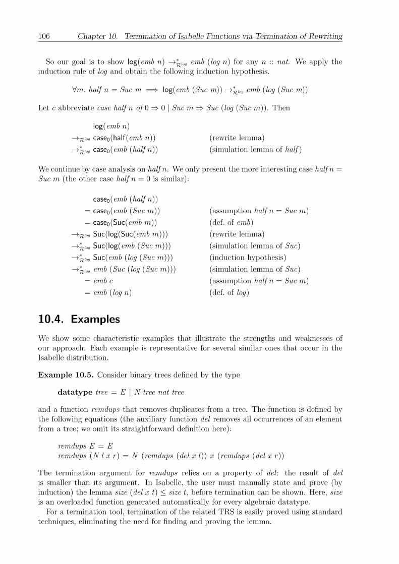
106 Chapter 10. Termination of Isabelle Functions via Termination of Rewriting
So our goal is to show log(emb n) →∗Rlog emb (log n) for any n :: nat. We apply theinduction rule of log and obtain the following induction hypothesis.
∀m. half n = Suc m =⇒ log(emb (Suc m))→∗Rlog emb (log (Suc m))
Let c abbreviate case half n of 0⇒ 0 | Suc m⇒ Suc (log (Suc m)). Then
log(emb n)
→Rlog case0(half(emb n)) (rewrite lemma)
→∗Rlog case0(emb (half n)) (simulation lemma of half )
We continue by case analysis on half n. We only present the more interesting case half n =Suc m (the other case half n = 0 is similar):
case0(emb (half n))
= case0(emb (Suc m)) (assumption half n = Suc m)
= case0(Suc(emb m)) (def. of emb)
→Rlog Suc(log(Suc(emb m))) (rewrite lemma)
→∗Rlog Suc(log(emb (Suc m))) (simulation lemma of Suc)
→∗Rlog Suc(emb (log (Suc m))) (induction hypothesis)
→∗Rlog emb (Suc (log (Suc m))) (simulation lemma of Suc)
= emb c (assumption half n = Suc m)
= emb (log n) (def. of log)
10.4. Examples
We show some characteristic examples that illustrate the strengths and weaknesses ofour approach. Each example is representative for several similar ones that occur in theIsabelle distribution.
Example 10.5. Consider binary trees defined by the type
datatype tree = E | N tree nat tree
and a function remdups that removes duplicates from a tree. The function is defined bythe following equations (the auxiliary function del removes all occurrences of an elementfrom a tree; we omit its straightforward definition here):
remdups E = Eremdups (N l x r) = N (remdups (del x l)) x (remdups (del x r))
The termination argument for remdups relies on a property of del : the result of delis smaller than its argument. In Isabelle, the user must manually state and prove (byinduction) the lemma size (del x t) ≤ size t, before termination can be shown. Here, sizeis an overloaded function generated automatically for every algebraic datatype.
For a termination tool, termination of the related TRS is easily proved using standardtechniques, eliminating the need for finding and proving the lemma.

10.5. Extensions 107
Example 10.6. The following function (originally due to Boyer and Moore [14]) normal-izes conditional expressions consisting of atoms (AT ) and if-expressions (IF ).
norm (AT a) = AT anorm (IF (AT a) y z ) = IF (AT a) (norm y) (norm z )norm (IF (IF u v w) y z ) = norm (IF u (IF v y z ) (IF w y z ))
Isabelle’s standard size measure is not sufficient to prove termination of norm, and acustom measure function must be specified by the user. Using a termination tool, theproof is fully automatic and no measure function is required.
Example 10.7. The Isabelle distribution contains the following implementation of themerge sort algorithm (transformed into non-overlapping rules internally):
msort [ ] = [ ]msort [x ] = [x ]msort xs = merge (msort (take (length xs div 2) xs)) (msort (drop (length xsdiv 2) xs))
The situation is similar to Example 10.5, as we must know how take and drop affectthe length of the list. However, in this case, Isabelle’s list theory already provides thenecessary lemmas, e.g., length (take n xs) = min n (length xs). Together with the built-inarithmetic decision procedures (which know about div and min), the termination proofworks fully automatically.
For termination tools, the proof is a bit more challenging and requires techniques thatare not yet formalized in IsaFoR (in particular, the technique of rewriting dependencypairs [37]). Thus, our connection to termination tools cannot handle msort yet. However,when this technique is added to IsaFoR in the future, no change will be required in ourimplementation to benefit from it.
These examples show the main strength of our reduction to rewriting: absolutely no userinput in the form of lemmas or measure functions is required. On the other hand, Isabelle’sability to pick up previously established results can make the built-in termination proversurprisingly strong in the presence of a good library, as the msort example shows. Eventhough that example can be solved by termination tools (and only the formalization lagsbehind), it shows an intrinsic weakness of the approach, since existing facts are not usedand must be rediscovered by the termination tool if necessary.
10.5. Extensions
In this section, we reconsider the restrictions imposed in §10.2.2.
Nested Recursion. So far, we excluded nested recursion like f (Suc n) = f (f n). Theproblem is that to prove termination of f we need its simulation lemma to reduce theinner call in the proof of the outer call, cf. §10.3.5. But proving the simulation lemmauses the induction rule of f , which in turn requires termination.
To solve this problem, we can use the partial induction rule that is generated by thefunction package even before a termination proof [69]. This rule, which is similar to theone used previously, contains extra domain conditions of the form domf x. It allows usto derive the restricted simulation lemma domf n =⇒ f(emb n) →∗Rf emb (f n). In

108 Chapter 10. Termination of Isabelle Functions via Termination of Rewriting
the termination proof obligation for the outer recursive call, we may assume this domaincondition for the inner call (a convenience provided by the function package), so that thisrestricted form of simulation lemma suffices. Hence, dealing with nested recursion simplyrequires a certain amount of additional bookkeeping.
Underspecification. So far, we require functions to be completely defined, i.e., no casesare missing in left-hand sides or case-expressions. However, head (x# xs) = x is a commondefinition. It is internally completed by head [ ] = undefined in Isabelle, where undefined ::α is an arbitrary but unknown value of type α.
For such functions, we cannot derive the simulation lemma, since this would requirehead(Nil) to be equal to emb undefined, which is an unknown term of the form Suck(0).The obvious idea of adding the rule head(Nil) → undefined to the TRS does not work,since undefined cannot be equal to emb undefined.
We can solve the problem by using fresh variables for unspecified cases, e.g., by addingthe rule head(Nil) → x. Then, the simulation lemma holds. However, the resulting TRSis no longer terminating. This new problem can be solved by using a variant of innermostrewriting, which would require support by IsaFoR as well as the termination tool.
Non-Representable Types and Polymorphism. Clearly, our embedding is limited totypes that admit a term representation. This excludes uncountable types such as realnumbers and most function types. However, even if such types occur in HOL functions,they may not be relevant for termination. Then, we can simply map all such values toa fixed constant by defining, e.g., emb (r :: real) = real. Hence, the simulation lemmasfor functions returning real numbers are trivial to prove. Furthermore, a terminationproof that does not rely on these values works without problems. Like for underspecifiedfunctions, the generated TRS no longer models the original function completely, but isonly an abstraction that is sufficient to prove termination.
A similar issue arises with polymorphic functions: To handle a function of type α list⇒α list we need a definition of emb on type α. Mapping values of type α to a constant isunproblematic, since the definition is irrelevant for the proof. However, a class instanceα :: embeddable would violate the type class discipline. This can be solved by eitherreplacing the use of type classes by explicit dictionary constructions (where emblist wouldtake the embedding function to use for the list elements as an argument), or by restrictingα to class embeddable. Since the type class does not carry any axioms, the system allowsus to remove the class constraint from the final theorem, so no generality is lost.
Higher-Order Functions. Higher-order functions pose new difficulties. First, we cannothope to define emb on function types. In particular, this means that we cannot evenstate the simulation lemma for a function like map. Second, the termination conditionsfor functions with higher-order recursion depend on user-provided congruence rules of acertain format [69]. These congruence rules then influence the form of the premise φ inthe termination condition.
A partial solution could be to create a first-order function mapf for each invocationof map on a concrete function f . Commonly used combinators like map, filter and foldcould be supported in this way.

10.6. Conclusion 109
10.6. Conclusion
We have presented a generic approach to discharge termination goals of HOL functionsby proving termination of a corresponding generated TRS. Hence, where before a man-ual termination proof might have been required, now external termination tools can beused. Since our approach is not tied to any particular termination proof technique, itspower scales up as the capabilities of termination tools increase and more techniques areformalized in IsaFoR.
A complete prototype of our implementation is available in the IsaFoR/CeTA distri-bution (version 1.18, http://cl-informatik.uibk.ac.at/software/ceta), which also includesusage examples. It remains as future work to extend our approach to a larger class ofHOL functions. Moreover, the implementation has to be more smoothly embedded intothe Isabelle system such that a user can easily access the provided functionality. Thegeneral approach is not limited to Isabelle, and could be ported to other theorem proverslike Coq, which has similar recursive definition facilities (e.g., [6]) and rewriting librariessimilar to IsaFoR [13, 21].
Acknowledgment. Jasmin Blanchette gave helpful feedback on a draft of this paper.


11. Generalized and FormalizedUncurrying
Publication details
Christian Sternagel and Rene Thiemann. Generalized and Formalized Uncurrying. InProceedings of the 8th International Symposium on the Frontiers of Combining Systems,volume 6989 of LNCS, pages 243–258. Springer, 2011.
Abstract
Uncurrying is a termination technique for applicative term rewrite systems. During ourformalization of uncurrying in the theorem prover Isabelle, we detected a gap in theoriginal pen-and-paper proof which cannot directly be filled without further precondi-tions. Our final formalization does not demand additional preconditions, and generalizesthe existing techniques since it allows to uncurry non-applicative term rewrite systems.Furthermore, we provide new results on uncurrying for relative termination and for de-pendency pairs.
11.1. Introduction
In recent years, the way to prove termination of term rewrite systems (TRSs) has changed.Current termination tools no longer search for a single reduction order containing therewrite relation. Instead, they combine various termination techniques in a modular way,resulting in large and tree-like termination proofs, where at each node a specific techniqueis applied.
On the one hand, this combination makes termination tools more powerful. On theother hand, it makes them more complex and error-prone. It is regularly demonstratedthat we cannot blindly trust the output of termination provers. Every now and then,some prover delivers a faulty proof. Often, this is only detected if there is another provergiving a contradictory answer for the same input, as a manual inspection of proofs isinfeasible due to their size.
The problem is solved by combining two systems. For a given TRS, we first use atermination tool to automatically detect a termination proof (which may contain errors).Then, we use a highly trusted certifier which checks whether the detected proof is indeedcorrect. In total, the combination yields a powerful and trustable workflow to provetermination.
To obtain a highly trustable certifier, a common approach is to first formalize thedesired termination techniques once and for all (thereby ensuring their soundness) andthen, for a given proof, check that the used techniques are applied correctly [12, 23,104]. We formalized the dependency pair framework (DP framework) [42] and manytermination techniques in our Isabelle/HOL [84] library IsaFoR [104] (in the remainder

112 Chapter 11. Generalized and Formalized Uncurrying
we just write Isabelle, instead of Isabelle/HOL). From IsaFoR, we code-extract CeTA, anautomatic certifier for termination proofs.
In this paper, we present one of the latest additions to IsaFoR: the formalization ofuncurrying, as described in [53]. However, we did not only formalize uncurrying, but alsogeneralized it. Furthermore, we found a gap in one of the original proofs, which we couldfortunately close.
Note that all the proofs that are presented (or omitted) in the following, have beenformalized as part of IsaFoR. Hence, in this paper, we merely give sketches of our “real”proofs. Our goal is to show the general proof outlines and help to understand the fullproofs. The library IsaFoR with all formalized proofs, the executable certifier CeTA, and alldetails about our experiments are available at CeTA’s website: http://cl-informatik.
uibk.ac.at/software/ceta.
The paper is structured as follows. In Sect. 11.2, we shortly recapitulate some requirednotions of term rewriting. Afterwards, in Sect. 11.3, we describe applicative rewriting,give an overview of approaches using uncurrying for proving termination, and present ourgeneralization of uncurrying for TRSs. Then, in Sect. 11.4, we show how to lift uncurryingto the DP framework. We present heuristics and our experiments in Sect. 11.5, before weconclude in Sect. 11.6.
11.2. Preliminaries
We assume familiarity with term rewriting [5]. Still, we recall the most important notionsthat are used later on. A (first-order) term t over a set of variables V and a set of(function) symbols F is either a variable x ∈ V or a function symbol f ∈ F applied toargument terms f(t1, . . . , tn) where the arity of f is ar(f) = n. A context C is a termcontaining exactly one hole 2. Replacing 2 in a context C by a term t is denoted by C[t].
A rewrite rule is a pair of terms `→ r and a TRS R is a set of rewrite rules. The setof defined symbols (of R) is DR = {f | f(. . .) → r ∈ R}. The rewrite relation (inducedby R) →R is the closure under substitutions and contexts of R, i.e., s →R t iff there isa context C, a rewrite rule ` → r ∈ R, and a substitution σ such that s = C[`σ] andt = C[rσ]. A term t is root-stable w.r.t. R iff there is no derivation t →∗R `σ for some`→ r ∈ R and substitution σ.
We say that a term t is terminating w.r.t. R (SNR(t)) if it cannot start an infinitederivation t = t1 →R t2 →R t3 →R · · · . A TRS is terminating (SN(R)) iff all terms areterminating w.r.t. R. A TRS R is terminating relative to a TRS S iff there is no infiniteR∪ S-derivation with infinitely many R-steps.
11.3. Applicative Rewriting and Uncurrying
An applicative term rewrite system (ATRS) is a TRS over an applicative signature F ={◦} ∪ C, where ◦ is a unique binary symbol (the application symbol) and all symbolsin C are constants. ATRSs can be used to encode many higher-order functions withoutexplicit abstraction as first-order TRSs. In the remainder we use ◦ as an infix-symbolwhich associates to the left (s ◦ t ◦ u = (s ◦ t) ◦ u). In examples we omit ◦ whenever thisincreases readability.

11.3. Applicative Rewriting and Uncurrying 113
Example 11.1. The following ATRS R (a variant of [53, Example 7], replacing additionby subtraction) contains the map function (which applies a function to all arguments ofa list) and subtraction on Peano numbers in applicative form.
1: sub 0 → K 02: sub x 0 → x3: sub x x → 04: sub (s x) (s y) → sub x y
5: K x y → x6: map z nil → nil7: map z (cons x xs) → cons (z x) (map z xs)
Proving termination of ATRSs is challenging without dedicated termination techniques(e.g., for reduction orders, we cannot interpret sub ◦x ◦ y as x, since sub is a constant andnot binary).
Until now, there have at least been three approaches to tackle this problem. All of themtry to uncurry a TRS such that, for example, Rule 4 from above becomes sub(s(x), s(y))→sub(x, y).
To distinguish the three approaches, we need the following definitions:
Definition 11.2. A term t is head variable free iff t does not contain a subterm of theform x ◦ s where x is a variable. The applicative arity of a constant f in an ATRS R(aaR(f)) is the maximal number n, such that f ◦ t1 ◦ · · · ◦ tn occurs as a subterm in R.Uncurrying an application f ◦ t1 ◦ · · · ◦ tn with aaR(f) = n yields the term f(t1, . . . , tn).A term t is proper w.r.t. aaR iff t is a variable or t = f ◦ t1 ◦ · · · ◦ tn where aaR(f) = nand each ti is proper.
The oldest of the three approaches is from [59]. It requires that all terms in a TRSare proper w.r.t. aaR, and shows that then termination of R is equivalent to terminationof the TRS obtained by uncurrying all terms of R. Since proper terms do not containany partial applications, the application symbol is completely eliminated by uncurrying.However, requiring proper terms is rather restrictive: Essentially, it is demanded that theTRS under consideration is a standard first-order TRS which is just written in applicativeform. For example, the approach is not applicable to Example 11.1, since there is a headvariable in the right-hand side of Rule 7 (z ◦x) and sub as well as K are applied to a singleargument in Rule 1, even though aaR(sub) = 2 and aaR(K) = 2.
The second approach was given in [41, 101]. Here, the same preconditions as in [59]apply, but the results are extended to innermost rewriting and to the DP framework. Thelatter has the advantage, that only the current subproblem has to satisfy the preconditions.For example, when treating the dependency pair
map ◦ z ◦] (cons ◦ x ◦ xs)→ map ◦ z ◦] xs (1)
for the recursive call of map, we can perform uncurrying (since there are no usable rulesand (1) satisfies the preconditions). Moreover, in [101] uncurrying is combined with thereduction pair processor to further relax the preconditions.
The third approach is given in [53]. Here, the preconditions for uncurrying have beenreduced drastically as only the left-hand sides of the TRS R must be head variable free.In return, we have to η-saturate R and add uncurrying rules. Moreover, for each constantf with aaR(f) = n we obtain n new function symbols f1, . . . , fn of arities 1, 2, . . . , n whichhandle partial applications.
Example 11.3. When η-saturating the TRS R of Example 11.1, we have to add the rulesub ◦ 0 ◦ y → K ◦ 0 ◦ y. The uncurried TRS consists of the following rules:

114 Chapter 11. Generalized and Formalized Uncurrying
8: sub1(0) → K1(0)9: sub2(0, y) → K2(0, y)
10: sub2(x, 0) → x11: sub2(x, x) → 0
12: sub2(s1(x), s1(y)) → sub2(x, y)13: K2(x, y) → x14: map2(z, nil) → nil15: map2(z, cons2(x, xs)) → cons2(z ◦ x,map2(z, xs))
Moreover, we have to add the following uncurrying rules:
16: s ◦ x → s1(x)17: K ◦ x → K1(x)18: K1(x) ◦ y → K2(x, y)19: sub ◦ x → sub1(x)20: sub1(x) ◦ y → sub2(x, y)
21: cons ◦ x → cons1(x)22: cons1(x) ◦ y → cons2(x, y)23: map ◦ x → map1(x)24: map1(x) ◦ y → map2(x, y)
Also [53] gives an extension to the DP framework.To summarize, the traditional technique of uncurrying of [59] is completely subsumed
by [41, 101], but [41, 101] and [53] are incomparable. The advantage of [41, 101] is thatthe generated TRSs and DP problems are smaller, and that uncurrying is also availablein a combination with the reduction pair processor, whereas [53] supports head variables(see [101, Chap. 6] for a more detailed comparison).
Since [53] is used in more termination tools (it is used in at least Jambox [31] and TTT2[67] whereas we only know of AProVE [39] that implements all uncurrying techniques of[41,101]), we incorporated the techniques of [53] in our certifier CeTA.
During our formalization we have
• detected a gap in a proof of [53] which could not directly be closed without addingfurther preconditions to one of the main results,
• generalized the technique of uncurrying which now entails the result of [53] evenwithout adding any additional precondition, and
• generalized the technique of freezing from [53].
The structure in [53] is as follows. First, uncurrying is developed for TRSs over ap-plicative signatures {◦} ∪ C. Then, it is extended to DP problems, introducing a secondapplication symbol ◦] that may only occur at root-positions of P and is not uncurried atall. Finally, freezing is applied to uncurry applications of ◦].
Following this structure, we first fully formalized uncurrying on TRSs. However, inthe extension to DP problems there is a missing step which is illustrated in more detailin Example 11.14 on page 119. The main problem is that signature restrictions on DPproblems are in general unsound.
To fill the gap, one option is to use the results of [97] about signature restrictions, whichcan however only be applied if R is left-linear. This clearly weakens the applicability ofuncurrying, e.g., Example 11.1 is not left-linear.
Alternatively, one can try to perform uncurrying without restricting to applicativesignatures. This is what we did. All uncurrying techniques that we formalized work onterms and TRSs over arbitrary signatures.
The major complication is the increase of complexity in the cases that have to beconsidered. For example, using an applicative signature, we can assume that every termis of the form x ◦ t1 ◦ · · · ◦ tn or f ◦ t1 ◦ · · · ◦ tn where n ∈ N, x is a variable, and f isa constant. Generalizing this to arbitrary signatures we have to consider the two casesx ◦ t1 ◦ · · · ◦ tn and f(s1, . . . , sm) ◦ t1 ◦ · · · ◦ tn instead, where f is an m-ary symbol. Hence,

11.3. Applicative Rewriting and Uncurrying 115
when considering a possible rewrite step, we also have to consider the new case that thestep is performed in some si.
We not only generalized uncurrying to work for arbitrary signatures and relative rewrit-ing, but also to a free choice of the applicative arity aa(f). This is in contrast to [53],where the applicative arity is fixed by Definition 11.2. We will elaborate on this differenceafter presenting our main theorem.
Definition 11.4 (Symbol maps and applicative arity). Let F be a signature. A symbolmap is a mapping π : F → [F ] from symbols to non-empty lists of symbols. It is injectiveif for all f and g, π(f) contains no duplicates, π(f) does not contain ◦, and wheneverf 6= g then π(f) and π(g) do not share symbols. If π(f) = [f0, . . . , fn], then the applicativearity of f w.r.t. π is aaπ(f) = n. The applicative arity of a term is defined by aaπ(t) =aaπ(f) .−n, where x .−y = max(x−y, 0), for t = f(s1, . . . , sm)◦t1◦· · ·◦tn and is undefinedotherwise.
Intuitively, if π(f) = [f0, . . . , fn] then every application of f on i 6 n argumentst1, . . . , ti will be fully uncurried to fi(t1, . . . , ti). If more than n arguments are applied,then we obtain fn(t1, . . . , tn) ◦ tn+1 ◦ . . . ◦ ti. A symbol map containing an entry for f ,uniquely determines the applicative arity n as well as the names of the (partial) applica-tions f0, . . . , fn of f .
In the following we assume a fixed symbol map π and just write aa(f) and aa(t) insteadof aaπ(f) and aaπ(t), respectively. Additionally, we assume that π(f) = [f0, . . . , faa(f)]where in examples we write f instead of f0. Now we can define the uncurrying TRS w.r.t.π.
Definition 11.5. The uncurrying TRS U contains the rule
fk(x1, . . . , xm, y1, . . . , yk) ◦ yk+1 → fk+1(x1, . . . , xm, y1, . . . , yk+1)
for every f ∈ F with ar(f) = m and aa(f) = n, and every k < n. The variables x1, . . . ,xm, y1, . . . , yk+1 are pairwise distinct.
In [53], terms are uncurried by computing the unique normal form w.r.t. U . For ourformalization we instead used the upcoming uncurrying function for the following tworeasons: First, we do not have any results about confluence of TRSs. Hence, to evendefine the normal form w.r.t. U would require to formalize several additional lemmaswhich show that every term has exactly one normal form. This would be quite someeffort which we prefer to avoid. The second reason is efficiency. When certifying theapplication of uncurrying in large termination proofs, we have to compute the uncurriedversion of a term. It is just more efficient to use a function which performs uncurryingdirectly, than to compute a normal form w.r.t. a TRS where possible redexes have to besearched, etc.
Definition 11.6. The uncurrying function x·y on terms is defined as
• xx ◦ t1 ◦ · · · ◦ tny = x ◦ xt1y ◦ · · · ◦ xtny
• xf(s1, . . . , sm) ◦ t1 ◦ · · · ◦ tny = fk(xs1y, . . . , xsmy, xt1y, . . . , xtky)◦xtk+1y◦ · · · ◦xtnywhere k = min(n, aa(f))
It is homomorphically extended to operate on rules, TRSs, and substitutions.

116 Chapter 11. Generalized and Formalized Uncurrying
We establish the link between U and x·y in the following lemma which generalizes thecorresponding results in [53].
Lemma 11.7.
• if k < aa(f) and ar(f) = m then fk(s1, . . . , sm+k) ◦ t→U fk+1(s1, . . . , sm+k, t)
• if k + n 6 aa(f) and ar(f) = m then fk(s1, . . . , sm+k) ◦ t1 ◦ . . . ◦ tn →∗U fk+n(s1, . . . ,sm+k, t1, . . . , tn)
• xsy ◦ xt1y ◦ · · · ◦ xtny→∗U xs ◦ t1 ◦ · · · ◦ tny
• if aa(s) = 0 or aa(s) is undefined then xs ◦ t1 ◦ · · · ◦ tny = xsy ◦ xt1y ◦ · · · ◦ xtny
• xsy · xσy→∗U xs · σy
• if t is head variable free then xs · σy = xsy · xσy
The last two results show how uncurrying can be exchanged with applying substitutions.As we will often need the equality x` · σy = x`y · xσy for left-hand sides `, it is naturallyto demand that left-hand sides are head variable free.
Definition 11.8. A TRS is left head variable free if all left-hand sides are head variablefree.
Termination of xRy∪U does not suffice to conclude termination of R, cf. [53, Example13]. The reason is that first we have to η-saturate R.
Definition 11.9. A TRS R is η-closed iff for every rule `→ r with aa(`) > 0 there is arule `◦x→ r ◦x ∈ R where x is fresh w.r.t. `→ r. The η-saturation Rη of R is obtainedby adding new rules ` ◦ x→ r ◦ x until the result is η-closed.
The upcoming theorem is the key to use uncurrying for termination proofs. It allowsto simulate one R-step by many steps in the uncurried system.
Theorem 11.10. Let R be η-closed and left head variable free. Let there be no left-handside of R which is a variable. If s→R t then xsy→+
xRy∪U xty.
Proof. Let s = C[`σ] →R C[rσ] = t where ` → r ∈ R. We show xsy →+xRy∪U xty by
induction on the size of C.
• If C = f(s1, . . . , D, . . . , sm) ◦ t1 ◦ · · · ◦ tn for some f 6= ◦ then by the inductionhypothesis we know that xD[`σ]y→+
xRy∪U xD[rσ]y. Moreover,
xsy = xf(s1, . . . , D[`σ], . . . , sm) ◦ t1 ◦ · · · ◦ tny= fk(xs1y, . . . , xD[`σ]y, . . . , xsmy, xt1y, . . . , xtky) ◦ xtk+1y ◦ · · · ◦ xtny→+
xRy∪U fk(. . . , xD[rσ]y, . . . , xsmy, xt1y, . . . , xtky) ◦ xtk+1y ◦ · · · ◦ xtny= xf(s1, . . . , D[rσ], . . . , sm) ◦ t1 ◦ · · · ◦ tny= xty
where k = min(n, aa(f)).

11.3. Applicative Rewriting and Uncurrying 117
• If C = t0◦D◦ t1◦· · ·◦ tn then by the induction hypothesis we know xD[`σ]y→+xRy∪U
xD[rσ]y. If aa(t0) = 0 or aa(t0) is undefined then
xsy = xt0 ◦D[`σ] ◦ t1 ◦ · · · ◦ tny= xt0y ◦ xD[`σ]y ◦ xt1y ◦ · · · ◦ xtny→+
xRy∪U xt0y ◦ xD[rσ]y ◦ xt1y ◦ · · · ◦ xtny= xt0 ◦D[rσ] ◦ t1 ◦ · · · ◦ tny= xty
Otherwise, aa(t0) > 0 and hence, t0 = f(s1, . . . , sm) ◦ sm+1 ◦ · · · ◦ sm+k wherek < aa(f). It follows that
xsy = xf(s1, . . . , sm) ◦ sm+1 ◦ · · · ◦ sm+k ◦D[`σ] ◦ t1 ◦ · · · ◦ tny= fk+1+n′(. . . , xsm+ky, xD[`σ]y, xt1y, . . . , xtn′y) ◦ xtn′+1y ◦ · · · ◦ xtny→+
xRy∪U fk+1+n′(. . . , xsm+ky, xD[rσ]y, xt1y, . . . , xtn′y) ◦ xtn′+1y ◦ · · ·= xf(s1, . . . , sm) ◦ sm+1 ◦ · · · ◦ sm+k ◦D[rσ] ◦ t1 ◦ · · · ◦ tny= xty
where n′ = min(aa(f)− k − 1, n).
• If C = 2 ◦ t1 ◦ · · · ◦ tn and n = 0 ∨ aa(`) = 0 then
xsy = x` · σ ◦ t1 ◦ · · · ◦ tny= x` · σy ◦ xt1y ◦ · · · ◦ xtny= x`y · xσy ◦ xt1y ◦ · · · ◦ xtny→xRy xry · xσy ◦ xt1y ◦ · · · ◦ xtny→∗U xr · σy ◦ xt1y ◦ · · · ◦ xtny→∗U xr · σ ◦ t1 ◦ · · · ◦ tny= xty
since ` is head variable free and if n 6= 0 then aa(`σ) = aa(`) = 0.
• If C = 2◦t1◦· · ·◦tn with n > 0 and aa(`) > 0 then `′ → r′ = `◦x→ r◦x ∈ R sinceR is η-closed. Moreover, by changing σ to δ = σ ] {x/t1} we achieve s = ` · σ ◦ t1 ◦· · ·◦ tn = `′δ◦ t2 ◦· · ·◦ tn = D[`′δ] and r = r ·σ◦ t1 ◦· · ·◦ tn = r′δ◦ t2 ◦· · ·◦ tn = D[r′δ]for the context D = 2◦ t2 ◦ · · · tn which is strictly smaller than C. Hence, the resultfollows by the induction hypothesis.
• If C = 2◦ t1 ◦ · · · ◦ tn with n > 0 and aa(`) is undefined then ` = x◦ `1 ◦ · · · ◦ `k withk ≥ 0. But if k > 0 then ` is not head variable free and if k = 0 then R contains avariable as left-hand side. In both cases we get a contradiction to the preconditionsin the theorem.
Note that the condition that the left-hand sides of R are not variables is new in com-parison to [53]. Nevertheless, in the following corollary we can drop this condition, sinceotherwise xRy is not terminating anyway.
Corollary 11.11. If Rη is left head variable free then termination of xRηy ∪ U impliestermination of R.

118 Chapter 11. Generalized and Formalized Uncurrying
When using uncurrying for relative termination of R/S, it turns out that the newcondition on the left-hand sides can only be ignored for R – since otherwise relativetermination of xRy/xSy ∪ U does not hold – but not for S.
Corollary 11.12. If Rη ∪ Sη is left head variable free and the left-hand sides of S arenot variables, then relative termination of xRηy/xSηy∪U implies relative termination ofR/S.
Example 11.13. Let R = {f ◦ f ◦ x → f ◦ x} and S = {x → f ◦ x}. Then R/S is notrelative terminating since f◦f◦x→R f◦x→S f◦f◦x→R . . . is an infiniteR∪S-derivationwith infinitely many R-steps.
For π(f) = [f, f1, f2] we have Rη = R, Sη = S, xRηy = {f2(f, x)→ f1(x)}, xSηy = {x→f1(x)}, and U = {f ◦ x→ f1(x), f1(x) ◦ y → f2(x, y)}. It is easy to see that xRηy/xSηy∪Uis relative terminating by counting the number of f-symbols. Since both Rη and Sη arehead variable free, we have shown that Corollary 11.12 does not hold if one would dropthe new variable condition on S.
As already mentioned, Corollary 11.11 generalizes the similar result of [53, Theorem 16]in two ways: first, there is no restriction to applicative signatures, and second, one canfreely choose the applicative arities. Since in principle the choice of π does not matter(uncurrying preserves termination for every choice of π), we can only heuristically deter-mine whether the additional freedom increases termination proving power and thereforerefer to our experiments in Sect. 11.5.
11.4. Uncurrying in the Dependency Pair Framework
The DP framework [42] facilitates modular termination proofs. Instead of single TRSs, weconsider DP problems (P ,R), consisting of two TRSs P and R where elements of P areoften called pairs to distinguish them from the rules of R. The initial DP problem for aTRS R is (DP(R),R), where DP(R) = {f ](s1, . . . , sn)→ g](t1, . . . , tm) | f(s1, . . . , sn)→C[g(t1, . . . , tm)] ∈ R, g ∈ DR} is the set of dependency pairs of R, incorporating a freshtuple symbol f ] for each defined symbol f . The initial DP problem is also a standard DPproblem, i.e., root symbols of pairs do not occur elsewhere in P or R.1 A (P ,R)-chainis a possibly infinite derivation of the form:
s1σ1 →P t1σ1 →∗R s2σ2 →P t2σ2 →∗R s3σ3 →P · · · (?)
where si → ti ∈ P for all i > 0. If additionally every tiσi is terminating w.r.t. R,then the chain is minimal. A DP problem (P ,R) is called finite [42], if there is nominimal infinite (P ,R)-chain. Proving finiteness of a DP problem is done by simplifying(P ,R) using so called processors recursively. A processor transforms a DP problem into anew DP problem. The aim is to reach a DP problem with empty P-component (such DPproblems are trivially finite). To conclude finiteness of the initial DP problem, the appliedprocessors need to be sound. A processor Proc is sound whenever for all DP problems(P ,R) we have that finiteness of Proc(P ,R) implies finiteness of (P ,R).
In the following we explain how uncurrying is used as processor in the DP framework.In Sect. 11.3 it was already mentioned that in [53] the notion of applicative TRS waslifted to applicative DP problem by allowing a new binary application symbol ◦] (where
1Several termination provers only work on standard DP problems.

11.4. Uncurrying in the Dependency Pair Framework 119
we sometimes just write ] in examples). The symbol ◦] naturally occurs as tuple symbolof ◦.
To prove soundness of the uncurrying processor, in [53] it is assumed that there is aminimal (P ,R)-chain s1σ1 →P t1σ1 →∗R s2σ2 →P · · · , which is converted into a minimal(xPy, xRηy ∪ U)-chain by reusing the results for TRSs. However, there is a gap in thisreasoning. Right in the beginning it is silently assumed that all terms siσi and tiσi havetuple symbols as roots and that their arguments are applicative terms, i.e., terms overan applicative signature {◦} ∪ C. Without this assumption it is not possible to apply theresults of uncurrying for TRSs, since those are only available for applicative terms in [53].
The following variant of [97, Example 14] shows that in general restricting substitutionsin chains to an applicative signature {◦} ∪ C is unsound.
Example 11.14. Consider the applicative and standard DP problem (P ,R) where P ={g ] (f x y z z u v)→ g ] (f x y x y x (h y u))} and R contains the rules:
a → ba → c
h x x → h x x
f a x2 x3 x4 x5 → f a x2 x3 x4 x5f x1 a x3 x4 x5 → f x1 a x3 x4 x5
f (y z) x2 x3 x4 x5 → f (y z) x2 x3 x4 x5f x1 (y z) x3 x4 x5 → f x1 (y z) x3 x4 x5
There is a minimal (P ,R)-chain taking si = g](f x y z z u v), ti = g] (f x y x y x (h y u)),and σi = {x/k(a), y/k(b), z/k(b), u/k(c), v/h (k(b)) (k(c))} where k is a unary symbol.However, there is no minimal (P ,R)-chain using substitutions over the signature {◦}∪C,regardless of the choice of constants C.
Since our generalizations in Sect. 11.3 do not have any restrictions on the signature, wewere able to correct the corresponding proofs in [53] such that the major theorems arestill valid.2 It follows the generalization of [53, Theorem 33].
Theorem 11.15. The uncurrying processor U ′1 is sound where U ′1(P ,R) ={(xPy, xRηy ∪ U) if P ∪Rη is left head variable free and π is injective,
(P ,R) otherwise.
Proof. The proof mainly uses the results from the previous section. We assume an infiniteminimal (P ,R)-chain s1σ1 →P t1σ1 →∗R s2σ2 →P t2σ2 →∗R · · · and construct an infiniteminimal (xPy, xRηy ∪ U)-chain as follows.
We achieve xsiσiy = xsiy · xσiy and xtiy · xσiy →∗U xtiσiy since P is left head variablefree. Moreover, using tiσi →∗R si+1σi+1 and Theorem 11.10 we conclude xtiσiy →∗xRηy∪Uxsi+1σi+1y. Here, the condition that Rη must not contain variables as left-hand sides isensured by the minimality of the chain: if x → r ∈ Rη then SNR(tiσ) does not hold.Hence, we constructed a (xPy, xRηy ∪ U)-chain as
xsiσiy = xsiy · xσiy→xPy xtiy · xσiy→∗U xtiσiy→∗xRηy∪U xsi+1σi+1y
for all i. To ensure that the chain is minimal it is demanded that π is injective. Otherwise,two different symbols can be mapped to the same new symbol which clearly can introducenontermination. The structure of the proof that minimality is preserved is similar to theone in [53] and we just refer to IsaFoR for details.
2After the authors of [53] where informed of the gap, they independently developed an alternative fix,which is part of an extended, but not yet published version of [53].

120 Chapter 11. Generalized and Formalized Uncurrying
The uncurrying processor of Theorem 11.15 generalizes [53, Theorem 33] in three ways:the signature does not have to be applicative, we can freely choose the applicative arityvia π, and we can freely choose the application symbol. The last generalization letsTheorem 11.15 almost subsume the technique of freezing [53, Corollary 40] which is usedto uncurry ◦].
Definition 11.16 (Freezing [53]). A simple freeze f is a subset of F .3 Freezing is appliedon non-variable terms as follows
f(f(t1, . . . , tn)) =
{f(t1, . . . , tn) if n = 0 or f /∈ f
f g(s1, . . . , sm, t2, . . . , tm) if t1 = g(s1, . . . , sm) and f ∈ f
where each f g is a new symbol. It is homomorphically extended to rules and TRSs. Thefreezing DP processor is defined as f(P ,R) =
(f(P),R) if (P ,R) is a standard DP problem where for all s→ f(t1, . . . , tn)
∈ P with f ∈ f, both t1 /∈ V and all instances of t1 are root-stable,
(P ,R) otherwise.
In [53, Theorem 39], it is shown that freezing is sound.
Example 11.17. In the following we use numbers to refer to rules from previous examples.We consider the DP problem (P ,R) where P = {sub (s x) ] (s y) → sub x ] y} andR = {2–4}. Uncurrying ◦ with π(s) = [s, s1], π(sub) = [sub, sub1, sub2], π(0) = [0], andπ(]) = []] yields the DP problem (xPy, xRηy ∪ U) where xPy = {sub1(s1(x)) ] s1(y) →sub1(x) ] y} and xRηy ∪ U consists of {10–12, 16, 19, 20}.
Afterwards we uncurry the resulting DP problem using ◦] as application symbol and πwhere π(sub1) = [sub1,−]] and π(f) = [f ] for all other symbols. We obtain (P ′,R′) whereP ′ = {s1(x) −] s1(x)) → x −] y} and R′ = xRηy ∪ U ∪ {sub1(x) ] y → −](x, y)}. Notethat freezing returns nearly the same DP problem. The only difference is that uncurryingproduces the additional rule sub1(x) ] y → x −] y which we do not obtain via freezing.However, since this rule is not usable it also does not harm that much.
Moreover, uncurrying sometimes is applicable where freezing is not. If we would havestarted with the DP problem (P ,R′′) where R′′ = {1–5} then uncurrying would resultin (xPy, xR′′ηy ∪ U ′) where xR′′ηy ∪ U ′ = {8–13, 16–20}. On this DP problem freezingis not applicable (the instances of sub1(x) in the right-hand side of the only pair inxPy are not root-stable due to Rule 8). Nevertheless, one can uncurry ◦], resulting in(P ′, xR′′ηy ∪ U ′ ∪ Rnew) where Rnew = {sub1(x) ] y → x −] y, 0 −] y → K1(0) ] y}. Notethat the uncurrying of ◦] transformed a standard DP problem into a non-standard one,as −] occurs as root of a term in P ′, but also within Rnew.
Whenever freezing with f = {◦]} is applicable, then also uncurrying of ◦] is possible:the condition t1 /∈ V in Definition 11.16 implies that P ∪ Rη is left head variable free.The only difference is that uncurrying produces more rules than freezing, namely theuncurrying rules and the uncurried rules of those rules which have to be added for theη-saturation. However, if freezing is applicable then none of these additional rules are
3In [53] one can also specify an argument position for each symbol. This can be simulated by permutingthe arguments accordingly.

11.4. Uncurrying in the Dependency Pair Framework 121
usable.4 Hence, all techniques which only consider the usable rules (like the reduction pairprocessor) perform equally well, no matter whether one has applied freezing or uncurrying.Still, one wants to get rid of the additional rules, especially since they are also the reasonwhy standard DP problems are transformed into non-standard ones.
In Example 11.17 we have seen that sometimes uncurrying of tuple symbols is applica-ble where freezing is not. Thus, to have the best of both techniques we devised a specialuncurrying technique for tuple symbols which fully subsumes freezing without the disad-vantage of U ′1: if freezing is applicable then standard DP problems are transformed intostandard DP problems by the new technique.
Before we describe the new uncurrying processor formally, we shortly list the differencesto the uncurrying processor of Theorem 11.15:
• Since the task is to uncurry tuple symbols, we restrict the applicative arities to beat most one. Moreover, uncurrying is performed only on the top-level. Finally, theapplication symbol may be of arbitrary non-zero arity.
• Rules that have to be added for the η-saturation and the uncurrying rules are addedas pairs (to the P-component), and not as rules (to the R-component).
• If freezing is applicable, we do neither add the uncurrying rules nor do we applyη-saturation.
Example 11.18. We continue with the DP problems of Example 11.17.If one applies the special uncurrying processor on (xPy, xRηy ∪ U) then one obtains
(P ′, xRηy ∪ U) which is the same as f(xPy, xRηy ∪ U) for f = {◦]}.And if one applies the special uncurrying processor on (xPy, xR′′ηy∪U ′) then one obtains
the standard DP problem (P ′ ∪Rnew, xR′′ηy ∪ U ′).
Definition 11.19. Let ◦] be an n-ary application symbol where n > 0. Let π be aninjective symbol map where π(f) ∈ {[f ], [f, f ]]} for all f . The top-uncurrying functionp·q maps terms to terms. It is defined as ptq ={
f ](s1, . . . , sm, t2, . . . , tn) if t = ◦](f(s1, . . . , sm), t2, . . . , tn) and π(f) = [f, f ]]
t otherwise
and is homomorphically extended to pairs, rules, and substitutions. The top-uncurryingrules are defined as
U t = {◦](f(x1, . . . , xm), y2, . . . , yn)→ f ](x1, . . . , xm, y2, . . . , yn) | π(f) = [f, f ]]}
Then the top-uncurrying processor is defined as top(P ,R) =(pPηq ∪ U t?,R) if ◦] is not defined w.r.t. R and for all s→ t ∈ Pη : s, t /∈ V,
s 6= ◦](x, s2, . . . , sn), and the root of t is not defined w.r.t. R(P ,R) otherwise
where U t? = ∅ and Pη = P if for all s → ◦](t1, . . . , tn) ∈ P and σ the term t1σ isroot-stable, and U t? = U t and Pη = P ∪ {◦](`, x2, . . . , xn) → ◦](r, x2, . . . , xn) | ` → r ∈R, root(`) = g, π(g) = [g, g]]}, otherwise. Here, x2, . . . , xn are distinct fresh variables thatdo not occur in `→ r.4In detail: a technique that can detect that instances of a subterm of a right-hand side of P are root-
stable can also detect that the additional rules are not usable.

122 Chapter 11. Generalized and Formalized Uncurrying
Theorem 11.20. The top-uncurrying processor top is sound.
Proof. The crucial part is to prove that whenever t = f(t1, . . . , tm) →∗R s, f /∈ DR, tis an instance of a right-hand side of P , and SNR(t), then ptq →∗pPηq∪Ut?∪R psq where
pPηq ∪ U t?-steps are root steps and all terms in this derivation are terminating w.r.t. R.Using this result, the main result is established as follows. Assume there is an infinite
minimal (P ,R)-chain. Then every step sσ →P tσ →∗R s′σ′ in the chain is transformedas follows. Since s → t ∈ P , we conclude that tσ = f(t1σ, . . . , tmσ) where f /∈ DR andSNR(tσ). Hence, using the crucial step we know that ptσq→∗pPηq∪Ut?∪R ps′σ′q. Moreover,
by case analysis on t one can show that ptqσ →∗Ut? ptσq via root reductions, and similarly,
by additionally using the restrictions on s one derives psσq = psqσ. Hence,
psσq = psqσ →pPq ptqσ →∗Ut? ptσq→∗pPηq∪Ut?∪R
ps′σ′q
where all terms in this derivation right of →pPq are terminating w.r.t. R and where allpPηq ∪ U t?-steps are root reductions. Thus, we can turn the root reductions into pairs,resulting in an infinite minimal (pPηq ∪ U t?,R)-chain.
To prove the crucial part we perform induction on the number of steps where the basecase – no reductions – is trivial. Otherwise, t = f(t1, . . . , tm)→∗R u→R s. Using SNR(t)we also know SNR(u) and since f /∈ DR we know that u = f(u1, . . . , um) and ti →∗R uifor all 1 6 i 6 m. Moreover, s = f(s1, . . . , sm) and s is obtained from u by a reductionui →R si for some 1 6 i 6 m. Hence, we may apply the induction hypothesis andconclude ptq→∗pPηq∪Ut?∪R puq.
It remains to simulate the reduction u →R s. The simulation is easy if f 6= ◦], sincethen puq = u →R s = psq. Otherwise, f = ◦] and m = n. We again first considerthe easy case where ui →R si for some i > 1. Then an easy case analysis on u1 yieldspuq →R psq since u and s are uncurried in the same way (since u1 = s1). Otherwise,u = ◦](u1, . . . , um), s = ◦](s1, u2, . . . , um) and u1 →R s1. If u1 →R s1 is a reduction belowthe root then both s and t are uncurried in the same way and again puq→R psq is easilyestablished. If however u1 = `σ → rσ = s1 for some rule `→ r ∈ R then we know that u1is not root-stable and hence also t1 is not root-stable. As t = ◦](t1, . . . , tn) is an instanceof a right-hand side of P we further know that there is a pair s′ → ◦](t′1, . . . , t′n) ∈ Pwhere t1 = t′1σ. Since t′1σ is not root-stable U t? = U t and Pη ⊇ {◦](`, x2, . . . , xn) →◦](r, x2, . . . , xn) | ` → r ∈ R, root(`) = g, π(g) = [g, g]]}. Let ` = g(`1, . . . , `k). Ifπ(g) = [g] then
puq = p◦](g(`1, . . . , `k)σ, u2, . . . , un)q
= ◦](g(`1, . . . , `k)σ, u2, . . . , un)
→R ◦](rσ, u2, . . . , un)
→∗Ut? p◦](rσ, u2, . . . , un)q
= psq.
And otherwise, π(g) = [g, g]]. Hence, ◦](`, x2, . . . , xn)→ ◦](r, x2, . . . , xn) ∈ Pη. We defineδ = σ ] {x2/u2, . . . , xn/un} and achieve
puq = p◦](g(`1, . . . , `k)σ, u2, . . . , un)q
= g](`1σ, . . . , `kσ, u2, . . . , un)
= g](`1, . . . , `k, x2, . . . , xn)δ
= p◦](g(`1, . . . , `k), x2, . . . , xn)qδ

11.5. Heuristics and Experiments 123
= p◦](`, x2, . . . , xn)qδ
→pPηq p◦](r, x2, . . . , xn)qδ
→∗Ut? p◦](r, x2, . . . , xn)δq
= p◦](rσ, u2, . . . , un)q
= psq.
Using that π is injective one can also show that termination of all terms in the derivationis guaranteed where we refer to our library IsaFoR for details.
Note that the top-uncurrying processor fully subsumes freezing since the step from(P ,R) to (f(P),R) using f = {f1, . . . , fn} can be simulated by n applications of topwhere in each iteration one chooses fi as application symbol and defines π(g) = [g, f gi ]for all g 6= fi. The following example shows that top is also useful where freezing is notapplicable.
Example 11.21. Consider the TRS R where x÷ y computes d x2ye.
s(x)− s(y) → x− y0− y → 0x− 0 → x0 + y → y
s(x) + y → s(x+ y)
double(x) → x+ xdouble(0) → 0
double(s(x)) → s(s(double(x)))0÷ s(y) → 0
s(x)÷ s(y) → s((s(x)− double(s(y)))÷ s(y))
Proving termination is hard for current termination provers. Let us consider the interest-ing DP problem (P ,R) where P = {s(x) ÷] s(y) → (s(x) − double(s(y))) ÷] s(y)}. Theproblem is that one cannot use standard reduction pairs with argument filters since onehas to keep the first argument of −, and then the filtered term of s(x) is embedded in thefiltered term of s(x) − double(s(y)). Consequently, powerful termination provers such asAProVE and TTT2 fail on this TRS.
However, one can uncurry the tuple symbol ÷] where π(−) = [−,−]], π(s) = [s, s]], andπ(f) = [f ], otherwise. Then the new DP problem (P ′,R) is created where P ′ consists ofthe following pairs
(x− y)÷] z → −](x, y, z)s(x)÷] y → s](x, y)
s](x, s(y)) → −](s(x), double(s(y)), s(y))
−](s(x), s(y), z) → −](x, y, z)−](0, y, z) → 0÷] z−](x, 0, z) → x÷] z
where the subtraction is computed via the new pairs, and not via the rules anymore.The right column consists of the uncurried and η-saturated −-rules, and the left columncontains the two uncurrying rules followed by the uncurried pair of P . Proving finitenessof this DP problem is possible using standard techniques: linear 0/1-polynomial interpre-tations and the dependency graph suffice. Therefore, termination of the whole examplecan be proven fully automatically by using a new version of TTT2 where top-uncurrying isintegrated.
11.5. Heuristics and Experiments
The generalizations for uncurrying described in this paper are implemented in TTT2 [67].To fix the symbol map we used the following three heuristics:

124 Chapter 11. Generalized and Formalized Uncurrying
• π+ corresponds to the definition of applicative arity of [53]. More formally, π+(f) =[f0, . . . , fn] where n is maximal w.r.t. all f(. . .) ◦ t1 ◦ · · · ◦ tn occurring in R. Theadvantage of π+ is that all uncurryings are performed.
• π± is like π+, except that the applicative arity is reduced whenever we wouldhave to add a rule during η-saturation. Formally, π±(f) = [f0, . . . , fn] wheren = min(aaπ+(f),min{k | f(. . .) ◦ t1 ◦ · · · ◦ tk → r ∈ R}).
• π− is almost dual to π+. Formally, π−(f) = [f0, . . . , fn] where n is minimal w.r.t.all maximal subterms of the shape f(. . .) ◦ t1 ◦ · · · ◦ tn occurring in R. The idea isto reduce the number of uncurrying rules.
We conducted two sets of experiments to evaluate our work. Note that all proofsgenerated during our experiments are certified by CeTA (version 1.18). Our experimentswere performed on a server with eight dual-core AMD Opteron® processors 885, runningat a clock rate of 2.6 GHz and on 64 GB of main memory. The time limit for the firstset of experiments was 10 s (as in [53]), whereas the time limit for the second set was 5 s(TTT2’s time limit in the termination competition).
The first set of experiments was run with a setup similar to [53]. Accordingly, asinput we took the same 195 ATRSs from the termination problem database (TPDB).For proving termination, we switch from the input TRS to the initial DP problem andthen repeat the following as often as possible: compute the estimated dependency graph,split it into its strongly connected components and apply the “main processor.” Here, as“main processor” we incorporated the subterm criterion and matrix interpretations (ofdimensions one and two). Concerning uncurrying, the following approaches were tested:no uncurrying (none), uncurry the given TRS before computing the initial DP problem(trs), apply U ′1/U ′2 as soon as all other processors fail (where U ′2 is the composition of U ′1and top). The results can be found in Table 11.1. Since on ATRSs, our generalizationof uncurrying corresponds to standard uncurrying, it is not surprising that the numbersof the first three columns coincide with those of [53] (modulo mirroring and a slightdifference in the used strategy for trs). They are merely included to see the relative gainwhen using uncurrying on ATRSs.
With the second set of experiments, we tried to evaluate the total gain in certifiedtermination proofs. Therefore, we took a restricted version of TTT2’s competition strategythat was used in the July 2010 issue of the international termination competition5 (calledbase strategy in the following). The restriction was to use only those termination tech-niques that where certifiable by CeTA before our formalization of uncurrying. Then, weused this base strategy to filter the TRSs (we did ignore all SRSs) of the TPDB (version8.0). The result were 511 TRSs for which TTT2 did neither generate a termination proofnor a nontermination proof using the base strategy. For our experiments we extendedthe base strategy by the generalized uncurrying techniques using different heuristics forthe applicative arity. The results can be found in Table 11.2. It turned out, that theπ− heuristic is rather weak. Concerning π±, there is at least one TRS that could not beproven using π+, but with π±. The total of 35 in the first row of Table 11.2 is alreadyreached without taking U ′1 into account. This indicates that in practice a combination ofuncurrying as initial step (trs) and the processor U ′2, gives the best results. Finally, notethat in comparison to the July 2010 termination competition (where TTT2 could gener-ate 262 certifiable proofs), the number of certifiable proofs of TTT2 is increased by over
5http://termcomp.uibk.ac.at

11.6. Conclusions 125
Table 11.1.: Experiments as in [53]
direct processornone trs U ′1 U ′2
subterm criterion 41 53 41 66matrix (dimension 1) 66 98 95 114matrix (dimension 2) 108 137 133 138
Table 11.2.: Newly certified proofs
direct processor totaltrs U ′1 U ′2
π+ 26 16 22 35π± 28 15 17 29π− 24 14 14 24
total 28 16 24 36
10 % using the new techniques. In these experiments, termination has been proven for10 non-applicative TRSs where our generalizations of uncurrying have been the key tosuccess.
11.6. Conclusions
This paper describes the first formalization of uncurrying, an important technique toprove termination of higher-order functions which are encoded as first-order TRSs. Theformalization revealed a gap in the original proof which is now fixed. Adding the newlydeveloped generalization of uncurrying to our certifier CeTA, increased the number ofcertifiable proofs on the TPDB by 10 %.


12. On the Formalization ofTermination Techniques Based onMultiset Orderings
Publication details
Rene Thiemann, Guillaume Allais, and Julian Nagele. On the Formalization of Termina-tion Techniques Based on Multiset Orderings. In Proceedings of the 23rd InternationalConference on Rewriting Techniques and Applications, volume 15 of LIPIcs, pages 339–354. Schloss Dagstuhl – Leibniz-Zentrum fur Informatik, 2012.
Abstract
Multiset orderings are a key ingredient in certain termination techniques like the recur-sive path ordering and a variant of size-change termination. In order to integrate thesetechniques in a certifier for termination proofs, we have added them to the Isabelle For-malization of Rewriting. To this end, it was required to extend the existing formalizationon multiset orderings towards a generalized multiset ordering. Afterwards, the sound-ness proofs of both techniques have been established, although only after fixing somedefinitions.
Concerning efficiency, it is known that the search for suitable parameters for bothtechniques is NP-hard. We show that checking the correct application of the techniques—where all parameters are provided—is also NP-hard, since the problem of deciding thegeneralized multiset ordering is NP-hard.
12.1. Introduction
The multiset ordering has been invented in the ’70s to prove termination of programs [29].It is an ingredient for important termination techniques like the multiset path ordering(MPO) [26], the recursive path ordering (RPO) [27], or recently [7,20] it has been used incombination with the size-change principle of [74], in the form of SCNP reduction pairs.
The original version of the multiset ordering w.r.t. some base ordering � can be definedas M �ms N iff it is possible to obtain N from M by replacing at least one element of Mby several strictly smaller elements in N .
In other papers—like [7, 20, 92]—a generalization of the multiset ordering is used (de-noted by �gms). To define �gms one assumes that in addition to � there is a compatiblenon-strict ordering %. Then �gms is like �ms, but in the multiset comparison it is ad-ditionally allowed to replace each element by a smaller one (w.r.t. %). To illustrate thedifference between �ms and �gms , we take � and % as the standard orderings on poly-nomials over the naturals. Then �gms is strictly more powerful than �ms: for example,

128 Chapter 12. Formalization of Termination Techniques Based on Multiset Orderings
{{x+ 1, 2y}} �gms {{y, x}} since x+ 1 � x and 2y % y, but {{x+ 1, 2y}} �ms {{y, x}} doesnot hold, since 2y 6= y and also 2y 6� y as y can be instantiated by 0.
Note that �gms is indeed used in powerful termination tools like AProVE [39]. Hence,for the certification of termination proofs which make use of SCNP reduction pairs orRPOs which are defined via �gms , we need a formalization of this multiset ordering.
However, in the literature and in formalizations, often only �ms is considered. And eventhose papers that use �gms only shortly list the differences between �ms and �gms—if atall—and afterwards just assume that both multiset orderings have similar properties.
To change this situation, as one new contribution of this paper, we give the first formal-ization of �gms , and could indeed show that �ms and �gms behave quite similar. However,we also found one essential difference between both orderings. It is well known that de-ciding �ms is easy, one just removes identical elements and afterwards has to find for eachelement in the one set a larger element in the other. In contrast, we detected and provedthat deciding �gms is an NP-complete problem.
Note that the original definition of RPO misses a feature that is present in other or-derings like polynomial interpretations where it is possible to compare variables againsta least element: x % 0. This feature was already integrated in other orderings like KBO[65], and it can also be integrated into RPO where one allows to compare x % c if c is aconstant of least precedence. For example, the internal definition of RPO in AProVE isthe one of [92]—which is based on �gms—with the additional inference rule of “x % c”.As a second new contribution we formalized this RPO variant and fixed its definition, asit turned out that it is not stable. Moreover, we show that the change from �ms to �gms
increases the complexity of RPO: From [71] it is known that deciding whether two termsare in relation w.r.t. a given RPO or MPO is in P. However, if one uses the definitions ofMPO and RPO in this paper which are based on �gms , then the same decision problembecomes NP-complete.
As third new contribution we also give the first formalization of SCNP reduction pairswhere we could establish the main soundness theorem, although several definitions hadto be fixed. Again, we have shown that the usage of �gms makes certification for SCNPreduction pairs an NP-complete problem. As a consequence, the search for suitable SCNPreduction pairs and the problem whether two terms are in relation for a given SCNPreduction pair belong to the same complexity class, as they are both NP-complete.
All our formalizations are using the proof assistant Isabelle/HOL [84]. They are avail-able within the IsaFoR library (Isabelle Formalization of Rewriting, [104]). The new partsof the corresponding proof checker CeTA—which is just obtained by applying the codegenerator of Isabelle [49] on IsaFoR—have been tested on the examples of the experimentsperformed in [92]. After fixing some output bugs, eventually all proofs could be certified.Both IsaFoR and CeTA are freely available at:
http://cl-informatik.uibk.ac.at/software/ceta
The paper is structured as follows. We give preliminaries and the exact definitions for�ms and �gms in Sec. 12.2. Afterwards we discuss the formalization of �gms in Sec. 12.3.Different variants of RPO are discussed in Sec. 12.4. Here, we also show that certifyingconstraints for the RPO variant used in AProVE is NP-complete. In Sec. 12.5 we discussthe formalization of SCNP reduction pairs. Finally, in Sec. 12.6 we elaborate on ourcertified algorithms for checking whether two terms are in relation w.r.t. RPO or theorderings from an SCNP reduction pair, and we report on our experimental results.

12.2. Preliminaries 129
12.2. Preliminaries
We refer to [5] for basic notions and notations of rewriting. A signature is a set of symbolsF = {f, g, F,G, . . . }, each associated with an arity. We write T (F ,V) for the set of termsover signature F and set of variables V . We write V(t) for the set of variables occurring int. A relation � on T (F ,V) is stable iff it is closed under substitutions, and it is monotone,iff it is closed under contexts. A term rewrite system (TRS) is a set of rules `→ r. Therewrite relation →R of a TRS R is the smallest stable and monotone relation containingR.
We write Id for the identity relation, and for each relation �, let � be its reflexiveclosure.
Definition 12.1 (Ordering pair, reduction pair). The pair (%,�) is an ordering pair(over carrier A) iff % is a quasi-ordering over A, � is a transitive and well-foundedrelation over A, and � and % are compatible, i.e., � ◦% ⊆ � and % ◦ � ⊆ �.
The pair (%,�) is a non-monotone reduction pair iff (%,�) is an ordering pair overT (F ,V) where both � and % are stable. If additionally % is monotone, then (%,�) is areduction pair, and if both � and % are monotone, then (%,�) is a monotone reductionpair.
Throughout this paper we only consider finite multisets {{x1, . . . , xn}} and we writeP(A) for the set of all multisets with elements from A. For every function f : A→ A andevery multiset M ∈ P(A) we define the image of f on M as f [M ] = {{f(x) | x ∈M}}.
Definition 12.2 (Multiset orderings). Let � and % be relations over A. We define themultiset ordering (�ms), the generalized multiset ordering (�gms), and the correspondingnon-strict ordering (%gms) over P(A) as follows: M1 �ms / �gms / %gms M2 iff there areSi and Ei such that M1 = S1 ∪ E1, M2 = S2 ∪ E2, and
• conditions i, ii, and iv are satisfied: M �ms N
• conditions i, iii, and iv are satisfied: M �gms N
• conditions i and iii are satisfied: M %gms N
where conditions i–iv are defined by:
(i) for each y ∈ S2 there is some x ∈ S1 with x � y
(ii) E1 = E2
(iii) E1 = {{x1, . . . , xn}}, E2 = {{y1, . . . , yn}}, and xi % yi for all 1 ≤ i ≤ n
(iv) S1 6= ∅
Whenever Mi is split into Si ∪ Ei we call Si the strict part and Ei the non-strict part.
Note that �gms indeed generalizes �ms, since �gms = �ms if % = Id .

130 Chapter 12. Formalization of Termination Techniques Based on Multiset Orderings
12.3. Formalization of the Generalized Multiset Ordering
Replacing condition ii by iii makes the formalization of �gms a bit more involved than theone of �ms: the simple operation of (multiset) equality E1 = E2 is replaced by demandingthat both E1 and E2 can be enumerated in such a way that xi % yi for all 1 ≤ i ≤ n.Note that instead of enumerations one can equivalently demand that there is a bijectionf : E1 → E2 such that for all x ∈ E1 we have x % f(x).
There is one main advantage of formalizing condition iii via enumerations instead ofbijections. It will be rather easy to develop an algorithm deciding �gms . However, usingenumerations we also observe a drawback: the proof that �gms and %gms are compatibleand transitive orderings will be harder than using bijections since composing bijections iseasier than combining enumerations.
The formalization of the following (expected) properties for �gms and %gms has beenrather simple.
Lemma 12.3. �gms and %gms have the following properties:
(i) the empty set is the unique minimum of �gms and %gms
(ii) if % is reflexive then so is %gms
(iii) if � is irreflexive and compatible with % then �gms is irreflexive
(iv) if � and % are closed under an operation op then �gms and %gms are closed underop[·].
In contrast, the formalization of transitivity and compatibility was more tedious.
Lemma 12.4. If � and % are compatible and transitive then so are �gms and %gms .
Proof. For the sake of simplicity, we will work here with the definition of (�gms ,%gms)using bijections rather than enumerations: all technical details when using the represen-tation with enumerations are available in IsaFoR, theory Multiset-Extension. Given thatthis lemma states four results that are pretty similar, we will only prove transitivity of%gms and let the reader see how the proof could be slightly modified in the other cases.
Let M,N and P be three multisets such that M %gms N (1) and N %gms P (2). From(1) we get the partitions M = M ′ ∪ E and N = N ′ ∪ F and the bijection fMN : E →F . From (2) we get the partitions N = N ′′ ∪ F ′ and P = P ′ ∪ G and the bijectionfNP : F ′ → G. We define the multiset I as I = F ∩ F ′ and claim that the partitionsM = (M \ f−1MN [I]) ∪ f−1MN [I] and P = (P \ fNP [I]) ∪ fNP [I] and the bijection fNP ◦ fMN
are the ones needed to prove M %gms P .If p ∈ P \ fNP [I] then we have to find some m ∈ M \m /∈ f−1MN [I] satisfying m � p.
We distinguish two cases. In the first case, p ∈ P ′ and thus there is an n ∈ N ′′ such thatn � p and n /∈ I. If n ∈ N ′ then by (1) there is some m ∈ M ′ with m � n and hence,m � p by transitivity of �. Moreover, since M ′ ⊆ M \ f−1MN [I] we found the desiredelement m. Otherwise, n ∈ F and hence, for m = f−1MN(n) we know m % n using (1). Bycompatibility, also m � p. Again, m ∈M \ f−1MN [I] since n /∈ I. In the second case, p ∈ Gand thus for n = f−1NP (p) we conclude n ∈ F ′′ \I and n % p, and hence n /∈ F . Thus, thereis an element m ∈M ′ which satisfies m � n. By compatibility we again achieve m � p.
If p ∈ fNP [I], we have an element n ∈ F ′ such that n % p; n is also in F and thereforewe have an element m ∈ f−1MN [I] such that m % n % p and hence, m % p.

12.3. Formalization of the Generalized Multiset Ordering 131
Here lies the main difference to the formalization of �ms in [63]. While just transitivityneeds to be shown for �ms, we had to show transitivity of both �gms and %gms as wellas compatibility from both sides. Moreover the formalized proofs of these facts get morecomplicated since we cannot simply use bijections, set intersections, and differences, buthave to deal with enumerations.
After having established Lem. 12.3 and Lem. 12.4 it remains to prove the most inter-esting and also most complicated property of �gms , namely strong normalization. In theremainder of this section we assume that � and % are compatible and transitive, andthat � is strongly normalizing. Our proof is closely related to the one for �ms [83] whichis due to Buchholz: we first introduce a more atomic relation �gms-step which has �gms asits transitive closure. Then it suffices to prove that �gms-step is well-founded.
Definition 12.5. We define �gms-step as M �gms-step N iff M �gms N where in the splitM = S ∪ E the size of S is exactly one.
Lemma 12.6. �gms is the transitive closure of �gms-step.
For strong normalization we perform an accessibility-style proof, i.e., we define A asthe set of strongly normalizing elements w.r.t. �gms-step and show that A contains allmultisets. Note that to show M ∈ A it suffices to prove strong normalization for all Nwith M �gms-step N . Moreover, since �gms-step is strongly normalizing on A, one can usethe following induction principle to prove some property P for all elements in A.
(∀M.(∀N ∈ A.M �gms-step N → P (N))→ P (M))→ (∀M ∈ A.P (M)) (?)
We will later on apply this induction scheme using the first of the following two predi-cates:
• P (x) is defined as ∀M.M ∈ A →M ∪ {{x}} ∈ A
• Q(M,x) is defined as ∀b.x % b→M ∪ {{b}} ∈ A
For showing that all multisets belong to A, we will require the following technicallemma.
Lemma 12.7. For all multisets M ∈ A and for all elements a, if ∀N.M �gms-step N →Q(N, a) and ∀b.a � b→ P (b) then Q(M,a) holds.
Proof. To prove Q(M,a), let b be an element such that a % b where we have to showM∪{{b}} ∈ A. To prove the latter, we consider an arbitrary N with M∪{{b}} �gms-step Nand have to show N ∈ A. From M ∪ {{b}} �gms-step N we obtain suitable m1, . . . ,mk,n1, . . . , nk, m, and N ′ to perform the splits M ∪ {{b}} = {{m}} ∪ {{m1, . . . ,mk}} andN = N ′ ∪ {{n1, . . . , nk}}. We distinguish two cases: either b is part of {{m1, . . . ,mk}} orequal to m.
If b = mi for some i then M �gms-step N \ {{ni}}. Thanks to the first hypothesis andthe fact that a % ni (because a % b = mi % ni), we can conclude that N ∈ A.
If b = m then one can prove {{n1, . . . , nk}} ∈ A using the fact that {{m1, . . . ,mk}} =M ∈ A and ∀i.mi % ni. By induction on the size of N ′ and thanks to the secondhypothesis and the fact that for any p ∈ N ′, a % b � p, we deduce that {{n1, . . . , nk}} ∪N ′ ∈ A which concludes the proof.
Lemma 12.8. ∀M.M ∈ A.

132 Chapter 12. Formalization of Termination Techniques Based on Multiset Orderings
Proof. The proof of the lemma is done by induction on the size of the multiset M .If M is the empty multiset, then obviously, it is strongly normalizing (hence in A).Otherwise we have to prove ∀a.∀M ∈ A.M ∪ {{a}} ∈ A which is the same as ∀a.P (a).
We perform a well-founded induction on a (w.r.t. �) using the property P and are left toprove P (a) assuming that ∀b.a � b→ P (b) holds. We pick a multiset M ∈ A and performan induction on M using (?) to prove the property Q(M,a) (which entails P (a) because% is reflexive): for any M ∈ A we have to prove Q(M,a) given the induction hypothesis∀N.M �gms-step N → Q(N, a). But this result is a trivial application of Lem. 12.7 usingthe two induction hypotheses that we just generated.
Using Lem. 12.6 and Lem. 12.8, strong normalization of �gms immediately follows.
Theorem 12.9. �gms is strongly normalizing.
12.4. Multiset and Recursive Path Ordering
In this section we study variations of MPO and RPO. To this end, throughout this sectionwe assume that > is some precedence for the signature F . We write > = > \ 6 for thestrict part of the precedence, and ≈ = > ∩6 for its equivalence relation.
A standard version of MPO allowing quasi-precedences can be defined by the followinginference rules.
si �mpo tf(~s) �mpo t
{{~s}} �mpoms {{~t}}f(~s) �mpo g(~t)
f ≈ gf(~s) �mpo ti for all i
f(~s) �mpo g(~t)f > g
For example for the precedence where g ≈ h we conclude that f(y, s(x)) �mpo f(x, y) andg(s(x)) �mpo h(x), but f(g(y), s(x)) 6�mpo f(x, h(y)) since {{g(y), s(x)}} 6�mpoms {{x, h(y)}} asg(y) 6�mpo h(y).
To increase the power of MPO, the following inference rules are sometimes used whichgeneralize MPO by defining two orderings �gmpo and %gmpo where the multiset extensionis done via �gms . This variant of MPO is the one that is internally used within AProVE,and if one removes the last inference rule (x %gmpo c), then it is equivalent to the MPOdefinition of [92].
(1)si %
gmpo t
f(~s) �gmpo t (2){{~s}} �gmpogms {{~t}}f(~s) �gmpo g(~t)
f ≈ g (3)f(~s) �gmpo ti for all i
f(~s) �gmpo g(~t)f > g
(4)s �gmpo ts %gmpo t
(5){{~s}} %gmpo
gms {{~t}}f(~s) %gmpo g(~t)
f ≈ g (6)x %gmpo c
if ∀f ∈ F : f > c
Hence, there are two differences between �gmpo (the reflexive closure of �gmpo) and %gmpo:only in %gmpo one can compare multisets using the non-strict multiset ordering, and onecan compare variables against constants of least precedence. This latter feature is similarto polynomial orderings where x > 0, and it was also added to the Knuth-Bendix-Ordering[65].
The increase of power of �gmpo in comparison to �mpo is due to both new features in thenon-strict relation. For example, using the same precedence as before, f(g(y), s(x)) �gmpof(x, h(y)) as g(y) %gmpo h(y) and s(x) �gmpo x. Moreover, f(f(y, z), s(x)) �gmpo f(x, f(a, z))if a has least precedence, where this decrease is only possible due to the comparisony %gmpo a.

12.4. Multiset and Recursive Path Ordering 133
Note that %gmpo is a strict superset of the equivalence relation where equality is definedmodulo ≈ and modulo permutations. For this inclusion, indeed all three inference rules(4-6) of %gmpo are essential. With (4) and (5) we completely subsume the equivalencerelation, and (6) exceeds the equivalence relation. However, then also (5) adds additionalpower by using %gms instead of multiset equality w.r.t. the equivalence relation. As anexample, consider g(x) %gmpo g(a).
Finally note that our definition does not require any explicit definition of an equivalencerelation, one can just use %gmpo ∩ -gmpo. This is in contrast to the RPO in relatedformalizations of CoLoR [13] and Coccinelle [21]. In Coccinelle first an equivalence relationfor RPO is defined explicitly, before defining the strict ordering,1 and the RPO of CoLoRcurrently just supports syntactic equality.2
The reason that AProVE uses �gmpo for its MPO implementation is easily understood,as �gmpo is more powerful than �mpo, and the SAT/SMT-encodings of �mpo and �gmpoto find a suitable precedence are quite similar, so there is not much overhead. Hence, inorder to be able to certify AProVE’s MPO proofs—which then also allows to certify weakervariants of MPO—we have formally proved that (%gmpo,�gmpo) is a monotone reductionpair. Concerning strong normalization of �gmpo, we did not use Kruskal’s tree theorem,but we performed a proof similar to the strong normalization proof of the (higher-order)recursive path ordering as in [13, 21, 57, 63] (which is based on reducibility predicatesof Tait and Girard.) By following this proof and by using the results of Sec. 12.3, itwas an easy—but tedious—task to formalize the following main result. Here—as for thegeneralized multiset ordering—the transitivity proof became more complex as one has toprove transitivity and compatibility of %gmpo and �gmpo at the same time, i.e., within onelarge inductive proof.
Theorem 12.10. The pair (%gmpo,�gmpo) is a monotone reduction pair.
Whereas Thm. 12.10 was to be expected—�gmpo is just an extension of �mpo, andit is well known that (�mpo,�mpo) is a monotone reduction pair—we detected a majordifference when trying to certify existing proofs where one has to compute for a givenprecedence whether two terms are in relation. This problem is in P for �mpo but it turnsout to be NP-complete for �gmpo.
Theorem 12.11. Let there be some fixed precedence. The problem of deciding ` �gmpo rfor two terms ` and r is NP-complete.
Proof. Membership in NP is easily proved. Since the size of every proof-tree for ` �mpo ris bounded by 2 · |`| · |r|, one can just guess how the inference rules for �mpo have to beapplied; and for the multiset comparisons one can also just guess the splitting.
To show NP-hardness we perform a reduction from SAT. So let φ be some Booleanformula over variables {x1, . . . , xn} represented as a set of clauses {C1, . . . , Cm} whereeach clause is a set of literals, and each literal l is variable xi or a negated variable xi.W.l.o.g. we assume n ≥ 2.
In the following we will construct one constraint ` �gmpo r for terms `, r ∈ T (F ,V)where F = {a, f, g, h} and V = {x1, . . . , xn, y1, . . . , ym}. To this end, we define s(l, Cj) =yj, if l ∈ Cj, and s(l, Cj) = a, otherwise. Moreover, t+x = f(x, s(x,C1), . . . , s(x,Cm)),t−x = f(x, s(x,C1), . . . , s(x,Cm)), tx = f(x, a, . . . , a). We define L = {{t+x1 , t
−x1, . . . , t+xn , t
−xn}}
1See http://www.lri.fr/~contejea/Coccinelle/doc/term_orderings.rpo.html.2See http://color.inria.fr/doc/CoLoR.RPO.VRPO_Type.html.

134 Chapter 12. Formalization of Termination Techniques Based on Multiset Orderings
and R = {{tx1 , . . . , txn , y1, . . . , ym}}. Finally, we define ` = g(L) and r = h(R)—wherehere we abuse notation and interpret L and R as lists of terms.
We prove that φ is satisfiable iff ` �gmpo r for the precedence where a ≈ f ≈ g ≈ h.For this precedence, ` �gmpo r iff L �gmpogms R since there is only one inference rule thatcan successfully be applied. The reason is that f 6> g and for each term t±xi of L we havet±xi 6%
gmpo r where t±xi represents one of the terms t+xi or t−xi . To see the latter, assumet±xi %
gmpo r would hold. Then {xi, y1, . . . , ym} ⊇ V(t±xi) ⊇ V(r) ⊇ {x1, . . . , xn} being acontradiction to n ≥ 2.
To examine whether L �gmpogms R can hold, let us consider an arbitrary splitting of Rinto a strict part S ′ and a non-strict part E ′. Notice that t+x %gmpo tx and t−x %gmpo tx,but neither t+x �gmpo tx nor t−x �gmpo tx: the reason is that for each l and Cj we gets(l, Cj) %gmpo a but not s(l, Cj) �gmpo a. Hence, each tx of R must be contained in E ′.As moreover, t±xi �
gmpo yj iff t±xi %gmpo yj we can w.l.o.g. assume that each yj ∈ S ′. In
total, if L �gmpogms R, then R must be split into S ′ ∪ E ′ where S ′ = {{y1, . . . , ym}} andE ′ = {{tx1 , . . . , txn}} and L must be split into S ∪E such that all conditions of �gmpogms aresatisfied.
At this point we consider both directions to show that φ is satisfiable iff L �gmpogms R.First assume that φ is satisfiable, so let α be some satisfying assignment. Then we
choose S = {{t+x | α(x) = >}} ∪ {{t−x | α(x) = ⊥}} and E = L \ S. Notice that for each xexactly one of t+x and t−x is in S, and the other is in E. Hence, for each tx ∈ E ′ there is acorresponding t±x ∈ E with t±x %gmpo tx. Next, we have to find for each yj ∈ S ′ some termin S which is larger than yj. To this end, notice that α is a satisfying assignment, thusthere is some literal xi or xi in Cj which evaluates to true. If xi ∈ Cj then α(xi) = > andhence, t+xi ∈ S where t+xi = f(. . . , yj, . . . ) �gmpo yj. Otherwise, xi ∈ Cj and α(xi) = ⊥ andhence, t−xi ∈ S where t−xi = f(. . . , yj, . . . ) �gmpo yj. Thus, in both cases there is some termin S being larger than yj. Moreover, S 6= ∅ since |S| = n ≥ 2.
For the other direction assume that S and E could be found such that L = S ∪E andall conditions of �gmpogms are satisfied. Hence for each txi ∈ E ′ there is some term t ∈ Esatisfying t %gmpo txi . Then, t can only be t+xi or t−xi since xi ∈ V(tx) and each other termt±xj with i 6= j does not contain the variable xi. Thus, for each i exactly one of the terms
t+xi and t−xi is contained in E and the other is contained in S. We define the assignmentα where α(xi) = > iff t+xi ∈ S. It remains to show that α is a satisfying assignment forφ. So let Cj be some clause of φ. Since yj ∈ S ′ we know that there is some t ∈ S witht �gmpo yj, i.e., yj ∈ V(t). There are two cases. First, if t = t+xi for some i, then by thedefinition of t+ we know that yj ∈ V(t+xi) implies xi ∈ Cj, and hence Cj is evaluated totrue, since α(xi) = > by definition of α. Otherwise, t = t−xi for some i where now xi ∈ Cj.Moreover, as t−xi ∈ S, we know that t+xi /∈ S and hence, α(xi) = ⊥. Together with xi ∈ Cjthis again shows that Cj is evaluated to true. Hence, all clauses evaluate to true using αwhich proves that φ is satisfiable.
The following corollary states that NP-completeness is essentially due to fact that �gms
and %gms are hard to compute, even if all comparisons of the elements in the multiset aregiven. It can be seen within the previous proof, where the important part of the reductionfrom SAT was to define for each formula φ the multisets L and R such that φ is satisfiableiff L �gmpogms R (and also iff L %gmpo
gms R).
Corollary 12.12. Given two orderings � and %, two multisets M and N , and the set{(x, y, x � y, x % y) | x ∈ M, y ∈ N}, deciding M �gms N and M %gms N is NP-complete.

12.4. Multiset and Recursive Path Ordering 135
Of course, if the splitting for the multiset comparison is given, then deciding �gms and%gms becomes polynomial.
All our results have also been generalized to RPO where for every function symbolthere is a status function τ which determines whether the arguments of each function fshould be compared lexicographically (τ(f) = lex ) or via multisets (τ(f) = mul).3 Here,the existing inference rules of �gmpo are modified that instead of f ≈ g it is additionallydemanded that τ(f) = τ(g) = mul . Moreover, there are two additional inference rules forf ≈ g and τ(f) = τ(g) = lex , one for the strict ordering �grpo and one for the non-strictordering %grpo.
Again, �grpo is used in AProVE instead of the standard definition of RPO (�rpo,[27]).However, during our formalization we have detected that in contrast to (%gmpo,�gmpo),the pair (%grpo,�grpo) is not a reduction pair, as the orderings are not stable. To seethis, consider a precedence where a and b have least precedence, and τ(a) 6= τ(b). Thenx %grpo a, but b 6%grpo a.
Our solution to this problem is to add the following further inference rules which allowcomparisons of terms f(~s) with g(~t) where τ(f) 6= τ(g). In detail, we require that ~t isempty and for a strict decrease, additionally ~s must be non-empty.
|~s| > 0 |~t| = 0
f(~s) �grpo g(~t)f ≈ g, τ(f) 6= τ(g)
|~t| = 0
f(~s) %grpo g(~t)f ≈ g, τ(f) 6= τ(g)
If these inference rules are added, then indeed (%grpo,�grpo) is a monotone reductionpair. As a consequence, one can interpret AProVE’s version of RPO as a sound, butnon-stable under-approximation of �grpo.
We also tried to to relax the preconditions further, e.g. by allowing vectors~t of length atmost one. But no matter whether we also restrict the length of ~s in some way or not, andno matter whether we compared the arguments ~s and~t lexicographically or via multisets,the outcome was always that transitivity or strong normalization are lost.
For example, if we add the inference rule that {{~s}} �grpogms {{~t}}, |~t| ≤ 1, f ≈ g,and τ(f) 6= τ(g) implies f(s) �grpo g(t), then strong normalization is lost: assume theprecedence is defined by f ≈ g ≈ h and 3 > 2 > 1 > 0, and the status is defined byτ(f) = τ(h) = lex and τ(g) = mul . Then f(0, 3) �grpo g(2) �grpo h(1) �grpo f(0, 3) clearlyshows that the resulting ordering is not strongly normalizing anymore.
To summarize, �gmpo and �grpo are strictly more powerful reduction orderings thanthe standard definitions of MPO and RPO (�mpo and �rpo). The price for the increasedpower is that checking constraints for �gmpo and �grpo becomes NP-complete whereas itis in P for �mpo and �rpo.
Note that if one would provide all required splittings for the multiset comparisonsin �gmpo and �grpo, then constraint checking again becomes polynomial. However, thiswould make certificates more bulky, and since in practice the arities of function symbolsare rather small, certification can efficiently be done even without additional splittinginformation.
3We do not consider permutations for lexicographic comparisons in the definition of RPO as this featurecan be simulated by generating reduction pairs using an RPO (without permutations) in combinationwith argument filterings as defined in [3]. In this way, we only have to formalize permutations onceand we can reuse them for other orderings like KBO.

136 Chapter 12. Formalization of Termination Techniques Based on Multiset Orderings
12.5. SCNP Reduction Pairs
The size-change criterion of [74] to prove termination of programs can be seen as a graph-theoretical problem: given a set of graphs—encoding for each recursive call the decreasein size of each argument—one tries to decide the size-change termination condition (SCTcondition) on the graphs, namely that in every infinite sequence of graphs one can findan argument whose size is strictly decreased infinitely often. If the condition is satisfied,then termination is proved.
Concerning automation of the size-change principle, there are two problems: first,the base ordering (or size-measure or ranking function) must be provided to constructthe graphs, and second, even for a given base ordering, deciding the SCT condition isPSPACE-complete.
To overcome these problems, in [7] and [20] sufficient criteria have been developed.They approximate the SCT condition in a way that can be encoded into SAT.
Another benefit of [20] is an integration of the approximated SCT condition as a reduc-tion pair in the dependency pair framework (DP framework) [42], called SCNP reductionpair.
Although IsaFoR contains already a full formalization of size-change termination as it isused in [102], an integration of SCNP reduction pairs in the certification process mightbe beneficial for two reasons:
• since deciding the SCT condition is PSPACE hard, whereas the approximated con-dition can be encoded into SAT, the certificates might be easier to check
• the approximated SCT condition is not fully subsumed by the SCT condition asonly the former allows incremental termination proofs in the DP framework
Before we describe our formalization of SCNP reduction pairs, we shortly recall somenotions of the DP framework, a popular framework to perform modular termination proofsfor TRSs. The main data structure are DP problems (P ,R) consisting of two TRSs whereall rules in P are of the form F (. . . )→ G(. . . ) where F,G are symbols that do not occurin R. The main task is to prove finiteness of the a given DP problem (P ,R), i.e., absenceof infinite minimal chains s1σ → t1σ →∗R s2σ → t2σ . . . where all si → ti ∈ P and all tiσare terminating w.r.t. R. To this end, one uses various processors to simplify the initialDP problem for a TRS until the P-component is empty.
One of the most important processors is the reduction pair processor [42, 51]—wherehere we only present its basic version without other refinements like usable rules w.r.t.an argument filtering [42]. It can remove strictly decreasing rules from P , provided thatboth P and R are at least weakly decreasing.
Theorem 12.13 (Reduction pair processor). Let (%,�) be a reduction pair. If P ⊆ �∪%and R ⊆ % then (P ,R) is finite if (P \ �,R) is finite.
Hence, to prove termination it suffices to find different reduction pairs to iterativelyremove rules from P until all rules of P have been removed. Thus, with SCNP reductionpairs it is possible to choose different base orderings to remove different rules of P .
In the following we report on details of SCNP reduction pairs as defined in [20] and ontheir formalization. Essentially, SCNP reduction pairs are generated from reduction pairs(%,�) via a multiset extension of a lexicographic combination of � with the standardordering on the naturals.

12.5. SCNP Reduction Pairs 137
Definition 12.14 (Multiset extension). We define that µ is a multiset extension iff foreach ordering pair (%,�) over A, the pair (%µ,�µ) is an ordering pair over P(A). More-over, whenever � and % are closed under an operator op (x
(%
)y implies op(x)
(%
)op(y)
for all x, y), then �µ and %µ must also be closed under the image of op on multisets(M
(%
)µN implies op[M ]
(%
)µop[N ]).
We also call (%µ,�µ) the multiset extension of (%,�) w.r.t. µ.
For example, gms is a multiset extension and in [7] and [20] in total four extensionsare listed to compare multisets (gms , min, max , and dms). The extension dms is thedual multiset extension [8] where our formulation is equivalent to the definition in [20].4
The strict relation is defined as M �dms N iff M = {{x1, . . . , xm}} ∪ {{z1, . . . , zk}}, N ={{y1, . . . , yn}}∪{{z′1, . . . , z′k}}, n > 0, ∀i.zi % z′i, and ∀xi.∃yj.xi � yj; the non-strict relation%dms is defined like �dms except that the condition n > 0 is omitted.
For SCNP reduction pairs, multisets are compared via one of the four multiset exten-sions. And to generate multisets from terms, the notion of a level mapping is used.
Definition 12.15 (Level mapping [20]). For each f ∈ F with arity n, let π(f) ∈P({1, . . . , n} × N).5 We define the level-mapping L : T (F ,V)→ P(T (F ,V)× N) whereL(f(s1, . . . , sn)) = {{〈si, k〉 | (i, k) ∈ π(f)}}.6
Definition 12.16. Let (%,�) be a reduction pair for terms in T (F ,V). Let µ be a multisetextension. The ordering pair (%N,�N) over T (F ,V) × N is defined as the lexicographiccombination of (%,�) with the >-ordering on the naturals: 〈s, n〉 %N 〈t,m〉 iff s � t∨(s %t ∧ n ≥ m), and 〈s, n〉 �N 〈t,m〉 iff s � t ∨ (s % t ∧ n > m). The ordering pair (%N
µ ,�Nµ)
is defined as the multiset extension of (%N,�N) w.r.t. µ.
In principle, �Nµ ∪ %N
µ is the part of a SCNP reduction pair that should be used tocompare left- and right-hand sides of P within the reduction pair processor. However,one also needs to orient the rules in R via %. To this end, two types are introduced in[20] so that the final ordering incorporates both �N
µ ∪%Nµ for P and % for R. In detail, the
signature F is partitioned into F b ] F ] consisting of base symbols F b and tuple-symbolsF ]. The set of base terms is T (F b,V), and a tuple term is a term of the form F (t1, . . . , tn)where F ∈ F ] and each ti is a base term.
Notice that for a DP problem (P ,R) all terms in P are tuple terms and all terms in Rare base terms if one chooses F ] to be the set of root symbols of terms in P . Therefore,SCNP reduction pairs are defined in a way that the ordering depends on whether tupleterms or base terms are compared.
Definition 12.17 (SCNP reduction pair [20]). Let µ be a multiset extension and L be alevel mapping. Let (%,�) be a reduction pair over T (F ,V). The SCNP reduction pairis the pair (%L,µ,�L,µ) where the relations %L,µ and �L,µ over T (F ,V) are defined asfollows. If t and s are tuple terms, then t �L,µ s iff L(t) �N
µ L(s), and t %L,µ s iffL(t) %N
µ L(s). Otherwise, if t and s are base terms, then t %L,µ s iff t % s, and t �L,µ siff t � s.
4There is a difference in the definition of the dual multiset extension in [7, 8] to the definition in [20]which is similar to the difference between �ms and �gms .
5In [20] there was an additional condition that π(f) may not contain two entries 〈j, k1〉 and 〈j, k2〉. Itturned out that this condition is not required for soundness.
6We use the notation L instead of ` for level mappings as in this paper, ` are left-hand sides of rules.

138 Chapter 12. Formalization of Termination Techniques Based on Multiset Orderings
Before stating the major theorem of [20] that SCNP reduction pairs are reduction pairs,we first have to clarify the notion of reduction pair: In [20, Sec. 2] a non standard definitionof a reduction pair is used which differs from Def. 12.1. To distinguish between both kindsof reduction pairs we call the ones of [20] typed reduction pairs.
Definition 12.18 (Typed reduction pair [20]). A typed reduction pair is a reduction pair(%,�) over T (F ,V) with the additional condition that % compares either two tuple termsor two base terms.
So, the major theorem of [20] states that whenever (%,�) is a typed reduction pair,then so is (%L,µ,�L,µ) where µ is one of the four mentioned multiset extensions.
The major problem in the formalization of exactly this theorem required a link betweenthe two notions of reduction pairs since all other theorems working with reduction pairsin IsaFoR are using Def. 12.1.
At this point, it turned out that there are problems with Def. 12.18. Of course, to usethe major theorem of [20] one needs a typed reduction pair to start from. Unfortunately,common reduction pairs like RPO are not typed reduction pairs w.r.t. Def. 12.18. Forexample, if F ∈ F ] then F (F (x)) %grpo F (F (x)), but then % does not satisfy the addi-tional condition of Def. 12.18, since here two terms are in relation which are neither baseterms nor tuple terms.
A possible solution might be to require that (%,�) is just a reduction pair and thenshow that (%L,µ,�L,µ) is a typed reduction pair. However, even with this adaptation theproblems remain, since Def. 12.18 itself is flawed: assume (%,�) is a typed reduction pairand F is a non-constant tuple symbol. Since % is a quasi-ordering (on tuple-terms) it isreflexive, and thus F (~t) % F (~t) for every list ~t of base terms. By monotonicity of % alsoF (. . . , F (~t), . . . ) % F (. . . , F (~t), . . . ) must hold, in contradiction to the condition that %only compares base terms or tuple terms. So, there is a severe problem in demandingboth monotonicity of % and the additional condition of Def. 12.18.
Repairing Def. 12.18 by only requiring monotonicity w.r.t. F b is also no solution, sincefor using reduction pairs in the reduction pair processor, it is essential that % is alsoclosed under F ]-contexts.
For a proper fix of SCNP reduction pairs, note that the distinction between tuple termsand base terms in [20] is solely performed, to have two kinds of orderings: % for orientingrules in R, and %N
µ and �Nµ for orienting rules of P .
However, there is already a notion which allows the usage of different orderings fororientation of P and R, namely reduction triples. The advantage of this notion is the factthat it does not require any distinction between base and tuple terms.
Definition 12.19 (Reduction triple, [51]). A reduction triple is a triple (%,%>,�>) suchthat (%,�>) is a reduction pair and (%>,�>) is a non-monotone reduction pair.
Reduction triples can be used instead of reduction pairs in Thm. 12.13: in [51] it isshown that whenever P ⊆ �> ∪%> and R ⊆ % then P can be replaced by P \�> in theDP problem (P ,R). The proof is similar to the one of Thm. 12.13 and also in IsaFoR itwas easy to switch from reduction pairs to reduction triples. Hence, the obvious attemptis to define SCNP reduction pairs as reduction triples. As there is no distinction of baseterms and tuple terms, we will not run into problems that are caused by the requiredmonotonicity of %.
Definition 12.20 (SCNP reduction triple). Let µ be a multiset extension and L be a levelmapping. Let (%,�) be a reduction pair.

12.5. SCNP Reduction Pairs 139
We define %> and �> as t %> s iff L(t) %Nµ L(s), and t �> s iff L(t) �N
µ L(s). Thenthe SCNP reduction triple is defined as (%,%>,�>).
If we are able to prove that every SCNP reduction triple is indeed a reduction triple,then we are done. Unfortunately, it turns out that an SCNP reduction triple is not areduction triple, where the new problem is that compatibility between �> and % cannotbe ensured. As an example, consider a reduction pair (%,�) which is defined via an RPOwith precedence b > a and status τ(F ) = lex . Moreover, let the level-mapping be definedvia π(F ) = {{〈2, 0〉}} and take µ = gms . Then F (a, b) �> F (b, a) since L(F (a, b)) ={{〈b, 0〉}} �N
gms {{〈a, 0〉}} = L(F (b, a)). Furthermore, F (b, a) % F (a, b). However, if�> and % were compatible, then we would be able to conclude F (a, b) �> F (a, b), acontradiction.
To this end, we finally have defined a weaker notion than reduction triples which canstill be used like reduction triples.
Definition 12.21 (Root reduction triple). A root reduction triple is a triple (%,%>,�>)such that (%>,�>) is a non-monotone reduction pair, % is a stable and monotone quasi-ordering, and whenever s % t then f(v1, . . . , vi−1, s, vi+1, . . . , vn) %> f(v1, . . . , vi−1, t,vi+1, . . . , vn).
Note that every reduction triple (%,%>,�>) is also a root reduction triple providedthat % ⊆ %>—and as far as we know this condition is satisfied for all reduction triplesthat are currently used in termination tools. Moreover, root reduction triples can be usedin the same way as reduction triples to remove pairs which has been proved in IsaFoR.
Theorem 12.22 (Root reduction triple processor). Let (%,%>,�>) be a root reductiontriple. Whenever P ⊆ �> ∪%>, R ⊆ %, and (P \ �>,R) is finite, then (P ,R) is finite.
Hence, the notion of root reduction triple seems useful for termination proving. Andindeed, it turns out that each SCNP reduction triple is a root reduction triple which finallyshows that SCNP reduction triples can be used to remove pairs from DP problems.7
Theorem 12.23. Every SCNP reduction triple is a root reduction triple.
Thm. 12.23 is formally proved within IsaFoR, theory SCNP. Note that this formalizationwas straightforward, once the notion of root reduction triple was available: the whole for-malization takes only 310 lines. It also includes the feature of ε-arguments—an extensionof size-change graphs which is mentioned in both [102] and [20]—and it contains resultson Ce-compatibility and compatibility w.r.t. to argument filterings. The latter results areimportant when dealing with usable rules, cf. [42] for further details.
Regarding the formalization of multiset extensions—which is orthogonal to the formal-ization of SCNP reduction triple—we were able to integrate three of the four mentionedmultiset extensions. However, for the multiset extension dms it is essential that thesignature F is finite as otherwise strong normalization is not necessarily preserved, cf.Ex. 12.24. Here, the essential issue is that without an explicit bound on the sizes of themultiset, strong normalization is lost (such a bound is explicitly demanded in [7], but notin [20]).
7An alternative—but unpublished—fix to properly define SCNP reduction pairs has been developed byCarsten Fuhs. It is based on typed term rewriting. (private communication)

140 Chapter 12. Formalization of Termination Techniques Based on Multiset Orderings
Example 12.24. In [20] it is assumed that the initial TRS is finite. Hence, also theinitial signature is finite which in turn gives a bound on the sizes of the constructedmultisets. However, for the soundness of SCNP reduction pairs it is essential that thesignature of the current system is finite, since otherwise the following steps would be avalid termination proof for the TRS R = {a → a} as there is no bound on the sizes ofmultisets.
• Build the initial DP problem ({A→ A},R).
• Replace this DP problem by the DP problem D = ({Ai(x, . . . , x)→ Ai+1(x, . . . , x) |i ∈ N}, ∅) where the arity of each Ai is i. This step is sound, as D is not finite.
• Replace D by (∅, ∅). This can be done using the SCNP reduction pair where µ =dms, π(Ai) = {〈j, 0〉 | 1 ≤ j ≤ i}, and (%,�) is any reduction pair. The reason isthat
{{〈x, 0〉, . . . , 〈x, 0〉︸ ︷︷ ︸i times
}} �dms {{〈x, 0〉, . . . , 〈x, 0〉︸ ︷︷ ︸i+ 1 times
}}.
The demand for a bound on the signature for dms resulted in a small problem in ourformalization, since in IsaFoR we never have finite signatures: for each symbol f we directlyinclude infinitely many f ’s, one for each possible arity in N. So, in principle there mightnot be any bound on the size of the multisets that are constructed by the level mapping.Hence, we use a slightly different version of dms which includes some fixed bound n on thesize of the multisets: we define M
(%
)dms-nN iff M
(%
)dmsN and |N | ≤ n ∨ |N | = |M |.
Hence, dms-n is a restriction of dms where either the sizes of the multisets are boundedby n or where multisets of the same sizes are compared.
Note that the additional explicit restriction of |N | ≤ n ensures strong normalizationeven for infinite F or unbounded multisets. The other alternative |N | = |M | is added, asotherwise reflexivity of %dms-n is lost, for example {{x, . . . , x︸ ︷︷ ︸
n+1
}} %dms-n {{x, . . . , x︸ ︷︷ ︸n+1
}} wouldno longer hold.
In practice, the difference between dms and dms-n can be neglected. As for the certifi-cation we only consider finite TRSs, we just precompute a suitable large enough numbern such that for the resulting constraints dms and dms-n coincide.
We conclude this section by showing that certification of SCNP reduction triples isNP-hard in the case of µ ∈ {gms , dms} which also implies that deciding �dms is NP-hard.
Theorem 12.25. Given a SCNP reduction triple (%,%>,�>) and µ ∈ {gms , dms}, theproblem of deciding ` �> r for two terms ` and r is NP-hard.
Proof. For µ = gms we use nearly the identical reduction from SAT as we used in theproof of Thm. 12.11. To be more precise, for each formula φ we use the exactly the sameterms ` and r and the same multisets L and R as before. Moreover, we define the level-mapping by choosing π(g) = {〈i, 0〉 | 1 ≤ i ≤ 2n} and π(h) = {〈i, 0〉 | 1 ≤ i ≤ n + m}.Then for L′ = {{〈s, 0〉 | s ∈ L}} and R′ = {{〈s, 0〉 | s ∈ R}} we obtain ` �> r iff L′ �N
gms R′
iff L �gms R. It remains to choose � as the MPO within the proof of Thm. 12.11. ThenL �gms R iff φ is satisfiable, so in total, ` �> r iff φ is satisfiable.
Furthermore, it can easily be argued that NP-hardness is not a result of our extendeddefinition of MPO: we also achieve L �gms R iff φ is satisfiable if we define � by apolynomial interpretation Pol with Pol(f(x0, . . . , xm)) = 1+x0+ · · ·+xm and Pol(a) = 0.
For µ = dms one can use a similar reduction from SAT: satisfiability of φ is equivalentto ` �> r using the same level-mapping as before, but where now ` = h(x1 ∨ x1, . . . , xn ∨

12.6. Certification Algorithms 141
xn, s(C′1), . . . , s(C
′m)), r = g(x1, x1, . . . , xn, xn), and � is defined as the polynomial in-
terpretation Pol where Pol(s(x)) = 1 + x and Pol(x ∨ y) = x + y. Here, each C ′i is arepresentation of clause Ci as disjunction.
12.6. Certification Algorithms
For the certification of existing proofs using RPO and SCNP reduction pairs there are inprinciple two possibilities, which we will explain using RPO.
The first solution for certifying s �grpo t is to use a shallow embedding. In this approach,some untrusted tool figures out how the inference rules of RPO have to be applied andgenerates a proof script that can then be checked by the proof assistant. This solutioncannot be used in our case, since CeTA is obtained from IsaFoR via code generation.
The second solution is to use a deep embedding where an algorithm for deciding RPOis developed within the proof assistant in combination with a soundness proof. Then thisalgorithm is amenable for code generation, and such an algorithm is also used in relatedcertifiers [13,21] where it is accessible via reflection. Hence, we had to develop a functionfor deciding RPO constraints within Isabelle. In our case, we have written a functiongrpoτ> for RPO, which is parametrized by a precedence > and a status τ . It takes twoterms s and t as input and returns the pair (s �grpo t, s %grpo t). In fact, we even definedRPO via grpoτ> and only later on derived the inference rules that have been presented inSec. 12.4.
Since we proved several properties of RPO directly via grpoτ> (theory RPO), we im-plemented grpoτ> in a straightforward way as recursive function. As a result, grpoτ> hasexponential runtime, since no sharing of identical subcalls is performed. To this end, wedeveloped a second function for RPO, that has been proved to be equivalent to grpoτ>,but where memoization is integrated—a well known technique where intermediate resultsare stored to avoid duplicate computations. In principle, this is an easy programmingtask, but since we use a deep embedding, we had to formally prove correctness of thisoptimization.
To stay as general as possible, the memoized function was implemented independentof the actual data structure used as memory. The interface we use for a memory is asfollows. We call a memory valid w.r.t. to a function f if all entries in the memory areresults of f . Moreover we require functionality for looking up a result in the memory andfor storing a new result with the obvious soundness properties: storing a correct entry ina valid memory yields a valid memory and looking up an entry in a valid memory returnsa correct result, i.e., the same result that would have been computed by f .
Assuming we have such a memory at our disposal the idea of memoizing is straightfor-ward: before computing a result we do a lookup in the memory and if an entry is foundwe return it and leave the memory unchanged. Otherwise we compute as usual, store theresult in the memory and return both.
The main difficulty was that all recursive calls of grpoτ> are indirect via higher-orderfunctions like the computation of the multiset- and lexicographic extension of a relation.Consequently results of recursive calls to RPO are not available directly, but only in thesehigher-order functions. Thus, they have to take care of storing results in the memory andof passing it on to the next RPO call. Hence, new memoizing versions of all these higher-order functions had to be implemented and their soundness had to be proved. Soundnessmeaning that, when given equivalent functions as arguments, they compute the sameresults as their counterparts without memory handling, and that given a valid memory as

142 Chapter 12. Formalization of Termination Techniques Based on Multiset Orderings
input they return a valid memory in addition to their result. For further details we referto theory Efficient-RPO.
Concerning the required decision procedures for gms and dms which have to find suit-able splittings, we used a branch-and-bound approach.
We tested our certification algorithms by rerunning all experiments that have beenperformed in [20]. Here, AProVE tries to prove termination of 1,381 TRSs from thetermination problem database (TPDB version 7.0) using 20 different strategies where in12 cases SCNP reduction pairs are used and full size-change termination is tried 4 times.Here, in 16 strategies RPO or weaker orderings have been tried. As in [20] we used atimeout of 60 seconds and although we used a different computer than in [20], on the20 × 1, 381 termination problems, there are only 8 differences in both experiments—alldue to a timeout.
By performing the experiments we were able to detect a bug in the proof output ofAProVE—the usable rules have not been computed correctly. After a corresponding fixindeed all 9,025 generated proofs could be certified by CeTA (version 2.2).
The experiments contain 432 proofs where the usage of �gms and %gms was essential,i.e., where the constraints could not be oriented by �ms and �ms. If one allows equalitymodulo the equivalence relation induced by the ordering, then still 39 proofs require �gms
and %gms .Regarding the time required for certification, although it is NP-complete, in our exper-
iments, certification is much faster than proof search. The reason is that our certificationalgorithms are only exponential in the arity of the function symbols, and in the exper-iments the maximal arity was 7. In numbers: AProVE required more than 31 hours (≈4 seconds per example) whereas CeTA was done in below 6 minutes (≈ 0.04 seconds perexample).
The experiments also show that proofs using SCNP reduction pairs can indeed becertified faster than proofs using full size-change termination. In average, the latter proofsrequire 50 % more time for certification than the former.
All details of our experiments are available at http://cl-informatik.uibk.ac.at/
software/ceta/experiments/multisets/.
12.7. Summary
We have studied the generalization of the multiset ordering which is generated by two or-derings: a strict one and a compatible non-strict one. Indeed this generalization preservesmost properties of the standard multiset ordering, where we only detected one difference:the decision problem becomes NP-complete.
Concerning termination techniques that depend on multiset orderings, we formalizedand corrected an extended variant of RPO that is used within AProVE, and we formalizedand corrected SCNP reduction pairs. Certification of both techniques is NP-hard.
Acknowledgments
We thank Carsten Fuhs for helpful discussions and his support in the experiments, andwe thank the anonymous referees for their helpful comments.

13. Certification of NonterminationProofs
Publication details
Christian Sternagel and Rene Thiemann. Certification of Nontermination Proofs. InProceedings of the 3rd International Conference on Interactive Theorem Proving, volume7406 of LNCS, pages 266–282. Springer, 2012.
Abstract
Automatic tools for proving (non)termination of term rewrite systems, if successful, de-liver proofs as justification. In this work, we focus on how to certify nonterminationproofs. Besides some techniques that allow to reduce the number of rules, the main wayof showing nontermination is to find a loop, a finite derivation of a special shape thatimplies nontermination. For standard termination, certifying loops is easy. However, it isnot at all trivial to certify whether a given loop also implies innermost nontermination.To this end, a complex decision procedure has been developed in [103]. We formalized thisdecision procedure in Isabelle/HOL and were able to simplify some parts considerably.Furthermore, from our formalized proofs it is easy to obtain a low complexity bound.Along the way of presenting our formalization, we report on generally applicable ideasthat allow to reduce the formalization effort and improve the efficiency of our certifier.
13.1. Introduction
In program verification the focus is on proving that a function satisfies some property,e.g., termination. However, in presence of a bug it is more important to find a coun-terexample indicating the problem. In this way, we can save a lot of time by abandoninga verification attempt as soon as a counterexample is found. In term rewriting, a wellknown counterexample for termination is a loop, essentially giving some “input” on whicha “program” does not terminate. As soon as specific evaluation strategies are consideredit might not be easy to verify whether a given loop constitutes a proper counterexam-ple. However, since many programming languages employ an eager evaluation strategy,methods for proving innermost nontermination are important. What is more, some verynatural functions are not even expressible without evaluation strategy. Take for exampleequality on terms. There is no (finite) term rewrite system (TRS) that encodes equality onarbitrary terms (the problem is the case where the two given terms are different). Usinginnermost rewriting, encoding equality is possible by the following four rules, as shownby Daron Vroon (personal communication; he used this encoding to properly model thebuilt-in equality of ACL2).

144 Chapter 13. Certification of Nontermination Proofs
x == y → chk(eq(x, y)) (1)
eq(x, x)→ true (2)
chk(true)→ true (3)
chk(eq(x, y))→ false (4)
Current techniques for proving innermost nontermination of TRSs consist of prepro-cessing techniques (narrowing the search space by removing rules) followed by finding aloop, for which the complex decision procedure of [103] allows to decide whether it impliesinnermost nontermination. We formalized this decision procedure as part of our IsabelleFormalization of Rewriting (IsaFoR). The corresponding certifier CeTA can be obtainedby Isabelle/HOL’s code generator [49, 104]. Both IsaFoR and CeTA are freely availableat http://cl-informatik.uibk.ac.at/software/ceta/ (the relevant theories for thispaper are Innermost_Loops and Nontermination, together with their respective imple-mentation theories, indicated by the suffix _Impl).
During our formalization we were able to simplify some parts of the decision procedureconsiderably. Mostly, due to a new proof which, in contrast to the original proof, doesnot depend on Kruskal’s tree theorem. As a result, we can replace the most complicatedalgorithm of [103] by a single line. Moreover, we report on how we managed to obtainefficient versions of other algorithms from [103] within Isabelle/HOL [84].
The remainder is structured as follows. In Sect. 13.2 we give preliminaries. Then,in Sect. 13.3, we describe the preprocessing techniques (narrowing the search space forfinding a loop) that are supported by our certifier. Afterwards, we present details onloops w.r.t. the innermost strategy in Sect. 13.4. The main part of this paper is onour formalization of the decision procedure for innermost loops in Sect. 13.5, before weconclude in Sect. 13.6.
13.2. Preliminaries
We assume basic familiarity with term rewriting [5]. Nevertheless, we shortly recapitulatewhat is used later on. A term t (`, r, s, u, v) is either a variable x (y, z) from the set V , or afunction symbol f (g) from the disjoint set F applied to some argument terms f(t1, . . . , tn).The root of a term is defined by root(x) = x and root(f(t1, . . . , tn)) = f . The set args(t)of arguments of t is defined by the equations args(x) = ∅ and args(f(t1, . . . , tn)) ={t1, . . . , tn}. The set of variables occurring in a term t is denoted by V(t). A context C(D) is a term containing exactly one occurrence of the special hole symbol 2. Replacingthe hole in a context C by a term t is written C[t]. The term t is a (proper) subterm ofthe term s, written (s B t) s D t, iff there is a (non-hole) context C such that s = C[t],iff there is a (non-empty) position p such that s|p = t. We write s DF t iff s D t andt /∈ V . A substitution σ (µ) is a mapping from variables to terms whose domain dom(σ) ={x | σ(x) 6= x} is finite. The range of a substitution is ran(σ) = {σ(x) | x ∈ dom(σ)}.We represent concrete substitutions using the notation {x1/t1, . . . , xn/tn}. We use σinterchangeably with its homomorphic extension to terms, writing, e.g., tσ to denote theapplication of the substitution σ to the term t. A (rewrite) rule is a pair of terms `→ rand a term rewrite system (TRS) R is a set of such rules. The rewrite relation (inducedby R) →R is defined by s →R t iff there is a context C, a rewrite rule ` → r ∈ R, anda substitution σ such that s = C[`σ] and t = C[rσ]. Here, we call `σ a redex (short forreducible expression) and sometimes write s →R,`σ t to make it explicit. A normal formis a term that does not contain any redexes. When a rewrite step s→R,`σ t additionallysatisfies that all arguments of `σ are normal forms, it is called an innermost (rewrite)

13.3. A Framework for Certifying Nontermination 145
step, written si→R t. We freely drop R from s→R t if it is clear from the context.
A term t is (innermost) nonterminating w.r.t. R, iff there is an infinite (innermost)rewrite sequence starting at t, i.e., a derivation of the form
t = t1(i)→R t2
(i)→R t3(i)→R · · ·
A TRS R is (innermost) nonterminating iff there is a term t that is (innermost) nonter-minating w.r.t. R.
13.3. A Framework for Certifying Nontermination
As for termination, there are several techniques that may be combined in order to provenontermination. On the one hand, there are basic techniques, i.e., those that immediatelyprove nontermination; and on the other hand, there are transformations, i.e., mappingsthat turn a given TRS R into a transformed TRS R′ (for which, proving nonterminationis hopefully easier). Such transformations are complete iff (innermost) nontermination ofR′ implies (innermost) nontermination of R. In order to prove nontermination, arbitrarycomplete transformations can be applied, before finishing the proof by a basic technique.
In our development we formalized the following basic techniques and complete transfor-mations. Except for innermost loops and string reversal, none of these techniques posedany difficulties in the formalization.
Well-Formedness Check. A TRS R is (weakly) well-formed iff no left-hand side is avariable and all (applicable) rules ` → r satisfy V(r) ⊆ V(`). Where a rule is applicableiff the arguments of its left-hand side are normal forms (otherwise the rule could never beused in the innermost case).
Lemma 13.1. If R is not (weakly) well-formed, it is (innermost) nonterminating.
Thus a basic technique is to check whether a TRS is (weakly) well-formed and conclude(innermost) nontermination, if it is not.
Finding Loops. The second basic technique is to find a loop and it is treated in moredetail in Sect. 13.4.
Rule Removal. One way to narrow the search space when trying to prove nontermina-tion, is to get rid of rules that cannot contribute to any infinite derivation. This can bedone by employing the same techniques that are already known from termination, namelymonotone reduction pairs [9, 73].
String Reversal. A special variant of TRSs are string rewrite systems, where all functionsymbols are fixed to be unary. For this special case, string reversal (see, e.g., [111] and[97] for its formalization) can be applied.
Dependency Pair Transformation. As for termination, also for nontermination, it ispossible to switch from TRSs to dependency pair problems (DPPs) [3]. This is done bythe so called dependency pair transformation, which intuitively, identifies the mutually

146 Chapter 13. Certification of Nontermination Proofs
recursive dependencies of rewrite rules and makes them explicit in a second set of rewriterules, the dependency pairs.
For nontermination of (innermost) DPPs, we support the following techniques:
Finding Loops. For DPPs (P ,R) the search space for finding loops is further restrictedby the fact that pairs from P are only applied at the root position.
Rule Removal. Also for DPPs it is possible to narrow the search space by employingreduction pairs to remove pairs and rules that do not contribute to any infinite derivation.Note that for nontermination analysis, also the dependency graph processor and the usablerules processor do just remove pairs and rules.
Note. Since R is (innermost) nonterminating (by the well-formedness check) wheneverR contains a rule x→ r for some x ∈ V , we only consider TRSs where all left-hand sidesof rules are not variables in the remainder.
13.4. Loops
Loops are derivations of the shape t→+R C[tµ]. They always imply nontermination where
the corresponding infinite reduction is
t→+R C[tµ]→+
R C[Cµ[tµ2]]→+R C[Cµ[Cµ2[tµ3]]]→+
R · · · (5)
A TRS which admits a loop is called looping.Note that for innermost rewriting, loopingness does not necessarily imply nontermina-
tion, since the innermost rewrite relation is not closed under substitutions. More precisely,it is not enough to have an “innermost loop” of the form t
i→+R C[tµ], since this does not
necessarily imply an infinite sequence (5) when restricting to innermost rewriting. There-fore, in [103], the notion of an innermost loop was introduced. To facilitate the certificationof innermost loops (i.e., to decide for a given loop, whether it is innermost or not), weneed its constituting steps, i.e., a derivation of length m > 0 with redexes `iσi:
t = t1 →R,`1σ1 t2 →R,`2σ2 · · · →R,`mσm tm+1 = C[tµ] (6)
Definition 13.2 (Innermost Loops). A loop (6) is an innermost loop iff for all 1 6 i 6 mand n ∈ N, the term `iσiµ
n is an innermost redex.
That is, no matter how often µ is applied, all steps should be innermost.
Lemma 13.3. A loop (6) is an innermost loop iff (5) is an innermost derivation.
Corollary 13.4. An innermost loop implies innermost nontermination.
Note that for every loop (6) and all n ∈ N, the term `iσiµn is a redex. Hence, to make
sure that those redexes are innermost, it suffices to check whether all arguments of `iσiµn
are normal forms for all n ∈ N. Since `iσi is not a variable (we ruled out variables asleft-hand sides of R) this is equivalent to checking that for all arguments t of `iσi, theterm tµn is a normal form for all n ∈ N. Thus, to decide whether a loop is innermost, wecan use the following characterization.

13.5. Formalization 147
Lemma 13.5. Let R be a TRS, (6) a loop, and A =⋃
16i6m args(`iσi) the set of argu-ments of redexes in (6). Then, (6) is an innermost loop, iff for all t ∈ A and n ∈ N theterm tµn is a normal form, iff for all t ∈ A and `→ r ∈ R the term tµn does not containa redex `σ for any n ∈ N and σ.
Hence, we can easily check, whether a loop is innermost, whenever for two terms t and`, and a substitution µ, we can solve the problem whether there exist n and σ, such thattµn contains a redex `σ. Such problems are called redex problems and a large part of [103]is devoted to develop a corresponding decision procedure.
Example 13.6. Consider a loop t→+ C[tµ] for a TRS R containing rules (1)-(4), whereµ = {x/cons(z, y), y/cons(z, x), z/0}. Let D[chk(eq(x, y))] → D[false] be a step of theloop. Then, for an innermost loop we must ensure that the term eq(x, y)µn does notcontain a redex w.r.t. R, especially not w.r.t. rule (2).
The above decision procedure works in three phases: first, redex problems are simplifiedinto a set of matching problems. Then, a modified matching algorithm is employed, wherein the end identity problems have to be solved. Finally, a decision procedure for identityproblems is applied.
In the remainder, let µ be an arbitrary but fixed substitution (usually originating fromsome loop t→+
R C[tµ]).
Definition 13.7 (Redex, Matching, and Identity Problems). Let s, t, and ` be terms.Then a redex problem is a pair t |m `, a generalized matching problem is a set of pairs{t1 m `1, . . . , tk m `k} (we call a generalized matching problem having only one pair, amatching problem, and drop the surrounding braces), and an identity problem is a pairs u t.
A redex problem t |m ` is solvable iff there is a context C, a substitution σ, and ann ∈ N such that tµn = C[`σ]. A (generalized) matching problem is solvable iff there is asubstitution σ and an n ∈ N such that tiµ
n = `iσ for all pairs ti m `i. An identity problemis solvable iff there is an n ∈ N such that sµn = tµn. In those respective cases, we call(C, σ, n), (σ, n), and n, the solution.
13.5. Formalization
In [109] a straightforward certification algorithm for loops is described which does nothingelse than checking rewrite steps. We extend this result significantly by also formalizing thenecessary machinery to decide whether a loop is innermost. In the following, we discussthe three phases of the decision procedure from [103].
From Redex Problems to Matching Problems. A redex problem t |m ` with ` ∈ V istrivially solvable using the solution (2, {`/t}, 0). Thus, in the following we assume that` /∈ V . Then, solvability of t |m ` is equivalent to the existence of a non-variable subterms of tµn such that s = `σ (i.e., ` matches s). In order to simplify redex problems, werepresent these subterms in a finite way and consequently generate only finitely manymatching problems.
Either, s starts inside t, so s = uµn for some u EF t, or s is completely inside µn. Butthen, it must be of the form uµn for some u EF xµ and x in W(t) =
⋃n V(tµn), where
W(t) collects all variables which can possibly occur in a term of the form tµn. In both

148 Chapter 13. Certification of Nontermination Proofs
cases, the equality s = `σ can be reformulated to uµn = `σ, i.e., solvability of the matchingproblem u m `. In total, the redex problem is solvable iff one of the matching problemsu m ` is solvable for some u ∈ U(t), where U(t) = {u | t DF u or xµ DF u ∧ x ∈ W(t)}.
The following theorem (whose formalization was straightforward), corresponds to [103,Theorem 10].
Theorem 13.8. Let t |m ` be a redex problem. Let
Minit(t, `) = if ` ∈ V then {t m `} else {u m ` | u ∈ U(t)}
be the set of initial matching problems. Then t |m ` is solvable iff one of the matchingproblems in Minit(t, `) is solvable.
Example 13.9. Continuing with Example 13.6, from each redex problem eq(x, y) |m `we obtain the matching problems eq(x, y) m `, cons(z, y) m `, cons(z, x) m `, and 0 m `where ` is an arbitrary left-hand side of the TRS.
Theorem 13.8 shows a way to convert redex problems into matching problems. However,for certification, it remains to develop an algorithm that actually computesMinit . To thisend, we need to compute U(t), which in turn requires to enumerate all subterms of a termand to compute W(t). Whereas the former is straightforward, computing W(t) is a bitmore difficult: its original definition contains an infinite union.
Note that W(t) is only finite since we restrict to substitutions of finite domain and canbe computed by a fixpoint algorithm: iteratively compute V(t), V(tµ), V(tµ2), . . . , untilsome V(tµk) is reached where no new variables are detected. In principle, it is possibleto formalize this algorithm directly, but we expect such a formalization to require tediousmanual termination and soundness proofs. Thus instead, we characterize W(t) by thefollowing reflexive transitive closure.
Lemma 13.10. Let R = {(x, y) | x 6= y, x ∈ V , y ∈ V(xµ)}. Then W(t) = {y | ∃x ∈V(t), (x, y) ∈ R∗}.
Note that R in Lemma 13.10 can easily be computed since whenever (x, y) ∈ R then x ∈dom(µ). Moreover, R is finite since we only consider substitutions of finite domain. Hence,the above characterization allows us to compute W by the algorithm of [98] (generatingthe reflexive transitive closure of finite relations).
Note that W(t) can also be defined inductively as the least set such that V(t) ⊆ W(t)and x ∈ W(t) =⇒ V(xµ) ⊆ W(t). And whenever a finite set S is defined inductively,instead of implementing an executable algorithm for S manually, it might be easier tocharacterize S via reflexive transitive closures and afterwards execute it via the algorithmof [98]. This approach is not restricted to W : it has been applied in the next paragraphand also in other parts of IsaFoR.
An alternative might be Isabelle/HOL’s predicate compiler [10]. It can be used toobtain executable functions for inductively defined predicates and sets. However, withoutmanual tuning we were not able to obtain appropriate equations for the code generator.Furthermore, additional tuning is required to ensure termination of the resulting code inthe target language. Ultimately, the current version of the predicate compiler providesa fixed execution model for predicates and sets (goal-oriented depth-first search) whichmight not yield the best performance for the desired application. Thus, for the timebeing we use our proposed solution via reflexive transitive closures, but perhaps in futureversions of Isabelle/HOL, the predicate compiler will be a more convenient alternative.
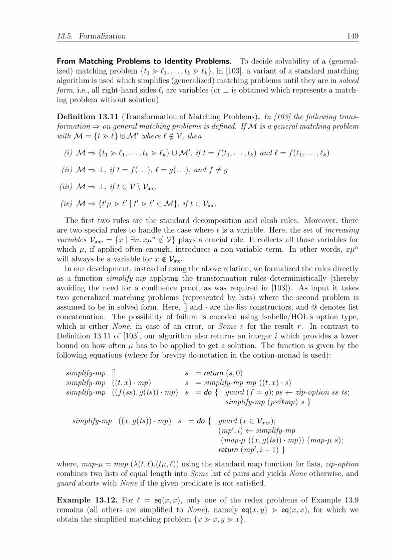
13.5. Formalization 149
From Matching Problems to Identity Problems. To decide solvability of a (general-ized) matching problem {t1 m `1, . . . , tk m `k}, in [103], a variant of a standard matchingalgorithm is used which simplifies (generalized) matching problems until they are in solvedform, i.e., all right-hand sides `i are variables (or ⊥ is obtained which represents a match-ing problem without solution).
Definition 13.11 (Transformation of Matching Problems). In [103] the following trans-formation⇒ on general matching problems is defined. IfM is a general matching problemwith M = {t m `} ]M′ where ` /∈ V, then
(i) M⇒ {t1 m `1, . . . , tk m `k} ∪M′, if t = f(t1, . . . , tk) and ` = f(`1, . . . , `k)
(ii) M⇒⊥, if t = f(. . .), ` = g(. . .), and f 6= g
(iii) M⇒⊥, if t ∈ V \ Vincr
(iv) M⇒ {t′µ m `′ | t′ m `′ ∈M}, if t ∈ Vincr
The first two rules are the standard decomposition and clash rules. Moreover, thereare two special rules to handle the case where t is a variable. Here, the set of increasingvariables Vincr = {x | ∃n. xµn /∈ V} plays a crucial role. It collects all those variables forwhich µ, if applied often enough, introduces a non-variable term. In other words, xµn
will always be a variable for x /∈ Vincr.In our development, instead of using the above relation, we formalized the rules directly
as a function simplify-mp applying the transformation rules deterministically (therebyavoiding the need for a confluence proof, as was required in [103]). As input it takestwo generalized matching problems (represented by lists) where the second problem isassumed to be in solved form. Here, [] and · are the list constructors, and @ denotes listconcatenation. The possibility of failure is encoded using Isabelle/HOL’s option type,which is either None, in case of an error, or Some r for the result r. In contrast toDefinition 13.11 of [103], our algorithm also returns an integer i which provides a lowerbound on how often µ has to be applied to get a solution. The function is given by thefollowing equations (where for brevity do-notation in the option-monad is used):
simplify-mp [] s = return (s, 0)simplify-mp ((t, x) ·mp) s = simplify-mp mp ((t, x) · s)simplify-mp ((f(ss), g(ts)) ·mp) s = do { guard (f = g); ps ← zip-option ss ts ;
simplify-mp (ps@mp) s }
simplify-mp ((x, g(ts)) ·mp) s = do { guard (x ∈ Vincr);(mp ′, i)← simplify-mp(map-µ ((x, g(ts)) ·mp)) (map-µ s);return (mp ′, i+ 1) }
where, map-µ = map (λ(t, `).(tµ, `)) using the standard map function for lists, zip-optioncombines two lists of equal length into Some list of pairs and yields None otherwise, andguard aborts with None if the given predicate is not satisfied.
Example 13.12. For ` = eq(x, x), only one of the redex problems of Example 13.9remains (all others are simplified to None), namely eq(x, y) m eq(x, x), for which weobtain the simplified matching problem {x m x, y m x}.

150 Chapter 13. Certification of Nontermination Proofs
In our formalization we show all relevant properties of simplify-mp, i.e., termination,preservation of solvability, and that simplify-mp mp [], if successful, is in solved form.Moreover, we prove the computed lower bound to be sound.
Theorem 13.13. The function simplify-mp satisfies the following properties:
• It is terminating.
• It is complete, i.e., if (n, σ) is a solution for mp then there are mp ′ and i such thatsimplify-mp mp [] = Some (mp ′, i), i 6 n, and (n− i, σ) is a solution for mp ′;
• It is sound, i.e., if (n, σ) is a solution for mp ′ and simplify-mp mp [] = Some (mp ′, i)then (n+ i, σ) is a solution for mp;
• If simplify-mp mp [] = Some (mp ′, i) then mp ′ is in solved form.
Proof. For termination of simplify-mp mp s , where mp = [(t1, `1), . . . , (tk, `k)], we use thelexicographic combination of the following two measures: first, we measure the sum of thesizes of the `i; and second, we measure the sum of the distances of the ti before turninginto non-variables. Here, the distance of some term ti before turning into a non-variableis 0 if ti ∈ V \ Vincr and the least number d such that tiµ
d /∈ V , otherwise.For this lexicographic measure, we get a decrease in the first component for the first and
the second recursive call, and a decrease in the second component for the third recursivecall.
Proving soundness and completeness is done via the following property which is provenby induction on the call structure of simplify-mp.
Whenever simplify-mp mp s = r then
• if r = None then mp ∪ s is not solvable,
• if r = Some (mp ′, i), there is no solution (n, σ) for mp ∪ s where n < i, and (n, σ)is a solution for mp ′ iff (n+ i, σ) is a solution for mp ∪ s .
Finally, the fact that simplify-mp mp [] is in solved form is shown by an easy induc-tion proof on the call structure of simplify-mp, where [] is generalized to an arbitrarygeneralized matching problem that is in solved form.
Although simplify-mp is defined as a recursive function, it cannot directly be used as acertification algorithm, due to the following two problems:
The first problem is that Vincr is not executable, since it contains an existential statement(remember that we had a similar problem for W earlier). Again, Vincr could be computedvia a fixpoint computation accompanied by a tedious manual termination proof. Instead,we once more employ reflexive transitive closures to characterize Vincr, which allows us touse the algorithm of [98] to compute it.
Lemma 13.14. Let R = {(x, y) | x 6= y, x = yµ, x ∈ V , y ∈ V}. Then Vincr = {y | ∃x ∈V , xµ /∈ V , (x, y) ∈ R∗}.
The second problem is the usage of implicit parameters. Recall that at the end ofSect. 13.4 we just fixed some substitution µ (which corresponds to what we did in our for-malization using Isabelle/HOL’s locale mechanism). Obviously, both Vincr and simplify-mp

13.5. Formalization 151
depend on µ. Hence, we have to pass µ as argument to both. As a result, the modifiedversion of the last equation of simplify-mp looks as follows:
simplify-mp µ ((x, g(ts)) ·mp) s = do {guard (x ∈ Vincr(µ));(mp ′, i)← simplify-mp µ (map-µ ((x, g(ts)) ·mp)) (map-µ s);return (mp ′, i+ 1) }
(7)
The problem of equation (7) is its inefficiency: In every recursive call, the set of increasingvariables Vincr(µ) is newly computed. Therefore, the obvious idea is to compute Vincr(µ)once and for all and pass it as an additional argument V .
simplify-mp µ V ((x, g(ts)) ·mp) s = do {guard (x ∈ V );(mp ′, i)← simplify-mp µ V (map-µ ((x, g(ts)) ·mp)) (map-µ s);return (mp ′, i+ 1) }
(8)
This version does not have the problem of recomputing Vincr(µ) and we just have to replacethe initial call simplify-mp µ mp [] by simplify-mp µ Vincr(µ) mp [].
Although, this looks straightforward and maybe not even worth mentioning, we stressthat this solution does not work properly. The problem is that by introducing V ,we can call simplify-mp using some V 6= Vincr(µ), which can cause nontermination.Take for example µ as the empty substitution and V = {x}, then the function callsimplify-mp µ V [(x, g(ts))] [] directly leads to exactly the same function call via (8).Hence, termination of simplify-mp defined by (8) cannot be proven. Therefore, the func-tion package of Isabelle/HOL [69] weakens equality (8) by the assumption that simplify-mphas to be terminating on the arguments µ, V , ((x, g(ts)) ·mp), and s .
Of course, we can instantiate (8) by V = Vincr(µ). Then we can get rid of the additionalassumption. But still, the corresponding unconditional equation is not suitable for codegeneration, since Vincr on the left-hand side is not a constructor.
Our final solution is to use the recent partial-function [70] command of Isabelle/HOLwhich generates unconditional equations even for nonterminating functions, provided thatsome syntactic restrictions are met (only one defining equation and the function musteither return an option type or be tail-recursive).
Since simplify-mp already returns an option type, we just had to merge all equationsinto a single case statement. (If the result is not of option type, we can just wrap theoriginal return type into an option type). Afterwards the partial-function command isapplicable and we obtain an equation similar to (8) which can be processed by the codegenerator and efficiently computes simplify-mp without recomputing Vincr(µ). Moreover,since we have already shown termination of the inefficient version of simplify-mp, we knowthat also the efficient version does terminate whenever it is called with V = Vincr(µ). Inour formalization we actually have two versions of simplify-mp: an abstract version whichis unsuitable for code generation (and also inefficient) and a concrete version. All theabove properties are proven on the abstract version neglecting any efficiency problems.Afterwards it is shown that the concrete version computes the same results as the abstractone (which is relatively easy since the call-structure is the same). In this way, we get thebest of two worlds: abstraction and ease of reasoning from the abstract version (using sets,existential statements, and the induction rules from the function package), and efficiencyfrom the concrete version (using lists and concrete functions to obtain witnesses).
The above mentioned problem is not restricted to simplify-mp. Whenever the termi-nation of a function relies on the correct initialization of some precomputed values, asimilar problem arises. Currently, this can be solved by writing a second function via the

152 Chapter 13. Certification of Nontermination Proofs
partial-function command, as shown above. Although the second definition is mainly acopy of the original one, we can currently not recommend to use it as a replacement, sincethe function package provides much more convenience for standard definitions than whenusing the partial-function command. If the functionality of partial functions is extended,the situation might change (and we would welcome any effort in that direction).
Continuing with deciding matching problems, we are in the situation, that by usingsimplify-mp we can either directly detect that a matching problem is unsolvable or obtainan equivalent generalized matching problem in solved form M = {t1 m x1, . . . , tk m xk}.In principle, M has the solution (n, σ) where n is arbitrary and σ(xi) = tiµ
n. However,this definition of σ is not always well-defined if there are i and j such that xi = xj andi 6= j. To decide whether it is possible to adapt the proposed solution, we must knowwhether tiµ
n = tjµn for some n, i.e., we must solve the identify problem ti u tj.
The following result of [103, Theorem 14 (iv)] is easily formalized and also poses nochallenges for certification. Afterwards it remains to decide identity problems.
Theorem 13.15. Let M = {t1 m x1, . . . , tk m xk} be a generalized matching problem insolved form. Define Iinit = {ti u tj | 1 6 i < j 6 k, xi = xj}. Then M is solvable iff allidentity problems in Iinit are solvable.
To prove this theorem, the key observation is that we can always combine severalsolutions of identity problems: Whenever nij are solutions to the identity problems ti u tj,respectively, then the maximum n of all nij is a solution to all identity problems ti u tj.And then also (n, σ) is a solution to M where σ(xi) = tiµ
n is guaranteed to be well-defined.
Example 13.16. For the remaining matching problem of Example 13.12 we generate oneidentity problem: x u y.
Deciding Identity Problems. In [103, Section 3.4] a complicated algorithm is presentedto decide solvability of an identity problem s u t. The main idea is to iteratively generate(s, t), (sµ, tµ), (sµ2, tµ2), . . . until either some (sµi, tµi) with sµi = tµi is generated,or it can be detected that no solution exists. For the latter, some easy conditions forunsolvability are identified, e.g., sµi = C[f(ss)] and tµi = C[x] where x /∈ Vincr. However,these conditions do not suffice to detect all unsolvable identity problems. Therefore, ineach iteration conflicts (indicating which subterms have to become equal after applyingµ several times, to obtain overall equality), are stored in a set S, and two sufficientconditions on pairs of conflicts from S are presented that allow to conclude unsolvability.
For the overall algorithm, soundness is rather easy to establish, completeness is morechallenging, and the termination proof is the most difficult part. To be more precise, itis shown that nontermination of the algorithm allows to construct an infinite sequenceof terms where no two terms are embedded into each other (which is not possible dueto Kruskal’s tree theorem). Hence, the formalization would require a formalization ofthe tree theorem. Moreover, the implicit complexity bound on the number of requirediterations is quite high.
The reason for using Kruskal’s tree theorem is that in [103] the conflicts in S consist ofa variable, a position, and a term which is not bounded in its size. So, there is no a prioribound on S. We were able to simplify the decision procedure for s u t considerably sincewe only store conflicts whose constituting terms are in the set of conflict terms
CT (s, t) = {u | v D u, v ∈ {s, t} ∪ ran(µ)}.

13.5. Formalization 153
To be more precise, all conflicts are of the form (u, v,m) where (u, v) is contained in thefinite set S = (CT (s, t)∩V)×CT (s, t). Whenever we see a conflict (u, v, ) for the secondtime, the algorithm stops. Thus, we get a decision procedure which needs at most |S|iterations and whose termination proof is easy. In contrast to [103], our procedure doesneither require any preprocessing on µ nor unification.
The key idea to get an a priory bound on the set of conflicts, is to consider identityproblems of a generalized form s u tµn which can be represented by the triple (s, t, n).Then applying substitutions can be done by increasing n, and all terms that are generatedduring an execution of the algorithm are terms from CT (s, t).
Before presenting the main algorithm for deciding identity problems s u tµn, we requirean auxiliary algorithm conflicts (s, t, n) that computes the set of conflicts for an identityproblem, i.e., subterms of s and tµn with different roots.
conflicts (s, y, n+ 1) = conflicts (s, µ(y), n)conflicts (x, y, 0) = if x = y then ∅ else {(x, y, 0)}conflicts (f(ss), y, 0) = {(y, f(ss), 0)}conflicts (x, g(ts), n) = {(x, g(ts), n)}conflicts (f(ss), g(ts), n) = if f = g ∧ |ss| = |ts|
then⋃
(si,ti)∈zip ss ts conflicts (si, ti, n)
else {(f(ss), g(ts), n)}
We identified and formalized the following properties of conflicts and CT .
Lemma 13.17. • sσ = tµnσ iff ∀(u, v,m) ∈ conflicts (s, t, n). uσ = vµmσ.
• if (u, v,m) ∈ conflicts (s, t, n) then
– root(u) 6= root(v)
– v ∈ V implies m = 0 ∧ u ∈ V– ∃k p. n = m+ k ∧ ((s|p, tµk|p) = (u, v) ∨ ((s|p, tµk|p) = (v, u) ∧m = 0))
– {u, v} ⊆ CT (s, t)
• {u, v} ⊆ CT (s, t) implies CT (u, v) ⊆ CT (s, t)
• CT (u, v) ⊆ CT (uµ, v) whenever u ∈ V
Using conflicts we can now formulate the algorithm ident-solve which decides identityproblem s u t if invoked with ident-solve ∅ (s, t, 0).
ident-solve S idp =let C = conflicts idp inif (f(us), , ) ∈ C ∨ ((u, v, ) ∈ C ∧ (u, v, ) ∈ S) then None else do {
ns ← map-option (λ(u, v,m). ident-solve ({(u, v,m)} ∪ S) (uµ, v,m+ 1)) C;return (max {n+ 1 | n ∈ ns}) }
where map-option is a variant of the map function on lists whose overall result is None ifthe supplied function returns None for any element of the given list.
Example 13.18. We continue Example 13.16 by invoking ident-solve ∅ (x, y, 0). Thisleads to the conflict (x, y, 0). Afterwards, ident-solve {(x, y, 0)} (cons(z, y), y, 1) is invokedwhich results in the conflict (y, x, 0). Finally, the conflict (x, y, 0) is generated again whencalling ident-solve {(x, y, 0), (y, x, 0)} (cons(z, x), x, 1) and the result None is obtained.

154 Chapter 13. Certification of Nontermination Proofs
We formalized termination, soundness, and completeness of ident-solve.
Lemma 13.19 (Termination). ident-solve is terminating.
Proof. Take the measure function λS (s , t , ). |(CT (s, t)∩V)×CT (s, t)\{(a, b) | (a, b, ) ∈S}|. Then the actual termination proof boils down to showing
L := (CT (s, t) ∩ V)× CT (s, t) \ {(a, b) | (a, b, ) ∈ S}⊃ (CT (uµ, v) ∩ V)× CT (uµ, v) \ {(a, b) | (a, b, ) ∈ {(u, v,m)} ∪ S} =: R
whenever ident-solve S (s, t, n) leads to a call ident-solve ({(u, v,m)} ∪ S) (uµ, v,m+ 1),i.e., whenever (u, v,m) ∈ conflicts (s, t, n), (u, v, ) /∈ S, and u ∈ V . By Lemma 13.17 weobtain {u, v} ⊆ CT (s, t) and CT (uµ, v) ⊆ CT (u, v) ⊆ CT (s, t). Hence, L ⊇ R and since(u, v) ∈ L \R we even have L ⊃ R.
Lemma 13.20 (Soundness). If ident-solve S (s, t, n) = Some i then sµi = tµnµi.
Proof. We perform induction on the call-structure of ident-solve. So, assume ident-solve S(s, t, n) = Some i. By definition of ident-solve, for all (u, v,m) ∈ conflicts (s, t, n) thereis some j such that ident-solve ({(u, v,m)} ∪ S) (uµ, v,m + 1) = Some j and i is themaximum of all j + 1. Using the induction hypothesis, we conclude uµj+1 = uµµj =vµm+1µj = vµmµj+1 for all (u, v,m) ∈ conflicts (s, t, n), and since i ≥ j + 1 we alsoachieve uµi = vµmµi. But this is equivalent to sµi = tµnµi by Lemma 13.17 (whereσ = µi).
Lemma 13.21 (Completeness). Whenever the identity problem s u t is solvable thenident-solve ∅ (s, t, 0) 6= None.
Proof. If s u t is solvable then there is some N such that sµN = tµN . Our actualproof shows the following property (?) for all S, s′, t′, n, n′, and p where (a, b)
↔= (c, d)
abbreviates (a, b) = (c, d) ∨ (a, b) = (d, c).1
(sµn|p, tµn|p)↔= (s′, t′µn
′) (9)
−→ (∀(u, v,m) ∈ S. (m = 0 ∨ v /∈ V) ∧ root(u) 6= root(v) ∧ (10)
(∃q1 q2 n1. p = q1q2 ∧ n1 < n ∧ (sµn1|q1 , tµn1|q1)↔= (u, vµm)))
−→ ident-solve S (s′, t′, n′) 6= None (11)
Once (?) is established, the lemma immediately follows from (?) which is instantiated byS = ∅, s′ = s, t′ = t, n′ = n = 0, and p = ε (the empty position).
To prove (?), we perform induction on the call-structure of ident-solve. So, we assume(9) and (10), and have to show (11). By sµN = tµN we conclude sµn|pµN = sµNµn|p =tµNµn|p = tµn|pµN , and thus s′µN = t′µn
′µN by (9). By Lemma 13.17 this shows uµN =
vµmµN for all (u, v,m) ∈ conflicts (s′, t′, n′) =: C. In a similar way we prove uµN = vµmµN
for all (u, v,m) ∈ S using (10).Next we consider an arbitrary (u, v,m) ∈ C. By Lemma 13.17 we have root(u) 6=
root(v), m = 0∨ v /∈ V , and there are q1 and k such that n′ = m+ k and (s′|q1 , t′µk|q1) =(u, v) ∨ ((s′|q1 , t′µk|q1) = (v, u) ∧ m = 0). In particular, this implies (s′|q1 , t′µk|q1µm)
↔=
(u, vµm). Moreover, we know uµN = vµmµN .
1In the formalization, (?) looks even more complicated, since here we dropped all parts that restrict pand q1 to valid positions.

13.5. Formalization 155
First, we show that u ∈ V , and hence the condition (f(us), , ) ∈ C is not satisfied. Thereason is that u /∈ V also implies v /∈ V by Lemma 13.17 which implies the contradictionroot(u) = root(uµN) = root(vµmµN) = root(v) 6= root(u).
Second, ident-solve ({(u, v,m)}∪S) (uµ, v,m+1) 6= None. To show this, we just applythe induction hypothesis where it remains to show that (9) and (10) are satisfied (wherethe values of S, s′ ,t′ ,n, n′, p are {(u, v,m)}∪S, uµ, v, n+1, m+1, and pq1, respectively).To this end, we derive the following equality.
(sµn|pq1 , tµn|pq1) = (sµn|p|q1 , tµn|p|q1)↔= (s′|q1 , t′µn
′ |q1)= (s′|q1 , t′µk|q1µm)
↔= (u, vµm).
(12)
Using (12), root(u) 6= root(v), and m = 0 ∨ v /∈ V , we conclude that (10) is satisfied forthe new conflict (u, v,m). Moreover, (10) is trivially satisfied for all (old) conflicts in S,by using (10) (for the old inputs (s′, t′, n′), . . .). Finally, by applying µ on all terms in(12) we obtain (sµn+1|pq1 , tµn+1|pq1)
↔= (uµ, vµm+1) which is exactly the required (9).
The last potential reason for ident-solve S (s′, t′, n′) to be None, is that there is somem′ such that (u, v,m′) ∈ S. We assume that such an m′ exists and eventually show acontradiction (the most difficult part of this proof). By (10) we conclude that m′ = 0∨v /∈V and there are p1, q3, and n2 where p = p1q3, n2 < n, and (sµn2|p1 , tµn2 |p1)
↔= (u, vµm
′).
Since n2 < n there is some k1 with n = n2 + k1 and k1 > 0. Starting from (12) we derive
(u, vµm)↔= (sµn|pq1 , tµn|pq1)
= (sµn2+k1 |p1q3q1 , tµn2+k1 |p1q3q1) = (sµn2|p1σ|q, tµn2|p1σ|q)↔= (uσ|q, vµm
′σ|q)
(13)
where σ and q are abbreviations for µk1 and q3q1, respectively. Using (13) it is possibleto derive a contradiction via a case analysis.
If m′ = m then (13) yields both uσσ|qq = u and vµmσσ|qq = vµm. Thus, u(σσ)i|(qq)i = uand vµm(σσ)i|(qq)i = vµm for all i. For m′ = m we can further show u 6= vµm and hence,u(σσ)i|(qq)i 6= vµm(σσ)i|(qq)i for all i. This leads to the desired contradiction since we knowthat uµN = vµmµN , and hence u(σσ)N = uµ2k1N = uµNµ(2k1−1)N = vµmµNµ(2k1−1)N =vµmµ2k1N = vµm(σσ)N , which shows that for i = N the previous inequality does nothold.
Otherwise m 6= m′. Hence, m 6= 0 ∨m′ 6= 0 and in combination with m = 0 ∨ v /∈ Vand m′ = 0 ∨ v /∈ V we conclude v /∈ V . Thus, u ∈ V by Lemma 13.17 as (u, v,m) ∈conflicts (s′, t′, n′). Then by a case analysis on (13) we can show that there are i andj such that uµi B uµj. Moreover, from uµN = vµmµN and uµN = vµm
′µN we obtain
uµN+m = uµN+m′ . In combination with m 6= m′ and uµi B uµj this leads to the desiredcontradiction.
Putting all lemmas on ident-solve together, we can even give a decision procedure foridentity problems which does not require ident-solve at all, and shows an explicit boundon a solution.
Theorem 13.22. An identity problem s u t is solvable iff sµn = tµn where n = |CT (s, t)∩V| · |CT (s, t)|.
Proof. If an identity problem is solvable, then the result of ident-solve ∅ (s, t, 0) = Some ifor some i by Lemma 13.21. From the termination proof in Lemma 13.19 we know thati 6 |CT (s, t)∩V|·|CT (s, t)| = n (unfortunately, in Isabelle/HOL we could not extract thisknowledge from the termination proof and had to formalize this simple result separately).And by Lemma 13.20 we infer that sµi = tµi. But then also sµn = tµn.

156 Chapter 13. Certification of Nontermination Proofs
Note that |CT (s, t)| 6 |s| + |t| + |µ| where |µ| is the size of all terms in the rangeof µ. Hence, the value of n in Theorem 13.22 is quadratic in the size of the inputproblem. We conjecture that even a linear bound exists, although some proof attemptsfailed. As an example, we tried to replace the condition (u, v, ) ∈ C ∧ (u, v, ) ∈ S by(u, , ) ∈ C ∧ (u, , ) ∈ S in ident-solve to get a linear number of iterations. However,then ident-solve is not complete anymore.
13.6. Conclusions
We have formalized several techniques to certify compositional (innermost) nontermina-tion proofs, where the hardest part was the decision procedure of [103], which decideswhether a loop is an innermost loop. In our formalization, we were able to simplify thealgorithm and the proofs for identity problems considerably: a complex algorithm can bereplaced by a single line due to Theorem 13.22.
With this result we can also show (but have not formalized) that all considered decisionproblems of this paper are in P.
Theorem 13.23. Deciding whether an identity problem, a matching problem, or a redexproblem is solvable is in P. Moreover, deciding whether a loop is an innermost loop is inP.
Proof. We start with identity problems. By Theorem 13.22 we just have to check sµn =tµn for n = |CT (s, t)∩V|·|CT (s, t)|. When using DAG compressed terms we can representsµn and tµn in polynomial space and in turn use the algorithms of [19,91] to check equalityin polynomial time. Note that even if the input (s, t, µ) is already DAG compressed, theproblem is still in P. The reason is that |CT (s, t)| 6 |s|+ |t|+ |µ| also holds when sizes ofterms are measured according to their DAG representation.
For matching problems t m `, we first observe that simplify-mp [(t, `)] [] requires at most|Vincr| · |`| many iterations, and when using DAG compression, the resulting simplifiedmatching problem can be represented in polynomial space. Hence, the resulting identityproblems can all be solved in polynomial time.
Using the result for matching problems, by Theorem 13.8 it follows that redex problemst |m ` are decidable in P: The number of matching problems in Minit as well as the sizeof each element of Minit is linear in the sizes of t, `, and µ.
Finally, since redex problems can be decided in P, by Lemma 13.5 this also holds forthe question, whether a loop is an innermost loop.
We have also shown how reflexive transitive closures can be used to avoid terminationproofs, and how partial functions help to develop efficient algorithms.
We tested our algorithms within our certifier CeTA (version 2.3) in combination with thetermination analyzer AProVE [39], which is (as far as we know) currently the only tool, thatcan prove innermost nontermination of term rewrite systems. Through our experiments,a major soundness bug in AProVE was revealed: one of the two loop-finding methodscompletely ignored the strategy. After this bug was fixed, all generated nonterminationproofs could be certified. Since the overhead for certification is negligible (AProVE required151 minutes to generate all proofs, whereas CeTA required 4 seconds to certify them),we encourage termination tool users to always certify their proofs. For more detailson the experiments, we refer to http://cl-informatik.uibk.ac.at/software/ceta/
experiments/nonterm/.

13.6. Conclusions 157
Future work consists of integrating further techniques for which completeness is notobvious into our framework. Examples are innermost narrowing [3] and the switch frominnermost termination to termination for TRSs and DPPs.
Acknowledgments
We thank Lukas Bulwahn for helpful information on Isabelle/HOL’s predicate compiler.


Bibliography
[1] E. Albert, P. Arenas, S. Genaim, M. Gomez-Zamalloa, G. Puebla, D. V. Ramırez-Deantes, G. Roman, and D. Zanardini. Termination and cost analysis with COSTAand its user interfaces. ENTCS, 258(1):109–121, 2009.
[2] T. Aoto, T. Yoshida, and J. Toyama. Proving confluence of term rewriting systemsautomatically. In Proc. of the 20th International Conference on Rewriting Tech-niques and Applications (RTA 2009), volume 5595 of LNCS, pages 93–102, 2009.
[3] T. Arts and J. Giesl. Termination of term rewriting using dependency pairs. Theor.Comput. Sci., 236(1-2):133–178, 2000.
[4] M. Avanzini, G. Moser, and A. Schnabl. Automated implicit computational com-plexity analysis (system description). In Proc. of the 4th International Joint Confer-ence on Automated Reasoning (IJCAR 2008), volume 5195 of LNAI, pages 132–138,2008.
[5] F. Baader and T. Nipkow. Term Rewriting and All That. Cambridge UniversityPress, 1998.
[6] G. Barthe, J. Forest, D. Pichardie, and V. Rusu. Defining and reasoning aboutrecursive functions: a practical tool for the Coq proof assistant. In Proc. of the 8thInternational Symposium on Functional and Logic Programming (FLOPS 2006),volume 3945 of LNCS, pages 114–129, 2006.
[7] A. M. Ben-Amram and M. Codish. A SAT-based approach to size change termina-tion with global ranking functions. In Proc. of the 16th International Conference onTools and Algorithms for the Construction and Analysis of Systems (TACAS 2008),volume 4963 of LNCS, pages 218–232, 2008.
[8] A. M. Ben-Amram and C. S. Lee. Program termination analysis in polynomial time.ACM Trans. Program. Lang. Syst., 29(1), 2007.
[9] A. Ben Cherifa and P. Lescanne. Termination of rewriting systems by polynomial in-terpretations and its implementation. Science of Computer Programming, 9(2):137–159, 1987.
[10] S. Berghofer, L. Bulwahn, and F. Haftmann. Turning inductive into equationalspecifications. In Proc. of the 22nd International Conference on Theorem Provingin Higher Order Logics (TPHOLs 2009), volume 5674 of LNCS, pages 131–146,2009.
[11] Y. Bertot and P. Casteran. Interactive Theorem Proving and Program Development;Coq’Art: The Calculus of Inductive Constructions. TCS Texts. Springer, 2004.

160 Bibliography
[12] F. Blanqui, W. Delobel, S. Coupet-Grimal, S. Hinderer, and A. Koprowski. CoLoR, aCoq library on rewriting and termination. In Proc. of the 8th International Workshopon Termination (WST 2006), pages 69–73, 2006.
[13] F. Blanqui and A. Koprowski. CoLoR: a Coq library on well-founded rewrite rela-tions and its application to the automated verification of termination certificates.Mathematical Structures in Computer Science, 21(4):827–859, 2011.
[14] R. S. Boyer and J. S. Moore. A Computational Logic. Academic Press, 1980.
[15] M. Brockschmidt, R. Musiol, C. Otto, and J. Giesl. Automated termination proofsfor Java programs with cyclic data. In Proc. of the 24th International Conferenceon Computer Aided Verification (CAV 2012), volume 7358 of LNCS, pages 105–122,2012.
[16] M. Brockschmidt, C. Otto, C. von Essen, and J. Giesl. Termination graphs forJava bytecode. In Verification, Induction, Termination Analysis - Festschrift forChristoph Walther on the Occasion of His 60th Birthday, volume 6463 of LNCS,pages 17–37, 2010.
[17] W. Buchholz. Proof-theoretic analysis of termination proofs. Ann. Pure Appl. Logic,75(1-2):57–65, 1995.
[18] L. Bulwahn, A. Krauss, and T. Nipkow. Finding lexicographic orders for terminationproofs in Isabelle/HOL. In Proc. of the 20th International Conference on TheoremProving in Higher Order Logics (TPHOLs 2007), volume 4732 of LNCS, pages 38–53, 2007.
[19] G. Busatto, M. Lohrey, and S. Maneth. Efficient memory representation of XMLdocuments. In Proc. of the 10th International Symposium on Database ProgrammingLanguages (DBPL 2005), volume 3774 of LNCS, pages 199–216, 2005.
[20] M. Codish, C. Fuhs, J. Giesl, and P. Schneider-Kamp. Lazy abstraction for size-change termination. In Proc. of the 17th International Conference on Logic forProgramming, Artificial Intelligence and Reasoning (LPAR 2010), volume 6397 ofLNCS, pages 217–232, 2010.
[21] E. Contejean, P. Courtieu, J. Forest, O. Pons, and X. Urbain. Certification ofautomated termination proofs. In Proc. of the 6th International Symposium onFrontiers of Combining Systems (FroCoS 2007), volume 4720 of LNAI, pages 148–162, 2007.
[22] E. Contejean, C. Marche, B. Monate, and X. Urbain. CiME. http://cime.lri.fr.
[23] E. Contejean, A. Paskevich, X. Urbain, P. Courtieu, O. Pons, and J. Forest. A3PAT,an approach for certified automated termination proofs. In Proc. of the ACM SIG-PLAN Workshop on Partial Evaluation and Program Manipulation (PEPM 2010),pages 63–72, 2010.
[24] B. Cook, A. Podelski, and A. Rybalchenko. Termination proofs for systems code.In Proc. of the ACM SIGPLAN Conference on Programming Language Design andImplementation (PLDI 2006), pages 415–426, 2006.

Bibliography 161
[25] P. Courtieu, J. Forest, and X. Urbain. Certifying a termination criterion based ongraphs, without graphs. In Proc. of the 21st International Conference on TheoremProving in Higher Order Logics (TPHOLs 2008), volume 5170 of LNCS, pages 183–198, 2008.
[26] N. Dershowitz. Orderings for term-rewriting systems. Theor. Comput. Sci., 17:279–301, 1982.
[27] N. Dershowitz. Termination of rewriting. J. Symb. Comp., 3(1-2):69–116, 1987.
[28] N. Dershowitz. Termination dependencies. In Proc. of the 6th International Work-shop on Termination (WST 2003), pages 27–30, 2003.
[29] N. Dershowitz and Z. Manna. Proving termination with multiset orderings. Comm.of the ACM, 22(8):465–476, 1979.
[30] F. Emmes, T. Enger, and J. Giesl. Proving non-looping non-termination automat-ically. In Proc. of the 6th International Joint Conference on Automated Reasoning(IJCAR 2012), volume 7364 of LNAI, pages 225–240, 2012.
[31] J. Endrullis. Jambox. Available from http://joerg.endrullis.de.
[32] J. Endrullis, J. Waldmann, and H. Zantema. Matrix interpretations for provingtermination of term rewriting. Journal of Automated Reasoning, 40(2-3):195–220,2008.
[33] C. Fuhs, J. Giesl, A. Middeldorp, P. Schneider-Kamp, R. Thiemann, and H. Zankl.Maximal termination. In Proc. of the 19th International Conference on RewritingTechniques and Applications (RTA 2008), volume 5117 of LNCS, pages 110–125,2008.
[34] A. L. Galdino and M. Ayala-Rincon. A PVS theory for term rewriting systems.ENTCS, 247:67–83, 2009.
[35] A. L. Galdino and M. Ayala-Rincon. A formalization of the Knuth-Bendix(-Huet)critical pair theorem. Journal of Automated Reasoning, 45(3):301–325, 2010.
[36] A. Geser, D. Hofbauer, J. Waldmann, and H. Zantema. On tree automata thatcertify termination of left-linear term rewriting systems. Information and Compu-tation, 205(4):512–534, 2007.
[37] J. Giesl and T. Arts. Verification of Erlang processes by dependency pairs. Appl.Alg. Eng. Comm. Comput., 12(1,2):39–72, 2001.
[38] J. Giesl, M. Raffelsieper, P. Schneider-Kamp, S. Swiderski, and R. Thiemann. Au-tomated termination proofs for Haskell by term rewriting. ACM Transactions onProgramming Languages and Systems, 33(2):7:1–7:39, 2011.
[39] J. Giesl, P. Schneider-Kamp, and R. Thiemann. AProVE 1.2: Automatic terminationproofs in the dependency pair framework. In Proc. of the 3rd International JointConference on Automated Reasoning (IJCAR 2006), volume 4130 of LNAI, pages281–286, 2006.

162 Bibliography
[40] J. Giesl, R. Thiemann, and P. Schneider-Kamp. The dependency pair framework:Combining techniques for automated termination proofs. In Proc. of the 11th Inter-national Conference on Logic for Programming, Artificial Intelligence and Reasoning(LPAR 2004), volume 3452 of LNAI, pages 301–331, 2005.
[41] J. Giesl, R. Thiemann, and P. Schneider-Kamp. Proving and disproving terminationof higher-order functions. In Proc. of the 5th International Symposium on Frontiersof Combining Systems (FroCoS 2005), volume 3717 of LNAI, pages 216–231, 2005.
[42] J. Giesl, R. Thiemann, P. Schneider-Kamp, and S. Falke. Mechanizing and improv-ing dependency pairs. Journal of Automated Reasoning, 37(3):155–203, 2006.
[43] M. Gordon. From LCF to HOL: a short history. In Proof, Language, and Interaction,Essays In Honour of Robin Milner, pages 169–186. MIT Press, 2000.
[44] M. Gordon. From LCF to HOL: A short history. In Proof, Language, and Interac-tion, pages 169–185. MIT Press, 2000.
[45] M. J. C. Gordon, R. Milner, and C. P. Wadsworth. Edinburgh LCF, volume 78 ofLNCS. Springer, 1979.
[46] B. Gramlich. Abstract relations between restricted termination and confluence prop-erties of rewrite systems. Fundamenta Informaticae, 24:3–23, 1995.
[47] S. Gulwani, K. Mehra, and T. Chilimbi. SPEED: precise and efficient static estima-tion of program computational complexity. In Proc. of the 36th ACM Symposiumon Principles of Programming Languages (POPL 2009), pages 127–139, 2009.
[48] F. Haftmann. Code generation from Isabelle/HOL theories, Apr. 2009. http://
isabelle.in.tum.de/doc/codegen.pdf.
[49] F. Haftmann and T. Nipkow. Code generation via higher-order rewrite systems. InProc. of the 10th International Symposium on Functional and Logic Programming(FLOPS 2010), volume 6009 of LNCS, pages 103–117, 2010.
[50] N. Hirokawa and A. Middeldorp. Automating the dependency pair method. Infor-mation and Computation, 199(1-2):172–199, 2005.
[51] N. Hirokawa and A. Middeldorp. Tyrolean Termination Tool: Techniques and fea-tures. Information and Computation, 205(4):474–511, 2007.
[52] N. Hirokawa and A. Middeldorp. Decreasing diagrams and relative termination.Journal of Automated Reasoning, 47(4):481–501, 2011.
[53] N. Hirokawa, A. Middeldorp, and H. Zankl. Uncurrying for termination. In Proc. ofthe 15th International Conference on Logic for Programming, Artificial Intelligenceand Reasoning (LPAR 2008), volume 5330 of LNAI, pages 667–681, 2008.
[54] D. Hofbauer and J. Waldmann. Match-bounds for relative termination. In Proc. ofthe 11th International Workshop on Termination (WST 2010), 2010.
[55] J. Hoffmann, K. Aehlig, and M. Hofmann. Resource aware ML. In Proc. of the 24thInternational Conference on Computer Aided Verification (CAV 2012), volume 7358of LNCS, pages 781–786, 2012.

Bibliography 163
[56] H. Hong and D. Jakus. Testing positiveness of polynomials. Journal of AutomatedReasoning, 21(1):23–38, 1998.
[57] J.-P. Jouannaud and A. Rubio. The higher-order recursive path ordering. In Proc.of the 14.th Annual IEEE Symposium on Logic in Computer Science (LICS 1999),pages 402–411. IEEE Computer Society Press, 1999.
[58] S. Kamin and J. J. Levy. Two generalizations of the recursive path ordering. Un-published manuscript, University of Illinois, 1980.
[59] R. Kennaway, J. W. Klop, R. Sleep, and F.-J. de Vries. Comparing curried anduncurried rewriting. Journal of Symbolic Computation, 21(1):15–39, 1996.
[60] G. Klein, J. Andronick, K. Elphinstone, G. Heiser, D. Cock, P. Derrin, D. Elkaduwe,K. Engelhardt, R. Kolanski, M. Norrish, T. Sewell, H. Tuch, and S. Winwood. seL4:formal verification of an operating-system kernel. Comm. of the ACM, 53(6):107–115, 2010.
[61] G. Klein and T. Nipkow. A machine-checked model for a Java-like language, vir-tual machine, and compiler. ACM Transactions on Programming Languages andSystems, 28(4):619–695, 2006.
[62] A. Koprowski. TPA: Termination proved automatically. In Proc. of the 17th Inter-national Conference on Rewriting Techniques and Applications (RTA 2006), volume4098 of LNCS, pages 257–266, 2006.
[63] A. Koprowski. Coq formalization of the higher-order recursive path ordering. Appl.Alg. Eng. Comm. Comput., 20(5-6):379–425, 2009.
[64] A. Koprowski and J. Waldmann. Arctic termination . . . below zero. In Proc. ofthe 19th International Conference on Rewriting Techniques and Applications (RTA2008), volume 5117 of LNCS, pages 202–216, 2008.
[65] K. Korovin and A. Voronkov. Orienting rewrite rules with the Knuth-Bendix order.Information and Computation, 183(2):165–186, 2003.
[66] M. Korp and A. Middeldorp. Match-bounds revisited. Information and Computa-tion, 207(11):1259–1283, 2009.
[67] M. Korp, C. Sternagel, H. Zankl, and A. Middeldorp. Tyrolean Termination Tool 2.In Proc. of the 20th International Conference on Rewriting Techniques and Appli-cations (RTA 2009), volume 5595 of LNCS, pages 295–304, 2009.
[68] A. Krauss. Certified size-change termination. In Proc. of the 21st InternationalConference on Automated Deduction (CADE 2007), volume 4603 of LNCS, pages460–475, 2007.
[69] A. Krauss. Partial and nested recursive function definitions in higher-order logic.Journal of Automated Reasoning, 44(4):303–336, 2010.
[70] A. Krauss. Recursive definitions of monadic functions. In Proc. of the Workshop onPartiality and Recursion in Interactive Theorem Proving (PAR 2010), volume 43 ofEPTCS, pages 1–13, 2010.

164 Bibliography
[71] M. S. Krishnamoorthy and P. Narendran. On recursive path ordering. Theor.Comput. Sci., 40:323–328, 1985.
[72] J. B. Kruskal. Well-quasi-ordering, the tree theorem, and Vazsonyi’s conjecture.Transactions of the American Mathematical Society, 95(2):210–225, 1960.
[73] D. Lankford. On proving term rewrite systems are noetherian. Technical ReportMTP-3, Louisiana Technical University, Ruston, LA, USA, 1979.
[74] C. S. Lee, N. D. Jones, and A. M. Ben-Amram. The size-change principle forprogram termination. In Proc. of the 28th ACM Symposium on Principles of Pro-gramming Languages (POPL 2001), pages 81–92, 2001.
[75] A. Lochbihler. Verifying a compiler for Java threads. In Proc. of the 19th EuropeanSymposium on Programming (ESOP 2010), volume 6012 of LNCS, pages 427–447,2010.
[76] S. Lucas. Polynomials over the reals in proofs of termination: From theory topractice. RAIRO Theor. Inf. Appl., 39(3):547–586, 2005.
[77] M. Marchiori. Logic programs as term rewriting systems. In Proc. of the 4thInternational Conference on Algebraic and Logic Programming (ALP 1994), volume850 of LNCS, pages 223–241, 1994.
[78] A. Martelli and U. Montanari. An efficient unification algorithm. ACM Transactionson Programming Languages and Systems, 4(2):258–282, 1982.
[79] A. Middeldorp. Modular Properties of Term Rewriting Systems. PhD thesis, VrijeUniversiteit, Amsterdam, 1990.
[80] M. O. Myreen and J. Davis. A verified runtime for a verified theorem prover. InProc. of the 2nd International Conference on Interactive Theorem Proving (ITP2011), volume 6898 of LNCS, pages 265–280, 2011.
[81] F. Neurauter, H. Zankl, and A. Middeldorp. Revisiting matrix interpretations forpolynomial derivational complexity of term rewriting. In Proc. of the 17th Interna-tional Conference on Logic for Programming, Artificial Intelligence and Reasoning(LPAR 2010), volume 6397 of LNCS, pages 550–564, 2010.
[82] M. Nguyen, D. D. Schreye, J. Giesl, and P. Schneider-Kamp. Polytool: Polynomialinterpretations as a basis for termination analysis of logic programs. Theory andPractice of Logic Programming, 11(1):33–63, 2011.
[83] T. Nipkow. An inductive proof of the wellfoundedness of the multiset order, 1998.Available at http://www4.in.tum.de/~nipkow/misc/multiset.ps.
[84] T. Nipkow, L. C. Paulson, and M. Wenzel. Isabelle/HOL – A Proof Assistant forHigher-Order Logic, volume 2283 of LNCS. Springer, 2002.
[85] E. Ohlebusch. A simple proof of sufficient conditions for the termination of thedisjoint union of term rewriting systems. Bulletin of the EATCS, 50:223–228, 1993.
[86] E. Ohlebusch. Termination of logic programs: Transformational methods revisited.Appl. Alg. Eng. Comm. Comput., 12(1-2):73–116, 2001.

Bibliography 165
[87] C. Otto, M. Brockschmidt, C. von Essen, and J. Giesl. Automated terminationanalysis of Java bytecode by term rewriting. In Proc. of the 21st InternationalConference on Rewriting Techniques and Applications (RTA 2010), volume 6 ofLIPIcs, pages 259–276, 2010.
[88] S. Owre, J. M. Rushby, and N. Shankar. PVS: A prototype verification system. InProc. of the 11th International Conference on Automated Deduction (CADE 1992),volume 607 of LNAI, pages 748–752, 1992.
[89] L. C. Paulson. Logic and Computation: Interactive Proof with Cambridge LCF.Cambridge University Press, 1987.
[90] S. Peyton Jones et al. The Haskell 98 language and libraries: The revised report.Journal of Functional Programming, 13(1):0–255, Jan 2003.
[91] M. Schmidt-Schauß. Polynomial equality testing for terms with shared substruc-tures. Frank report 21, Institut fur Informatik. FB Informatik und Mathematik.J.W. Goethe-Universitat, Frankfurt am Main, 2005.
[92] P. Schneider-Kamp, R. Thiemann, E. Annov, M. Codish, and J. Giesl. Provingtermination using recursive path orders and SAT solving. In Proc. of the 6th In-ternational Symposium on Frontiers of Combining Systems (FroCoS 2007), volume4720 of LNAI, pages 267–282, 2007.
[93] F. Spoto, F. Mesnard, and E. Payet. A termination analyzer for Java bytecodebased on path-length. ACM Transactions on Programming Languages and Systems,32(3), 2010.
[94] C. Sternagel. Automatic Certification of Termination Proofs. PhD thesis, Institutfur Informatik, Universitat Innsbruck, Austria, 2010.
[95] C. Sternagel and A. Middeldorp. Root-Labeling. In Proc. of the 19th InternationalConference on Rewriting Techniques and Applications (RTA 2008), volume 5117 ofLNCS, pages 336–350, 2008.
[96] C. Sternagel and R. Thiemann. Certified subterm criterion and certified usablerules. In Proc. of the 21st International Conference on Rewriting Techniques andApplications (RTA 2010), volume 6 of LIPIcs, pages 325–340, 2010.
[97] C. Sternagel and R. Thiemann. Signature extensions preserve termination. In Proc.of the 19th Annual Conference of the EACSL on Computer Science Logic (CSL2010), volume 6247 of LNCS, pages 514–528, 2010.
[98] C. Sternagel and R. Thiemann. Executable Transitive Closures of FiniteRelations. In The Archive of Formal Proofs. http://afp.sf.net/entries/
Transitive-Closure.shtml, 2011. Formalization.
[99] T. Sternagel and H. Zankl. KBCV - Knuth-Bendix completion visualizer. In Proc.of the 6th International Joint Conference on Automated Reasoning (IJCAR 2012),volume 7364 of LNAI, pages 530–536, 2012.
[100] Terese. Term Rewriting Systems, volume 55 of Cambridge Tracts in TheoreticalComputer Science. Cambridge University Press, 2003.

166
[101] R. Thiemann. The DP Framework for Proving Termination of Term Rewriting.PhD thesis, RWTH Aachen, 2007. Available as technical report AIB-2007-17.
[102] R. Thiemann and J. Giesl. The size-change principle and dependency pairs fortermination of term rewriting. Appl. Alg. Eng. Comm. Comput., 16(4):229–270,2005.
[103] R. Thiemann, J. Giesl, and P. Schneider-Kamp. Deciding innermost loops. InProc. of the 19th International Conference on Rewriting Techniques and Applica-tions (RTA 2008), volume 5117 of LNCS, pages 366–380, 2008.
[104] R. Thiemann and C. Sternagel. Certification of termination proofs using CeTA. InProc. of the 22nd International Conference on Theorem Proving in Higher OrderLogics (TPHOLs 2009), volume 5674 of LNCS, pages 452–468, 2009.
[105] X. Urbain. Modular & incremental automated termination proofs. Journal of Au-tomated Reasoning, 32(4):315–355, 2004.
[106] J. Waldmann. Matchbox: A tool for match-bounded string rewriting. In Proc. ofthe 15th International Conference on Rewriting Techniques and Applications (RTA2004), volume 3091 of LNCS, pages 85–94, 2004.
[107] S. Winkler, H. Sato, A. Middeldorp, and M. Kurihara. Optimizing mkbTT (systemdescription). In Proc. of the 21st International Conference on Rewriting Techniquesand Applications (RTA 2010), volume 6 of LIPIcs, pages 373–384, 2010.
[108] H. Zankl, B. Felgenhauer, and A. Middeldorp. CSI – A confluence tool. In Proc. ofthe 23rd International Conference on Automated Deduction (CADE 2011), LNAI,2011.
[109] H. Zankl, C. Sternagel, D. Hofbauer, and A. Middeldorp. Finding and certifyingloops. In Proc. of the 36th International Conference on Current Trends in Theoryand Practice of Computer Science (SOFSEM 2010), volume 5901 of LNCS, pages755–766, 2009.
[110] H. Zantema. Termination of term rewriting by semantic labelling. Fund. Inform.,24(1-2):89–105, 1995.
[111] H. Zantema. Termination of string rewriting proved automatically. Journal ofAutomated Reasoning, 34(2):105–139, 2005.