a flow-to-equity approach to coordinate supply chain

ORIGINAL RESEARCH

A flow-to-equity approach to coordinate supply chainnetwork planning and financial planning with annualcash outflows to an institutional investor

Martin Steinrucke1 • Wolfgang Albrecht1

Received: 21 August 2015 /Accepted: 13 June 2016 / Published online: 29 June 2016

� The Author(s) 2016. This article is published with open access at Springerlink.com

Abstract A common side effect of cross-linked global economies is that well-

positioned middle class companies are acquired by institutional investors, which

formulate unreasonable return expectations in many cases. As a consequence, the

resulting payouts are often not in line with business operations so that even world

market leaders get into trouble or close down. In this context, we consider the case

of a sanitary company, which had to manage the described situation after a business

takeover. In order to coordinate the annual cash outflows to the investor with intra-

organizational supply chain planning and financial planning, we propose a mixed-

integer non-linear programming model that is based on the flow-to-equity dis-

counted cash flow method. The objective is to maximize the present value of equity

while determining annual cash outflows to the institutional investor during his

engagement. As the decisions of the investor during his engagement influence

possible operations of the company after his engagement, the residual value of

equity (that influences the selling price) is taken into account. The modeling is based

on cash flow series, which result from supply chain operations and restructuring on

the one hand, and from financial transactions on the other. Financing is character-

ized by interest rates depending on the time period the credit starts, the credit period,

the debt limit of the company and the current total debt. As the latter is a result of

the optimization, non-linearity arises. Nevertheless, both the expected demand

scenario and further randomly generated demand scenarios of the sanitary company

could be solved to the optimum with the commercial optimization package GAMS

& Martin Steinrucke

[email protected]

Wolfgang Albrecht

[email protected]

1 Faculty of Law and Economics, University of Greifswald, Friedrich-Loeffler-Str. 70, 17489

Greifswald, Germany

123

Business Research (2016) 9:297–333

DOI 10.1007/s40685-016-0037-4

http://crossmark.crossref.org/dialog/?doi=10.1007/s40685-016-0037-4&domain=pdf

http://crossmark.crossref.org/dialog/?doi=10.1007/s40685-016-0037-4&domain=pdf

23.8/SCIP 2.1.1 within acceptable computation times, if capacity profiles are

assigned to the locations to depict feasible and/or preferred capacity developments.

Keywords Company takeover � Flow-to-equity method � Annual cashoutflows to the investor � Supply chain design � Capacity profiles � Mixed-

integer non-linear programming

1 Introduction

The approach and the case study proposed in this paper are motivated by a German

sanitary fittings producer that was acquired by a private equity company. The old-

established manufacturer, traded as a joint-stock, was characterized by ongoing

expansion and thus developed to a global leader in the market segment. After

10 years, and even though the company was still growing, the owners decided to

sell it to an institutional investor. The new owner started to coordinate the whole

business by appointing a holding company that claimed massive annual cash

outflows from the related supply chain (SC). This led to restructuring activities

including the need to cut down costs and staff. A resulting decline in sales and

profits began to risk the company’s continued existence. The reasons for the

business problems were obvious. The investor considered the acquisition as pure

financial investment focusing only on the expected return. Existing efficient network

structures including locations, capacities and business partner relations as well as

the supply chain operations were disregarded, as a counterproductive decoupling of

decisions could be observed in this case.

A quantitative model suitable for solving the aforementioned problem must meet

the following requirements: First, it must be applicable to intra-organizational

supply chain structures (Morash and Clinton 1998; Flynn et al. 2011; also referred to

as company-wide SC, Longinidis and Georgiadis 2011) with centralized decisions

that are controlled by an institutional investor after the company takeover. Due to

the investor’s multiannual engagement, both long-term adjustments of the supply

chain design and resulting changes of supply chain operations must be taken into

account. Therefore, discrete time modeling (Van Roy and Erlenkotter 1982) should

be preferred. As the prevention of insolvency during the engagement requires

liquidity compensation in each period, the modeling must combine supply chain

planning and financial planning (Shapiro 2004) by taking cash flow series and

financing instruments into account. In particular, a flow-to-equity (FTE) approach is

applicable in our case, as it measures the cash available to be paid out to the investor

after meeting reinvestment needs (Damodaran 2012). As relevant for the amounts

actually returned, the underlying equity approach exclusively focuses on cash flows

after effective tax payments.

The article is structured as follows: Section 2 gives a literature review of other

relevant contributions revealing that the presented optimization model offers a

conceptual approach to solve the mentioned problem and extends the existing

research in the treated field. The mathematical formulation based on alternatively

selectable capacity profiles is presented in Sect. 3. A model variant using capacity

298 Business Research (2016) 9:297–333

123

levels is depicted in Sect. 4. The case study of the aforementioned sanitary company

is presented in Sects. 5 and 6. To discuss the consequences of fluctuations in

demand, uncertainties in the determination of discounting rates, and the consider-

ation of sustainability requirements, we use a scenario analysis in Sect. 7.

2 Literature review

According to the aforementioned requirements, the literature review covers the

integration of different business levels controlled by the institutional investor on the

one hand, and the integration of supply chain planning and financial planning on the

other.

In general, supply chain management covers facility location planning, capacity

planning, supplier and sales market selection as well as supply chain operations. The

following approaches contain modeling elements with relevance for the problem

described, but neglect the financial domain: Configuration changes (opening and

closing of plants and warehouses) refer to facility location problems, e.g., Hinojosa

et al. (2000) and Canel and Khumawala (2001). Melo et al. (2005) analyze

connections between the openings and closings of facilities and the relocation of

capacities. Further approaches in the context of facility location planning and supply

chain management are reviewed by Melo et al. (2009). Moreover, the planning

should consider external partners or markets at the edges of the supply chain.

Approaches for the supplier selection are found in Jayaraman et al. (1999) and Amid

et al. (2009). A literature review of mathematical approaches for supplier evaluation

and selection is given by Ho et al. (2010). Problems associated with the sales market

selection are described by Taaffe and Geunes (2004) and Taaffe et al. (2008). The

optimization of material flows resulting from procurement, production, storage and

distribution within supply chains is modeled by Arntzen et al. (1995), Ouhimmou

et al. (2008), Rong et al. (2011), Baud-Lavigne et al. (2012), Steinrucke and Jahr

(2012) and Steinrucke and Albrecht (2016).

The adjustment of limited capacities in annual periods to depict alternative

facility configurations realistically requires the selection among a discrete set of

alternatives (Amrani et al. 2011). In literature, the latter are usually modeled by

capacity levels. Amiri (2006) introduces capacity levels available to potential

warehouses and plants and resolves substantial drawbacks of previous strategic

approaches. These capacity levels affect the maximum production or throughput at

the facilities and the fixed costs for operating within the entire planning horizon,

which is not subdivided into time periods. The same applies to the fuzzy multi-

objective model that has been developed by Selim and Ozkarahan (2008) for the SC

distribution network design problem. Within their two-echelon SC network design

problem in a deterministic single-period multi-commodity context, Sadjady and

Davoudpour (2012) model alternative capacity levels for warehouses and plants,

and additionally provide an algorithm for their determination. Babazadeh et al.

(2013) apply the selection of capacity levels to locations of three different stages

(plants, warehouses, cross-docks) of their supply chain network. Correia et al.

(2013) model a finite set of capacity levels for product families that is available at

Business Research (2016) 9:297–333 299

123

each potential location. According to their multi-period formulation, the resulting

capacity alternatives within the time periods are related to technology selection.

Keyvanshokooh et al. (2013) include capacity levels in a model applicable to

integrated forward/reverse logistics network design, as they assign them to

production/recovery centers, distribution centers and collection centers. Within

the multi-objective stochastic model for a forward/reverse logistic network design

by Ramezani et al. (2013), the opening of plants, distribution centers, collection

centers, hybrid processing facilities and disposal centers is connected to alternative

capacity levels. Azad and Davoudpour (2013) use capacity levels for the distribution

centers within their stochastic distribution network designing problem to route the

vehicles to serve the customers more flexibly. Furthermore, they found out that

capacity utilization increases to a higher level in this way. A set of capacity levels

for distribution centers is modeled by Ashtab et al. (2014) within their non-linear

optimization model for multi-capacitated three-level supply chain design. Tofighi

et al. (2016) consider capacity levels for central warehouses to select the facilities’

storage capacity and establishing costs while optimizing a two-echelon humanitar-

ian logistics network design problem by a two-stage scenario-based possibilistic-

stochastic programming approach.

In order to depict the financial leeway of a company, several models include

budgets that are considered in isolation and must be managed so as to ensure that

they are not exceeded. For example, Kouvelis and Rosenblatt (2002) develop a

quantitative model for global supply chains and maximize the net present value

(NPV) of cash flows, i.e., before-tax income, interest payments, depreciation

expenses, loan payments and corporate income taxes. A discounting rate for each

country and period is given. They distinguish between investments in distribution

centers and subassembly plants. For financing, budget restrictions provide loans

granted by the government. There are country-specific per-period interest rates on

the loans. Moreover, cash expenditures in fixed assets that are not financed by

external sources are included. Wilhelm et al. (2005) optimize the strategic design of

an assembly system in an international business environment. The objective is to

maximize the total after-tax profit, while facilities (including locations, technologies

and capacities) are chosen, suppliers are selected, distribution centers are located,

and transportation modes are planned. The model contains a budget limitation

assuring that total fixed costs associated with prescribing facilities and transporta-

tion modes for specific end products do not exceed a given amount of money.

Chakravarty (2005) propose a model for optimizing plant investment decisions. In

this context, they decide on where and how much to invest, what quantities to

produce, which products to absorb the investment overhead, what product amounts

to export and how to price the products. The considered company maximizes its

profits over the planning horizon. The author assumes that the company has a fixed

sum available for investment in plants at the beginning of the planning horizon.

Fleischmann et al. (2006) develop a strategic planning model to optimize the global

production network of an automobile manufacturer. In particular, they consider the

allocation of products to production sites over a 12-year planning horizon. The

financial impact of physical investments on the cash flows is taken into account in

an extended model with an objective function that minimizes the NPV of costs and


123

investment expenditures. Due to the company’s self-financing strategy, yearly

investment budgets that are estimated for the whole planning horizon by the yearly

cash flows are used.

Balancing of cash inflows and outflows in the long run is modeled by Yi and

Reklaitis (2004), who consider average flow rates of cash flows into and out of a

cash storage unit for this purpose. In this context, they integrate different cash flows

(including temporary financial investments in marketable securities at a given

interest rate) within an approach to determine the optimal design of a batch-storage

network. Taking into account dividends to be paid in constant amounts to the

stockholders, they ensure that the cash inventory is not exceeded. The source of the

initial cash inventory as well as additional financing by bank loans is not considered.

Moreover, their non-linear optimization model focuses on minimizing the

annualized opportunity costs of capital investment for process/storage units and

cash/material inventory minus the dividend to stockholders.

In contrast, Lavaja et al. (2006) use budgeting equations to balance the cash flows

within the time periods of the planning horizon while modeling a network of

processes including a plant location problem. In order to optimize their investment

project spanning a planning horizon of 20 years, they apply the NPV method with

an assumed discount factor for each time period. The NPV is constructed by the

continuing proceeds of the project (that are equal to the cash effectively returned to

the investor), the capital investments in expansions and the salvage value. The latter

is set to a given percentage of the fixed capital investment. However, although the

budgets of different time periods are related to each other, financing is limited to the

maximum capital available and to the proceeds of the project (re-investments), but

does not include instruments such as credits.

A wide variety of financial instruments, such as marketable securities, short-term

financing and long-term debts, is taken into account within the model of Guillen-

Gosalbez et al. (2006) that is proposed for simultaneous optimization of process

operations and financial decisions in chemical supply chains. Their objective is to

maximize the direct enhancement of shareholder’s value in the firm that is equal to

the increment in equity of the enterprise achieved at the end of the planning horizon.

Their calculation of changes in equity is not only influenced by the cash flows

balanced for each planning period, but also by current and fixed assets, liabilities,

etc. that have a direct impact on the enhancement of the shareholder’s value, but

must not directly affect cash receipts and payments. In contrast to the latter

approach that is not based on discounting rates, Laınez et al. (2007) maximize the

corporate value by applying the discounted free cash flow (DFCF) method that uses

the weighted average cost of capital (WACC) for discounting. Consequent to the

fact that the DFCF method is appropriate to determining the total value of the firm

to all investors, both equity holders and debt holders, the WACC rate considers the

overall capital structure of the company including equity and debt. The free cash

flows are the difference between the net operating profit after taxes and the increase

in capital invested. As the authors’ model strives for combining process operations

and finances (taking strategic decisions of facility opening and capacity into

account), a cash balance for each period is guaranteed by the use of financial

instruments, i.e., marketable securities, short- and long-term credits.


123

Longinidis and Georgiadis (2011) evaluate the financial performance of a

company-wide multi-product, multi-period supply chain network with four echelons

by maximizing the economic value added (EVA). With respect to a given dividend

payout ratio during the time periods, they determine the associated design of the

supply chain network including the numbers, locations and capacities of warehouses

and distribution centers to be set up as well as transportation links to be established.

The total invested capital is defined as the sum of shareholders’ equity as well as

short- and long-term liabilities. To avoid misinterpretations with respect to risk

consideration within the WACC rate that is commonly used for calculating EVA,

Hahn and Kuhn (2012a) assume an externally predefined hurdle rate to calculate the

capital charge. Within their model, applicable to a make-to-stock supply chain in the

consumer goods industry with single-stage production, they use an objective based

on EVA, which allows for integrated performance and risk optimization. As a

consequence, material flows and financial flows are optimized simultaneously

within the time periods of the mid-term planning horizon. The cash position

resulting from operations, open items management, financial management (short-

term investments and short-term borrowing at fixed interest rates) and exogenous

cash flows (including dividend payouts) is balanced within each period. With regard

to long-term planning, Hahn and Kuhn (2012b) refer to the market value added

(MVA), which represents the multi-annual extension of the EVA concept, as it can

be calculated as the sum of WACC-discounted EVA values up to the planning

horizon. However, the aforementioned measures consider the profit that remains

after accounting for the return expectations of the investors. Koberstein et al. (2013)

propose an objective function of a weighted sum of the expected NPV of the profits

and an additional conditional value at risk measure for their integrated strategic

planning of global production networks. A company-specific interest rate (such as

WACC) is used to compute the discounted cash flows. Their two-stage stochastic

mixed-integer programming model, which takes uncertain exchange rates and

product demands into account, includes strategic investment decisions as well as

decisions on production and transportation quantities. The usage of financial

instruments focuses on forward contacts and options. Sahling and Kayser (2016) use

the combined maximization of the expected NPV and the conditional value of risk

for strategic supply planning with vendor selection. The configuration of the three-

layer supply network includes decisions on the selection of production facilities, the

assignment of products to facilities, the selection of vendors for delivery of

components and the assignment of retailers to production facilities. The considered

cash flows include incoming and outgoing payments, e.g., for establishing, closing

and running production facilities, installing tools at facilities, fulfilling demand at

retailers, acquiring and transporting components as well as processing and

transporting end products, which are discounted by a period-specific internal

interest rate that is derived from WACC.

Our literature review above reveals that there is no approach that meets the

requirements for our problem formulated in Sect. 1. In general, the integration of

decisions on location and capacity planning, supplier and market selection as well as

operations within supply chain networks is a well-researched area. However, with

respect to discrete capacity planning modeled by capacity levels in literature,


123

existing approaches do not consider the (monetary) investment or disinvestment

consequences that arise from the change of capacity levels in subsequent time

periods. Neither the aforementioned inter-temporal relationships between capacity

levels nor their combination to alternatively selectable sequences (hereinafter

referred to as alternatively selectable capacity profiles) have been analyzed so far.

Several papers emphasize the need for an additional financial coordination.

Approaches based on budgeting are unsuitable, as far as they do not allow for cash

flow balancing between the time periods of the planning horizon. A few approaches

implement the usage of instruments that allow for fixed rate debt financing during

the limited engagement of an investor, but they neglect the impact of the company’s

overall debt capacity on interest payments. Furthermore, the aforementioned

approaches do not provide objectives that are suitable for the maximization of the

annual payouts to the investor. On the one hand, this applies to approaches

neglecting the time value of money. On the other hand, this applies to the

overwhelming majority of approaches based on discounting rates representing the

company’s overall cost of capital (such as WACC), i.e., a mixture of returns needed

to compensate shareholders and creditors. Contrary to these entity approaches, the

cash flows resulting from debt financing (interest payments including the resulting

effects of the tax shield, changes in the overall debt) should be part of the cash flow

calculation. Consequently, debt financing increases the value of firm, as interest

payments to creditors reduce the taxable cash inflows from SC operations, and thus,

the tax payments. The latter is considered within the flow-to-equity approach

(Damodaran 2012). However, besides data-driven FTE approaches (e.g., Gardner

et al. 2012, who are valuing a beverage company by analyzing the statement of cash

flows and the income statement without any optimization), there is no model-driven

FTE approach in the literature that allows for the coordination with supply chain

planning so as to determine maximal payouts to the investor, to the best of our

knowledge.

In summary, the main contributions of the modeling within this paper are as

follows:

• For the lack of existing model-driven approaches that combine the flow-to-

equity method with supply chain planning in order to coordinate the return

expectations of a financial investor after a business acquisition, we develop a

suitable two-phase approach. The latter considers interdependencies between the

investor’s decisions during his engagement, and their consequences for the

operations after his engagement. Thus, the calculation of the residual value

(determining the selling price of the company) is part of the optimization.

• Duration-dependent interest rates (taking into account the specific time periods

the transactions start and end) are used for debt financing. Moreover, these

interest rates are a function of the debt limit of the company and the current total

debt. As the latter is a result of the optimization, trade-offs between financing

volume, interest payments, tax shield and FTE are considered within the

resulting non-linear optimization model.

• Regarding capacity adjustments, we introduce alternatively selectable capacity

profiles that allow for the assignment of capacity sequences to locations, starting


123

with the beginning of the time period a location is opened or continued from the

initial configuration. This enables capturing the monetary consequences of

changes in capacity levels in subsequent time periods (cash outflows from

investments, cash inflows from disinvestments) on the one hand, and reducing

the model complexity (see Sect. 4 and results in Sect. 6) by focusing on the

feasible/desired capacity sequences (see Sect. 3) on the other hand.

3 Conceptual approach

The supply chain controlled by the institutional investor includes several locations,

which can be assigned to different supply chain stages. The number of supply chain

stages is to be set according to the specific process interdependencies. Raw

materials of different kinds can be obtained from external suppliers used in the

procurement stage. A transformation process into intermediate and finished products

is conducted in plant locations, which are located in W subsequent production

stages. Finished products are distributed by warehouse locations in L subsequent

distribution stages to meet the demand in the market stage. Production and

distribution stages are separated to depict different activities (i.e., transformation

and storage processes) and ingoing product states (i.e., raw materials, intermediate

and finished products). The planning horizon determined by the investor’s

engagement is divided into time periods of 1 year each. Assuming an appropriate

data aggregation, the simultaneous supply chain planning dominates successive

approaches. However, as the simultaneous planning of all supply chain tasks is

considered to be impracticable, short-term continuous-time models for production,

distribution and scheduling (for example Steinrucke 2011, 2015) should be applied

additionally after solving our proposed discrete-time model.

The adequate adjustment of production and storage capacities at the locations is

enabled by capacity profile selection. Capacity profiles represent possible sequences

of available maximum capacities (e.g., workforce, machines, shelves, etc. that

determine the maximum quantity produced or stored at a location within one time

period) in subsequent time periods of the planning horizon. These sequences start at

the beginning of the planning horizon (if the location is a part of the initial

configuration) or at the beginning of the time period the location is opened (if the

location is not a part of the initial configuration) and are valid until the end of the

planning horizon, if the location is not closed before. As a consequence of the

assignment of a capacity profile to a location, the availability of capacity can vary

according to feasible patterns. Ideal–typical forms of sequences are capacity

extension (increasing available capacity), capacity stagnation (constant available

capacity) and capacity downsizing (decreasing available capacity). Moreover, any

other sequences can be modeled as a capacity profile. The benefits of capacity

profiles in comparison to capacity levels (see Sect. 4) are as follows:

– The considered processes of production and storage are based on specific

capacities (e.g., specialized machinery and skilled workers), which are

production factors difficult to purchase or dispose of. Although potentially


123

being optimal in case of leaving the capacity planning completely to the model,

the repurchase of sold machines and the reinstatement of dismissed workers may

be unrealistic with respect to given market conditions.

– Especially adjustments of personnel capacities may be restricted due to laws,

contracts or social agreements. By the use of capacity profiles it is possible to

model viable alternatives of capacity development that reflect the responsibility

of the investor.

– With regard to the computational effort of optimization, the use of capacity

profiles contributes to the reduction of complexity of the problem. By reducing

the number of considered capacity sequences to the number of feasible/preferred

alternatives, it is possible to reduce the computation times drastically (see

Sect. 6). This provides an advantage for the practical implementation of our

proposed model.

With regard to debt financing, the investor can make use of existing secure

capital market finance alternatives with a duration from the beginning of time period

t until the end of time period #ðt�#Þ and duration-dependent credit rates to balancemissing liquidity. It is assumed that the credit amount including the accumulated

interests is redeemed in full. There are limits for the extent of single financing

objects, and for the extent of financing objects starting simultaneously at the

beginning of one time period. Moreover, the impact of the current total debt of the

company and the existing debt limit on the credit rates offered to the company is

taken into account. For the determination of a specific risk premium that increases

the common base credit rate, a functional relationship (that is supposed to be known

to or estimated by the network managers) is assumed. As a result, endogenous credit

rates (that are depending on the optimal solution of the overall problem) are used for

non-linear modeling.

Figure 1 depicts the modeled supply chain network structure.

As the investor strives for determining realizable annual cash outflows, the

present value of the company’s equity is maximized. In this context, supply chain

network planning and financial planning are combined as follows:

(A) Supply chain planning

– Sales market selection: it must be decided which sales markets are

supplied in which time periods with which products, and if demands are

met in full or only at a specific percentage (partial deliveries).

– Facility location planning: within the process chain it must be decided

which plant and warehouse locations in which supply chain stage are

opened in which time period in addition to the initial configuration, and

thus, are available for supply chain operations. Furthermore, it must be

decided which of the available plant and warehouse locations of which

supply chain stage are liquidated in which time period.

– Production and storage capacity planning: to adjust the locations’

capacities, it must be decided to what extent capacities are made available

in which existing or opened plant and warehouse locations of which

supply chain stage in which time period.


123

– External supplier selection: at the beginning of the process chain decisions

concern which suppliers are selected in which time period for the raw

material supply.

– Supply chain operations: decisions concern which products are manufac-

tured in which plant location in which time period, which supplier delivers

which raw materials in which time period, which locations receive what

quantities from which locations in adjacent supply chain stages, and which

plant and warehouse locations store what product amounts.

(B) Financial planning

With regard to financing, it must be decided which available credits (with

different durations) are taken in which time period to what extent. The

relevant credit rate that is offered to the company results from an assumed

functional relationship.

The developed approach is exclusively based on cash flow series, which emerge

from (i) supply chain planning and from (ii) financial planning.

(i) With regard to supply chain planning, there are cash flows resulting from

configuration decisions, which are composed of cash outflows referring to

periodt-1

periodt

s1,1

s1,nσ

s2,1

s2,nσ

sW+1,1

sW+1,nσ

sW+L+2,1

sW+L+2,nσ

procurement stage

… …… …

sW+2,1

sW+2,nσ

sW+L+1,1

sW+L+1,nσ

… …

……

σ=1

production stages

σ=2 σ=W+1…distribution stages

σ=W+2 σ=W+L+1…market stage

σ=W+L+2

Legend:

plant location warehouse location market location 12 +=∈ W,...,Ss σ 12 +++=∈ LW,...,WSs σ 2++=∈ LWSs σ

transport ofraw materials

1=∈ σGg

transport ofintermediate products

W,...,Gg 2=∈ σ

transport of finished products

1+=∈ WGg σ

time overlapping storageof intermediate and finished products

12 +=∈ W,...,Gg σ

s1,1

s1,nσ

s2,1

s2,nσ

sW+1,1

sW+1,nσ

sW+L+2,1

sW+L+2,nσ

… …… …

sW+2,1

sW+2,nσ

sW+L+1,1

sW+L+1,nσ

… …

sσ,s supplier location1=∈ σSs

sσ,s sσ,s sσ,s

Fig. 1 Supply chain network structure


123

location and capacity investments (e.g., opening of plant and warehouse

locations and purchase of resources) and cash inflows resulting from location

and capacity disinvestments. Additionally, there are cash outflows for the

availability of plant and warehouse locations (e.g., rent, maintenance), cash

outflows concerning procurement, production, storage and transport as well as

cash outflows resulting from supplier business relations (e.g., receipt and

inspection of raw materials) and market penetration (e.g., marketing and sales

manager). The sum of all decisions creates the base for the supply chain

operations. Cash inflows result from the commercialization at sales markets,

but cannot be allocated to a single decision.

(ii) Cash flows emerging from financial planning are based on negotiated interest

rates. Therefore, cash inflows are directly relatable to corresponding cash

outflows, in contrast to the aforementioned supply chain planning. In

particular, there are cash inflows resulting from money borrowing at the

capital market. According to solvency, a specific amount can be borrowed and

leads to one cash outflow including the full redemption plus interests at

maturity (final date redemption). Limited financing objects are considered in

the following.

All annual cash flows emerging from supply chain planning and financial

planning are merged taking the payouts to the investor into account. The financial

balance guarantees that the sum of cash inflows is not exceeded by the sum of cash

outflows.

Notation:

Indices

r SC stage index, r 2 C :¼ 1; . . .;W þ Lþ 2f g (see Fig. 1) (note: r = 1 for

procurement stage; r = 2,…,W ? 1 for production stages;

r = W ? 2,…,W ? L ? 1 for distribution stages; r = W ? L ? 2 for

market stage);

s, q location indices, s; q 2 Sr;

k capacity profile index, k 2 Krs;

g, f product indices, g; f 2 Gr;

t, # time period indices, t; # 2 T :¼ 1; . . .; tE; tE þ 1f g; (note: tE represents the

last time period of the investor’s engagement; tE þ 1 represents the first time

period after the investor’s engagement)

s time period index representing a location’s opening, s 2 T� :¼ 0; . . .; tEf g(note: s ¼ 0 represents the initial configuration);

Parameters

ct technical parameter, ct ¼1; t ¼ 1; . . .; tE0; t ¼ tE þ 1

�

jrfg units of raw material or intermediate product f required for the production

of one unit of product g in plant locations of the SC stage r;krg units of storage capacity used by one unit of product g in plant/warehouse

locations of the SC stage r;


123

qrg units of production capacity used by one unit of product g in plant

locations of the SC stage r;tr;rþ1g

units of transportation capacity used by one unit of product g between

locations of the adjacent SC stages r and r ? 1;

CArst cash outflow resulting from the availability of location s of SC stage r

during time period t;

CFr;rþ1qst

cash outflow resulting from transportation from location q to location s of

the adjacent SC stages r and r ? 1 during time period t;

CKrskst cash outflow resulting from the assignment of capacity profile k to the

plant/warehouse location s (opened at the beginning of time period s) ofSC stage r at the beginning of time period t (note: CKrs

kst\0 represents

cash inflow);

CLrst cash inflow resulting from the liquidation of a plant/warehouse location

s of SC stage r at the beginning of time period t;

COrst cash outflow resulting from the opening of a plant/warehouse location

s of SC stage r at the beginning of time period t;

CPrgst cash outflow resulting from the production of one unit of product g at the

plant location s of SC stage r during time period t;

CRgst cash outflow resulting from the procurement of one unit of raw material

g from supplier location s during time period t;

CSrgst cash outflow resulting from the storage of one unit of product g at the

plant/warehouse location s of SC stage r in time period t;

CVr;rþ1gqst

cash outflow resulting from the transportation of one unit of product

g from location q to location s of the adjacent SC stages r and r ? 1

during time period t;

Dgst demand of the final product g at the market location s in time period t;

DEB0 initial debt;

DEBmax maximum debt;

DNt depreciations and other non-cash expenses during time period t;

Fobj#t

credit line of a single financing object with a duration from the beginning

of time period # until the end of time period t (#� t);

Fpert credit line of all financing objects used together at the beginning of time

period t;

iBASE#tbase interest rate for a financing object with a duration from the

beginning of time period # until the end of time period t (#� t);

L number of distribution stages within the entire supply chain;

PCst maximum production capacity at supplier location s during time period t;

PCrsskt maximum production capacity at plant location s (which has been opened

within SC stage r at the beginning of time period s with the capacity

profile k) during time period t;

rEQ cost of equity to be calculated by the capital asset pricing model (see

Sect. 5);

SIrgs units of product g initially stored in plant/warehouse location s of SC

stage r at the beginning of the investor’s engagement;


123

SCrst maximum storage capacity at plant location s of SC stage r during time

period t;

SCrsskt maximum storage capacity at warehouse location s (which has been

opened within SC stage r at the beginning of time period s with the

capacity profile k) during time period t;

SPgst sales price of one unit of final product g at market location s in time

period t;

TCr;rþ1qst

maximum transportation capacity for transports from location q to

location s of the adjacent SC stages r and r ? 1 during time period t;

TX average tax rate;

VSrgs value of one unit of product g stored in plant/warehouse location s of SC

stage r at the end of the investor’s engagement (value of storage

carryover);

W number of production stages within the entire supply chain;

yrs0 equals 1 if plant/warehouse location s of SC stage r is part of the initial

configuration, and 0 otherwise (binary parameter);

Decision variables

crst equals 1 if a plant/warehouse location s of SC stage r is liquidated at

the beginning of time period t, and 0 otherwise;

cont cash inflow resulting from adjustments of the SC configuration at the

beginning of time period t (note: cont\0 represents cash outflow);

DEBt total debt at the end of time period t;

ft# cash inflow resulting from the usage of a financing object with a

duration from the beginning of time period t until the end of time

period # (t�#);FTEt flow to equity at the end of time period t, which is equal to the cash

outflow to the investor during his engagement (note: FTEt\0

represents the cash inflow from the investor; FTE0 represents the

cash flow at the beginning of the investor’s engagement, i.e., at the

beginning of time period t = 1);

iFO#t DEB #ð Þ interest rate of a financing object, cumulated over the duration from

the beginning of time period # until the end of time period t (#� t), as

a function of DEB# (see Sect. 5);

orst equals 1 if a plant/warehouse location s of SC stage r is opened at the

beginning of time period t, and 0 otherwise;

opet cash inflow resulting from SC operations during time period t (note:

opet\0 represents cash outflow);

prrgst units of product g produced in plant location s of SC stage r during

time period t;

RVtE residual value of expected FTE at the end of the investor’s

engagement;

strgst units of product g stored in plant/warehouse location s of SC stage rat the beginning of time period t;


123

tr;rþ1qst

equals 1 if transportation from location q to location s of the adjacent

SC stages r and r ? 1 is conducted during time period t, and 0

otherwise;

VEQ present value of equity;

xr;rþ1gqst

units of product g transported from location q to location s of the

adjacent SC stages r and r ? 1 during time period t;

yrst equals 1 if supplier or market location s of SC stage r is selected in

time period t, and 0 otherwise;

yrsskt equals 1 if a plant/warehouse location s (which has been opened

within SC stage r at the beginning of time period s with the capacity

profile k) is available in time period t, and 0 otherwise.

The structure of the conceptual approach to coordinate supply chain network

planning and financial planning is depicted in Fig. 2.

All relevant decisions are subordinated to the institutional investor’s aims, in

particular the withdrawal of realizable payouts while respecting the maximization of

the present value of equity (Sect. 3.1). However, these withdrawals penalize the

business liquidity. Taking this into account, the period cash inflows and outflows are

balanced in the solvency constraints (Sect. 3.2) in order to ensure the continuation

of the company. As mentioned before, cash flows can arise from SC configuration

Fig. 2 Structure of the decision model


123

and operations. Both of them are merged within the SC cash flow constraints

(Sect. 3.4). As the latter cash flows are restricted by the status of the current network

(availability of external suppliers, producers, distributors and sales markets), we

consider SC coordination constraints (Sect. 3.5) that allow for adequate capacity

usages. Additionally, cash flows which result from usages of available financing

instruments (that depend on the market settings and credibility, and thus, are not

available without limitations) must be taken into account within the financing

constraints (Sect. 3.3).

3.1 Objective function

max VEQ ¼XtEt¼0

FTEt

ð1þ rEQÞt

!þ RVtE

ð1þ rEQÞtEð1Þ

RVtE ¼ FTEtEþ1

rEQþXWþ1

r¼2

Xg2Gr

Xs2Sr

VSrgs � strgs;tEþ1 þXWþLþ1

r¼Wþ2

Xg2GWþ1

Xs2Sr

VSrgs � strgs;tEþ1

ð2ÞThe objective (1), which is based on the two-stage free cash flow to equity model of

Damodaran (2012), is to maximize the present value of equity while determining the

cash flows to (or even from) the institutional investor (i.e., the flows to equity) in

each time period of his engagement. Furthermore, the residual value of equity (after

the institutional investor terminates his engagement) is taken into account [see (2)].

For its determination, we assume that FTE of the first time period after the

investor’s engagement can be reproduced in each of the following time periods (see

Fig. 3). The overall value of storage carryover (i.e., storage quantities of

intermediate products and finished products that remain at the company’s locations

after the investor’s engagement) needs to be added. As the investor’s earnings have

to be calculated for each time period, a suitable discounting factor must be

determined for respecting the time value of money and the specific business risk. In

the financial literature, the capital asset pricing model (CAPM) introduced by

Sharpe (1964) is mainly used for the determination of the cost of equity capital of a

levered company (Schmidlin 2014). The latter discounting rate depends on the risk-

free rate of return, the expected market rate of return and the company-specific risk

coefficient (beta factor) (see Sect. 5).

Fig. 3 Time representation


123

3.2 Solvency constraints

The solvency constraints ensure the continuation of the company while realizing the

FTE payouts. For this purpose, the FTE are coordinated with all relevant cash flows

of the company that can be assigned to the time periods of the investor’s

engagement.

At the beginning of the investor’s engagement [beginning of time period t ¼ 1,

see (3)] it is possible to vary existing structures of the initial configuration (by

location and capacity investments as well as disinvestments). For this purpose,

additional funds of the investor (FTE0\0) and/or credits can be used. These initial

decisions provide the basis for supply chain operations during this period leading to

surpluses.

con1 þXtE#¼1

f1# � FTE0: ð3Þ

At the beginning of all the following periods of the investor’s engagement

[beginning of time periods t ¼ 2; . . .; tE, see (4)], the cash flows from operations

generated during the previous time period are available. According to the tax shield,

the latter are adjusted for the interest expenses that become relevant at this point in

time. Although depreciation and other non-cash expenses are not relevant for the

calculation of FTE in general as they are accounting expenses, their tax effects can

be considered by a correction term. Cash flows are further influenced by physical

investment cash flows resulting from location and capacity decisions (summed up to

net investments in locations and capacity), as well as cash inflows (credit amounts

resulting from credits that are starting at the beginning of the current period) and

cash outflows (repayment amounts resulting from credits that are ending at the end

of the previous period) from financial transactions. In accordance with existing

calculation schemes (e.g., Ernst and Hacker 2012 and Mandl and Rabel 1997, see

also Table 1), the free cash flow to equity remains as realizable cash outflow to the

investor.

opet�1 �Xt�1

#¼1

iFO#;t�1ðDEB#Þ � f#;t�1

" #

|fflfflfflfflfflfflfflfflfflfflfflfflfflfflfflfflfflfflfflfflfflfflfflfflfflfflfflfflfflfflffl{zfflfflfflfflfflfflfflfflfflfflfflfflfflfflfflfflfflfflfflfflfflfflfflfflfflfflfflfflfflfflffl}operating cash flow

minus interest expense

�ð1� TXÞ

þ DNt�1 � TX|fflfflfflfflfflfflffl{zfflfflfflfflfflfflffl}corretion term

þ cont|{z}net investment

þXtE#¼t

ft# �Xt�1

#¼1

f#;t�1

|fflfflfflfflfflfflfflfflfflfflfflfflfflffl{zfflfflfflfflfflfflfflfflfflfflfflfflfflffl}net borrowing

� FTEt�1;

8 t ¼ 2; . . .; tE:

ð4Þ

At the end of the engagement [end of time period tE, see (5)], the last cash

outflow to the investor is calculated. FTE is composed by the surpluses realized

during the last period tE and the cash outflows from ending financial transactions.


123

Furthermore, final decisions on the supply chain structure (influencing the residual

value) are possible.

opetE �XtE#¼1

iFO#tEðDEB#Þ � f#tE

" #� ð1� TXÞ þ DNtE � TXþ contEþ1

�XtE#¼1

f#tE � FTEtE : ð5Þ

After the engagement of the investor [see (6)] equal FTE are assumed to be

generated at the end of each following period. Due to the lack of further information

about the decisions of upcoming holders, these FTE are based upon operations that

can be generated in the network structure that is available at the end of the investor’s

engagement.

ope tEþ1 � ð1� TXÞ� FTE tEþ1 : ð6Þ

3.3 Financing constraints

As the interest rates offered to the investor are dependent on current total debt of the

acquired supply chain, the latter must be determined at the beginning of each time

period.

At the beginning of the investor’s engagement [beginning of time period t ¼ 1,

see (7)], the initial debt (being valid at the time point of acquisition) is increased by

credit amounts taken for changes of the initial network configuration. With regard to

the beginning of all further periods of the investor’s engagement [beginning of time

periods t ¼ 2; . . .; tE, see (8)], the current total debt results from the previous total

debt adjusted for relevant credit amounts and repayment amounts [cf. (4)]. Due to

existing debt limits, constraints (9) are valid.

DEB0 þXtE#¼1

f1# ¼ DEB1 ð7Þ

DEBt�1 þXtE#¼t

ft# �Xt�1

#¼1

f#;t�1 ¼ DEBt; 8 t ¼ 2; . . .; tE ð8Þ

DEBt �DEBmax; 8 t ¼ 1; . . .; tE: ð9ÞBesides the aforementioned restrictions on the total debt, constraints (10) limit

the extent of single financing objects and constraints (11) limit the extent of

simultaneously starting financing objects at the beginning of time period t.

ft# �Fobjt# ; 8 t ¼ 1; . . .; tE; # ¼ 1; . . .; tE; #� t ð10Þ

XtE#¼t

ft# �Fpert ; 8t ¼ 1; . . .; tE: ð11Þ


123

3.4 Supply chain cash flow constraints

The FTE are influenced by cash flows according to the configuration resulting from

decisions at the beginning of a time period and cash flows according to supply chain

operations resulting from decisions during a time period.

cont ¼ �XWþLþ1

r¼2

Xs2Sr

COrst � orst

|fflfflfflfflfflfflfflfflfflfflfflfflfflfflfflfflfflffl{zfflfflfflfflfflfflfflfflfflfflfflfflfflfflfflfflfflffl}location opening

þXWþLþ1

r¼2

Xs2Sr

CLrst � crst|fflfflfflfflfflfflfflfflfflfflfflfflfflfflfflfflfflffl{zfflfflfflfflfflfflfflfflfflfflfflfflfflfflfflfflfflffl}

location liquidation

�XWþLþ1

r¼2

Xts¼0

Xk2Krs

Xs2Sr

CKrskst � yrsskt

|fflfflfflfflfflfflfflfflfflfflfflfflfflfflfflfflfflfflfflfflfflfflfflfflfflfflfflfflffl{zfflfflfflfflfflfflfflfflfflfflfflfflfflfflfflfflfflfflfflfflfflfflfflfflfflfflfflfflffl}location capacity adjustment

; 8t ¼ 1; . . .; tE þ 1: ð12Þ

Cash flows according to the configuration [see (12)] contain investment cash

outflows resulting from location openings and disinvestment cash inflows resulting

from location closings. As such closings are only possible for locations that are part

of the initial configuration [cf. (22)], liquidation cash inflow parameters that

decrease with increasing time periods of closing can be used to reflect a time-based

degradation. Furthermore, there are cash flows resulting from capacity adjustments

according to the selected capacity profile.

opet ¼X

g2GWþ1

Xs2SWþLþ2

SPgst �X

q2SWþLþ1

xWþLþ1;WþLþ2gqst

|fflfflfflfflfflfflfflfflfflfflfflfflfflfflfflfflfflfflfflfflfflfflfflfflfflfflfflfflfflfflfflfflfflfflfflfflffl{zfflfflfflfflfflfflfflfflfflfflfflfflfflfflfflfflfflfflfflfflfflfflfflfflfflfflfflfflfflfflfflfflfflfflfflfflffl}sales

�Xg2G1

Xs2S1

CRgst �Xq2S2

x1;2gsqt

|fflfflfflfflfflfflfflfflfflfflfflfflfflfflfflfflfflfflfflfflffl{zfflfflfflfflfflfflfflfflfflfflfflfflfflfflfflfflfflfflfflfflffl}procurement

�XWþ1

r¼2

Xg2Gr

Xs2Sr

CPrgst � prrgst

|fflfflfflfflfflfflfflfflfflfflfflfflfflfflfflfflfflfflfflfflfflffl{zfflfflfflfflfflfflfflfflfflfflfflfflfflfflfflfflfflfflfflfflfflffl}production

�XWr¼1

Xg2Gr

Xq2Sr

Xs2Srþ1

CVr;rþ1gqst � xr;rþ1

gqst �XWþLþ1

r¼Wþ1

Xg2GWþ1

Xq2Sr

Xs2Srþ1

CVr;rþ1gqst � xr;rþ1

gqst

�XWþLþ1

r¼1

Xq2Sr

Xs2Srþ1

CFr;rþ1qst � tr;rþ1

qst

|fflfflfflfflfflfflfflfflfflfflfflfflfflfflfflfflfflfflfflfflfflfflfflfflfflfflfflfflfflfflfflfflfflfflfflfflfflfflfflfflfflfflfflfflfflfflfflfflfflfflfflfflfflfflfflfflfflfflfflfflfflfflfflfflfflfflfflfflfflfflfflffl{zfflfflfflfflfflfflfflfflfflfflfflfflfflfflfflfflfflfflfflfflfflfflfflfflfflfflfflfflfflfflfflfflfflfflfflfflfflfflfflfflfflfflfflfflfflfflfflfflfflfflfflfflfflfflfflfflfflfflfflfflfflfflfflfflfflfflfflfflfflfflfflffl}transportation

�Xs2S1

CA1st � y1st �

XWþLþ1

r¼2

Xts¼0

Xs2Sr

Xk2Krs

CArst � yrsskt�

Xs2SWþLþ2

CAWþLþ2st � yWþLþ2

st

|fflfflfflfflfflfflfflfflfflfflfflfflfflfflfflfflfflfflfflfflfflfflfflfflfflfflfflfflfflfflfflfflfflfflfflfflfflfflfflfflfflfflfflfflfflfflfflfflfflfflfflfflfflfflfflfflfflfflfflfflfflfflfflfflfflfflfflfflfflffl{zfflfflfflfflfflfflfflfflfflfflfflfflfflfflfflfflfflfflfflfflfflfflfflfflfflfflfflfflfflfflfflfflfflfflfflfflfflfflfflfflfflfflfflfflfflfflfflfflfflfflfflfflfflfflfflfflfflfflfflfflfflfflfflfflfflfflfflfflfflffl}availability

�ct �XWþ1

r¼2

Xg2Gr

Xs2Sr

CSrgst � strgst þXWþLþ1

r¼Wþ2

Xg2GWþ1

Xs2Sr

CSrgst � strgst

!

|fflfflfflfflfflfflfflfflfflfflfflfflfflfflfflfflfflfflfflfflfflfflfflfflfflfflfflfflfflfflfflfflfflfflfflfflfflfflfflfflfflfflfflfflfflfflfflfflfflfflfflfflfflfflfflfflfflffl{zfflfflfflfflfflfflfflfflfflfflfflfflfflfflfflfflfflfflfflfflfflfflfflfflfflfflfflfflfflfflfflfflfflfflfflfflfflfflfflfflfflfflfflfflfflfflfflfflfflfflfflfflfflfflfflfflfflffl}storage

; 8t ¼ 1; . . .; tE þ 1

ð13ÞCash flows according to supply chain operations: the resulting SC operations

surpluses comprise accumulated components from Eq. (13). Cash inflows originate

from sales. Procurement, production and transportation cash outflows are related to

the relevant quantities. When company-owned locations (i.e., plants and ware-

houses) are operating on the one hand, or when external suppliers or markets are


123

selected on the other hand, periodic availability cash outflows influence the

surpluses. Time overlapping product storages at plant and warehouse locations lead

to storage cash outflows. By the use of a technical parameter, the terms for the

calculation of storage costs are omitted in time period tE þ 1, as the value of storage

carryover at the end of the planning horizon is already considered within the

residual value [cf. (2)].

3.5 Supply chain coordination constraints

3.5.1 Configuration

The SC design consists of company-owned plant and warehouse locations. The

continued operation of existing locations (that are part of the initial configuration at

the time of acquisition) and the opening of new locations are possible in addition to

location closings. The locations’ capacities can be adjusted by selection of a

capacity profile.

crst þXts¼0

Xk2Krs

yrsskt � 1; 8s 2 Sr; r ¼ 2; . . .;W þ Lþ 1; t ¼ 1; . . .; tE þ 1

ð14ÞLocation status: the status of plant or warehouse locations is defined by (14) in

each time period of the planning horizon. At most one capacity profile can be

assigned to an available location. If the location is liquidated, then it is not available.

orst �Xts¼0

Xk2Krs

yrsskt �Xt�1

s¼0

Xk2Krs

yrssk;t�1; 8s 2 Sr; r ¼ 2; . . .;W þ Lþ 1;

t ¼ 2; . . .; tE þ 1

ð15Þ

ors1 �X1s¼0

Xk2Krs

yrssk1 � yrs0; 8s 2 Sr; r ¼ 2; . . .;W þ Lþ 1 ð16Þ

Location opening: an opening occurs according to (15), when a location is

available in a specific time period and not available in the previous time period

(regardless of the selected capacity profile). Constraints (16) analogously concern

the possible extension of the initial configuration at the beginning of period t = 1.

crst �Xt�1

s¼0

Xk2Krs

yrssk;t�1; 8s 2 Sr; r ¼ 2; . . .;W þ Lþ 1; t ¼ 2; . . .; tE þ 1

ð17Þcrs1 � yrs0; 8 s 2 Sr; r ¼ 2; . . .;W þ Lþ 1 ð18Þ

Location liquidation: according to (17), liquidation requires that a location was

available in the previous time period. Constraints (18) analogously concern

liquidations of locations at the beginning of time period t = 1, which were part of


123

the initial configuration. In this context, constraints (14) guarantee that the

locations’ availability is excluded after liquidation.

yrssk;t�1 � crst þ yrsskt; 8s 2 Sr; k 2 Krs; r ¼ 2; . . .;W þ Lþ 1;

s ¼ 0; . . .; t � 1; t ¼ 2; . . .; tE þ 1ð19Þ

orss �Xk2Krs

yrssks; 8s 2 Sr; r ¼ 2; . . .;W þ Lþ 1; s ¼ 1; . . .; tE þ 1 ð20Þ

yrs0 � crs1 þXk2Kr0

yr0sk1; 8s 2 Sr; r ¼ 2; . . .;W þ Lþ 1 ð21Þ

Assignment of capacity profiles: according to (19), the capacity profile assigned

to a location is valid until the end of the investor’s engagement and beyond, as long

as the location is not closed before. A capacity profile is assigned at location

opening by (20) and to locations of the initial configuration by (21).

XtEþ1

t¼1

orst þ crst � 1; 8s 2 Sr; r ¼ 2; . . .;W þ Lþ 1 ð22Þ

Unrepeatable location opening and liquidation: constraints (22) ensure that

locations opened during the investor’s engagement cannot be liquidated and vice

versa. Usually this relationship between such decisions endogenously results from

significant differences between opening and liquidation cash flows, but it is

manifested for the given planning horizon by the aforementioned constraints for

reasons of planning continuity and reliability.

3.5.2 ProductionXq2Sr�1

xr�1;rfqst ¼

Xg2Gr

jrfg � prrgst; 8f 2 Gr�1; s 2 Sr; r ¼ 2; . . .;W þ 1;

t ¼ 1; . . .; tE þ 1

ð23Þ

Supply of raw materials and intermediates: constraints (23) ensure that the required

quantities of raw materials and/or intermediate products (resulting from given

production coefficients) are supplied to the plant locations to start manufacturing.Xg2G1

q1g �Xq2S2

x1;2gsqt �PCst � y1st; 8s 2 S1; t ¼ 1; . . .; tE þ 1 ð24Þ

Xg2Gr

qrg � prrgst �Xts¼0

Xk2Krs

PCrsskt � yrsskt; 8 s 2 Sr; r ¼ 2; . . .;W þ 1;

t ¼ 1; . . .; tE þ 1

ð25Þ

Adherence to production capacities: constraints (24) prohibit that the maximum

capacities of supplier locations are violated. Likewise, (25) prevent that the

maximum production capacities of plant locations, determined by the selected

capacity profiles, are exceeded.


123

3.5.3 Storage

strgst ¼ strgs;t�1 þ prrgs;t�1 �Xq2Srþ1

xr;rþ1gsq;t�1; 8g 2 Gr; s 2 Sr;

r ¼ 2; . . .;W þ 1; t ¼ 2; . . .; tE þ 1

ð26Þ

strgst ¼ strgs;t�1 þXq2Sr�1

xr�1;rgqs;t�1 �

Xq2Srþ1

xr;rþ1gsq;t�1; 8g 2 GWþ1; s 2 Sr;

r ¼ W þ 2; . . .;W þ Lþ 1; t ¼ 2; . . .; tE þ 1

ð27Þ

strgs1 ¼ SIrgs; 8 g 2 Gr; s 2 Sr; r ¼ 2; . . .;W þ 1 ð28Þ

strgs1 ¼ SIrgs; 8 g 2 GWþ1; s 2 Sr; r ¼ W þ 2; . . .;W þ Lþ 1 ð29Þ

Time overlapping storage: according to (26), the storage quantity of a plant location

at the beginning of a specific time period results from the location’s production,

distribution and storage quantities during the previous time period. Considering the

time overlapping storage in warehouse locations in (27), the production quantities

must be replaced by the ingoing quantities from the plant locations. Initial storages

at the plant and warehouse locations are defined by (28) and (29), respectively. Final

storages resulting from (26) and (27) at the beginning of time period tE þ 1 (which

represents the end of the investor’s engagement) cannot be considered for the

planning of operations in time period tE þ 1 (as the latter is assumed to be infinitely

repeatable), but they are considered for the residual value in (2).

Xg2Gr

krg � ct � strgst þ prrgst

� �� SCr

st �Xts¼0

Xk2Krs

yrsskt; 8 s 2 Sr; r ¼ 2; . . .;W þ 1;

t ¼ 1; . . .; tE þ 1

ð30ÞX

g2GWþ1

krg � ct � strgst þXq2Sr�1

xr�1;rgqst

!�Xts¼0

Xk2Krs

SCrsskt � yrsskt; 8 s 2 Sr;

r ¼ W þ 2; . . .;W þ Lþ 1; t ¼ 1; . . .; tE þ 1

ð31Þ

Adherence to storage capacities: with regard to the plant locations, constraints

(30) ensure that existing storage quantities (resulting from production of previous

time periods) increased by new production quantities do not exceed the available

maximum storage capacity. The latter is determined by the selected capacity profile,

if warehouse locations are considered in (31). In the latter case, ingoing quantities

are used instead of production quantities. Note that storage quantities are omitted for

time period tE þ 1 by using the technical parameter.

3.5.4 SalesXq2SWþLþ1

xWþLþ1;WþLþ2gqst �Dgst � yWþLþ2

st ; 8 g 2 GWþ1; s 2 SWþLþ2;

t ¼ 1; . . .; tE þ 1

ð32Þ


123

Sales market selection and demand satisfaction: if markets are selected, their

demand can be satisfied by finished products that are distributed by warehouse

locations. As constraints (32) allow demands to not be fully covered, delivery

shortages are taken into account.

3.5.5 Material flowsXq2Srþ1

xr;rþ1gsqt � prrgst þ ct � strgst; 8 g 2 Gr; s 2 Sr; r ¼ 2; . . .;W þ 1;

t ¼ 1; . . .; tE þ 1

ð33Þ

Xq2Srþ1

xr;rþ1gsqt � ct � strgst þ

Xq2Sr�1

xr�1;rgqst ; 8 g 2 GWþ1; s 2 Sr;

r ¼ W þ 2; . . .;W þ Lþ 1; t ¼ 1; . . .; tE þ 1

ð34Þ

Continuity of material flows: considering plant locations in constraints (33),

outgoing quantities of intermediate products or finished products, respectively,

cannot exceed the sum of production and storage quantities. The same applies to

warehouse locations in (34). In the latter case, ingoing quantities are used instead of

production quantities, and finished products are taken into account exclusively.

Again, the consideration of storage quantities is excluded for time period tE þ 1.Xg2Gr

tr;rþ1g � xr;rþ1

gqst � TCr;rþ1qst � tr;rþ1

qst ; 8 q 2 Sr; s 2 Srþ1; r ¼ 1; . . .;W ;

t ¼ 1; . . .; tE þ 1

ð35ÞXg2GWþ1

tr;rþ1g � xr;rþ1

gqst � TCr;rþ1qst � tr;rþ1

qst ; 8 q 2 Sr; s 2 Srþ1;

r ¼ W þ 1; . . .;W þ Lþ 1; t ¼ 1; . . .; tE þ 1

ð36Þ

Adherence to transportation capacities: if products are transported from one

location to another location of a subsequent SC stage, maximum transportation

capacities must be considered. This applies to transportation of raw materials and

intermediate products [see (35)] and transportation of finished products [see (36)].

3.6 Binary and non-negativity constraints

yrst 2 0; 1f g; 8 s 2 Sr; r 2 1;W þ Lþ 2f g; t ¼ 1; . . .; tE þ 1 ð37Þ

yrsskt 2 0; 1f g; 8 s 2 Sr; k 2 Krs; r ¼ 2; . . .;W þ Lþ 1; s 2 0; . . .; tf g;t ¼ 1; . . .; tE þ 1

ð38Þ

tr;rþ1qst 2 0; 1f g; 8 q 2 Sr; s 2 Srþ1; r ¼ 1; . . .;W þ Lþ 1;

t ¼ 1; . . .; tE þ 1ð39Þ

orst; crst 2 0; 1f g; 8 s 2 Sr; r ¼ 2; . . .;W þ Lþ 1; t ¼ 1; . . .; tE þ 1 ð40Þ


123

prrgst; strgst � 0; 8 g 2 Gr; s 2 Sr; r ¼ 2; . . .;W þ 1; t ¼ 1; . . .; tE þ 1

ð41Þ

strgst � 0; 8 g 2 GWþ1; s 2 Sr; r ¼ W þ 2; . . .;W þ Lþ 1;

t ¼ 1; . . .; tE þ 1ð42Þ

xr;rþ1gqst � 0; 8 g 2 Gr; q 2 Sr; s 2 Srþ1; r ¼ 1; . . .;W ; t ¼ 1; . . .; tE þ 1

ð43Þ

xr;rþ1gqst � 0; 8 g 2 GWþ1; q 2 Sr; s 2 Srþ1; r ¼ W þ 1; . . .;W þ Lþ 1;

t ¼ 1; . . .; tE þ 1

ð44Þ

f#t; iFO#t � 0; 8 # ¼ 1; . . .; tE; t ¼ 1; . . .; tE; #� t ð45ÞDEBt � 0; 8 t ¼ 2; . . .; tE ð46Þ

RVtE � 0 ð47Þ

4 Model variant based on capacity levels

Notwithstanding the aforementioned benefits of using capacity profiles (see Sect. 3),

a model variant is presented in the following. It alternatively considers capacity

levels that allow for leaving the discrete capacity planning completely to the model.

Capacity levels are defined as available maximum capacities (e.g., workforce,

machines, shelves, etc. that determine the maximum quantity produced or stored at a

location within one time period), which are valid for single time periods of the

planning horizon and can develop in any sequence. Thus, the assignment of a

capacity level is required for each time period the location is available to the

network. Modeling requires redefining k as capacity level index (k; ‘ 2 Kr). It is

based on analyzing the relationship between capacity levels selected in two

subsequent time periods of the planning horizon. In this context, some of the former

binary variables as well as monetary and capacity parameters need to be redefined.

Furthermore, a new binary variable (arsk‘t) needs to be introduced in order to indicate

changes of the capacity level. It equals 1 if the capacity of plant/warehouse location

s of SC stage r is adjusted from level k to level ‘ (k 6¼ ‘) at the beginning of time

period t, and 0 otherwise. However, the substantial difference in modeling is that the

former configuration constraints (14)–(22) must be replaced by the following

constraints (48)–(56).

yrskt � orskt; 8 s 2 Sr; r ¼ 2; . . .;W þ Lþ 1; k 2 Kr; t 2 T ð48ÞAccording to (48), the opening of a location in a specific capacity level at the

beginning of a time period must result in the availability of the location (in the same

capacity level) during this time period. Said another way, the location cannot be

opened at the beginning of a time period, if it is not available during the same time

period.


123

Xk2Kr

yrskt �Xk2Kr

yrsk;t�1 �Xk2Kr

orskt; 8 s 2 Sr; r ¼ 2; . . .;W þ Lþ 1; t 2 T

ð49ÞThe binary variable orskt within (49) indicates the opening of a plant/warehouse

location, if the latter is available in the current time period t, but it is not available in

the previous time period t � 1 (regardless of the selected capacity level).

yrsk;t�1 � crskt; 8 s 2 Sr; r ¼ 2; . . .;W þ Lþ 1; k 2 Kr; t 2 T ð50ÞXk2Kr

yrsk;t�1 �Xk2Kr

yrskt �Xk2Kr

crskt; 8 s 2 Sr; r ¼ 2; . . .;W þ Lþ 1; t 2 T

ð51ÞAnalogously, the closing of a plant/warehouse location at the beginning of time

period t in a specific capacity level (that determines the liquidation proceeds)

requires that the same location was available in the same capacity level during the

previous time period t � 1 [see (50)]. Regardless of the selected capacity level, the

closing additionally requires that the location is no longer available in the current

time period t [see (51)].

2�Xk2Kr

yrsk;t�1 �Xk2Kr

yrskt �Xk2Kr

orskt þXk2Kr

crskt; 8 s 2 Sr;

r ¼ 2; . . .;W þ Lþ 1; t 2 T

ð52Þ

Constraints (52) prevent the binary variables from indicating openings or

closings, respectively, if the location is unavailable in both the current and the

previous time period.

yrs‘t � arsk‘t; 8 s 2 Sr; r ¼ 2; . . .;W þ Lþ 1; k 2 Kr; ‘ 2 Kr; k 6¼ ‘;t 2 T

ð53Þ

yrsk;t�1 � arsk‘t; 8 s 2 Sr; r ¼ 2; . . .;W þ Lþ 1; k 2 Kr; ‘ 2 Kr; k 6¼ ‘;

t 2 T

ð54Þ

yrsk;t�1 þ yrs‘t � 1� arsk‘t; 8 s 2 Sr; r ¼ 2; . . .;W þ Lþ 1; k 2 Kr; ‘ 2 Kr;

k 6¼ ‘; t 2 T

ð55ÞCapacity adjustments are possible during the availability of locations, i.e., at the

beginning of time periods after their opening and before their closing. They require

the change of capacity levels. Prerequisites for indicating this change (from level k

to ‘) by a specific binary variable are the availability of the new capacity level ‘during the current time period t [see (53)] and the former availability of a different

capacity level k during the previous time period t � 1 [see (54)]. By the use of (55),

the indication of a capacity adjustment by the binary variable is forced, if both

conditions are met simultaneously.


123

Xk2Kr

yrskt � 1; 8 s 2 Sr; r ¼ 2; . . .;W þ Lþ 1; t 2 T ð56Þ

Finally, constraints (56) ensure that at least one capacity level can be assigned to

a plant or warehouse location within a time period (i.e., capacity levels are mutually

exclusive).

The consequences of using the alternative modeling techniques (capacity profiles

vs. capacity levels) are analyzed within Sect. 6 for the following case study.

5 Case study of a sanitary supply chain

The following case study considers the restructuring and operations of the sanitary

company during a 3-year engagement of an institutional investor, which is assumed

to start at the beginning of the year 2008. The latter represents the reference date of

analysis, as the present value of equity is maximized to determine realizable annual

payouts to the investor. In the following, the company’s core activities are

considered. As company data are treated confidentially in general, we use estimated

data.

The underlying SC structure for the production of sanitary fittings includes one

supplier stage, one production stage and one distribution stage. The company owns

three plant locations in Germany, which manufacture 6 days a week and in three

country-specific locations, whereby only one site is currently used as warehouse

location. Metal components are obtained from three external suppliers. For the

planning three international sales markets are taken into account. Products are

categorized in two groups, which are small washstands (product A) and large tubs

(product B). Both require similar manufacturing processes, but differ in their

material usages and production cash outflows. In particular, the washstands are

made of a specific 1-kg brass component (component X). The tubs require a

different brass component of 2 kg (component Y). Furthermore, the same control

lever (product Z) is used in both products. The latter three metal components can be

obtained as raw materials from external foundries in Hemer (location 1,1), Hettstedt

(location 1,2) and Plettenberg (location 1,3). The production process can be

described as follows. After the compounding of suitable copper and zinc alloys, the

sanitary fittings are manufactured. Water directing hollow spaces are filled with a

quartz sand core using the low-pressure permanent mold casting process (Grote and

Antonsson 2009, p. 546). The brass is liquefied at high temperatures (minimum

temperature 1000 �C) and formed. For the control lever cost-effective zinc alloy is

used. At the plant locations in Lahr (location 2,1), Hemer (location 2,2) and Porta

Westfalica (location 2,3) the sanitary fittings are assembled, which starts with the

mechanic processing of the brass components’ surfaces. Therefore, automated mill

and drill procedures are implemented. Then, the blank fittings are dragged and

polished. A lamination serves to refine the surfaces. During the galvanization in an

electrolytic immersion bath, the chromium plating of the brass components is

conducted. The final assembly includes the equipping with diverse parts, e.g., plugs,

screws and ceramic cartridges, which are omitted in the following consideration.


123

The sales of sanitary fittings are coordinated by the warehouse location at Porta

Westfalica (location 3,1). Further locations eventually to be used as warehouse

locations are situated in Vienna (location 3,2) and Volketswil (location 3,3). There,

the fittings can be stored and supplied to different retailers in Germany (location

4,1), Austria (location 4,2) and Switzerland (location 4,3). For capacity adjustment,

one of three capacity profiles (capacity extension, capacity stagnation, capacity

downsizing) needs to be assigned to each location. According to the maximum

throughput of the locations, production and storage capacity usages of one unit and

2.5 units can be calculated for washstands and tubs, respectively. The holding

company owned by the institutional investor has access to a financial framework

including a maximum individual credit volume of EUR 0.75 million up to a

maximum total credit volume of EUR 1 million per year. For financing, the duration

dependent standard market interest rates (base interest rate for financing objects) are

relevant. Due to the current total debt of the company (being valid at the beginning

of time period #, which is equal to the point in time the credit would start), the base

interest rates are adjusted by a specific risk premium that is assumed to be calculated

by the following function in our case:

iFO#t DEB#ð Þ ¼ iBASE#t þ DEB#

10 � DEBmax

Despite the fact that the aforementioned linear assumption with a range of the

risk premium between 0 and 10 % is based on rough estimates of experts involved,

our non-linear model formulation allows for the use of any other functional

relationship in general. References for its determination are provided by Saunders

and Schumacher (2000) and D’Auria et al. (1999). The maximum total debt (debt

limit) is assumed to be EUR 3 million. As the financial investor is interested in

maximizing the company’s value of equity, the FTE during his engagement (that are

equal to the annual cash outflows to the investor) on the one hand, and the

summarized FTE after his engagement (that are determining the residual value, and

thus, the selling price) on the other hand, need to be discounted. The discounting

rate is calculated according to the CAPM. In particular, the levered beta needs to be

applied to capture the company’s riskiness of the business it operates in and the

amount of financial leverage risk it has taken on (Damodaran 2012).

rEQ ¼ rRF þ rMA � rRF� �

� blev

blev ¼ bunlev � 1þ 1� TXð Þ � DER½ �In our case, the calculation is based on the yield expected on long-term risk-free

government bonds in January 2008 (rRF = 3.98 %) and the expected return on the

German stock market in January 2008 (rMA = 9.17 %). However, the beta factor

cannot be determined by analyzing the company’s share prices, since the company

was delisted after a previous company takeover in the year 2000. Using a bottom-up

unlevered beta (Damodaran 2012) based on the average over 36 companies for

metal fabricating in 2008 (bunlev = 1.1), a levered beta of blev = 1.84 results for the

considered sanitary company with a debt-equity-ratio of DER = 104 %, since an


123

average income tax rate of TX = 35.22 % is valid for it. As a result, rEQ = 13.5 %

is obtained.

6 Application of the model on the sanitary supply chain

The model (1)–(47) was used to optimize the sanitary supply chain described in

Sect. 5. For the computations, a high-performance computer with two Intel Xeon

X5690 processors, 12 threads, 3.46 GHz, 6.4 GT/s and 192 GB RAM was used. All

calculations were started individually to make use of the full computation capacity.

The mixed-integer non-linear programming model was implemented in the

optimization software GAMS 23.8. It was computed using the SCIP 2.1.1 solver,

which is able to deal with non-linearity by applying an interior point optimizer

(GAMS 2012). Differing from the default settings the number of parallel cores to be

used by the solver was set to the maximum and the relative MIP gap tolerance was

set to 0 %. As a result, the optimal solution was found after 31 s. The maximum

present value of equity is EUR 448.762 million and the corresponding optimal

network configuration is depicted in Fig. 4.

At the beginning of his engagement in 2008, the investor takes decisions on

capacity adjustment at the three production locations that are continued from the

initial configuration. Whereas technical and personnel capacity of both locations in

Lahr und Hemer is extended (starting from 1 Mio. capacity units before the

acquisition) during the planning horizon by 0.2 Mio. capacity units per year,

capacity downsizing is chosen for the production location in Porta Westfalica

(minus 0.2 Mio. capacity units per year). The latter adjustment lasts for 3 years until

the location is liquidated at the end of the investor’s engagement (i.e., the end of

2010). According to the demand expected for the products offered by the sanitary

supply chain, the investor decides to open a new distribution location in Volketswil

with constant capacities (i.e., 2 Mio. capacity units are additionally available) at the

beginning of 2008, which supplements the stagnating storage capacity (2 Mio.

capacity units) of the existing distribution location in Porta Westfalica. Hence, the

sanitary company is able to meet the demand at all markets in all time periods

completely. For providing essential raw materials, the supplier in Plettenberg is to

be used throughout the whole planning horizon. The deliveries are complemented

by the supplier in Hettstedt during the year 2009.

Financial effects can be assigned to the beginning of the three time periods of the

investor’s engagement (beginning of the years 2008, 2009 and 2010), to the end of

the last time period of the investor’s engagement (end of year 2010) as well as to the

end of the following time period (end of year 2011). The latter is assumed to be a

representative for all upcoming time periods (see Table 1). As there are no financial

obligations of the investor after his engagement (outstanding short-term loans, etc.),

the results of 2011 may be repeatable within the company that will have been sold to

new holders. As a consequence, a perpetuity (annuity for which the payments

continue forever) is considered for this phase.


123

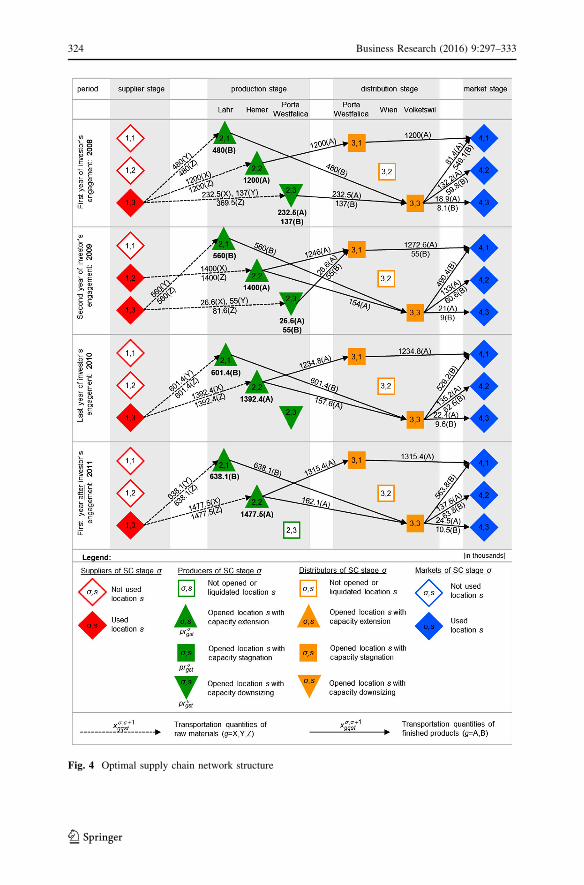
Fig. 4 Optimal supply chain network structure


123

At the beginning of the planning horizon, no surpluses from operations are

available to the investor. Putting the new distribution location in Volketswil into

operation requires EUR 1.175 million (EUR 1 million for opening ? EUR 0.175

million for making related capacities available). Furthermore, initial capacity

changes (capacity expansions in Lahr and Hemer that require EUR 4 million in

each year of the investor’s engagement, and can be balanced with annual cash

inflows of EUR 2 million resulting from capacity downsizing at the production

location in Porta Westfalica until the beginning of 2010) need to be considered. As

financing through two credits (summed up to EUR 1 million, which is equal to the

credit limit of this period) is not sufficient for the purposes mentioned above, the

investor is advised to provide additional funds of EUR 2.175 million to the

company to obtain increasing FTEs in the future. The credits must be repaid after

2 years (EUR 0.25 million) and 3 years (EUR 0.75 million), respectively. After the

first period (i.e., at the beginning of the year 2009), the net operating profit after

taxes is EUR 60.447 million. It is adjusted for regular payments of the

aforementioned ongoing capacity changes (balanced to cash outflows of EUR 2

million). Taking into account two new credits (EUR 0.25 million for 1 year and

EUR 0.75 million for 2 years, interest rates contain risk premium due to the current

total debt of EUR 2 million), a cash outflow to the investor of EUR 59.447 million

is possible. After the second time period (i.e., at the beginning of the year 2010) the

tax shield becomes relevant for determining the net operating profit after taxes of

EUR 61.994 million, as interests of EUR 0.058 million must be paid for two

expiring loans (repayment amount of EUR 0.5 million). Simultaneously, a new loan

(credit amount of EUR 0.75 million, interest rate 2 % p.a. ? risk premium 7.5 %

p.a. due to a current total debt of EUR 2.25 million and the debt limit of EUR 3

million) is taken out. The FTE of EUR 60.244 million results. After the following

time period, the engagement of the investor ends. Last decisions on the adjustment

Table 1 Calculation of FTE (in EUR million)

Beginning

of 2008

Beginning

of 2009

Beginning

of 2010

End of

2010

End of 2011 and

following years

Operating cash flow 93.282 95.727 89.416 95.873

Interest payments for credits -0.000 -0.058 -0.319

Taxes (tax rate 35.2 %) -32.835 -33.676 -31.362 -33.747

Net operating profit after taxes 60.447 61.994 57.735 62.125

Credit f12 (interest rate 6.9 % p.a.) 0.250 -0.250





Location investments -1.000

Location disinvestments 2.700

Capacity (dis-)investments -2.175 -2.000 -2.000 -4.000

FTE 22.175 59.447 60.244 54.185 62.125


123

of the network structure are possible at this point in time (end of the year 2010). In

particular, there are cash inflows of EUR 2.7 million resulting from the liquidation

of the production location in Porta Westfalica. As the rest of the configuration

remains untouched (i.e., there are no further closings of locations), ongoing

operations are ensured after the investor’s engagement. Three outstanding loans

(summed up to EUR 2.25 million) are repaid, the related interests (summed up to

EUR 0.319 million) are relevant for the calculation of the tax shield. Due to a net

operating profit after taxes of EUR 57.735 million, a last cash outflow to the

investor of EUR 54.185 million is possible. Using the given network structure that

would be available to the new holders after the investor’s engagement, a net

operating profit after taxes of EUR 62.125 million could be generated per year. As

the latter is assumed to be a perpetuity, a residual value of EUR 460.19 million

(valid at the end of the year 2010) can be calculated.

The aforementioned optimal solution is based on the assumption that the investor

is able and willing to provide additional funds at the beginning of his engagement

for restructuring. However, if the investor would only be interested in positive

payouts during the engagement (which can easily be implemented by adding non-

negativity constraints for FTE), it can be shown that the company would be cash-

constrained, which is preventing potential ‘‘growth activities’’. In particular, the

maximum present value of equity would decrease to EUR 431.056 million.

Considering the corresponding optimal network structure, the investor would be

forced to cease from production in Porta Westfalica with immediate effect. In

addition, the opening of the new distribution location in Volketswil must be

postponed to the beginning of 2009. Due to the resulting lack of storage capacity,

considerable delivery shortages would be expected during the first time period of the

investor’s engagement—arising especially in the second product group ‘‘tubs’’,

moreover, the Swiss market would be completely unsatisfied. Occurring overca-

pacities at the location in Lahr are used for the production of tubs that are

transferred to the second time period by time overlapping storage. Although the

demand is expected to be satisfied completely after the first year of the investor’s

engagement, an overall percentage of demand coverage of 95.1 % results.

Additionally, we tested the alternative model formulation characterized by the

usage of capacity levels instead of capacity profiles, which results from

implementing the alternative configuration constraints (48)–(56) in the remaining

model (1)–(13), (23)–(47) that is adjusted by the capacity level index. With regard

to the aforementioned case study, the three former capacity profiles being applicable

to all of the locations were split up (according to the given data from the case study)

into nine capacity levels for the plant locations and seven capacity levels for the

warehouse locations. As expected due to the possibility of selecting any sequences

of maximum capacity (which include undesired or even infeasible developments),

the computation time drastically increases. Thus, the computation (performed on the

same aforementioned hardware and software) was aborted after 24 h. The best

present value of equity that was found by then was EUR 454.161 million. However,

a huge gap of 734 % was valid at the same time.


123

7 Scenario analysis

In addition to the case study (see Sect. 6) alternative scenarios were prepared in

order to evaluate the stability of the solution. In particular, the consequences of

considering different discounting rates, uncertain demand as well as additional

sustainability requirements are analyzed. Except the subject of analysis, the test

instances of the scenarios are based on the same parameters as in the case study.

Moreover, the same high-performance software and hardware with the same settings

were used for the computations. As a result, the computation time (CT in seconds),

the cash flows to/from the investor during his 3-year engagement (FTE0, FTE1,

FTE2 and FTE3 in EUR million), the expected annual cash outflow after his

engagement determining the residual value (FTE4 in EUR million), the present

value of equity (VEQ in EUR million) and the overall percentage of demand

coverage (COV in %) were recorded.

The first scenario analysis is related to the challenge of determining accurate

discounting rates (to consider the time value of money and risk premium) and the

potential impact of misspecified discounting rates on optimal decisions. This is

especially important due to the bottom-up beta (see Sect. 5), which is not based on

the company’s share prices, but on an industry average. For this reason, we created

eight test instances with discounting rates that are near to rEQ calculated for the case

study (13.5 %). In particular, discounting rates of 13.1–13.4 % were used for the

four instances R1 to R4, and discounting rates of 13.6–13.9 % were used for the

other four instances R5 to R8.

Although the discounting rate chosen within the aforementioned intervals

determines the present value of equity and the residual value (and thus, the selling

price of the company), we found out that it has no impact on the optimal network

structure and the FTE realizable (Table 2) during the investor’s engagement. As a

consequence, slight inaccuracies or uncertainties while calculating the cost of equity

can be neglected in our case.

As the capital withdrawal by the investor can easily decrease the flexibility of the

SC network, and thus, make it more vulnerable to unexpected changes in the

business environment, a second scenario analysis is taken to determine the effects of

fluctuations in demand. Instead of the expected demand used in the case study, a

uniform integer random number between the following lower and upper bounds was

generated by the optimization software D11t 2 1200; 1400½ �; D21t 2 500; 600½ �;D12t 2 130; 140½ �; D22t 2 50; 70½ �; D13t 2 10; 30½ �; D23t 2 5; 15½ �; 8t ¼ 1; . . .; 4within all of the following 25 test instances (No. D1–D25). The other parameters

of the case study remained unchanged. The results are presented in Table 3.

It becomes obvious that the present value of equity is in the range between EUR

427.938 million and EUR 456.654 million. Regardless of the test instance, the

company is able to cover more than 99 % (on average more than 99.9 %) of the

overall demand despite the investor’s payout claims. All instances were com-

putable without a considerable expenditure of time.

The case study also reveals that supply chain planning is subordinated to the

investor’s payout claims. This may cause conflict of interests. Thereby, the investor


123

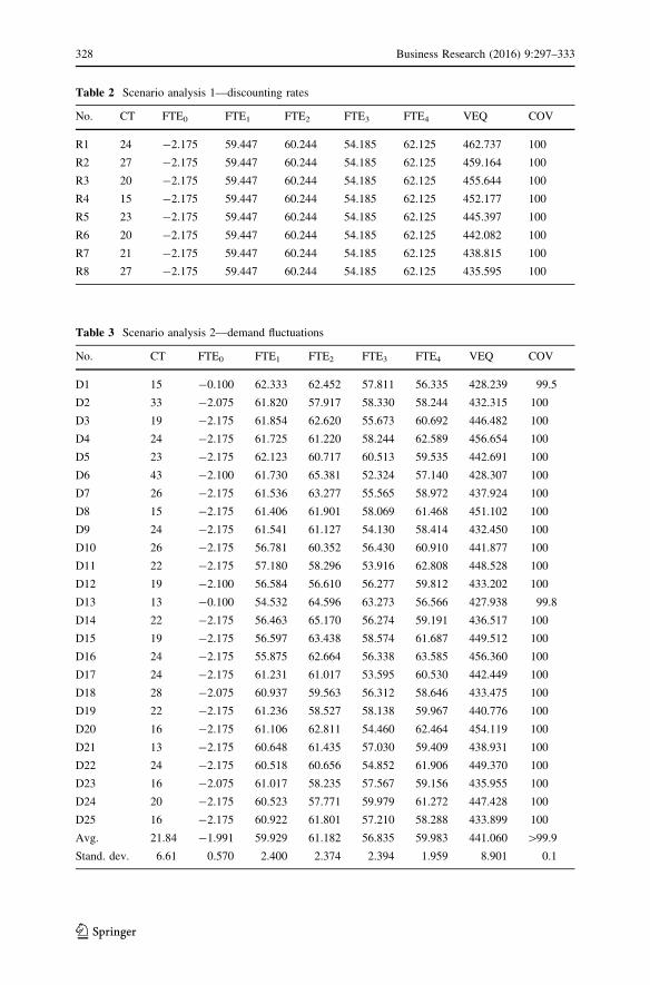
Table 2 Scenario analysis 1—discounting rates

No. CT FTE0 FTE1 FTE2 FTE3 FTE4 VEQ COV

R1 24 -2.175 59.447 60.244 54.185 62.125 462.737 100

R2 27 -2.175 59.447 60.244 54.185 62.125 459.164 100

R3 20 -2.175 59.447 60.244 54.185 62.125 455.644 100

R4 15 -2.175 59.447 60.244 54.185 62.125 452.177 100

R5 23 -2.175 59.447 60.244 54.185 62.125 445.397 100

R6 20 -2.175 59.447 60.244 54.185 62.125 442.082 100

R7 21 -2.175 59.447 60.244 54.185 62.125 438.815 100

R8 27 -2.175 59.447 60.244 54.185 62.125 435.595 100

Table 3 Scenario analysis 2—demand fluctuations


D1 15 -0.100 62.333 62.452 57.811 56.335 428.239 99.5

D2 33 -2.075 61.820 57.917 58.330 58.244 432.315 100

D3 19 -2.175 61.854 62.620 55.673 60.692 446.482 100

D4 24 -2.175 61.725 61.220 58.244 62.589 456.654 100

D5 23 -2.175 62.123 60.717 60.513 59.535 442.691 100

D6 43 -2.100 61.730 65.381 52.324 57.140 428.307 100

D7 26 -2.175 61.536 63.277 55.565 58.972 437.924 100

D8 15 -2.175 61.406 61.901 58.069 61.468 451.102 100

D9 24 -2.175 61.541 61.127 54.130 58.414 432.450 100

D10 26 -2.175 56.781 60.352 56.430 60.910 441.877 100

D11 22 -2.175 57.180 58.296 53.916 62.808 448.528 100

D12 19 -2.100 56.584 56.610 56.277 59.812 433.202 100

D13 13 -0.100 54.532 64.596 63.273 56.566 427.938 99.8

D14 22 -2.175 56.463 65.170 56.274 59.191 436.517 100

D15 19 -2.175 56.597 63.438 58.574 61.687 449.512 100

D16 24 -2.175 55.875 62.664 56.338 63.585 456.360 100

D17 24 -2.175 61.231 61.017 53.595 60.530 442.449 100

D18 28 -2.075 60.937 59.563 56.312 58.646 433.475 100

D19 22 -2.175 61.236 58.527 58.138 59.967 440.776 100

D20 16 -2.175 61.106 62.811 54.460 62.464 454.119 100

D21 13 -2.175 60.648 61.435 57.030 59.409 438.931 100

D22 24 -2.175 60.518 60.656 54.852 61.906 449.370 100

D23 16 -2.075 61.017 58.235 57.567 59.156 435.955 100

D24 20 -2.175 60.523 57.771 59.979 61.272 447.428 100

D25 16 -2.175 60.922 61.801 57.210 58.288 433.899 100

Avg. 21.84 -1.991 59.929 61.182 56.835 59.983 441.060 [99.9

Stand. dev. 6.61 0.570 2.400 2.374 2.394 1.959 8.901 0.1


123

faces a trade-off between cash outflows and sustainability requirements. The latter

concern the reputation of the company or the quality of products. Both of these

aspects can be (additionally to the expected perpetuity of payouts) relevant while

negotiating the selling price of the company after the investor’s engagement. With

regard to the reliability of suppliers, it may be preferable to maintain previous

supply relationships. For this reason, we analyze consequences of continuing

cooperation with the supplier in Hemer (No. S1) or Hettstedt (No. S2) during the

whole planning horizon. Additionally, we focus on the closing of the production

location in Porta Westfalica, which would be optimal due to the aforementioned

solution at the end of the investor’s engagement. In order to prevent the loss of

know-how and human capital, the continued operation of the location with capacity

downsizing (No. S3) or even capacity stagnation (No. S4) could be taken into

account. The results are presented in Table 4.

Both alternatives regarding supplier selection only result in negligible changes of

the present value of equity. Even the considerations with regard to the continued

production in Porta Westfalica lead to changes that are in the range of those that

may be caused by demand fluctuations. Again, all test instances were swiftly

computable.

8 Conclusion

The aforementioned case study is a representative of an increasing economic

phenomenon. In case that a solvency problem arises, which can either be caused by

management failures or the general economic situation, then often institutional

investors (e.g., private equity companies) take over well-established businesses for a

limited period of time. Therewith, the shareholders connect return expectations,

which have to be satisfied by regular payouts taken from profits. Even though there

are examples where existing enterprises were closed down after the takeover, the

continuation of supply chain operations should be a primary goal in accordance with

political and social requests, as it guarantees ongoing returns.

To reach the aforementioned goal, a non-linear flow-to-equity discounted cash

flow model for the coordination of the annual payouts to an investor during his

engagement with SC planning (i.e., location liquidations and openings, capacity

adjustments, sales market and supplier selection, SC operations) and financial

planning is proposed in this paper. The two-phase approach additionally considers

operations that would be possible by using the network structure resulting at the end

Table 4 Scenario analysis 3—sustainability


S1 20 -2.175 59.440 60.212 54.168 62.111 448.645 100

S2 20 -2.175 59.414 60.244 54.156 62.121 448.693 100

S3 24 -2.175 59.447 60.244 53.485 60.505 440.076 100

S4 41 -2.175 59.286 59.938 53.036 59.995 436.806 100


123

of the investor’s engagement. Our objective (maximization of the present value of

equity) also covers the residual value of the expected perpetuity of payouts. In

contrast to data-driven approaches that can be found in the literature in this field, we

model relevant relationships between annual decisions by a system of interdepen-

dent constraints. In particular, these decisions comprise transactions on the capital

market that are realistically influenced by the overall debt limit of the company and

the current total debt within the time periods of the engagement. Due to changing

market situations, duration-dependent interest rates taking into account the specific

time periods the transactions start and end are considered. Resulting trade-offs

between financing volume, interest payments and tax shield are captured.

It becomes obvious that the problem outlined above is challenging due to its

complexity. However, our computations using high-performance software and

hardware revealed that the usage of capacity profiles (which represent feasible or

even desirable sequences of capacity levels, and are alternatively selectable by the

network managers) leads to the fact that the case study of the German sanitary

company could be solved to optimality within seconds. The same applies to all of

the test instances in our scenario analysis, which was conducted to capture

fluctuations in demand, uncertainties in the determination of discounting rates as

well as the consideration of sustainability requirements. By implementing one of

our aforementioned solutions, it can be supposed that the business problems of the

company taken over by the institutional investor could have been prevented or at

least mitigated.

Further research can address the following aspects: As far as a reliable estimate is

possible, growth rates of the company after the investor’s engagement can be taken

into account while maximizing the present value of equity within the FTE approach.

With respect to the limited access to funds, alternative forms of financing can be

added. For capturing international issues of network planning, effects of different

exchange rates and customs duties may be included. Considerations on modeling

may also focus on the subjectivity of valuation, i.e., the investor’s individual

decision field and targets. Finally, the coordination of annual decisions resulting

from our proposed model with continuous-time short-term planning at the locations

can be implemented.

Open Access This article is distributed under the terms of the Creative Commons Attribution 4.0

International License (http://creativecommons.org/licenses/by/4.0/), which permits unrestricted use, dis-

tribution, and reproduction in any medium, provided you give appropriate credit to the original

author(s) and the source, provide a link to the Creative Commons license, and indicate if changes were

made.

References

Amid, A., S.H. Ghodsypour, and C. O’Brien. 2009. A weighted additive fuzzy multiobjective model for

the supplier selection problem under price breaks in a supply chain. International Journal of

Production Economics 121(2): 323–332.

Amiri, A. 2006. Designing a distribution network in a supply chain system: Formulation and efficient

solution procedure. European Journal of Operational Research 171(2): 567–576.


123

http://creativecommons.org/licenses/by/4.0/

Amrani, H., A. Martel, N. Zufferey, and P. Makeeva. 2011. A variable neighborhood search heuristic for

the design of multicommodity production–distribution networks with alternative facility configu-

rations. OR Spectrum 33(4): 989–1007.

Arntzen, B.C., G.G. Brown, T.P. Harrison, and L.L. Trafton. 1995. Global supply chain management at

Digital Equipment Corporation. Interfaces 25(1): 69–93.

Ashtab, S., R.J. Caron, and E. Selvarajah. 2014. A binary quadratic optimization model for three level

supply chain design. Procedia CIRP 17: 635–638.

Azad, N., and H. Davoudpour. 2013. Designing a stochastic distribution network model under risk. The

International Journal of Advanced Manufacturing Technology 64(1): 23–40.

Babazadeh, R., J. Razmi, and R. Ghodsi. 2013. Facility location in responsive and flexible sup-ply chain

network design (SCND) considering outsourcing. International Journal of Opera-tional Research

17(3): 295–310.

Baud-Lavigne, B., B. Agard, and B. Penz. 2012. Mutual impacts of product standardization and supply

chain design. International Journal of Production Economics 135(1): 50–60.

Canel, C., and B.M. Khumawala. 2001. International facilities location—a heuristic procedure for the

dynamic uncapacitated problem. International Journal of Production Research 39(17): 3975–4000.

Chakravarty, A.K. 2005. Global plant capacity and product allocation with pricing decisions. European

Journal of Operational Research 165(1): 157–181.

Correia, I., T. Melo, and F. Saldanha-da-Gama. 2013. Comparing classical performance measures for a

multi-period, two-echelon supply chain network design problem with sizing decisions. Computers

and Industrial Engineering 64: 366–380.

D’Auria, C., A. Foglia, and P.M. Reedtz. 1999. Bank interest rates and credit relationships in Italy.

Journal of Banking and Finance 23(7): 1067–1093.

Damodaran, A. 2012. Investment valuation. Hoboken: Wiley.

Ernst, D., and J. Hacker. 2012. Applied international corporate finance, 2nd ed. Vahlen: Munchen.

Fleischmann, B., S. Ferber, and P. Henrich. 2006. Strategic planning of BMW’s global production

network. Interfaces 36(3): 194–208.

Flynn, B., M. Morita, and J. Machuca. 2011. Managing global supply chain relationships. Hershey:

Business Science Reference.

GAMS. 2012. GAMS–the solver manuals. Distribution 23.8. Washington: CreateSpace Independent

Publishing Platform.

Gardner, J.C., C.B. McGowan, and S.E. Moeller. 2012. Valuing coca-cola using the free cash flow to

equity valuation model. Journal of Business and Economics Research 10(11): 629–636.

Grote, K.H., and E.K. Antonsson. 2009. Springer handbook of mechanical engineering. Berlin: Springer.

Guillen-Gosalbez, G., M. Badell, A. Espuna, and L. Puigjaner. 2006. Simultaneous optimization of

process operations and financial decisions to enhance the integrated planning/scheduling of

chemical supply chains. Computers and Chemical Engineering 30: 421–436.

Hahn, G.J., and H. Kuhn. 2012a. Value-based performance and risk management in supply chains: A

robust optimization approach. International Journal of Production Economics 139(1): 135–144.

Hahn, G.J., and H. Kuhn. 2012b. Designing decision support systems for value-based management: A

survey and an architecture. Decision Support Systems 53(3): 591–598.

Hinojosa, Y., J. Puerto, and F.R. Fernandez. 2000. A multiperiod two-echelon multicommodity

capacitated plant location problem. European Journal of Operational Research 123(2): 271–291.

Ho, W., X. Xu, and P.K. Dey. 2010. Multi-criteria decision making approaches for supplier evaluation

and selection: A literature review. European Journal of Operational Research 202(1): 16–24.

Jayaraman, V., R. Srivastava, and W.C. Benton. 1999. Supplier selection and order quantity allocation—a

comprehensive model. The Journal of Supply Chain Management 35(2): 50–58.

Keyvanshokooh, E., M. Fattahi, S.M. Seyed-Hosseini, and R. Tavakkoli-Moghaddam. 2013. A dynamic

pricing approach for returned products in integrated forward/reverse logistics network design.

Applied Mathematical Modelling 37(24): 10182–10202.

Koberstein, A., E. Lukas, and M. Naumann. 2013. Integrated strategic planning of global production

networks and financial hedging under uncertain demands and exchange rates. BuR—Business

Research 6(2): 215–240.

Kouvelis, P., and Rosenblatt, M. J. 2002. A mathematical programming model for global supply chain

management—conceptual approach and managerial insights. In Supply chain management—

models, applications and research directions, ed. J. Geunes, P.M. Pardalos, and H.E. Romeijn,

245–277. Kluwer: Dordrecht.


123

Laınez, J.M., G. Guillen-Gosalbez, M. Badell, A. Espuna, and L. Puigjaner. 2007. Enhancing corporate

value in the optimal design of chemical supply chains. Industrial and Engineering Chemistry

Research 46: 7739–7757.

Lavaja, J., A. Adler, J. Jones, T. Pham, K. Smart, D. Splinter, M. Steele, and M.J. Bagajewicz. 2006.

Financial risk management for investment planning of new commodities considering plant location

and budgeting. Industrial and Engineering Chemistry Research 45(22): 7582–7591.

Longinidis, P., and M.C. Georgiadis. 2011. Integration of financial statement analysis in the optimal

design of supply chain networks under demand uncertainty. International Journal of Production

Economics 129(2): 262–276.

Mandl, G., and K. Rabel. 1997. Unternehmensbewertung. Wien: Ueberreuter.

Melo, M.T., S. Nickel, and F. Saldanha-da-Gama. 2005. Dynamic multi-commodity capacitated facility

location: A mathematical modeling framework for strategic supply chain planning. Computers and

Operations Research 33(1): 181–208.

Melo, M.T., S. Nickel, and F. Saldanha-da-Gama. 2009. Facility location and supply chain

management—a review. European Journal of Operational Research 196(2): 401–412.

Morash, E.A., and S.R. Clinton. 1998. Supply chain integration: customer value through collaborative

closeness versus operational excellence. Journal of Marketing Theory and Practice 6(4): 104–120.

Ouhimmou, M., S. D’Amours, R. Beauregard, D. Ait-Kadi, and S. Singh Chauhan. 2008. Furniture supply

chain tactical planning optimization using a time decomposition approach. European Journal of

Operational Research 189(3): 952–970.

Ramezani, M., M. Bashiri, and R. Tavakkoli-Moghaddam. 2013. A new multi-objective stochastic model

for a forward/reverse logistic network design with responsiveness and quality level. Applied

Mathematical Modelling 37(1–2): 328–344.

Rong, A., R. Akkerman, and M. Grunow. 2011. An optimization approach for managing fresh food

quality throughout the supply chain. International Journal of Production Economics 131(1):

421–429.

Sadjady, H., and H. Davoudpour. 2012. Two-echelon, multi-commodity supply chain network design

with mode selection, lead-times and inventory costs. Computers and Operations Research 39(7):

1345–1354.

Sahling, F., and A. Kayser. 2016. Strategic supply network planning with vendor selection under

consideration of risk and demand uncertainty. Omega 59: 201–214.

Saunders, A., and L. Schumacher. 2000. The determinants of bank interest rate margins: an international

study. Journal of International Money and Finance 19(6): 813–832.

Schmidlin, N. 2014. The art of company valuation and financial statement analysis. Chichester: Wiley.

Selim, H., and I. Ozkarahan. 2008. A supply chain distribution network design model: An interactive

fuzzy goal programming-based solution approach. The International Journal of Advanced

Manufacturing Technology 36(3): 401–418.

Shapiro, J.F. 2004. Challenges of strategic supply chain planning and modeling. Computers and Chemical

Engineering 28(6–7): 855–861.

Sharpe, W.F. 1964. Capital asset prices: A theory of market equilibrium under conditions of risk. The

Journal of Finance 19(3): 425–442.

Steinrucke, M. 2011. An approach to integrate production-transportation planning and scheduling in an

aluminium supply chain network. International Journal of Production Research 49(21): 6559–6583.

Steinrucke, M., and M. Jahr. 2012. Tactical planning in supply chain networks with customer oriented

single sourcing. The International Journal of Logistics Management 23(2): 259–279.

Steinrucke, M. 2015. Integrated production, distribution and scheduling in the aluminium industry: A

continuous-time MILP model and decomposition method. International Journal of Production

Research 53(19): 5912–5930.

Steinrucke, M., and W. Albrecht. 2016. Quantitative decision support for network integration of start-up

companies. International Journal of Globalisation and Small Business 8(1): 73–99.

Taaffe, K., and J. Geunes. 2004. Models for integrated customer order selection and requirements

planning under limited production capacity. In Supply chain and finance, ed. P.M. Pardalos, A.

Migdalas, and G. Baourakis, 315–344. Singapore: Gainesville.

Taaffe, K., J. Geunes, and H.E. Romeijn. 2008. Target market selection and marketing effort under

uncertainty—the selective newsvendor. European Journal of Operational Research 189(3):

987–1003.

Tofighi, S., S.A. Torabi, and S.A. Mansouri. 2016. Humanitarian logistics network design under mixed

uncertainty. European Journal of Operational Research 250(1): 239–250.


123

Van Roy, T.J., and D. Erlenkotter. 1982. A dual-based procedure for dynamic facility location.

Management Science 28(10): 1091–1105.

Wilhelm, W., D. Liang, B. Rao, D. Warrier, X. Zhu, and S. Bulusu. 2005. Design of international

assembly systems and their supply chains under NAFTA. Transportation Research Part E 41(6):

467–493.

Yi, G., and G.V. Reklaitis. 2004. Optimal design of batch-storage network with financial transactions and

cash flows. AIChE Journal 50(11): 2849–2865.


123

a flow-to-equity approach to coordinate supply chain

Documents