NASA TECHNICAL NOTE N A S A TN_ D-5782-e. 1

A FINITE ELEMENT APPROACH TO THE STRUCTURAL INSTABILITY OF BEAM COLUMNS, FRAMES, AND ARCHES

by JeweZZ M . Thomm 8 i

George C. MarshaZZ Space FZight Center 1

Marsh&, Ah . 35812

NATIONAL AERONAUTICS AND SPACE ADMINISTRATION WASHINGTON, D. C. M A Y 1970

https://ntrs.nasa.gov/search.jsp?R=19700017258 2018-06-16T10:21:01+00:00Z

TECH LIBRARY KAFB, NM

llllllllllllllllllllllrllllllllll~llllll-~~~

1. REPORT NO. GOVERNMENT ACCESSION NO. 0132513 -NASA TN D-5782 I I 4. T I T L E AND SUBTITLE 15. REPORT DATE

A Finite Element Approach to the Structural Instability of 16: PzO:tz: ORGANIZATION CODE Beam Columns, Frames, and Arches

7. AUTHOR(S)

Jerrell M. Thomas 9. PERFORMING ORGANIZATION NAME AN0 ADDRESS

George C. Marshall Space Flight Center Marshall Space Flight Center, Alabama 35812

12. SPONSORING AGENCY NAME AN0 ADDRESS

National Aeronautics and Space Administration Washington, D.C. 20546

~~

15. SUPPLEMENTARY NOTES

Prepared by Astronautics Laboratory Science and Engineering Directorate

16. ABSTRACT

i8 . PERFORMING ORGANIZATION REPOR r M-351

10. WORK U N I T NO.

981-10-10-0000-50-00-08 11 1. CONTRACT OR GRANT NO.

13. T Y P E OF REPOR-; & PERIOD COVERE

I Technical Note SPONSORING AGENCY CODEI'-.I.

I

A nonlinear s t i fhess matrix for a beam column element subjected to nodal forces and to a uniformly distributed load is developed from the principle of virtual displacements and the bifurcation theory of elastic stability. Three cases of applied load behavior a r e considere The buckling load of a uniform circular arch is calculated as an example.

17.' KEY WORDS 18. OlSTRlBUT lON S T A T E M E N T

Unclassified - Unlimited

19. SECURITY CLASSIF . (of this report) 20. SECL IF. (of this pege) 21. NO. OF PAGES 22. PRICE*i Unclassified I Unclassified 58 $3.00

TABLE OF CONTENTS

INTRODUCTION.... ................................... 1

G E N E R A L T H E O R Y . . . . . . . . . . . . . . . . . . . . . . . . . . . . . . . . . . . . 3 Basic Assumptions and Limitations .. ... .... . .. . . . . . . . . . 3 Method of Analysis .. . .. .... .. .. .... . . . . .. .... . . . .. 4 Development of Element Stiffness Matrix .. .. . . . . . . .. . .... 5

Description of Element . .. ... . .. .. . . . . . . . . . .. . . 5 Displacement Functions . . . . . ..... . . . . .... .. . . . 5 Development of Equilibrium Equations .. . . . .. ... . . . . 7 Bifurcation Theory of Instability . . . . . . . . .. .. . . . . . . 16

NConventional Stiffness Matr ix , K .. . . . . . . . . .. . . . . . 20 Geometric Stiffness Matrix, ,G . . .. . . . . . . . . . . . . . . . 21 Load Behavior Matrix, L. . . . . . . . . . . . .. . . . . . . .. . 28

N

Coordinate Transformation . . . .. .. . . . . . . . . . . .... ... . . 32 Master Stiffness Matr ix . ... . . . . .. . . .. .. . . . . . . . . .. . . . 35 Stability Criterion . .. . . . . . . . . . . . . . . . . . . . . . . .. . .... 37 Primary Equilibrium State. . .. .. . . . . .. . .. . . . . . ... . . . . 38

APPLICATIONOF THE THEORY ........................... 39

EXAMPLE P R O B L E M . . . . . . . . . . . . . . . . . . . . . . . . . . . . . . . . . . . 41

C O N C L U S I O N S . . . . . . . . . . . . . . . . . . . . . . . . . . . . . . . . . . . . . . . . 44

REFERENCES ........................................ 46

iii

111l l1 l l I l l I I1 I I

L I S T OF ILLUSTRATIONS

F i g k e Title Page

i. Beam Column Element ............................. 5

2. Loads Remain Normal to Element. ..................... 10

3. Loads Remain Parallel to Original Direction . . . . . . . . . . . . . . 11

4. Loads Remain Directed Toward a Fixed Point . . . . . . . . . . . . . 12

5. Coordinate Transformation .......................... 32

6. General Structure ................................ 35

7. Uniform Circular Arch. ............................ 42

L I S T OF TABLES

Table Title Page

I. Comparison of Arch Buckling Loads .................... 44

ACKNOWLEDGMENT

This analysis was done at the suggestion of Dr. C. V. Smith of Georgia Institute of Technology. M r . John Key assisted in checking certain portions of the analysis. Mr . Dan Roberts of Computer Sciences Corporation did all of the programming for the example problem. The contributions of these people a r e gratefully acknowledged.

iv

L I S T OF SYMBOLS

Symbol Meaning

A Cross sectional area of element

E Modulus of elasticity of material

F Force applied to element node -F Force applied to element node referenced to undeformed

element coordinate system

+ F Proportionality constants between forces, F , and lateral

load, p

G = [GI Geometric stiffness matrix defined by equation (46)N

I Moment of inertia of element c ross section

K = [K] Conventional stiffness matrix defined by equation (45) N

NKf= [ Kf]* Total element stiffness matrix (see equation (44))

K= [ K] Element stiffness matrix in global coordinate systemN

KO = E KO1 Nonlinear stiffness matrix defined by equation (91)N

L Length of element

L = [L] Load behavior stiffness matrix N

kF = LF1 Nodal force behavior stiffness matrix

L ‘ILJ Lateral load behavior stiffness matrix“P

1 Distance from element node to point through which the FXnodal forces are directed

V

L I S T OF SYMBOLS (Continued)

Symbol Meaning

M Bending moment applied to element node

M = M Bending moment applied to element node referenced to undeformed element coordinate system

m, n Unit vectors in element coordinate system

iii, n Unit vectors in global coordinate system

P Lateral load applied to element

Q Nodal force o r moment

Q = { Q } Column vector of nodal forces and momentsN

g = {a} Column vector of nodal forces and moments referenced to global coordinate system

Nodal displacement o r rotation

Column vector of nodal displacements

Column vector of nodal displacements in global coordinate system

R Distance from element centerline to point through which lateral forces are directed; also radius of circular arch

T = [TI Coordinate transformation matrix defined by equation (81)N

U Strain energy of the element

U Displacement in x direction

-U Displacement in Z direction

vi

Symbol

V

W

-W

x, z

z,z

CY

P

Y

6U, 6V

k

E xx

9

K

UX

dl

w

LIST OF SYMBOLS (Continued)

Meaning

Volume of the element

Displacement in z direction

Displacement in E direction

Element coordinates

Global coordinates

Constant coefficient

Angle between element and global coordinate systems

Displacement functions defined by equation ( 6 )

Change in strain energy, virtual work of external forces

Strain of element in x direction at any point

Strain of element midsurface in x direction

Rotation of element node

Curvature of beam element centerline

Stress in x direction at any point in the element

Displacement functions defined by equation ( 5 )

Unit rotation vector

vii

Symbol

Subscript

1, 2

9-x; r m c

1Superscript

0

I

-1

T

L I S T OF SYMBOLS (Concluded)

Meaning

Matrices defined by equations (55) through (61)

Meaning

Denotes left and right nodes respectively of the elements; also denotes a particular displacement function, y

Denotes a particular @ displacement function

Denotes a particular element of a general structure

Denotes a particular node of the element or one of the displacement functions, y or @

Indicates no summation on double subscript, i

Direction of the coordinates x and z

Fi r s t and second derivatives with respect to x

Meaning

Denotes displacements of the structure just prior to buckling

Denotes displacements of the structure just after buckling

Inverse of a matrix

Transpose of a matrix

viii

A FINITE'ELEMENT APPROACH TO THE STRUCTURAL INSTAB l L l T Y OF BEAM COLUMNS,

FRAMES, AND ARCHES

SUMMARY

From the principle of virtual displacements and the bifurcation theory of elastic stability a stiffness matrix is developed for a beam column element with shear , moment, and axial load applied to the ends ( nodes) of the element and a uniformly distributed load applied along the span of the element. The stiffness matrix developed relates the forces applied at the nodes to the displacements of the nodes and is a function of the magnitude of the applied load. Three types of behavior of the applied loads are considered as separate cases. These are: the loads remain normal to the deformed element; the loads remain parallel to their original direction; and, the loads remain directed toward a fixed point.

A method is given for using the element stiffness matrix to predict the buckling load for a structure which may be represented by beam column elements. A s an example, the buckling load of an arch for each of the three load-behavior cases is calculated and compared to known solutions.

INTRODUCTION

In recent years interest in the solution of structural problems by the finite element method has greatly increased. This interest can be attributed to the fact that the digital computer has made possible the solution of a great num­ber of complex, yet practical, problems by this method.

Those active in publishing results in the field include a group at the University of Washington and The Boeing Company [ 1-91, J. H. Argyris at the University of London [ I O , 111, and R. H. Gallagher and his associates at Bell Aerosystems Company [ 12- 141.

Basically the method consists of representing an actual structure by an idealized structure made up of elements for which relationships between the forces applied to points (nodes) on the boundary of the element and the displace­ments of the nodes is known. This relationship is conveniently represented by

an element stiffness matrix. If all of the element stiffness matrices are trans­formed to a common (global) coordinate system, the sum of.forces applied to the elements meeting at each node is equated to the externally applied force at that node, and the displacements of elements which meet at each node a r e equated, a s e t of equations relating the externally applied forces to the nodal displacements results. When this s e t is expressed in matrix form, the matrix relating the ex­ternally applied forces to the nodal displacements is called the master stiffness matrix. Then for any given combination of known applied external forces and nodal displacements the above relationships may be algebraically manipulated to determine internal loads and displacements throughout the structure.

Once a sufficient variety and quality of element stiffness matrices a r e available to idealize a particular structure, the remainder of the above procedure to solve a particular problem becomes tedious but quite mechanical. Hence the advantage of the computer in solving such problems is obvious.

Although the use of such techniques in solving complex structural prob­lems is now an everyday occurrence, a great deal of developmental activity in the field still persists for several reasons. First, there is no such thing as a correct stiffness matrix for a particular element which excludes other stiffness matrices for that same element as incorrect. A number of correct stiffness matrices may be developed for the same element if different assumptions a re made for the derivation. Each of these matrices may have its own advantages for some particular application and all of them may converge to identical answers if the structure to be analyzed is broken into small enough elements. It is the search for the most advantageous element for particular applications or for all-inclusive elements which gives r i s e to much of the current research.

Second, many derivations have been based on geometrical considerations only and have sometimes led to incorrect stiTfness matrices o r matrices with poor convergence characteristics. The recent trend has been to base derivations on basic elasticity principles and to use more care in assuring that adjacent element deformations conform to each other not only a t the nodes but along the complete boundary 15, 15-19].

Third, extension of the finite element techniques to include a larger class of problems has received a great deal of recent attention. In particular, the solution of nonlinear problems including large deformations and structural instability has been of interest [ 1-3, 5, 8, 9, 13-15, 17, 201.

2

I

This report was motivated to some extent by all three of the above con­siderations. The objective was to develop a beam column element, beginning with fundamental principles, which would account for the applied load behavior and could be used for structural stability analysis.

It is assumed that the reader is familiar with the conventional matrix and index notation used throughout the report. Since there is no stringent space limitation, the work is presented in an unusual amount of detail with the pre­sumption that the development could serve as a guide for the development of curved or three-dimensional elements.

GENERAL THEORY

Basic Assumptions and Limitations

The usual Euler-Bernoulli beam assumptions a r e made for developing the beam column element stiffness matrix. These are basic engineering assump­tions and may be listed as follows:

I. The material of the element is homogeneous and isotropic.

2. Plane sections remain plane after bending.

3. The stress-strain curve is identical in tension and compression.

4. Hooke's law holds.

5. The effect of transverse shear is negligible.

6 . The deflections are small compared to the cross sectionai dimensions.

7. The loads act in a single plane passing through a principal axis of inertia of the cross section.

8. No initial curvature of the element exists.

9. No local type of instability will occur within the element.

I O . Loads are applied quasi-statically.

3

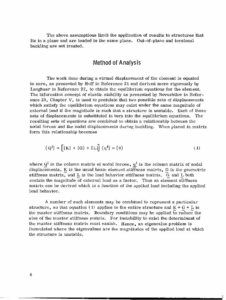
The above assumptions limit the application of results to structures that lie in a plane and are loaded in the same plane. Out-of-plane and torsional buckling are not treated.

Method of Analysis

The work done during a virtual displacement of the element is equated to zero, as presented by Hoff in Reference 21 and derived more rigorously by Langhaar in Reference 22, to obtain the equilibrium equations for the element. The bifurcation concept of elastic stability as presented by Novozhilov in Refer­ence 23, Chapter V, is used to postulate that two possible sets of,displacements which satisfy the equilibrium equations may exist under the same magnitude of external load if the magnitude is such that a structure is unstable. Each of these sets of displacements is substituted in turn into the equilibrium equations. The resulting sets of equations are combined to obtain a relationship between the nodal forces and the nodal displacements during buckling. When placed in matrix form this relationship becomes

where Qi is the column matrix of nodal forces , is the column matrix of nodal displacgments, K is the usual beam element stiffness matrix, G is the geometric

N

stiffness matr ixrand L is the load behavior stiffness matrix. G and L both contain the magnitudezf external load as a factor. Thus an elekent syiffness matrix can be derived which is a function of the applied load including the applied load behavior.

A number of such elements may be combined to represent a particular structure, s o that equation ( I) applies to the entire structure and K + G + L is the master stiffness matrix. Boundary conditions may be applied To r&ucg the s ize of the master stiffness matrix. For instability to exist the determinant of the master stiffness matrix must vanish. Hence, an eigenvalue problem is formulated where the eigenvalues are the magnitudes of the applied load at which the structure is unstable.

4

Development of Element' Stiffness Matr ix

Description of Element. Consider a beam column element as shown in Figure 1 which is subjected to nodal forces and moments and a uniformly dis­tributed load, p, applied along its length. It is desired to determine a stiffness matrix for the element which may be used to calculate the stability of structures made up of such elements. The stiffness matrix is to account for the fact that the components of the nodal forces or distributed load, or both, may be a function of the element displacements. Three cases a r e to be considered: the loads remain normal to the deformed elemeht; the loads remain parallel to their original direction; and, the loads remain directed toward a fixed point.

FIGURE I. BEAM COLUMN ELEMENT

Displacement Functions. If it is assumed that the lateral displacement of the beam element of Figure i may be represented by

and the longitudinal displacement is given by

5

then the six unknown constants, a!i’ may be determined in terms of the nodal

displacements from the element boundary conditions,

w = w i at x = O

w, X

= - e l at x = O

w = w 2 a t x = L

w, X

= -e2 at x = L

u = u i a t x = O

u = u 2 a t x = L .

The resulting displacement functions a r e

w = w i (1 - 3 - + 2 9 + w 2 ( 3 $ 2 $:: L3

+ e , ( - x + 2”” -2)L L2 + e2($ 5)

= w . @.(XI1 1

6

These displacement functions have been used by others for the beam column element (see Reference 5, for example). However, it should be men­tioned that an inconsistency ar i ses when the cubic function is used for the lateral displacement of the present element which has a distributed load. This is illus­trated by taking the third derivative of w, which should be the equation for the shear load on the element, and observing that a constant results. But the ele­ment has a distributed load, and the shear should obviously be a linear function, not a constant. Since the change in shear over the length of an element becomes negligible in the limit as the element becomes smaller and smaller, this incon­sistency is not unacceptable and it will be seen that adequate results are obtained. The correct fourth order function could not be used for w because there is no other boundary condition available for evaluating another constant in equation ( 2 ) . This will be discussed further in the conclusions.

Development of Equilibrium Equations. The element equilibrium equa­tions will now be developed from the principle of virtual displacements,

6 U - 6 V = O ( 7 )

where 6U is the change in strain energy and 6V is the work done by the external forces during a virtual displacement.

For the uniaxial state of stress assumed to exist in a beam the change in strain energy is given by

6U = J ax6 exdv V

Here, E X

is the strain of the beam at any point of the cross section and is given by

where E is the s t ra in of the beam mid-surface, z is the distance of the point in xx the beam from the mid-surface, and

K = W ,xx xx

7

is the beam curvature. The nonlinear strain-displacement relationship

1E xx = u , x + 2 w ’ x 2 + - u ,

x 2

2

is used for the mid-surface strain. The u , ~X

term in this expression is not

known to have been used in previous derivations of nonlinear beam element stiffness matrices. Substituting equations ( 9 ) , ( I O ) , and (11) into equation ( 8 ) ,

6 U = s [,,cxx6t xx

+ E I K xx

6K xx1dx

L

where

d � = 6 u , + d ( i w , ; ) +d(&;) = 6 u , x + w , x 6w, x + u , x 6% x xx X

+ z I u, 2, t u , + w, dw, + u, ~ u , ~ ) + - E I w , ~ ~ ~ w , ~ ]u , ~I w,: + z dx

L X X x x X

8

+ higher order terms. (14)

The virtual work of the external forces acting on the element is given by:

where the force components depend upon the load behavior. Three load behavior cases will be considered.

Case I. Loads Remain Normal to the Deformed Element (Fig. 2)

Pz = P

-pX - - P K x -F = F . + F exi xi z i -i F = F - F e

zi zi xi -i Z. = M.

1 1

Then

9

c

= p cos 9 H p 4 pz I

I

FIGURE 2. LOADS REMAIN NORMAL TO ELEMENT

Case 11. Loads Remain Parallel to Their Original Direction (Fig. 3)

P, = P

p = o X - -Fxi - Fxi -FZi = FZi

M. = M. 1 1

10

I

FIGURE 3. LOADS RENIAIN PARALLEL TO ORIGINAL DIRECTION

6V = Fx1.6u . 1

+ Fz1.dwi + M. 68 . i - s p6wdx (19)l L

Case 111. Loads Remain Directed Toward a Fixed Point (Fig. 4)

Pz = P

PUP, =

- UiFxi = Fx1. + F Z i ~ - WiFZi = FZi - Fxi 1 k.= M.

1 1

Fxi + FZi% 6 ~ .u’) + (FZi - Fxi?)6w i

FIGURE 4. LOADS REMAIN DIRECTED TOWARD A FIXED POINT

12

-u

Substituting equations ( 14), (17) , ( 19), and ( 21) into equation (7), we obtain the following results:

Case I.

I{ [EA(USx + z w , 2 + 3 2)6u,x + EA(u,xw,x)6W,x x 2 'x

+ EIw ,xx 6w, -1 dx = (Fxi ;FZi Bi -)6ui + (FZi - Fxi ,)6wi

Case 11.

dx = F .6u . + F . 6 ~ .+ Misei+ p6wdxxx L

Case 111.

L

From the displacement functions, equations ( 5) and ( 6 )

u, X

= u. 1

y.l ,x

w, X =wi cPi,x (25)

w, xx = wi cPi,- .

13

-

And the above variations can be written,

6u = y . 6Ui 1

-6u, X Yi,x 6ui

6w = Gi6Wi

6WYx = @i,xdWi

- 6w .6WYn - @i,xx i

Upon substituting equations (25) and (26) into equations (22) through (24) and recalling that Oi = wi +2, the following equations are obtained:

Case I.

) 6 u i - ( F zi - Fxi wi + 2)6w i -

Case 11.

- Fx1. 6 u . - F z1.6w.-M.6w i + 2 - p@.6w.dx=O1 1 1 1 1L

14

/

1

L

+( Ju.y.J , X wk qJk,x)'i,x

+ FZi %)hi-U i

PSwi + -u. y. y. 6ui

Case 111.

+ EIw.J @.6wl 1,xx CPj , xx

(FZi - Fxi "') 6wi - Mi 6wi+

R J J 1 (29)

For independent virtual displacements , 6u. and 6wi'

the equilibrium1

equations are obtained from equations (27) through ( 2 9 ) .

Case I.

I 3 j ,xy i ,x + - w w $j k ,x@.

J , Xy i ,x + - u u y2 k 2 k j k ,xy j ,xy i ,x

EAuj yj , x wk CP k , x CP i ,x +EIw.@.J I , = CPj y = - P ( @ i ) ] h L

,

Case 11.

i2 k wj @k,x @. 3[..('jyj,xYi,x +-w J , X yi , ~ + 2 % ~ j ~ k , x ~ j , x ' i , x

L

15

_.. . - . .. .._._ .. -I I I I II111111 I I 111 I ,._..

Case 111. F

I 3bA('j 'j ,x 'i, x + ZWk"j 'k, x 'j ,x 'i, x +;% "j 'k, x 'j ,x 'i, x

W i-- Qzi

+ Fxi -1

= o (35)

Equations (30 ) through ( 3 5 ) a r e the final equilibrium equations for the beam column element.

Bifurcation Theory of Instability. Let a solution of the equilibrium equations be uo woi'

According to the bifurcation concept of instability, at thei'

instability load magnitude there is another set of displacements, arbitrarily close to the first set, which. also satisfies the equations of equilibrium. Denote this second set of nodal displacements by uo

1 t.u1 w? + w1i .i ' i

Upon substituting this new solution into the equilibrium equations, there results for Case I

16

---- -. ........_... ... ..- -. . .,,

k yj , x

@k , x

@i , x

(37)

Similar results are obtained for Cases I1 and 111,

If these equations are expanded, if the q? state terms (which themselves 1

satisfy the equations) are canceled, and if only linear te rms in the arbitrarily small q! state are retained, the following sets of equations result.

1

Case I.

oFA($'j,xyi,x + wji Wkgk,x+. J , X

y.1 ,x + 3Y(:ulyk, x 'j ,x 'i, xJ

+pw!@. y. d x - Fzi 0'i

= O ( 3 8 )J JYX 11 ­

i , x @

k ,x yj , x

+ w ij \

'+.i , x

@.J , X

yk , x

+ EIW!+ J i ,xx +j , xx1dx

+ Fx1.e! -1

= 0 ( 3 9 )

Case 11.

Y.' +W!W0 k @k ,x @.J , X

y.1 , ~ J1 , ~ J

+ 3 q u i yk,xyj , x 'i, x)I dx = 0

17

r 7

~ [ E A ( u ~ w ~ ' i y x 1,x +. J+k , x Yj , x + w ij u kO9. J , X Yk,x + E I W ~ +i,= +j , = J dx

Case 111.

i , x @

k,x yj , x

+ w ij \

' @ .1,x @.J , X

Yk , x

These equations may be expressed in matrix notation sa-a three cases as follows:

o r

[Kil (q'} = ( 0 )

where

[K1] = [ K 1 + [GI+ [Lp] + [LFl

1 8

--- ----- ----------

1s 3EA $yk,xyj,x'i,x dx 1 s EAwL'k,x'j,xYi,x L

1 - I-E A w 0 $ i ,x $k,x yj ,x dx Is EA$$ i ,x @.

J , X yk,xk ' L

[GI (q'} =

for all cases.

I

The L matrices are different for each case. N

Case I.

[Lpl {si} =

[L,l{ql} =

[ L 1 = [L,I=[OlP

Case 11.

Case 111.

(47 1

(48)

(49)

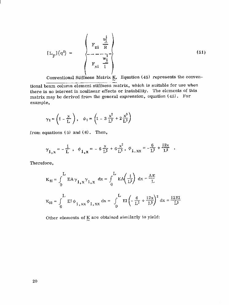
Conventional Stiffhess Matrix 5, Equation (45)represents the conven­

tional beam column e l e m e n t a t r i x , which is suitable for use when there is no interest in nonlinear effects o r instability. The elements of this matrix may be derived from the general expression, equation (45) . For example,

from equations ( 5) and ( 6 ) . Then,

Therefore,

L L 2 I2EId x = EI(-j!$+%) dx=- L3

0 0

Other elements of K a r e obtained similarly to yield:N

20

- -

- -

-- -- --

--

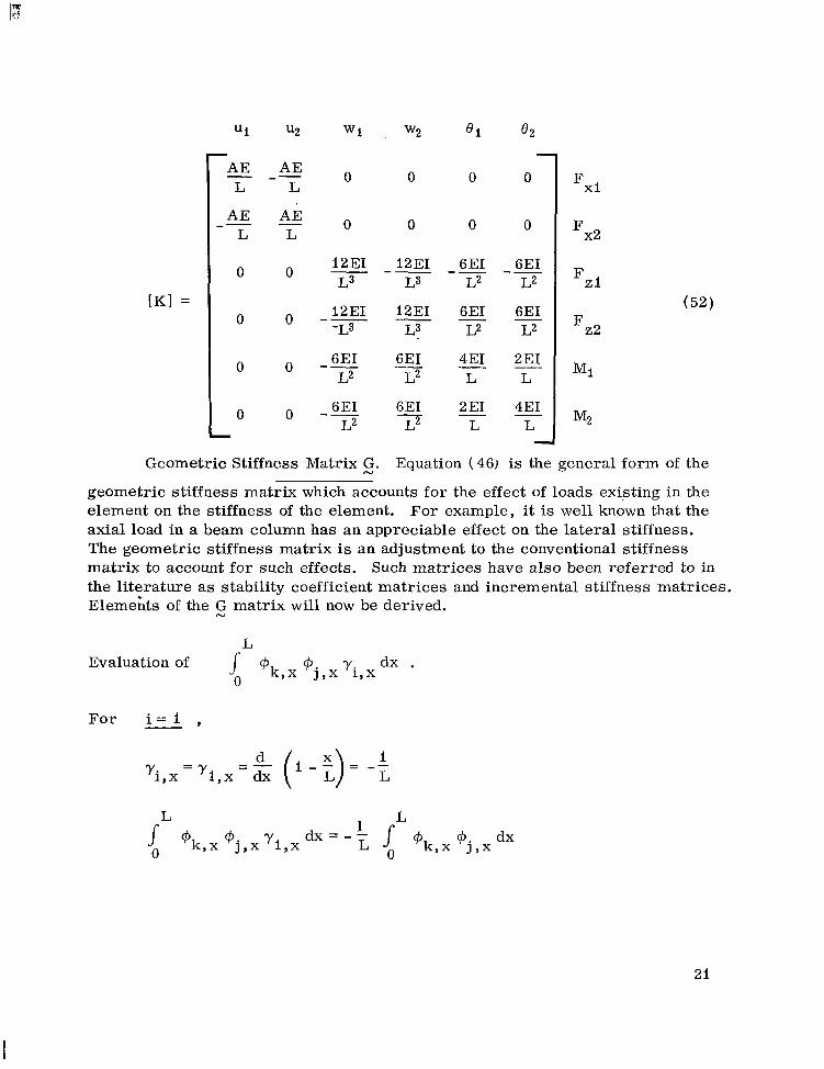
U I uz -

AE L E L L Fxi

AE AE-L L 0 0 0 0 Fx2

12EI 12EI 6EI 6EI-0 0 L3 L3 L2 L2 F Z i

[Kl = 0 0 12EI 12EI 6EI 6EI (52)- - ­

-L3 L3 L2 L2 F Z 2

0 0 MI

0 0 M2-Geometric Stiffness Matrix G. Equation (46) is the general form of the

N -~

geometric stiffness matrix which accounts for the effect of loads existing in the element on the stiffness of the element. For example, it is well known that the axial load in a beam column has an appreciable effect on the lateral stiffness. The geometric stiffness matrix is an adjustment to the conventional stiffness matrix to account for such effects. Such matrices have also been referred to in the literature as stability coefficient matrices and incremental stiffness matrices. Elemehts of the G matrix will now be derived.

N

L Evaluation of

0 @k,x@j , x Yi , x d x .

For i = 1 ,

21

when k = I,j = I ,

For i = 2- 9

d

Other values of j and k are evaluated similarly to yield

22

~ - - - . . - - 1 1 ~ . , ~ . , 1 1 . 1 . 1 1 1 1 1 1 1 1 1 1 1 . 1 111.111111111111.11.11111.1111111111111111111 1111111 II 1111 I I I I I 1111 111 1111111 11111 I I I I 111 I

-- - -

--

--

--

L IOL 'k.x 'j , x Y2 ,x dx= I -I -4 I (54)

0 iOL iOL 30 30

4-30-

L Evaluation of

0 'i,x'j,x 'k,x dx .

For i = I

j = I,k = 1

L

0

when j = I, k = 2 .

6 6-L 5L2 5L2

J ' l , xCpk ,xYj ,xdx = 0 -i

i0L i

IOL

( 5 5 )

1 i __IOL i0L

23

--i -L--IOL IOL

L

.f0 '3,x'k,x'j,x dx =

--I -L--IOL IOL

L dx =

0 '4,x'k,xyjyx

L Evaluation of

0 yk, 'Yj , Yi , dx .

Then,

24

~ . .. .... ,.

--

---- --

----

Evalllation of 1 @. @. y dx . 0 1YX JYX k , x

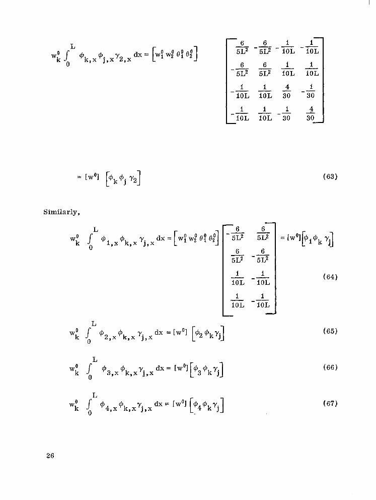
The above matrices a r e now multiplied by the cyo state displacements as indicated in equation (46) , k

- -6 -6 -I -I

5L2 5L2 IOL IOL

6 6 1 I-5L2 5L2 IOL IOL

-I I 4 I-iOL IOL 30 30

25

--

--

--

--

--

L

Similarly,

L r 7

0 0 0 wo s 'I,x'k,x'j,x

dx = [wlw2 el0 e2J k O

26

--I -I I -4 IOL IOL 30 30- L

--6 6-

5L2 5u

6 6-5L2 5L2

I I-IOL i0L

(64)

I I-IOL IOL--

The above matrices a r e combined to form the G matrix (Equation ( 46) ) : N

27

[GI =

Load Behavior Matrix. The effect of applied load behavior on the element stiffness is obtained by adjusting the 5 matrix with the k m a t r i x , where

[ L l = [LP '

1 + [LFl . (75)

The L matrix will now be derived from equations (47) throug,, (51) for each of the t&ee load behavior cases.

Case I.

28

I

--

- -

p

Then,

-- I L L-0 0 2 12 12

I L -A­0 0 2 12 12

0 0 0 . o 0

(761 0 0 0 0 0

0. 0 0 0 0

0 0 0 0- 0 -

L-F may be written directly from equation (48)in view of equations ( 3 8 )

and (39 ) ;

0 0 0 -FZ2

0 0 0

[LFl = P F X l (77)

0 Q 0 "2

0 0 0 0

0 0 0 0

where F's are proportionality constants between the indicated forces and p. The magnitudes of the applied forces' are assumed to remain in a constant ratio to each other and to the lateral load, p, during loading of the element. This

29

--

--

-assumption is made here and in the Stability Criterion section for illustrative purposes. The assumption is easily altered to study buckling under pressure with specified nodal forces or buckling under nodal forces with specified pres sure.

Case 11.

[L 1 = [LFl = io1P

Case 111.

dx

L ="[(x-r+3 X2 x3 ) uj +($ -$) "11R

0

L 0 0 06R

L 0 0 03R

0 [ L

P I ' P

0

0

0

30

II I

--

L may be written directly from equation (51) ;-F

O 0 0 4

F Z 2

R 0 0 4

F X l0 1 0

[LFl = p 4

Fx20 0

1

0 0 0

0I- 0 0

-0

0

0

0

0

0­

31

Coor di nate Transformation

The developments thus far have been in a coordinate system which was oriented so that the x-axis coincides with the element centerline. To combine several elements for solution of a particular problem, it is necessary to obtain the stiffness matrices of the elements in a common or global coordinate system. This system wi l l be denoted by x, z as shown in Figure 5.

FIGURE 5. COORDINATE TRANSFORMATION

The figure shows that vectors in the two coordinate systems transform according to the relationships

m = fi cos p + ii sin p

n = ii cos ,8 - GI sin p

-o = w .

32

Writing in matrix notation, we see that

Thus the displacements and forces of the element transform according to

I -T I FZ i

I *

0 I T F Z 2 I I I G2

33

or

If the nodal forces and displacements are related by the stiffness Ki N

(equation (44)) , then

where Ki has been rearranged to conform to the Q and q matrices. Upon sub-N

stitutini equations (82) and (83) into equation (8z) ,

But in this case,

34

where if is the stiffness matrix of the element in the global coordinate system.N

Master Stiffness Matrix

The stiffness matrix for complete s t ruc ture is obtained by combining the element stiffness matrices in the global coordinate system. This section describes the method of accomplishing this combination.

Consider par t of an overall structure schematically represented by Figure 6. The &.Is in Figure 6 are intended to represent the total load vector

1

FIGURE 6. GENERAL STRUCTURE 35

I

at the point of application,

Load-displacement relationships for each of the three elements in the global coordinate system are expressed from equation ( 87) as follows:

By combining the above relationships with the fact that gi is the same for

both elements b and c, and noting that

and that similar relationships hold for the other nodes, the master stiffness matrix is obtained:

36

I

- ­_--K a i - i . i - l +Eb i - 1 , i - 1 K b i - i , j 0

- - ­0 %i, i - 1 Kbii +Ec i i Kci, i + 1

-0 0 K . tx

c i + l , i K c i + l , i + l d i + l , i t

0 0 0 -_­

-

Note that this is a relationship between the externally applied loads and the nodal displacements of theassembled structure in the global coordinate system.

StabiIity C r i t e r i o n Elements with stiffness matrices of the type given by equation (44) may

be assembled into a master stiffness matrix to represent a structure subjected to the critical (buckling) magnitude of applied loads. Thus,

[[Kl + P [Eol]{G1)= (0)

where,

p[liol = [GI + [Ep] + [E,] 9 ( 9 1 )

and the null matrix of applied external loads indicates that the structural stiffness has vanished under the critical load magnitude ( a physical interpretation of instability). Boundary conditions may be applied to reduce the size of the se t of equations (90) and the new reduced se t again denoted by the equations (90 ) .

The E, G, and matrices above are obtained by assembly of element " "P

matrices as described in the preceding sections, The E matrix is more"F conveniently obtained by direct application of equations (48) and (51) to each node of the assembled structure in the global coordinate system.

A nontrivial solution of equations ( 90) will exist only when the determinant of the matrix + p E, vanishes;

N N

This is an eigenvalue problem where the magnitudes of applied load, p, at which instability will occur are the eigenvalues.

37

111.1111111 111111111 1 1 1 1 1 I I I I I I , I

Pr imary Equil ibr ium State

It should be noted at this point that the foregoing solution is contingent upon a knowledge of the primary equilibrium state. That is, the G matrix can­not be formulated until the qodisplacements are known in terms the applied loads. Given a se t of applied loads, the nonlinear equilibrium equations (30) through ( 3 5 ) may be solved for the qodisplacements. An iterative procedure for incorporating this solution into the stability problem is given in Reference 14.

Another approach which is consistent with many classical stability prob­lem solutions is to linearize equations ( 3 0 ) through (35) for the purpose of obtaining the primary state solution. If this is done these equations become for all three cases

( 9 3 )

A l l t e rms in the above equations have previously been evaluated and expressed in matrix form except the p@.term which is as follows:

1

Y0 -0 \

38

l or 0

0

L-2

{P@> = P L Y

2

L2-12

L2-12

Equations ( 9 3 , 94) may then be expressed in the form

From this expression for each element, the master stiffness matrix for the entire structure is assembled as before. Then for the complete structure,

A further simplification fo r obtaining 9' which has also been used extensively in classical problems is the use of a membrane solution for zo. The structure is assumed to take no loads in bending before buckling. For many practical problems such a solution can readily be obtained by inspection, ele­mentary equilibrium considerations, or from the literature. For simplicity this approach is used in the example problem of this report.

APPLICATION OF THE THEORY

This section is intended to give a step by step approach for applying the theory to the solution of practical problems. For problems with several elements

39

either a general computer program would need to be developed o r a relatively simple computer program for each application could be developed as was done for the example to follow later.

One begins by dividing the structure to be analyzed into discrete elements, the number depending upon the desired accuracy. From the known properties and loading on each element the K matrix can be calculated from equation (52)

N

and the L and L matrices determined from the appropriate equations (76), (77),"P -F (78 ) , (79), o r (80) . Note that the critical magnitude, p, of the applied loading remains as the unknown to be determined.

The qo primary state is now determined from a known membrane solution o r from equztion (97). The K matrix in equation (97) is assembled by using equations (81) and (86 ) to tr&sform elements to the global coordinate system and equation (89) for combining the elements. Boundary conditions a r e applied and equation (97) is solved for qo. Once the qo state is determined the G matrix can be found from equatl'uon (74) , using the definitions (53) throcgh (61) .

The K' matrix defined by equation (44) is now known for each element. These a r e agsembled into a master stiffness matrix by equations (86) and (89 ) , and boundary conditions are applied to the resulting set of equations to obtain equations (90) . Eigenvalues of the characteristic determinant, equations (92), which is obtained from equation (90 ) , a r e the magnitudes of the buckling load. The mode shape for each buckling load c.an be determined by substituting each eigenvalue in turn into equations (90) and solving for the relative amplitudes of displacements, 6

i'

EXAMPLE PROBLEM

Circular Arch With Uniform Pressure

The above application procedure was applied to the uniform circular arch shown in Figure 7. The known membrane solution for a circular arch under uniform pressure is

40

r 1

for all elements.

The G matrix is formulated as indicated by equation (74) : m .

EA

41

- -

- -

- -

- - --

I Ill I I Illlllll1ll11l1l1lll I l l I I

+I z‘w

MOMENT OF INERTIA = I = 0.314159 in4 (13.1 .m44 YOUNG’S MODULUS = E = lo7 p s i (6.9 x 1010 N/m )

FIGURE 7. UNIFORM CIRCULAR ARCH

Other elements of the ,G matrix a r e calculated similarly to yield for all elements

3 -3 0 ‘ 0 0 0 L L Fxl

3 -3 0 0 0 0 L L Fx2

-6 -6 -I I I 0 0 - 5L 5L 10 10 F Z l

[GI = P R -6 -- 6 _ - I _ -I (99)

0 O 5L 5L i o 10 Fz2

I i 4L L- -- _ - ­0 O i o 10 30 30 MI

I i L 4L.- ­0 O 10 10 30 30- M2-where the four terms in the upper left corner can be traced directly to the u * term in equation ( ii ) . ,x

42

- -

Now for all elements the K matrix is given by equation (52) , the L N "P

matrices for the three load cases a re given by equations (76) , (78), and (79), respectively, and all L matrices a r e null.-F

The K , G, and L matrices are now all rearranged to the order, N N -F

I

I 1FXl

I 4 2 FZ I I I - - - -I Fx2 I I Ki2 F Z 2

I M2

A l l element matrices a r e now rotated to the global coordinate system, x, y by the operation,

as indicated by equation (86) . The T matrix is of course calculated separatelyN

for each element as indicated by equation (81) where p is the angle measured clockwise from the element x axis to the iT axis.

The element matrices a r e now combined to form the master stiffness matrix as indicated by equation (89) . The size of this matrix is reduced by applying the boundary conditions,

uI= w i = ~ i = y = w l = ~1 = o (102)

where Y,wl' 81 are displacements of the right end of the last element. From

43

this reduced matrix the characteristic determinant ( 92) is formed and eigenvalues are calculated. The above operations were performed on a computer for idealiza­tions of 2, 3, 6, 9, and 12 elements. A hand calculation was also made for the two-element arch. Results of the analysis are shown in Table I. A s can be seen from the table, comparison with known results is excellent and there is rapid convergence to the exact solutions. The exact solutions were obtained from the analysis by Wempner and Kesti; [ 241. The 12-element solution for Case I1 has also been previously obtained by the finite element method in Reference 14.

TABLE I. COMPARISON OF ARCH BUCKLING LOADS

Number of

Elements

2

3

6

9

12

Exact solution ~ ~ _ _ _ _

Buckling Pressure (lb/in)~- ~-

Case I Case 11 Case I11

94. I 94. I 94. I

57.1 64.7 67.4

57.4 62. 6 64.4

56.6 61. 9 63.6

56.4 61. 6 63.3

56.87 60. 95 63.46

CONCLUS IONS

The results of the example problem above show that the theory developed here may be quite useful in solving practical engineering stability problems .

44

The implicit assumption of uniform shear on the element mentioned in Development of Element Stiffness Matrix section does not appear to adversely affect the results. However, if desired, this assumption could possibly be eliminated by the technique introduced by Pian [ 191. Also, the u term of

, x equation (11) apparently has a negligible effect on the results for the particular example solved, since the exact solutions used for comparison do not contain effects of this term.

A very important item to note is that the present theory applies to unconservative systems (repreqented by Case I ) as well as conservative systems since the principle of virtual work was used. It is known, however, that certain unconservative systems a r e stable in the static sense (considered he re ) , but unstable in the dynamic sense. (See Reference 25, page 152 through 156. ) Thus the present analysis could not be expected to adequately treat this type of problem, and great care should be used in applications to unconservative systems.

Fruitful extensions of the present theory would likely be found in the area of curved and three-dimensional elements and in a general automation of the theory application.

George C. Marshall Space Flight Center National Aeronautics and Space Administration

Marshall Space Flight Center, Alabama 35812, May I,1968 981- I O - I O - 0000-5 0- 00- 008

45

I l l1 I l l I1 I

REFERENCES

1. Green , B. C. : Stiffness Matr ix f o r Bending of A Rectangular Element with Init ial Membrane S t resses . S t ruc tura l Analysis R e s e a r c h Memorandum No. 45, The Boeing Company, Seattle, Wash. , Aug. 1962.

2. Kapur, K. K. and Har tz , B. J. : Stability of Plates Using the Fini te Element Method. J. Eng. Mech. Div. ASCE, vol. 92, 1966, pp. 177­195.

3. Lunder , C. A. : Derivation of a Stiffness Matr ix f o r a Right Tr iangular Plate in Bending and Subjected to Initial S t r e s s e s . M. S. T h e s i s , Dept. of Aeronaut ics and Astronaut ics , Univ. of Washington, Seattle, Wash. , Jan. 1962.

4. Martin, H. C. : Introduction to Matr ix Methods of Structural Analysis. McGraw-Hill Book Co., Inc. , 1966.

5. Martin, H. C. : On the Derivation of Stiffness Matr ices f o r the Analysis of L a r g e Deflection and Stability Problems. Conference on Matr ix Methods i n S t ruc tura l Mechanics , Wright-Patterson AFB, Dayton, 1965.

6. Melosh, R. J. and Merr i t t , R. G. : Evaluation of Spar Matr ices f o r Stiffness Analyses. J. Aerospace Sci. , vol. 25, 1958, pp. 537-543.

7. T u r n e r , M. J . ; Clough, R. W.; Martin, H. C . ; and Topp, L. J.: Stiffness and Deflection Analysis of Complex Structures . J. Aeron. Sci. , vol. 23, no. 9 , Sept. 1956, pp. 805-824.

8. T u r n e r , M. J. ; Dill , E. H. ;Martin, H. C. ; and Melosh, R. J. : L a r g e Deflections of S t ruc tures Subjected to Heating and External Loads. J. Aerospace Sci . , vol. 27, 1959, pp. 97-106.

9. T u r n e r , M. J. ; Martin, H. C. ; and Weikel, R. C. : Fur ther Development and Applications of the Stiffness Method. Presented at AGARD St ruc tures and Mater ia l s Panel ( Paris, F r a n c e ) , Ju ly 1962. Published in AGARD­ograph 72, Pergamon Press, 1964, pp. 203-266.

IO. A r g y r i s , J. H. : Matrix Analysis of Three-dimensional Elast ic Media, Smal l and Large Displacements. AIAA J. , vol. 1, 1965, pp. 45-51.

46

REFERENCES (Continued)

11. A r g y r i s , J. H. : Recent Advances in Matrix Methods of Structural Analysis. P r o g r e s s in Aeronautical Sciences , Pergamon Press , 1964.

12. Gallagher, R. H. : A Correlat ion Study of Methods of Matrix Structural Analysis. AGARDograph 69, Jul. 1962.

13. Gallagher, R. H. and Padlog, J. : D i s c r e t e Element Approach t o S t ruc tura l Instability Analysis. AIAA J. , vol. I, no. 6, Jun. 1963, pp. 1437-1439.

14. Gallagher, R. H. ; Padlog, J. ; Galletly, R. ; Mallett , R. : A Discre te Element Procedure f o r Thin-Shell Instability Analysis. AIAA J. , vol. 5, no. I , Jan. 1967, pp. 138-145.

15. A r c h e r , J. S. : Consistent Matrix Formulat ions f o r Structural Analysis Using Influence-coefficient Techniques. AIAA J. , vol. 3 , 1965, pp. 1910- 1918.

16. Melosh, R. J. : Basis fo r Derivation of Matr ices f o r the D i r e c t Stiffness Method. AIAA J. , vol. 1, no. 7 , Jul. 1963, pp. 1631-1637.

17. Oden, J. T. : Calculation of Geometr ic Stiffness Matr ices f o r Complex Structures . AIAA J. , vol. 4, no. 8, Aug. 1966, pp. 1480-1482.

18. Pian , T. H. H. : Derivation of Element Stiffness Matr ices . AIAA J. , vol .2 , no. 3 , Mar. 1964, pp. 576-577.

19. Pian , T. H. H. : Derivation of Element Stiffness Matr ices by Assumed S t r e s s Distributions. AIAA J. , vol. 2, no. 7 , Jul. 1964, pp. 1333-1336.

20. Navaratna, D. R. : Elast ic Stability of Shells of Revolution by the Variational Approach Using D i s c r e t e Elements. ASRL TR 139-1 , BSD TR 66-261, Jun. 1966.

21. Hoff, N. J. : The Analysis of Structures . John Wiley and Sons, 1956.

22. Langhaar , H. L. : Energy Methods in Applied Mechanics. John Wiley and Sons, 1962.

47

REFERENCES (Concluded)

23. Novozhilov, V. V. : Foundations of the Nonlinear Theory of Elasticity. Graylock Press (Rochester, N. Y. 1 , 1953.

24. Wempner, G. A. and Kesti, N. E. : On the Buckling of Circular Arches and Rings. Proceedings of the Fourth U. S. National Congress of Applied Mechanics (Am. SOC. of Mech. Eng. , N. Y. , 1962) , vol. 2.

25. Timoshenko, S. P. and Gere, J. M. : Theory of Elastic Stability. McGraw-Hill Book Co. , 1961.

48 NASAyLangley, 1910 - 32 M351

h