A Fast Resample Method

for Parametric and Semiparametric Models

Timothy B. Armstronga 1 and Marinho Bertanhab and Han Hongc 2

a,b,c Department of Economics, Stanford University, CA, USA.

June 2012

Abstract

We propose a fast resample method that can be used to provide valid inference in nonlinear

parametric and semiparametric models. This method does not require recomputation of the second

stage estimator during each resample iteration but still provides valid inference under very weak

assumptions for a large class of nonlinear models. These models can be highly nonlinear in the

parameters that need to be estimated and can also be semiparametric through dependence on

a first stage nonparametric functional estimation procedure. The fast resample method directly

exploits the score function representations computed on each bootstrap sample, thereby reducing

computational time considerably. This method is used to approximate the limit distribution of

parametric and semiparametric estimators, possibly simulation based, that admit an asymptotic

linear representation. It can also be used for bias reduction and variance estimation. Monte Carlo

experiments demonstrate the desirable performance and vast improvement in the numerical speed

of the fast bootstrap method.

Key words: Score function, Bootstrap, Subsampling, Nonlinear models.

JEL Classification: C12, C15, C22, C52.

1Corresponding author. Email: tim.b.armstrong@gmail.com.2We thank Xiaohong Chen particularly for helpful comments, and acknowledge generous support by the

National Science Foundation (SES 1024504). Armstrong acknowledges generous support from a fellowship

from the endowment in memory of B.F. Haley and E.S. Shaw through the Stanford Institute for Economic

Policy Research.

1

1 Introduction

Bootstrap, jackknife, subsampling and other resampling methods have become in recent

years a burgeoning area in both theoretical and applied statistics, and are clearly be-

ginning to impact developments in econometric methodology as well as various applied

scientific fields. Their primary asset is to provide powerful statistical tools which are easy

to implement and are valid where other more standard tools either fail or are difficult to

implement. The main idea of resampling is to evaluate a statistic of interest at simulated

data sets that are resampled from the data, and to use these statistics computed from the

simulated data sets to build up an estimated sampling distribution. Resampling methods

are attractive because they do not require analytic derivation of the limiting distribution

and a consistent estimator for it. When the statistic of interest has a pivotal asymptotic

distribution, bootstrap also provides a computer-automatic mechanism for improving the

precision of asymptotic inference through Edgeworth expansions.

In many nonlinear econometric models, estimation of the parameter is computer-

intensive and hence requires a considerable amount of time. This is due to either the

complex nonlinearities of the model, or the need to rely on simulations when the model is

too difficult to estimate in a direct way, such as in latent factor models, stochastic volatil-

ity models and diffusion processes, or in many nonlinear models based on micro-level data

levels that require nested computation of a dynamic optimization problem or nested search

of equilibrium conditions within each evaluation of the model parameters. The objective

of the paper is to offer a fast procedure that delivers valid inference for parameters of

interest while maintaining the attractiveness of the resampling methods. The idea is to

avoid reestimating the parameter on each simulated data but rather use the asymptotic

linear representation of the estimator and evaluate that on each simulated data set.

In addition to nonlinearity and the difficulty of numerical optimization, many semi-

parametric estimators in economics also depend on a first step nonparametric estimator of

an infinite dimensional function. While an extensive theory is available for demonstrating

parametric rate of convergence to a limiting normal distribution (see for example the gen-

eral results of Chen, Linton, and Van Keilegom (2003), the time series generalization by

2

Chen, Hahn, and Liao (2011), and the earlier contributions by Newey (1994) and Andrews

(1994) in more specific models), practical inference for these models remains difficult, es-

pecially when the first stage nonparametric estimator is not orthogonal to the moment

conditions used in the second stage to construct the second stage estimator.

For these models, there are several conventional approaches to compute the correct

standard errors to take into account the statistical uncertainty introduced by the first

stage nonparametric estimation. The first one is to derive the asymptotic distribution of

the estimator analytically, and replace the asymptotic variance with a consistent estimate

based on the sample data. This is in principle possible by following the pathwise derivative

calculation in Newey (1994) and making use of Chen, Linton, and Van Keilegom (2003)

to allow for general nonsmooth moment conditions. A second approach is resampling. In

particular, Chen, Linton, and Van Keilegom (2003) provide high level conditions for the

asymptotic normality of the second stage parametric estimator even for models when the

criterion function is not smooth, and for the validity of the bootstrap procedure. Either

bootstrap or subsampling will provide a valid inference procedure. A third approach is to

make use of an insight in Newey (1994), who shows that the asymptotic variance of the

second stage estimators does not depend on how the first stage nonparametric estimation

method is implemented. The second stage estimator will have the same asymptotic vari-

ance regardless of whether the first stage is estimated using a kernel smoother or a sieve

parametric approximation.

If the implementation of the first stage estimator can be modified to be a sieve para-

metric approximation method, then the (overidentifying) moment conditions that are used

in obtaining the estimator can potentially be modified to a set of exactly identifying mo-

ment conditions, for both the first stage sieve parameters and the second stage structural

parameters of the model. According to Newey (1994), if this is possible, the approxi-

mate variance of the second stage estimator can be read off from the lower diagonal of

the variance-covariance matrix of the entire generalized method of moment estimator that

includes both the first stage and second stage estimators. Computing the overall variance-

covariance matrix is straightforward using the conventional sandwich formula for GMM

3

estimators. In particular, a recent paper by Ackerberg, Chen, and Hahn (2011) provides

a formal justification of this procedure.

Unfortunately each of these approaches has its own disadvantages. The pathwise

derivative calculation in Newey (1994) is often tedious and prone to errors in the ana-

lytic computation. The resulting asymptotic variance estimate can also be complex and

is sensitive to coding errors. Resampling methods require recomputing the estimators

repeatedly over many bootstrap iterations. Given the nonlinear nature of the method of

moment estimators, this might not be computationally feasible. Replacing the first stage

kernel smoother with a sieve parametric approach also seems at odds with the implemen-

tation of the semiparametric estimator, and might also lead to different point estimates

for the second second structural parameters. In addition, implementing a first stage sieve

parametric approach appears to be more difficult than implementing the kernel smoother.

The computation intensity of bootstrap is well recognized in nonlinear models, e.g. in

Goncalves and White (2004). For single stage parametric estimators, score function based

resampling approaches have been considered by by Davidson and MacKinnon (1999), An-

drews (2002) and Kline and Santos (2010). The present paper considers a semiparametric

two stage setting in which a score function resampling approach provides a solution to the

difficulties of computing the second stage extreme estimator numerically and calculating

the asymptotic standard errors analytically.

The paper is organized as follows. In Section 2 we first outline our framework in the

context of two stage semiparametric estimators in which the first stage is possibly non-

parametric and the second stage is parametric. Then we describe how fast resampling

works and how it can be used in conducting inference on the estimator. We allow for

a broad category of direct estimators and simulation based indirect estimators admit-

ting an asymptotically linear representation. The estimator can be either one stage or

multi-stage, and the first stage can be parametric or nonparametric. Section 3 provides

the formal results of the consistency of the fast resampling procedure, both bootstrap

and subsampling cases. A brief discussion follows on how to extend the fast resampling

procedure to multi-step estimation problems, and some primitive conditions that imply

4

stochastic equicontinuity when data is not iid. In section 4 we demonstrate through a

Monte Carlo experiment that fast bootstrap achieves desirable performance and improves

computational speed when compared with standard bootstrap. The proofs are found in

the Appendix.

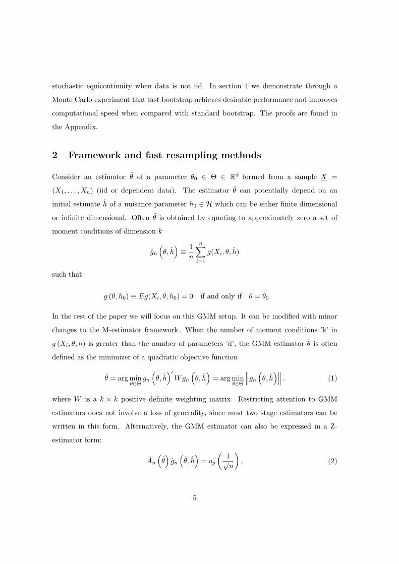
2 Framework and fast resampling methods

Consider an estimator θ of a parameter θ0 ∈ Θ ∈ Rd formed from a sample X =

(X1, . . . , Xn) (iid or dependent data). The estimator θ can potentially depend on an

initial estimate h of a nuisance parameter h0 ∈ H which can be either finite dimensional

or infinite dimensional. Often θ is obtained by equating to approximately zero a set of

moment conditions of dimension k

gn

(

θ, h)

≡ 1

n

n∑

i=1

g(Xi, θ, h)

such that

g (θ, h0) ≡ Eg(Xi, θ, h0) = 0 if and only if θ = θ0.

In the rest of the paper we will focus on this GMM setup. It can be modified with minor

changes to the M-estimator framework. When the number of moment conditions ’k’ in

g (Xi, θ, h) is greater than the number of parameters ’d’, the GMM estimator θ is often

defined as the minimizer of a quadratic objective function

θ = argminθ∈Θ

gn

(

θ, h)′Wgn

(

θ, h)

= argminθ∈Θ

∥

∥

∥gn

(

θ, h)∥

∥

∥. (1)

where W is a k × k positive definite weighting matrix. Restricting attention to GMM

estimators does not involve a loss of generality, since most two stage estimators can be

written in this form. Alternatively, the GMM estimator can also be expressed in a Z-

estimator form:

An

(

θ)

gn

(

θ, h)

= op

(

1√n

)

, (2)

5

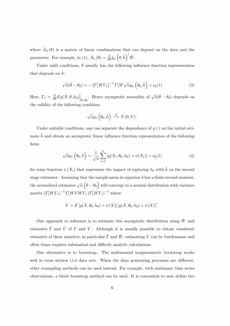
where An (θ) is a matrix of linear combinations that can depend on the data and the

parameter. For example, in (1), An (θ) =∂∂θ gn

(

θ, h)′W .

Under mild conditions, θ usually has the following influence function representation

that depends on h:

√n(θ − θ0) = −

(

Γ′1WΓ1

)−1Γ′1W

√ngn

(

θ0, h)

+ op(1) (3)

Here, Γ1 = ∂∂θEg(X, θ, h0)

∣

∣

∣

θ=θ0. Hence asymptotic normality of

√n(θ − θ0) depends on

the validity of the following condition:

√ngn

(

θ0, h)

d−→ N (0, V ) .

Under suitable conditions, one can separate the dependence of g (·) on the initial esti-

mate h and obtain an asymptotic linear influence function representation of the following

form:

√ngn

(

θ0, h)

=1√n

n∑

i=1

[g(Xi, θ0, h0) + ψ(Xi)] + op(1) (4)

for some function ψ (Xi) that represents the impact of replacing h0 with h on the second

stage estimator. Assuming that the sample mean in equation 4 has a finite second moment,

the normalized estimator√n(

θ − θ0

)

will converge to a normal distribution with variance

matrix (Γ′1WΓ1)

−1 Γ′1WVWΓ1 (Γ

′1WΓ1)

−1 where

V = E [g(X, θ0, h0) + ψ(X)] [g(X, θ0, h0) + ψ(X)]′ .

One approach to inference is to estimate this asymptotic distribution using W and

estimates Γ and V of Γ and V . Although it is usually possible to obtain consistent

estimates of these matrices, in particular Γ and W , estimating V can be burdensome and

often times requires substantial and difficult analytic calculations.

One alternative is to bootstrap. The multinomial nonparametric bootstrap works

well in cross section i.i.d data sets. When the data generating processes are different,

other resampling methods can be used instead. For example, with stationary time series

observations, a block bootstrap method can be used. It is convenient to now define two

6

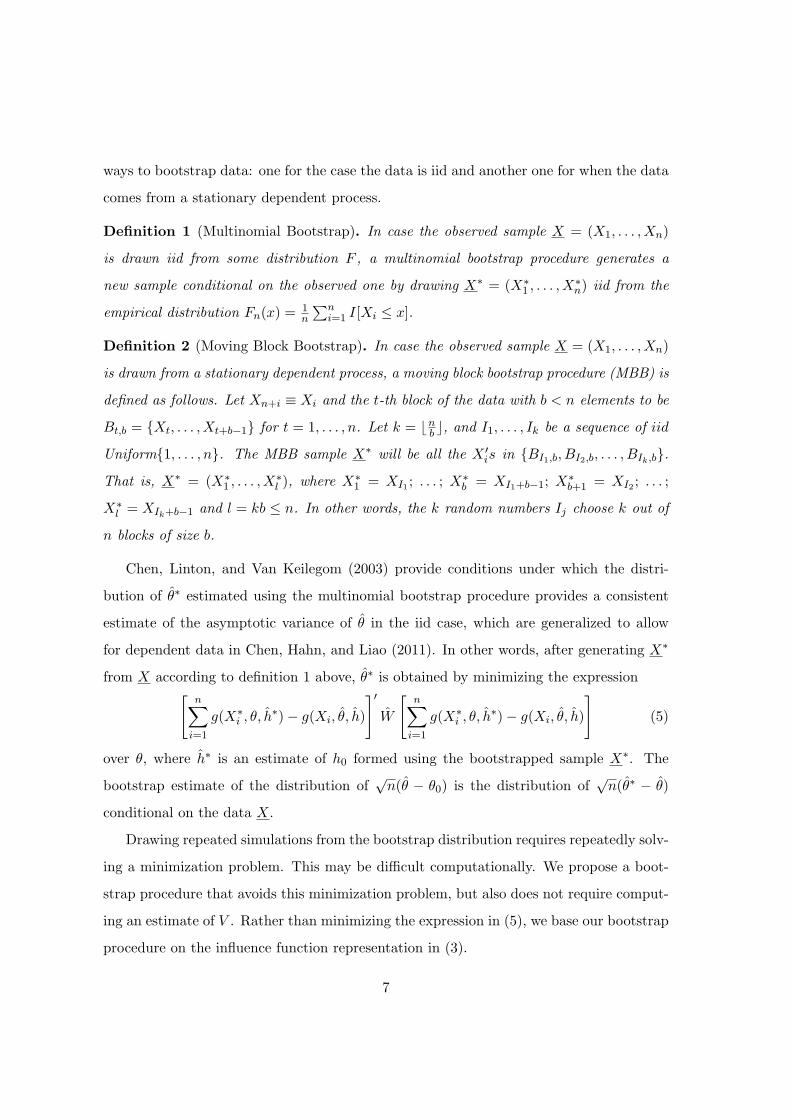
ways to bootstrap data: one for the case the data is iid and another one for when the data

comes from a stationary dependent process.

Definition 1 (Multinomial Bootstrap). In case the observed sample X = (X1, . . . , Xn)

is drawn iid from some distribution F , a multinomial bootstrap procedure generates a

new sample conditional on the observed one by drawing X∗ = (X∗1 , . . . , X

∗n) iid from the

empirical distribution Fn(x) =1n

∑ni=1 I[Xi ≤ x].

Definition 2 (Moving Block Bootstrap). In case the observed sample X = (X1, . . . , Xn)

is drawn from a stationary dependent process, a moving block bootstrap procedure (MBB) is

defined as follows. Let Xn+i ≡ Xi and the t-th block of the data with b < n elements to be

Bt,b = Xt, . . . , Xt+b−1 for t = 1, . . . , n. Let k = ⌊nb ⌋, and I1, . . . , Ik be a sequence of iid

Uniform1, . . . , n. The MBB sample X∗ will be all the X ′is in BI1,b, BI2,b, . . . , BIk,b.

That is, X∗ = (X∗1 , . . . , X

∗l ), where X∗

1 = XI1 ; . . . ; X∗b = XI1+b−1; X

∗b+1 = XI2 ; . . . ;

X∗l = XIk+b−1 and l = kb ≤ n. In other words, the k random numbers Ij choose k out of

n blocks of size b.

Chen, Linton, and Van Keilegom (2003) provide conditions under which the distri-

bution of θ∗ estimated using the multinomial bootstrap procedure provides a consistent

estimate of the asymptotic variance of θ in the iid case, which are generalized to allow

for dependent data in Chen, Hahn, and Liao (2011). In other words, after generating X∗

from X according to definition 1 above, θ∗ is obtained by minimizing the expression[

n∑

i=1

g(X∗i , θ, h

∗)− g(Xi, θ, h)

]′

W

[

n∑

i=1

g(X∗i , θ, h

∗)− g(Xi, θ, h)

]

(5)

over θ, where h∗ is an estimate of h0 formed using the bootstrapped sample X∗. The

bootstrap estimate of the distribution of√n(θ − θ0) is the distribution of

√n(θ∗ − θ)

conditional on the data X.

Drawing repeated simulations from the bootstrap distribution requires repeatedly solv-

ing a minimization problem. This may be difficult computationally. We propose a boot-

strap procedure that avoids this minimization problem, but also does not require comput-

ing an estimate of V . Rather than minimizing the expression in (5), we base our bootstrap

procedure on the influence function representation in (3).

7

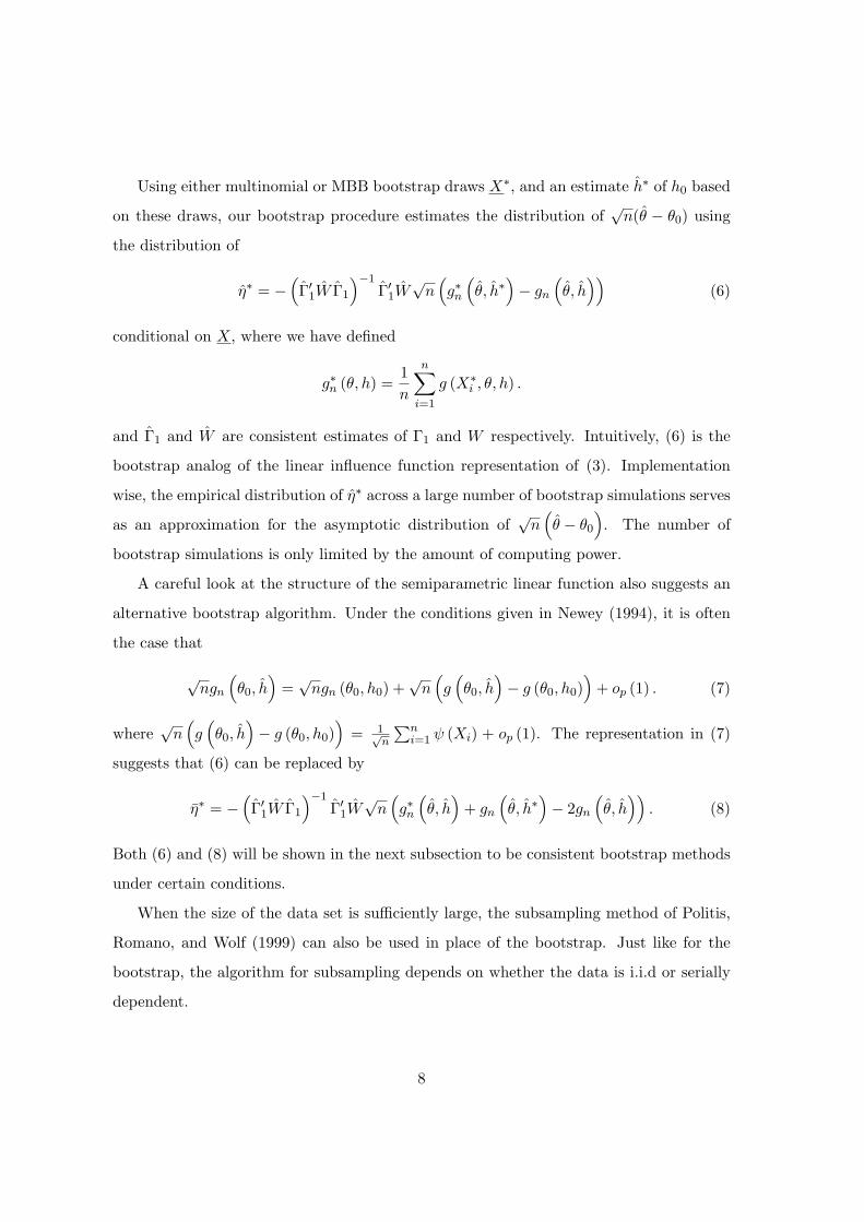
Using either multinomial or MBB bootstrap draws X∗, and an estimate h∗ of h0 based

on these draws, our bootstrap procedure estimates the distribution of√n(θ − θ0) using

the distribution of

η∗ = −(

Γ′1W Γ1

)−1Γ′1W

√n(

g∗n(

θ, h∗)

− gn

(

θ, h))

(6)

conditional on X, where we have defined

g∗n (θ, h) =1

n

n∑

i=1

g (X∗i , θ, h) .

and Γ1 and W are consistent estimates of Γ1 and W respectively. Intuitively, (6) is the

bootstrap analog of the linear influence function representation of (3). Implementation

wise, the empirical distribution of η∗ across a large number of bootstrap simulations serves

as an approximation for the asymptotic distribution of√n(

θ − θ0

)

. The number of

bootstrap simulations is only limited by the amount of computing power.

A careful look at the structure of the semiparametric linear function also suggests an

alternative bootstrap algorithm. Under the conditions given in Newey (1994), it is often

the case that

√ngn

(

θ0, h)

=√ngn (θ0, h0) +

√n(

g(

θ0, h)

− g (θ0, h0))

+ op (1) . (7)

where√n(

g(

θ0, h)

− g (θ0, h0))

= 1√n

∑ni=1 ψ (Xi) + op (1). The representation in (7)

suggests that (6) can be replaced by

η∗ = −(

Γ′1W Γ1

)−1Γ′1W

√n(

g∗n(

θ, h)

+ gn

(

θ, h∗)

− 2gn

(

θ, h))

. (8)

Both (6) and (8) will be shown in the next subsection to be consistent bootstrap methods

under certain conditions.

When the size of the data set is sufficiently large, the subsampling method of Politis,

Romano, and Wolf (1999) can also be used in place of the bootstrap. Just like for the

bootstrap, the algorithm for subsampling depends on whether the data is i.i.d or serially

dependent.

8

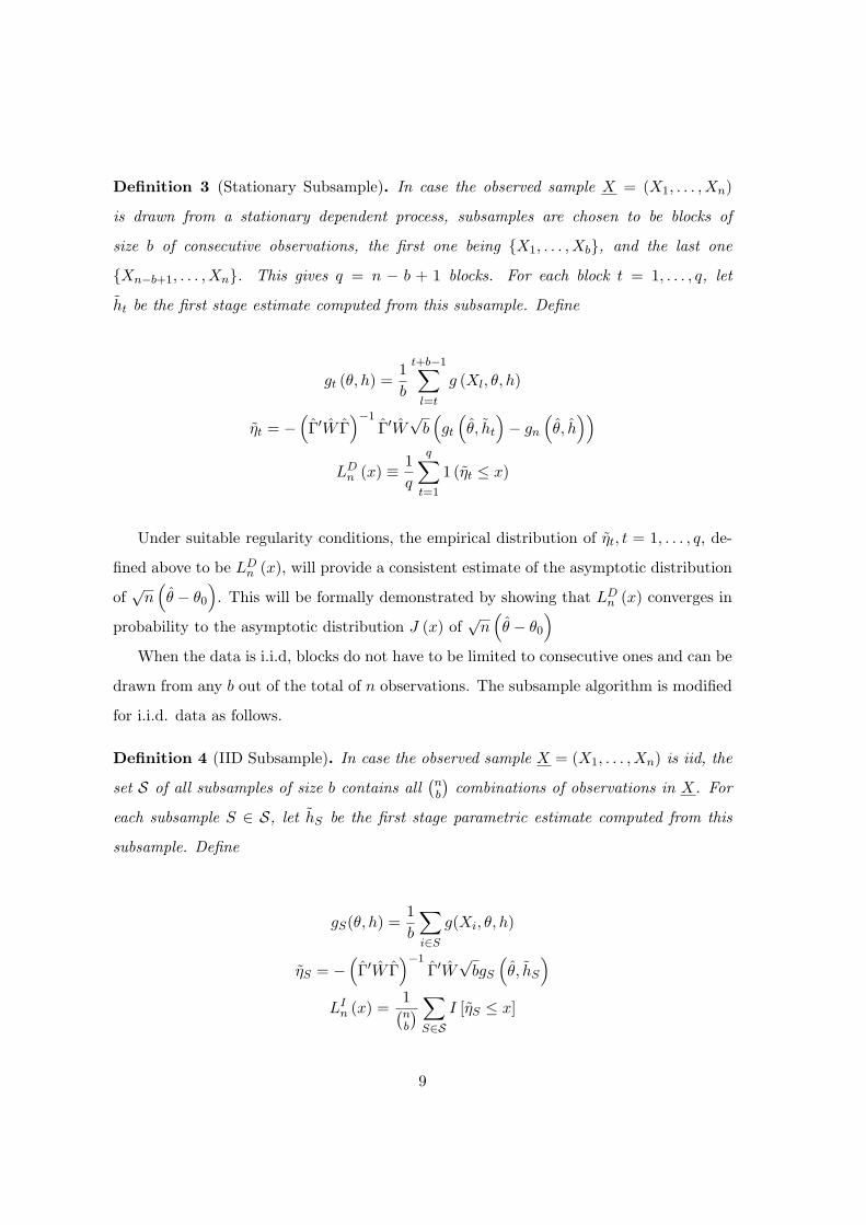
Definition 3 (Stationary Subsample). In case the observed sample X = (X1, . . . , Xn)

is drawn from a stationary dependent process, subsamples are chosen to be blocks of

size b of consecutive observations, the first one being X1, . . . , Xb, and the last one

Xn−b+1, . . . , Xn. This gives q = n − b + 1 blocks. For each block t = 1, . . . , q, let

ht be the first stage estimate computed from this subsample. Define

gt (θ, h) =1

b

t+b−1∑

l=t

g (Xl, θ, h)

ηt = −(

Γ′W Γ)−1

Γ′W√b(

gt

(

θ, ht

)

− gn

(

θ, h))

LDn (x) ≡ 1

q

q∑

t=1

1 (ηt ≤ x)

Under suitable regularity conditions, the empirical distribution of ηt, t = 1, . . . , q, de-

fined above to be LDn (x), will provide a consistent estimate of the asymptotic distribution

of√n(

θ − θ0

)

. This will be formally demonstrated by showing that LDn (x) converges in

probability to the asymptotic distribution J (x) of√n(

θ − θ0

)

When the data is i.i.d, blocks do not have to be limited to consecutive ones and can be

drawn from any b out of the total of n observations. The subsample algorithm is modified

for i.i.d. data as follows.

Definition 4 (IID Subsample). In case the observed sample X = (X1, . . . , Xn) is iid, the

set S of all subsamples of size b contains all(

nb

)

combinations of observations in X. For

each subsample S ∈ S, let hS be the first stage parametric estimate computed from this

subsample. Define

gS(θ, h) =1

b

∑

i∈Sg(Xi, θ, h)

ηS = −(

Γ′W Γ)−1

Γ′W√bgS

(

θ, hS

)

LIn (x) =

1(

nb

)

∑

S∈SI [ηS ≤ x]

9

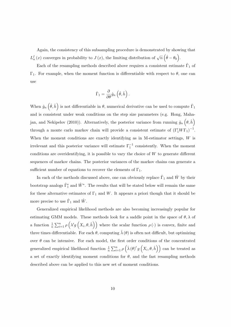
Again, the consistency of this subsampling procedure is demonstrated by showing that

LIn (x) converges in probability to J (x), the limiting distribution of

√n(

θ − θ0

)

.

Each of the resampling methods described above requires a consistent estimate Γ1 of

Γ1. For example, when the moment function is differentiable with respect to θ, one can

use

Γ1 =∂

∂θgn

(

θ, h)

.

When gn

(

θ, h)

is not differentiable in θ, numerical derivative can be used to compute Γ1

and is consistent under weak conditions on the step size parameters (e.g. Hong, Maha-

jan, and Nekipelov (2010)). Alternatively, the posterior variance from running gn

(

θ, h)

through a monte carlo markov chain will provide a consistent estimate of (Γ′1WΓ1)

−1.

When the moment conditions are exactly identifying as in M-estimator settings, W is

irrelevant and this posterior variance will estimate Γ−11 consistently. When the moment

conditions are overidentifying, it is possible to vary the choice of W to generate different

sequences of markov chains. The posterior variances of the markov chains can generate a

sufficient number of equations to recover the elements of Γ1.

In each of the methods discussed above, one can obviously replace Γ1 and W by their

bootstrap analogs Γ∗1 and W ∗. The results that will be stated below will remain the same

for these alternative estimates of Γ1 and W . It appears a priori though that it should be

more precise to use Γ1 and W .

Generalized empirical likelihood methods are also becoming increasingly popular for

estimating GMM models. These methods look for a saddle point in the space of θ, λ of

a function 1n

∑ni=1 ρ

(

λ′g(

Xi, θ, h))

where the scalar function ρ (·) is convex, finite and

three times differentiable. For each θ, computing λ (θ) is often not difficult, but optimizing

over θ can be intensive. For each model, the first order conditions of the concentrated

generalized empirical likelihood function 1n

∑ni=1 ρ

(

λ (θ)′ g(

Xi, θ, h))

can be treated as

a set of exactly identifying moment conditions for θ, and the fast resampling methods

described above can be applied to this new set of moment conditions.

10

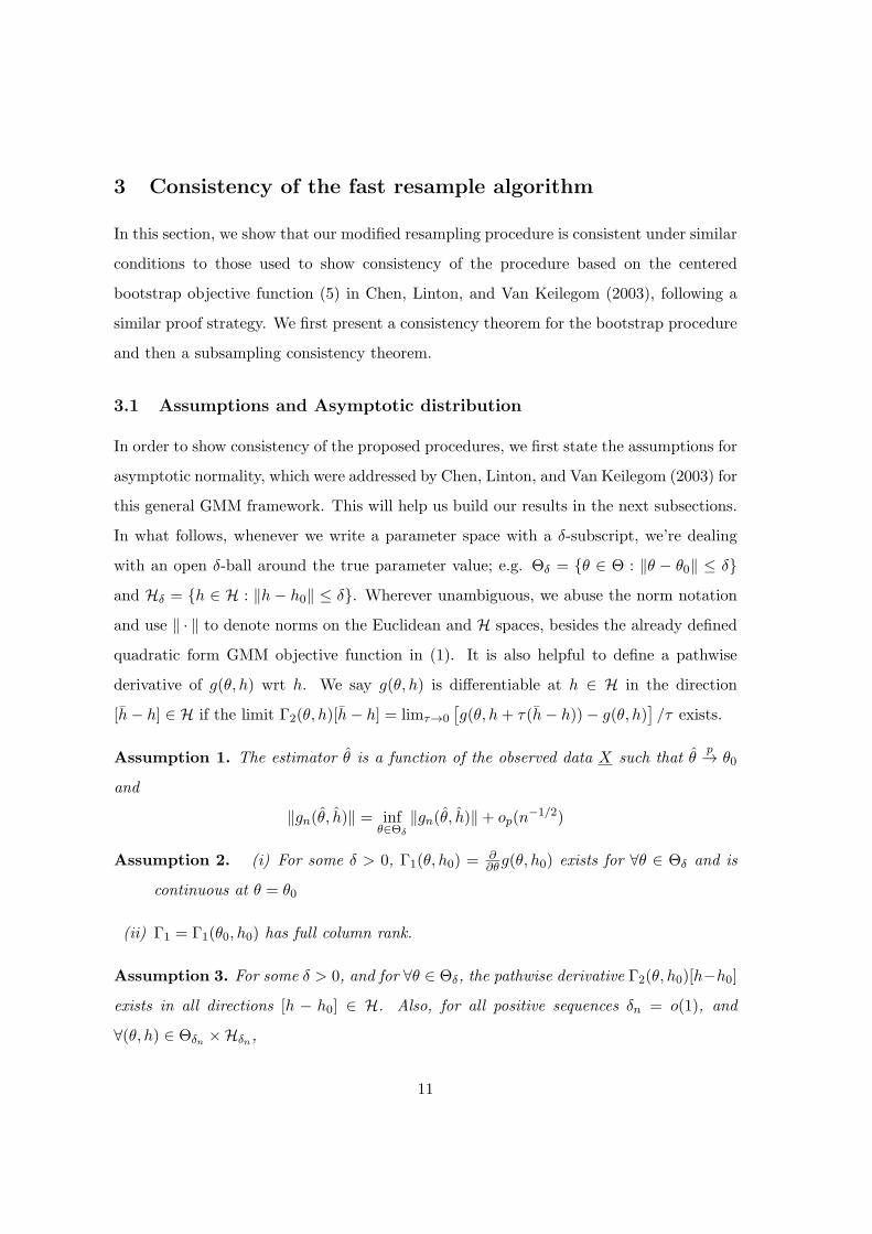
3 Consistency of the fast resample algorithm

In this section, we show that our modified resampling procedure is consistent under similar

conditions to those used to show consistency of the procedure based on the centered

bootstrap objective function (5) in Chen, Linton, and Van Keilegom (2003), following a

similar proof strategy. We first present a consistency theorem for the bootstrap procedure

and then a subsampling consistency theorem.

3.1 Assumptions and Asymptotic distribution

In order to show consistency of the proposed procedures, we first state the assumptions for

asymptotic normality, which were addressed by Chen, Linton, and Van Keilegom (2003) for

this general GMM framework. This will help us build our results in the next subsections.

In what follows, whenever we write a parameter space with a δ-subscript, we’re dealing

with an open δ-ball around the true parameter value; e.g. Θδ = θ ∈ Θ : ‖θ − θ0‖ ≤ δand Hδ = h ∈ H : ‖h − h0‖ ≤ δ. Wherever unambiguous, we abuse the norm notation

and use ‖ · ‖ to denote norms on the Euclidean and H spaces, besides the already defined

quadratic form GMM objective function in (1). It is also helpful to define a pathwise

derivative of g(θ, h) wrt h. We say g(θ, h) is differentiable at h ∈ H in the direction

[h− h] ∈ H if the limit Γ2(θ, h)[h− h] = limτ→0

[

g(θ, h+ τ(h− h))− g(θ, h)]

/τ exists.

Assumption 1. The estimator θ is a function of the observed data X such that θp→ θ0

and

‖gn(θ, h)‖ = infθ∈Θδ

‖gn(θ, h)‖+ op(n−1/2)

Assumption 2. (i) For some δ > 0, Γ1(θ, h0) =∂∂θg(θ, h0) exists for ∀θ ∈ Θδ and is

continuous at θ = θ0

(ii) Γ1 = Γ1(θ0, h0) has full column rank.

Assumption 3. For some δ > 0, and for ∀θ ∈ Θδ, the pathwise derivative Γ2(θ, h0)[h−h0]exists in all directions [h − h0] ∈ H. Also, for all positive sequences δn = o(1), and

∀(θ, h) ∈ Θδn ×Hδn,

11

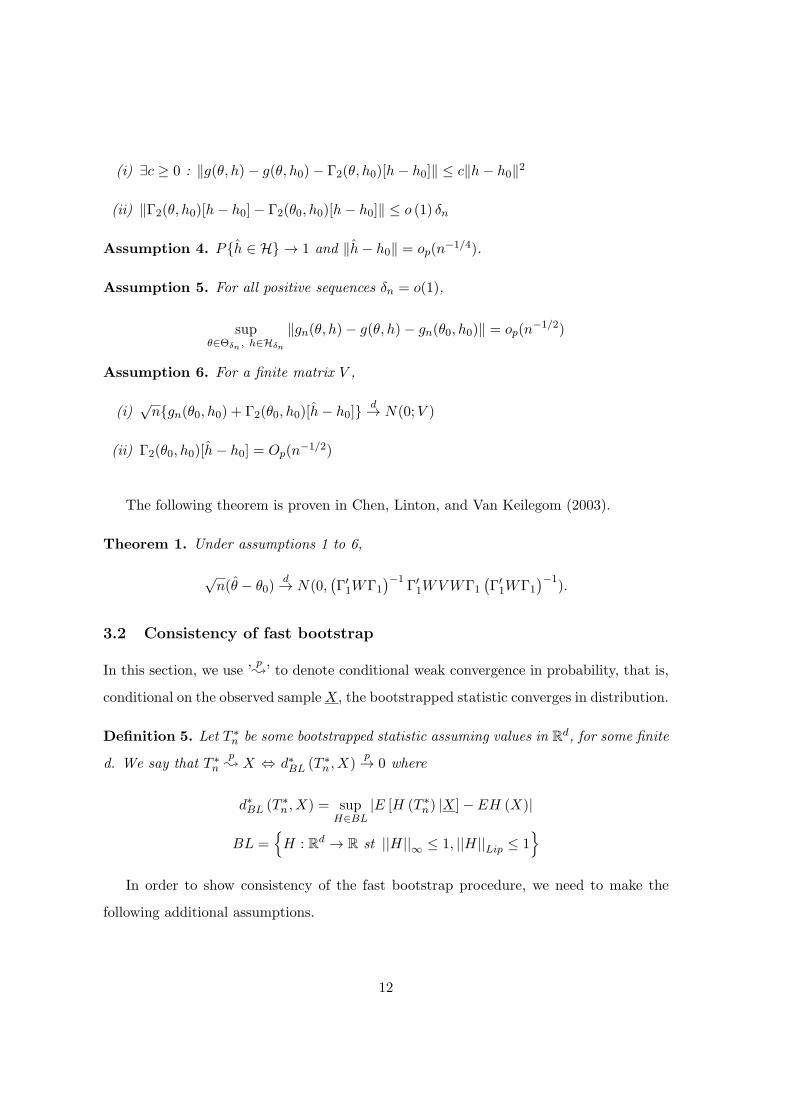
(i) ∃c ≥ 0 : ‖g(θ, h)− g(θ, h0)− Γ2(θ, h0)[h− h0]‖ ≤ c‖h− h0‖2

(ii) ‖Γ2(θ, h0)[h− h0]− Γ2(θ0, h0)[h− h0]‖ ≤ o (1) δn

Assumption 4. Ph ∈ H → 1 and ‖h− h0‖ = op(n−1/4).

Assumption 5. For all positive sequences δn = o(1),

supθ∈Θδn , h∈Hδn

‖gn(θ, h)− g(θ, h)− gn(θ0, h0)‖ = op(n−1/2)

Assumption 6. For a finite matrix V ,

(i)√ngn(θ0, h0) + Γ2(θ0, h0)[h− h0] d→ N(0;V )

(ii) Γ2(θ0, h0)[h− h0] = Op(n−1/2)

The following theorem is proven in Chen, Linton, and Van Keilegom (2003).

Theorem 1. Under assumptions 1 to 6,

√n(θ − θ0)

d→ N(0,(

Γ′1WΓ1

)−1Γ′1WVWΓ1

(

Γ′1WΓ1

)−1).

3.2 Consistency of fast bootstrap

In this section, we use ’p;’ to denote conditional weak convergence in probability, that is,

conditional on the observed sampleX, the bootstrapped statistic converges in distribution.

Definition 5. Let T ∗n be some bootstrapped statistic assuming values in R

d, for some finite

d. We say that T ∗n

p; X ⇔ d∗BL (T ∗

n , X)p→ 0 where

d∗BL (T ∗n , X) = sup

H∈BL|E [H (T ∗

n) |X]− EH (X)|

BL =

H : Rd → R st ||H||∞ ≤ 1, ||H||Lip ≤ 1

In order to show consistency of the fast bootstrap procedure, we need to make the

following additional assumptions.

12

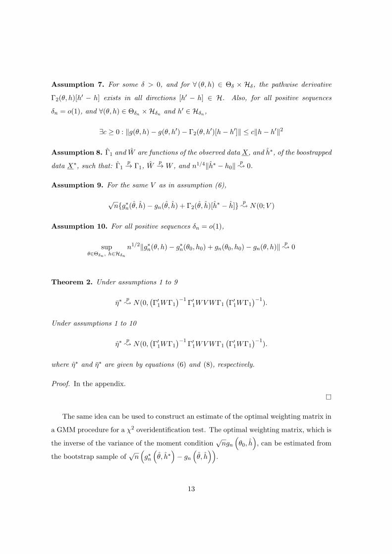
Assumption 7. For some δ > 0, and for ∀ (θ, h) ∈ Θδ × Hδ, the pathwise derivative

Γ2(θ, h)[h′ − h] exists in all directions [h′ − h] ∈ H. Also, for all positive sequences

δn = o(1), and ∀(θ, h) ∈ Θδn ×Hδn and h′ ∈ Hδn,

∃c ≥ 0 : ‖g(θ, h)− g(θ, h′)− Γ2(θ, h′)[h− h′]‖ ≤ c‖h− h′‖2

Assumption 8. Γ1 and W are functions of the observed data X, and h∗, of the boostrapped

data X∗, such that: Γ1p→ Γ1, W

p→W , and n1/4‖h∗ − h0‖p; 0.

Assumption 9. For the same V as in assumption (6),

√ng∗n(θ, h)− gn(θ, h) + Γ2(θ, h)[h

∗ − h] p; N(0;V )

Assumption 10. For all positive sequences δn = o(1),

supθ∈Θδn , h∈Hδn

n1/2‖g∗n(θ, h)− g∗n(θ0, h0) + gn(θ0, h0)− gn(θ, h)‖p; 0

Theorem 2. Under assumptions 1 to 9

η∗p; N(0,

(

Γ′1WΓ1

)−1Γ′1WVWΓ1

(

Γ′1WΓ1

)−1).

Under assumptions 1 to 10

η∗p; N(0,

(

Γ′1WΓ1

)−1Γ′1WVWΓ1

(

Γ′1WΓ1

)−1).

where η∗ and η∗ are given by equations (6) and (8), respectively.

Proof. In the appendix.

The same idea can be used to construct an estimate of the optimal weighting matrix in

a GMM procedure for a χ2 overidentification test. The optimal weighting matrix, which is

the inverse of the variance of the moment condition√ngn

(

θ0, h)

, can be estimated from

the bootstrap sample of√n(

g∗n(

θ, h∗)

− gn

(

θ, h))

.

13

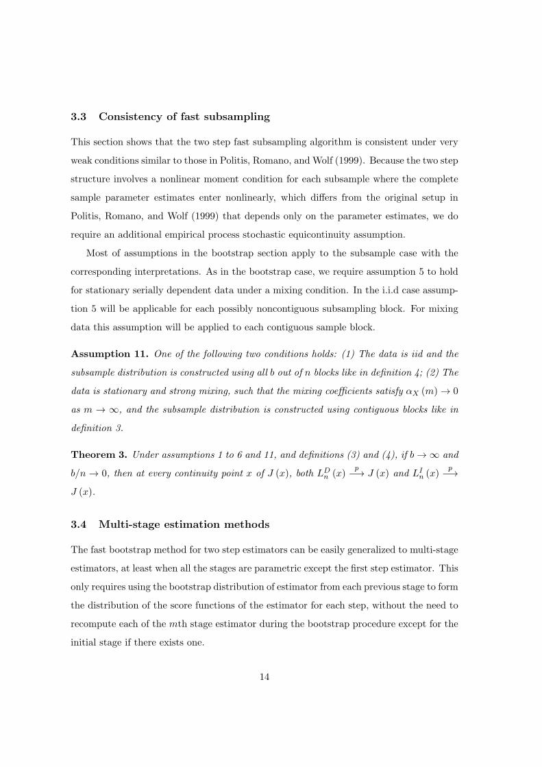
3.3 Consistency of fast subsampling

This section shows that the two step fast subsampling algorithm is consistent under very

weak conditions similar to those in Politis, Romano, and Wolf (1999). Because the two step

structure involves a nonlinear moment condition for each subsample where the complete

sample parameter estimates enter nonlinearly, which differs from the original setup in

Politis, Romano, and Wolf (1999) that depends only on the parameter estimates, we do

require an additional empirical process stochastic equicontinuity assumption.

Most of assumptions in the bootstrap section apply to the subsample case with the

corresponding interpretations. As in the bootstrap case, we require assumption 5 to hold

for stationary serially dependent data under a mixing condition. In the i.i.d case assump-

tion 5 will be applicable for each possibly noncontiguous subsampling block. For mixing

data this assumption will be applied to each contiguous sample block.

Assumption 11. One of the following two conditions holds: (1) The data is iid and the

subsample distribution is constructed using all b out of n blocks like in definition 4; (2) The

data is stationary and strong mixing, such that the mixing coefficients satisfy αX (m) → 0

as m → ∞, and the subsample distribution is constructed using contiguous blocks like in

definition 3.

Theorem 3. Under assumptions 1 to 6 and 11, and definitions (3) and (4), if b→ ∞ and

b/n → 0, then at every continuity point x of J (x), both LDn (x)

p−→ J (x) and LIn (x)

p−→J (x).

3.4 Multi-stage estimation methods

The fast bootstrap method for two step estimators can be easily generalized to multi-stage

estimators, at least when all the stages are parametric except the first step estimator. This

only requires using the bootstrap distribution of estimator from each previous stage to form

the distribution of the score functions of the estimator for each step, without the need to

recompute each of the mth stage estimator during the bootstrap procedure except for the

initial stage if there exists one.

14

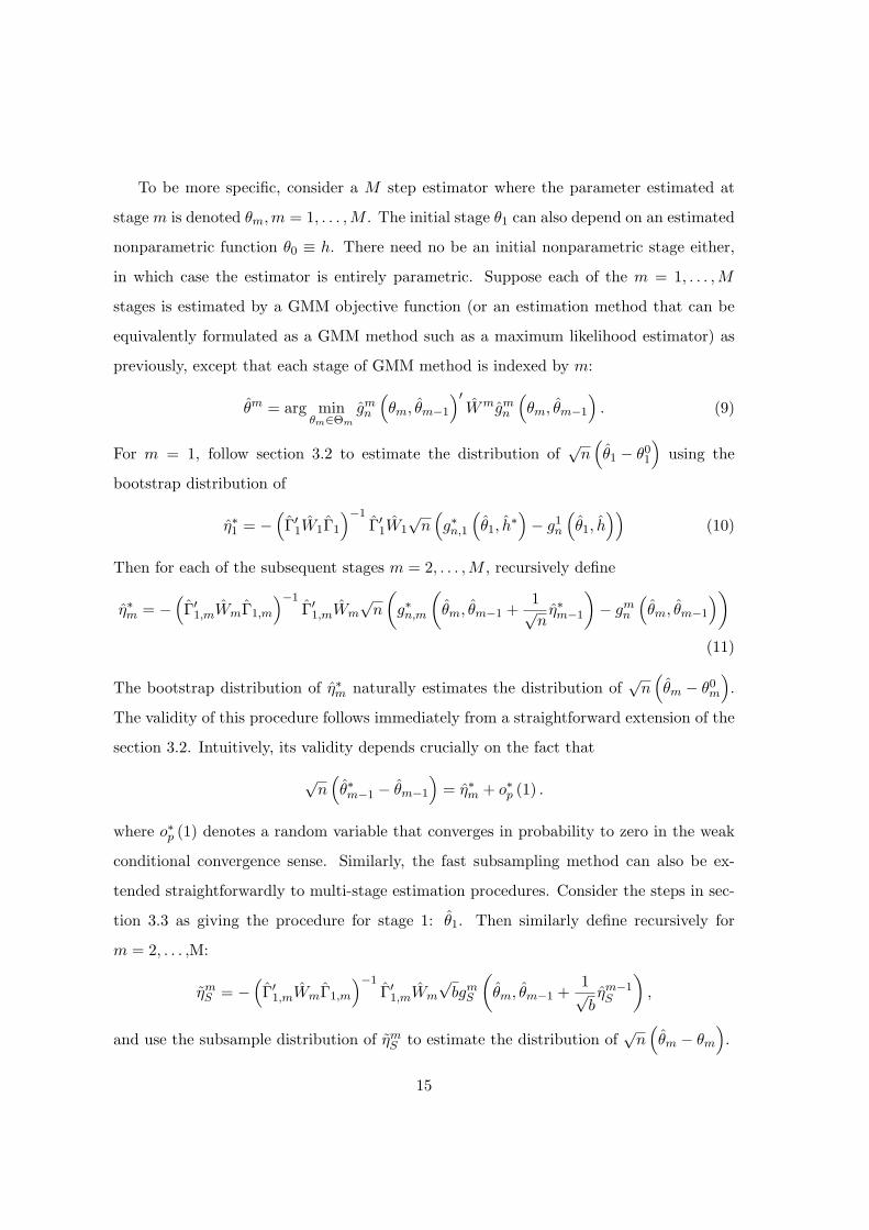
To be more specific, consider a M step estimator where the parameter estimated at

stagem is denoted θm,m = 1, . . . ,M . The initial stage θ1 can also depend on an estimated

nonparametric function θ0 ≡ h. There need no be an initial nonparametric stage either,

in which case the estimator is entirely parametric. Suppose each of the m = 1, . . . ,M

stages is estimated by a GMM objective function (or an estimation method that can be

equivalently formulated as a GMM method such as a maximum likelihood estimator) as

previously, except that each stage of GMM method is indexed by m:

θm = arg minθm∈Θm

gmn

(

θm, θm−1

)′Wmgmn

(

θm, θm−1

)

. (9)

For m = 1, follow section 3.2 to estimate the distribution of√n(

θ1 − θ01

)

using the

bootstrap distribution of

η∗1 = −(

Γ′1W1Γ1

)−1Γ′1W1

√n(

g∗n,1(

θ1, h∗)

− g1n

(

θ1, h))

(10)

Then for each of the subsequent stages m = 2, . . . ,M , recursively define

η∗m = −(

Γ′1,mWmΓ1,m

)−1Γ′1,mWm

√n

(

g∗n,m

(

θm, θm−1 +1√nη∗m−1

)

− gmn

(

θm, θm−1

)

)

(11)

The bootstrap distribution of η∗m naturally estimates the distribution of√n(

θm − θ0m

)

.

The validity of this procedure follows immediately from a straightforward extension of the

section 3.2. Intuitively, its validity depends crucially on the fact that

√n(

θ∗m−1 − θm−1

)

= η∗m + o∗p (1) .

where o∗p (1) denotes a random variable that converges in probability to zero in the weak

conditional convergence sense. Similarly, the fast subsampling method can also be ex-

tended straightforwardly to multi-stage estimation procedures. Consider the steps in sec-

tion 3.3 as giving the procedure for stage 1: θ1. Then similarly define recursively for

m = 2, . . . ,M:

ηmS = −(

Γ′1,mWmΓ1,m

)−1Γ′1,mWm

√bgmS

(

θm, θm−1 +1√bηm−1S

)

,

and use the subsample distribution of ηmS to estimate the distribution of√n(

θm − θm

)

.

15

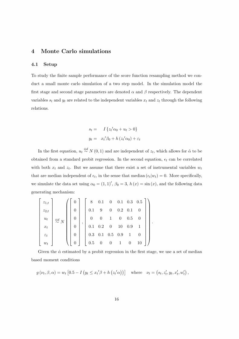
4 Monte Carlo simulations

4.1 Setup

To study the finite sample performance of the score function resampling method we con-

duct a small monte carlo simulation of a two step model. In the simulation model the

first stage and second stage parameters are denoted α and β respectively. The dependent

variables st and yt are related to the independent variables xt and zt through the following

relations.

st = I zt′α0 + ut > 0

yt = xt′β0 + h (zt

′α0) + εt

In the first equation, utiid∼ N (0, 1) and are independent of zt, which allows for α to be

obtained from a standard probit regression. In the second equation, ǫt can be correlated

with both xt and zt. But we assume that there exist a set of instrumental variables wt

that are median independent of ǫt, in the sense that median (ǫt|wt) = 0. More specifically,

we simulate the data set using α0 = (1, 1)′, β0 = 3, h (x) = sin (x), and the following data

generating mechanism:

z1,t

z2,t

ut

xt

εt

wt

iid∼ N

0

0

0

0

0

0

,

8 0.1 0 0.1 0.3 0.5

0.1 9 0 0.2 0.1 0

0 0 1 0 0.5 0

0.1 0.2 0 10 0.9 1

0.3 0.1 0.5 0.9 1 0

0.5 0 0 1 0 10

.

Given the α estimated by a probit regression in the first stage, we use a set of median

based moment conditions

g (νt, β, α) = wt

[

0.5− I(

yt ≤ xt′β + h

(

zt′α))]

where νt =(

st, z′t, yt, x

′t, w

′t

)

,

16

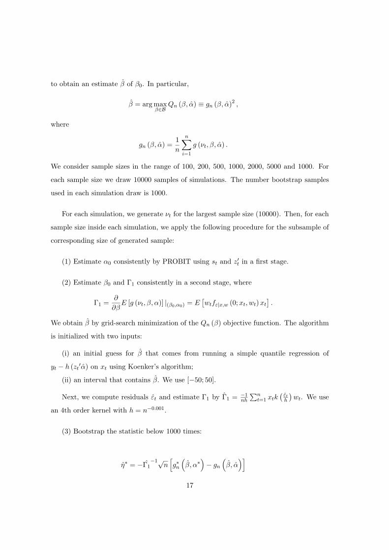
to obtain an estimate β of β0. In particular,

β = argmaxβ∈B

Qn (β, α) ≡ gn (β, α)2 ,

where

gn (β, α) =1

n

n∑

i=1

g (νt, β, α) .

We consider sample sizes in the range of 100, 200, 500, 1000, 2000, 5000 and 1000. For

each sample size we draw 10000 samples of simulations. The number bootstrap samples

used in each simulation draw is 1000.

For each simulation, we generate νt for the largest sample size (10000). Then, for each

sample size inside each simulation, we apply the following procedure for the subsample of

corresponding size of generated sample:

(1) Estimate α0 consistently by PROBIT using st and z′t in a first stage.

(2) Estimate β0 and Γ1 consistently in a second stage, where

Γ1 =∂

∂βE [g (νt, β, α)] |(β0,α0) = E

[

wtfε|x,w (0;xt, wt)xt]

.

We obtain β by grid-search minimization of the Qn (β) objective function. The algorithm

is initialized with two inputs:

(i) an initial guess for β that comes from running a simple quantile regression of

yt − h (zt′α) on xt using Koenker’s algorithm;

(ii) an interval that contains β. We use [−50; 50].

Next, we compute residuals εt and estimate Γ1 by Γ1 = −1nh

∑nt=1 xtk

(

εth

)

wt. We use

an 4th order kernel with h = n−0.001.

(3) Bootstrap the statistic below 1000 times:

η∗ = −Γ1−1√

n[

g∗n(

β, α∗)

− gn

(

β, α)]

17

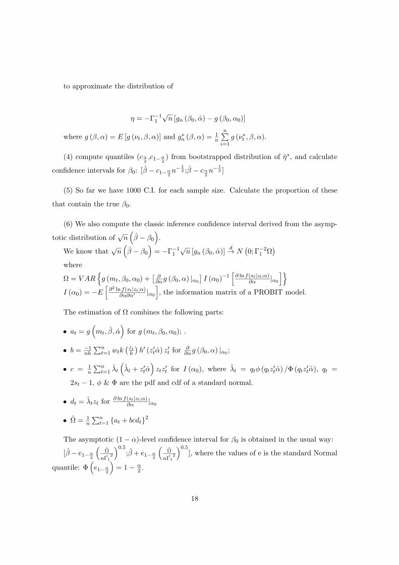
to approximate the distribution of

η = −Γ−11

√n [gn (β0, α)− g (β0, α0)]

where g (β, α) = E [g (νt, β, α)] and g∗n (β, α) =

1n

n∑

i=1g (ν∗t , β, α).

(4) compute quantiles (cα2

,c1−α2

) from bootstrapped distribution of η∗, and calculate

confidence intervals for β0: [β − c1−α2

n−1

2 ;β − cα2

n−1

2 ]

(5) So far we have 1000 C.I. for each sample size. Calculate the proportion of these

that contain the true β0.

(6) We also compute the classic inference confidence interval derived from the asymp-

totic distribution of√n(

β − β0

)

.

We know that√n(

β − β0

)

= −Γ−11

√n [gn (β0, α)]

d→ N(

0; Γ−21 Ω

)

where

Ω = V AR

g (mt, β0, α0) +[

∂∂αg (β0, α) |α0

]

I (α0)−1[

∂ ln f(st|zt;α)∂α |α0

]

I (α0) = −E[

∂2 ln f(st|zt;α)∂α∂α′ |α0

]

, the information matrix of a PROBIT model.

The estimation of Ω combines the following parts:

• at = g(

mt, β, α)

for g (mt, β0, α0); .

• b = −1nh

∑nt=1wtk

(

εth

)

h′ (z′tα) z′t for

∂∂αg (β0, α) |α0

;

• c = 1n

∑nt=1 λt

(

λt + z′tα)

ztz′t for I (α0), where λt = qtφ (qtz

′tα) /Φ (qtz

′tα), qt =

2st − 1, φ & Φ are the pdf and cdf of a standard normal.

• dt = λtzt for∂ ln f(st|zt;α)

∂α |α0

• Ω = 1n

∑nt=1 at + bcdt2

The asymptotic (1− α)-level confidence interval for β0 is obtained in the usual way:

[β− e1−α2

(

Ω

nΓ1

2

)0.5;β+ e1−α

2

(

Ω

nΓ1

2

)0.5], where the values of e is the standard Normal

quantile: Φ(

e1−α2

)

= 1− α2 .

18

4.2 Results

The results from the Monte Carlo simulations are reported in tables 1 to 8 below. Table

1 tabulates the mean, standard deviation and the mean square errors of the sample pa-

rameter estimates across the 1000 simulation draws. As the sample increases, both the

standard deviations and the mean square errors decrease monotonically to zero, assuring

that the sample parameter estimates are consistent. Table 2 reports similar statistics for

the properly normalized and centered estimates that admit a normal limiting distribution.

As predicted by the asymptotic distribution theory, the standard deviations and mean

square errors stabilize for large sample sizes, although β appears to be more difficult to

estimate than α1 and α2.

Tables 3 and 4 report the performance of estimates formed by averaging over the

bootstrap simulations, respectively for the fast bootstrap method and for the conven-

tional bootstrap method. These estimates theoretically should have larger biases than the

original sample estimates.

Tables 5 and 6 report the performance of biased corrected estimates using respectively

the fast bootstrap method and the conventional bootstrap method. These biased corrected

estimates are defined by two times the initial sample estimates minus the averaged boot-

strap estimates. We can see that for the first two parameters α1 and α2, the bias corrected

estimates reported in table 5 have visibly smaller bias than the estimates reported in table

3. However, the benefit of bias reduction is not significant for β. On the other hand,

bias correction tends to increase variation, while taking the average over the bootstrap

sample reduces variation. The net impact of bias reduction on the mean squared error of

the estimates are very small. It seems clear however, that the fast bootstrap bias reduced

estimates outperform the conventional bootstrap bias reduced estimates.

Table 7 reports the empirical coverage probabilities across simulations of the confi-

dence intervals for β0 at three confidence levels, generated according to the fast bootstrap,

the conventional bootstrap and the analytic calculation of the asymptotic distribution.

Both the fast bootstrap confidence interval and the analytic asymptotic confidence in-

terval outperform the conventional bootstrap method in terms of providing more precise

19

coverage of the true parameter β0. This is an interesting result, particularly given that the

conventional bootstrap method is one that is most likely used by empirical researchers.

Finally, table 8 shows the average time in minutes required to run a simulation of this

Monte Carlo exercise, for each sample size and both resampling methods. We can see

that, even for this simple example, the conventional bootstrap method can be quite time

consuming. The fast-bootstrap was about 10 to 20 times faster depending on the sample

size.

[Table 1 about here.]

[Table 2 about here.]

[Table 3 about here.]

[Table 4 about here.]

20

5 Conclusion

We have proposed a fast resampling method. The method directly exploits estimating

(score) functions computed on each resampled draw and avoids recomputing the estimators

for each of them. Fast resampling is easy to perform, and achieves satisfactory performance

while improving considerably numerical speed. These advantages should be of interest for

applied researchers using nonlinear and dynamic models to conduct effective inference.

Our analysis also suggests that while analytical or numerical variance formulas, resam-

pling and MCMC can each be used to obtain valid asymptotic inference, using them in

combination instead of in isolation can offer more powerful tools for computing standard

errors and constructing confidence intervals and test statistics.

References

Ackerberg, D., X. Chen, and J. Hahn (2011): “A Practical Asymptotic Variance

Estimator for Two-Step Semiparametric Estimators,” Cowles Foundation Discussion

Paper No. 1803.

Andrews, D. (1994): “Asymptotics for Semiparametric Econometric Models via Stochas-

tic Equicontinuity,” Econometrica, 62, 43–72.

(2002): “Higher-Order Improvements of a Computationally Attractive k-Step

Bootstrap for Extremum Estimators,” Econometrica, 70(1), 119–162.

Chen, X. (2007): “Large Sample Sieve Estimation of Semi-nonparametric Models,” in

Handbook of Econometrics, Vol 6. Elsevier Science.

Chen, X., J. Hahn, and Z. Liao (2011): “Semiparametric Two-Step GMM with Weakly

Dependent Data,” Working paper, Yale University and UCLA.

Chen, X., O. Linton, and I. Van Keilegom (2003): “Estimation of Semiparametric

Models when the Criterion Function Is Not Smooth,” Econometrica, 71, 1591–1608.

21

Davidson, R., and J. MacKinnon (1999): “Bootstrap Testing in Nonlinear Models,”

International Economic Review, 40, 487–508.

Goncalves, S., and H. White (2004): “Maximum Likelihood and the Bootstrap for

Nonlinear Dynamic Models,” Journal of Econometrics, 119, 199–219.

Hong, H., A. Mahajan, and D. Nekipelov (2010): “Extremum Estimation and Nu-

merical Derivatives,” working paper, UC Berkeley and Stanford University.

Kosorok, M. (2008): Introduction to Empirical Processes and Semiparametric Inference.

Springer Verlag.

Newey, W. (1994): “The Asymptotic Variance of Semiparametric Estimators,” Econo-

metrica, 62, 1349–82.

Pakes, A., and D. Pollard (1989): “Simulation and the Asymptotics of Optimization

Estimators,” Econometrica, 57, 1027–1057.

Politis, D., J. Romano, and M. Wolf (1999): Subsampling. Springer Series in Statis-

tics.

Pollard, D. (1984): Convergence of Stochastic Processes. Springer.

Radulovic, D. (1996): “The Bootstrap for Empirical Processes Based on Stationary

Observations,” Stochastic Processes and their Applications, 65(2), 259–279.

22

6 Appendix

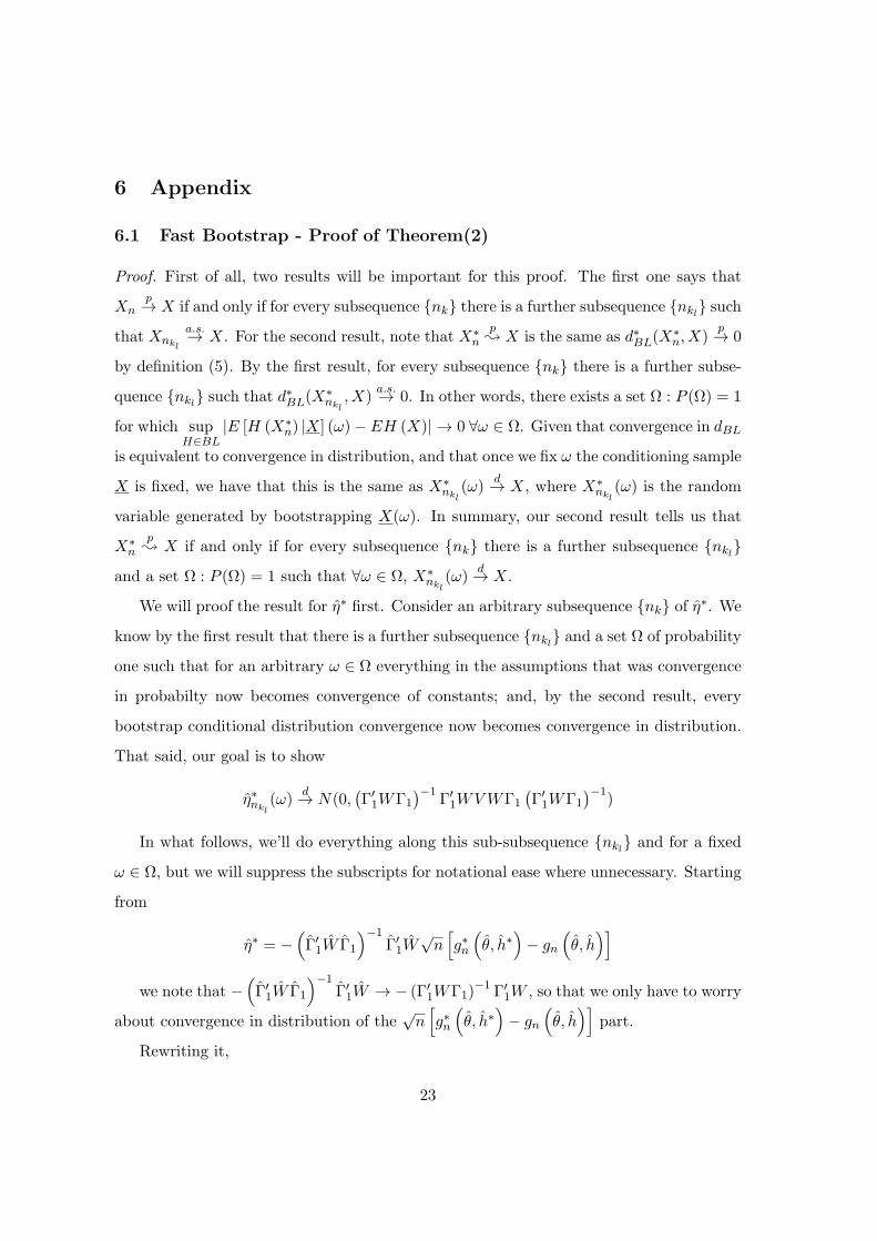
6.1 Fast Bootstrap - Proof of Theorem(2)

Proof. First of all, two results will be important for this proof. The first one says that

Xnp→ X if and only if for every subsequence nk there is a further subsequence nkl such

that Xnkl

a.s.→ X. For the second result, note that X∗n

p; X is the same as d∗BL(X

∗n, X)

p→ 0

by definition (5). By the first result, for every subsequence nk there is a further subse-

quence nkl such that d∗BL(X∗nkl, X)

a.s.→ 0. In other words, there exists a set Ω : P (Ω) = 1

for which supH∈BL

|E [H (X∗n) |X] (ω)− EH (X)| → 0 ∀ω ∈ Ω. Given that convergence in dBL

is equivalent to convergence in distribution, and that once we fix ω the conditioning sample

X is fixed, we have that this is the same as X∗nkl

(ω)d→ X, where X∗

nkl(ω) is the random

variable generated by bootstrapping X(ω). In summary, our second result tells us that

X∗n

p; X if and only if for every subsequence nk there is a further subsequence nkl

and a set Ω : P (Ω) = 1 such that ∀ω ∈ Ω, X∗nkl

(ω)d→ X.

We will proof the result for η∗ first. Consider an arbitrary subsequence nk of η∗. We

know by the first result that there is a further subsequence nkl and a set Ω of probability

one such that for an arbitrary ω ∈ Ω everything in the assumptions that was convergence

in probabilty now becomes convergence of constants; and, by the second result, every

bootstrap conditional distribution convergence now becomes convergence in distribution.

That said, our goal is to show

η∗nkl(ω)

d→ N(0,(

Γ′1WΓ1

)−1Γ′1WVWΓ1

(

Γ′1WΓ1

)−1)

In what follows, we’ll do everything along this sub-subsequence nkl and for a fixed

ω ∈ Ω, but we will suppress the subscripts for notational ease where unnecessary. Starting

from

η∗ = −(

Γ′1W Γ1

)−1Γ′1W

√n[

g∗n(

θ, h∗)

− gn

(

θ, h)]

we note that −(

Γ′1W Γ1

)−1Γ′1W → − (Γ′

1WΓ1)−1 Γ′

1W , so that we only have to worry

about convergence in distribution of the√n[

g∗n(

θ, h∗)

− gn

(

θ, h)]

part.

Rewriting it,

23

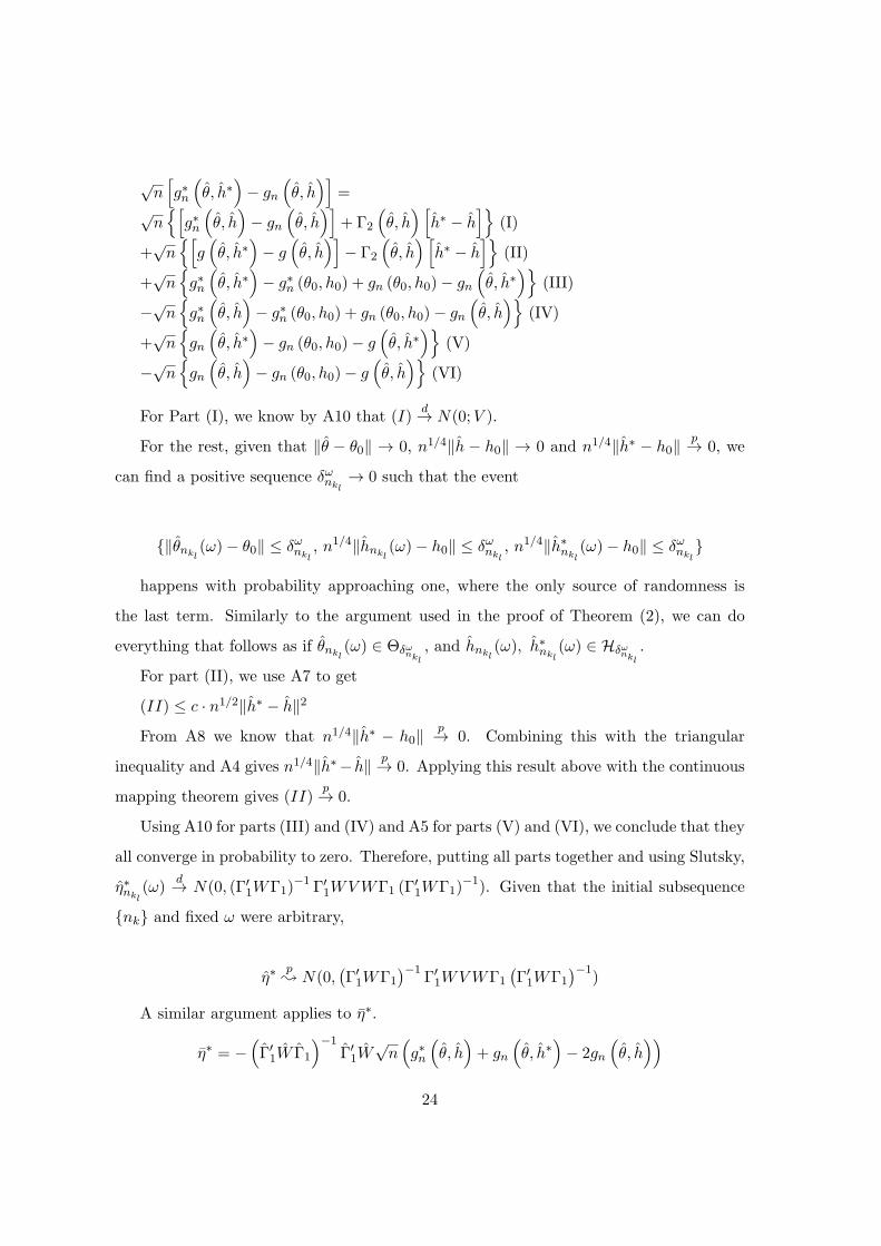
√n[

g∗n(

θ, h∗)

− gn

(

θ, h)]

=√n[

g∗n(

θ, h)

− gn

(

θ, h)]

+ Γ2

(

θ, h) [

h∗ − h]

(I)

+√n[

g(

θ, h∗)

− g(

θ, h)]

− Γ2

(

θ, h) [

h∗ − h]

(II)

+√n

g∗n(

θ, h∗)

− g∗n (θ0, h0) + gn (θ0, h0)− gn

(

θ, h∗)

(III)

−√n

g∗n(

θ, h)

− g∗n (θ0, h0) + gn (θ0, h0)− gn

(

θ, h)

(IV)

+√n

gn

(

θ, h∗)

− gn (θ0, h0)− g(

θ, h∗)

(V)

−√n

gn

(

θ, h)

− gn (θ0, h0)− g(

θ, h)

(VI)

For Part (I), we know by A10 that (I)d→ N(0;V ).

For the rest, given that ‖θ − θ0‖ → 0, n1/4‖h − h0‖ → 0 and n1/4‖h∗ − h0‖p→ 0, we

can find a positive sequence δωnkl→ 0 such that the event

‖θnkl(ω)− θ0‖ ≤ δωnkl

, n1/4‖hnkl(ω)− h0‖ ≤ δωnkl

, n1/4‖h∗nkl(ω)− h0‖ ≤ δωnkl

happens with probability approaching one, where the only source of randomness is

the last term. Similarly to the argument used in the proof of Theorem (2), we can do

everything that follows as if θnkl(ω) ∈ Θδωnkl

, and hnkl(ω), h∗nkl

(ω) ∈ Hδωnkl

.

For part (II), we use A7 to get

(II) ≤ c · n1/2‖h∗ − h‖2

From A8 we know that n1/4‖h∗ − h0‖p→ 0. Combining this with the triangular

inequality and A4 gives n1/4‖h∗− h‖ p→ 0. Applying this result above with the continuous

mapping theorem gives (II)p→ 0.

Using A10 for parts (III) and (IV) and A5 for parts (V) and (VI), we conclude that they

all converge in probability to zero. Therefore, putting all parts together and using Slutsky,

η∗nkl(ω)

d→ N(0, (Γ′1WΓ1)

−1 Γ′1WVWΓ1 (Γ

′1WΓ1)

−1). Given that the initial subsequence

nk and fixed ω were arbitrary,

η∗p; N(0,

(

Γ′1WΓ1

)−1Γ′1WVWΓ1

(

Γ′1WΓ1

)−1)

A similar argument applies to η∗.

η∗ = −(

Γ′1W Γ1

)−1Γ′1W

√n(

g∗n(

θ, h)

+ gn

(

θ, h∗)

− 2gn

(

θ, h))

24

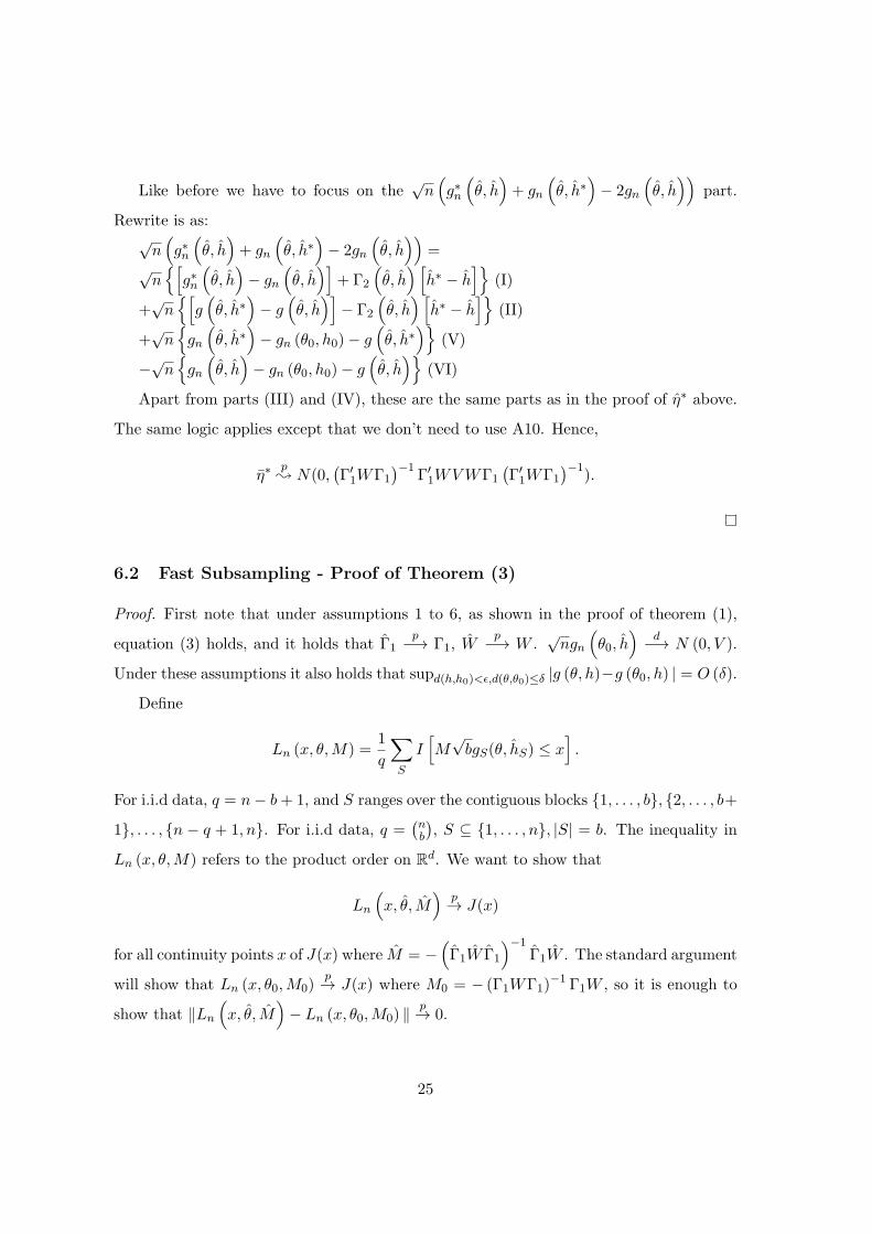
Like before we have to focus on the√n(

g∗n(

θ, h)

+ gn

(

θ, h∗)

− 2gn

(

θ, h))

part.

Rewrite is as:√n(

g∗n(

θ, h)

+ gn

(

θ, h∗)

− 2gn

(

θ, h))

=√n[

g∗n(

θ, h)

− gn

(

θ, h)]

+ Γ2

(

θ, h) [

h∗ − h]

(I)

+√n[

g(

θ, h∗)

− g(

θ, h)]

− Γ2

(

θ, h) [

h∗ − h]

(II)

+√n

gn

(

θ, h∗)

− gn (θ0, h0)− g(

θ, h∗)

(V)

−√n

gn

(

θ, h)

− gn (θ0, h0)− g(

θ, h)

(VI)

Apart from parts (III) and (IV), these are the same parts as in the proof of η∗ above.

The same logic applies except that we don’t need to use A10. Hence,

η∗p; N(0,

(

Γ′1WΓ1

)−1Γ′1WVWΓ1

(

Γ′1WΓ1

)−1).

6.2 Fast Subsampling - Proof of Theorem (3)

Proof. First note that under assumptions 1 to 6, as shown in the proof of theorem (1),

equation (3) holds, and it holds that Γ1p−→ Γ1, W

p−→ W .√ngn

(

θ0, h)

d−→ N (0, V ).

Under these assumptions it also holds that supd(h,h0)<ǫ,d(θ,θ0)≤δ |g (θ, h)−g (θ0, h) | = O (δ).

Define

Ln (x, θ,M) =1

q

∑

S

I[

M√bgS(θ, hS) ≤ x

]

.

For i.i.d data, q = n− b+ 1, and S ranges over the contiguous blocks 1, . . . , b, 2, . . . , b+1, . . . , n − q + 1, n. For i.i.d data, q =

(

nb

)

, S ⊆ 1, . . . , n, |S| = b. The inequality in

Ln (x, θ,M) refers to the product order on Rd. We want to show that

Ln

(

x, θ, M)

p→ J(x)

for all continuity points x of J(x) where M = −(

Γ1W Γ1

)−1Γ1W . The standard argument

will show that Ln (x, θ0,M0)p→ J(x) where M0 = − (Γ1WΓ1)

−1 Γ1W , so it is enough to

show that ‖Ln

(

x, θ, M)

− Ln (x, θ0,M0) ‖p→ 0.

25

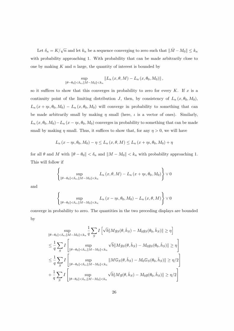
Let δn = K/√n and let kn be a sequence converging to zero such that ‖M −M0‖ ≤ kn

with probability approaching 1. With probability that can be made arbitrarily close to

one by making K and n large, the quantity of interest is bounded by

sup‖θ−θ0‖<δn,‖M−M0‖<kn

‖Ln (x, θ,M)− Ln (x, θ0,M0)‖ ,

so it suffices to show that this converges in probability to zero for every K. If x is a

continuity point of the limiting distribution J , then, by consistency of Ln (x, θ0,M0),

Ln (x+ ηι, θ0,M0) − Ln (x, θ0,M0) will converge in probability to something that can

be made arbitrarily small by making η small (here, ι is a vector of ones). Similarly,

Ln (x, θ0,M0)−Ln (x− ηι, θ0,M0) converges in probability to something that can be made

small by making η small. Thus, it suffices to show that, for any η > 0, we will have

Ln (x− ηι, θ0,M0)− η ≤ Ln (x, θ,M) ≤ Ln (x+ ηι, θ0,M0) + η

for all θ and M with ‖θ − θ0‖ < δn and ‖M −M0‖ < kn with probability approaching 1.

This will follow if

sup‖θ−θ0‖<δn,‖M−M0‖<kn

Ln (x, θ,M)− Ln (x+ ηι, θ0,M0)

∨ 0

and

sup‖θ−θ0‖<δn,‖M−M0‖<kn

Ln (x− ηι, θ0,M0)− Ln (x, θ,M)

∨ 0

converge in probability to zero. The quantities in the two preceding displays are bounded

by

sup‖θ−θ0‖<δn,‖M−M0‖<kn

1

q

∑

S

I[√

b‖MgS(θ, hS)−M0gS(θ0, hS)‖ ≥ η]

≤ 1

q

∑

S

I

[

sup‖θ−θ0‖<δn,‖M−M0‖<kn

√b‖MgS(θ, hS)−M0gS(θ0, hS)‖ ≥ η

]

≤ 1

q

∑

S

I

[

sup‖θ−θ0‖<δn,‖M−M0‖<kn

‖MGS(θ, hS)−M0GS(θ0, hS)‖ ≥ η/2

]

+1

q

∑

S

I

[

sup‖θ−θ0‖<δn,‖M−M0‖<kn

√b‖Mg(θ, hS)−M0g(θ0, hS)‖ ≥ η/2

]

26

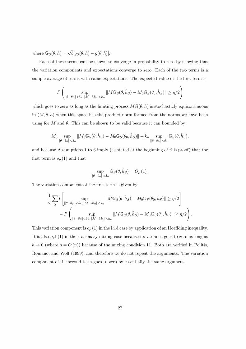
where GS(θ, h) =√b[gS(θ, h)− g(θ, h)].

Each of these terms can be shown to converge in probability to zero by showing that

the variation components and expectations converge to zero. Each of the two terms is a

sample average of terms with same expectations. The expected value of the first term is

P

(

sup‖θ−θ0‖<δn,‖M−M0‖<kn

‖MGS(θ, hS)−M0GS(θ0, hS)‖ ≥ η/2

)

which goes to zero as long as the limiting process MG(θ, h) is stochasticly equicontinuous

in (M, θ, h) when this space has the product norm formed from the norms we have been

using for M and θ. This can be shown to be valid because it can bounded by

M0 sup‖θ−θ0‖<δn

‖M0GS(θ, hS)−M0GS(θ0, hS)‖+ kn sup‖θ−θ0‖<δn

GS(θ, hS),

and because Assumptions 1 to 6 imply (as stated at the beginning of this proof) that the

first term is op (1) and that

sup‖θ−θ0‖<δn

GS(θ, hS) = Op (1) .

The variation component of the first term is given by

1

q

∑

S

I

[

sup‖θ−θ0‖<δn,‖M−M0‖<kn

‖MGS(θ, hS)−M0GS(θ0, hS)‖ ≥ η/2

]

− P

(

sup‖θ−θ0‖<δn,‖M−M0‖<kn

‖MGS(θ, hS)−M0GS(θ0, hS)‖ ≥ η/2

)

.

This variation component is op (1) in the i.i.d case by application of an Hoeffding inequality.

It is also op1 (1) in the stationary mixing case because its variance goes to zero as long as

b → 0 (where q = O (n)) because of the mixing condition 11. Both are verified in Politis,

Romano, and Wolf (1999), and therefore we do not repeat the arguments. The variation

component of the second term goes to zero by essentially the same argument.

27

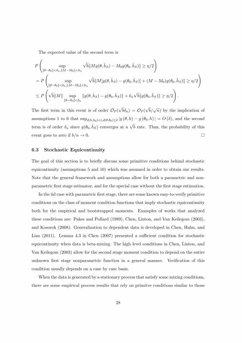
The expected value of the second term is

P

(

sup‖θ−θ0‖<δn,‖M−M0‖<kn

√b‖Mg(θ, hS)−M0g(θ0, hS)‖ ≥ η/2

)

= P

(

sup‖θ−θ0‖<δn,‖M−M0‖<kn

√b‖M [g(θ, hS)− g(θ0, hS)] + (M −M0)g(θ0, hS)‖ ≥ η/2

)

≤ P

(

√b‖M‖ sup

‖θ−θ0‖<δn

‖g(θ, hS)− g(θ0, hS)‖+ kn√b‖g(θ0, hS)‖ ≥ η/2

)

.

The first term in this event is of order OP (√bδn) = OP (

√b/√n) by the implication of

assumptions 1 to 6 that supd(h,h0)<ǫ,d(θ,θ0)≤δ |g (θ, h) − g (θ0, h) | = O (δ), and the second

term is of order δn since g(θ0, hS) converges at a√b rate. Thus, the probability of this

event goes to zero if b/n→ 0.

6.3 Stochastic Equicontinuity

The goal of this section is to briefly discuss some primitive conditions behind stochastic

equicontinuity (assumptions 5 and 10) which was assumed in order to obtain our results.

Note that the general framework and assumptions allow for both a parametric and non-

parametric first stage estimator, and for the special case without the first stage estimation.

In the iid case with parametric first stage, there are some known easy-to-verify primitive

conditions on the class of moment condition functions that imply stochastic equicontinuity

both for the empirical and bootstrapped moments. Examples of works that analyzed

these conditions are: Pakes and Pollard (1989), Chen, Linton, and Van Keilegom (2003),

and Kosorok (2008). Generalization to dependent data is developed in Chen, Hahn, and

Liao (2011). Lemma 4.3 in Chen (2007) presented a sufficient condition for stochastic

equicontinuity when data is beta-mixing. The high level conditions in Chen, Linton, and

Van Keilegom (2003) allow for the second stage moment condition to depend on the entire

unknown first stage nonparametric function in a general manner. Verification of this

condition usually depends on a case by case basis.

When the data is generated by a stationary process that satisfy some mixing conditions,

there are some empirical process results that rely on primitve conditions similar to those

28

mentioned above, and that are easier to verify when the first stage is parametric. We’ll

state these conditions and results below.

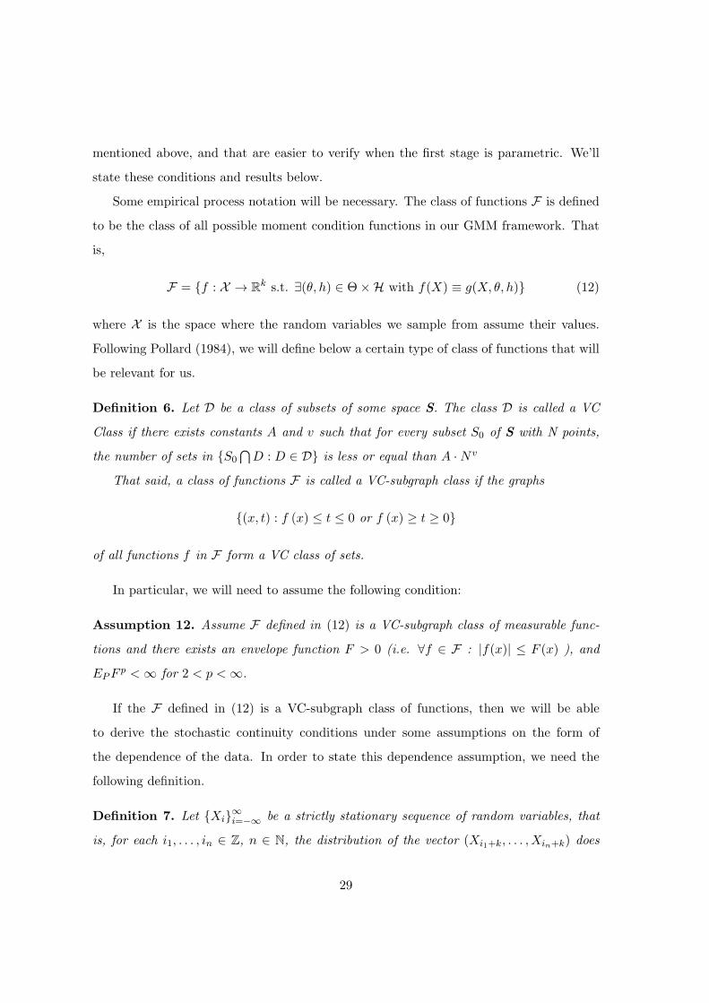
Some empirical process notation will be necessary. The class of functions F is defined

to be the class of all possible moment condition functions in our GMM framework. That

is,

F = f : X → Rk s.t. ∃(θ, h) ∈ Θ×H with f(X) ≡ g(X, θ, h) (12)

where X is the space where the random variables we sample from assume their values.

Following Pollard (1984), we will define below a certain type of class of functions that will

be relevant for us.

Definition 6. Let D be a class of subsets of some space S. The class D is called a VC

Class if there exists constants A and v such that for every subset S0 of S with N points,

the number of sets in S0⋂

D : D ∈ D is less or equal than A ·Nv

That said, a class of functions F is called a VC-subgraph class if the graphs

(x, t) : f (x) ≤ t ≤ 0 or f (x) ≥ t ≥ 0

of all functions f in F form a VC class of sets.

In particular, we will need to assume the following condition:

Assumption 12. Assume F defined in (12) is a VC-subgraph class of measurable func-

tions and there exists an envelope function F > 0 (i.e. ∀f ∈ F : |f(x)| ≤ F (x) ), and

EPFp <∞ for 2 < p <∞.

If the F defined in (12) is a VC-subgraph class of functions, then we will be able

to derive the stochastic continuity conditions under some assumptions on the form of

the dependence of the data. In order to state this dependence assumption, we need the

following definition.

Definition 7. Let Xi∞i=−∞ be a strictly stationary sequence of random variables, that

is, for each i1, . . . , in ∈ Z, n ∈ N, the distribution of the vector (Xi1+k, . . . , Xin+k) does

29

not depend on k ∈ Z. Define the following sigma-algebras A0 = σ (Xi : i ≤ 0) and Bn =

σ (Xi : i ≥ n). The β-mixing coefficient of dependence is given:

βn = β (A0,Bn) =1

2sup

∑

(i,j)∈I×J

|P (Ai ∩Bj)− P (Ai)P (Bj)|

where the sup is taken over all finite measurable partitions Aii∈I and Bii∈J of A0 and

Bn, respectively.

Before we move on to the actual assumptions and results, we need to define the

following real-valued mappings on F . P (f) = EP (f), where the expectation is taken

with respect to the distribution P of the data; Pn (f) = 1n

∑ni=1 f (Xi); and vn (f) =

n1/2 (Pn − P ) (f). In terms of the GMM framework, if f(X) ≡ g(X, θ, h), then P (f) =

g(θ, h), Pn(f) = gn(θ, h), and vn(f) = n1/2(gn(θ, h)− g(θ, h))

Lemma 4.2 in Chen (2007) provides a set of sufficient conditions for stochastic equicon-

tinuity when the data is beta-mixing. We briefly summarize her conditions and refer the

reader to details of the original Handbook of Econometrics Chapter in Chen (2007).

Proposition 1. (Lemma 4.2, Chen (2007)) If (1) Xi∞i=−∞ is a strictly stationary se-

quence of random variables with∑∞

k=1 k2

r−2βk < ∞ for some r > 2; (2) The moment

conditions and the first step function only depend on finitely many Xi; (3) Each of the

moment conditions is a sum of a Holder continuous component and a component that is

locally uniformly Lr(P ) continuous with respect to both the second stage parameter and the

first stage nonparametric function; (4) The parameter space of the second stage parameter

is compact, and the parameter space of the first stage nonparametric function has a finite

covering entropy, then

supf∈Fδn

|vn (f)− vn (f0)|p→ 0

where f0(X) = g(X, θ0, h0), and Fδn stands for an open δn-ball in F around f0.

The finite covering entropy part of condition (4) can be derived from assumption (12).

If we are willing to strengthen the assumption on the β-mixing type of dependence, we

can also obtain stochastic equicontinuity on the bootstrapped moments, a result derived

30

in Radulovic (1996). Similarly to before, define the real-valued bootstrap counterparts of

the mappings on F : P ∗n (f) = 1

n

∑ni=1 f (X

∗i ); and v

∗n (f) = n1/2 (P ∗

n − Pn) (f). Here, we

shall use the MBB procedure to generate X∗, according to definition 2.

Assumption 13. Assume Xi∞i=−∞ is a strictly stationary sequence of random variables

such that kp

p−2 (log k)2 p−1

p−2 βk →k→∞

0 for the p in assumption(12). Further assume that for

some q > p/ (p− 2) such that kq > kp

p−2 (log k)2 p−1

p−2 for big k, the β-mixing coefficient of

the stationary sequence also satisfies kqβk = O (1). Also assume that in MBB procedure,

the number of blocks b (n) →n→∞

∞ and b (n) = O (nρ) for some 0 < ρ < p−22(p−1) .

The following proposition is due to Radulovic (1996).

Proposition 2. Suppose assumptions 12 to 13 hold, and that the bootstrap sample is

generated according to the MBB procedure. Then, for any positive sequence δn = o(1), we

have both:

supf∈Fδn

|vn (f)− vn (f0)|p→ 0

and

supf∈Fδn

|v∗n (f)− v∗n (f0)|p; 0.

31

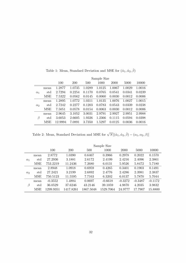
Table 1: Mean, Standard Deviation and MSE for (α1, α2, β)

Sample Size100 200 500 1000 2000 5000 10000

mean 1.2877 1.0735 1.0289 1.0125 1.0067 1.0029 1.0016α1 std 2.7294 0.2254 0.1170 0.0765 0.0541 0.0341 0.0239

MSE 7.5322 0.0562 0.0145 0.0060 0.0030 0.0012 0.0006

mean 1.2895 1.0772 1.0311 1.0135 1.0076 1.0027 1.0015α2 std 2.7242 0.2277 0.1203 0.0783 0.0543 0.0339 0.0238

MSE 7.5051 0.0578 0.0154 0.0063 0.0030 0.0012 0.0006

mean 2.9645 3.1052 3.0031 2.9791 2.9927 2.9951 2.9988β std 3.6053 2.6605 1.9326 1.2366 0.1115 0.0594 0.0398

MSE 12.9994 7.0891 3.7350 1.5297 0.0125 0.0036 0.0016

Table 2: Mean, Standard Deviation and MSE for√N [(α1, α2, β)− (α1, α2, β)]

Sample Size100 200 500 1000 2000 5000 10000

mean 2.8772 1.0390 0.6467 0.3966 0.2978 0.2022 0.1570α1 std 27.2936 3.1881 2.6172 2.4199 2.4216 2.4096 2.3861

MSE 753.2219 11.2436 7.2680 6.0131 5.9526 5.8472 5.7180

mean 2.8948 1.0918 0.6959 0.4265 0.3401 0.1903 0.1491α2 std 27.2421 3.2199 2.6892 2.4776 2.4286 2.3981 2.3837

MSE 750.5123 11.5595 7.7163 6.3202 6.0137 5.7870 5.7044

mean -0.3552 1.4884 0.0697 -0.6618 -0.3272 -0.3487 -0.1172β std 36.0529 37.6246 43.2146 39.1059 4.9870 4.2035 3.9832

MSE 1299.9351 1417.8261 1867.5048 1529.7064 24.9777 17.7907 15.8800

32

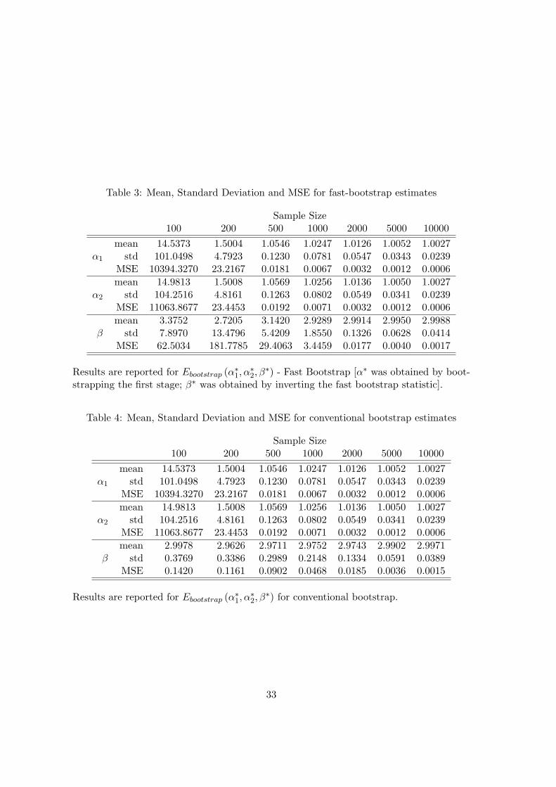
Table 3: Mean, Standard Deviation and MSE for fast-bootstrap estimates

Sample Size100 200 500 1000 2000 5000 10000

mean 14.5373 1.5004 1.0546 1.0247 1.0126 1.0052 1.0027α1 std 101.0498 4.7923 0.1230 0.0781 0.0547 0.0343 0.0239

MSE 10394.3270 23.2167 0.0181 0.0067 0.0032 0.0012 0.0006

mean 14.9813 1.5008 1.0569 1.0256 1.0136 1.0050 1.0027α2 std 104.2516 4.8161 0.1263 0.0802 0.0549 0.0341 0.0239

MSE 11063.8677 23.4453 0.0192 0.0071 0.0032 0.0012 0.0006

mean 3.3752 2.7205 3.1420 2.9289 2.9914 2.9950 2.9988β std 7.8970 13.4796 5.4209 1.8550 0.1326 0.0628 0.0414

MSE 62.5034 181.7785 29.4063 3.4459 0.0177 0.0040 0.0017

Results are reported for Ebootstrap (α∗1, α

∗2, β

∗) - Fast Bootstrap [α∗ was obtained by boot-strapping the first stage; β∗ was obtained by inverting the fast bootstrap statistic].

Table 4: Mean, Standard Deviation and MSE for conventional bootstrap estimates

Sample Size100 200 500 1000 2000 5000 10000

mean 14.5373 1.5004 1.0546 1.0247 1.0126 1.0052 1.0027α1 std 101.0498 4.7923 0.1230 0.0781 0.0547 0.0343 0.0239

MSE 10394.3270 23.2167 0.0181 0.0067 0.0032 0.0012 0.0006

mean 14.9813 1.5008 1.0569 1.0256 1.0136 1.0050 1.0027α2 std 104.2516 4.8161 0.1263 0.0802 0.0549 0.0341 0.0239

MSE 11063.8677 23.4453 0.0192 0.0071 0.0032 0.0012 0.0006

mean 2.9978 2.9626 2.9711 2.9752 2.9743 2.9902 2.9971β std 0.3769 0.3386 0.2989 0.2148 0.1334 0.0591 0.0389

MSE 0.1420 0.1161 0.0902 0.0468 0.0185 0.0036 0.0015

Results are reported for Ebootstrap (α∗1, α

∗2, β

∗) for conventional bootstrap.

33

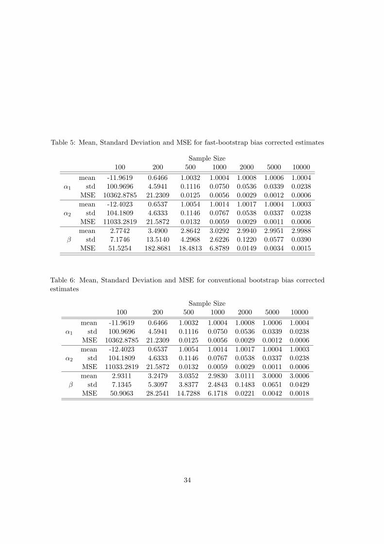
Table 5: Mean, Standard Deviation and MSE for fast-bootstrap bias corrected estimates

Sample Size100 200 500 1000 2000 5000 10000

mean -11.9619 0.6466 1.0032 1.0004 1.0008 1.0006 1.0004α1 std 100.9696 4.5941 0.1116 0.0750 0.0536 0.0339 0.0238

MSE 10362.8785 21.2309 0.0125 0.0056 0.0029 0.0012 0.0006

mean -12.4023 0.6537 1.0054 1.0014 1.0017 1.0004 1.0003α2 std 104.1809 4.6333 0.1146 0.0767 0.0538 0.0337 0.0238

MSE 11033.2819 21.5872 0.0132 0.0059 0.0029 0.0011 0.0006

mean 2.7742 3.4900 2.8642 3.0292 2.9940 2.9951 2.9988β std 7.1746 13.5140 4.2968 2.6226 0.1220 0.0577 0.0390

MSE 51.5254 182.8681 18.4813 6.8789 0.0149 0.0034 0.0015

Table 6: Mean, Standard Deviation and MSE for conventional bootstrap bias correctedestimates

Sample Size100 200 500 1000 2000 5000 10000

mean -11.9619 0.6466 1.0032 1.0004 1.0008 1.0006 1.0004α1 std 100.9696 4.5941 0.1116 0.0750 0.0536 0.0339 0.0238

MSE 10362.8785 21.2309 0.0125 0.0056 0.0029 0.0012 0.0006

mean -12.4023 0.6537 1.0054 1.0014 1.0017 1.0004 1.0003α2 std 104.1809 4.6333 0.1146 0.0767 0.0538 0.0337 0.0238

MSE 11033.2819 21.5872 0.0132 0.0059 0.0029 0.0011 0.0006

mean 2.9311 3.2479 3.0352 2.9830 3.0111 3.0000 3.0006β std 7.1345 5.3097 3.8377 2.4843 0.1483 0.0651 0.0429

MSE 50.9063 28.2541 14.7288 6.1718 0.0221 0.0042 0.0018

34

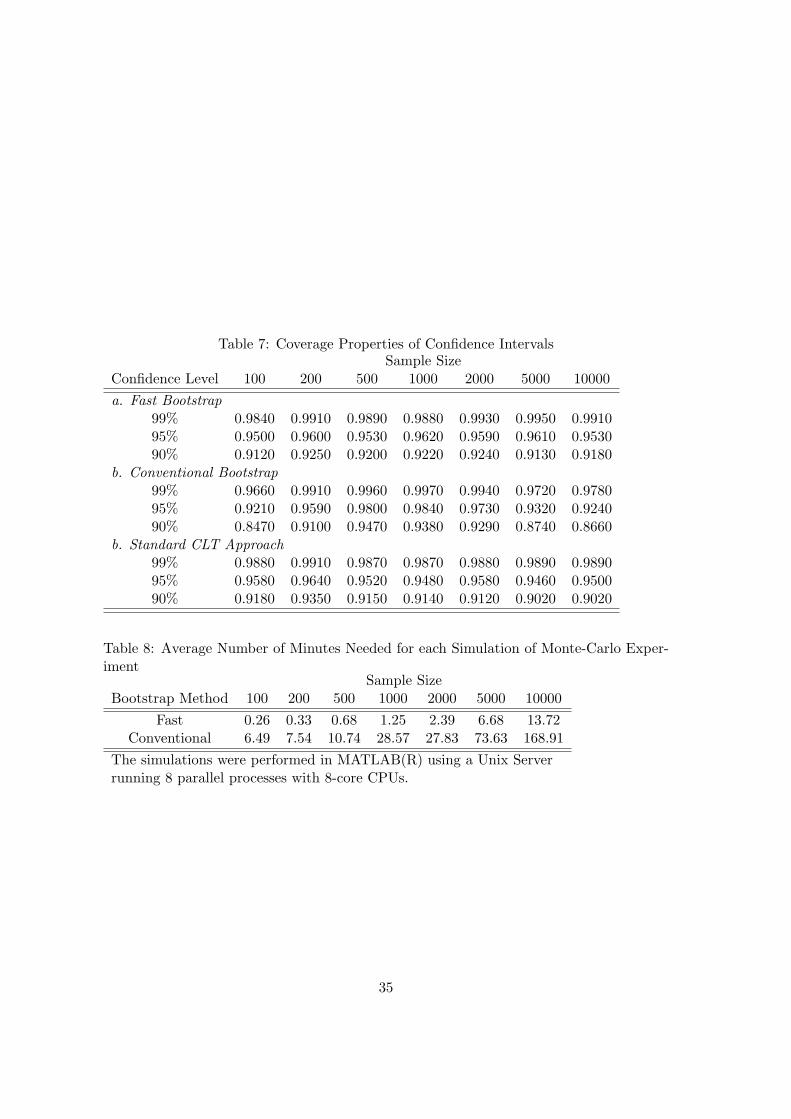
Table 7: Coverage Properties of Confidence IntervalsSample Size

Confidence Level 100 200 500 1000 2000 5000 10000

a. Fast Bootstrap99% 0.9840 0.9910 0.9890 0.9880 0.9930 0.9950 0.991095% 0.9500 0.9600 0.9530 0.9620 0.9590 0.9610 0.953090% 0.9120 0.9250 0.9200 0.9220 0.9240 0.9130 0.9180

b. Conventional Bootstrap99% 0.9660 0.9910 0.9960 0.9970 0.9940 0.9720 0.978095% 0.9210 0.9590 0.9800 0.9840 0.9730 0.9320 0.924090% 0.8470 0.9100 0.9470 0.9380 0.9290 0.8740 0.8660

b. Standard CLT Approach99% 0.9880 0.9910 0.9870 0.9870 0.9880 0.9890 0.989095% 0.9580 0.9640 0.9520 0.9480 0.9580 0.9460 0.950090% 0.9180 0.9350 0.9150 0.9140 0.9120 0.9020 0.9020

Table 8: Average Number of Minutes Needed for each Simulation of Monte-Carlo Exper-iment

Sample SizeBootstrap Method 100 200 500 1000 2000 5000 10000

Fast 0.26 0.33 0.68 1.25 2.39 6.68 13.72Conventional 6.49 7.54 10.74 28.57 27.83 73.63 168.91

The simulations were performed in MATLAB(R) using a Unix Serverrunning 8 parallel processes with 8-core CPUs.

35