A fast learning algorithm for deep belief nets ∗

Geoffrey E. Hinton and Simon OsinderoDepartment of Computer Science University of Toronto

10 Kings College Road

Toronto, Canada M5S 3G4

hinton, osindero@cs.toronto.edu

Yee-Whye TehDepartment of Computer Science

National University of Singapore

3 Science Drive 3, Singapore, 117543

tehyw@comp.nus.edu.sg

Abstract

We show how to use “complementary priors” toeliminate the explaining away effects that makeinference difficult in densely-connected beliefnets that have many hidden layers. Using com-plementary priors, we derive a fast, greedy algo-rithm that can learn deep, directed belief networksone layer at a time, provided the top two lay-ers form an undirected associative memory. Thefast, greedy algorithm is used to initialize a slowerlearning procedure that fine-tunes the weights us-ing a contrastive version of the wake-sleep algo-rithm. After fine-tuning, a network with threehidden layers forms a very good generative modelof the joint distribution of handwritten digit im-ages and their labels. This generative model givesbetter digit classification than the best discrimi-native learning algorithms. The low-dimensionalmanifolds on which the digits lie are modelled bylong ravines in the free-energy landscape of thetop-level associative memory and it is easy to ex-plore these ravines by using the directed connec-tions to display what the associative memory hasin mind.

1 Introduction

Learning is difficult in densely-connected, directed belief netsthat have many hidden layers because it is difficult to infer theconditional distribution of the hidden activities when given adata vector. Variational methods use simple approximationsto the true conditional distribution, but the approximationsmay be poor, especially at the deepest hidden layer wherethe prior assumes independence. Also, variational learningstill requires all of the parameters to be learned together andmakes the learning time scale poorly as the number of param-eters increases.

We describe a model in which the top two hidden layersform an undirected associative memory (see figure 1) and the

∗To appear in Neural Computation 2006

remaining hidden layers form a directed acyclic graph thatconverts the representations in the associative memory intoobservable variables such as the pixels of an image. This hy-brid model has some attractive features:

1. There is a fast, greedy learning algorithm that can finda fairly good set of parameters quickly, even in deepnetworks with millions of parameters and many hiddenlayers.

2. The learning algorithm is unsupervised but can be ap-plied to labeled data by learning a model that generatesboth the label and the data.

3. There is a fine-tuning algorithm that learns an excel-lent generative model which outperforms discrimina-tive methods on the MNIST database of hand-writtendigits.

4. The generative model makes it easy to interpret the dis-tributed representations in the deep hidden layers.

5. The inference required for forming a percept is both fastand accurate.

6. The learning algorithm is local: adjustments to asynapse strength depend only on the states of the pre-synaptic and post-synaptic neuron.

7. The communication is simple: neurons only need tocommunicate their stochastic binary states.

Section 2 introduces the idea of a “complementary” priorwhich exactly cancels the “explaining away” phenomenonthat makes inference difficult in directed models. An exam-ple of a directed belief network with complementary priorsis presented. Section 3 shows the equivalence between re-stricted Boltzmann machines and infinite directed networkswith tied weights.

Section 4 introduces a fast, greedy learning algorithmfor constructing multi-layer directed networks one layer ata time. Using a variational bound it shows that as each newlayer is added, the overall generative model improves. Thegreedy algorithm bears some resemblance to boosting in itsrepeated use of the same “weak” learner, but instead of re-weighting each data-vector to ensure that the next step learnssomething new, it re-represents it. The “weak” learner that

2000 top-level units

500 units

500 units

28 x 28

pixel

image

10 label units

This could be the

top level of

another sensory

pathway

Figure 1: The network used to model the joint distributionof digit images and digit labels. In this paper, each trainingcase consists of an image and an explicit class label, but workin progress has shown that the same learning algorithm canbe used if the “labels” are replaced by a multilayer pathwaywhose inputs are spectrograms from multiple different speak-ers saying isolated digits. The network then learns to generatepairs that consist of an image and a spectrogram of the samedigit class.

is used to construct deep directed nets is itself an undirectedgraphical model.

Section 5 shows how the weights produced by the fastgreedy algorithm can be fine-tuned using the “up-down” al-gorithm. This is a contrastive version of the wake-sleep al-gorithm Hinton et al. (1995) that does not suffer from the“mode-averaging” problems that can cause the wake-sleep al-gorithm to learn poor recognition weights.

Section 6 shows the pattern recognition performance ofa network with three hidden layers and about 1.7 millionweights on the MNIST set of handwritten digits. When noknowledge of geometry is provided and there is no specialpreprocessing, the generalization performance of the networkis 1.25% errors on the 10, 000 digit official test set. This beatsthe 1.5% achieved by the best back-propagation nets whenthey are not hand-crafted for this particular application. It isalso slightly better than the 1.4% errors reported by Decosteand Schoelkopf (2002) for support vector machines on thesame task.

Finally, section 7 shows what happens in the mind of thenetwork when it is running without being constrained by vi-sual input. The network has a full generative model, so it iseasy to look into its mind – we simply generate an image fromits high-level representations.

Throughout the paper, we will consider nets composed of

Figure 2: A simple logistic belief net containing two inde-pendent, rare causes that become highly anti-correlated whenwe observe the house jumping. The bias of −10 on the earth-quake node means that, in the absence of any observation, thisnode is e10 times more likely to be off than on. If the earth-quake node is on and the truck node is off, the jump node hasa total input of 0 which means that it has an even chance ofbeing on. This is a much better explanation of the observationthat the house jumped than the odds of e−20 which apply ifneither of the hidden causes is active. But it is wasteful to turnon both hidden causes to explain the observation because theprobability of them both happening is e−10 × e−10 = e−20.When the earthquake node is turned on it “explains away” theevidence for the truck node.

stochastic binary variables but the ideas can be generalized toother models in which the log probability of a variable is anadditive function of the states of its directly-connected neigh-bours (see Appendix A for details).

2 Complementary priors

The phenomenon of explaining away (illustrated in figure 2)makes inference difficult in directed belief nets. In denselyconnected networks, the posterior distribution over the hid-den variables is intractable except in a few special cases suchas mixture models or linear models with additive Gaussiannoise. Markov Chain Monte Carlo methods (Neal, 1992) canbe used to sample from the posterior, but they are typicallyvery time consuming. Variational methods (Neal and Hinton,1998) approximate the true posterior with a more tractabledistribution and they can be used to improve a lower bound onthe log probability of the training data. It is comforting thatlearning is guaranteed to improve a variational bound evenwhen the inference of the hidden states is done incorrectly,but it would be much better to find a way of eliminating ex-plaining away altogether, even in models whose hidden vari-ables have highly correlated effects on the visible variables.It is widely assumed that this is impossible.

A logistic belief net (Neal, 1992) is composed of stochas-tic binary units. When the net is used to generate data, the

probability of turning on unit i is a logistic function of thestates of its immediate ancestors, j, and of the weights, wij ,on the directed connections from the ancestors:

p(si = 1) =1

1 + exp(−bi −∑

j sjwij)(1)

where bi is the bias of unit i. If a logistic belief net onlyhas one hidden layer, the prior distribution over the hiddenvariables is factorial because their binary states are chosenindependently when the model is used to generate data. Thenon-independence in the posterior distribution is created bythe likelihood term coming from the data. Perhaps we couldeliminate explaining away in the first hidden layer by usingextra hidden layers to create a “complementary” prior thathas exactly the opposite correlations to those in the likeli-hood term. Then, when the likelihood term is multiplied bythe prior, we will get a posterior that is exactly factorial. It isnot at all obvious that complementary priors exist, but figure 3shows a simple example of an infinite logistic belief net withtied weights in which the priors are complementary at everyhidden layer (see Appendix A for a more general treatment ofthe conditions under which complementary priors exist). Theuse of tied weights to construct complementary priors mayseem like a mere trick for making directed models equiva-lent to undirected ones. As we shall see, however, it leadsto a novel and very efficient learning algorithm that worksby progressively untying the weights in each layer from theweights in higher layers.

2.1 An infinite directed model with tied weights

We can generate data from the infinite directed net in fig-ure 3 by starting with a random configuration at an infinitelydeep hidden layer1 and then performing a top-down “ances-tral” pass in which the binary state of each variable in a layeris chosen from the Bernoulli distribution determined by thetop-down input coming from its active parents in the layerabove. In this respect, it is just like any other directed acyclicbelief net. Unlike other directed nets, however, we can sam-ple from the true posterior distribution over all of the hiddenlayers by starting with a data vector on the visible units andthen using the transposed weight matrices to infer the fac-torial distributions over each hidden layer in turn. At eachhidden layer we sample from the factorial posterior beforecomputing the factorial posterior for the layer above2. Ap-pendix A shows that this procedure gives unbiased samplesbecause the complementary prior at each layer ensures thatthe posterior distribution really is factorial.

Since we can sample from the true posterior, we can com-pute the derivatives of the log probability of the data. Let

1The generation process converges to the stationary distributionof the Markov Chain, so we need to start at a layer that is deepcompared with the time it takes for the chain to reach equilibrium.

2This is exactly the same as the inference procedure used in thewake-sleep algorithm (Hinton et al., 1995) for the models describedin this paper no variational approximation is required because theinference procedure gives unbiased samples.

us start by computing the derivative for a generative weight,w00

ij , from a unit j in layer H0 to unit i in layer V0 (see figure3). In a logistic belief net, the maximum likelihood learningrule for a single data-vector, v0, is:

∂ log p(v0)∂w00

ij

=<h0j (v

0i − v0

i )> (2)

where < ·> denotes an average over the sampled states andv0

i is the probability that unit i would be turned on if the visi-ble vector was stochastically reconstructed from the sampledhidden states. Computing the posterior distribution over thesecond hidden layer, V1, from the sampled binary states in thefirst hidden layer, H0, is exactly the same process as recon-structing the data, so v1

i is a sample from a Bernoulli randomvariable with probability v0

i . The learning rule can thereforebe written as:

∂ log p(v0)∂w00

ij

=<h0j (v

0i − v1

i )> (3)

The dependence of v1i on h0

j is unproblematic in the deriva-tion of Eq. 3 from Eq. 2 because v0

i is an expectation that isconditional on h0

j . Since the weights are replicated, the fullderivative for a generative weight is obtained by summing thederivatives of the generative weights between all pairs of lay-ers:

∂ log p(v0)∂wij

= <h0j (v

0i − v1

i )>

+ <v1i (h0

j − h1j )>

+ <h1j (v

1i − v2

i )>+... (4)

All of the vertically aligned terms cancel leaving the Boltz-mann machine learning rule of Eq. 5.

3 Restricted Boltzmann machines andcontrastive divergence learning

It may not be immediately obvious that the infinite directednet in figure 3 is equivalent to a Restricted Boltzmann Ma-chine (RBM). An RBM has a single layer of hidden unitswhich are not connected to each other and have undirected,symmetrical connections to a layer of visible units. To gen-erate data from an RBM, we can start with a random statein one of the layers and then perform alternating Gibbs sam-pling: All of the units in one layer are updated in parallelgiven the current states of the units in the other layer and thisis repeated until the system is sampling from its equilibriumdistribution. Notice that this is exactly the same process asgenerating data from the infinite belief net with tied weights.To perform maximum likelihood learning in an RBM, we canuse the difference between two correlations. For each weight,wij , between a visible unit i and a hidden unit, j we measurethe correlation < v0

i h0j > when a datavector is clamped on

W

V1

H1

V0

H0

V2

TW

TW

W

W

etc.

0

iv

0

jh

1

jh

1

iv

2

iv

TW

TW

TW

W

W

Figure 3: An infinite logistic belief net with tied weights. Thedownward arrows represent the generative model. The up-ward arrows are not part of the model. They represent theparameters that are used to infer samples from the posteriordistribution at each hidden layer of the net when a datavectoris clamped on V0.

the visible units and the hidden states are sampled from theirconditional distribution, which is factorial. Then, using al-ternating Gibbs sampling, we run the Markov chain shown infigure 4 until it reaches its stationary distribution and measurethe correlation <v∞i h∞

j >. The gradient of the log probabilityof the training data is then

∂ log p(v0)∂wij

=<v0i h0

j> − <v∞i h∞

j > (5)

This learning rule is the same as the maximum likelihoodlearning rule for the infinite logistic belief net with tiedweights, and each step of Gibbs sampling corresponds tocomputing the exact posterior distribution in a layer of theinfinite logistic belief net.

Maximizing the log probability of the data is exactlythe same as minimizing the Kullback-Leibler divergence,KL(P 0||P∞

θ ), between the distribution of the data, P 0, andthe equilibrium distribution defined by the model, P∞

θ . Incontrastive divergence learning (Hinton, 2002), we only runthe Markov chain for n full steps3 before measuring the sec-ond correlation. This is equivalent to ignoring the derivatives

3Each full step consists of updating h given v then updating vgiven h.

>< 00

ji hv

i

j

i

j

i

j

i

j

t = 0 t = 1 t = 2 t = infinity

t = 0 t = 1 t = 2 t = infinity

>< ∞∞ji hv

Figure 4: This depicts a Markov chain that uses alternatingGibbs sampling. In one full step of Gibbs sampling, the hid-den units in the top layer are all updated in parallel by apply-ing Eq. 1 to the inputs received from the the current statesof the visible units in the bottom layer, then the visible unitsare all updated in parallel given the current hidden states. Thechain is initialized by setting the binary states of the visibleunits to be the same as a data-vector. The correlations in theactivities of a visible and a hidden unit are measured after thefirst update of the hidden units and again at the end of thechain. The difference of these two correlations provides thelearning signal for updating the weight on the connection.

that come from the higher layers of the infinite net. The sumof all these ignored derivatives is the derivative of the logprobability of the posterior distribution in layer Vn, whichis also the derivative of the Kullback-Leibler divergence be-tween the posterior distribution in layer Vn, Pn

θ , and the equi-librium distribution defined by the model. So contrastive di-vergence learning minimizes the difference of two Kullback-Leibler divergences:

KL(P 0||P∞θ ) − KL(Pn

θ ||P∞θ ) (6)

Ignoring sampling noise, this difference is never negativebecause Gibbs sampling is used to produce Pn

θ from P 0 andGibbs sampling always reduces the Kullback-Leibler diver-gence with the equilibrium distribution. It is important to no-tice that Pn

θ depends on the current model parameters andthe way in which Pn

θ changes as the parameters change isbeing ignored by contrastive divergence learning. This prob-lem does not arise with P 0 because the training data does notdepend on the parameters. An empirical investigation of therelationship between the maximum likelihood and the con-trastive divergence learning rules can be found in Carreira-Perpinan and Hinton (2005).

Contrastive divergence learning in a restricted Boltzmannmachine is efficient enough to be practical (Mayraz and Hin-ton, 2001). Variations that use real-valued units and differ-ent sampling schemes are described in Teh et al. (2003) andhave been quite successful for modeling the formation of to-pographic maps (Welling et al., 2003), for denoising naturalimages (Roth and Black, 2005) or images of biological cells(Ning et al., 2005). Marks and Movellan (2001) describe away of using contrastive divergence to perform factor analy-sis and Welling et al. (2005) show that a network with logistic,binary visible units and linear, Gaussian hidden units can beused for rapid document retrieval. However, it appears that

the efficiency has been bought at a high price: When appliedin the obvious way, contrastive divergence learning fails fordeep, multilayer networks with different weights at each layerbecause these networks take far too long even to reach condi-tional equilibrium with a clamped data-vector. We now showthat the equivalence between RBM’s and infinite directed netswith tied weights suggests an efficient learning algorithm formultilayer networks in which the weights are not tied.

4 A greedy learning algorithm fortransforming representations

An efficient way to learn a complicated model is to combinea set of simpler models that are learned sequentially. To forceeach model in the sequence to learn something different fromthe previous models, the data is modified in some way aftereach model has been learned. In boosting (Freund, 1995),each model in the sequence is trained on re-weighted data thatemphasizes the cases that the preceding models got wrong. Inone version of principal components analysis, the variance ina modeled direction is removed thus forcing the next modeleddirection to lie in the orthogonal subspace (Sanger, 1989).In projection pursuit (Friedman and Stuetzle, 1981), the datais transformed by nonlinearly distorting one direction in thedata-space to remove all non-Gaussianity in that direction.The idea behind our greedy algorithm is to allow each modelin the sequence to receive a different representation of thedata. The model performs a non-linear transformation on itsinput vectors and produces as output the vectors that will beused as input for the next model in the sequence.

Figure 5 shows a multilayer generative model in which thetop two layers interact via undirected connections and all ofthe other connections are directed. The undirected connec-tions at the top are equivalent to having infinitely many higherlayers with tied weights. There are no intra-layer connectionsand, to simplify the analysis, all layers have the same numberof units. It is possible to learn sensible (though not optimal)values for the parameters W0 by assuming that the parame-ters between higher layers will be used to construct a comple-mentary prior for W0. This is equivalent to assuming that allof the weight matrices are constrained to be equal. The taskof learning W0 under this assumption reduces to the task oflearning an RBM and although this is still difficult, good ap-proximate solutions can be found rapidly by minimizing con-trastive divergence. Once W0 has been learned, the data canbe mapped through WT

0 to create higher-level “data” at thefirst hidden layer.

If the RBM is a perfect model of the original data, thehigher-level “data” will already be modeled perfectly by thehigher-level weight matrices. Generally, however, the RBMwill not be able to model the original data perfectly and wecan make the generative model better using the followinggreedy algorithm:

1. Learn W0 assuming all the weight matrices are tied.

2. Freeze W0 and commit ourselves to using WT0 to infer

Figure 5: A hybrid network. The top two layers have undi-rected connections and form an associative memory. The lay-ers below have directed, top-down, generative connectionsthat can be used to map a state of the associative memoryto an image. There are also directed, bottom-up, recognitionconnections that are used to infer a factorial representation inone layer from the binary activities in the layer below. In thegreedy initial learning the recognition connections are tied tothe generative connections.

factorial approximate posterior distributions over thestates of the variables in the first hidden layer, even ifsubsequent changes in higher level weights mean thatthis inference method is no longer correct.

3. Keeping all the higher weight matrices tied to eachother, but untied from W0, learn an RBM model of thehigher-level “data” that was produced by using WT

0 totransform the original data.

If this greedy algorithm changes the higher-level weightmatrices, it is guaranteed to improve the generative model.As shown in (Neal and Hinton, 1998), the negative log prob-ability of a single data-vector, v0, under the multilayer gen-erative model is bounded by a variational free energy whichis the expected energy under the approximating distribution,Q(h0|v0), minus the entropy of that distribution. For a di-rected model, the “energy” of the configuration v0,h0 isgiven by:

E(v0,h0) = − [log p(h0) + log p(v0|h0)

](7)

So the bound is:

log p(v0) ≥∑

all h0

Q(h0|v0)[log p(h0) + log p(v0|h0)

]

−∑

all h0

Q(h0|v0) log Q(h0|v0) (8)

where h0 is a binary configuration of the units in the first hid-den layer, p(h0) is the prior probability of h0 under the cur-rent model (which is defined by the weights above H0) andQ(·|v0) is any probability distribution over the binary con-figurations in the first hidden layer. The bound becomes anequality if and only if Q(·|v0) is the true posterior distribu-tion.

When all of the weight matrices are tied together, the fac-torial distribution over H0 produced by applying WT

0 to adata-vector is the true posterior distribution, so at step 2 ofthe greedy algorithm log p(v0) is equal to the bound. Step2 freezes both Q(·|v0) and p(v0|h0) and with these termsfixed, the derivative of the bound is the same as the derivativeof ∑

all h0

Q(h0|v0) log p(h0) (9)

So maximizing the bound w.r.t. the weights in the higher lay-ers is exactly equivalent to maximizing the log probability ofa dataset in which h0 occurs with probability Q(h0|v0). Ifthe bound becomes tighter, it is possible for log p(v0) to falleven though the lower bound on it increases, but log p(v0)can never fall below its value at step 2 of the greedy algo-rithm because the bound is tight at this point and the boundalways increases.

The greedy algorithm can clearly be applied recursively,so if we use the full maximum likelihood Boltzmann machinelearning algorithm to learn each set of tied weights and thenwe untie the bottom layer of the set from the weights above,we can learn the weights one layer at a time with a guar-antee4 that we will never decrease the log probability of thedata under the full generative model. In practice, we replacemaximum likelihood Boltzmann machine learning algorithmby contrastive divergence learning because it works well andis much faster. The use of contrastive divergence voids theguarantee, but it is still reassuring to know that extra layersare guaranteed to improve imperfect models if we learn eachlayer with sufficient patience.

To guarantee that the generative model is improved bygreedily learning more layers, it is convenient to considermodels in which all layers are the same size so that the higher-level weights can be initialized to the values learned beforethey are untied from the weights in the layer below. The samegreedy algorithm, however, can be applied even when the lay-ers are different sizes.

5 Back-Fitting with the up-down algorithm

Learning the weight matrices one layer at a time is efficientbut not optimal. Once the weights in higher layers have beenlearned, neither the weights nor the simple inference proce-dure are optimal for the lower layers. The sub-optimality pro-duced by greedy learning is relatively innocuous for super-vised methods like boosting. Labels are often scarce and each

4The guarantee is on the expected change in the log probability.

label may only provide a few bits of constraint on the parame-ters, so over-fitting is typically more of a problem than under-fitting. Going back and refitting the earlier models may, there-fore, cause more harm than good. Unsupervised methods,however, can use very large unlabeled datasets and each casemay be very high-dimensional thus providing many bits ofconstraint on a generative model. Under-fitting is then a se-rious problem which can be alleviated by a subsequent stageof back-fitting in which the weights that were learned first arerevised to fit in better with the weights that were learned later.

After greedily learning good initial values for the weightsin every layer, we untie the “recognition” weights that areused for inference from the “generative” weights that de-fine the model, but retain the restriction that the posterior ineach layer must be approximated by a factorial distribution inwhich the variables within a layer are conditionally indepen-dent given the values of the variables in the layer below. Avariant of the wake-sleep algorithm described in Hinton et al.(1995) can then be used to allow the higher-level weights toinfluence the lower level ones. In the “up-pass”, the recog-nition weights are used in a bottom-up pass that stochasti-cally picks a state for every hidden variable. The generativeweights on the directed connections are then adjusted usingthe maximum likelihood learning rule in Eq. 25. The weightson the undirected connections at the top level are learned asbefore by fitting the top-level RBM to the posterior distribu-tion of the penultimate layer.

The “down-pass” starts with a state of the top-level asso-ciative memory and uses the top-down generative connectionsto stochastically activate each lower layer in turn. Duringthe down-pass, the top-level undirected connections and thegenerative directed connections are not changed. Only thebottom-up recognition weights are modified. This is equiva-lent to the sleep phase of the wake-sleep algorithm if the as-sociative memory is allowed to settle to its equilibrium distri-bution before initiating the down-pass. But if the associativememory is initialized by an up-pass and then only allowed torun for a few iterations of alternating Gibbs sampling beforeinitiating the down-pass, this is a “contrastive” form of thewake-sleep algorithm which eliminates the need to samplefrom the equilibrium distribution of the associative memory.The contrastive form also fixes several other problems of thesleep phase. It ensures that the recognition weights are beinglearned for representations that resemble those used for realdata and it also helps to eliminate the problem of mode aver-aging. If, given a particular data vector, the current recogni-tion weights always pick a particular mode at the level aboveand ignore other very different modes that are equally good atgenerating the data, the learning in the down-pass will not tryto alter those recognition weights to recover any of the othermodes as it would if the sleep phase used a pure ancestralpass. A pure ancestral pass would have to start by using pro-longed Gibbs sampling to get an equilibrium sample from thetop-level associative memory. By using a top-level associa-

5Because weights are no longer tied to the weights above them,v0

i must be computed using the states of the variables in the layerabove i and the generative weights from these variables to i.

Figure 6: All 49 cases in which the network guessed right buthad a second guess whose probability was within 0.3 of theprobability of the best guess. The true classes are arranged instandard scan order.

tive memory we also eliminate a problem in the wake phase:Independent top-level units seem to be required to allow anancestral pass, but they mean that the variational approxima-tion is very poor for the top layer of weights.

Appendix B specifies the details of the up-down algorithmusing matlab-style pseudo-code for the network shown in fig-ure 1. For simplicity, there is no penalty on the weights, nomomentum, and the same learning rate for all parameters.Also, the training data is reduced to a single case.

6 Performance on the MNIST database

6.1 Training the network

The MNIST database of handwritten digits contains 60,000training images and 10,000 test images. Results for manydifferent pattern recognition techniques are already publishedfor this publicly available database so it is ideal for evaluatingnew pattern recognition methods. For the “basic” version ofthe MNIST learning task, no knowledge of geometry is pro-vided and there is no special pre-processing or enhancementof the training set, so an unknown but fixed random permuta-tion of the pixels would not affect the learning algorithm. Forthis “permutation-invariant” version of the task, the general-ization performance of our network was 1.25% errors on theofficial test set. The network6 shown in figure 1 was trainedon 44,000 of the training images that were divided into 440balanced mini-batches each containing 10 examples of eachdigit class. The weights were updated after each mini-batch.

6Preliminary experiments with 16 × 16 images of handwrittendigits from the USPS database showed that a good way to modelthe joint distribution of digit images and their labels was to use anarchitecture of this type, but for 16 × 16 images, only 3/5 as manyunits were used in each hidden layer.

Figure 7: The 125 test cases that the network got wrong. Eachcase is labeled by the network’s guess. The true classes arearranged in standard scan order.

In the initial phase of training, the greedy algorithm de-scribed in section 4 was used to train each layer of weightsseparately, starting at the bottom. Each layer was trained for30 sweeps through the training set (called “epochs”). Dur-ing training, the units in the “visible” layer of each RBM hadreal-valued activities between 0 and 1. These were the nor-malized pixel intensities when learning the bottom layer ofweights. For training higher layers of weights, the real-valuedactivities of the visible units in the RBM were the activationprobabilities of the hidden units in the lower-level RBM. Thehidden layer of each RBM used stochastic binary values whenthat RBM was being trained. The greedy training took a fewhours per layer in Matlab on a 3GHz Xeon processor andwhen it was done, the error-rate on the test set was 2.49%(see below for details of how the network is tested).

When training the top layer of weights (the ones in theassociative memory) the labels were provided as part of theinput. The labels were represented by turning on one unit in a“softmax” group of 10 units. When the activities in this groupwere reconstructed from the activities in the layer above, ex-actly one unit was allowed to be active and the probability of

picking unit i was given by:

pi =exp(xi)∑j exp(xj)

(10)

where xi is the total input received by unit i. Curiously,the learning rules are unaffected by the competition betweenunits in a softmax group, so the synapses do not need to knowwhich unit is competing with which other unit. The competi-tion affects the probability of a unit turning on, but it is onlythis probability that affects the learning.

After the greedy layer-by-layer training, the network wastrained, with a different learning rate and weight-decay, for300 epochs using the up-down algorithm described in section5. The learning rate, momentum, and weight-decay7 werechosen by training the network several times and observingits performance on a separate validation set of 10,000 im-ages that were taken from the remainder of the full trainingset. For the first 100 epochs of the up-down algorithm, theup-pass was followed by three full iterations of alternatingGibbs sampling in the associative memory before perform-ing the down-pass. For the second 100 epochs, six iterationswere performed, and for the last 100 epochs, ten iterationswere performed. Each time the number of iterations of Gibbssampling was raised, the error on the validation set decreasednoticeably.

The network that performed best on the validation set wasthen tested and had an error rate of 1.39%. This network wasthen trained on all 60,000 training images8 until its error-rateon the full training set was as low as its final error-rate hadbeen on the initial training set of 44,000 images. This tooka further 59 epochs making the total learning time about aweek. The final network had an error-rate of 1.25%9. Theerrors made by the network are shown in figure 7. The 49cases that the network gets correct but for which the secondbest probability is within 0.3 of the best probability are shownin figure 6.

The error-rate of 1.25% compares very favorably with theerror-rates achieved by feed-forward neural networks thathave one or two hidden layers and are trained to optimizediscrimination using the back-propagation algorithm (see ta-ble 1, appearing after the references). When the detailedconnectivity of these networks is not hand-crafted for this

7No attempt was made to use different learning rates or weight-decays for different layers and the learning rate and momentum werealways set quite conservatively to avoid oscillations. It is highlylikely that the learning speed could be considerably improved by amore careful choice of learning parameters, though it is possible thatthis would lead to worse solutions.

8The training set has unequal numbers of each class, so imageswere assigned randomly to each of the 600 mini-batches.

9To check that further learning would not have significantly im-proved the error-rate, the network was then left running with a verysmall learning rate and with the test error being displayed after ev-ery epoch. After six weeks the test error was fluctuating between1.12% and 1.31% and was 1.18% for the epoch on which number oftraining errors was smallest.

particular task, the best reported error-rate for stochastic on-line learning with a separate squared error on each of the 10output units is 2.95%. These error-rates can be reduced to1.53% in a net with one hidden layer of 800 units by usingsmall initial weights, a separate cross-entropy error functionon each output unit, and very gentle learning (John Platt, per-sonal communication). An almost identical result of 1.51%was achieved in a net that had 500 units in the first hiddenlayer and 300 in the second hidden layer by using “soft-max” output units and a regularizer that penalizes the squaredweights by an amount that is carefully chosen using a valida-tion set. For comparison, nearest neighbor has a reported er-ror rate (http://oldmill.uchicago.edu/ wilder/Mnist/) of 3.1%if all 60,000 training cases are used (which is extremely slow)and 4.4% if 20,000 are used. This can be reduced to 2.8% and4.0% by using an L3 norm.

The only standard machine learning technique that comesclose to the 1.25% error rate of our generative model on thebasic task is a support vector machine which gives an er-ror rate of 1.4% (Decoste and Schoelkopf, 2002). But itis hard to see how support vector machines can make useof the domain-specific tricks, like weight-sharing and sub-sampling, which LeCun et al. (1998) use to improve the per-formance of discriminative neural networks from 1.5% to0.95%. There is no obvious reason why weight-sharing andsub-sampling cannot be used to reduce the error-rate of thegenerative model and we are currently investigating this ap-proach. Further improvements can always be achieved by av-eraging the opinions of multiple networks, but this techniqueis available to all methods.

Substantial reductions in the error-rate can be achieved bysupplementing the data set with slightly transformed versionsof the training data. Using one and two pixel translationsDecoste and Schoelkopf (2002) achieve 0.56%. Using lo-cal elastic deformations in a convolutional neural network,Simard et al. (2003) achieve 0.4% which is slightly betterthan the 0.63% achieved by the best hand-coded recognitionalgorithm (Belongie et al., 2002). We have not yet exploredthe use of distorted data for learning generative models be-cause many types of distortion need to be investigated andthe fine-tuning algorithm is currently too slow.

6.2 Testing the network

One way to test the network is to use a stochastic up-passfrom the image to fix the binary states of the 500 units inthe lower layer of the associative memory. With these statesfixed, the label units are given initial real-valued activities of0.1 and a few iterations of alternating Gibbs sampling are thenused to activate the correct label unit. This method of testinggives error rates that are almost 1% higher than the rates re-ported above.

A better method is to first fix the binary states of the 500units in the lower layer of the associative memory and to thenturn on each of the label units in turn and compute the ex-act free energy of the resulting 510 component binary vector.

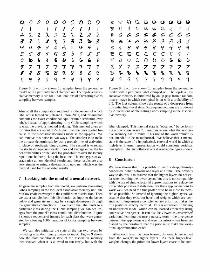
Figure 8: Each row shows 10 samples from the generativemodel with a particular label clamped on. The top-level asso-ciative memory is run for 1000 iterations of alternating Gibbssampling between samples.

Almost all the computation required is independent of whichlabel unit is turned on (Teh and Hinton, 2001) and this methodcomputes the exact conditional equilibrium distribution overlabels instead of approximating it by Gibbs sampling whichis what the previous method is doing. This method gives er-ror rates that are about 0.5% higher than the ones quoted be-cause of the stochastic decisions made in the up-pass. Wecan remove this noise in two ways. The simplest is to makethe up-pass deterministic by using probabilities of activationin place of stochastic binary states. The second is to repeatthe stochastic up-pass twenty times and average either the la-bel probabilities or the label log probabilities over the twentyrepetitions before picking the best one. The two types of av-erage give almost identical results and these results are alsovery similar to using a deterministic up-pass, which was themethod used for the reported results.

7 Looking into the mind of a neural network

To generate samples from the model, we perform alternatingGibbs sampling in the top-level associative memory until theMarkov chain converges to the equilibrium distribution. Thenwe use a sample from this distribution as input to the layersbelow and generate an image by a single down-pass throughthe generative connections. If we clamp the label units to aparticular class during the Gibbs sampling we can see im-ages from the model’s class-conditional distributions. Figure8 shows a sequence of images for each class that were gener-ated by allowing 1000 iterations of Gibbs sampling betweensamples.

We can also initialize the state of the top two layers byproviding a random binary image as input. Figure 9 showshow the class-conditional state of the associative memorythen evolves when it is allowed to run freely, but with the

Figure 9: Each row shows 10 samples from the generativemodel with a particular label clamped on. The top-level as-sociative memory is initialized by an up-pass from a randombinary image in which each pixel is on with a probability of0.5. The first column shows the results of a down-pass fromthis initial high-level state. Subsequent columns are producedby 20 iterations of alternating Gibbs sampling in the associa-tive memory.

label clamped. This internal state is “observed” by perform-ing a down-pass every 20 iterations to see what the associa-tive memory has in mind. This use of the word “mind” isnot intended to be metaphorical. We believe that a mentalstate is the state of a hypothetical, external world in which ahigh-level internal representation would constitute veridicalperception. That hypothetical world is what the figure shows.

8 Conclusion

We have shown that it is possible to learn a deep, densely-connected, belief network one layer at a time. The obviousway to do this is to assume that the higher layers do not ex-ist when learning the lower layers, but this is not compatiblewith the use of simple factorial approximations to replace theintractable posterior distribution. For these approximations towork well, we need the true posterior to be as close to facto-rial as possible. So instead of ignoring the higher layers, weassume that they exist but have tied weights which are con-strained to implement a complementary prior that makes thetrue posterior exactly factorial. This is equivalent to havingan undirected model which can be learned efficiently usingcontrastive divergence. It can also be viewed as constrainedvariational learning because a penalty term – the divergencebetween the approximate and true posteriors – has been re-placed by the constraint that the prior must make the varia-tional approximation exact.

After each layer has been learned, its weights are untiedfrom the weights in higher layers. As these higher-levelweights change, the priors for lower layers cease to be com-

plementary, so the true posterior distributions in lower layersare no longer factorial and the use of the transpose of the gen-erative weights for inference is no longer correct. Neverthe-less, we can use a variational bound to show that adapting thehigher-level weights improves the overall generative model.

To demonstrate the power of our fast, greedy learningalgorithm, we used it to initialize the weights for a muchslower fine-tuning algorithm that learns an excellent gener-ative model of digit images and their labels. It is not clearthat this is the best way to use the fast, greedy algorithm. Itmight be better to omit the fine-tuning and use the speed ofthe greedy algorithm to learn an ensemble of larger, deepernetworks or a much larger training set. The network in figure1 has about as many parameters as 0.002 cubic millimetersof mouse cortex (Horace Barlow, pers. comm.), and severalhundred networks of this complexity could fit within a sin-gle voxel of a high resolution fMRI scan. This suggests thatmuch bigger networks may be required to compete with hu-man shape recognition abilities.

Our current generative model is limited in many ways (Leeand Mumford, 2003). It is designed for images in which non-binary values can be treated as probabilities (which is not thecase for natural images); its use of top-down feedback duringperception is limited to the associative memory in the top twolayers; it does not have a systematic way of dealing with per-ceptual invariances; it assumes that segmentation has alreadybeen performed and it does not learn to sequentially attend tothe most informative parts of objects when discrimination isdifficult. It does, however, illustrate some of the major ad-vantages of generative models as compared to discriminativeones:

1. Generative models can learn low-level features with-out requiring feedback from the label and they canlearn many more parameters than discriminative mod-els without overfitting. In discriminative learning, eachtraining case only constrains the parameters by as manybits of information as are required to specify the label.For a generative model, each training case constrainsthe parameters by the number of bits required to spec-ify the input.

2. It is easy to see what the network has learned by gener-ating from its model.

3. It is possible to interpret the non-linear, distributed rep-resentations in the deep hidden layers by generating im-ages from them.

4. The superior classification performance of discrimina-tive learning methods only holds for domains in whichit is not possible to learn a good generative model. Thisset of domains is being eroded by Moore’s law.

AcknowledgmentsWe thank Peter Dayan, Zoubin Ghahramani, Yann Le Cun,Andriy Mnih, Radford Neal, Terry Sejnowski and MaxWelling for helpful discussions and the referees for greatlyimproving the manuscript. The research was supported by

NSERC, the Gatsby Charitable Foundation, CFI and OIT.GEH is a fellow of the Canadian Institute for Advanced Re-search and holds a Canada Research Chair in machine learn-ing.

References

Belongie, S., Malik, J., and Puzicha, J. (2002). Shape match-ing and object recognition using shape contexts. IEEETransactions on Pattern Analysis and Machine Intelli-gence, 24(4):509–522.

Carreira-Perpinan, M. A. and Hinton, G. E. (2005). On con-trastive divergence learning. In Artificial Intelligence andStatistics, 2005.

Decoste, D. and Schoelkopf, B. (2002). Training invariantsupport vector machines. Machine Learning, 46:161–190.

Freund, Y. (1995). Boosting a weak learning algorithm bymajority. Information and Computation, 12(2):256 – 285.

Friedman, J. and Stuetzle, W. (1981). Projection pursuit re-gression. Journal of the American Statistical Association,76:817–823.

Hinton, G. E. (2002). Training products of experts byminimizing contrastive divergence. Neural Computation,14(8):1711–1800.

Hinton, G. E., Dayan, P., Frey, B. J., and Neal, R. (1995). Thewake-sleep algorithm for self-organizing neural networks.Science, 268:1158–1161.

LeCun, Y., Bottou, L., and Haffner, P. (1998). Gradient-basedlearning applied to document recognition. Proceedings ofthe IEEE, 86(11):2278–2324.

Lee, T. S. and Mumford, D. (2003). Hierarchical bayesian in-ference in the visual cortex. Journal of the Optical Societyof America, A., 20:1434–1448.

Marks, T. K. and Movellan, J. R. (2001). Diffusion networks,product of experts, and factor analysis. In Proc. Int. Conf.on Independent Component Analysis, pages 481–485.

Mayraz, G. and Hinton, G. E. (2001). Recognizing hand-written digits using hierarchical products of experts. IEEETransactions on Pattern Analysis and Machine Intelli-gence, 24:189–197.

Neal, R. (1992). Connectionist learning of belief networks.Artificial Intelligence, 56:71–113.

Neal, R. M. and Hinton, G. E. (1998). A new view of theEM algorithm that justifies incremental, sparse and othervariants. In Jordan, M. I., editor, Learning in GraphicalModels, pages 355—368. Kluwer Academic Publishers.

Ning, F., Delhomme, D., LeCun, Y., Piano, F., Bottou, L.,and Barbano, P. (2005). Toward automatic phenotyping ofdeveloping embryos from videos. IEEE Transactions onImage Processing, 14(9):1360–1371.

Pearl, J. (1988). Probabilistic Inference in Intelligent Sys-tems: Networks of Plausible Inference. Morgan Kauf-mann, San Mateo, CA.

Roth, S. and Black, M. J. (2005). Fields of experts: A frame-work for learning image priors. In IEEE Conf. on Com-puter Vision and Pattern Recognition.

Sanger, T. D. (1989). Optimal unsupervised learning in asingle-layer linear feedforward neural. Neural Networks,2(6):459–473.

Simard, P. Y., Steinkraus, D., and Platt, J. (2003). Best prac-tice for convolutional neural networks applied to visualdocument analysis. In International Conference on Docu-ment Analysis and Recogntion (ICDAR), IEEE ComputerSociety, Los Alamitos, pages 958–962.

Teh, Y. and Hinton, G. E. (2001). Rate-coded restricted Boltz-mann machines for face recognition. In Advances in Neu-ral Information Processing Systems, volume 13.

Teh, Y., Welling, M., Osindero, S., and Hinton, G. E. (2003).Energy-based models for sparse overcomplete representa-tions. Journal of Machine Learning Research, 4:1235–1260.

Welling, M., Hinton, G., and Osindero, S. (2003). Learn-ing sparse topographic representations with products ofStudent-t distributions. In S. Becker, S. T. and Ober-mayer, K., editors, Advances in Neural Information Pro-cessing Systems 15, pages 1359–1366. MIT Press, Cam-bridge, MA.

Welling, M., Rosen-Zvi, M., and Hinton, G. E. (2005). Expo-nential family harmoniums with an application to informa-tion retrieval. In Advances in Neural Information Process-ing Systems 17, pages 1481–1488. MIT Press, Cambridge,MA.

9 Tables

Version of MNIST task Learning algorithm Test error %permutation-invariant Our generative model 1.25

784−>500−>500<−−>2000<−−>10permutation-invariant Support Vector Machine 1.4

degree 9 polynomial kernelpermutation-invariant Backprop 784−>500−>300−>10 1.51

cross-entropy & weight-decaypermutation-invariant Backprop 784−>800−>10 1.53

cross-entropy & early stoppingpermutation-invariant Backprop 784−>500−>150−>10 2.95

squared error & on-line updatespermutation-invariant Nearest Neighbor 2.8

All 60,000 examples & L3 normpermutation-invariant Nearest Neighbor 3.1

All 60,000 examples & L2 normpermutation-invariant Nearest Neighbor 4.0

20,000 examples & L3 normpermutation-invariant Nearest Neighbor 4.4

20,000 examples & L2 normunpermuted images Backprop 0.4

extra data from cross-entropy & early-stoppingelastic deformations convolutional neural net

unpermuted deskewed Virtual SVM 0.56images, extra data degree 9 polynomial kernelfrom 2 pixel transl.unpermuted images Shape-context features 0.63

hand-coded matchingunpermuted images Backprop in LeNet5 0.8

extra data from convolutional neural netaffine transformationsUnpermuted images Backprop in LeNet5 0.95

convolutional neural net

Table 1: The error rates of various learning algorithms on the MNIST digit recognition task. See text for details.

10 Appendix

A Complementary Priors

General complementarity

Consider a joint distribution over observables, x, and hidden variables, y. For a given likelihood function, P (x|y), we definethe corresponding family of complementary priors to be those distributions, P (y), for which the joint distribution, P (x,y) =P (x|y)P (y), leads to posteriors, P (y|x), that exactly factorise, i.e. leads to a posterior that can be expressed as P (y|x) =∏

j P (yj |x).

Not all functional forms of likelihood admit a complementary prior. In this appendix we will show that the following familyconstitutes all likelihood functions admitting a complementary prior:

P (x|y) =1

Ω(y)exp

∑

j

Φj(x, yj) + β(x)

= exp

∑

j

Φj(x, yj) + β(x) − log Ω(y)

(11)

where Ω is the normalisation term. For this assertion to hold we need to assume positivity of distributions: that both P (y) > 0and P (x|y) > 0 for every value of y and x. The corresponding family of complementary priors then assume the form:

P (y) =1C

exp

log Ω(y) +

∑j

αj(yj)

(12)

where C is a constant to ensure normalisation. This combination of functional forms leads to the following expression for thejoint:

P (x,y) =1C

exp

∑

j

Φj(x, yj) + β(x) +∑

j

αj(yj)

(13)

To prove our assertion, we need to show that every likelihood function of the form in Eq. 11 admits a complementaryprior, and also that complementarity implies the functional form in Eq. 11. Firstly, it can be directly verified that Eq. 12 is acomplementary prior for the likelihood functions of Eq. 11. To show the converse, let us assume that P (y) is a complementaryprior for some likelihood function P (x|y). Notice that the factorial form of the posterior simply means that the joint distributionP (x,y) = P (y)P (x|y) satisfies the following set of conditional independencies: yj ⊥⊥ yk |x for every j = k. This set ofconditional independencies is exactly those satisfied by an undirected graphical model with an edge between every hiddenvariable and observed variable and among all observed variables (Pearl, 1988). By the Hammersley-Clifford Theorem, andusing our positivity assumption, the joint distribution must be of the form of Eq. 13, and the forms for the likelihood functionEq. 11 and prior Eq. 12 follow from this.

Complementarity for infinite stacks

We now consider a subset of models of the form in Eq. 13 for which the likelihood also factorises. This means that we nowhave two sets of conditional independencies:

P (x|y) =∏

i

P (xi|y) (14)

P (y|x) =∏j

P (yj |x) (15)

This condition is useful for our construction of the infinite stack of directed graphical models.

Identifying the conditional independencies in Eq. 14 and 15 as those satisfied by a complete bipartite undirected graph-ical model, and again using the Hammersley-Clifford Theorem (assuming positivity), we see that the following form fully

characterises all joint distributions of interest,

P (x,y) =1Z

exp

∑

i,j

Ψi,j(xi, yj) +∑

i

γi(xi) +∑

j

αj(yj)

(16)

while the likelihood functions take on the form,

P (x|y) = exp

∑

i,j

Ψi,j(xi, yj) +∑

i

γi(xi) − log Ω(y)

(17)

Although it is not immediately obvious, the marginal distribution over the observables, x, in Eq. 16 can also be expressedas an infinite directed model in which the parameters defining the conditional distributions between layers are tied together.

An intuitive way of validating of this assertion is as follows. Consider one of the methods by which we might draw samplesfrom the marginal distribution P (x) implied by Eq. 16. Starting from an arbitrary configuration of y we would iterativelyperform Gibbs sampling using, in alternation, the distributions given in Eq. 14 and 15. If we run this Markov chain for longenough then, since our positivity assumptions ensure that the chain mixes properly, we will eventually obtain unbiased samplesfrom the joint distribution given in Eq. 16.

Now let us imagine that we unroll this sequence of Gibbs updates in space — such that we consider each parallel update ofthe variables to constitute states of a separate layer in a graph. This unrolled sequence of states has a purely directed structure(with conditional distributions taking the form of Eq. 14 and 15 in alternation). By equivalence to the Gibbs sampling scheme,after many layers in such an unrolled graph, adjacent pairs of layers will have a joint distribution as given in Eq. 16.

We can formalize this intuition for unrolling the graph as follows. The basic idea is to construct a joint distribution byunrolling a graph “upwards” (i.e. moving away from the data-layer to successively deeper hidden layers), so that we can put awell-defined distribution over an infinite stack of variables. Then we verify some simple marginal and conditional propertiesof this joint distribution, and show that our construction is the same as that obtained by unrolling the graph downwards from avery deep layer.

Let x = x(0),y = y(0),x(1),y(1),x(2),y(2), . . . be a sequence (stack) of variables the first two of which are identified asour original observed and hidden variables, while x(i) and y(i) are interpreted as a sequence of successively deeper layers.First, define the functions

f(x′,y′) =1Z

exp

∑

i,j

Ψi,j(x′i, y

′i) +

∑i

γi(x′i) +

∑j

αj(y′j)

(18)

fx(x′) =∑y′

f(x′,y′) (19)

fy(y′) =∑x′

f(x′,y′) (20)

gx(x′|y′) = f(x′,y′)/fy(y′) (21)

gy(y′|x′) = f(x′,y′)/fx(x′) (22)

over dummy variables y′, x′. Now define a joint distribution over our sequence of variables (assuming first-order Markoviandependency) as follows:

P (x(0),y(0)) = f(x(0),y(0)) (23)

P (x(i)|y(i−1)) = gx(x(i)|y(i−1)) i = 1, 2, . . . (24)

P (y(i)|x(i)) = gy(y(i)|x(i)) i = 1, 2, . . . (25)

We verify by induction that the distribution has the following marginal distributions:

P (x(i)) = fx(x(i)) i = 0, 1, 2, . . . (26)

P (y(i)) = fy(y(i)) i = 0, 1, 2, . . . (27)

For i = 0 this is given by definition of the distribution in Eq. 23 and by Eqs. 19 and 20. For i > 0, we have:

P (x(i)) =∑

y(i−1)

P (x(i)|y(i−1))P (y(i−1)) =∑

y(i−1)

f(x(i),y(i−1))fy(y(i−1))

fy(y(i−1)) = fx(x(i)) (28)

and similarly for P (y(i)). Now we see that the following “downward” conditional distributions also hold true:

P (x(i)|y(i)) = P (x(i),y(i))/P (y(i)) = gx(x(i)|y(i)) (29)

P (y(i)|x(i+1)) = P (y(i),x(i+1))/P (x(i+1)) = gy(y(i)|x(i+1)) (30)

So our joint distribution over the stack of variables also gives the unrolled graph in the “downward” direction, since the con-ditional distributions in Eq. 29 and 30 are the same as those used to generate a sample in a downwards pass and the Markovchain mixes.

Inference in this infinite stack of directed graphs is equivalent to inference in the joint distribution over the sequence ofvariables. In other words, given x(0) we can simply use the definition of the joint distribution Eqs. 23, 24 and 25 to obtaina sample from the posterior simply by sampling y(0)|x(0), x(1)|y(0), y(1)|x(1), . . .. This directly shows that our inferenceprocedure is exact for the unrolled graph.

B Pseudo-Code For Up-Down Algorithm

We now present “MATLAB-style” pseudo-code for an implementation of the up-down algorithm described in section 5 andused for back-fitting. (This method is a contrastive version of the wake-sleep algorithm (Hinton et al., 1995).)

The code outlined below assumes a network of the type shown in Figure 1 with visible inputs, label nodes, and three layersof hidden units. Before applying the up-down algorithm, we would first perform layer-wise greedy training as described insections 3 and 4.

\% UP-DOWN ALGORITHM\%\% the data and all biases are row vectors.\% the generative model is: lab <--> top <--> pen --> hid --> vis\% the number of units in layer foo is numfoo\% weight matrices have names fromlayer_tolayer\% "rec" is for recognition biases and "gen" is for generative biases.\% for simplicity, the same learning rate, r, is used everywhere.

\% PERFORM A BOTTOM-UP PASS TO GET WAKE/POSITIVE PHASE PROBABILITIES\% AND SAMPLE STATESwakehidprobs = logistic(data*vishid + hidrecbiases);wakehidstates = wakehidprobs > rand(1, numhid);wakepenprobs = logistic(wakehidstates*hidpen + penrecbiases);wakepenstates = wakepenprobs > rand(1, numpen);postopprobs = logistic(wakepenstates*pentop + targets*labtop + topbiases);postopstates = waketopprobs > rand(1, numtop));

\% POSITIVE PHASE STATISTICS FOR CONTRASTIVE DIVERGENCEposlabtopstatistics = targets’ * waketopstates;pospentopstatistics = wakepenstates’ * waketopstates;

\% PERFORM numCDiters GIBBS SAMPLING ITERATIONS USING THE TOP LEVEL\% UNDIRECTED ASSOCIATIVE MEMORYnegtopstates = waketopstates; \% to initialize loopfor iter=1:numCDiters

negpenprobs = logistic(negtopstates*pentop’ + pengenbiases);negpenstates = negpenprobs > rand(1, numpen);neglabprobs = softmax(negtopstates*labtop’ + labgenbiases);negtopprobs = logistic(negpenstates*pentop+neglabprobs*labtop+topbiases);negtopstates = negtopprobs > rand(1, numtop));

end;\% NEGATIVE PHASE STATISTICS FOR CONTRASTIVE DIVERGENCEnegpentopstatistics = negpenstates’*negtopstates;neglabtopstatistics = neglabprobs’*negtopstates;

\% STARTING FROM THE END OF THE GIBBS SAMPLING RUN, PERFORM A\% TOP-DOWN GENERATIVE PASS TO GET SLEEP/NEGATIVE PHASE PROBABILITIES\% AND SAMPLE STATESsleeppenstates = negpenstates;sleephidprobs = logistic(sleeppenstates*penhid + hidgenbiases);sleephidstates = sleephidprobs > rand(1, numhid);sleepvisprobs = logistic(sleephidstates*hidvis + visgenbiases);

\% PREDICTIONSpsleeppenstates = logistic(sleephidstates*hidpen + penrecbiases);psleephidstates = logistic(sleepvisprobs*vishid + hidrecbiases);pvisprobs = logistic(wakehidstates*hidvis + visgenbiases);phidprobs = logistic(wakepenstates*penhid + hidgenbiases);

\% UPDATES TO GENERATIVE PARAMETERS-hidvis = hidvis + r*poshidstates’*(data-pvisprobs);visgenbiases = visgenbiases + r*(data - pvisprobs);penhid = penhid + r*wakepenstates’*(wakehidstates-phidprobs);hidgenbiases = hidgenbiases + r*(wakehidstates - phidprobs);

\% UPDATES TO TOP LEVEL ASSOCIATIVE MEMORY PARAMETERSlabtop = labtop + r*(poslabtopstatistics-neglabtopstatistics);labgenbiases = labgenbiases + r*(targets - neglabprobs);pentop = pentop + r*(pospentopstatistics - negpentopstatistics);pengenbiases = pengenbiases + r*(wakepenstates - negpenstates);topbiases = topbiases + r*(waketopsates - negtopstates);

\%UPDATES TO RECOGNITION/INFERENCE APPROXIMATION PARAMETERShidpen = hidpen + r*(sleephidstates’*(sleeppenstates-psleeppenstates));penrecbiases = penrecbiases + r*(sleeppenstates-psleeppenstates);vishid = vishid + r*(sleepvisprobs’*(sleephidstates-psleephidstates));hidrecbiases = hidrecbiases + r*(sleephidstates-psleephidstates);