2007 NIPS Tutorial on:

Deep Belief NetsGeoffrey Hinton

Canadian Institute for Advanced Research&

Department of Computer ScienceUniversity of Toronto

Some things you will learn in this tutorial

• How to learn multi-layer generative models of unlabelleddata by learning one layer of features at a time.– How to add Markov Random Fields in each hidden layer.

• How to use generative models to make discriminativetraining methods work much better for classification andregression.– How to extend this approach to Gaussian Processes and

how to learn complex, domain-specific kernels for aGaussian Process.

• How to perform non-linear dimensionality reduction on verylarge datasets– How to learn binary, low-dimensional codes and how to

use them for very fast document retrieval.• How to learn multilayer generative models of high-

dimensional sequential data.

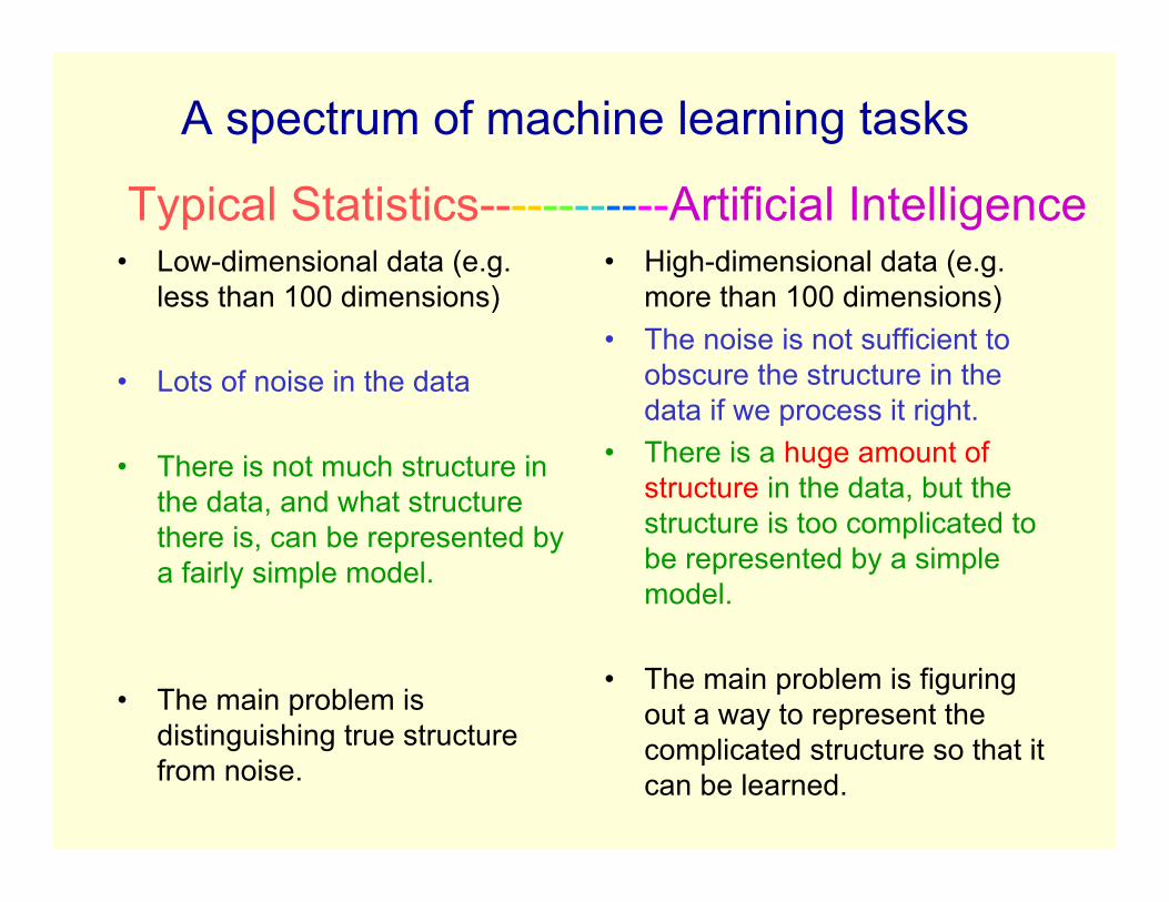
A spectrum of machine learning tasks

• Low-dimensional data (e.g.less than 100 dimensions)

• Lots of noise in the data

• There is not much structure inthe data, and what structurethere is, can be represented bya fairly simple model.

• The main problem isdistinguishing true structurefrom noise.

• High-dimensional data (e.g.more than 100 dimensions)

• The noise is not sufficient toobscure the structure in thedata if we process it right.

• There is a huge amount ofstructure in the data, but thestructure is too complicated tobe represented by a simplemodel.

• The main problem is figuringout a way to represent thecomplicated structure so that itcan be learned.

Typical Statistics------------Artificial Intelligence

Historical background:First generation neural networks

• Perceptrons (~1960)used a layer of hand-coded features and triedto recognize objects bylearning how to weightthese features.– There was a neat

learning algorithm foradjusting the weights.

– But perceptrons arefundamentally limitedin what they can learnto do.

non-adaptivehand-codedfeatures

output unitse.g. class labels

input unitse.g. pixels

Sketch of a typicalperceptron from the 1960’s

Bomb Toy

Second generation neural networks (~1985)

input vector

hiddenlayers

outputs

Back-propagateerror signal toget derivativesfor learning

Compare outputs withcorrect answer to geterror signal

A temporary digression

• Vapnik and his co-workers developed a very clever typeof perceptron called a Support Vector Machine.– Instead of hand-coding the layer of non-adaptive

features, each training example is used to create anew feature using a fixed recipe.

• The feature computes how similar a test example is to thattraining example.

– Then a clever optimization technique is used to selectthe best subset of the features and to decide how toweight each feature when classifying a test case.

• But its just a perceptron and has all the same limitations.

• In the 1990’s, many researchers abandoned neuralnetworks with multiple adaptive hidden layers becauseSupport Vector Machines worked better.

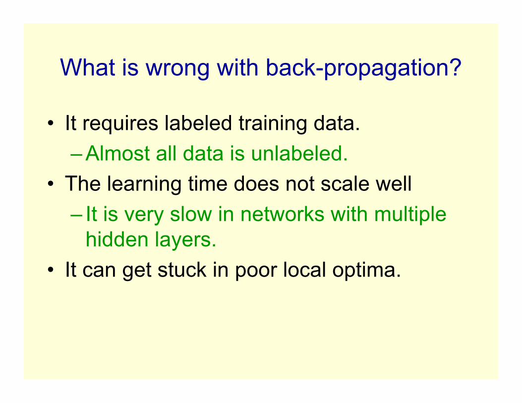
What is wrong with back-propagation?

• It requires labeled training data.– Almost all data is unlabeled.

• The learning time does not scale well– It is very slow in networks with multiple

hidden layers.• It can get stuck in poor local optima.

Overcoming the limitations of back-propagation

• Keep the efficiency and simplicity of using agradient method for adjusting the weights, but useit for modeling the structure of the sensory input.– Adjust the weights to maximize the probability

that a generative model would have producedthe sensory input.

– Learn p(image) not p(label | image)• If you want to do computer vision, first learn

computer graphics• What kind of generative model should we learn?

Belief Nets• A belief net is a directed

acyclic graph composed ofstochastic variables.

• We get to observe some ofthe variables and we wouldlike to solve two problems:

• The inference problem: Inferthe states of the unobservedvariables.

• The learning problem: Adjustthe interactions betweenvariables to make thenetwork more likely togenerate the observed data.

stochastichiddencause

visible effect

We will use nets composed oflayers of stochastic binary variableswith weighted connections. Later,we will generalize to other types ofvariable.

Stochastic binary units(Bernoulli variables)

• These have a state of 1or 0.

• The probability ofturning on is determinedby the weighted inputfrom other units (plus abias)

00

1

!""+==

j

jijii

wsbsp

)exp(1)(

11

!+j

jiji wsb

)( 1=isp

Learning Deep Belief Nets• It is easy to generate an

unbiased example at theleaf nodes, so we can seewhat kinds of data thenetwork believes in.

• It is hard to infer theposterior distribution overall possible configurationsof hidden causes.

• It is hard to even get asample from the posterior.

• So how can we learn deepbelief nets that havemillions of parameters?

stochastichiddencause

visible effect

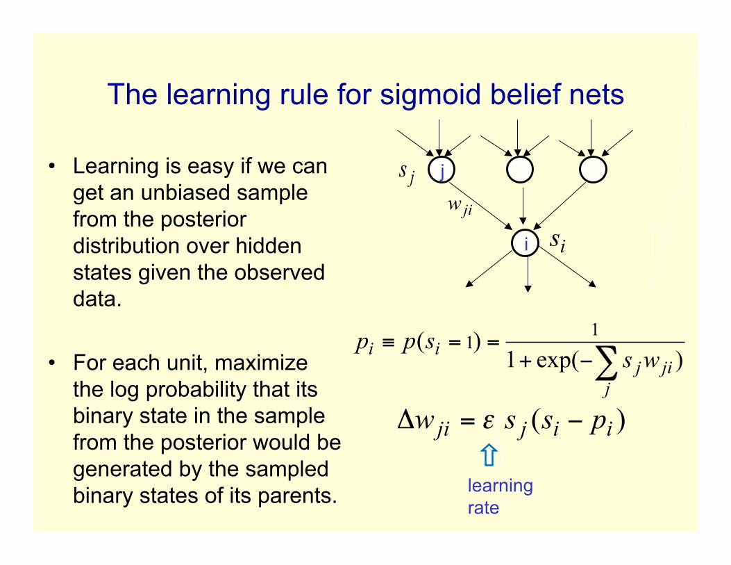
The learning rule for sigmoid belief nets

• Learning is easy if we canget an unbiased samplefrom the posteriordistribution over hiddenstates given the observeddata.

• For each unit, maximizethe log probability that itsbinary state in the samplefrom the posterior would begenerated by the sampledbinary states of its parents.

!"+==#

j

jijii

wsspp

)exp(1)(

11

j

i

jiw

)( iijji pssw !=" #

is

js

learningrate

Explaining away (Judea Pearl)

• Even if two hidden causes are independent, they canbecome dependent when we observe an effect that they canboth influence.– If we learn that there was an earthquake it reduces the

probability that the house jumped because of a truck.

truck hits house earthquake

house jumps

20 20

-20

-10 -10

p(1,1)=.0001p(1,0)=.4999p(0,1)=.4999p(0,0)=.0001

posterior

Why it is usually very hard to learnsigmoid belief nets one layer at a time

• To learn W, we need the posteriordistribution in the first hidden layer.

• Problem 1: The posterior is typicallycomplicated because of “explainingaway”.

• Problem 2: The posterior dependson the prior as well as the likelihood.– So to learn W, we need to know

the weights in higher layers, evenif we are only approximating theposterior. All the weights interact.

• Problem 3: We need to integrateover all possible configurations ofthe higher variables to get the priorfor first hidden layer. Yuk!

data

hidden variables

hidden variables

hidden variables

likelihood W

prior

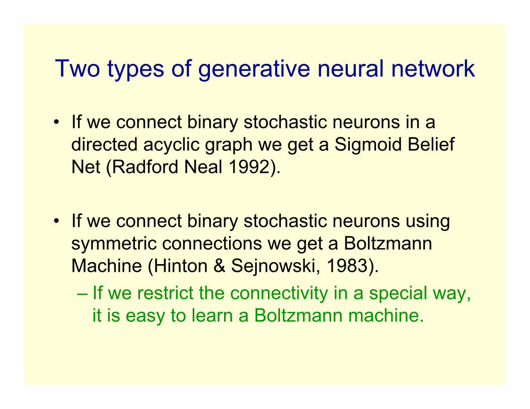
Two types of generative neural network

• If we connect binary stochastic neurons in adirected acyclic graph we get a Sigmoid BeliefNet (Radford Neal 1992).

• If we connect binary stochastic neurons usingsymmetric connections we get a BoltzmannMachine (Hinton & Sejnowski, 1983).– If we restrict the connectivity in a special way,

it is easy to learn a Boltzmann machine.

Restricted Boltzmann Machines(Smolensky ,1986, called them “harmoniums”)

• We restrict the connectivity to makelearning easier.– Only one layer of hidden units.

• We will deal with more layers later

– No connections between hidden units.• In an RBM, the hidden units are

conditionally independent given thevisible states.– So we can quickly get an unbiased

sample from the posterior distributionwhen given a data-vector.

– This is a big advantage over directedbelief nets

hidden

i

j

visible

The Energy of a joint configuration(ignoring terms to do with biases)

!"=

ji

ijji whvv,hE,

)(

weight betweenunits i and j

Energy with configurationv on the visible units andh on the hidden units

binary state ofvisible unit i

binary state ofhidden unit j

ji

ij

hvw

hvE=

!

!"

),(

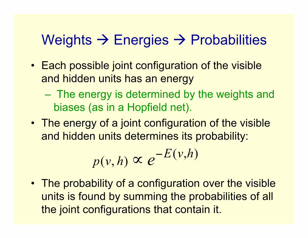
Weights Energies Probabilities

• Each possible joint configuration of the visibleand hidden units has an energy– The energy is determined by the weights and

biases (as in a Hopfield net).• The energy of a joint configuration of the visible

and hidden units determines its probability:

• The probability of a configuration over the visibleunits is found by summing the probabilities of allthe joint configurations that contain it.

),(),(

hvEhvp e!"

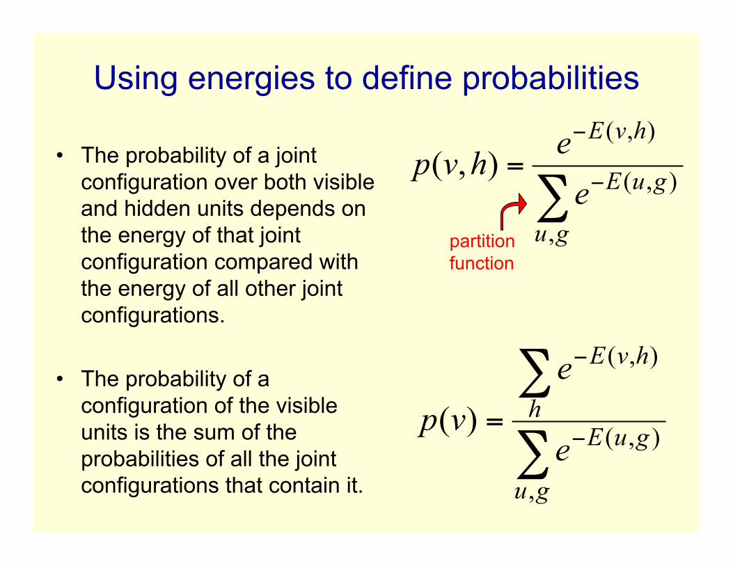
Using energies to define probabilities

• The probability of a jointconfiguration over both visibleand hidden units depends onthe energy of that jointconfiguration compared withthe energy of all other jointconfigurations.

• The probability of aconfiguration of the visibleunits is the sum of theprobabilities of all the jointconfigurations that contain it.

! "

"

=

gu

guE

hvE

e

ehvp

,

),(

),(

),(

!

!"

"

=

gu

guEh

hvE

e

e

vp

,

),(

),(

)(

partitionfunction

A picture of the maximum likelihood learningalgorithm for an RBM

0>< jihv

!>< jihv

i

j

i

j

i

j

i

j

t = 0 t = 1 t = 2 t = infinity

!><"><=

#

#jiji

ij

hvhvw

vp 0)(log

Start with a training vector on the visible units.

Then alternate between updating all the hidden units inparallel and updating all the visible units in parallel.

a fantasy

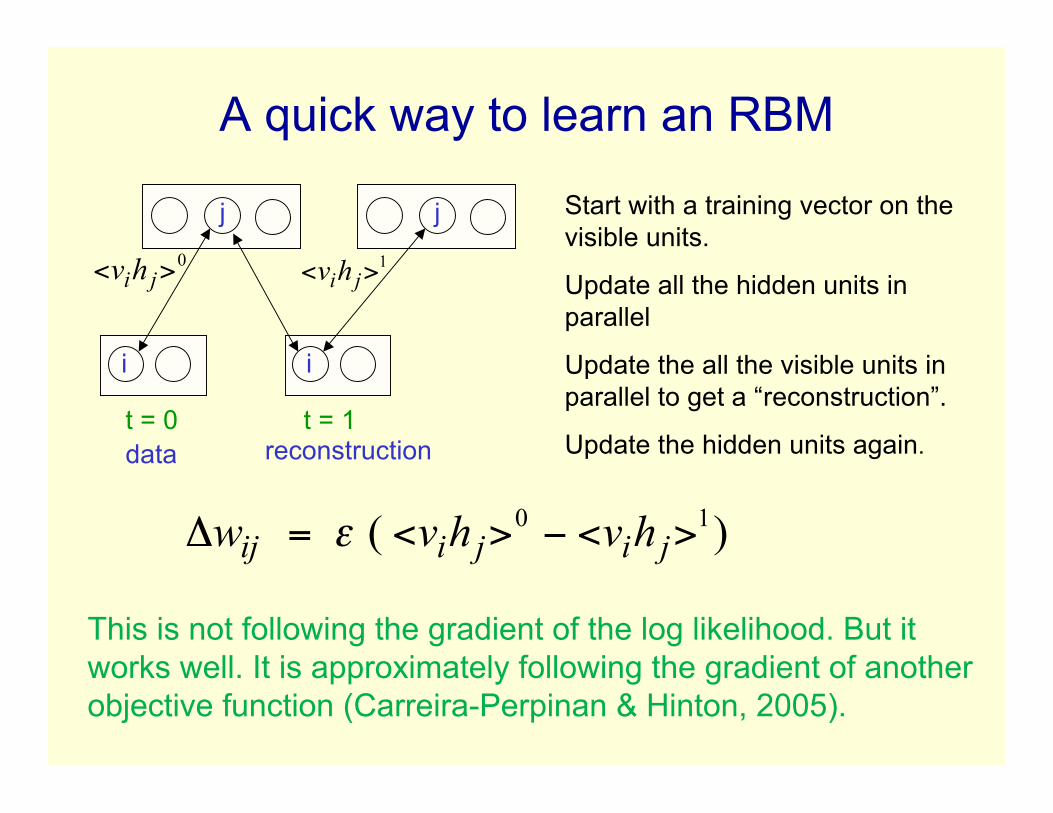
A quick way to learn an RBM

0>< jihv

1>< jihv

i

j

i

j

t = 0 t = 1

)( 10><!><=" jijiij hvhvw #

Start with a training vector on thevisible units.

Update all the hidden units inparallel

Update the all the visible units inparallel to get a “reconstruction”.

Update the hidden units again.

This is not following the gradient of the log likelihood. But itworks well. It is approximately following the gradient of anotherobjective function (Carreira-Perpinan & Hinton, 2005).

reconstructiondata

How to learn a set of features that are good forreconstructing images of the digit 2

50 binaryfeatureneurons

16 x 16pixelimage

50 binaryfeatureneurons

16 x 16pixelimage

Increment weightsbetween an activepixel and an activefeature

Decrement weightsbetween an activepixel and an activefeature

data(reality)

reconstruction(better than reality)

The final 50 x 256 weights

Each neuron grabs a different feature.

Reconstructionfrom activatedbinary featuresData

Reconstructionfrom activatedbinary featuresData

How well can we reconstruct the digit imagesfrom the binary feature activations?

New test images fromthe digit class that themodel was trained on

Images from anunfamiliar digit class(the network tries to seeevery image as a 2)

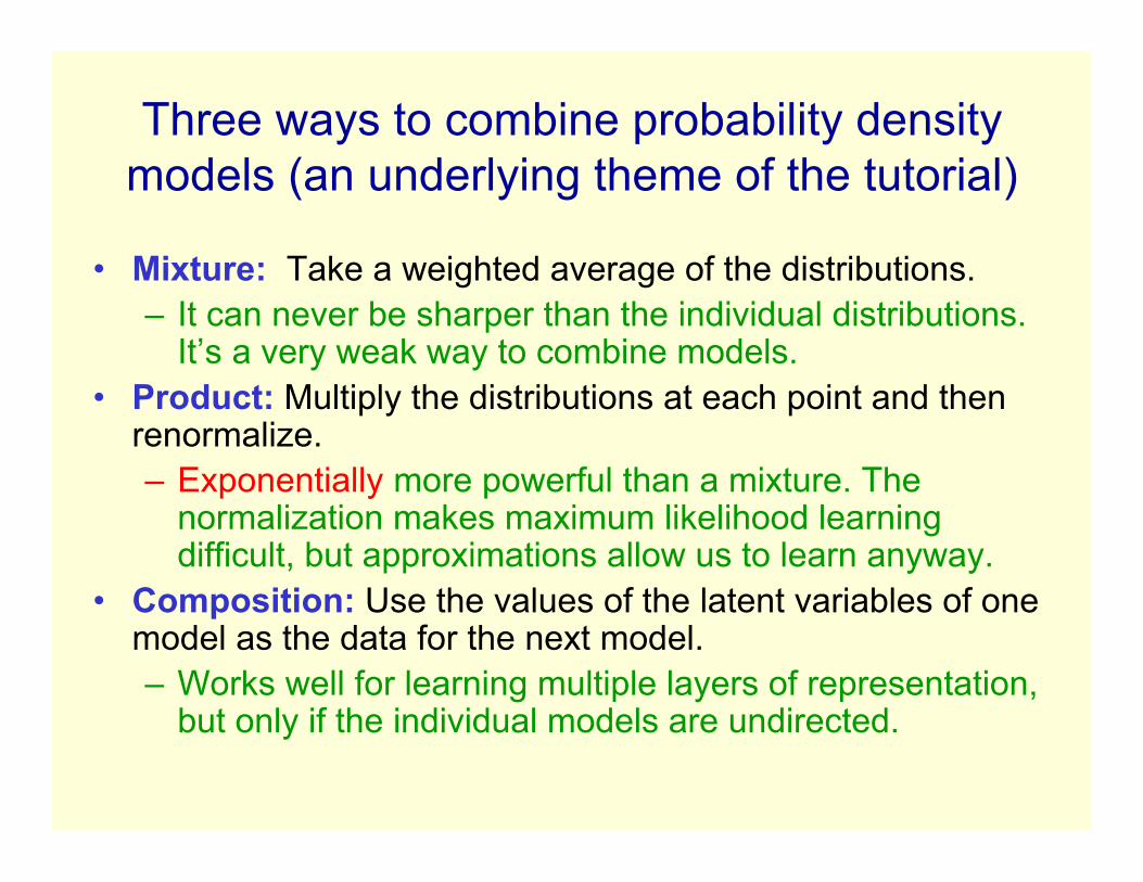
Three ways to combine probability densitymodels (an underlying theme of the tutorial)

• Mixture: Take a weighted average of the distributions.– It can never be sharper than the individual distributions.

It’s a very weak way to combine models.• Product: Multiply the distributions at each point and then

renormalize.– Exponentially more powerful than a mixture. The

normalization makes maximum likelihood learningdifficult, but approximations allow us to learn anyway.

• Composition: Use the values of the latent variables of onemodel as the data for the next model.– Works well for learning multiple layers of representation,

but only if the individual models are undirected.

Training a deep network(the main reason RBM’s are interesting)

• First train a layer of features that receive input directlyfrom the pixels.

• Then treat the activations of the trained features as ifthey were pixels and learn features of features in asecond hidden layer.

• It can be proved that each time we add another layer offeatures we improve a variational lower bound on the logprobability of the training data.– The proof is slightly complicated.– But it is based on a neat equivalence between an

RBM and a deep directed model (described later)

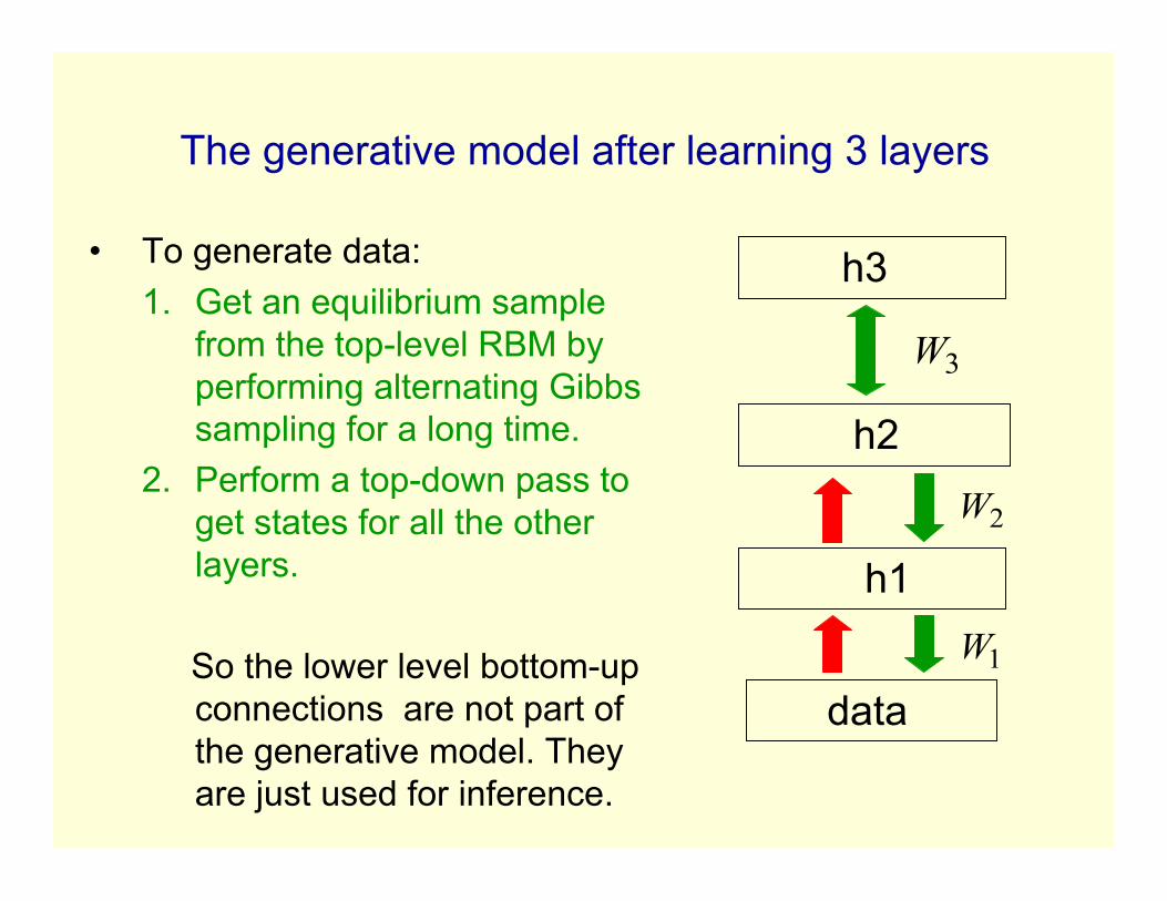
The generative model after learning 3 layers

• To generate data:1. Get an equilibrium sample

from the top-level RBM byperforming alternating Gibbssampling for a long time.

2. Perform a top-down pass toget states for all the otherlayers.

So the lower level bottom-upconnections are not part ofthe generative model. Theyare just used for inference.

h2

data

h1

h3

2W

3W

1W

Why does greedy learning work?An aside: Averaging factorial distributions

• If you average some factorial distributions, youdo NOT get a factorial distribution.– In an RBM, the posterior over the hidden units

is factorial for each visible vector.– But the aggregated posterior over all training

cases is not factorial (even if the data wasgenerated by the RBM itself).

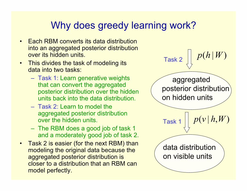
Why does greedy learning work?• Each RBM converts its data distribution

into an aggregated posterior distributionover its hidden units.

• This divides the task of modeling itsdata into two tasks:– Task 1: Learn generative weights

that can convert the aggregatedposterior distribution over the hiddenunits back into the data distribution.

– Task 2: Learn to model theaggregated posterior distributionover the hidden units.

– The RBM does a good job of task 1and a moderately good job of task 2.

• Task 2 is easier (for the next RBM) thanmodeling the original data because theaggregated posterior distribution iscloser to a distribution that an RBM canmodel perfectly.

data distributionon visible units

aggregatedposterior distributionon hidden units

)|( Whp

),|( Whvp

Task 2

Task 1

Why does greedy learning work?

!=h

hvphpvp )|()()(

The weights, W, in the bottom level RBM definep(v|h) and they also, indirectly, define p(h).

So we can express the RBM model as

If we leave p(v|h) alone and improve p(h), we willimprove p(v).

To improve p(h), we need it to be a better model ofthe aggregated posterior distribution over hiddenvectors produced by applying W to the data.

Which distributions are factorial in adirected belief net?

• In a directed belief net with one hidden layer, theposterior over the hidden units for each visiblevector is non-factorial (due to explaining away).– The aggregated posterior is factorial if the

data was generated by the directed model.• It’s the opposite way round from an undirected

model.• The intuitions that people have from using directed

models are very misleading for undirected models.

Why does greedy learning fail in a directed module?

• A directed module also converts its datadistribution into an aggregated posterior– Task 1 is now harder because the

posterior for each training case is non-factorial.

– Task 2 is performed using anindependent prior. This is a badapproximation unless the aggregatedposterior is close to factorial.

• A directed module attempts to make theaggregated posterior factorial in one step.– This is too difficult and leads to a bad

compromise. There is no guaranteethat the aggregated posterior is easierto model than the data distribution.

data distributionon visible units

)|( 2Whp

),|( 1Whvp

Task 2

Task 1

aggregatedposterior distributionon hidden units

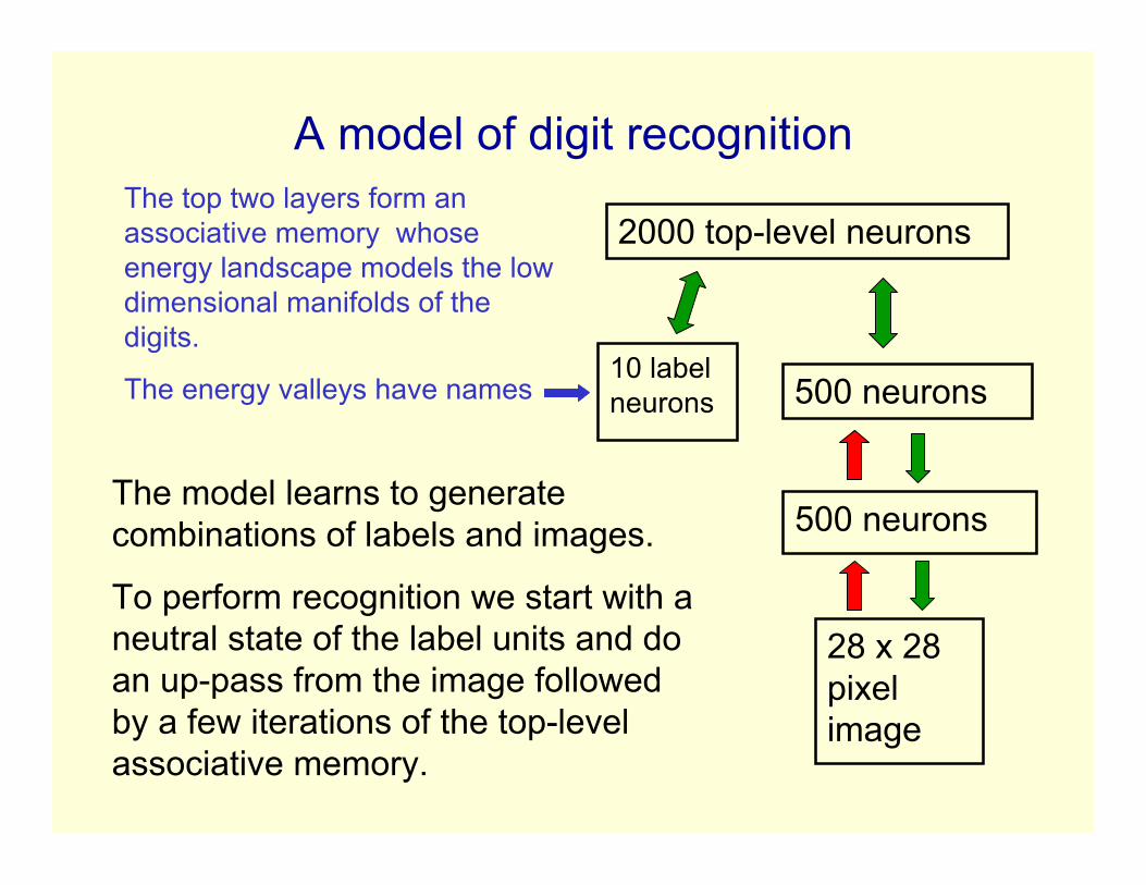
A model of digit recognition

2000 top-level neurons

500 neurons

500 neurons

28 x 28pixelimage

10 labelneurons

The model learns to generatecombinations of labels and images.

To perform recognition we start with aneutral state of the label units and doan up-pass from the image followedby a few iterations of the top-levelassociative memory.

The top two layers form anassociative memory whoseenergy landscape models the lowdimensional manifolds of thedigits.

The energy valleys have names

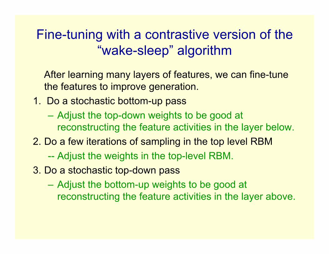
Fine-tuning with a contrastive version of the“wake-sleep” algorithm

After learning many layers of features, we can fine-tunethe features to improve generation.

1. Do a stochastic bottom-up pass– Adjust the top-down weights to be good at

reconstructing the feature activities in the layer below.2. Do a few iterations of sampling in the top level RBM

-- Adjust the weights in the top-level RBM.3. Do a stochastic top-down pass

– Adjust the bottom-up weights to be good atreconstructing the feature activities in the layer above.

Show the movie of the networkgenerating digits

(available at www.cs.toronto/~hinton)

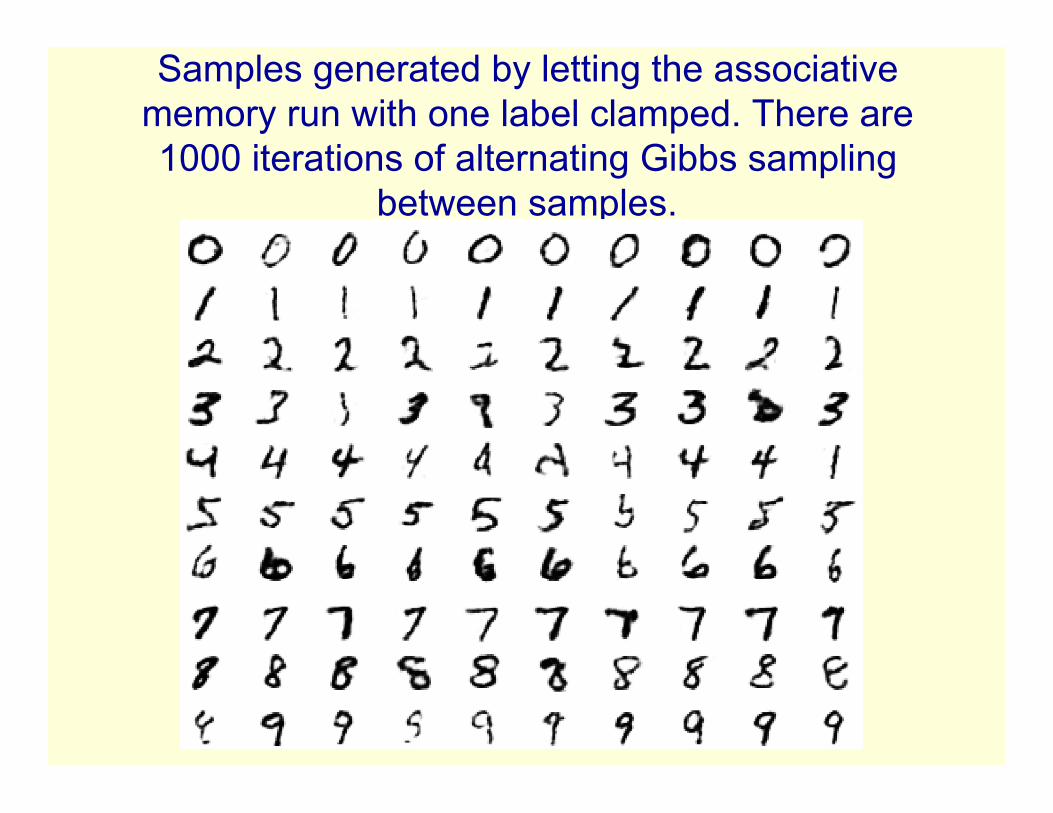
Samples generated by letting the associativememory run with one label clamped. There are1000 iterations of alternating Gibbs sampling

between samples.

Examples of correctly recognized handwritten digitsthat the neural network had never seen before

Its verygood

How well does it discriminate on MNIST test set withno extra information about geometric distortions?

• Generative model based on RBM’s 1.25%• Support Vector Machine (Decoste et. al.) 1.4%• Backprop with 1000 hiddens (Platt) ~1.6%• Backprop with 500 -->300 hiddens ~1.6%• K-Nearest Neighbor ~ 3.3%• See Le Cun et. al. 1998 for more results

• Its better than backprop and much more neurally plausiblebecause the neurons only need to send one kind of signal,and the teacher can be another sensory input.

Unsupervised “pre-training” also helps formodels that have more data and better priors

• Ranzato et. al. (NIPS 2006) used an additional600,000 distorted digits.

• They also used convolutional multilayer neuralnetworks that have some built-in, localtranslational invariance.

Back-propagation alone: 0.49%

Unsupervised layer-by-layerpre-training followed by backprop: 0.39% (record)

Another view of why layer-by-layerlearning works

• There is an unexpected equivalence betweenRBM’s and directed networks with many layersthat all use the same weights.– This equivalence also gives insight into why

contrastive divergence learning works.

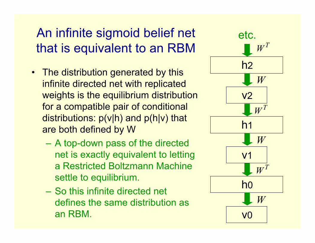
An infinite sigmoid belief netthat is equivalent to an RBM

• The distribution generated by thisinfinite directed net with replicatedweights is the equilibrium distributionfor a compatible pair of conditionaldistributions: p(v|h) and p(h|v) thatare both defined by W– A top-down pass of the directed

net is exactly equivalent to lettinga Restricted Boltzmann Machinesettle to equilibrium.

– So this infinite directed netdefines the same distribution asan RBM.

W

v1

h1

v0

h0

v2

h2

TW

TW

TW

W

W

etc.

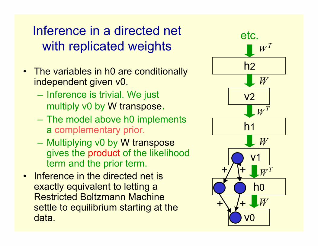
• The variables in h0 are conditionallyindependent given v0.– Inference is trivial. We just

multiply v0 by W transpose.– The model above h0 implements

a complementary prior.– Multiplying v0 by W transpose

gives the product of the likelihoodterm and the prior term.

• Inference in the directed net isexactly equivalent to letting aRestricted Boltzmann Machinesettle to equilibrium starting at thedata.

Inference in a directed netwith replicated weights

W

v1

h1

v0

h0

v2

h2

TW

TW

TW

W

W

etc.

+

+

+

+

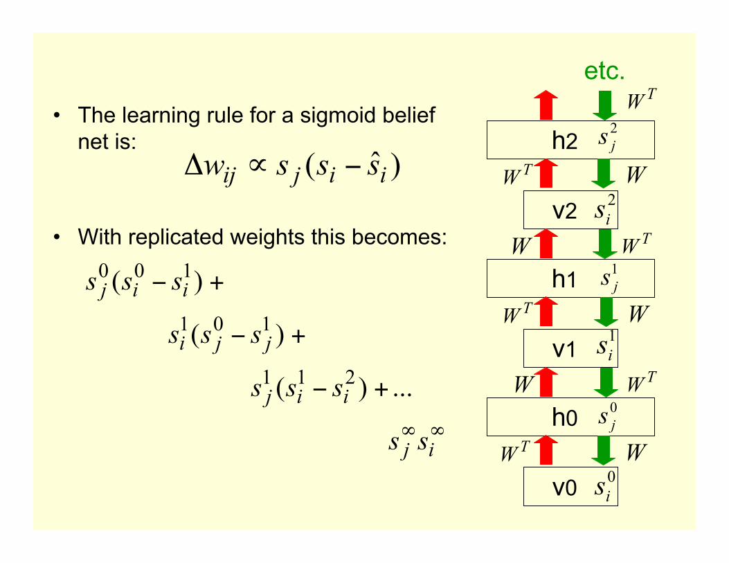
• The learning rule for a sigmoid beliefnet is:

• With replicated weights this becomes:

W

v1

h1

v0

h0

v2

h2

TW

TW

TW

W

W

etc.

0

is

0

js

1

js

2

js

1

is

2

is

!!

+"

+"

+"

ij

iij

jji

iij

ss

sss

sss

sss

...)(

)(

)(

211

101

100

TW

TW

TW

W

W

)ˆ( iijij sssw !"#

• First learn with all the weights tied– This is exactly equivalent to

learning an RBM– Contrastive divergence learning

is equivalent to ignoring the smallderivatives contributed by the tiedweights between deeper layers.

Learning a deep directednetwork

W

W

v1

h1

v0

h0

v2

h2

TW

TW

TW

W

etc.

v0

h0

W

• Then freeze the first layer of weightsin both directions and learn theremaining weights (still tiedtogether).– This is equivalent to learning

another RBM, using theaggregated posterior distributionof h0 as the data.

W

v1

h1

v0

h0

v2

h2

TW

TW

TW

W

etc.

frozenW

v1

h0

W

TfrozenW

How many layers should we use and howwide should they be?

(I am indebted to Karl Rove for this slide)

• How many lines of code should an AI program use and howlong should each line be?– This is obviously a silly question.

• Deep belief nets give the creator a lot of freedom.– How best to make use of that freedom depends on the

task.– With enough narrow layers we can model any distribution

over binary vectors (Sutskever & Hinton, 2007)• If freedom scares you, stick to convex optimization of

shallow models that are obviously inadequate for doingArtificial Intelligence.

What happens when the weights in higher layersbecome different from the weights in the first layer?

• The higher layers no longer implement a complementaryprior.– So performing inference using the frozen weights in

the first layer is no longer correct.– Using this incorrect inference procedure gives a

variational lower bound on the log probability of thedata.

• We lose by the slackness of the bound.

• The higher layers learn a prior that is closer to theaggregated posterior distribution of the first hidden layer.– This improves the network’s model of the data.

• Hinton, Osindero and Teh (2006) prove that thisimprovement is always bigger than the loss.

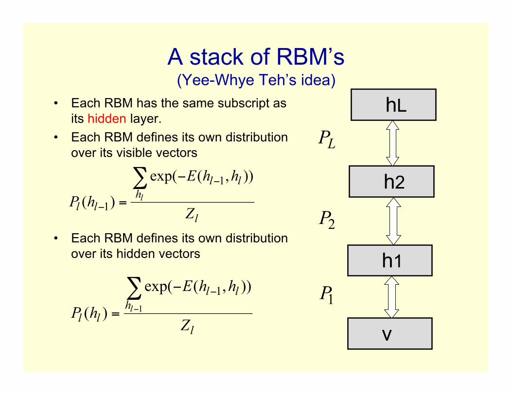
A stack of RBM’s(Yee-Whye Teh’s idea)

• Each RBM has the same subscript asits hidden layer.

• Each RBM defines its own distributionover its visible vectors

• Each RBM defines its own distributionover its hidden vectors

v

h1

h2

hL

1P

2P

LP

l

h

ll

llZ

hhE

hPl

! "

"

"

=

)),(exp(

)(

1

1

l

h

ll

llZ

hhE

hPl

!"

""

= 1

)),(exp(

)(

1

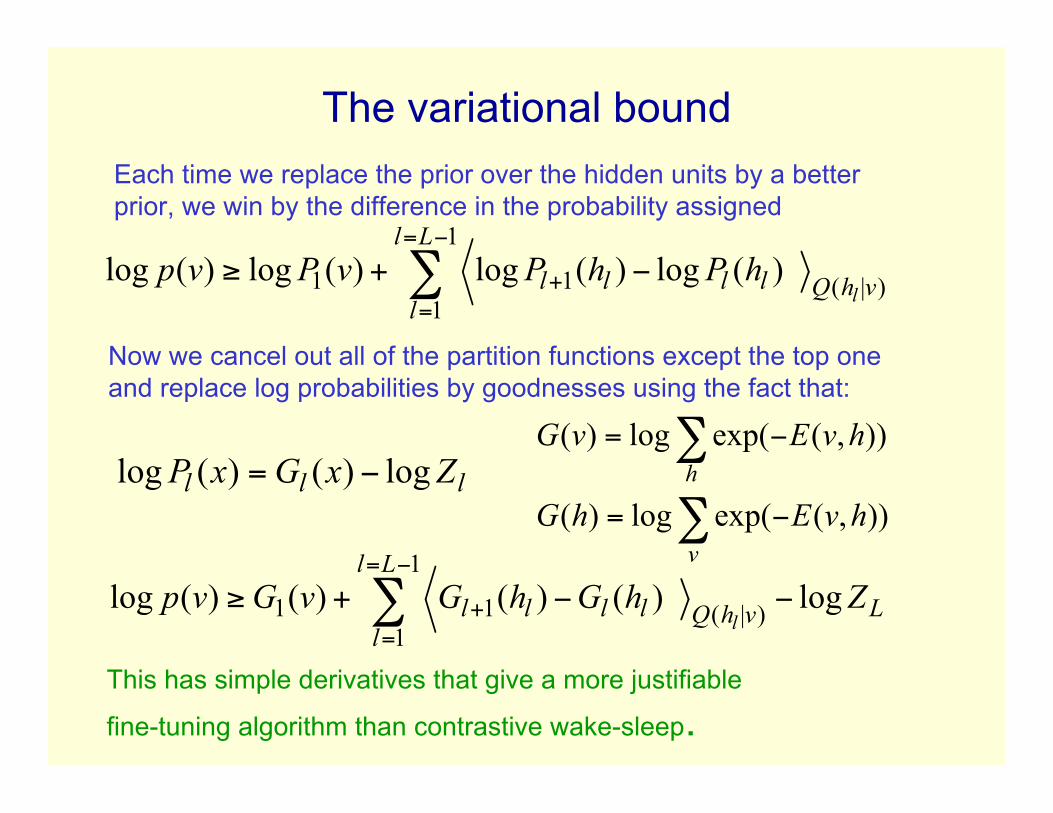
The variational bound

!"=

=

+ "+#1

1)|(11 )(log)(log)(log)(log

Ll

lvhQlllll

hPhPvPvp

L

Ll

lvhQllll ZhGhGvGvpl

log)()()()(log1

1)|(11 !!+" #

!=

=

+

Now we cancel out all of the partition functions except the top oneand replace log probabilities by goodnesses using the fact that:

This has simple derivatives that give a more justifiable

fine-tuning algorithm than contrastive wake-sleep.

lll ZxGxP log)()(log !=

Each time we replace the prior over the hidden units by a betterprior, we win by the difference in the probability assigned

!

!

"=

"=

v

h

hvEhG

hvEvG

)),(exp(log)(

)),(exp(log)(

Summary so far

• Restricted Boltzmann Machines provide a simple way tolearn a layer of features without any supervision.– Maximum likelihood learning is computationally

expensive because of the normalization term, butcontrastive divergence learning is fast and usuallyworks well.

• Many layers of representation can be learned by treatingthe hidden states of one RBM as the visible data fortraining the next RBM (a composition of experts).

• This creates good generative models that can then befine-tuned.– Contrastive wake-sleep can fine-tune generation.

Overview of the rest of the tutorial• How to fine-tune a greedily trained generative model to

be better at discrimination.

• How to learn a kernel for a Gaussian process.

• How to use deep belief nets for non-linear dimensionalityreduction and document retrieval.

• How to use deep belief nets for sequential data.

• How to learn a generative hierarchy of conditionalrandom fields.

BREAK

Fine-tuning for discrimination

• First learn one layer at a time greedily.• Then treat this as “pre-training” that finds a good

initial set of weights which can be fine-tuned bya local search procedure.– Contrastive wake-sleep is one way of fine-

tuning the model to be better at generation.• Backpropagation can be used to fine-tune the

model for better discrimination.– This overcomes many of the limitations of

standard backpropagation.

Why backpropagation works better aftergreedy pre-training

• Greedily learning one layer at a time scales well to reallybig networks, especially if we have locality in each layer.

• We do not start backpropagation until we already havesensible weights that already do well at the task.– So the initial gradients are sensible and backprop only

needs to perform a local search.• Most of the information in the final weights comes from

modeling the distribution of input vectors.– The precious information in the labels is only used for

the final fine-tuning. It slightly modifies the features. Itdoes not need to discover features.

– This type of backpropagation works well even if most ofthe training data is unlabeled. The unlabeled data isstill very useful for discovering good features.

First, model the distribution of digit images

2000 units

500 units

500 units

28 x 28pixelimage

The network learns a density model forunlabeled digit images. When we generatefrom the model we get things that look likereal digits of all classes.

But do the hidden features really help withdigit discrimination?

Add 10 softmaxed units to the top and dobackpropagation.

The top two layers form a restrictedBoltzmann machine whose free energylandscape should model the lowdimensional manifolds of the digits.

Results on permutation-invariant MNIST task

• Very carefully trained backprop net with 1.6%one or two hidden layers (Platt; Hinton)

• SVM (Decoste & Schoelkopf, 2002) 1.4%

• Generative model of joint density of 1.25%images and labels (+ generative fine-tuning)

• Generative model of unlabelled digits 1.15%followed by gentle backpropagation(Hinton & Salakhutdinov, Science 2006)

Combining deep belief nets with Gaussian processes

• Deep belief nets can benefit a lot from unlabeled datawhen labeled data is scarce.– They just use the labeled data for fine-tuning.

• Kernel methods, like Gaussian processes, work well onsmall labeled training sets but are slow for large trainingsets.

• So when there is a lot of unlabeled data and only a littlelabeled data, combine the two approaches:– First learn a deep belief net without using the labels.– Then apply Gaussian process models to the deepest

layer of features. This works better than using the rawdata.

– Then use GP’s to get the derivatives that are back-propagated through the deep belief net. This is afurther win. It allows GP’s to fine-tune complicateddomain-specific kernels.

Learning to extract the orientation of a face patch(Salakhutdinov & Hinton, NIPS 2007)

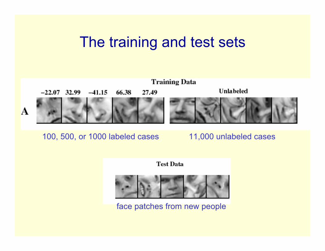
The training and test sets

11,000 unlabeled cases100, 500, or 1000 labeled cases

face patches from new people

The root mean squared error in the orientationwhen combining GP’s with deep belief nets

22.2 17.9 15.2

17.2 12.7 7.2

16.3 11.2 6.4

GP onthepixels

GP ontop-levelfeatures

GP on top-levelfeatures withfine-tuning

100 labels

500 labels

1000 labels

Conclusion: The deep features are much betterthan the pixels. Fine-tuning helps a lot.

Modeling real-valued data

• For images of digits it is possible to representintermediate intensities as if they were probabilities byusing “mean-field” logistic units.– We can treat intermediate values as the probability

that the pixel is inked.• This will not work for real images.

– In a real image, the intensity of a pixel is almostalways almost exactly the average of the neighboringpixels.

– Mean-field logistic units cannot represent preciseintermediate values.

The free-energy of a mean-field logistic unit

• In a mean-field logistic unit, thetotal input provides a linearenergy-gradient and the negativeentropy provides a containmentfunction with fixed curvature.

• So it is impossible for the value0.7 to have much lower freeenergy than both 0.8 and 0.6.This is no good for modelingreal-valued data.

0 output-> 1

F

energy

- entropy

An RBM with real-valued visible units

• Using Gaussian visibleunits we can get muchsharper predictions andalternating Gibbssampling is still easy,though learning isslower.

ijj

ji i

iv

hidj

jj

visi i

ii whhbbv

,E !!! """

=

,2

2

2

)()(

#$$ #

hv

E

energy-gradientproduced by the totalinput to a visible unit

paraboliccontainmentfunction

!ii vb

Welling et. al. (2005) show how to extend RBM’s to theexponential family. See also Bengio et. al. 2007)

Deep Autoencoders(Hinton & Salakhutdinov, 2006)

• They always looked like a reallynice way to do non-lineardimensionality reduction:– But it is very difficult to

optimize deep autoencodersusing backpropagation.

• We now have a much better wayto optimize them:– First train a stack of 4 RBM’s– Then “unroll” them.– Then fine-tune with backprop.

1000 neurons

500 neurons

500 neurons

250 neurons

250 neurons

30

1000 neurons

28x28

28x28

1

2

3

4

4

3

2

1

W

W

W

W

W

W

W

W

T

T

T

T

linearunits

A comparison of methods for compressingdigit images to 30 real numbers.

realdata

30-Ddeep auto

30-D logisticPCA

30-DPCA

Do the 30-D codes found by the deepautoencoder preserve the class

structure of the data?

• Take the 30-D activity patterns in the code layerand display them in 2-D using a new form ofnon-linear multi-dimensional scaling– The method is called UNI-SNE (Cook et. al.

2007).– It keeps similar patterns close together and

tries to push dissimilar ones far apart.• Does the learning find the natural classes?

entirelyunsupervisedexcept for thecolors

Retrieving documents that are similarto a query document

• We can use an autoencoder to find low-dimensional codes for documents that allowfast and accurate retrieval of similardocuments from a large set.

• We start by converting each document into a“bag of words”. This a 2000 dimensionalvector that contains the counts for each of the2000 commonest words.

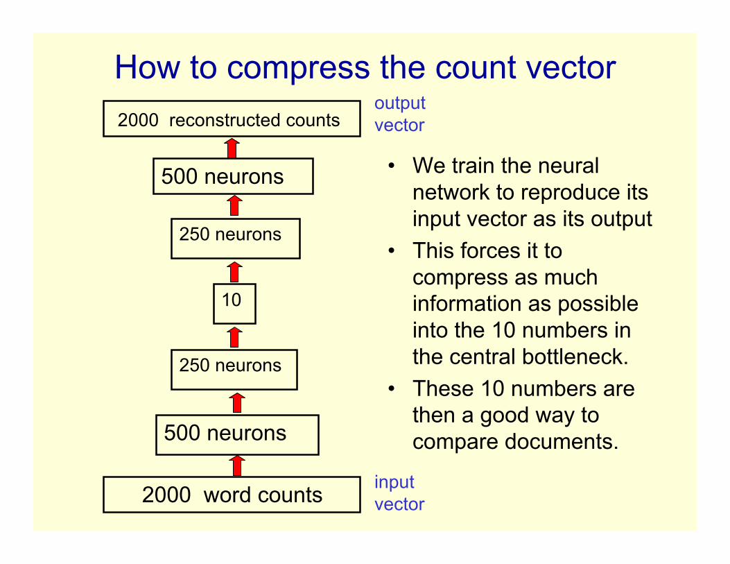
How to compress the count vector

• We train the neuralnetwork to reproduce itsinput vector as its output

• This forces it tocompress as muchinformation as possibleinto the 10 numbers inthe central bottleneck.

• These 10 numbers arethen a good way tocompare documents.

2000 reconstructed counts

500 neurons

2000 word counts

500 neurons

250 neurons

250 neurons

10

inputvector

outputvector

Performance of the autoencoder atdocument retrieval

• Train on bags of 2000 words for 400,000 training casesof business documents.– First train a stack of RBM’s. Then fine-tune with

backprop.• Test on a separate 400,000 documents.

– Pick one test document as a query. Rank order all theother test documents by using the cosine of the anglebetween codes.

– Repeat this using each of the 400,000 test documentsas the query (requires 0.16 trillion comparisons).

• Plot the number of retrieved documents against theproportion that are in the same hand-labeled class as thequery document.

Proportion of retrieved documents in same class as query

Number of documents retrieved

First compress all documents to 2 numbers using a type of PCAThen use different colors for different document categories

First compress all documents to 2 numbers.Then use different colors for different document categories

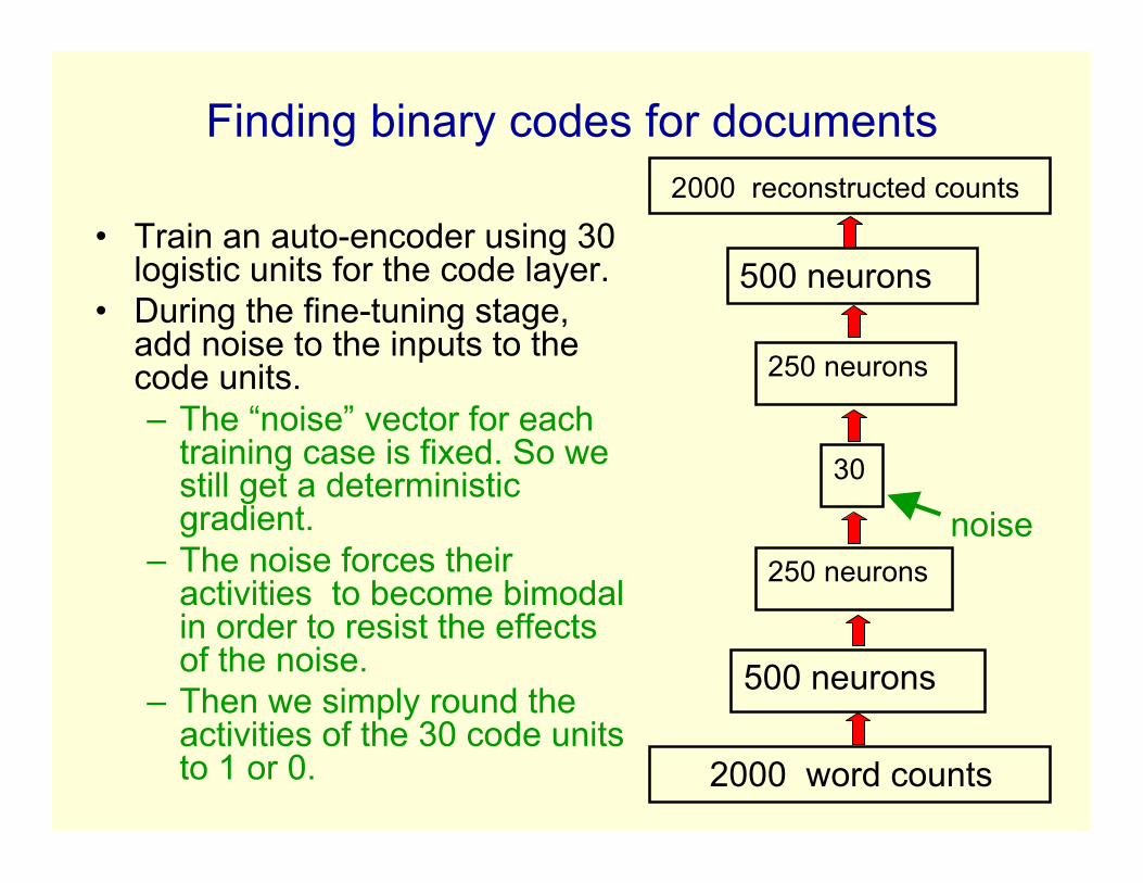
Finding binary codes for documents

• Train an auto-encoder using 30logistic units for the code layer.

• During the fine-tuning stage,add noise to the inputs to thecode units.– The “noise” vector for each

training case is fixed. So westill get a deterministicgradient.

– The noise forces theiractivities to become bimodalin order to resist the effectsof the noise.

– Then we simply round theactivities of the 30 code unitsto 1 or 0.

2000 reconstructed counts

500 neurons

2000 word counts

500 neurons

250 neurons

250 neurons

30

noise

Semantic hashing: Using a deep autoencoder as ahash-function for finding approximate matches

(Salakhutdinov & Hinton, 2007)

hashfunction

“supermarket search”

How good is a shortlist found this way?

• We have only implemented it for a milliondocuments with 20-bit codes --- but what couldpossibly go wrong?– A 20-D hypercube allows us to capture enough

of the similarity structure of our document set.• The shortlist found using binary codes actually

improves the precision-recall curves of TF-IDF.– Locality sensitive hashing (the fastest other

method) is 50 times slower and has worseprecision-recall curves.

Time series models

• Inference is difficult in directed models of timeseries if we use non-linear distributedrepresentations in the hidden units.– It is hard to fit Dynamic Bayes Nets to high-

dimensional sequences (e.g motion capturedata).

• So people tend to avoid distributedrepresentations and use much weaker methods(e.g. HMM’s).

Time series models

• If we really need distributed representations (which wenearly always do), we can make inference much simplerby using three tricks:– Use an RBM for the interactions between hidden and

visible variables. This ensures that the main source ofinformation wants the posterior to be factorial.

– Model short-range temporal information by allowingseveral previous frames to provide input to the hiddenunits and to the visible units.

• This leads to a temporal module that can be stacked– So we can use greedy learning to learn deep models

of temporal structure.

The conditional RBM model(Sutskever & Hinton 2007)

• Given the data and the previous hiddenstate, the hidden units at time t areconditionally independent.– So online inference is very easy

• Learning can be done by usingcontrastive divergence.– Reconstruct the data at time t from

the inferred states of the hidden unitsand the earlier states of the visibles.

– The temporal connections can belearned as if they were additionalbiases

t-2 t-1 t

t

)( reconjdatajiij sssw ><!><="

i

j

Why the autoregressive connections do not causeproblems

• The autoregressive connections do not mess upcontrastive divergence learning because:– We know the initial state of the visible units, so we

know the initial effect of the autoregressiveconnections.

– It is not necessary for the reconstructions to be atequilibrium with the hidden units.

– The important thing for contrastive divergence is toensure the hiddens are in equilibrium with the visibleswhenever statistics are measured.

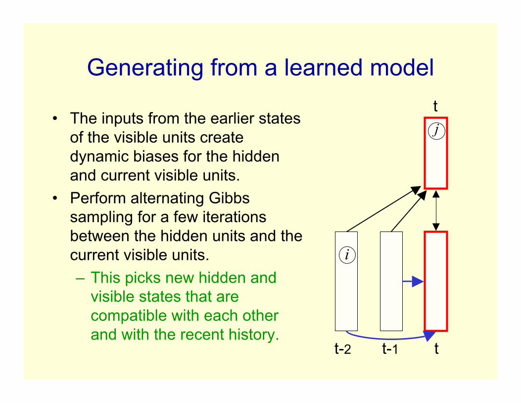
Generating from a learned model

• The inputs from the earlier statesof the visible units createdynamic biases for the hiddenand current visible units.

• Perform alternating Gibbssampling for a few iterationsbetween the hidden units and thecurrent visible units.– This picks new hidden and

visible states that arecompatible with each otherand with the recent history.

t-2 t-1 t

t

i

j

Stacking temporal RBM’s• Treat the hidden activities of the first level

TRBM as the data for the second-levelTRBM.– So when we learn the second level, we

get connections across time in the firsthidden layer.

• After greedy learning, we can generate fromthe composite model– First, generate from the top-level model

by using alternating Gibbs samplingbetween the current hiddens andvisibles of the top-level model, using thedynamic biases created by the previoustop-level visibles.

– Then do a single top-down pass throughthe lower layers, but using theautoregressive inputs coming fromearlier states of each layer.

An application to modelingmotion capture data

(Taylor, Roweis & Hinton, 2007)

• Human motion can be captured by placingreflective markers on the joints and then usinglots of infrared cameras to track the 3-Dpositions of the markers.

• Given a skeletal model, the 3-D positions of themarkers can be converted into the joint anglesplus 6 parameters that describe the 3-D positionand the roll, pitch and yaw of the pelvis.– We only represent changes in yaw because physics

doesn’t care about its value and we want to avoidcircular variables.

Modeling multiple types of motion

• We can easily learn to model walking andrunning in a single model.– This means we can share a lot of knowledge.– It should also make it much easier to learn

nice transitions between walking and running.• In a switching mixture of dynamical systems its

hard to get the latent variables to join up nicelywhen we switch from one system to another.

• Because we can do online inference (slightlyincorrectly), we can fill in missing markers in realtime.

Show Graham Taylor’s movies

available at www.cs.toronto/~hinton

Generating the parts of an object

• One way to maintain theconstraints between the parts isto generate each part veryaccurately– But this would require a lot of

communication bandwidth.• Sloppy top-down specification of

the parts is less demanding– but it messes up relationships

between features– so use redundant features

and use lateral interactions toclean up the mess.

• Each transformed feature helpsto locate the others– This allows a noisy channel

sloppy top-downactivation of parts

clean-up usingknown interactions

pose parameters

features withtop-downsupport

“square” +

Its like soldiers ona parade ground

Semi-restricted Boltzmann Machines• We restrict the connectivity to make

learning easier.• Contrastive divergence learning requires

the hidden units to be in conditionalequilibrium with the visibles.– But it does not require the visible units

to be in conditional equilibrium withthe hiddens.

– All we require is that the visible unitsare closer to equilibrium in thereconstructions than in the data.

• So we can allow connections betweenthe visibles.

hidden

i

j

visible

Learning a semi-restricted Boltzmann Machine

0>< jihv

1>< jihv

i

j

i

j

t = 0 t = 1

)( 10><!><=" jijiij hvhvw #

1. Start with atraining vector on thevisible units.

2. Update all of thehidden units inparallel

3. Repeatedly updateall of the visible unitsin parallel usingmean-field updates(with the hiddensfixed) to get a“reconstruction”.

4. Update all of thehidden units again.

reconstructiondata

)( 10><!><=" kikiik vvvvl #

k i ik k k

update for alateral weight

Learning in Semi-restricted BoltzmannMachines

• Method 1: To form a reconstruction, cyclethrough the visible units updating each in turnusing the top-down input from the hiddens plusthe lateral input from the other visibles.

• Method 2: Use “mean field” visible units thathave real values. Update them all in parallel.– Use damping to prevent oscillations

)()(11i

ti

ti xpp !"" #+=+

total input to idamping

Results on modeling natural image patchesusing a stack of RBM’s (Osindero and Hinton)

• Stack of RBM’s learned one at a time.• 400 Gaussian visible units that see

whitened image patches– Derived from 100,000 Van Hateren

image patches, each 20x20• The hidden units are all binary.

– The lateral connections arelearned when they are the visibleunits of their RBM.

• Reconstruction involves letting thevisible units of each RBM settle usingmean-field dynamics.– The already decided states in the

level above determine the effectivebiases during mean-field settling.

Directed Connections

Directed Connections

Undirected Connections

400Gaussianunits

HiddenMRF with2000 units

HiddenMRF with500 units

1000 top-level units.No MRF.

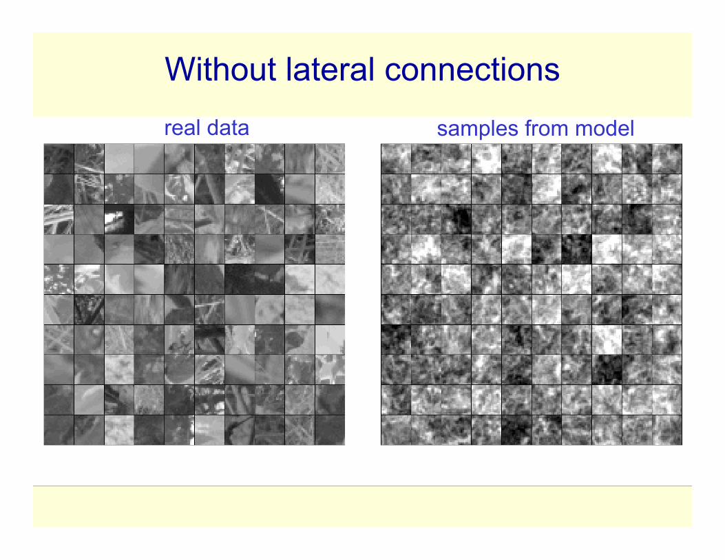
Without lateral connectionsreal data samples from model

With lateral connectionsreal data samples from model

A funny way to use an MRF

• The lateral connections form an MRF.• The MRF is used during learning and generation.• The MRF is not used for inference.

– This is a novel idea so vision researchers don’t like it.• The MRF enforces constraints. During inference,

constraints do not need to be enforced because the dataobeys them.– The constraints only need to be enforced during

generation.• Unobserved hidden units cannot enforce constraints.

– This requires lateral connections or observeddescendants.

Why do we whiten data?

• Images typically have strong pair-wise correlations.• Learning higher order statistics is difficult when there are

strong pair-wise correlations.– Small changes in parameter values that improve the

modeling of higher order statistics may be rejectedbecause they form a slightly worse model of the muchstronger pair-wise statistics.

• So we often remove the second-order statistics beforetrying to learn the higher-order statistics.

Whitening the learning signal insteadof the data

• Contrastive divergence learning can remove the effectsof the second-order statistics on the learning withoutactually changing the data.– The lateral connections model the second order

statistics– If a pixel can be reconstructed correctly using second

order statistics, its will be the same in thereconstruction as in the data.

– The hidden units can then focus on modeling high-order structure that cannot be predicted by the lateralconnections.

• For example, a pixel close to an edge, where interpolationfrom nearby pixels causes incorrect smoothing.

Towards a more powerful, multi-linearstackable learning module

• So far, the states of the units in one layer have only beenused to determine the effective biases of the units in thelayer below.

• It would be much more powerful to modulate the pair-wiseinteractions in the layer below. (A good way to design ahierarchical system is to allow each level to determine theobjective function of the level below.)– For example, a vertical edge represents a breakdown in

the usual correlational structure of the pixels: Horizontalinterpolation does not work, so it needs to be turned off,but interpolation parallel to the edge is OK.

• To modulate pair-wise interactions we need higher-orderBoltzmann machines.

Higher order Boltzmann machines(Sejnowski, ~1986)

• The usual energy function is quadratic in the states:

• But we could use higher order interactions:

ijj

ji

i wsstermsbiasE !<

"=

ijkkj

kji

i wssstermsbiasE !<<

"=

• Unit k acts as a switch. When unit k is on, it switchesin the pairwise interaction between unit i and unit j.– Units i and j can also be viewed as switches that

control the pairwise interactions between j and kor between i and k.

A picture of a conditional, higher-order Boltzmann machine

(Hinton & Lang,1985)

retina-basedfeatures

object-basedfeaturesviewing

transform

• We can view it as aBoltzmann machine inwhich the inputs createinteractions between theother variables.– This type of model is

now called a conditionalrandom field.

– It is hard to learn withtwo hidden groups.

Using conditional higher-order Boltzmannmachines to model image transformations

(Memisevic and Hinton, 2007)

• A transformation unit specifies which pixel goesto which other pixel.

• Conversely, each pair of similar intensity pixels,one in each image, votes for all the compatibletransformation units.

image(t) image(t+1)

image transformation

Readings on deep belief nets

A reading list (that is still being updated) can befound at

www.cs.toronto.edu/~hinton/csc2515/deeprefs.html