a dynamic model of health, addiction, education, and wealth · a dynamic model of health,...
TRANSCRIPT

A Dynamic Model of Health, Addiction, Education, andWealth∗
Rong Hai and James J. Heckman
2016/09/02
Abstract
This paper formulates and estimates a dynamic model of education, health, andwealth in which agents consume unhealthy addictive goods. They differ in their endow-ments of cognitive and noncognitive skills and face endogenously-determined borrowingconstraints. The consumption of unhealthy addictive goods, low levels of cognitive andnoncognitive skills, and limited access to the borrowing market explain the constella-tion of poor health, low levels of education, and wealth. The model is estimated usingdata from National Longitudinal Survey of Youth 97, using a two-step estimation pro-cedure that combines factor analysis and the simulated method of moments. We testthe rational addiction model by comparing its fit to data. We evaluate the impacts of arevenue-neutral excise tax on unhealthy goods and improvements in early endowmentson health, education, and wealth over the life cycle.
JEL codes: I1, I2, J2Keywords: Health Capital, Education, Wealth, Human Capital, Rational Addiction,
Credit Constraints, Unhealthy Behavior
∗We thank Siddhartha Biswas for excellent research assistance. We thank Victor Aguirregabiria, JosephAltonji, Gadi Barlevy, Stephane Bonhomme, John Cawley, Indraneel Chakraborty, Flavio Cunha, Mari-acristina De Nardi, David Frisvold, Martin Gervais, Donna Gilleskie, Limor Golan, Luojia Hu, ArieKapteyn, Donald Kenkel, John Kennan, Arnaud Maurel, Costas Meghir, Ronni Pavan, Peter Savelyev,Steven Stern, Anne Villamil, Alessandra Voena, seminar participants at Cornell University, Universityof Chicago, University of Iowa, University of Miami, University of Rochester, Federal Reserve Bank ofChicago, Cowles Summer Conference on Structure Empirical Microeconomic Models, 11th World Congressof Econometric Society, 2014 Annual Health Econometrics Workshop, Fifth Biennial Meeting of the Amer-ican Society of Health Economists, Launch Event of the Center for the Economics of Human Develop-ment for helpful comments and suggestions. Rong Hai: University of Miami, [email protected]. JamesJ. Heckman: University of Chicago, [email protected]. A web appendix for this paper can be found athttps://heckman.uchicago.edu/dyn_model_addiction_health.
1
A Dynamic Model of Health, Addiction, Education, and Wealth
1 Introduction
There is a well-established positive relationship between health and levels of education and
wealth.1 To understand this relationship, we construct an empirical model of consumption of
unhealthy addictive goods, education, credit constraints, and the role of early endowments
and parental background.
Our model has four key features. The first feature is that human capital, wealth, and
health capital are endogenous. We characterize dynamic relationships among these variables.
The second feature is the analysis of consumption of addictive unhealthy goods. In the U.S.
and many other developed countries, substantial components of cross-sectional differences
in health outcomes are attributed to differences in unhealthy addictive behavior (such as
smoking and heavy drinking) (McGinnis, Williams-Russo, and Knickman, 2002; Smith, 2007;
Chen, Smith, Harbord, and Lewis, 2008; Sloan, Ostermann, Conover, Taylor, and Picone,
2004; Centers for Disease Control and Prevention, 2010). The third key feature is our analysis
of endogenous credit constraints and parental influence. In the presence of credit constraints,
individuals with low current wealth under-invest in their health and human capital. A fourth
key feature is that we examine the roles of cognitive and noncognitive skills in explaining
this relationship.
In one version of our model, individuals are allowed to make rational far-sighted decisions
on schooling, unhealthy behavior, and savings for each age in order to maximize expected
lifetime utility. We test a myopic model against a rational addiction model and find support
for the rational model. Because of uncertainty there is ex post regret. Education affects
health dynamics by directly enhancing the production of health and by affecting individual
choices of health production inputs.
Health affects individual choices of education and wealth in four ways. First, health affects
wages. Second, health affects psychic costs associated with schooling. Third, health shapes
subjective discount rates, which effectively alter decision horizons, and thus affect investment
1See Deaton (2015), Grossman (2008), and Goldman and Smith (2011).
1
A Dynamic Model of Health, Addiction, Education, and Wealth
decisions about human capital and wealth. Fourth, current health directly impacts the stock
of future health. Through the budget constraint and borrowing constraint, wealth impacts
education and health.
Our model has several sources of heterogeneity among agents: (1) Individuals differ in
their initial endowments of cognitive and noncognitive abilities and health. These initial
endowments not only directly impact individuals’ later life outcomes such as earnings and
health, but also affect individuals’ investment behavior in schooling and unhealthy behavior.
(2) Parents differ in education and wealth. Both parental education and wealth affect the
transfers the individual receives in college. In addition, parental education shifts individual
preferences towards schooling. (3) We generate heterogeneity in health, education, wealth,
and patterns of addictive consumption across individuals over time as a result of rational
investment behavior in the presence of financial market imperfections. Individuals face an
endogenous borrowing limit which explicitly depends on their lifecycle earnings process. All
three sources of heterogeneity are quantitative important sources of the cross-sectional and
life cycle inequality for health, education, and wealth.
The model is estimated in two steps using data from the National Longitudinal Survey of
Youth 1997 (NLSY97). The first step estimates a measurement system to identify unobserved
cognitive and noncognitive abilities and health. In the second step, we structurally estimate
the behavioral model using the simulated method of moments (SMM).
We find evidence of substantial sorting into adult education based on youths’ initial
health and early cognitive and noncognitive endowments. Our estimates suggests that the
direct benefits of health on schooling is sizable. We compare our forward-looking model to a
counterfactual model where individuals make myopic decisions on their unhealthy goods con-
sumption. The myopic model over-predicts the probability of engaging unhealthy behavior,
especially at the beginning and at the end of lifecycle.
We also use our model to conduct two counterfactual policy experiments. First, we
introduce a revenue-neutral excise tax on unhealthy goods. We find that such policy leads
2

A Dynamic Model of Health, Addiction, Education, and Wealth
to higher levels of average health, schooling, earnings, and wealth, and reduces inequality
in health, schooling, earnings, and wealth. However, the excise tax reduces consumption
level on normal goods and increases consumption inequality. Second, we introduce an early
intervention program that increases adolescent cognitive ability and noncognitive ability
among the most disadvantaged population. This policy not only increases average levels of
health, schooling, earnings and consumption, but also reduces inequality measured in these
dimensions as well.
Our paper contributes to three strands of literature. First, our model extends the litera-
ture on health capital proposed by Grossman (1972). He models health as a durable capital
stock and shows that the demand for health increases with education if more educated people
are more efficient producers of health.2 Since then, a substantial body of research investi-
gates the relationship between health and other socioeconomic factors including education,
income, wealth, and family background.3 An education gradient is found for both health
behaviors and health status.4 Part of the relationship between education and health behav-
iors is explained by differences in health knowledge (Kenkel, 1991). Conti, Heckman, and
Urzua (2010) show that family background characteristics, and cognitive, noncognitive, and
health endowments developed at an earlier age are important determinants of labor market
and health disparities in later years. Heckman, Humphries, and Veramendi (2016b) show
that education at all levels causally produces gains in health and that early cognitive and
socio-emotional ability have important effects on health outcomes and schooling choices.
Savelyev and Tan (2014) find strong effects of education and personality skills on health and
health-related outcomes. De Nardi, French and Jones (2009; 2010) investigate the effect of
health on the saving behavior of the elderly.
Second, our paper contributes to the rational addiction literature following the analysis
of Becker and Murphy (1988). A substantial body of empirical research tests the empir-
2Galama (2011) and Galama and van Kippersluis (2010) provide theoretical frameworks through whicheducation and wealth may impact the disparity in health.
3See Deaton (2003), Currie (2009), Cutler and Lleras-Muney (2010), and Heckman, Humphries, andVeramendi (2016b).
4Cutler and Lleras-Muney (2006).
3
A Dynamic Model of Health, Addiction, Education, and Wealth
ical implications of the rational addiction model. Becker, Grossman, and Murphy (1991,
1994) find that the short-run price elasticity of cigarette consumption is negative and that
long-run responses exceed short-run responses. Chaloupka (1991) and Gruber and Koszegi
(2001) provide evidence that cigarette smoking is an addictive behavior and smokers are
forward-looking in their smoking decisions. Adda and Cornaglia (2006) apply the ratio-
nal addiction model to study smoking intensity and show that smokers compensate for tax
hikes by extracting more nicotine per cigarette. Grossman, Chaloupka, and Sirtalan (1998)
estimate the addictive properties of alcohol. The model has also been applied to caffeine
(Olekalns and Bardsley, 1996) and cocaine (Grossman and Chaloupka, 1998). Sundmacher
(2012) finds that health shocks have a significant positive impact on the probability that
smokers quit during the year in which they experience health shocks, providing evidence
that smokers are aware of the risks associated with tobacco consumption and are willing to
quit for health-related reasons.
Our paper also contributes to the literature on credit constraints and schooling. The
evidence on it is mixed (Heckman and Mosso, 2014). Using the National Longitudinal Survey
of Youth 1979 (NLSY79) data, Keane and Wolpin (2001) show that although borrowing
constraints exist, they have no quantitative impact on youth schooling decisions. Cameron
and Taber (2004) reject the hypothesis that there are binding credit constraints in NLSY79
data. Using NLSY79 and NLSY79 Children (CNLSY79), Carneiro and Heckman (2002) find
that the role of family income in determining college enrollment decisions is negligible once
ability is controlled. More recent studies suggest that borrowing constraints in recent years
may play a bigger role in college enrollment for the National Longitudinal Survey of Youth
1997 (NLSY97) cohorts.5 Navarro (2011a) reports that there are sizable effects of relaxing
borrowing constraints on schooling decisions whereas the effects of reducing tuition are very
small. Hai and Heckman (2016) find substantial quantitative evidence of credit constraints
on educational choices.
5See Belley and Lochner (2007), Bailey and Dynarski (2011), and Lochner and Monge-Naranjo (2012a).
4
A Dynamic Model of Health, Addiction, Education, and Wealth
2 Model
This section presents, in order, our model, our method of numerically solving the model, our
initial conditions, and our measurement system.
2.1 Model Specification
2.1.1 Choice Set
At each age t = t0, . . . T , an individual makes decisions about: (i) consumption (ct) and
savings (st+1), (ii) whether to engage in unhealthy behavior (dq,t ∈ 0, 1), (iii) whether to
go to school (de,t ∈ 0, 1), and (iv) whether to work part-time while in school (dp,t ∈ 0, 1).
2.1.2 State Variables
At each age t, an individual is characterized by a vector of state variables that shape pref-
erences, production technology, and outcomes:
Ωt := (t,θ, et, st, ht, qt, de,t−1, ep, sp) (1)
where θ is a vector that summarizes individual components of unobserved cognitive ability
and noncognitive ability, et is years of schooling at t, st is net worth determined at the end
of period t − 1, ht is the individual’s age-t health stock, qt is the stock of addiction capital
accumulated from past unhealthy behavior (“habit”), de,t−1 is the schooling status in period
t, ep is parental educational level, and sp is parental net worth. The information set, that
includes all of the state variables and realized idiosyncratic shocks at age t (εt), can be
written as Ωt := Ωt, εt.
5
A Dynamic Model of Health, Addiction, Education, and Wealth
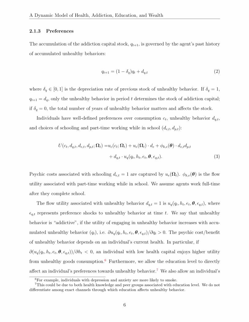
2.1.3 Preferences
The accumulation of the addiction capital stock, qt+1, is governed by the agent’s past history
of accumulated unhealthy behaviors:
qt+1 = (1− δq)qt + dq,t (2)
where δq ∈ [0, 1] is the depreciation rate of previous stock of unhealthy behavior. If δq = 1,
qt+1 = dq, only the unhealthy behavior in period t determines the stock of addiction capital;
if δq = 0, the total number of years of unhealthy behavior matters and affects the stock.
Individuals have well-defined preferences over consumption ct, unhealthy behavior dq,t,
and choices of schooling and part-time working while in school (de,t, dp,t):
U(ct, dq,t, de,t, dp,t; Ωt) =uc(ct; Ωt) + ue(Ωt) · de + φk,e(θ) · de,tdp,t
+ dq,t · uq(qt, ht, et,θ, εq,t). (3)
Psychic costs associated with schooling de,t = 1 are captured by ue(Ωt). φk,e(θ) is the flow
utility associated with part-time working while in school. We assume agents work full-time
after they complete school.
The flow utility associated with unhealthy behavior dq,t = 1 is uq(qt, ht, et,θ, εq,t), where
εq,t represents preference shocks to unhealthy behavior at time t. We say that unhealthy
behavior is “addictive”, if the utility of engaging in unhealthy behavior increases with accu-
mulated unhealthy behavior (qt), i.e. ∂uq(qt, ht, et,θ, εq,t)/∂qt > 0. The psychic cost/benefit
of unhealthy behavior depends on an individual’s current health. In particular, if
∂(uq(qt, ht, et,θ, εq,t))/∂ht < 0, an individual with low health capital enjoys higher utility
from unhealthy goods consumption.6 Furthermore, we allow the education level to directly
affect an individual’s preferences towards unhealthy behavior.7 We also allow an individual’s
6For example, individuals with depression and anxiety are more likely to smoke.7This could be due to both health knowledge and peer groups associated with education level. We do not
differentiate among exact channels through which education affects unhealthy behavior.
6

A Dynamic Model of Health, Addiction, Education, and Wealth
preferences for unhealthy behavior to be directly affected by cognitive ability and noncog-
nitive ability. By explicitly allowing for both time-dependent preferences in the stock of
addictive capital and forward-looking maximizing behavior, our model can generate ratio-
nal addiction as one possible outcome. However, we do not force rational addiction on our
estimated model.
Agents discount future returns using a subjective discount factor exp(−ρ(θ, ht)), where
ρ(θ, ht) > 0 is the subjective discount rate. The dependence of the discount rate on both
cognitive ability and noncognitive ability captures findings in the recent literature (Dohmen,
Falk, Huffman, Sunde, Schupp, and Wagner, 2011). Allowing the discount rate to depend on
health, we implicitly account for mortality.8 Healthy individuals have a longer life expectancy
and a longer decision horizon, thus they effectively have a relatively lower discount rate.
2.1.4 Health Capital Production
Health capital at age t+ 1, ht+1 > 0, is produced according to the following relationship:9
ht+1 = H(ht, dq,t, ct, et,θ, t, εh,t) (4)
where εh,t is an idiosyncratic shock at age t that affects the health capital stock at age
t + 1. Equation (4) allows health capital at age t + 1 to depend on health capital at age
t. Health capital can also be affected by individual decisions regarding unhealthy behavior
and consumption.10 Lastly, education and cognitive and noncognitive skills can also directly
impact health by affecting the allocative efficiency in health production (see Grossman,
1972).
8We do not explicitly model mortality because individuals are relatively young in our sample (see Section3) and we do not observe the event of death.
9The health production function abstracts from health insurance, this is because education is a goodindicator of health insurance coverage in the current employment-based health insurance system, and alsobecause previous research finds the effect of health insurance on health is small (if any).
10We do not explicitly distinguish the role of medical care from other consumption expenditure, because wedo not observe medical care expenditure in our data. Furthermore, individuals in our sample are relativelyyoung, medical expenditure is less important.
7

A Dynamic Model of Health, Addiction, Education, and Wealth
Engaging in unhealthy behavior today reduces next period health capital if H(ht, dq,t =
1, ct, et,θ, t, εh,t) < H(ht, dq,t = 0, ct, et,θ, t, εh,t). Everything else equal, an individual with
higher earnings and/or assets can boost next period equal health level by changing consump-
tion levels.
2.1.5 Earnings Process Based on an Individual’s Human Capital
Earnings at age t after leaving school, depend on health, education, experience, and cognitive
and noncognitive abilities:
yt = Fψ(ht, et, kt,θ, εy,t). (5)
where kt = max0, t − et + 12 is the individual’s work experience and εy,t ∈ [εy, εy] is a
time-idependent idiosyncratic earnings shock at age t. The earnings for an individual who
works part-time while in school dp,t = 1 is given by βw,p · 12Fψ(ht, et, kt,θ, εy,t). Education
level at age t+ 1, measured by years of schooling, is:
et+1 = et + de,t. (6)
2.1.6 Financial Markets and Endogenous Credit Constraints
We explicitly model the credit constraints facing agents. While in school, agents can borrow
from the private market or from guaranteed loan programs. We consider loans from parents
and parental transfers in the next subsection.
To finance their education and consumption, individuals can borrow at riskless exogenous
interest rate rb. An individual can also lend to the market at riskless rate of return rl.11 To
capture an important feature of imperfect capital markets, we allow the lending rate to be
smaller than the borrowing rate, i.e., rl < rb.12
Borrowing is limited by repayment ability. The smallest amount of net worth st+1 that
11We abstract away from portfolio choices.12We only keep track of an agent’s net worth so there is no need to separately keep track of an agent’s
physical capital debts and assets. Furthermore, when rl < rb, an individual never finds it optimal to be botha borrower and a lender.
8
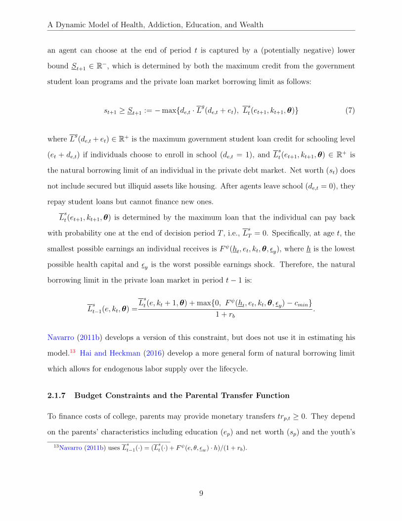
A Dynamic Model of Health, Addiction, Education, and Wealth
an agent can choose at the end of period t is captured by a (potentially negative) lower
bound St+1 ∈ R−, which is determined by both the maximum credit from the government
student loan programs and the private loan market borrowing limit as follows:
st+1 ≥ St+1 := −maxde,t · Lg(de,t + et), L
s
t(et+1, kt+1,θ) (7)
where Lg(de,t + et) ∈ R+ is the maximum government student loan credit for schooling level
(et + de,t) if individuals choose to enroll in school (de,t = 1), and Ls
t(et+1, kt+1,θ) ∈ R+ is
the natural borrowing limit of an individual in the private debt market. Net worth (st) does
not include secured but illiquid assets like housing. After agents leave school (de,t = 0), they
repay student loans but cannot finance new ones.
Ls
t(et+1, kt+1,θ) is determined by the maximum loan that the individual can pay back
with probability one at the end of decision period T , i.e., Ls
T = 0. Specifically, at age t, the
smallest possible earnings an individual receives is Fψ(ht, et, kt,θ, εy), where h is the lowest
possible health capital and εy is the worst possible earnings shock. Therefore, the natural
borrowing limit in the private loan market in period t− 1 is:
Ls
t−1(e, kt,θ) =Ls
t(e, kt + 1,θ) + max0, Fψ(ht, et, kt,θ, εy)− cmin1 + rb
.
Navarro (2011b) develops a version of this constraint, but does not use it in estimating his
model.13 Hai and Heckman (2016) develop a more general form of natural borrowing limit
which allows for endogenous labor supply over the lifecycle.
2.1.7 Budget Constraints and the Parental Transfer Function
To finance costs of college, parents may provide monetary transfers trp,t ≥ 0. They depend
on the parents’ characteristics including education (ep) and net worth (sp) and the youth’s
13Navarro (2011b) uses Ls
t−1(·) = (Ls
t (·) + Fψ(e, θ, εw) · h)/(1 + rb).
9

A Dynamic Model of Health, Addiction, Education, and Wealth
own schooling decisions de,t as well as the youth’s own education level and age:14
trp,t = trp(ep, sp, de,t, et, t). (8)
Examples of parental monetary transfers include college financial gifts if the youth chooses
to attend college. The parental transfer rule is taken as given. This captures paternalism
and tied transfers on the part of the parents, which is consistent with the findings of pre-
vious research (see, e.g., Keane and Wolpin, 2001 and Johnson, 2013). See the evidence
summarized in Heckman and Mosso (2014).
Defining r(st) := rl1(st > 0) + rb1(st < 0), the budget constraint for an individual who
chooses to attend college (i.e., de,t · 1(et + de,t > 13) = 1) is:
ct + pqdq,t + (tc(et + de,t)− gr(et + de,t, sp, θ)) + st+1 = (1 + r(st)) · st + βw,pyt2· dp,t + trp,t
(9)
ct ≥ rc(et + de,t) (10)
where pq is the monetary cost of unhealthy behavior, tc(et+de,t) is the cost of college tuition
and fees, gr(et+de,t, sp) is the amount of grants and scholarships which depend on schooling
level and parental wealth, rc(et + de,t) denotes the cost of college room and board, and
βw,pyt/2 is the earnings from part-time working while in school.15
The budget constraint for a person not currently enrolled in college (i.e., de,t ·1(et+de,t >
13) = 0) is:
ct + pqdq,t + st+1 = (1 + r(st)) · st + yt + trp,t + trc,t + trg,t (11)
ct ≥ cmin (12)
where trc,t ≥ 0 is the direct consumption subsidy from the parents to their dependent child
14This is an extension of the parental transfer function in Keane and Wolpin (2001).15College part-time work is assumed to be half-time.
10
A Dynamic Model of Health, Addiction, Education, and Wealth
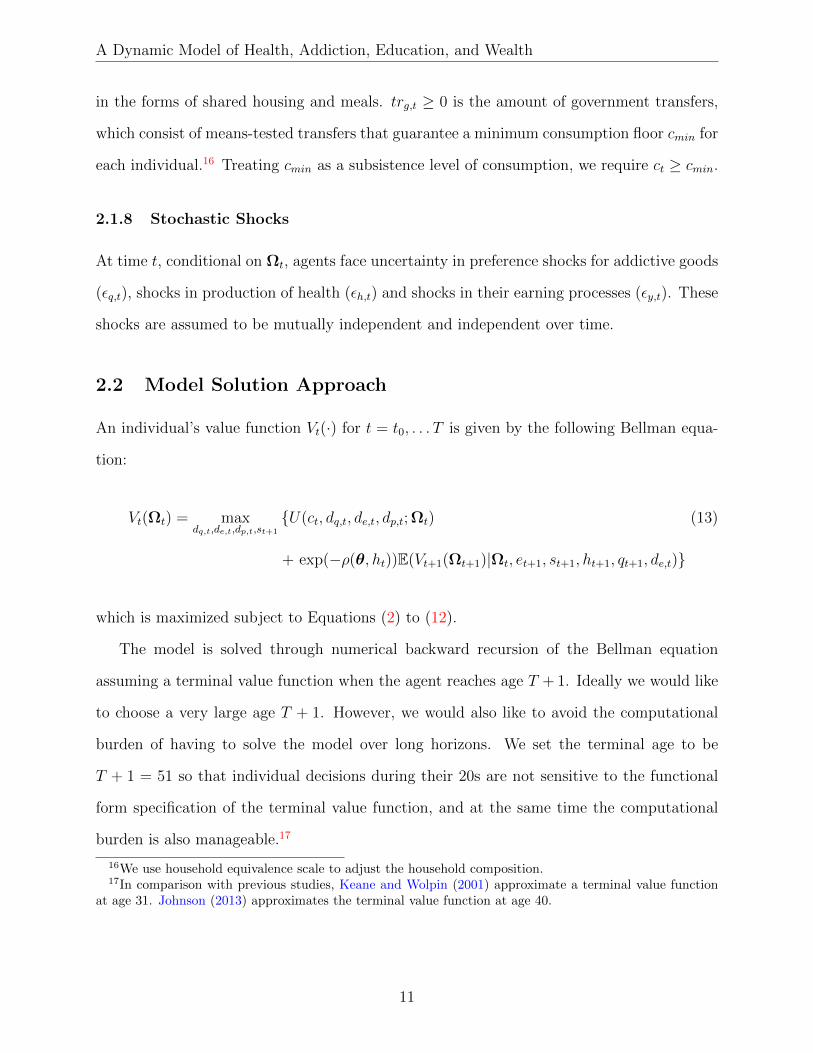
in the forms of shared housing and meals. trg,t ≥ 0 is the amount of government transfers,
which consist of means-tested transfers that guarantee a minimum consumption floor cmin for
each individual.16 Treating cmin as a subsistence level of consumption, we require ct ≥ cmin.
2.1.8 Stochastic Shocks
At time t, conditional on Ωt, agents face uncertainty in preference shocks for addictive goods
(εq,t), shocks in production of health (εh,t) and shocks in their earning processes (εy,t). These
shocks are assumed to be mutually independent and independent over time.
2.2 Model Solution Approach
An individual’s value function Vt(·) for t = t0, . . . T is given by the following Bellman equa-
tion:
Vt(Ωt) = maxdq,t,de,t,dp,t,st+1
U(ct, dq,t, de,t, dp,t; Ωt) (13)
+ exp(−ρ(θ, ht))E(Vt+1(Ωt+1)|Ωt, et+1, st+1, ht+1, qt+1, de,t)
which is maximized subject to Equations (2) to (12).
The model is solved through numerical backward recursion of the Bellman equation
assuming a terminal value function when the agent reaches age T + 1. Ideally we would like
to choose a very large age T + 1. However, we would also like to avoid the computational
burden of having to solve the model over long horizons. We set the terminal age to be
T + 1 = 51 so that individual decisions during their 20s are not sensitive to the functional
form specification of the terminal value function, and at the same time the computational
burden is also manageable.17
16We use household equivalence scale to adjust the household composition.17In comparison with previous studies, Keane and Wolpin (2001) approximate a terminal value function
at age 31. Johnson (2013) approximates the terminal value function at age 40.
11
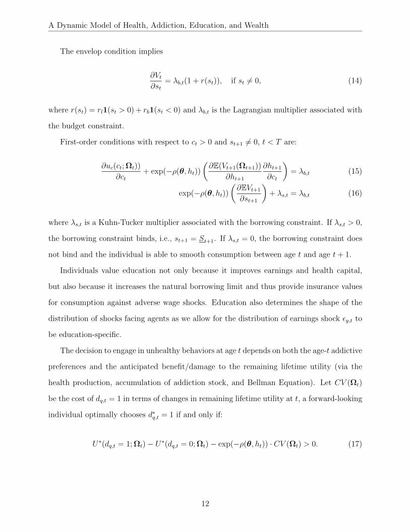
A Dynamic Model of Health, Addiction, Education, and Wealth
The envelop condition implies
∂Vt∂st
= λb,t(1 + r(st)), if st 6= 0, (14)
where r(st) = rl1(st > 0) + rb1(st < 0) and λb,t is the Lagrangian multiplier associated with
the budget constraint.
First-order conditions with respect to ct > 0 and st+1 6= 0, t < T are:
∂uc(ct; Ωt))
∂ct+ exp(−ρ(θ, ht))
(∂E(Vt+1(Ωt+1))
∂ht+1
∂ht+1
∂ct
)= λb,t (15)
exp(−ρ(θ, ht))
(∂EVt+1
∂st+1
)+ λs,t = λb,t (16)
where λs,t is a Kuhn-Tucker multiplier associated with the borrowing constraint. If λs,t > 0,
the borrowing constraint binds, i.e., st+1 = St+1. If λs,t = 0, the borrowing constraint does
not bind and the individual is able to smooth consumption between age t and age t+ 1.
Individuals value education not only because it improves earnings and health capital,
but also because it increases the natural borrowing limit and thus provide insurance values
for consumption against adverse wage shocks. Education also determines the shape of the
distribution of shocks facing agents as we allow for the distribution of earnings shock εy,t to
be education-specific.
The decision to engage in unhealthy behaviors at age t depends on both the age-t addictive
preferences and the anticipated benefit/damage to the remaining lifetime utility (via the
health production, accumulation of addiction stock, and Bellman Equation). Let CV (Ωt)
be the cost of dq,t = 1 in terms of changes in remaining lifetime utility at t, a forward-looking
individual optimally chooses d∗q,t = 1 if and only if:
U∗(dq,t = 1; Ωt)− U∗(dq,t = 0; Ωt)− exp(−ρ(θ, ht)) · CV (Ωt) > 0. (17)
12
A Dynamic Model of Health, Addiction, Education, and Wealth
where U∗(dq,t; Ωt) is the flow utility associated with dq,t.18 The net benefit of unhealthy be-
havior in terms of flow utility, U∗(dq,t = 1; Ωt)− U∗(dq,t = 0; Ωt), is directly affected by age-t
addiction capital (qt), health (ht), education (et), cognitive ability and noncognitive ability
(θ) via the preference function uq(qt, ht, et,θ, εq,t) associated with qt = 1. Furthermore, as
an individual’s health deteriorates, exp(−ρ(θ, ht)) becomes smaller, the effects coming from
CV (Ωt) becomes smaller.
Finally, CV (Ωt), the cost of dq,t = 1 in terms of changes in remaining life time utility,
consists of a choice of “health capital effect” and an “addictive preference effect”:
CV (Ωt) := E(Vt+1|Ωt, h
∗t+1(0), qt+1 = (1− δq)qt
)− E
(Vt+1|Ωt, h
∗t+1(1), qt+1 = (1− δq)qt + 1
)where h∗t+1(dq,t) is the age t+1 health capital associated with dq,t, and E(Vt+1|h∗t+1(dq,t), qt+1 =
(1− δq)qt + dq,t) is the lifetime utility at age t + 1 associated with dq,t.19 On the one hand,
engaging in unhealthy behavior decreases the health capital level in the next period, ceteris
paribus, and thus reduces the remaining life-time utility, because health affects both labor
market wages and psychic costs of schooling. On the other hand, engaging in unhealthy
behavior in period t increases addiction capital and thus leads to an increase in future utility
associated with dq,t+1 = 1 when unhealthy behavior is addictive (i.e., ∂uq/∂q > 0).
2.3 Initial Distribution and Our Measurement System
The model is completed by defining its initial conditions and a set of measurement equations
that relate the unobserved ability endowments and latent health level to observed measures.
Individuals start to make decisions at age 17 (t0 = 17). The deterministic components of
18More precisely, U∗(dq,t; Ωt) := U(c∗t (dq,t), dq,t, d∗e,t(dq,t), d
∗p,t(dq,t); Ωt), where c∗t (dq,t), d∗e,t(dq,t),
d∗p,t(dq,t) are the optimal choices on consumption, schooling, and working associated for a given dq,t ∈ 0, 1.19Et(Vt+1|Ωt, dq,t) := Et(Vt+1(Ωt+1)|Ωt, et+1 = et + d∗e,t(dq,t), s
∗t+1(dq,t), h
∗t+1(dq,t), qt+1 = (1 − δq)qt +
dq,t, d∗e,t(dq,t)) where d∗e,t(dq,t), s
∗t+1(dq,t), h
∗t+1(dq,t) are the optimal schooling and savings decisions associ-
ated with dq,t ∈ 0, 1.
13
A Dynamic Model of Health, Addiction, Education, and Wealth
age 17 information set, Ω17 is given by:
Ω17 ≡ (17, h17, θc, θn, e17, s17, q17, de,16, ep, sp).
The observed initial condition at age 17 from the data is as follows,20
Ωobserved
17 ≡ (17, e17, s17, q17, de,16, ep, sp).
The unobserved endowments in cognitive ability, noncognitive ability, and the logarithm
of health at age 17 are assumed to be jointly normal distributed. Furthermore, because
these early endowments are either inherited from the parents (e.g., genes) or formed as the
result of parental early investment, we allow the distribution of initial endowments to differ
by parental characteristics (i.e., parental education and wealth in our model). In particular,
the joint distribution of the unobserved cognitive ability, noncognitive ability, and health at
initial age 17 is given by the following:
θc
θn
log h17
X17 ∼ N
µc(ep, sp)
µn(ep, sp)
µh(ep, sp)
,
σ2c
σc,n σ2n
σc,h σn,h σ2h
where µj(ep, sp) = µj,e,11(ep = 12)+µj,e,21(ep > 12 & ep < 16)+µj,e,31(ep ≥ 16)+µj,s,11(sp =
2) + µj,s,21(sp = 3), for j = c, n, h.
We lack direct measurements of cognitive, noncognitive, and health endowments. Instead,
we observe a set of measurement equations for θc, θn, log h17. Specifically, we assume that at
age 17 there exist three sets of dedicated measurement equations for (θc, θn, log ht) given by
20Education, school attendance, parental education, and parental wealth (e17, de,16, ep, sp) are directlyobtained from data. We set the net worth at age 17 to be zero (s17 = 0). We set the addiction habit at age17 to be q17 = dq,16 + (1− δq)dq,15.
14
A Dynamic Model of Health, Addiction, Education, and Wealth
Equations (18), (19), and (20), respectively:
Z∗c,j = µz,c,j + αz,c,jθc + εz,c,j, j = 1, . . . , Jc (18)
Z∗n,j = µz,n,j + αz,n,jθn + εz,n,j, j = 1, . . . , Jn (19)
Z∗ht,j = µz,h,j + αz,h,j log ht + εz,ht,j, j = 1, . . . , Jh (20)
where individual control variables, including parental education and wealth, initial education
level, and lagged schooling are omitted from the measurement equations. The measurement
errors εz,c,j, εz,n,j, εz,ht,j are assumed to be independently distributed within and across blocks
of equations. The unconditional distribution of (θc, θn, log h17) is assumed to be jointly
normal. To incorporate both continuous and binary measurements, we assume that the
following relationship holds for each measurement at every point of time:
Zi,j =
Z∗i,j if Zi,j is continuous
1(Z∗i,j > 0) if Zi,j is binary
, i ∈ c, n. (21)
3 Data and Regression Analysis
We estimate the model on data from the National Longitudinal Survey of Youth 1997
(NLSY97). The NLSY97 is a nationally representative sample of approximately 9,000 youths
who were born during the years 1980 through 1984. Over the sample period 1997 to 2013,
NLSY97 provides extensive information every year on the respondents’ health, health behav-
iors, schooling, employment, earnings, and monetary transfers from parents and government.
It also provides information on cognitive skills measures, earlier-life adverse behaviors, and
parental education and wealth. One of the advantages of using NLSY97 is that it enables us
to analyze the complete paths of individual health behaviors, health outcomes, and schooling
decisions from an early age (age 17). The disadvantage of this data is that sampled individ-
uals are still young (up to 33 years old). However, by age 30, most of the educational choices
are complete, many of the unhealthy behaviors already formed (Steinberg, 2008), and health
15

A Dynamic Model of Health, Addiction, Education, and Wealth
disparities open up (Conti, Heckman, and Urzua, 2010). NLSY97 is an ideal data set for
analyzing the formation of human capital investment and health behavior in adolescence and
adult life.
We restrict our sample to white males, so our estimates are not confounded by race
or gender. We also exclude individuals who were ever in military services. We use the
unweighted data.21 Our final sample contains 1,909 individuals, with 23,518 individual-year
observations. Table A1 in the Web Appendix reports the number of observations dropped
in each of our sample selection step.
3.1 Variable Description
Unhealthy Behavior
In this paper, unhealthy behavior means smoking. Every year, the NLSY97 asks respondents
the following two questions on smoking behavior: “During the past 30 days, on how many
days did you smoke a cigarette,” and “When you smoked a cigarette during the past 30 days,
how many cigarettes did you usually smoke per day.”22 We create an indicator variable of
unhealthy behavior that equals 1 if an individual smokes every day and at least 10 cigarettes
per day.23
We uses smoking as our measure of unhealthy behavior due to the following four con-
siderations. First, cigarette smoking remains the chief preventable killer and a major public
health concern in the United States. The Surgeon General estimates that tobacco use causes
approximately 480,000 premature deaths per year and annual smoking-attributable economic
costs were between $289 - 332.5 billion.24 Second, the NLSY97 asks information on smoking
every year, while other health-related behaviors (such as exercise and diet) are asked much
21We follow Johnson (2013) in this regard.22Figure A1 plots the frequency distribution of days smoking and average number of cigarettes per day.23Centers for Disease Control and Prevention define: light smoker: <10 cigarettes per day; moderate
smoker: 10-25 cigarettes per day; heavy smoker: >25 cigarettes per day.24The estimates are for Americans 35 years of age and older between 2005 to 2009. The Economic costs
include direct medical care of adults, lost productivity due to premature death, and lost productivity due toexposure to secondhand smoke.
16

A Dynamic Model of Health, Addiction, Education, and Wealth
less frequently.25 Third, smoking behavior displays a much larger educational gradient than
other health-related behaviors (see Web Appendix Figure A2), thus the effects of education
and selection in smoking are likely to be much more prominent. Last but not least, smoking
behavior correlates with other health-related behaviors (see Web Appendix Table A2)
Measures of Health
We use three sets of measures on health for each individual every year. The first measure is
self-reported health status, where the respondent is asked “in general, how is your health,”
on a holistic 1 to 5 scale, from “excellent” to “poor”. The second measure is the logarithm
of Body Mass Index (BMI).26 We construct an indicator variable of healthy weight for those
who are neither underweight nor obese, i.e., BMI is between 18.5 and 30. The third set
of measures is on various health conditions. In 2002, 2007, 2008, 2009, the NLSY97 asks
respondents about various chronic conditions and mental/emotional/eating disorders, as well
as the age at which the condition was first diagnosed. We construct an indicator for health
conditions, including cardiovascular condition, heart condition, asthma, anemia, diabetes,
cancer, epilepsy, mental/emotional problems and eating disorders, for these selected years.
We also construct an indicator variable on whether the respondent had any of these health
conditions when aged 17 or younger using information on the first age the individual was
diagnosed with each of these conditions.
Measures of Cognitive Ability and Noncognitive Ability
We use scores from some of the Armed Services Vocational Aptitude Battery (ASVAB)
as measures of cognitive ability.27 Specifically, we consider the scores from Mathemati-
cal Knowledge (MK), Arithmetic Reasoning (AR), Word Knowledge (WK), and Paragraph
25In year 2002 and every year from 2007 to 2011, NLSY97 also asks information on exercise and thefrequency of eating fruits/vegetables per week. Information on drinking behavior is available every year.
26BMI = 703 ·Weight in pounds/Height in inches2.27The CAT-ASVAB is an automated computerized test developed by the United States Military which
measures overall aptitude. The test is composed of 12 subsections and has been well-researched for its abilityto accurately capture a test-takers aptitude.
17

A Dynamic Model of Health, Addiction, Education, and Wealth
Comprehension (PC). These four scores have been used by NLSY staff to create the Armed
Forces Qualification Test (AFQT) score, which has been used commonly in the literature as
a measure of IQ or cognitive ability. These ASVAB scores are only asked in year 1999.
Our measures of noncognitive ability include three variables that indicate respondents’
adverse behaviors at very early ages. Specifically, we use: violent behavior in 1997 (ever
attack anyone with the intention of hurting or fighting), theft behavior in 1997 (ever steal
something worth $50 or more), and any sexual intercourse before age 15. Individuals with
high noncognitive ability are less likely to display adverse behaviors.28
Youths’ Education, Labor Market Outcomes, and Net Worth
Education is measured by the highest grade completed. We manually recode this variable by
cross-checking the highest grade completed with data on enrollment and the highest degree
received, in order to correct for missing data, data coding errors, and GEDs. In particular, a
high school dropout with a GED is recoded to his highest grade of school actually completed.
The NLSY97 records individual earnings. The NLSY97 collects detailed information on
assets and debts of a respondent at ages 20, 25, and 30. We measure the youth’s net worth
as all financial assets and vehicles minus financial debts and money owed with respect to a
vehicle owned.29 Financial assets include business, pension and retirement accounts, savings
accounts, checking accounts, stocks, and bonds. The changes associated with home market
value and mortgages are not reflected in net worth measures.
Parental Education, Net Worth, and Transfers
NLSY97 asks each respondent about their parents’ schooling and net worth information only
in round 1 (1997). We define parents’ education as the average years of schooling of father
and mother if both the father’s and mother’s schooling are available.30 For single-parent
28See Heckman and Kautz, 2014 and Kautz and Zanoni, 2015 for discussions of the validity of thesemeasures.
29We bottom-code the net worth to be -50,000 and top-code the net worth to be 200,000.30We top-code parents years of schooling to be 16 years (4-year college graduate) and bottom code parents
schooling to be 8 years (high school dropouts).
18
A Dynamic Model of Health, Addiction, Education, and Wealth
families where only one parent’s schooling level is available, we define the parents’ schooling
only using the single parent’s schooling level. Parents’ net worth is defined as all assets
(including housing assets and all financial assets) minus all debt (including mortgages and
all other debts). Parental transfer data are constructed as total monetary transfers received
from parents in each year, including allowance, non-allowance income, college financial aid
gift, and inheritance.31
3.2 Summary Statistics
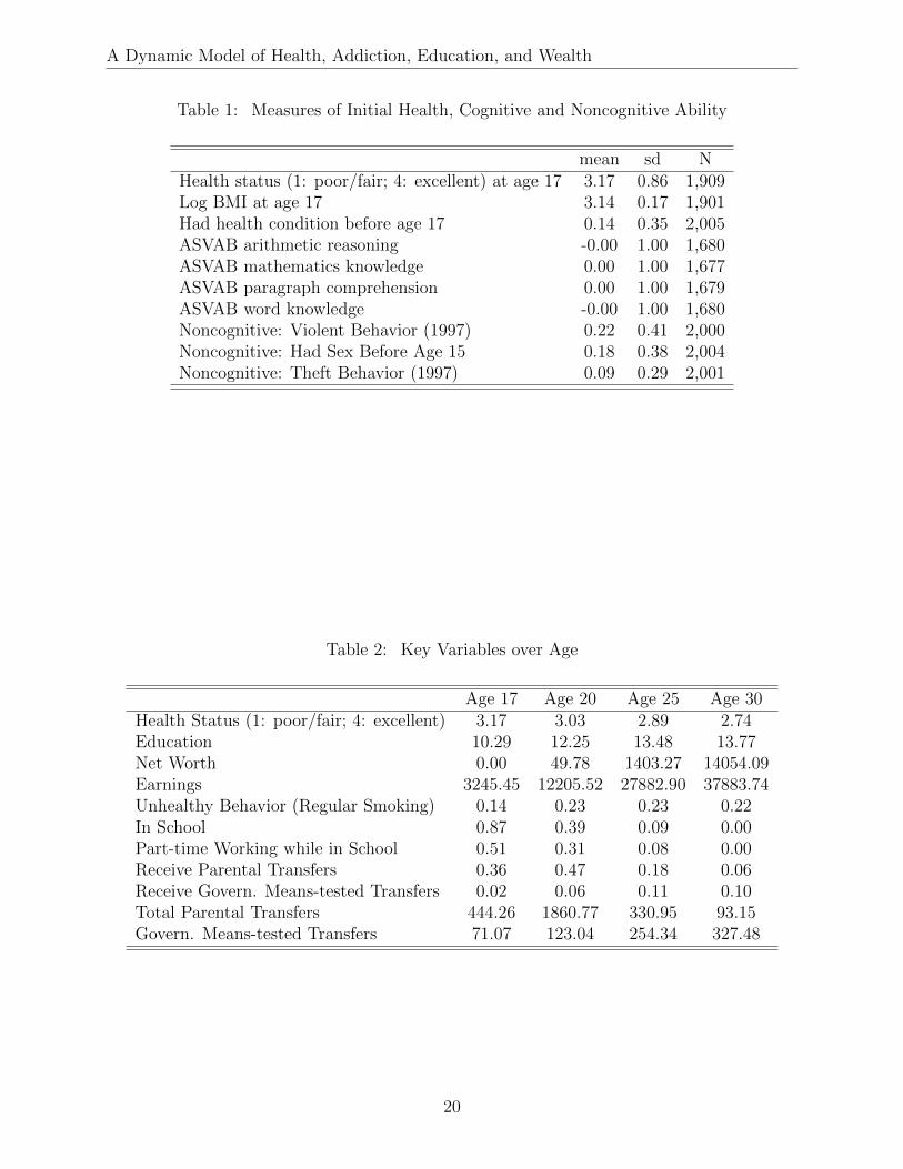
Measures of health, cognitive ability, and noncognitive ability at age 17 are presented in
Table 1. Table 2 reports the statistics of key variables over age groups. The average health,
measured by self-reported health status, is deteriorating over age. Individuals’ average years
of schooling (education) increases from 10.29 at age 17 to 13.77 at age 30. The average net
worth increase from $50 at age 20 to $14,054 at age 30. At age 17, only 14% of the youth
engages in unhealthy behavior (measured by regular smoking); this ratio first increases and
peaks at age 23, then steadily decreases to 22% at age 30.32 At age 17, 87% of the youth
are enrolled in school and the fraction of the youth in school decreases to 3% at age 30.
All nominal variables are in 2004 dollars. The summary statistics for the entire sample is
reported in Web Appendix Table A3.
Education is generally positively correlated with good health and more wealth. As shown
in Table 3, on average, individuals with higher education have better health and health
behaviors and have higher wages and wealth.33 On the other hand, better initial health
are associated with better adult life outcomes such as higher education and wealth (“reverse
causality”). As seen in Figure 1, education and wealth measured at age 25 to 30 are increasing
functions with initial health (measured by health status) at age 17.
31College financial aid gift includes any financial aid respondents received from relatives and friends thatis not expected to be paid back for each college and term attended in each school year.
32At age 23, 26% of individuals smoke regularly.33Figure A7 in the Web Appendix reports educational gradient in health status, smoking behavior, wages,
and wages for individuals aged 25 to 30.
19
A Dynamic Model of Health, Addiction, Education, and Wealth
Table 1: Measures of Initial Health, Cognitive and Noncognitive Ability
mean sd NHealth status (1: poor/fair; 4: excellent) at age 17 3.17 0.86 1,909Log BMI at age 17 3.14 0.17 1,901Had health condition before age 17 0.14 0.35 2,005ASVAB arithmetic reasoning -0.00 1.00 1,680ASVAB mathematics knowledge 0.00 1.00 1,677ASVAB paragraph comprehension 0.00 1.00 1,679ASVAB word knowledge -0.00 1.00 1,680Noncognitive: Violent Behavior (1997) 0.22 0.41 2,000Noncognitive: Had Sex Before Age 15 0.18 0.38 2,004Noncognitive: Theft Behavior (1997) 0.09 0.29 2,001
Table 2: Key Variables over Age
Age 17 Age 20 Age 25 Age 30Health Status (1: poor/fair; 4: excellent) 3.17 3.03 2.89 2.74Education 10.29 12.25 13.48 13.77Net Worth 0.00 49.78 1403.27 14054.09Earnings 3245.45 12205.52 27882.90 37883.74Unhealthy Behavior (Regular Smoking) 0.14 0.23 0.23 0.22In School 0.87 0.39 0.09 0.00Part-time Working while in School 0.51 0.31 0.08 0.00Receive Parental Transfers 0.36 0.47 0.18 0.06Receive Govern. Means-tested Transfers 0.02 0.06 0.11 0.10Total Parental Transfers 444.26 1860.77 330.95 93.15Govern. Means-tested Transfers 71.07 123.04 254.34 327.48
20

A Dynamic Model of Health, Addiction, Education, and Wealth
Table 3: Education Gradient in Health, Smoking, Wages, and Wealth
HS Dropouts 4-Yr College p-value of DiffHealth Status 2.47 3.15 0.0018.5 ≤ BMI < 30 0.75 0.82 0.00Has Health Condition 0.24 0.18 0.00Regular Smoking 0.51 0.05 0.00Hourly Wage 14.32 21.66 0.00Net Worth (in Thousands) -1.19 9.00 0.00
Data source: NLSY97 white males aged 25 to 30.
Health status is measured on the scale of 1 (poor/fair) to 4 (excellent). Health condition is adummy variable for having at least a chronic condition (including cardiovascular condition, heartcondition, asthma, anemia, diabetes, cancer, epilepsy, mental/emotional problems, and eatingdisorders).
(a) Education & Initial Health
11
12
13
14
15
Edu
catio
n (a
ge 2
5 to
30)
Poor/Fair Good Very good ExcellentHealth Status (1: poor/fair; 4: excellent)
(b) Net Worth & Initial Health
-5000
0
5000
10000
15000
Net
Wor
th (a
ge 2
5 to
30)
Poor/Fair Good Very good ExcellentHealth Status (1: poor/fair; 4: excellent)
Figure 1: Initial Health and Education and Net Worth
Health outcomes in adulthood also positively correlated with his parents’ education and
wealth.34 There is a positive correlation between parental education and wealth and the
child’s education and health. As seen in Web Appendix Figures A4 and A5, even after
controlling for measures of the youths’ own cognitive ability, there is still a strong positive
correlation between parents’ education and net worth and an individual’s college attendance
and 4-year college completion.
34See Figure A3 in the Web Appendix.
21
A Dynamic Model of Health, Addiction, Education, and Wealth
4 Empirical Strategy
We estimate a fully parametric model. We present the parametric specifications in Sec-
tion 4.1. 35 In Section 4.2, we discuss the parameters that are identified using externally
supplied data. We then discuss our model identification (Section 4.3) and our method of
estimation (Section 4.4).
4.1 Model Parameterization
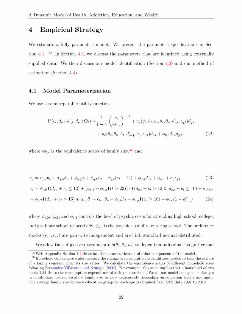
We use a semi-separable utility function
U(ct, dq,t, de,t, dp,t; Ωt) =1
1− γ
(ct
est,e
)1−γ
+ uq(qt, ht, et, θc, θn, de,t, εq,t)dq,t
+ ue(θc, θn, ht, det−1, ep, εe,t)de,t + φk,ede,tdp,t (22)
where est,e is the equivalence scales of family size,36 and
uq = αq,cθc + αq,nθn + φq,qqt + φq,hht + φq,e(et − 12) + φq,dde,t + φq,0 + σqεq,t (23)
ue = φe,01(de,t + et ≤ 12) + (φe,1 + φe,a1(t > 22)) · 1(de,t + et > 12 & de,t + et ≤ 16) + σeεe,t
+ φe,21(de,t + et > 16) + αe,cθc + αe,nθn + φe,hht + φe,p1(ep ≥ 16)− φe,e(1− det−1) (24)
where φe,0, φe,1, and φe,2 controls the level of psychic costs for attending high school, college,
and graduate school respectively, φe,e is the psychic cost of re-entering school. The preference
shocks (εq,t, εe,t) are pair-wise independent and are i.i.d. standard normal distributed.
We allow the subjective discount rate ρ(θc, θn, ht) to depend on individuals’ cognitive and
35Web Appendix Section 1.2 describes the parameterization of other components of the model.36Household equivalence scales measure the change in consumption expenditures needed to keep the welfare
of a family constant when its size varies. We calculate the equivalence scales of different household sizesfollowing Fernandez-Villaverde and Krueger (2007). For example, this scale implies that a household of twoneeds 1.34 times the consumption expenditure of a single household. We do not model endogenous changesin family size; instead we allow family size to vary exogenously depending on education level e and age t.The average family size for each education group for each age is obtained from CPS data 1997 to 2012.
22
A Dynamic Model of Health, Addiction, Education, and Wealth
noncognitive skills and their health,
ρ(θc, θn, ht) = ρ0(1− ρcθc − ρnθn − ρhht), (25)
Therefore the associated subjective discount factor is exp(−ρ0(1− ρcθc − ρnθn − ρhht)).
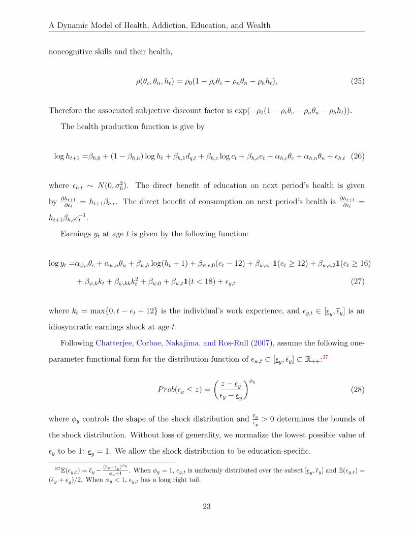
The health production function is give by
log ht+1 =βh,0 + (1− βh,h) log ht + βh,1dq,t + βh,c log ct + βh,eet + αh,cθc + αh,nθn + εh,t (26)
where εh,t ∼ N(0, σ2h). The direct benefit of education on next period’s health is given
by ∂ht+1
∂et= ht+1βh,e. The direct benefit of consumption on next period’s health is ∂ht+1
∂ct=
ht+1βh,cc−1t .
Earnings yt at age t is given by the following function:
log yt =αψ,cθc + αψ,nθn + βψ,h log(ht + 1) + βψ,e,0(et − 12) + βw,e,11(et ≥ 12) + βw,e,21(et ≥ 16)
+ βψ,kkt + βψ,kkk2t + βψ,0 + βψ,t1(t < 18) + εy,t (27)
where kt = max0, t − et + 12 is the individual’s work experience, and εy,t ∈ [εy, εy] is an
idiosyncratic earnings shock at age t.
Following Chatterjee, Corbae, Nakajima, and Ros-Rull (2007), assume the following one-
parameter functional form for the distribution function of εw,t ⊂ [εy, εy] ⊂ R++:37
Prob(εy ≤ z) =
(z − εyεy − εy
)φy(28)
where φy controls the shape of the shock distribution and εyεy> 0 determines the bounds of
the shock distribution. Without loss of generality, we normalize the lowest possible value of
εy to be 1: εy = 1. We allow the shock distribution to be education-specific.
37E(εy,t) = εy−(εy−εy)
φy
φy+1 . When φy = 1, εy,t is uniformly distributed over the subset [εy, εy] and E(εy,t) =
(εy + εy)/2. When φy < 1, εy,t has a long right tail.
23
A Dynamic Model of Health, Addiction, Education, and Wealth
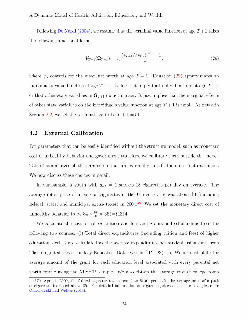
Following De Nardi (2004), we assume that the terminal value function at age T +1 takes
the following functional form:
VT+1(ΩT+1) = φs(sT+1/esT,e)
1−γ − 1
1− γ, (29)
where φs controls for the mean net worth at age T + 1. Equation (29) approximates an
individual’s value function at age T + 1. It does not imply that individuals die at age T + 1
or that other state variables in ΩT+1 do not matter. It just implies that the marginal effects
of other state variables on the individual’s value function at age T + 1 is small. As noted in
Section 2.2, we set the terminal age to be T + 1 = 51.
4.2 External Calibration
For parameters that can be easily identified without the structure model, such as monetary
cost of unhealthy behavior and government transfers, we calibrate them outside the model.
Table 4 summarizes all the parameters that are externally specified in our structural model.
We now discuss these choices in detail.
In our sample, a youth with dq,t = 1 smokes 18 cigarettes per day on average. The
average retail price of a pack of cigarettes in the United States was about $4 (including
federal, state, and municipal excise taxes) in 2004.38 We set the monetary direct cost of
unhealthy behavior to be $4 ×1820× 365=$1314.
We calculate the cost of college tuition and fees and grants and scholarships from the
following two sources: (i) Total direct expenditures (including tuition and fees) of higher
education level et are calculated as the average expenditures per student using data from
The Integrated Postsecondary Education Data System (IPEDS); (ii) We also calculate the
average amount of the grant for each education level associated with every parental net
worth tercile using the NLSY97 sample. We also obtain the average cost of college room
38On April 1, 2009, the federal cigarette tax increased to $1.01 per pack, the average price of a packof cigarettes increased above $5. For detailed information on cigarette prices and excise tax, please seeOrzechowski and Walker (2014).
24

A Dynamic Model of Health, Addiction, Education, and Wealth
Table 4: Parameters Calibrated Outside the Structural Model
Description Parameter Value Source
Direct Cost of UnhealthyBehavior
pq $1314 a pack of cigarettes $4.0
College Tuition & Feestc(e = 13, 14) $5073 IPEDS data on average tuition and fees
1999-2006.tc(e ≥ 15) $10653
College Grants andScholarship
gr(e = 13, 14, sp = T1) $2581
NLSY97 data on average grants andscholarship by years of schooling andparental wealth terciles.
gr(e = 13, 14, sp = T2) $2287gr(e = 13, 14, sp = T3) $2476gr(e ≥ 15, sp = T1) $3604gr(e ≥ 15, sp = T2) $2569gr(e ≥ 15, sp = T3) $2607
College Room and Board tr(e = 13, 14) $4539 Johnson (2013) room and board for 2-yearcollege and 4-year collegetr(e ≥ 15) $6532
GSL Borrowing FlowAnnual
lg(e = 13) $2625
Annual Stafford loan limits 1993 to 2007lg(e = 14) $3500lg(e = 15, 16) $5500lg(e > 16) $8500
GSL Borrowing AggregateLimit
Lg(et ≥ 13 & et ≤ 16) $23000 Undergraduate
Lg(et ≥ 16) $65500 Graduate + Undergraduate
Borrowing Interest Rate rb 5% Federal Student AidLending Interest Rate rl 1% Average real interest rate on 1-year
U.S. government bonds from 2001 to2007
Parental TransferFunction
trp(ep, sp, de,t, et, t) TableA7
NLSY97 sample
Parents ConsumptionSubsidy
trc,t = χ · 1(t < 18) $7800 Kaplan (2012) & Johnson (2013)
Minimum ConsumptionFloor
cmin $2800 NLSY sample average means-testedtransfers among recipients
Risk Aversion Coefficient γ 2.00 Lochner and Monge-Naranjo (2012b)and Johnson (2013)
Terminal Value function φs 1.69 PSID 1999-2011:Median(s51/c50)=1.30
IPEDS = Integrated Postsecondary Education Data System. Average tuition and fees are weighted by full-time enrollment and are deflated in 2004 dollars. Because expenditures are higher at four-year institutionsthan at two-year institutions, there is a noticeable jump in cost between two and three years of college.Within our sample period, the aggregate subsidized Stafford Loan Limits is $23000 for undergraduate and$65500 for graduate and undergraduate in total. The Interest rate ranges from 3.34 to 8.25% for StaffordLoans over the time period 1997 to 2011. Parental consumption subsidy is given by trc,t = χ · 1(t < 18),where χ is the value of direct consumption subsidy provided by the parents such as shared housing and mealswhen the youth attends high school.
25
A Dynamic Model of Health, Addiction, Education, and Wealth
and board from IPEDS for two year college and 4 year college, respectively. We set the
borrowing interest rate equal to 5 percent annually. We set the lending interest rate rl to be
1 percent annually, which is the average real interest rate on 1-year U.S. government bonds
from 2001 to 2007.
We estimate the logarithm of parental monetary transfers, log(trp,t+1) using our NLSY97
sample (see Section 1.2 in the Web Appendix for parameterization); the parameter estimates
are reported in Web Appendix Table A7. In the sample, 94% of youth who are attending
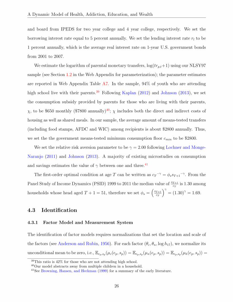
high school live with their parents.39 Following Kaplan (2012) and Johnson (2013), we set
the consumption subsidy provided by parents for those who are living with their parents,
χ, to be $650 monthly ($7800 annually)40; χ includes both the direct and indirect costs of
housing as well as shared meals. In our sample, the average amount of means-tested transfers
(including food stamps, AFDC and WIC) among recipients is about $2800 annually. Thus,
we set the the government means-tested minimum consumption floor cmin to be $2800.
We set the relative risk aversion parameter to be γ = 2.00 following Lochner and Monge-
Naranjo (2011) and Johnson (2013). A majority of existing microstudies on consumption
and savings estimates the value of γ between one and three.41
The first-order optimal condition at age T can be written as cT−γ = φssT+1
−γ. From the
Panel Study of Income Dynamics (PSID) 1999 to 2011 the median value of sT+1
cTis 1.30 among
households whose head aged T + 1 = 51, therefore we set φs =(sT+1
cT
)γ= (1.30)γ = 1.69.
4.3 Identification
4.3.1 Factor Model and Measurement System
The identification of factor models requires normalizations that set the location and scale of
the factors (see Anderson and Rubin, 1956). For each factor (θc, θn, log h17), we normalize its
unconditional mean to be zero, i.e., Eep,sp(µc(ep, sp)) = Eep,sp(µn(ep, sp)) = Eep,sp(µh(ep, sp)) =
39This ratio is 42% for those who are not attending high school.40Our model abstracts away from multiple children in a household.41See Browning, Hansen, and Heckman (1999) for a summary of the early literature.
26

A Dynamic Model of Health, Addiction, Education, and Wealth
0, and standard deviation to be one, i.e., σc = σn = σh = 1.42
4.3.2 Dynamic Model and Structure Parameters
Our identification strategy relies on the analysis of Heckman and Navarro (2007) and Heck-
man, Humphries, and Veramendi (2016b). In particular, under the assumption that εy,t are
i.i.d, the structural parameters in the earnings function are identified by using the factors
scores of unobserved factors in the first stage estimation. The parameters in the health
production function are also identified using factors scores from the first stage.
The parameters of the subjective discount rate are identified by consumption growth.
To illustrate, let us consider the Euler equation under CRRA utility specification for those
who are far away from borrowing constraints (abstracting away from uncertainty and health
production):43
γ · (log ct+1 − log ct) = −ρ(θc, θn, ht) + log(1 + r).
where γ is the relative risk aversion coefficient. Though we do not directly observe con-
sumption growth in our data, we do observe individuals’ net worth and income and thus can
construct the implied consumption growth using our model’s budget constraint equations
(Equations 9 and 11).
The identification of preference parameters on addiction and the depreciation rate is
based on the following regression:
dq,t =bq,0 + bq,1dq,t−1 + bq,2dq,t−2 + bq,eet
+ bq,c · (measure of θc) + bq,n · (measure of θn) + bq,h · (measure of ht) +Xtβ + error termt.
The regression coefficient bq,1 identifies the slope parameter of addiction stock qt = dq,t−1 +
42Therefore, E(h17) = exp(0.5) = 1.6487 and SD(h17) =√
(exp(1)− 1) · exp(0.5) = 2.1612.43For illustrative purposes, here we assume uc(ct; Ωt) = c1−γt /1− γ and r is the borrowing/lending interest
rate.
27
A Dynamic Model of Health, Addiction, Education, and Wealth
(1−δq)qt−2 in the preference function (∂uq/∂qt = φq,q) and bq,2 then identifies the depreciation
rate of the addiction stock δq.
4.4 Estimation Method
We use a two-step estimation procedure to estimate the structural model parameters. In the
first step, we estimate the parameters on the measurement system and the joint distribu-
tion of health, and cognitive and noncognitive ability at age 17 using simulated maximum
likelihood estimation.
max Πi
∫θc,θn,log(h17)
f(Zi;Xi, θc, θn, log(h17))dF (θc, θn, log(h17))
In the second step, we use the method of simulated moments to estimate parameters
on individuals’ preferences, production function on health and human capital, and discount
factors.44 The initial conditions for health and cognitive and noncognitive ability in the
second step are obtained by simulation using the parameter estimates from the first step.
In total, we estimate 59 parameters in the second step. The targeted moments are listed in
Table 5. There are three types of targeted moments: (i) choice probabilities (on schooling and
engaging unhealthy behavior) and outcome variables (earnings) for every age; (ii) covariance
terms from regression analysis for savings, health status transition, log wage, probabilities
of schooling and engaging unhealthy behavior (“indirect inference”), and (iii) average net
worth, health status, and earnings by different education categories.
5 Estimation Results
This section discusses our estimates. Sections 5.1 and 5.2 discusses the parameter estimates
and the goodness of model fit respectively. Section 5.3 discuss the sorting pattern into
44The choice variables in the model include not only discrete controls such as schooling and unhealthybehavior but also continuous controls such as asset level. As a result, we use Simulated Method of Moments(SMM) to estimate the model.
28

A Dynamic Model of Health, Addiction, Education, and Wealth
Table 5: Targeted Moments for SMM Estimation
Targeted Moments # MomentsChoice probabilities, state variables, and outcome variables over the life-cycleProbability of engaging unhealthy behavior for each age 17 to 30 14Probability of schooling for each age 17 to 27 11Average log earnings for each age 17 to 30 14Average net worth at ages 20, 25, and 30 3Average years of schooling, health status, years of unhealthy behavior at age 30 3Variance of log years of schooling, log health status, log years of unhealthy behavior,log earnings at age 30
4
Probabilities of high school graduation, some college, and 4-year college at ages 25and 30
6
Probability of enrolling in college at age 21 1Probability of graduating from 4-year college at age 25 1Probability of part-time working while in school 1Average log earnings when working part-time while in school 1Conditional moments for each of the 4 education categoriesAverage net worth at age 25 and age 30 4 × 2Average negative net worth at age 25 and age 30 4 × 2Average health status at age 25 and age 30 4 × 2Average years of unhealthy behavior at age 25 and age 30 4 × 2Average earnings at age 25 and age 30 4 × 2Average log earnings at age 25 and age 30 4 × 2Top 5 percentile of log earnings at age 25 and age 30 4 × 2Standard deviation of log earnings at age 25 and age 30 4 × 2Covariance terms from auxiliary models (Indirect Inference)Regression coefficients of log earnings on years worked, years worked squared, years ofschooling, high school graduate, some college, 4-year college, cognitive ability, cogni-tive ability × 4-year college, noncognitive ability, noncognitive ability × 4-year college,health status, health status × 4-year college
12
Regression coefficients of next period’s health status on current health status, un-healthy behavior, log earnings, years of schooling, cognitive ability, noncognitive abil-ity
6
Regression coefficients of log savings on cognitive ability, noncognitive ability, healthstatus, log earnings, age > 20, age > 25
6
Regression coefficients of school enrollment on parents’ education, parents net worth,cognitive ability, noncognitive ability, age, age 17 dummy, health status, previousperiod’s enrollment status
5
Regression coefficients of unhealthy behavior on unhealthy behavior at t−1, unhealthybehavior at t − 2, years of schooling, cognitive ability, noncognitive ability, healthstatus, log earnings
7
29
A Dynamic Model of Health, Addiction, Education, and Wealth
education based on unobserved initial health, cognitive ability, and noncognitive ability.
Section 5.4 evaluates the direct benefits of health on schooling. Section 5.5 compares our
benchmark model of rational addiction with a behavior model of myopic unhealthy behavior.
5.1 Parameter Estimates
5.1.1 Measurement System
The initial distribution of (θc, θn, log(h17)) is reported in Table B8. Individuals whose parents
have higher education and wealth on average have higher initial endowment in cognitive
ability, noncognitive ability, and initial health. These three initial endowments are positively
correlated with each other.45 The correlation between cognitive ability and noncognitive
ability is moderate (0.285).46 The correlation between cognitive ability and log health at age
17 is much smaller (0.137), and the correlation between noncognitive ability and log health
at age 17 is relatively high (0.461). The parameter estimates of the measurement equations
are reported in appendix Table B9.
5.1.2 Structural Model Parameters: Subjective Discount Rate, Health Dynam-
ics, Earnings Dynamics, and Preferences
Table B10 reports parameter estimates for the earnings equation. Table B11 reports es-
timated parameter values for health production function. Higher education improves the
growth rate of health. Higher consumption also promotes better health but at a decreasing
rate. Engaging in unhealthy behavior has a sizable negative impact on the growth rate
of health. Finally, both cognitive ability and noncognitive ability have positive impact on
health production.
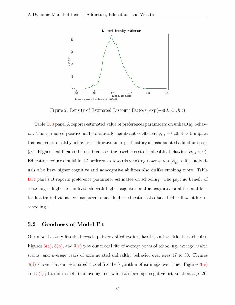
Parameter estimates of discount rate are reported in Table B12. Figure 2 plots the
density of estimated discount factors in the baseline model for individuals aged 17 to 30.
The estimated discount factors range from 0.93 to 0.98.
45The variance of each factor is normalized to one for identification.46Heckman, Humphries, and Veramendi (2016a) report an estimate of .40 for a related model.
30
A Dynamic Model of Health, Addiction, Education, and Wealth
020
4060
80D
ensi
ty
.94 .95 .96 .97 .98 .99 Discount Factor
kernel = epanechnikov, bandwidth = 0.0004
Kernel density estimate
Figure 2: Density of Estimated Discount Factors: exp(−ρ(θc, θn, ht))
Table B13 panel A reports estimated value of preferences parameters on unhealthy behav-
ior. The estimated positive and statistically significant coefficient φq,q = 0.0051 > 0 implies
that current unhealthy behavior is addictive to its past history of accumulated addiction stock
(qt). Higher health capital stock increases the psychic cost of unhealthy behavior (φq,h < 0).
Education reduces individuals’ preferences towards smoking downwards (φq,e < 0). Individ-
uals who have higher cognitive and noncogntive abilities also dislike smoking more. Table
B13 panels B reports preference parameter estimates on schooling. The psychic benefit of
schooling is higher for individuals with higher cognitive and noncognitive abilities and bet-
ter health; individuals whose parents have higher education also have higher flow utility of
schooling.
5.2 Goodness of Model Fit
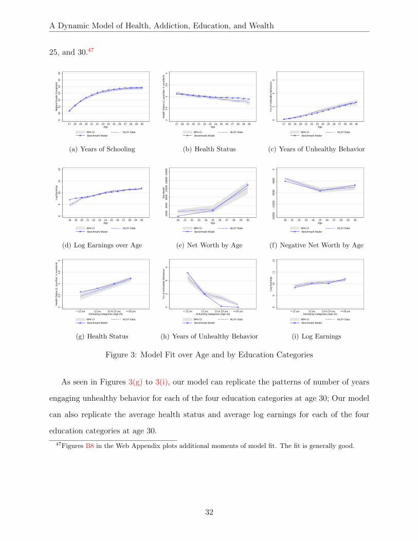
Our model closely fits the lifecycle patterns of education, health, and wealth. In particular,
Figures 3(a), 3(b), and 3(c) plot our model fits of average years of schooling, average health
status, and average years of accumulated unhealthy behavior over ages 17 to 30. Figures
3(d) shows that our estimated model fits the logarithm of earnings over time. Figures 3(e)
and 3(f) plot our model fits of average net worth and average negative net worth at ages 20,
31
A Dynamic Model of Health, Addiction, Education, and Wealth
25, and 30.479
1011
1213
1415
16 H
ighe
st G
rade
Com
plet
ed
17 18 19 20 21 22 23 24 25 26 27 28 29 30 Age
99% CI NLSY Data Benchmark Model
(a) Years of Schooling
22.
53
3.5
4 H
ealth
Sta
tus
(1: p
oor/
fair;
4: e
xcel
lent
)
17 18 19 20 21 22 23 24 25 26 27 28 29 30 Age
99% CI NLSY Data Benchmark Model
(b) Health Status
02
46
Yrs
of U
nhea
lthy
Beh
avio
rs
17 18 19 20 21 22 23 24 25 26 27 28 29 30 Age
99% CI NLSY Data Benchmark Model
(c) Years of Unhealthy Behavior
89
1011
12 L
og E
arni
ngs
18 19 20 21 22 23 24 25 26 27 28 29 30 Age
99% CI NLSY Data Benchmark Model
(d) Log Earnings over Age
-150
035
0085
0013
500
1850
023
500
Net
Wor
th
20 21 22 23 24 25 26 27 28 29 30 Age
99% CI NLSY Data Benchmark Model
(e) Net Worth by Age
-160
00-1
2000
-800
0-4
000
0
20 21 22 23 24 25 26 27 28 29 30 Age
99% CI NLSY Data Benchmark Model
(f) Negative Net Worth by Age
22.
53
3.5
4 H
ealth
Sta
tus
(1: p
oor/
fair;
4: e
xcel
lent
)
< 12 yrs 12 yrs 13 to 15 yrs >=16 yrs Schooling Categories (Age 25)
99% CI NLSY Data Benchmark Model
(g) Health Status
02
46
Yrs
of U
nhea
lthy
Beh
avio
rs
< 12 yrs 12 yrs 13 to 15 yrs >=16 yrs Schooling Categories (Age 25)
99% CI NLSY Data Benchmark Model
(h) Years of Unhealthy Behavior
89
1011
12 L
og E
arni
ngs
< 12 yrs 12 yrs 13 to 15 yrs >=16 yrs Schooling Categories (Age 25)
99% CI NLSY Data Benchmark Model
(i) Log Earnings
Figure 3: Model Fit over Age and by Education Categories
As seen in Figures 3(g) to 3(i), our model can replicate the patterns of number of years
engaging unhealthy behavior for each of the four education categories at age 30; Our model
can also replicate the average health status and average log earnings for each of the four
education categories at age 30.
47Figures B8 in the Web Appendix plots additional moments of model fit. The fit is generally good.
32

A Dynamic Model of Health, Addiction, Education, and Wealth
5.3 Sorting into Education Based on Early Endowments0
.2.4
.6D
ensity
−2 −1 0 1 Log Health at Age 17
< 12 yrs 12 yrs
13 to 15 yrs >=16 yrs
0.1
.2.3
.4.5
Density
−4 −2 0 2 4 Cognitive Ability
< 12 yrs 12 yrs
13 to 15 yrs >=16 yrs
0.2
.4.6
Density
−4 −2 0 2 Noncognitive Ability
< 12 yrs 12 yrs
13 to 15 yrs >=16 yrs
Figure 4: Density of Early Endowments Conditional on Age-30 Education
Using simulated data based on estimated model parameters, we now illustrate the magnitude
of sorting into education at age 30 based on unobserved ability and initial health capital stock.
Figure 4 is the density plot of three unobservables by education groups in the simulated data.
As we can see, based on cognitive and noncognitive ability and initial health capital stock,
individuals sort into different education categories.
5.4 Evaluating Direct Benefits of Health on Schooling
910
1112
1314
1516
Hig
hest
Gra
de C
ompl
eted
17 18 19 20 21 22 23 24 25 26 27 28 29 30Age
Benchmark Model CF: Removing Health Benefit from Psychic Cost of Schooling
(a) Education
0.1
.2.3
.4.5
.6.7
.8.9
1 C
olle
ge A
ttend
ance
1 2 3 4 Cognitive Ability Quartiles
Benchmark Model CF: Removing Health Benefit from Psychic Cost of Schooling
(b) College Attendance (Age 21)
0.1
.2.3
.4.5
.6.7
.8.9
1 4
-Yr
Col
lege
Gra
duat
ion
1 2 3 4 Cognitive Ability Quartiles
Benchmark Model CF: Removing Health Benefit from Psychic Cost of Schooling
(c) 4-Year College Graduation (Age25)
Figure 5: Economic Implications: Removing Direct Benefits of Health on Schooling (φe,h = 0)
In our model, health can directly affect an individual’s educational decision by reducing
his psychic cost associated with schooling (φe,h = 0.0494 > 0).48 To evaluate the direct ben-
efit of health on education, we shut down the preference parameter on schooling associated
48Health can also indirectly impact educational choices through its effects on wage equation and subjectivediscount factor.
33

A Dynamic Model of Health, Addiction, Education, and Wealth
with health, i.e., we set φe,h = 0. The result is reported in Figure 5. As we can see in
Figure 5, removing the direct benefits of health on schooling reduces both the rate of college
enrollment and the rate of 4-year college graduation.49
5.5 A Comparison with A Behavior Model with Myopic Unhealthy
Behavior
0.1
.2.3
.4 U
nhea
lthy
Beh
avio
r
17 20 23 26 29 32 35 38 41 44 47 50Age
Benchmark Model CF: Behavior Model with Myopic Unhealthy Behavior
(a) Unhealthy Behavior Probability
02
46
Yrs
of U
nhea
lthy
Beh
avio
rs
1 2 3 4Schooling Categories (Age 30)
Benchmark Model CF: Behavior Model with Myopic Unhealthy Behavior
(b) Yrs of Unhealthy Behavior by Education (Age30)
Figure 6: Forward-looking Unhealthy Behavior vs Myopic Unhealthy Behavior
In this section we compare our model to a counterfactual model where individuals make
myopic decisions on their unhealthy behavior. Recall individuals’ optimal decisions in our
dynamic benchmark model is given by Equation 17. However, in a model with myopic
unhealthy behavior, an individual chooses dq,t = 1 if and only if U∗(dq,t = 1; Ωt) > U∗(dq,t =
0; Ωt).50
As seen in Figure 6, compared with our benchmark model with rational addiction (i.e.,
the fitted model), the predicted probability of unhealthy behavior is much larger in the model
with myopic unhealthy behavior because individuals do not take into account the negative
health capital effect. More importantly, our benchmark model predicts the probability of
49In our model, the direct benefit of health on education is through its effects on whether to attend schoolnext year, i.e., when to stop investing in education. In future research, we can also allow health to affectone’s education outcome by affecting one’s academic test score and college major choices.
50Individuals’ decisions on education, savings, and working are still forward-looking.
34

A Dynamic Model of Health, Addiction, Education, and Wealth
unhealthy behavior decreases at the later ages as individuals’ health deteriorates and the
marginal productivity value of health becomes larger, whereas the myopic model does not.51
Finally, compared to the benchmark model, the predicted increases in unhealthy behavior
in the myopic model are concentrated among the low educated individuals.
6 Policy Experiments
Table 6: Health, Education, Wealth, and Consumption under Different Experiments
Benchmark Excise Tax Early Endowment
Predicted Changes (%)
Avg years of schooling at age 30 13.8654 0.10 0.24
Avg health capital at age 30 1.5432 0.50 0.57
Avg addiction stock at age 30 0.4750 -10.38 -6.22
Avg earnings at age 30 46393.2536 0.16 0.43
Avg consumption at age 30 43320.0294 -0.03 0.50
Avg net worth at age 30 15717.7701 0.66 1.07
Var of log years of schooling at age 30 0.0525 -0.03 -1.27
Var of log health at age 30 1.9541 -0.68 -0.41
Var of log earnings at age 30 0.7770 -0.05 -0.45
Var of log consumption at age 30 0.3829 0.87 -1.37
Gini of net worth at age 30 1.3321 -0.02 -0.57
Gini of earnings at age 30 0.4704 -0.04 -0.25
51Though one can always artificially introduce an age-squared term into the preference function of un-healthy behavior to “fit” the downward trend at later ages in the myopic model, however such practice ismechanical and does not lend us insight about the economic determinants behind the observed life-cyclepattern of unhealthy behavior.
35
A Dynamic Model of Health, Addiction, Education, and Wealth
0.1
.2.3
.4 U
nhea
lthy
Beh
avio
r
17 18 19 20 21 22 23 24 25 26 27 28 29 30Age
Benchmark Model CF: Increasing Excise Tax in Benchmark Model
0.0
5.1
.15
Initi
ate
Sm
okin
g
17 18 19 20 21 22 23 24 25 26 27 28 29 30Age
Benchmark Model CF: Increasing Excise Tax in Benchmark Model
Figure 7: Effects of Increasing Revenue-Neutral Excise Tax
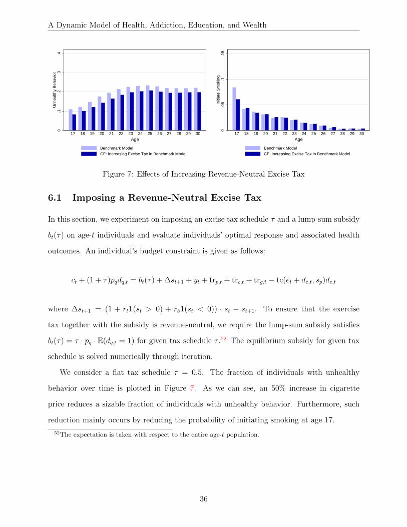
6.1 Imposing a Revenue-Neutral Excise Tax
In this section, we experiment on imposing an excise tax schedule τ and a lump-sum subsidy
bt(τ) on age-t individuals and evaluate individuals’ optimal response and associated health
outcomes. An individual’s budget constraint is given as follows:
ct + (1 + τ)pqdq,t = bt(τ) + ∆st+1 + yt + trp,t + trc,t + trg,t − tc(et + de,t, sp)de,t
where ∆st+1 = (1 + rl1(st > 0) + rb1(st < 0)) · st − st+1. To ensure that the exercise
tax together with the subsidy is revenue-neutral, we require the lump-sum subsidy satisfies
bt(τ) = τ · pq · E(dq,t = 1) for given tax schedule τ .52 The equilibrium subsidy for given tax
schedule is solved numerically through iteration.
We consider a flat tax schedule τ = 0.5. The fraction of individuals with unhealthy
behavior over time is plotted in Figure 7. As we can see, an 50% increase in cigarette
price reduces a sizable fraction of individuals with unhealthy behavior. Furthermore, such
reduction mainly occurs by reducing the probability of initiating smoking at age 17.
52The expectation is taken with respect to the entire age-t population.
36
A Dynamic Model of Health, Addiction, Education, and Wealth
6.2 Improving Early Endowment
In this section we consider an early intervention program that increases adolescent cognitive
ability and noncogntive ability among the most disadvantaged youths. In particular, we
increase both the cognitive and noncognitive abilities by 0.1 standard deviation for the
youths whose cognitive and noncogntive abilities are lower than -0.7 standard deviation (i.e.,
θc < −0.7 and θn < −0.7); these youths belongs to the bottom 10% of the population.
As seen in the second column of Table 6, compared to the benchmark model, the average
years of schooling increases by 0.24% (0.03 years). The average health capital increases by
0.57%, while the average addiction stock reduced by 6.22%. Improving early endowments
also leads to 0.43% increases in average earnings, 0.50% increases in average consumption,
and 1.07% increase in average net worth at age 30.
Under this policy experiment, the inequality measures in years of schooling, health, earn-
ings, and consumption are reduced. However, the variance of log addiction stock at age 30
increases in this experiment. The Gini coefficients of net worth and earnings at age 30 are
also reduced.
7 Conclusion
We develop and structurally estimate a life cycle model with endogenous decisions on health,
education, and wealth. Using this estimated model, we evaluate the dynamic economic
mechanisms through which health, education, and wealth impact each other. We also use
the estimated model to conduct counterfactual analysis on revenue-neutral excise tax and
early childhood intervention.
With the development of our model we hope to lay down a framework to investigate other
applied questions on the origins of inequality in health and human capital and their dynamic
relationships over the life cycle. There are two possible future research directions. First, our
model can be extended to study questions on intergenerational mobility. In particular, we
37
A Dynamic Model of Health, Addiction, Education, and Wealth
can introduce overlapping generations into our model and investigate the parents’ optimal
investment decisions for their children. Second, our model can be directly extended to study
life cycle inequality in health, education, and wealth by race. In particular, we can investigate
the racial disparity in education, health, and wealth by evaluating the different impacts
resulting from the racial differences in offered wages, subjective discount rates, preferences
over schooling, employment, and unhealthy behavior, and heath production functions.
38

A Dynamic Model of Health, Addiction, Education, and Wealth
References
Adda, Jerome, and Francesca Cornaglia, 2006, Taxes, Cigarette Consumption, and Smoking
Intensity, The American Economic Review 96, pp. 1013–1028.
Anderson, T. W., and Herman Rubin, 1956, Statistical Inference in Factor Analysis, in
Proceedings of the Third Berkeley Symposium on Mathematical Statistics and Probability,
Volume 5: Contributions to Econometrics, Industrial Research, and Psychometry pp. 111–
150 Berkeley, Calif. University of California Press.
Bailey, Martha J., and Susan M. Dynarski, 2011, Gains and Gaps: Changing Inequality in
U.S. College Entry and Completion, NBER Working Paper No. w17633.
Becker, Gary S., Michael Grossman, and Kevin M. Murphy, 1991, Rational Addiction and
the Effect of Price on Consumption, The American Economic Review 81, pp. 237–241.
Becker, Gary S., Michael Grossman, and Kevin M. Murphy, 1994, An Empirical Analysis of
Cigarette Addiction, The American Economic Review 84, pp. 396–418.
Becker, Gary S., and Kevin M. Murphy, 1988, A Theory of Rational Addiction, Journal of
Political Economy 96, pp. 675–700.
Belley, Philippe, and Lance Lochner, 2007, The Changing Role of Family Income and Ability
in Determining Educational Achievement, Journal of Human Capital 1, pp. 37–89.
Browning, Martin, Lars Peter Hansen, and James J. Heckman, 1999, Micro Data and Gen-
eral Equilibrium Models, in John B. Taylor, and Michael Woodford, eds.: Handbook of
Macroeconomics (Elsevier, ).
Cameron, Stephen V., and Christopher Taber, 2004, Estimation of Educational Borrowing
Constraints Using Returns to Schooling, Journal of Political Economy 112, pp. 132–182.
Carneiro, Pedro, and James J. Heckman, 2002, The Evidence on Credit Constraints in Post-
Secondary Schooling, The Economic Journal 112, 705–734.
39
A Dynamic Model of Health, Addiction, Education, and Wealth
Centers for Disease Control and Prevention, 2010, How Tobacco Smoke Causes Disease: The
Biology and Behavioral Basis for Smoking-Attributable Disease, A report of the surgeon
general U.S. Department of Health and Human Services, Centers for Disease Control and
Prevention, National Center for Chronic Disease Prevention and Health Promotion, Office
on Smoking and Health Atlanta, GA.
Chaloupka, Frank, 1991, Rational Addictive Behavior and Cigarette Smoking, Journal of
Political Economy 99, 722–42.
Chatterjee, Satyajit, Dean Corbae, Makoto Nakajima, and Jos-Vctor Ros-Rull, 2007, A
Quantitative Theory of Unsecured Consumer Credit with Risk of Default, Econometrica
75, 1525–1589.
Chen, Lina, George Davey Smith, Robert M. Harbord, and Sarah J. Lewis, 2008, Alcohol In-
take and Blood Pressure: A Systematic Review Implementing a Mendelian Randomization
Approach, PLoS Medicine 5, e52.
Conti, Gabriella, James Heckman, and Sergio Urzua, 2010, The Education-Health Gradient,
The American Economic Review 100, 234–238.
Conti, Gabriella, James J. Heckman, and Sergio Urzua, 2010, The Education-Health Gradi-
ent, American Economic Review: Papers and Proceedings 100, 1–5.
Currie, Janet, 2009, Healthy, Wealthy, and Wise: Socioeconomic Status, Poor Health in
Childhood, and Human Capital Development, Journal of Economic Literature 47, pp.
87–122.
Cutler, David M., and Adriana Lleras-Muney, 2006, Education and Health: Evaluating
Theories and Evidence, Working Paper 12352 National Bureau of Economic Research.
Cutler, David M, and Adriana Lleras-Muney, 2010, Understanding Differences in Health
Behavior by Education, Journal of Health Economics 29, 1–28.
40

A Dynamic Model of Health, Addiction, Education, and Wealth
De Nardi, Mariacristina, 2004, Wealth Inequality and Intergenerational Links, The Review
of Economic Studies 71, 743–768.
De Nardi, Mariacristina, Eric French, and John Bailey Jones, 2009, Life Expectancy and
Old Age Savings, American Economic Review 99, 110–15.
De Nardi, Mariacristina, Eric French, and John B. Jones, 2010, Why Do the Elderly Save?
The Role of Medical Expenses, Journal of Political Economy 118, pp. 39–75.
Deaton, Angus, 2003, Health, Inequality, and Economic Development, Journal of Economic
Literature 41, pp. 113–158.
Deaton, Angus, 2015, The Great Escape: Health, Wealth, and the Origins of Inequality.
(Princeton University Press Princeton, New Jersey).
Dohmen, Thomas, Armin Falk, David Huffman, Uwe Sunde, Jurgen Schupp, and Gert G.
Wagner, 2011, Individual Risk Attitudes: Measurement, Determinants and Behavioral
Consequences, Journal of the European Economic Association 9, 522–550.
Fernandez-Villaverde, Jesus, and Dirk Krueger, 2007, Consumption over the Life Cycle:
Facts from Consumer Expenditure Survey Data, The Review of Economics and Statistics
89, 552–565.
Galama, Titus, 2011, A Contribution to Health Capital Theory, Working Papers 831 RAND
Corporation Publications Department.
Galama, Titus, and Hans van Kippersluis, 2010, A Theory of Socioeconomic Disparities
in Health Over the Life Cycle, Working Papers 773 RAND Corporation Publications
Department.
Goldman, Dana, and James P. Smith, 2011, The Increasing Value of Education to Health,
Social Science and Medicine 72, 1728–1737.
41
A Dynamic Model of Health, Addiction, Education, and Wealth
Grossman, Michael, 1972, On the Concept of Health Capital and the Demand for Health,
The Journal of Political Economy 80, pp. 223–255.
Grossman, Michael, 2008, The Relationship between Health and Schooling, Eastern Eco-
nomic Journal 34, 281–292.
Grossman, Michael, and Frank J. Chaloupka, 1998, The demand for cocaine by young adults:
a rational addiction approach, Journal of Health Economics 17, 427 – 474.
Grossman, Michael, Frank J. Chaloupka, and Ismail Sirtalan, 1998, AN EMPIRICAL ANAL-
YSIS OF ALCOHOL ADDICTION: RESULTS FROM THE MONITORING THE FU-
TURE PANELS, Economic Inquiry 36, 39–48.
Gruber, Jonathan, and Botond Koszegi, 2001, Is Addiction “Rational”? Theory and Evi-
dence, The Quarterly Journal of Economics 116, 1261–1303.
Hai, Rong, and James J. Heckman, 2016, Inequality in Human Capital and Endogenous
Credit Constraints, Under review at Review of Economic Dynamics.
Heckman, James J., John Eric Humphries, and Gregory Veramendi, 2016a, Dynamic Treat-
ment Effects, Journal of Econometrics 191, 276–292.
Heckman, James J., John Eric Humphries, and Gregory Veramendi, 2016b, Returns to
Education: The Causal Effects of Education on Earnings, Health and Smoking, Under
revision, Journal of Political Economy.
Heckman, James J., and Tim Kautz, 2014, Fostering and Measuring Skills: Interventions
That Improve Character and Cognition, in James J. Heckman, John Eric Humphries, and
Tim Kautz, eds.: The Myth of Achievement Tests: The GED and the Role of Character
in American Life (University of Chicago Press, Chicago ).
Heckman, James J., and Stefano Mosso, 2014, The Economics of Human Development and
Social Mobility, Annual Review of Economics 6, 689–733.
42

A Dynamic Model of Health, Addiction, Education, and Wealth
Heckman, James J., and Salvador Navarro, 2007, Dynamic Discrete Choice and Dynamic
Treatment Effects, Journal of Econometrics 136, 341–396.
Johnson, Matthew T., 2013, Borrowing Constraints, College Enrollment, and Delayed Entry,
Journal of Labor Economics 31, pp. 669–725.
Kaplan, Greg, 2012, Moving Back Home: Insurance Against Labor Market Risk, Journal of
Political Economy 120, 446–512.
Kautz, Tim, and Wladimir Zanoni, 2015, Measuring and Fostering Non-Cognitive Skills in
Adolescents: Evidence from Chicago Public Schools and the OneGoal Program, Unpub-
lished manuscript, University of Chicago, Department of Economics.
Keane, Michael P., and Kenneth I. Wolpin, 2001, The Effect of Parental Transfers and
Borrowing Constraints on Educational Attainment, International Economic Review 42,
1051–1103.
Kenkel, Donald S, 1991, Health Behavior, Health Knowledge, and Schooling, Journal of
Political Economy 99, 287–305.
Lochner, Lance, and Alexander Monge-Naranjo, 2012a, Credit Constraints in Education,
Annual Review of Economics 4, 225–256.
Lochner, Lance J., and Alexander Monge-Naranjo, 2011, The Nature of Credit Constraints
and Human Capital, American Economic Review 101, 2487–2529.
Lochner, Lance J., and Alexander Monge-Naranjo, 2012b, Credit Constraints in Education,
Annual Review of Economics 4, 225–256.
McGinnis, J. Michael, Pamela Williams-Russo, and James R. Knickman, 2002, The Case
For More Active Policy Attention To Health Promotion, Health Affairs 21, 78–93.
43
A Dynamic Model of Health, Addiction, Education, and Wealth
Navarro, Salvador, 2011a, Using Observed Choices to Infer Agent’s Information: Reconsid-
ering the Importance of Borrowing Constraints, Uncertainty and Preferences in College
Attendance, Working paper, .
Navarro, Salvador, 2011b, Using Observed Choices to Infer Agent’s Information: Reconsid-
ering the Importance of Borrowing Constraints, Uncertainty and Preferences in College
Attendance, Working Paper 20118, University of Western Ontario, CIBC Centre for Hu-
man Capital and Productivity.
Olekalns, Nilss, and Peter Bardsley, 1996, Rational Addiction to Caffeine: An Analysis of
Coffee Consumption, Journal of Political Economy 104, pp. 1100–1104.
Orzechowski, and Walker, 2014, The Tax Burden on Tabacco, .
Savelyev, Peter A., and Kegon Teng Kok Tan, 2014, Personality, Education, and Health-
Related Outcomes of High-Ability Individuals, Working paper, .
Sloan, Frank A., Jan Ostermann, Christopher Conover, Donald H. Taylor, and Gabriel
Picone, 2004, The Price of Smoking. (MIT Press Cambridge, MA).
Smith, George Davey, 2007, Life-Course Approaches to Inequalities in Adult Chronic Disease
Risk, Proceedings of the Nutrition Society 66, 216–236.
Steinberg, Laurence, 2008, A social neuroscience perspective on adolescent risk-taking, De-
velopmental Review 28, 78–106.
Sundmacher, Leonie, 2012, The effect of health shocks on smoking and obesity, The European
Journal of Health Economics 13, pp. 451–460.
44
A Dynamic Model of Health, Addiction, Education, andWealth
Web Appendix
Rong Hai and James J. Heckman
09/02/2016
1
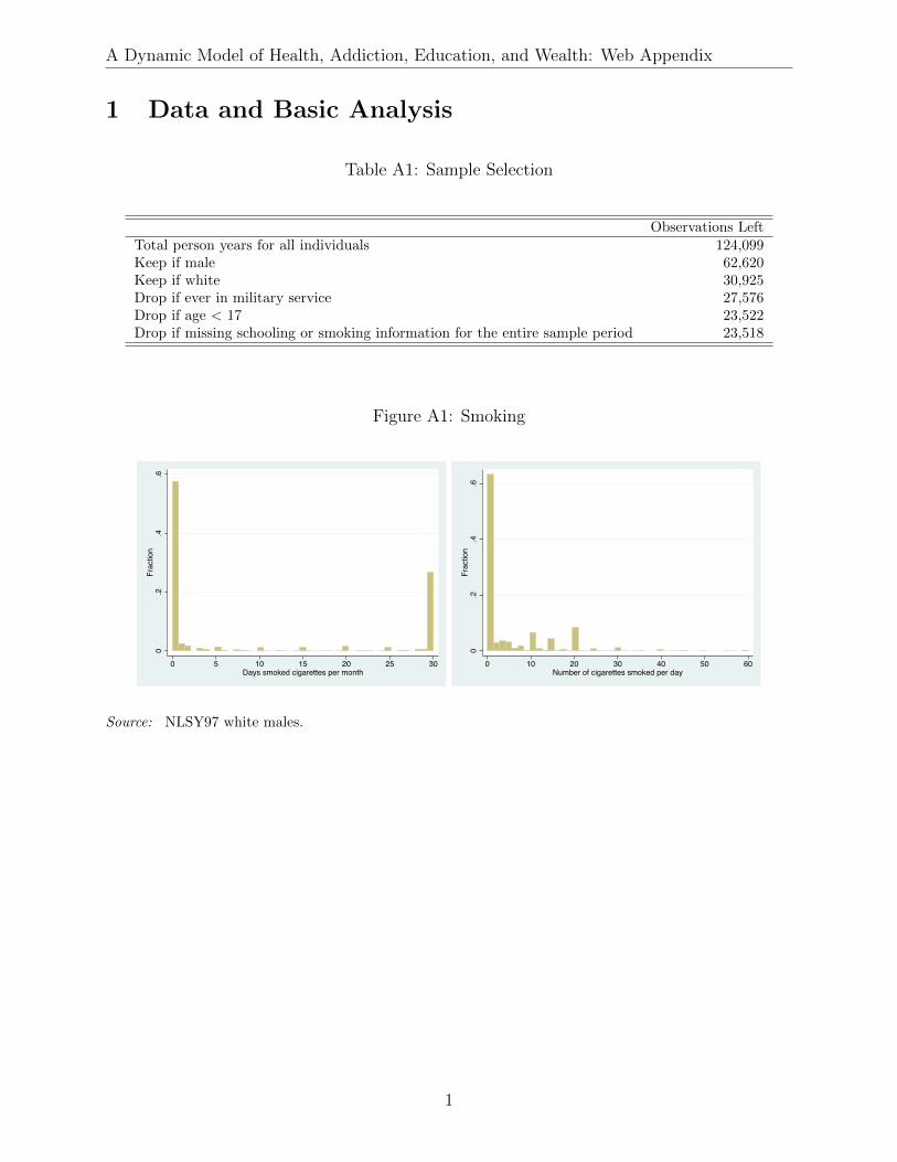
A Dynamic Model of Health, Addiction, Education, and Wealth: Web Appendix
1 Data and Basic Analysis
Table A1: Sample Selection
Observations LeftTotal person years for all individuals 124,099Keep if male 62,620Keep if white 30,925Drop if ever in military service 27,576Drop if age < 17 23,522Drop if missing schooling or smoking information for the entire sample period 23,518
Figure A1: Smoking
0.2
.4.6
Frac
tion
0 5 10 15 20 25 30Days smoked cigarettes per month
0.2
.4.6
Frac
tion
0 10 20 30 40 50 60Number of cigarettes smoked per day
Source: NLSY97 white males.
1

A Dynamic Model of Health, Addiction, Education, and Wealth: Web Appendix
Figure A2: Education Gradient in Various Health Behaviors
0.1
.2.3
.4.5
Prob
abilit
y
< 12 yrs 12 yrs 13 to 15 yrs >=16 yrsSchooling Categories
Regular Smoking Heavy DrinkingExercise < 30 mins/wk Do Not Typically Eat Fruit
Source: NLSY97 white males aged 25 to 30. We create a dummy variable for heavy drinking based oncommonly used measures, including the Center for Disease Control and Prevention (CDC) which definesheavy drinking as more than 2 drinks per day for men, and 1 drink per day for women. We modified this tobe an average of 3 drinks or more per day, or 90 drinks per month.
Table A2: Cross-Correlation Table
Variables Regular Smoking Heavy Drinking Exercise < Do Not Typically30 mins/wk Eat Fruit
Regular Smoking 1.000
Heavy Drinking 0.136 1.000(0.000)
Exercise < 30 mins/wk 0.107 0.003 1.000(0.000) (0.773)
Do Not Typically Eat Fruit 0.140 0.052 0.158 1.000(0.000) (0.000) (0.000)
2
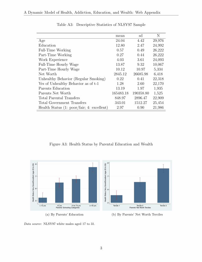
A Dynamic Model of Health, Addiction, Education, and Wealth: Web Appendix
Table A3: Descriptive Statistics of NLSY97 Sample
mean sd NAge 24.04 4.42 29,976Education 12.80 2.47 24,992Full-Time Working 0.57 0.49 26,222Part-Time Working 0.27 0.44 26,222Work Experience 4.03 3.61 24,093Full-Time Hourly Wage 13.87 9.32 10,067Part-Time Hourly Wage 10.12 10.97 5,334Net Worth 2845.12 26685.98 6,418Unhealthy Behavior (Regular Smoking) 0.22 0.41 22,318Yrs of Unhealthy Behavior as of t-1 1.28 2.60 22,170Parents Education 13.19 1.97 1,935Parents Net Worth 165483.18 190358.80 1,525Total Parental Transfers 848.97 2896.47 22,909Total Government Transfers 343.01 1512.27 25,454Health Status (1: poor/fair; 4: excellent) 2.97 0.90 21,986
Figure A3: Health Status by Parental Education and Wealth
.5
.6
.7
.8
Hea
lth S
tatu
s Ve
ry G
ood/
Exce
llent
(age
25
to 3
0)
< 12 yrs 12 yrs 13 to 15 yrs >=16 yrsParents' Schooling Categories
(a) By Parents’ Education
.5
.6
.7
.8
Hea
lth S
tatu
s Ve
ry G
ood/
Exce
llent
(age
25
to 3
0)
Tercile 1 Tercile 2 Tercile 3 Parents' Net Worth Terciles
(b) By Parents’ Net Worth Terciles
Data source: NLSY97 white males aged 17 to 31.
3

A Dynamic Model of Health, Addiction, Education, and Wealth: Web Appendix
Figure A4: Parental Education & Youth Education Outcomes
0.1
.2.3
.4.5
.6.7
.8.9
1 C
olle
ge A
ttend
ance
Rat
e
ASVAB AR Quartile 1 ASVAB AR Quartile 2 ASVAB AR Quartile 3 ASVAB AR Quartile 4
Parents' Schooling < 12 yrs Parents' Schooling = 12 yrs
Parents' Schooling 13 to 15 yrs Parents' Schooling >= 16 yrs
(a) College Attendance Rate at Age 21
0.1
.2.3
.4.5
.6.7
.8.9
1 4
-Yr C
olle
ge G
radu
atio
n R
ate
ASVAB AR Quartile 1 ASVAB AR Quartile 2 ASVAB AR Quartile 3 ASVAB AR Quartile 4
Parents' Schooling < 12 yrs Parents' Schooling = 12 yrs
Parents' Schooling 13 to 15 yrs Parents' Schooling >= 16 yrs
(b) 4-Year College Graduation Rate at Age 25
Figure A5: Parental Net Worth, & Youth Education Outcomes
0.1
.2.3
.4.5
.6.7
.8.9
1 C
olle
ge A
ttend
ance
Rat
e
ASVAB AR Quartile 1 ASVAB AR Quartile 2 ASVAB AR Quartile 3 ASVAB AR Quartile 4
Parents' Net Worth Tercile 1 Parents' Net Worth Tercile 2
Parents' Net Worth Tercile 3
(a) College Attendance Rate at Age 21
0.1
.2.3
.4.5
.6.7
.8.9
1 4
-Yr C
olle
ge G
radu
atio
n R
ate
ASVAB AR Quartile 1 ASVAB AR Quartile 2 ASVAB AR Quartile 3 ASVAB AR Quartile 4
Parents' Net Worth Tercile 1 Parents' Net Worth Tercile 2
Parents' Net Worth Tercile 3
(b) 4-Year College Graduation Rate at Age 25
4

A Dynamic Model of Health, Addiction, Education, and Wealth: Web Appendix
Figure A6: Parental Transfers By Parental Characteristics
050
01,
000
1,50
02,
000
2,50
0Pa
rent
al T
rans
fers
Parents' Net Worth T1 Parents' Net Worth T2 Parents' Net Worth T3
Parents' educ < 12 yrs Parents' educ = 12 yrs Parents' educ 13 to 15 yrs Parents' educ >= 16 yrs
(a) By Parents’ Net Worth & Education
050
01,
000
1,50
02,
000
Pare
ntal
Tra
nsfe
rs
17 18 19 20 21 22 23 24 25 26 27 28 29 30 31Age
(b) By Youth’s Age
Figure A7: Educational Gradient in Health, Smoking, Wages, and Wealth (Age 25 to 30)
.2
.43
.67
-.065-.045
.07
-.042
-.011
-.063
-.25-.31
-.45
3 3.3
6.7
5.5 4.7
17
.2.4
.6.8
0 -.1-.0
5.0
5.1
0
-.1-.0
5.0
50
-.5-.4
-.3-.2
0
24
68
0
510
1520
0
HighSchool
SomeCollege
4-YrCollege
HighSchool
SomeCollege
4-YrCollege
HighSchool
SomeCollege
4-YrCollege
Health Status BMI [18.5,30] Has Health Condition
Unhealthy Behavior Hourly Wage Net Worth (in Thousands)
5

A Dynamic Model of Health, Addiction, Education, and Wealth: Web Appendix
1.1 Regression Analysis
1.1.1 Unhealthy Behavior and Addiction
Let dq,t be an indicator variable of an individual engaging unhealthy behavior at age t. Weconsider a regression model of myopic unhealthy behavior as follows:
dq,t = β0 + β1dq,t−1 + β2
t−1∑τ=t0
dq,τ +X ′tγx + Z ′h,tγh + Z ′cγc + Z ′nγn + εq,t (1)
where∑t−1
τ=t0dq,τ is the accumulated years of past unhealthy behaviors from age t0 = 17 to
t−1, Xt is a vector of individual characteristics including education and age, Zh,t is a vectorof health measures at age t, and Zc and Zn are measures of the individual’s cognitive andnoncognitive skills, respectively.
Table A4 reports the regression results of Equation 1. As we can see, education is neg-atively correlated with unhealthy behavior and such correlation is statistically significant.Current unhealthy behavior is positively correlated with previous period’s unhealthy behav-ior and previously accumulated unhealthy behavior stock. Finally, individuals’ unhealthybehavior also correlates with various measures of health, and both the magnitude and signcan be different for different measures of health. This reduced-form regression analysisprovides a simple description of our data on regular smoking. It does not imply causalrelationship. It also does not take into account the rational anticipation effect of futureunhealthy behavior and health on current unhealthy behavior decision.
1.1.2 Adult Outcomes and Initial Health, Cognitive and Noncognitive Ability
Table A5 reports the OLS regression results of adult outcomes between age 25 to age 30 as afunction of individuals’ initial conditions. As we can see, measured initial health level has apositive and significant coefficient on individuals’ health, education, and wages. Measures ofcognitive ability are generally positively correlated with adult health, education, and wages.Early adverse behaviors are negatively correlated with adult health, education, and wealth,which suggests positive correlations between these adult outcomes and noncognitive ability,because noncognitive ability are measured by the absence of adverse behaviors. Parentaleducation and wealth also have a significant and positive correlation on individuals’ adultoutcomes.
6
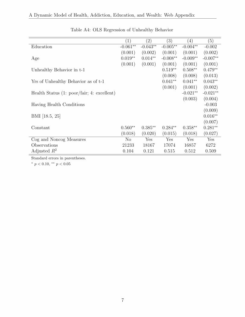
A Dynamic Model of Health, Addiction, Education, and Wealth: Web Appendix
Table A4: OLS Regression of Unhealthy Behavior
(1) (2) (3) (4) (5)Education -0.061∗∗ -0.043∗∗ -0.005∗∗ -0.004∗∗ -0.002
(0.001) (0.002) (0.001) (0.001) (0.002)Age 0.019∗∗ 0.014∗∗ -0.008∗∗ -0.009∗∗ -0.007∗∗
(0.001) (0.001) (0.001) (0.001) (0.001)Unhealthy Behavior in t-1 0.519∗∗ 0.508∗∗ 0.479∗∗
(0.008) (0.008) (0.013)Yrs of Unhealthy Behavior as of t-1 0.041∗∗ 0.041∗∗ 0.043∗∗
(0.001) (0.001) (0.002)Health Status (1: poor/fair; 4: excellent) -0.021∗∗ -0.021∗∗
(0.003) (0.004)Having Health Conditions -0.003
(0.009)BMI [18.5, 25] 0.016∗∗
(0.007)Constant 0.560∗∗ 0.385∗∗ 0.284∗∗ 0.358∗∗ 0.281∗∗
(0.018) (0.020) (0.015) (0.018) (0.027)Cog and Noncog Measures No Yes Yes Yes YesObservations 21233 18167 17074 16857 6272Adjusted R2 0.104 0.121 0.515 0.512 0.509
Standard errors in parentheses.∗ p < 0.10, ∗∗ p < 0.05
7
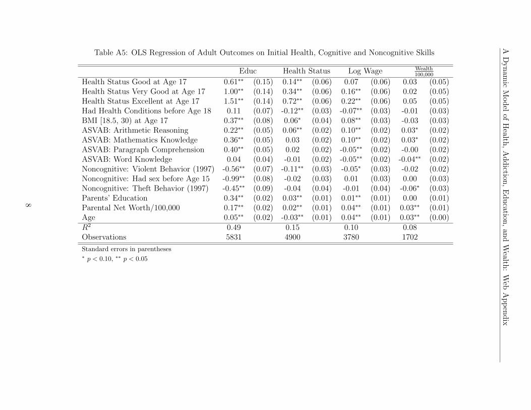
AD
ynam
icM
odel
ofH
ealth,
Addiction
,E
ducation
,an
dW
ealth:
Web
App
endix
Table A5: OLS Regression of Adult Outcomes on Initial Health, Cognitive and Noncognitive Skills
Educ Health Status Log Wage Wealth100,000
Health Status Good at Age 17 0.61∗∗ (0.15) 0.14∗∗ (0.06) 0.07 (0.06) 0.03 (0.05)Health Status Very Good at Age 17 1.00∗∗ (0.14) 0.34∗∗ (0.06) 0.16∗∗ (0.06) 0.02 (0.05)Health Status Excellent at Age 17 1.51∗∗ (0.14) 0.72∗∗ (0.06) 0.22∗∗ (0.06) 0.05 (0.05)Had Health Conditions before Age 18 0.11 (0.07) -0.12∗∗ (0.03) -0.07∗∗ (0.03) -0.01 (0.03)BMI [18.5, 30) at Age 17 0.37∗∗ (0.08) 0.06∗ (0.04) 0.08∗∗ (0.03) -0.03 (0.03)ASVAB: Arithmetic Reasoning 0.22∗∗ (0.05) 0.06∗∗ (0.02) 0.10∗∗ (0.02) 0.03∗ (0.02)ASVAB: Mathematics Knowledge 0.36∗∗ (0.05) 0.03 (0.02) 0.10∗∗ (0.02) 0.03∗ (0.02)ASVAB: Paragraph Comprehension 0.40∗∗ (0.05) 0.02 (0.02) -0.05∗∗ (0.02) -0.00 (0.02)ASVAB: Word Knowledge 0.04 (0.04) -0.01 (0.02) -0.05∗∗ (0.02) -0.04∗∗ (0.02)Noncognitive: Violent Behavior (1997) -0.56∗∗ (0.07) -0.11∗∗ (0.03) -0.05∗ (0.03) -0.02 (0.02)Noncognitive: Had sex before Age 15 -0.99∗∗ (0.08) -0.02 (0.03) 0.01 (0.03) 0.00 (0.03)Noncognitive: Theft Behavior (1997) -0.45∗∗ (0.09) -0.04 (0.04) -0.01 (0.04) -0.06∗ (0.03)Parents’ Education 0.34∗∗ (0.02) 0.03∗∗ (0.01) 0.01∗∗ (0.01) 0.00 (0.01)Parental Net Worth/100,000 0.17∗∗ (0.02) 0.02∗∗ (0.01) 0.04∗∗ (0.01) 0.03∗∗ (0.01)Age 0.05∗∗ (0.02) -0.03∗∗ (0.01) 0.04∗∗ (0.01) 0.03∗∗ (0.00)R2 0.49 0.15 0.10 0.08Observations 5831 4900 3780 1702
Standard errors in parentheses∗ p < 0.10, ∗∗ p < 0.05
8
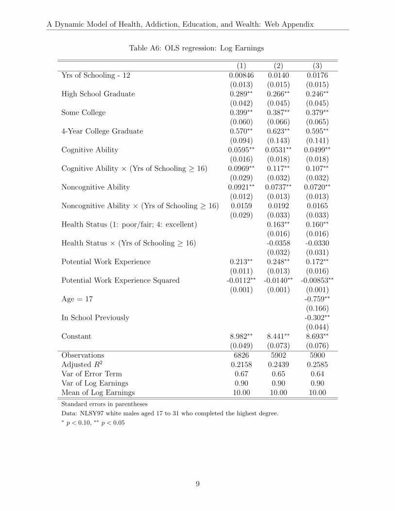
A Dynamic Model of Health, Addiction, Education, and Wealth: Web Appendix
Table A6: OLS regression: Log Earnings
(1) (2) (3)Yrs of Schooling - 12 0.00846 0.0140 0.0176
(0.013) (0.015) (0.015)High School Graduate 0.289∗∗ 0.266∗∗ 0.246∗∗
(0.042) (0.045) (0.045)Some College 0.399∗∗ 0.387∗∗ 0.379∗∗
(0.060) (0.066) (0.065)4-Year College Graduate 0.570∗∗ 0.623∗∗ 0.595∗∗
(0.094) (0.143) (0.141)Cognitive Ability 0.0595∗∗ 0.0531∗∗ 0.0499∗∗
(0.016) (0.018) (0.018)Cognitive Ability × (Yrs of Schooling ≥ 16) 0.0969∗∗ 0.117∗∗ 0.107∗∗
(0.029) (0.032) (0.032)Noncognitive Ability 0.0921∗∗ 0.0737∗∗ 0.0720∗∗
(0.012) (0.013) (0.013)Noncognitive Ability × (Yrs of Schooling ≥ 16) 0.0159 0.0192 0.0165
(0.029) (0.033) (0.033)Health Status (1: poor/fair; 4: excellent) 0.163∗∗ 0.160∗∗
(0.016) (0.016)Health Status × (Yrs of Schooling ≥ 16) -0.0358 -0.0330
(0.032) (0.031)Potential Work Experience 0.213∗∗ 0.248∗∗ 0.172∗∗
(0.011) (0.013) (0.016)Potential Work Experience Squared -0.0112∗∗ -0.0140∗∗ -0.00853∗∗
(0.001) (0.001) (0.001)Age = 17 -0.759∗∗
(0.166)In School Previously -0.302∗∗
(0.044)Constant 8.982∗∗ 8.441∗∗ 8.693∗∗
(0.049) (0.073) (0.076)Observations 6826 5902 5900Adjusted R2 0.2158 0.2439 0.2585Var of Error Term 0.67 0.65 0.64Var of Log Earnings 0.90 0.90 0.90Mean of Log Earnings 10.00 10.00 10.00
Standard errors in parentheses
Data: NLSY97 white males aged 17 to 31 who completed the highest degree.∗ p < 0.10, ∗∗ p < 0.05
9
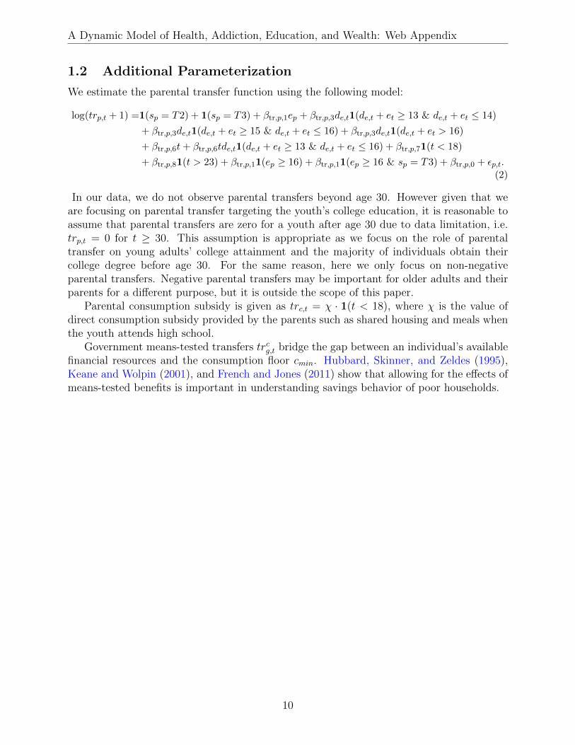
A Dynamic Model of Health, Addiction, Education, and Wealth: Web Appendix
1.2 Additional Parameterization
We estimate the parental transfer function using the following model:
log(trp,t + 1) =1(sp = T2) + 1(sp = T3) + βtr,p,1ep + βtr,p,3de,t1(de,t + et ≥ 13 & de,t + et ≤ 14)
+ βtr,p,3de,t1(de,t + et ≥ 15 & de,t + et ≤ 16) + βtr,p,3de,t1(de,t + et > 16)
+ βtr,p,6t+ βtr,p,6tde,t1(de,t + et ≥ 13 & de,t + et ≤ 16) + βtr,p,71(t < 18)
+ βtr,p,81(t > 23) + βtr,p,11(ep ≥ 16) + βtr,p,11(ep ≥ 16 & sp = T3) + βtr,p,0 + εp,t.(2)
In our data, we do not observe parental transfers beyond age 30. However given that weare focusing on parental transfer targeting the youth’s college education, it is reasonable toassume that parental transfers are zero for a youth after age 30 due to data limitation, i.e.trp,t = 0 for t ≥ 30. This assumption is appropriate as we focus on the role of parentaltransfer on young adults’ college attainment and the majority of individuals obtain theircollege degree before age 30. For the same reason, here we only focus on non-negativeparental transfers. Negative parental transfers may be important for older adults and theirparents for a different purpose, but it is outside the scope of this paper.
Parental consumption subsidy is given as trc,t = χ · 1(t < 18), where χ is the value ofdirect consumption subsidy provided by the parents such as shared housing and meals whenthe youth attends high school.
Government means-tested transfers trcg,t bridge the gap between an individual’s availablefinancial resources and the consumption floor cmin. Hubbard, Skinner, and Zeldes (1995),Keane and Wolpin (2001), and French and Jones (2011) show that allowing for the effects ofmeans-tested benefits is important in understanding savings behavior of poor households.
10

A Dynamic Model of Health, Addiction, Education, and Wealth: Web Appendix
Table A7: Estimation of Parental Transfer Functions
(1)Log (Parental Transfers + 1)
Parents’ Net Worth T2 0.247∗∗ (0.055)Parents’ Net Worth T3 0.540∗∗ (0.065)In First/Second Yr College 8.282∗∗ (0.673)In Third/Fourth Yr College 9.515∗∗ (0.738)In Graduate School 1.153∗∗ (0.146)Age -0.201∗∗ (0.013)Age * In College -0.306∗∗ (0.034)Age 17 -0.719∗∗ (0.096)> Age 23 -0.266∗∗ (0.091)Parents’ Schooling 12 years 0.134∗∗ (0.066)Parents’ Schooling 13 to 15 years 0.536∗∗ (0.066)Parents’ Schooling ≥ 16 years 1.306∗∗ (0.097)Parents’ Schooling ≥ 16 years * Parents’ Net Worth T3 0.096 (0.119)Constant 5.672∗∗ (0.274)Observations 16452Adjusted R2 0.255
Standard errors in parentheses
Parental transfers are in 2004 dollars.∗ p < 0.10, ∗∗ p < 0.05
11

A Dynamic Model of Health, Addiction, Education, and Wealth: Web Appendix
2 Parameter Estimates
Table B8: Parameter Estimates of Joint Initial Distribution of (θc, θc, log h17)
θc: Cognitive θn: Noncognitivelog h17: Log
Health
MeanParents Wealth 3rd Tercile 0.463 1.563 0.561
( 0.050 ) ( 0.093 ) ( 0.068 )Parents Wealth 2nd Tercile 0.050 1.522 0.140
( 0.050 ) ( 0.085 ) ( 0.065 )Parents 4-Yr College 0.609 1.156 0.114
( 0.069 ) ( 0.141 ) ( 0.090 )Parents Some College 0.377 0.652 0.094
( 0.043 ) ( 0.077 ) ( 0.062 )Parents High School 0.270 0.512 0.092
( 0.055 ) ( 0.107 ) ( 0.080 )Constant 0.347 0.390 0.273
(N.A.) (N.A.) (N.A.)
Variance Matrix
1.000(N.A.)
0.285 1.000( 0.050 ) (N.A.)
0.137 0.461 1.000( 0.039 ) ( 0.059 ) (N.A.)
Constant terms are normalized such thatEep,sp(µc(ep, sp)) = Eep,sp(µn(ep, sp)) = Eep,sp(µh(ep, sp)) = 0.
12
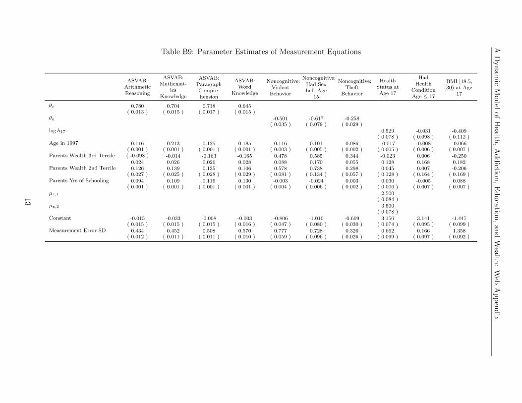
AD
ynam
icM
odel
ofH
ealth,
Addiction
,E
ducation
,an
dW
ealth:
Web
App
endix
Table B9: Parameter Estimates of Measurement Equations
ASVAB:ArithmeticReasoning
ASVAB:Mathemat-
icsKnowledge
ASVAB:ParagraphCompre-hension
ASVAB:Word
Knowledge
Noncognitive:ViolentBehavior
Noncognitive:Had Sexbef. Age
15
Noncognitive:Theft
Behavior
HealthStatus atAge 17
HadHealth
ConditionAge ≤ 17
BMI [18.5,30) at Age
17
θc 0.780 0.704 0.718 0.645( 0.013 ) ( 0.015 ) ( 0.017 ) ( 0.015 )
θn -0.501 -0.617 -0.258( 0.035 ) ( 0.079 ) ( 0.029 )
log h17 0.529 -0.031 -0.409( 0.078 ) ( 0.098 ) ( 0.112 )
Age in 1997 0.116 0.213 0.125 0.185 0.116 0.101 0.086 -0.017 -0.008 -0.066( 0.001 ) ( 0.001 ) ( 0.001 ) ( 0.001 ) ( 0.003 ) ( 0.005 ) ( 0.002 ) ( 0.005 ) ( 0.006 ) ( 0.007 )
Parents Wealth 3rd Tercile ( -0.098 ) -0.014 -0.163 -0.165 0.478 0.585 0.344 -0.023 0.006 -0.2500.024 0.026 0.026 0.028 0.088 0.170 0.055 0.128 0.168 0.182
Parents Wealth 2nd Tercile 0.126 0.139 0.135 0.106 0.578 0.738 0.298 0.045 0.007 -0.206( 0.027 ) ( 0.025 ) ( 0.028 ) ( 0.029 ) ( 0.081 ) ( 0.134 ) ( 0.057 ) ( 0.128 ) ( 0.164 ) ( 0.169 )
Parents Yrs of Schooling 0.094 0.109 0.116 0.130 -0.003 -0.024 0.003 0.030 -0.005 0.088( 0.001 ) ( 0.001 ) ( 0.001 ) ( 0.001 ) ( 0.004 ) ( 0.006 ) ( 0.002 ) ( 0.006 ) ( 0.007 ) ( 0.007 )
µz,1 2.500( 0.084 )
µz,2 3.500( 0.078 )
Constant -0.015 -0.033 -0.008 -0.003 -0.806 -1.010 -0.609 3.156 3.141 -1.447( 0.015 ) ( 0.015 ) ( 0.015 ) ( 0.016 ) ( 0.047 ) ( 0.080 ) ( 0.030 ) ( 0.074 ) ( 0.095 ) ( 0.099 )
Measurement Error SD 0.434 0.452 0.508 0.570 0.777 0.728 0.326 0.662 0.166 1.358( 0.012 ) ( 0.011 ) ( 0.011 ) ( 0.010 ) ( 0.059 ) ( 0.096 ) ( 0.026 ) ( 0.099 ) ( 0.097 ) ( 0.092 )
13

A Dynamic Model of Health, Addiction, Education, and Wealth: Web Appendix
Table B10: Parameter Estimates on Earnings Equation
Description Parameter Estimate S.E.Yrs of Schooling −12 βψ,e,0 0.0115 0.0029Yrs of Schooling ≥ 12, < 16 βψ,e,1 0.2102 0.0062Yrs of Schooling ≥ 16 βψ,e,3 0.3102 0.0045Cognitive Ability × Yrs of Schooling < 16 αψ,c 0.0372 0.0060Cognitive Ability × Yrs of Schooling ≥ 16 αψ,c 0.1581 0.0085Noncognitive Ability × Yrs of Schooling < 16 αψ,n 0.0779 0.0055Noncognitive Ability × Yrs of Schooling ≥ 16 αψ,n 0.0653 0.0061log (Health + 1) βψ,h 0.1833 0.0055Experience βψ,k 0.0862 0.0015Experience Squared/100 βψ,kk -0.2587 0.0041Part-Time While in School βw,p -0.6007 0.0074Age < 18 βψ,t -0.9436 0.1060Intercept βψ,0 7.8695 0.0112Shock Shape Parameter if Yrs of Schooling < 16 σw 0.7155 0.0110Shock Shape Parameter if Yrs of Schooling ≥ 16 σw 0.4912 0.0117Shock Boundary Parameter if Yrs of Schooling < 16 εw 9.4007 0.3948Shock Boundary Parameter if Yrs of Schooling ≥ 16 εw 26.5678 0.5459
Table B11: Parameter Estimates on Health Production Function: log(ht+1) − log(ht)
Description Parameter Estimate S.E.Intercept Constant βh,0 -0.0576 0.0058Log (Current Health) βh,h 0.0300 0.0043Log (Consumption/1000) βh,c 0.0011 0.0026Unhealthy Behavior βh,1 -0.0393 0.0083Years of Schooling-12 βh,e 0.0020 0.0023Cognitive Ability αh,c 0.0067 0.0036Noncognitive Ability αh,n 0.0067 0.0036S.D. of Health Shock σh 0.4000 0.0106
14
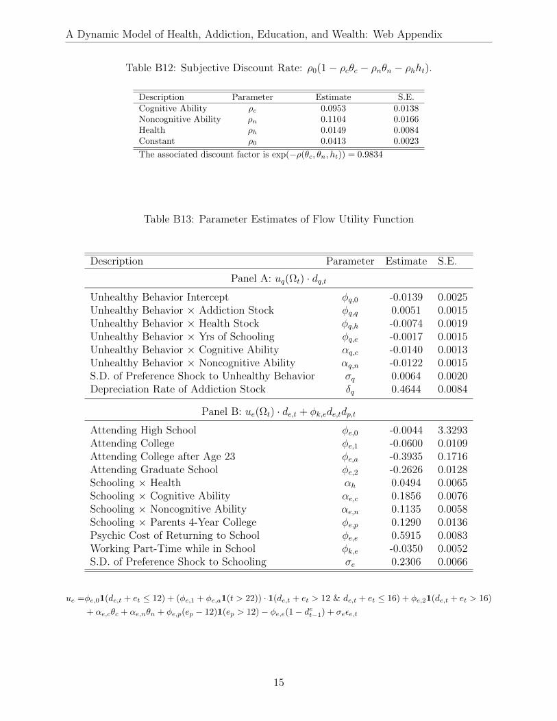
A Dynamic Model of Health, Addiction, Education, and Wealth: Web Appendix
Table B12: Subjective Discount Rate: ρ0(1 − ρcθc − ρnθn − ρhht).
Description Parameter Estimate S.E.Cognitive Ability ρc 0.0953 0.0138Noncognitive Ability ρn 0.1104 0.0166Health ρh 0.0149 0.0084Constant ρ0 0.0413 0.0023
The associated discount factor is exp(−ρ(θc, θn, ht)) = 0.9834
Table B13: Parameter Estimates of Flow Utility Function
Description Parameter Estimate S.E.
Panel A: uq(Ωt) · dq,tUnhealthy Behavior Intercept φq,0 -0.0139 0.0025Unhealthy Behavior × Addiction Stock φq,q 0.0051 0.0015Unhealthy Behavior × Health Stock φq,h -0.0074 0.0019Unhealthy Behavior × Yrs of Schooling φq,e -0.0017 0.0015Unhealthy Behavior × Cognitive Ability αq,c -0.0140 0.0013Unhealthy Behavior × Noncognitive Ability αq,n -0.0122 0.0015S.D. of Preference Shock to Unhealthy Behavior σq 0.0064 0.0020Depreciation Rate of Addiction Stock δq 0.4644 0.0084
Panel B: ue(Ωt) · de,t + φk,ede,tdp,t
Attending High School φe,0 -0.0044 3.3293Attending College φe,1 -0.0600 0.0109Attending College after Age 23 φe,a -0.3935 0.1716Attending Graduate School φe,2 -0.2626 0.0128Schooling × Health αh 0.0494 0.0065Schooling × Cognitive Ability αe,c 0.1856 0.0076Schooling × Noncognitive Ability αe,n 0.1135 0.0058Schooling × Parents 4-Year College φe,p 0.1290 0.0136Psychic Cost of Returning to School φe,e 0.5915 0.0083Working Part-Time while in School φk,e -0.0350 0.0052S.D. of Preference Shock to Schooling σe 0.2306 0.0066
ue =φe,01(de,t + et ≤ 12) + (φe,1 + φe,a1(t > 22)) · 1(de,t + et > 12 & de,t + et ≤ 16) + φe,21(de,t + et > 16)
+ αe,cθc + αe,nθn + φe,p(ep − 12)1(ep > 12) − φe,e(1 − det−1) + σeεe,t
15

A Dynamic Model of Health, Addiction, Education, and Wealth: Web Appendix
0.2
.4.6
.81
In S
choo
l 17 18 19 20 21 22 23 24 25 26 27
Age
99% CI NLSY Data Benchmark Model
(a) School Enrollment
0.1
.2.3
.4 U
nhea
lthy
Beh
avio
r
17 18 19 20 21 22 23 24 25 26 27 28 29 30 31 Age
99% CI NLSY Data Benchmark Model
(b) Unhealthy Behavior
810
1214
16 H
ighe
st G
rade
Com
plet
ed
< 12 yrs 12 yrs 13 to 15 yrs >=16 yrs Parents’ Schooling Categories
99% CI NLSY Data Benchmark Model
(c) Education By Parental Educa-tion
810
1214
16 H
ighe
st G
rade
Com
plet
ed
1 2 3 Parents’ Net Worth Terciles
99% CI NLSY Data Benchmark Model
(d) Education By Parental Wealth
Figure B8: Model Fit on School Enrollment and Unhealthy Behavior
References
French, Eric, and John Bailey Jones, 2011, The Effects of Health Insurance and Self-Insurance on Retirement Behavior, Econometrica 79, 693–732.
Hubbard, R. Glenn, Jonathan Skinner, and Stephen P. Zeldes, 1995, Precautionary Savingand Social Insurance, Journal of Political Economy 103, pp. 360–399.
Keane, Michael P., and Kenneth I. Wolpin, 2001, The Effect of Parental Transfers andBorrowing Constraints on Educational Attainment, International Economic Review 42,1051–1103.
16