A Dynamic Analysis of Skill Formation and NEET status Daniel Gladwell Gurleen Popli Aki Tsuchiya ISSN 1749-8368 SERPS no. 2015016 Originally Published: June 2015 Updated: October 2016

A Dynamic Analysis of Skill Formation and NEET status*

Daniel Gladwell a, Gurleen Popli b, Aki Tsuchiya c

October 2016

Abstract

This paper uses a dynamic Structural Equation Model to investigate the determinants of NEET (Not in

Education, Employment or Training) status in adolescents. We model: the cumulative formation of

cognitive ability over multiple periods through the life of the young person, up to completion of

compulsory education; and the impact that cognitive ability has on NEET status at one and two years

after compulsory education. Within this framework we address the issue of latent heterogeneity across

individuals. The analysis finds that cognitive ability remains the key predictor of NEET status, and

explains the persistence in NEET status. We also find evidence of significant indirect effects (of

magnitudes similar to direct effects of ability) of aspirations of the young person and their parents in the

prevention of NEET status. Health (general and mental) plays an important role in ability formation and

in explaining NEET status; however, its impact differs between the sexes.

JEL Classification: J21, I10, I21

Keywords: Adolescence, NEET, Dynamic modelling, Ability formation, Latent heterogeneity, LSYPE

a School of Health and Related Research, University of Sheffield, UK. (d.gladwell@shef.ac.uk)

b Department of Economics, University of Sheffield, UK. (g.popli@shef.ac.uk)

c School of Health and Related Research & Department of Economics, University of Sheffield, UK.

(a.tsuchiya@shef.ac.uk)

* An earlier version of the paper was circulated under the title of: ‘Estimating the impact of health on

NEET status.’ Sheffield Economics Research Paper Series, No. 2015016, University of Sheffield.

1

1. Introduction

NEET is a term used to refer to young people who are Not in Education, Employment or Training.

There are numerous choices available to young adults when their compulsory education ends. Some go

on to further education, others go into employment, and still others into training. There are, however, a

substantial number who do none of the above and are classified as NEETs: this would include all those

who are unemployed and looking for jobs, and those who are inactive (or discouraged workers). The

percentage of those who were classified as NEET in 2014 amongst 15-19 year olds in the UK was 9.5%;

international comparisons are complicated by the fact that compulsory school leaving age varies across

countries, but the average figure for OECD was 7.2% (OECD 2015).1

There are long term consequences of being NEET, both for the individual and society. For the

individuals evidence suggests that there is a degree of correlation between the status immediately after

compulsory education and a range of longer term outcomes. Those who leave full time education early

are unlikely to return to it (Dickerson and Jones 2004); and the resulting lower educational attainment is

associated with both lower pecuniary outcomes such as lifetime consumption and wealth (Card 1999 and

2001), and poorer non-pecuniary outcomes regarding adult health, marriage and parenting style

(Oreopoulos and Salvanes 2014). Further, youths who face spells of unemployment and inactivity

immediately after the end of their compulsory education demonstrate lower participation in the labour

market in the long term (Gregg 2001; Bell and Blanchflower 2011), and lower earnings later in life (Gregg

and Tominey 2005; Mroz and Savage 2006). There are associated societal costs: NEETs are more likely

to claim benefits and attach themselves to the informal economy; and loss of individual earnings results

in loss of tax revenues and increased welfare costs to the state (OECD 2013). In a UK based study Coles

et al. (2010) estimate the life-time costs of NEETs (16 to 18 years old) based on 2008 figures to be £12

billion: the sum is largely a result of accumulation of benefits and lost tax revenues, but also the (relatively

small) costs to the health and criminal justice systems.

1 The school leaving age in the UK is 16 (which is higher than the OECD median of 14 years), and almost

100% of the 15-16 year olds in the UK are in education.

2

The existing literature on the determinants of NEET generally takes the life of the young person

as one period, at the end of which we observe the outcome of interest, NEET status; the factors, current

and past, that impact NEET status are used as exogenous explanatory variables. From the empirical

literature (reviewed below) it is clear that one of the key variables that impact NEET status is the cognitive

ability (measured by educational achievement) of the young person. The literature so far has assumed

the cognitive ability of the young person as a given, and used it as an explanatory variable in the analysis

of NEET status. There exists a separate literature which looks at ability formation i.e. how ability evolves

over time (see for example Cunha and Heckman 2007).

Our paper makes two key contributions to the literature. The first contribution of the paper is

in modelling multiple periods through the life of the young person, building up over time to the outcome

of interest; we thus combine two strands of literature – we model both: the cumulative formation of

cognitive ability; and the impact this ability has on NEET status. We take into account that it is the

accumulation and interaction of different factors over time that determine cognitive ability at the different

stages of schooling, and NEET status following them.

The factors determining NEET status often discussed in the literature are: earlier academic

attainment of the young person; parental socioeconomic status; aspirations and attitudes, of the parents

and the young person; non-cognitive skills of the young person; and health of the young person. The

second contribution of this paper is in bringing all these determinants together within one framework.

In our analysis we model NEET as a dynamic concept; incorporating everything within a dynamic model

means we are able to look at the relative importance of the different determinants of NEET status and

the stage of a young person’s life when these factors have the biggest impact. We use a Structural

Equation Model (SEM) to understand the process that leads to the outcome of a young person being

NEET. The methodology allows us to address the issue of measurement error in estimating cognitive

ability and other latent factors. In addition, SEM allows the modelling of omitted variables as latent

(unobserved) heterogeneity.

We use the data from the Longitudinal Survey of Young People in England (LSYPE) which

followed a group of adolescents who completed compulsory education in 2008. The data has information

3

on: the educational progress and attainment of these young people throughout their secondary education

(starting age 11); their socioeconomic background; their own and their parents’ aspirations; their non-

cognitive skills; and their health. The final outcome we are interested in is being NEET at the end of

compulsory education (age 16) and persistence of this state a year-on at age 17/18. In our analysis we

pay particular attention to both the direct and the indirect (via past ability) impact of aspirations, non-

cognitive skills and health on the individuals’ likelihood of being NEET.

The remainder of this paper is organised as follows. In the next section, we briefly review the

relevant literature on the determinants of NEET status. Section 3 presents the empirical specification

that we use to estimate the dynamic model of ability formation and estimate the probability (and

persistence) of NEET status. Section 4 describes the data and the different variables we use in our

analysis. Section 5 presents our main results, and section 6 draws some conclusions.

2. The literature on the determinants of NEET status

Ryan (2001) carries out a cross national comparison of school-to-work transition (defined as the period

between the end of compulsory schooling and the attainment of full-time, stable employment). He looks

at seven countries: France, Germany, Japan, the Netherlands, Sweden, the UK and the US.

Socioeconomic disadvantage and low educational attainment remain the key driving forces for youth

inactivity and unemployment across all the seven countries, and this relationship is most acute in the UK

and the US. Continental Europe sees weaker correlations, which is attributed to successful vocational

education and apprenticeship programs (especially in Germany).

Crawford et al. (2011) use data from two different cohort studies in the UK (the LSYPE, and the

British Household Panel Survey (BHPS)) and the Labour Force Survey (LFS) to look at the choices made

by 16/17 and 17/18 year olds. Those who stay on in education after age 16 have the highest prior

educational attainments (KS2 and GCSE scores)2. While there does not seem to be a difference on

2 KS2 (Key Stage 2) exams are the national exams held at the end of primary school (age 11) in the UK;

and GCSE (General Certificate of Secondary Education) is awarded after the young people take the

national Key Stage 4 (KS4) exams at age 16.

4

average in the prior educational attainments of those who pursue jobs (with or without training) and

those who are NEET at 16/17, those who are still NEET two years on at age 18/19 had the lowest KS2

and GCSE scores. Their findings suggest that there is a degree of persistence in NEET status: 50% of

those who are NEET in the year immediately after the end of the compulsory education are NEET a

year on.3 For a given level of prior achievement, those who come from socioeconomically advantaged

families are the least likely to be NEETs at age 16/17.

Duckworth and Schoon (2012) use data from two UK cohort studies (the LSYPE and the British

Cohort Study (BCS)) and consider the ‘protective factors’ that result in some young people ‘beating the

odds’ i.e. avoiding NEET status despite unfavourable backgrounds. Their results show that prior

attainment, educational aspirations4 and engagement with school can reduce the cumulative risk faced by

a young person with multiple risk factors (low parental socioeconomic status, lone parents, social housing

and workless households). Yates et al. (2011) use the BCS data to discuss the role of aspirations in

determining NEET status. Key findings from their work suggest that 16-year olds who have uncertain

or misaligned aspirations5 are more likely to become NEET, especially young men from a low

socioeconomic background.

Other than educational attainments (often used as a measure of cognitive ability) there is now an

increasing recognition that personality traits (often used to capture non-cognitive skills) also matter for

education and labour market success; in particular, there is increasing stress on emotional stability, self-

3 For the LSYPE cohort specifically authors find that 40% of those who are NEET in the year

immediately after the end of the compulsory education are NEET a year on.

4 In both the LSYPE and the BCS, educational aspirations are represented by a question asked at age 14,

to both the young person and their parents, on whether or not the young person would like to continue

in post-compulsory education. 5 At age 16 the young people were asked about what they would like to do with their lives, where they

could choose from a list of jobs/careers/professions varying in the degree of training and qualifications

required. One of the responses that the young person could give was ‘can’t decide’ and all those who

choose this option (about 7% of the sample) are classified by the authors as having ‘uncertain aspirations’.

If the choice of the young person did not match their academic expectations then they were classified as

having ‘misaligned aspirations’ (Yates et al., 2011).

5

esteem and locus of control. Almlund et al. (2011) provide a review of studies looking at the link between

personality traits and economic outcomes; one of the findings they highlight in their review is that

personality traits are not fixed and can be altered by experience and investment, especially among the

young. Mendolia and Walker (2014) use data from the LSYPE to investigate the relationship between

personality traits and the likelihood of being NEET. The personality traits they consider include the

individual’s ability to persevere with long term goals (grit) and the extent to which an individual believes

that they can affect and control events (locus of control). Authors use propensity score matching, to

control for a set of adolescent and family characteristics, and find a significant relationship between these

traits and the probability of an individual being NEET.

There is a large literature looking at the relationship between health and educational outcomes

(Perri 1984; Currie and Hyson 1999). While these studies do not address NEET status as an outcome,

given that prior (academic) ability is a predictor of NEET status and health has an impact on the

acquisition of these abilities, health can be expected to have an indirect impact on NEET status.

Ding et al. (2009) use data from the Georgetown Adolescent Tobacco Research study to identify

the impact of Attention Deficit Hyperactivity Disorder, depression and obesity on Grade Point Average

(GPA) scores at high school. They find all three health conditions are significantly correlated with lower

test scores for both girls and boys; the results are robust to the inclusion of information on parents. The

negative impact of health problems and educational outcomes is supported by research undertaken by

Rees and Sabia (2009); the study uses data from the American National Longitudinal Study of Adolescent

Health (Add Health) to estimate the relationship between migraine headaches and educational outcomes

including GPA scores. The study finds migraines have a significant negative impact on the scores.

Studies have identified an increase in the prevalence of mental health difficulties amongst

adolescents (Collishaw et al. 2004; West and Sweeting 2003). The relationship between mental health

and educational attainment is bi-directional, where mental illness can potentially lead to poorer

educational attainment; and poor educational attainment can potentially increase the likelihood of mental

illness (Roeser et al. 19998). In an attempt to address this endogeneity Fletcher (2008) looks at the link

between depression in adolescence and later educational outcomes, using the Add Health data.

6

Controlling for past educational attainment and socioeconomic variables (parental education, income,

ethnicity, etc.), they find a negative association between earlier depression and later educational outcomes

only for females.

One recent study that looks at the direct impact of mental health on NEET status is Cornaglia et

al. (2015). They use the LSYPE and, controlling for past achievements, socioeconomic status of families,

and aspirations of both the young person and their parents, find a negative association between past

incidence of depression and educational outcomes, as measured by GCSE; and a positive association

between past incidence of depression and probability of being NEET. The results are stronger for girls.

In our paper we bring within one framework the different determinants of NEET status:

academic attainment, family socioeconomic status, aspirations, non-cognitive skills, and health of the

young person. We model both the cumulative formation of cognitive ability over the multiple periods

through the life of the young person, building up over time to the outcome of interest; and the impact

that this ability has on NEET status. The next section outlines our empirical strategy.

3. Estimation Method

To understand the dynamics of cognitive ability formation up to the end of compulsory education we

use the value added model of ability formation (Todd and Wolpin 2007), whereby an adolescent’s current ability

is a function of their prior ability and a host of exogenous variables which impact on the acquisition of

ability.6 Further, like Cunha and Heckman (2007) we assume the ability of the young person to be latent.

At the end of compulsory education, the stock of cognitive ability is then used to explain the young

person’s post-compulsory-education outcomes, in our case NEET status, and its persistence at the

following year.

For the analysis, we treat the period from birth to the end of primary school (ages 0 to 10/11

years) as 𝑡 = 0, setting the initial conditions. In particular, baseline latent cognitive ability (𝜃0) is

6 This framework allows for self-productivity skills; where self-productivity exists when higher ability at

time 𝑡 − 1 is associated with higher ability at time 𝑡 (Heckman and Masterov 2007).

7

measured by KS2 results at age 11. The young person’s life from age 11/12 to 17/18 is then divided into

four time periods (of uneven duration): 𝑡 = 1, … , 𝑇, with 𝑇 = 4. During years of compulsory

education, there are measures of cognitive ability at the end of each period: KS3 results at the end of

𝑡 = 1 when the child is 13/14 years old; and KS4-GCSE results at the end of 𝑡 = 2 when they are

15/16 years olds. Time periods 𝑡 = 3 and 4 cover post-compulsory education (16 to 17/18 years): for

these periods the outcome of interest is NEET status, in the academic year immediately after the end of

compulsory education (𝑡 = 3); and in the subsequent year (𝑡 = 4). NEET status is directly observable.7

We estimate the model using SEM which has two components: a structural model for the

dynamic pathway of interest from cognitive ability to NEET status; and a measurement model to estimate

the latent factors (Cunha et al. 2010; Popli et al. 2013).

3.1. Structural model

Let 𝜃𝑡 be the stock of latent cognitive ability (skill) of the child at time 𝑡. 𝜃𝑡 , depends on: past ability,

𝜃𝑡−1, and a set of exogenous covariates 𝑋𝑡. The dynamics for the first two time periods are given as,

𝜃𝑡 = 𝛾1𝑡𝜃𝑡−1 + 𝛾2𝑡 𝑋𝑡 + 𝜂𝑡 for 𝑡 = 1, and 2 (1)

where 𝛾1𝑡 and 𝛾2𝑡 are vectors of time-varying parameters to be estimated; and 𝜂𝑡 is the error term, such

that 𝐸(𝜂𝑡) = 0 and 𝐸(𝜂𝑡2) = 𝜎𝜂𝑡

2 .

For 𝑡 = 3 and 𝑡 = 4 the outcome of interest is NEET status at time 𝑡; the dynamics for 𝑡 = 3

and t = 4 are given as:

𝑌𝑡∗ = 𝛽1𝑡𝑌𝑡−1

∗ + 𝛽2𝑡𝜃𝑡−1 + 𝛽3𝑡 𝑋𝑡 + 𝜂𝑡 for 𝑡 = 3, and 4 (2)

where 𝑌𝑡∗ is the underlying unobserved variable that determines the NEET status; 𝛽1𝑡, 𝛽2𝑡, and 𝛽3𝑡 are

vectors of time-varying parameters to be estimated; and 𝜂𝑡 is the error term as above. For 𝑡 = 3, 𝑌𝑡∗

7 The approach we take to modelling NEET is similar to the approach, suggested by Cameron and

Heckman (1998), used in modelling schooling attainment as a stochastic process, where, instead of

modelling highest grade completed (or college entry), one divides schooling into stages and looks at a

sequence of grade transition probabilities to generate the probability of schooling attainment.

8

depends on past ability, 𝜃𝑡−1, and exogenous covariates 𝑋𝑡; 𝛽13 = 0, as there is no observation for

NEET status before 𝑡 = 3. Thus for 𝑡 = 3, we have:

𝑌3∗ = 𝛽23𝜃2 + 𝛽33 𝑋3 + 𝜂3 (2a)

For 𝑡 = 4, 𝑌𝑡∗ depends on 𝑌𝑡−1

∗ ; past ability, 𝜃𝑡−1; and some exogenous covariates 𝑋𝑡. In our

empirical application, the LSYPE does not have any measures for latent ability at 𝑡 = 3, 𝜃3. We therefore

make an assumption that the latent ability does not change significantly between 𝑡 = 3 and 𝑡 = 4, and

that 𝜃2 can be used as a good proxy for 𝜃3. This means that instead of 𝑌4∗ as a function of 𝜃3, we have

𝑌4∗ as a function of 𝜃2. Thus for 𝑡 = 4, we have:

𝑌4∗ = 𝛽14𝑌3

∗ + 𝛽24𝜃2 + 𝛽34 𝑋4 + 𝜂4 (2b)

Covariates in vector 𝑋𝑡 vary over time; we allow for the covariates to be both latent and observed

(we discuss the covariates in detail in section 4 below). A diagrammatic representation of the structural

model is given by a path diagram (Figure 1). The single headed arrows in the path diagram represent the

hypothesised direct effect of one variable on another. For example, the arrow from ability in period 1

(𝜃1) to ability in period 2 (𝜃2) indicates that we expect 𝜃1 to impact upon 𝜃2.

3.2. Measurement Model

Cognitive ability is assumed to be latent in our framework, so while we cannot observe ability the data

we use has a series of test scores which are correlated with the latent ability, and measure it with error.

We take into account this error in our measurement model:

𝑍𝑗,𝑡 = 𝜇𝑗,𝑡 + 𝛼𝑗,𝑡𝜃𝑡 + 𝜀𝑗,𝑡 𝑡 = 0, 1, 2 (3)

Where 𝑍𝑗,𝑡 for 𝑗 = 1, … , 𝑚𝑡 are the measures available for the latent variables at time 𝑡 (which may vary

across time). In order to enable identification, 𝑚𝑡 ≥ 3 is necessary. 𝛼𝑗,𝑡 are the factor loadings, which

can be interpreted as the amount of information that the measures (𝑍𝑗,𝑡) contain about the latent variable

(𝜃𝑡). 𝜇𝑗,𝑡 are the intercept; and 𝜀𝑗,𝑡 are the measurement errors, which capture the difference between

the observed measures and the unobserved latent variables.

9

For NEET status, we observe the discrete outcome, which we code as a binary variable. Random

utility theory models the observed outcome variable as:

𝑌𝑡 = 1 if 𝑌𝑡∗ > 𝑌𝐴

𝑌𝑡 = 0 otherwise

where 𝑌𝑡∗ can be interpreted as the utility from being NEET and 𝑌𝐴 is the utility from the alternative,

where the alternative can be any of the following: education (full time or part time), employment or

training. Without loss of generality we can assume 𝑌𝐴 = 0. The decision of the individual, in time period

𝑡 = 3, and 4 is modelled as:

𝑃(𝑌𝑡 = 1) = 𝑃 (𝑌𝑡∗ > 0| 𝛽1𝑡𝑌𝑡−1 + 𝛽2𝑡𝜃𝑡−1 + 𝛽3𝑡 𝑋𝑡)

= 𝑃 (𝜂𝑡 > −𝛽1𝑡𝑌𝑡−1 − 𝛽2𝑡𝜃𝑡−1 − 𝛽3𝑡 𝑋𝑡)

= 1 – 𝐹(−𝛽1𝑡𝑌𝑡−1 − 𝛽2𝑡𝜃𝑡−1 − 𝛽3𝑡 𝑋𝑡) 𝑡 = 3,4

(4)

where 𝐹(. ) is the cumulative distribution function for the error 𝜂𝑡 . We treat 𝜂𝑡 as a normal distribution,

and therefore estimate a probit model.

3.3. Structural model with latent heterogeneity

The structural model presented above is our baseline SEM. The baseline model assumes that all omitted

inputs are orthogonal to the included inputs. We next allow for time in-variant latent (unobserved)

heterogeneity (corresponding to fixed effects in panel data analyses) and estimate an alternative model,

given by equations (5) and (6) below:

𝜃𝑡 = 𝛾1𝑡𝜃𝑡−1 + 𝛾2𝑡 𝑋𝑡 + 𝜆 + 𝜂𝑡 for 𝑡 = 1, and 2 (5)

𝑌𝑡∗ = 𝛽1𝑡𝑌𝑡−1

∗ + 𝛽2𝑡𝜃𝑡−1 + 𝛽3𝑡 𝑋𝑡 + 𝜆 + 𝜂𝑡 for 𝑡 = 3, and 4 (6)

where 𝜆 is a scalar of all time in-invariant latent variables, representing individual heterogeneity, that

impact the dependent variables, 𝜃𝑡 and 𝑌𝑡∗. The specification given by equations (5) and (6), which

assumes linearity in parameters and time in-variance of 𝜆, is similar to the specification used by Cameron

and Heckman (1998) to model stochastic processes of school attainment.

10

3.4. Identification

To be able to identify all the parameters of interest in equations (1) to (4) we need to make the following

assumptions:

Assumption 1: 𝜂𝑡 is independent across individuals and over time, such that 𝐶𝑜𝑣(𝜂𝑡, 𝜂𝑠) = 0 for 𝑡 ≠ 𝑠.

Assumption 2: 𝜀𝑗,𝑡 has a mean of zero and is independent across individuals, over time for 𝑡 = 1, … 𝑇, and

across measures 𝑗 = 1, … , 𝑚𝑡 .

Assumption 3: 𝜀𝑗,𝑡 is independent of the latent variable 𝜃𝑡 , for 𝑡 = 1, … 𝑇, and 𝑗 = 1, … , 𝑚𝑡 .

Assumption 4: 𝜃0 is pre-determined and is allowed to be correlated with the time varying covariates in

vector 𝑋𝑡.

Assumption 4 is needed to estimate the model with a lagged dependent variable; if there is no

lagged dependent variable in the model we do not need this assumption.8 In addition, to be able to

estimate the model with latent heterogeneity, i.e. for identification of parameters of interest in equation

(3) to (6), we need following additional assumptions:

Assumption 5: There are no time in-variant covariates in vector 𝑋𝑡 .

Assumption 6: 𝜆 is correlated with 𝜃0, but is uncorrelated with 𝜂𝑡 and 𝜀𝑗,𝑡 for 𝑡 = 1, … 𝑇, and 𝑗 =

1, … , 𝑚𝑡.

Assumption 5 is similar to the one made for estimating fixed effect panel data models. This

assumption can be relaxed and we can include time in-variant variables in vector 𝑋𝑡 as long as we assume

that the time in-variant variables are uncorrelated with 𝜆; this is a hard to justify assumption as individual

heterogeneity is very likely to be correlated with the time in-variant variables (viz. gender and ethnicity).

Therefore, we do not adopt this approach and instead make assumption 5.9 This still allows for 𝜆 to be

correlated with the time varying variables in vector 𝑋𝑡 .

8 For a full specification of the variance-covariance matrix and the restrictions imposed on it to estimate

a model with a lagged dependent variable see Bollen and Brand (2010).

9 Removing the time in-variant variables will not result in omitted variable bias. Any independent impact

of time-invariant variables, like ethnicity and gender will be incorporated via the latent heterogeneity

11

Since the factor loadings in equation (3) can be identified only up to a scale it is necessary to

normalise them. We can either normalise the first factor loading, 𝛼1,𝑡 = 1, and allow the variance of

the latent variable to be freely estimated; or we can normalise the variance of the latent variable, 𝑉(𝜃𝑡) =

1, and let the factor loadings to be estimated freely; we do the latter. In addition, for the latent variables

we cannot separately identify both their mean, 𝐸(𝜃𝑡), and their intercept µ𝑗,𝑡. Therefore, we assume

𝐸(𝜃𝑡) = 0 and identify µ𝑗,𝑡.

For the empirical analysis, to aid computation, we further assume that 𝜂𝑡 and 𝜀𝑗,𝑡 have a normal

distribution, though this is not needed for identification.

3.5. Estimation and diagnostic statistics

One potential alternative to using SEM would be a panel model. However, SEM has a number of

advantages over panel data estimations (Bollen and Brand 2010): (1) unlike standard fixed or random

effect panel models, SEM allows the set of covariates at different time periods to vary, i.e. the covariates

can be specific to the stage of the young person’s life; (2) unlike panel models, SEM does not require the

coefficients of time-varying covariates included at different time periods to remain constant over time;

(3) unlike panel data models, SEM does not assume that error variances of equations are the same across

all time periods; and (4) unlike standard panel data analyses where estimation of models with lagged

dependent variables is often a problem, SEM estimates these with minimum assumptions.

There do exist estimation methods for the standard panel data model which overcome some of

these limitations. For example, to overcome limitation (2) we can interact the coefficients with time

dummies to allow covariates to have variable effects over time; similarly, for panel models with lagged

dependent variables Arellano-Bond estimation methods (Arellano and Bond 1991 and Arellano and

Bover 1995) can be used in the presence of appropriate instruments. See Baltagi (2013) for a full review

parameter. However, adopting this approach does have the disadvantage of precluding the identification

of their independent coefficients.

12

of panel models and solutions to a number of the limitations above. However, SEM allows us to address

all of these limitations within one framework.

One further advantage of estimating a dynamic SEM is that we can look at both the direct and

the indirect effects of one variable upon another. For example, coefficient 𝛽24 from equation (2b) gives

the estimate of the direct effect of ability at the end of compulsory education, 𝜃2, on NEET status in the

following year, 𝑌4. But we know that 𝜃2 also has an indirect impact on 𝑌4 via 𝑌3, given by 𝛽23 (equation

(2a)). The total effect of 𝜃2 on 𝑌4 is given by: 𝛽24 + 𝛽14 ∗ 𝛽23 (the direct effect + the indirect effect,

respectively). This involves the estimation of 𝛽14 ∗ 𝛽23 and its statistical significance; for details on this

estimation, see Muthen (2011).

Estimation is undertaken using the mean and variance adjusted weighted least squares (WLSMV)

estimator in MPlus v7.3 (Muthen and Muthen 2010). For the baseline model equations (1) to (4) are

estimated simultaneously; for the model allowing for latent heterogeneity equations (3) to (6) are

estimated simultaneously. The asymptotically distribution-free WLS was chosen instead of the maximum

likelihood (ML) approach because the ML approach requires the indicator variables used in equations (2)

to (4) to be continuous and multivariate normal. In our application many of these indicators are either

dichotomous or ordinal variables (see next section).

Since previous studies have indicated that the predictors of remaining in education can vary

between the genders (Fletcher 2008 and 2010), the models are estimated separately for females and males.

We use two diagnostic statistics to determine the goodness of model fit. Firstly, the Comparative

Fit Index (CFI) which accounts for the discrepancy between the data and the hypothesized model while

adjusting for sample size (Bentler 1990). Values from the CFI vary between 0 and 1 with higher values

indicating better model fit. Secondly, we use the root mean square error of approximation (RMSEA)

which shows the amount of variance that is not explained by the model. Values for the RMSEA again

vary between 0 and 1, where lower values are indicative of a better fitting model (Steiger and Lind 1980).

We take the guidance given by Hu and Bentler (1999) that for a model to be considered to fit the data

adequately it should have RMSEA < 0.06 and CFI > 0.90. In addition to using these diagnostic statistics

13

the validity of the model is judged on the basis of the individual parameter estimates produced.

Specifically, we consider whether they have face validity given expectations based on both wider

economic theory and the findings of previous empirical studies in this area.

4. Data and measurement

4.1 Overview of the dataset

The analysis is undertaken using data from the first five waves of the LSYPE. The study follows a cohort

of approximately 15,500 young people in English secondary schools. In the first wave, in 2004,

participants were aged 13/14. The survey was conducted annually, and by wave 5 the individuals were

aged 17/18. Until the LSYPE, the only nationally representative cohort studies undertaken in relatively

recent times were the BCS, which followed individuals born in 1970, and the Millennium Cohort Study

whose subjects are only now entering adolescence. The LSYPE is the first national survey for many years

to follow a group of English adolescents through much of their secondary education and into early

adulthood (Chowdry et al. 2009 and 2010)10. The main aim of the study was to provide evidence on the

factors central to individuals’ educational progress and attainment (Department for Education 2013).

For the first five waves the dataset contains responses from individual face to face interviews

with both the young person and their parents or guardians. We link the five waves of the LSYPE to the

four time periods and the initial conditions of our model (Figure 2 provides a visual representation of

how data from the different waves of the LSYPE are linked to the time periods). The information for

initial conditions and time period 1 of the analysis come from wave 1 of the LSYPE; information for

time period 2 comes from waves 2 and 3; time period 3 corresponds to wave 4; and time period 4

corresponds to wave 5. Additionally, for all children educated in the state sector the LSYPE is linked to

the National Pupil Database (NPD), an administrative database which contains information on national

10 The Avon Longitudinal Study of Parents and Children (University of Bristol 2013) contains the

responses of young people of a similar age. However, it does not contain respondents from the whole of

England; it only contains the responses of young people and their parents who live in Bristol and the

surrounding area.

14

examination results: KS2, KS3, KS4-GCSE (Department for Education 2011). We use these national

examination results as measures for cognitive ability.

While the longitudinal nature of the data allows for a dynamic analysis, this also imposes an

important limitation. Over the five waves of interviews a number of individuals drop out from the study.

It was only possible to include individuals from the LSYPE if they responded to a number of questions

across all five waves of data collection and if their examination results were available from the LSYPE-

NPD link11. This necessitated the exclusion of approximately two thirds of the original sample, leaving

us with 6,315 individuals (3,201 girls and 3,114 boys) for the analysis. Table 1 illustrates the effect of

attrition and non-response on the availability of individuals suitable for analysis. The LSYPE used a

stratified sampling approach; in our analysis we use robust standard errors clustered at the school level

and sampling weights from wave 5 (the final wave in our analysis). These weights take into account both

the sample design and non-response bias. See the report by Anders (2012) for further details.

4.2. Variables incorporated in the dynamic model

A list of all the variables along with detailed descriptions is provided in Appendix, Table A1. The

outcome variables and the covariates in each time period are shown in Figure 2, and discussed below.

Outcomes

Three measurement models for cognitive ability are estimated. Each attempts to model latent ability at

a different time period. The first model for baseline ability (𝜃0) incorporates indicators from the national

KS2 exams, which were undertaken when the individuals are aged 10/11, three years before being

interviewed for the LSYPE. The second measurement model for 𝜃1 is estimated using test scores from

11 We also drop our analysis all individuals who attended an independent school in wave 1. Not all

independent schools are linked to the NPD, as a result a substantial proportion of pupils from

independent schools do not have the national examination results in the LSYPE. There are 530

individuals who attended an independent school in wave 1; of these required examination results are

available for 86 individuals, but this increases the likelihood that these individuals are not representative

of the sub sample of individuals from independent schools. Therefore, we drop all 530 individuals.

15

the KS3 exams, taken when the individuals are aged 13/14 (LSYPE wave 1). The third measurement

model for 𝜃2 is estimated with indicators based on the test scores in KS4 (GCSEs), undertaken at the

end of compulsory education when the individuals are aged 15/16 (LSYPE wave 3).

From wave 4 of the LSYPE (when individuals are aged 16+) the respondents are no longer in

compulsory education. The LSYPE therefore contains data on the education or labour market status of

the young people: whether they are in full time education, in a job with training or without training, in

training, or NEET. A binary variable (𝑌𝑡) in wave 4 (𝑡 = 3) and wave 5 (𝑡 = 4) is created from this

information: the variable takes value 1 if the young person is NEET and 0 otherwise.

Covariates

The aspiration of the child is incorporated in the analysis by including their response to the question

“How likely do you think it is that you will ever apply to go to university to do a degree?”. Their responses

to this question when they are aged 14/15 (wave 2, 𝑡 = 2) and 15/16 (wave 3, 𝑡 = 2) are included in the

analysis. The aspiration variable of the child is coded 1 if the young person thinks it likely they will apply

to university and 0 otherwise.

Two variables relating to parental aspirations for the child are also included. In the first question

the parent (the primary carer) is asked what they think their child will do “when he/she reaches 16 and

can leave school”; in the second they are asked what they themselves would like their child to do when

they reach this same stage. The parent’s responses to these questions when their child is aged 14/15 and

15/16 are included in the analysis as predictions and preferences.12 The variables are coded 1 if the parent

indicates they think (or would like) their child to stay in education and 0 otherwise.

12 Within the literature on aspirations, there exists evidence that there is difference between predictions

and preferences, where the former is a more realistic assessment of the future outcomes and the latter

represents hopes and dreams (Jermin 2011).

16

Internal locus of control, a non-cognitive skill, was measured using the latent variable approach.13

The measurement model is populated using responses to three questions asked when aged 14/15 (LSYPE

wave 2). The young people were asked the extent to which they agreed with the statements: “I can pretty

much decide what will happen in my life”, “If someone is not a success in life, it is usually their own

fault”, “If you work hard at something you’ll usually succeed”. These questions have substantial

commonality with items used in Rotter’s (1966) seminal investigation into individuals’ perceived internal-

external control. To each of the questions individuals could respond “strongly agree” (coded as 4),

“agree”, “don’t know”, “disagree” or “strongly disagree” (coded as 0). Higher scores on the latent variable

are therefore associated with internal locus of control, the belief that events are contingent upon their

own behaviour. Conversely, lower scores are associated with external locus of control, the belief that

events are contingent upon either luck or the control of powerful others (Rotter 1966).

Mental health was measured using the latent variable approach in a manner similar to that adopted

for cognitive ability and locus of control. The 12-item General Health Questionnaire (GHQ-12)

(Goldberg and Williams 1988) was included in the survey when the individuals were aged 14/15 (LSYPE

wave 2) and also when they were aged 16/17 (LSYPE wave 4). In line with the study by Hankins (2008)

confirmatory factor analyses supported modelling mental health as a single latent variable while explicitly

accounting for measurement error that likely results from response bias on the negatively phrased items

of the GHQ-12. Additionally, confirmatory factor analyses supported the interpretation of the GHQ-

12 items as binary rather than likert variables. This interpretation of the items is consistent with the

findings of Goldberg et al. (1997). Following the findings of Hankins (2008), in the mental health

measurement models at each time period we allow for correlation in measurement error between the

negatively phrased items.

The variables available for capturing the difficulties in individuals’ general health vary across the

waves of the survey. There are three questions asked when the individuals are aged 13/14 (wave 1, 𝑡 =

13 LSYPE does not have information on the ‘Big Five’ personality traits (Almlund et al 2011) often

associated with non-cognitive skills.

17

1). In the first question the young person’s parent is asked whether their child has “any long-standing

illness, disability or infirmity”. The second and third questions are only asked if the parent responds yes

to the first. The second question asks if the problem makes it harder for their child “to attend school or

college regularly”; the third asks if the problem affects their child’s ability to “do his/her school work”.

The responses to these three questions are used to create two dummy variables (base in both is no health

problem): the young person has health problem not affecting school work or attendance; and the young

person has health problem that affects school work or attendance. In year 11 (wave 3, 𝑡 = 2) the

individuals were asked “In the last 12 months would you say your health has been very good, fairly good,

not very good or not good at all?”. In the analysis these responses are coded zero (for the responses

“very good” or “fairly good”) or 1 (for the responses “not very good” or “not good at all”). Finally, in

the first year post-compulsory education (wave 4) the initial screening question in wave 1 is asked to the

young person, the young person’s health is coded as 1 if they report a long-standing illness, disability or

infirmity and 0 otherwise.

Variables relating to household socioeconomic status14 are included from when the young people

are aged 13/14 (wave 1, 𝑡 = 1), 15/16 (wave 3, 𝑡 = 2), 16/17 (wave 4, 𝑡 = 3) and 17/18 (wave 5, 𝑡 =

4). These variables are based on the National Statistics socio-economic classification (NS-SEC) of the

household reference person. The household reference person is the person who owns or rents the

property the young person lives in. If the property is jointly owned or rented then it is the parent with

the highest income (Department for Education 2013). In the wave of interviews undertaken the second

year after compulsory education (wave 5) the household reference person is not explicitly listed.

14 Ideally we would have liked to use household income. However, household income is a variable with

particularly high number of missing observations, and if this variable were included in the analysis only

2,853 individuals would be available for inclusion. In order to avoid omitting such a high proportion of

individuals alternative variables which are highly correlated with household income, namely parental

education levels and family socioeconomic occupational class, are incorporated into the analysis as

controls.

18

Therefore, the variable identifying the household socioeconomic status of the family in this period takes

the value of the worker in the household with the highest occupational classification.

Where variables are incorporated in the structural model across multiple time periods, we take

the general approach to include the control variable that is from the period contemporaneous to the

outcome variable. This general approach is altered for the control variables relating to the child’s mental

health, aspirations of the child and parent, and the locus of control. Arguably these variables at time 𝑡

could be affected by the young person’s outcome of interest: test results or their education-labour market

choice at time 𝑡. In order to reduce the risk of reverse causality these control variables are taken from

the time period prior to the outcome variable.

Other control variables incorporated into the analysis include: the child’s birthweight; the month

of year the child was born; the child’s ethnicity; the mother’s education15; and the parental rating of the

child’s school and of the teachers. Apart from the young person’s ethnicity these variables are only

included as initial conditions. Ethnicity is included again in the regression which explores the predictors

of NEET status in the first year after compulsory education. This is because ethnicity may have an

independent effect on their choice over the education-labour market if racial discrimination is present

within the labour market, or perceived to be so by the young person. Data on the local area deprivation

first becomes available in 𝑡 = 2 (wave 2). The local index of multiple deprivation is therefore included

in the regression exploring the predictors of ability in the second time period.

4.3. Descriptive statistics

Table 2 presents the weighted summary statistics for the sample. There appears to be a large degree of

similarity between the sample of girls and boys with respect to control variables such as household

15 In order to reduce missingness single imputation was undertaken for missing responses for the variables

relating to mother’s education and the young person’s ethnicity. For example, though mother’s education

was generally taken from wave 1 if this was missing and it was reported in wave 2 the wave 2 value was

used; however, imputation was not undertaken for mother’s education if the mother confirmed she had

gained a qualification since wave 1.

19

socioeconomic status (with approximately 40% of the young people coming from the highest category –

managerial/professional – in wave 1); mother’s highest qualification (almost 40% of the mothers have

A-levels or above qualification); the parent’s rating of the child’s school and teachers (with almost 90%

of the parents rating the school as good or very good); and about 88% of the sample is white.

As a group, however, the girls’ mean points in their GCSE exams are higher than the boys’ in the

sample; similarly a larger proportion of girls achieve C or higher in their GCSE English exam. There is

a difference in the aspirations of the parents as well across genders. In wave 2 (age 14/15) 87% of the

parents of girls would like their daughters to stay in education after age 16, and 82% think that their

daughters will stay in education; the corresponding numbers for boys are 72% and 64%. By wave 3 (age

15/16) there is an upward revision in aspirations of the parents where 87% (72%) of parents for girls

(boys) think that the young person will stay on in education. There is an aspiration gap between girls and

boys themselves, with 67% of the girls in wave 3 thinking they are fairly likely or very likely to apply to

university; the corresponding number for boys is 53%.

At the end of compulsory education, 6% of the girls and 8% of the boys in our sample are

NEETs. A year later this number increases to 7% for girls and 11% for boys. Both the incidence of

NEET status and the persistence of NEET status is higher among boys; with 27% (33%) of the girls

(boys) who were NEET in wave 4 still NEET in wave 5.

5. Results

5.1. Dynamic SEM

Baseline Model

We first present the results (Table 3) from our base case model – the dynamic SEM which does not

account for latent heterogeneity.16 Starting from the results relating to ability formation in periods 𝑡 = 1

and 𝑡 = 2, past ability is significant in both equations; a one standard deviation (SD) increase in 𝜃0 leads

16 Factor loadings from the measurement models for the latent variables are not reported but are available

upon request.

20

to an increase of 0.84 SD in 𝜃1 (for both girls and boys), and similarly a one SD increase in 𝜃1 leads to

an increase of 0.79 SD in 𝜃2. We therefore have evidence supporting the “self-productivity” of skills.

For both girls and boys the higher prior aspirations of the young person and the predictions of their

parent (𝑡 = 2) have a positive impact on ability, while parental preferences have no significant impact

on ability. Similarly internal locus of control, a non-cognitive skill (𝑡 = 2), is associated with higher

ability supporting “cross-productivity” between non-cognitive and cognitive skills (Cuhna et al. 2010).

Health problems that affects schooling (𝑡 = 1) and poor self-reported health (𝑡 = 2) have a

significant negative impact on ability in the contemporaneous time period. For girls past mental health

difficulties have a negative impact on ability (𝑡 = 2); for boys, consistent with the literature, past mental

health is not significantly correlated with ability. Lower socioeconomic status (𝑡 = 1, 2) and a deprived

neighbourhood (𝑡 = 2) also appear to have a negative impact on ability formation. Belonging to an

ethnic minority has a significant negative impact on skill accumulation for boys; the effect is largely

insignificant for girls.

For NEET status in the period immediately after compulsory education (𝑡 = 3), it can be seen

that prior ability has a negative impact on the probability of being NEET. Controlling for prior ability,

the prior aspiration of the young person and the parent’s prediction that their child will remain in

education (t = 2) further significantly reduces the probability of the young person being NEET in the

subsequent wave.

For both girls and boys NEET status in time period 4 (𝑡 = 4) is significantly correlated with

NEET status in period 3 (𝑡 = 3) indicating a degree of persistence. For girls, after controlling for NEET

status at age 16/17, past ability maintains a negative impact on NEET status at age 17/18, while for boys,

past ability is not a significant predictor of NEET status at age 17/18. For both girls and boys past

mental health difficulties predict NEET status significantly. For girls higher socioeconomic status

remains a significant predictor of not being NEET; the coefficient is not significant for boys.

21

The fit diagnostic statistics indicate that the SEMs fit the data from both genders adequately; CFI

is well above the recommended level of 0.90 and RMSEA is below 0.05, as recommended. Additionally,

the individual parameter estimates reported appear to have face validity.

Model with latent heterogeneity

We turn to considering the potential impact of latent heterogeneity on the results. To estimate this model

we drop all time-invariant variables from the model (Assumption 5 above): birthweight, month of birth,

mother’s education, ethnicity, and local index of multiple deprivation. Comparing the results reported in

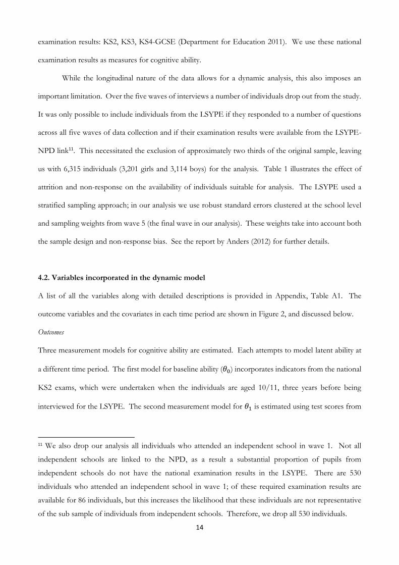
Table 3 (baseline model) and Table 4 (model with latent heterogeneity), controlling for latent

heterogeneity has a limited impact on the broad findings of the SEM; findings from the baseline model

are robust to inclusion of time-invariant latent heterogeneity. Past ability, aspirations of the young person

and that of their parents remain significant predictors of both ability and NEET status at age 16/17;

health problems impacting schooling have a significant negative impact on ability formation; and there

remains a significant persistence in NEET status over time, with past ability remaining a significant

predictor of NEET status at age 17/18. The fit diagnostic statistics indicate that the SEM fits the data

from both genders adequately; and the individual parameter estimates reported appear to have face

validity.

5.2. Indirect effects

Table 5 (age 16/17) and Table 6 (age 17/18) present the direct and indirect effects of a number of

variables on NEET status in time period 3 and 4, respectively, for the baseline model. While the indirect

effects of all the variables in the model on NEET status can be calculated we focus here only on the

indirect effects of ability, aspiration, locus of control and health on NEET status.

Given: i) the significant self-productivity of cognitive skills; ii) the significant impact of ability at

age 16 in reducing the risk of NEET status immediately after compulsory education at age 16/17; and

iii) significant persistence of NEET status over time: variables significantly associated with increased skill

accumulation in early adolescence commonly have a significant indirect effect on NEET status (both

22

immediately after compulsory education and in the subsequent year). For both girls and boys academic

ability in childhood and early adolescence are therefore significantly associated with a lower probability

of being NEET post compulsory education (Table 5) and in the following year (Table 6).

Similarly, the aspirations of the young person and their parent (when the young person is both

aged 14/15 and 15/16) and an orientation towards internal locus of control aged 14/15 is significantly

associated with a reduced risk of being NEET. A general health difficulty which affects schooling (aged

13/14) is also significantly associated with an increased risk of being NEET in both time periods. For

girls mental health difficulties aged 14/15 are significantly correlated with an increased risk of being

NEET in both time periods; for boys the correlation is not significant at traditional thresholds.

When controlling for latent heterogeneity, as with the direct effects reported in Table 4, the

estimated indirect effects (reported in Tables 7 and 8) are broadly similar to those estimated in the base

case model. Ability, aspiration and a general health difficulty which affects schooling are significantly

associated with an increased risk of being NEET. With respect to their indirect effect on future NEET

status the variables with the largest standardized coefficients are reported for: prior ability, prior

expectations of the young person and their parent, and an illness which affects the young person’s

schooling.

6. Concluding discussion

Ensuring young people start their adult lives in education, employment or training benefits both the

individuals concerned and society as a whole. The longitudinal nature of the data (LSYPE) and the SEM

approach used in this paper allow a dynamic analysis of the predictors of NEET status. To our

knowledge this is a first study which models multiple periods through the life of a young person

combining two strands of the literature (one on ability formation and another on the determinants of

NEET status), and puts together various determinants of NEET status within a single framework. We

also address the issue of measurement error in both ability and other factors of interest by using a latent

factor model, and model the omitted variables as latent (unobserved) heterogeneity. In contrast to

previous studies looking at the determinants of NEET status, the incorporation of a dynamic analysis

23

allows us not only to investigate the relative importance of the different determinants of NEET status,

but it additionally allows an analysis of the period in which these different determinants have their greatest

impact and the pathway through which their cumulative impact is realised.

Similar to the existing literature we find evidence of self-productivity in cognitive skill formation

and cross-productivity between cognitive and non-cognitive skills. Cogntive ability plays a substantial

role in protecting or exposing individuals to the risk of being NEET and explains the persistence in

NEET status.

Household SES is an important predictor of ability, for both girls and boys, where higher

household SES status (managerial/professional) predicts higher ability formation. While household SES

is not associated with NEET status a year after the end of compulsory schooling, for girls only it is

important in predicting the continuation of NEET status a year on, where girls from higher SES are less

likely to continue being NEET.

As suggested by the literature health problems that affect schooling has a direct negative impact

on ability formation early on (age 13/14). The indirect effect remains significant later on in life via

reduced ability formation. Later on (age 15/16) while for girls its poor mental health that impacts ability

negatively, for boys it is general health difficulties that are significant. Mental health continues to be

significant for explaining NEET status for girls and boys. However, when we allow for latent

heterogeneity mental health difficulties do not significantly predict either ability or NEET status for girls

or boys – this is contrary to the findings of Cornaglia et al. (2015).

Parental predictions and young person’s own university plans are important for later ability and

NEET, but parental preferences are not, so what seems to be important is not higher aspirations in

themselves, but realistic aspirations.

The paper’s findings have important policy implications. As noted there is a strong relationship

between both prior academic ability and future academic ability, and between prior academic ability and

future NEET status. Policy makers aiming to minimise the number of young people who start their

working life in unemployment may do well to consider how they can best help young people develop

their academic ability throughout adolescence. To some extent it could be argued that this process starts

24

even earlier, in the early childhood of the individual. Our analysis shows, however, that even when pre-

adolescent academic ability is controlled for, other influences on the individual’s further accumulation of

ability remain significant. These include factors such as their mother’s education, the parent-rated quality

of their school, the deprivation of their local area and their health problems. Interventions in early

childhood and late adolescence may both have a role, particularly in supporting those who come from

disadvantaged backgrounds and have health difficulties that affect their schooling. The research

presented supports the notion that while skill formation remains the key determinant of future NEET

status, individuals’ learning opportunities need to be protected and facilitated throughout their

adolescence if a society aims for all to be able to engage in its labour market.

Acknowledgements: We are grateful to the Department of Education for the use of the Longitudinal

Survey of Young People England (LSYPE), and to the UK Data Archive and Economic and Social Data

Service for making them available. Daniel Gladwell is funded by the University of Sheffield Faculty of

Medicine Dentistry and Health Scholarship. We would like to thank Mark Bryan, David Fairris, Steve

McIntosh, Imran Rasul, Jennifer Roberts; and participants at the Faculty of Social Sciences Research

Conference; Health Economists’ Study Group meeting June 2015; University of Sheffield, September

2015; and at the CLOSER conference, London, November 2015, for their helpful comments. All

responsibility for the analysis and interpretation of these data lies with the authors.

25

References

1. Almlund, M., Duckworth, A. L., Heckman, J. and Kautz, T. (2011). Personality Psychology and

Economics. In Handbook of the Economics of Education, vol. 4, ed. Hanushek E.A., Machin, S., and

Wessmann, L., 1-181.

2. Anders, J. (2012) Using the Longitudinal Study of Young People in England for research into Higher

Education access. Department of Quantitative Social Science Working Paper No . 12-13 December

2012 (No. 12-13). London.

3. Arellano, M. and Bond, S. (1991) Some Tests of Specification for Panel Data: Monte Carlo Evidence

and an Application to Employment Equations. The Review of Economic Studies, 58(2), 277-297.

4. Arellano, M. and Bover, O. (1995) Another Look at the Instrument Variable Estimation of Error-

Components Models. Journal of Econometrics, 8(1), 29-51.

5. Baltagi, B. (2013) Econometric Analysis of Panel Data. Wiley

6. Bentler, P. (1990) Comparative fit indexes in structural models. Psychological Bulletin, 107(2), 238–246.

7. Bell, D. and Blanchflower, D. (2011) Young people and the Great Recession. Oxford Review of

Economic Policy, 27(2), 241-267.

8. Bollen, K. and Brand, J. (2010) A general panel model with random and fixed effects: A structural

equations approach. Social Forces, 89(1), 1-34.

9. British Cohort Survey (BCS): http://www.cls.ioe.ac.uk

10. British Household Panel Survey (BHPS): https://www.iser.essex.ac.uk/bhps.

11. Cameron, S. and Heckman, J. (1998). Life cycle schooling and dynamic selection bias: Models and

evidence for five cohorts of American males. The Journal of Political Economy, 106(2), 262-333.

12. Card, D. (1999) The causal effect of education on earnings. In Handbook of Labor Economics, vol. 3A,

ed. Orley C. Ashenfelter and David Card, 1801-1863.

13. Card, D. (2001) Estimating the return to schooling: Progress on some persistent econometric

problems. Econometrica, 69(5), 1127-1160.

14. Chowdry, H., Crawford, C. and Goodman, A. (2009) Drivers and Barriers to Educational Success:

Evidence from the Longitudinal Study of Young. London.

15. Chowdry, H., Crawford, C and Goodman, A. (2010) The role of attitudes and behaviours in

explaining socio-economic differences in attainment at age 16 (No. 10, 15). London.

16. Coles, B., Godfrey, C., Keung, A., Parrot, S. and Bradshaw, J. (2010) Estimating the life-time cost of

NEET: 16-18 year olds not in Education, Employment or Training. Research conducted for the

Audit Commission, July 2010. http://php.york.ac.uk/inst/spru/pubs/ipp.php?id=1776

17. Collishaw, S., Maughan, B., Goodman, R. and Pickles, A. (2004) Time trends in adolescent mental

health. Journal of Child Psychology and Psychiatry, 45(8), 1350–1362.

18. Cornaglia, F., Crivellaro, E. and Mcnally, S. (2015) Mental Health and Education Decisions. Labour

Economics, 33, 1-12.

26

19. Crawford, C., Duckworth, K., Vignoles, A. and Wyness, G. (2011) Young people's education and

labour market choices aged 16/17 to 18/19. London: Department of Education.

20. Currie, J. and Hyson, R. (1999) Is the Impact of Health Shocks Cushioned by Socioeconomic Status?

The Case of Low Birthweight. American Economic Review, 89(2), 245-250.

21. Cunha, F. and Heckman, J. (2007) The technology of skill formation. American Economic Review, 97(2):

31-47.

22. Cunha, F., Heckman, J. and Schennach, S. (2010) Estimating the Technology of Cognitive and

Noncognitive Skill Formation. Econometrica, 78(3), 883–931.

23. Department for Education. (2011) LSYPE User Guide to the Datasets: Wave 1 to Wave 7 (pp. 1–

103). Retrieved from

http://www.esds.ac.uk/doc/5545/mrdoc/pdf/5545lsype_user_guide_wave_1_to_wave_7.pdf

24. Department for Education. (2013) About LSYPE. Retrieved from:

https://www.education.gov.uk/ilsype/workspaces/public/wiki/Welcome/LSYPE

25. Dickerson, A. and Jones, P. (2004) Estimating the Impact of a Minimum Wage on the Labour Market

Behaviour of 16 and 17 Year Olds.

26. Ding, W., Lehrer, S. F., Rosenquist, J. N. and Audrain-McGovern, J. (2009). The impact of poor

health on academic performance: New evidence using genetic markers. Journal of Health Economics,

28(3), 578-597.

27. Duckworth, K. and Schoon, I. (2012). Beating the Odds: Exploring the Impact of Social Risk on

Young People's School-to-Work Transitions during Recession in the UK. National Institute Economic

Review, 222(1), R38-R51.

28. Fletcher, J. (2008) Adolescent depression: diagnosis, treatment, and educational attainment. Health

Economics, 1235 (December 2007), 1215–1235.

29. Fletcher, J. (2010) Adolescent depression and educational attainment: results using sibling fixed

effects. Health Economics, 871 (July 2009), 855–871.

30. Goldberg, D. P., Gater, R., Sartorius, N., Ustun, T. B., Piccinelli, M., Gureje, O. and Rutter, C. (1997)

The validity of two versions of the GHQ in the WHO study of mental illness in general health care.

Psychological Medicine, 27(1), 191–7

31. Goldberg, D. P. and Williams, P. (1988) A user’s guide to the General Health Questionnaire. (D. P.

Goldberg & P. Williams, Eds.). Windsor: NFER-Nelson.

32. Gregg, P. (2001) The impact of youth unemployment on adult unemployment in the NCDS. The

Economic Journal, 111 (475), pp. 626-563.

33. Gregg, P. and Tominey, E. (2005) The wage scar from male youth unemployment. Labour Economics,

12(4), 487-509.

34. Hankins, M. (2008) The factor structure of the twelve item General Health Questionnaire (GHQ-

12): the result of negative phrasing? Clinical Practice and Epidemiology in Mental Health, 4(10), 1–8.

27

35. Heckman, J. and Masterov, D. V. (2007) The Productivity Argument for Investing in Young

Children. Review of Agricultural Economics, 29(3), 446–493.

36. Hu, L. and Bentler, P. M. (1999) Cutoff criteria for fit indexes in covariance structure analysis:

Conventional criteria versus new alternatives. Structural Equation Modeling: A Multidisciplinary Journal,

6(1), 1–55.

37. Jerrim, J. (2011). Disadvantaged children’s “low” educational expectations: Are the US and UK really

so different to other industrialized nations? (No. 11-04). Department of Quantitative Social Science-

UCL Institute of Education, University College London.

38. Labour Force Survey (LFS): The LFS Users Guide Volume 1: Background and Methodology’

(http://www.ons.gov.uk/ons/guide-method/method-quality/specific/labour-market/labour-

market-statistics/index.html)

39. Longitudinal Survey of Young People in England (LSYPE):

https://www.education.gov.uk/ilsype/workspaces/public/wiki/Welcome/LSYPE

40. Mendolia, S. and Walker, I. (2014). Do NEETs Need Grit? IZA Discussion Paper No. 8740.

41. Meschi, E., Swaffield, J. and Vignoles, A. (2011). The Relative Importance of Local Labour Market

Conditions and Pupil Attainment on Post-Compulsory Schooling Decisions. IZA Discussion Paper

No. 6143.

42. Millennium Cohort Study (MCS): http://www.cls.ioe.ac.uk/mcs

43. Mroz, T. and Savage, T. (2006). The long-term effects of youth unemployment. Journal of Human

Resources, 41(2), 259-293.

44. Muthén, L. and Muthén, B. (2010). Mplus User’s Guide, Sixth Edition. Los Angeles, CA: Muthén &

Muthén.

45. Muthén, B. (2011). Applications of causally defined direct and indirect effects in mediation analysis

using SEM in Mplus. Unpublished working paper, www. statmodel. com.

46. National Longitudinal Study of Adolescent Health (Add Health):

http://www.cpc.unc.edu/projects/addhealth

47. OECD (2015) Education at a Glance 2015: OECD Indicators (www.oecd.org/edu/eag.htm).

48. OECD (2013) Education at a Glance 2013: OECD Indicators

(www.oecd.org/edu/eag2013%20(eng)--FINAL%2020%20June%202013.pdf)

49. Oreopoulos, P. and Salvanes, K. (2011). Priceless: The nonpecuniary benefits of schooling. The

Journal of Economic Perspectives, 159-184.

50. Perri, T. (1984). Health status and schooling decisions of young men. Economics of Education Review,

3(3), 207-213.

51. Popli, G., Gladwell, D. and Tsuchiya, A. (2013) Estimating the critical and sensitive periods of

investment in early childhood: A methodological note. Social Science and Medicine, 97(C), pp. 316-324.

28

52. Rees, D. and Sabia, J. (2009). The Effect of Migraine Headache on Educational Attainment. The

Journal of Human Resources, 46(2), 317–332.

53. Roeser, R. Eccles, J. and Strobel, K. (1998). Linking the study of schooling and mental health:

Selected issues and empirical illustrations at the level of the individual. Educational Psychologist, 33(4),

153–176.

54. Rotter, J. (1966). Generalized expectancies for internal versus external control of reinforcement.

Psychological monographs: General and applied, 80(1), 1-28.

55. Ryan, P. (2001). The School-to-Work Transition: A Cross-National Perspective. Journal of Economic

Literature, 39(1), 34–92.

56. Steiger, J. and Lind, J. (1980). Statistically based tests for the number of common factors. Annual

Meeting of the Psychometric Society, Iowa City.

57. Todd, P. and Wolpin, K. (2007). The production of cognitive achievement in children: Home,

school, and racial test score gaps. Journal of Human Capital, 1(1), 91-136.

58. University of Bristol. (2013). Avon Longitudinal Study of Parents and Children. Retrieved from

http://www.bristol.ac.uk/alspac/participants/

59. West, P. and Sweeting, H. (2003). Fifteen, female and stressed: Changing patterns of psychological

distress over time. Journal of Child Psychology and Psychiatry and Allied Disciplines, 44, 399–411.

60. Yates, S., Harris, A., Sabates, R. and Staff, J. (2011). Early occupational aspirations and fractured

transitions: a study of entry into ‘NEET’status in the UK. Journal of Social Policy, 40(03), 513-534.

29

Table 1: Attrition and missing variables in the LSYPE

Wave

(year)

Age of YP Total Number of YP

Interviewed at each

Wave

Number of YP

Remaining from

Wave 1 – 5*

Number of YP at each

Wave with the

Required Data for

Inclusion+

1 (2004) 13/14 years 15,770 15,770 11,013

2 (2005) 14/15 years 13,539 13,539 9,539

3 (2006) 15/16 years 12,439 12,437 8,474

4 (2007) 16/17 years 11,801 11,425 7,372

5 (2008) 17/18 years 10,430 10,158 6,315

Notes:

*The number of young people (YP) interviewed in a given wave who were also present for all of the previous waves. + The number of young people present in a given wave and in each of the previous waves, with no missing data.

30

Table 2: Descriptive Statistics

Variable Girls (n=3201) Boys (n=3114)

mean S.D.* mean S.D.*

t = 0 (LSYE Wave 1)

KS2 Score: English 27.56 3.97 26.24 4.39

KS2 Score: Maths 26.75 4.63 27.24 4.88

KS2 Score: Science 28.57 3.53 28.76 3.52

Birth weight 3.25 0.57 3.41 0.60

Mother: A level or above 0.39 - 0.39 -

Mother: GCSE/lower qualification 0.44 - 0.44 -

Mother: has no qualification or no mother (base category) 0.18 - 0.17 -

Ethnicity: White (base category) 0.88 - 0.89 -

Ethnicity: Mixed 0.02 - 0.02 -

Ethnicity: Indian 0.02 - 0.03 -

Ethnicity: Pakistani/Bangladeshi 0.03 - 0.03 -

Ethnicity: Caribbean/African 0.02 - 0.02 -

Ethnicity: Other 0.02 - 0.01 -

School year month 6.28 3.44 6.28 3.49

t = 1 (LSYPE Wave 1)

KS3 Score: English 35.04 5.74 33.00 6.12

KS3 Score: Maths 36.51 7.50 36.80 7.84

KS3 Score: Science 34.20 6.33 34.14 6.54

Illness not affecting schooling 0.07 - 0.09 -

Illness affecting schooling 0.05 - 0.07 -

Parental rating of school 0.89 - 0.90 -

Parental rating of teachers 0.88 - 0.87 -

Household SES: Managerial/Professional 0.41 - 0.38 -

Household SES: Intermediate 0.19 - 0.22 -

Household SES: Routine/Manual 0.37 - 0.36 -

Household SES: Long term unemployed (base category) 0.03 - 0.03 -

t = 2 (LSYPE Wave 2)

University plans 0.67 - 0.56 -

Parent thinks YP will do 0.82 - 0.64 -

Parent would like YP to do 0.87 - 0.72 -

LC: Decide Happens 2.40 1.09 2.42 1.15

LC: Failure is their fault 2.26 1.13 2.48 1.13

LC: Work hard usually succeed 3.23 0.72 3.20 0.75

GHQ-12

Recently lost sleep 0.25 - 0.12 -

Recently under strain 0.33 - 0.20 -

Recent difficulties 0.25 - 0.14 -

Recently felt unhappy 0.31 - 0.14 -

Recently losing confidence 0.24 - 0.11 -

Recently felt worthless 0.16 - 0.07 -

Recently able to concentrate 0.18 - 0.10 -

Recently not useful 0.10 - 0.07 -

Recently made decisions 0.07 - 0.04 -

31

Variable Girls (n=3201) Boys (n=3114)

mean S.D.* mean S.D.*

Recently enjoyed activities 0.12 - 0.08 -

Recently faced up to problems 0.10 - 0.05 -

Recently felt happy 0.14 - 0.07 -

Local Index of Multiple Deprivation 21.17 16.01 21.47 16.04

t = 2 (LSYPE Wave 3)

GCSE Points 411.19 144.10 374.36 154.49

GCSE English 0.71 - 0.56 -

GCSE Maths 0.60 - 0.59 -

University plans 0.67 - 0.53 -

Parent thinks YP will do 0.87 - 0.72 -

Parent would like YP to do 0.89 - 0.74 -

Young person’s health 0.04 - 0.02 -

Household SES: Managerial/Professional 0.41 - 0.39 -

Household SES: Intermediate 0.14 - 0.14 -

Household SES: Routine/Manual 0.32 - 0.33 -

Household SES: Currently not working (base category) 0.13 - 0.14 -

t = 3 (LSYPE Wave 4)

NEET$ 0.06 - 0.08 -

GHQ-12

Recently lost sleep 0.30 - 0.16 -

Recently under strain 0.39 - 0.27 -

Recent difficulties 0.26 - 0.16 -

Recently felt unhappy 0.33 - 0.18 -

Recently losing confidence 0.25 - 0.13 -

Recently felt worthless 0.15 - 0.08 -

Recently able to concentrate 0.19 - 0.11 -

Recently not useful 0.12 - 0.09 -

Recently made decisions 0.09 - 0.04 -

Recently enjoyed activities 0.16 - 0.12 -

Recently faced up to problems 0.14 - 0.06 -

Recently felt happy 0.16 - 0.09 -

Illness 0.08 - 0.07 -

Household SES: Managerial/Professional 0.35 - 0.33 -

Household SES: Intermediate 0.19 - 0.21 -

Household SES: Routine/Manual 0.29 - 0.30 -

Household SES: Currently not working (base category) 0.18 - 0.17 -

t = 4 (LSYPE Wave 5)

NEET$ 0.07 - 0.11 -

Household: Managerial/Professional 0.41 - 0.42 -

Household: Intermediate 0.21 - 0.22 -

Household: Routine/Manual 0.23 - 0.22 2.27

Household SES: Currently not working (base category) 0.14 - 0.13 -

Notes: $ “Not in Education, Employment or Training”

*Standard deviations are only reported for continuous, integer and ordered categorical variables

32

Table 3: Structural Equation Model Results (not controlling for latent heterogeneity)

Dependent Variable Explanatory Variable Girls Boys

Ability (t=1) Latent Variables

Past Ability 0.84*** 0.84***

Observed Variables - contemporaneous

Illness: not affecting schooling -0.06 0.02

Illness: affecting schooling -0.74*** -0.73***

Parental rating of school 0.21*** 0.29***

Parental rating of teachers 0.28*** 0.15**

Household Socioeconomic Status: Managerial/Professional 0.32*** 0.60***

Household Socioeconomic Status: Intermediate 0.18* 0.44***

Household Socioeconomic Status: Routine/Manual 0.02 0.40***

Observed Variables – initial conditions

Birth weight 0.00 0.05***

School year month 0.10*** 0.09***

Mother: A level or above 0.41*** 0.38***

Mother: GCSE/lower qualification 0.20*** 0.20***

Ethnicity: Mixed -0.15 -0.21*

Ethnicity: Indian -0.08 -0.29***

Ethnicity: Pakistani/Bangladeshi -0.06 -0.56***

Ethnicity: Caribbean/African -0.56*** -0.99***

Ethnicity: Other 0.46*** -0.13

Ability (t=2) Latent Variables

Past Ability 0.79*** 0.79***

Past Mental Health Difficulties -0.08*** -0.03

Past Internal Locus of Control 0.07*** 0.04*

Observed Variables - past

University plans 0.33*** 0.30***

Parent thinks YP will do 0.42*** 0.37***

Parent would like YP to do 0.05 0.09

Local Index of Multiple Deprivation -0.18*** -0.12***

Observed Variables - contemporaneous

Young person’s health -0.10 -0.35**

Household Socioeconomic Status: Managerial/Professional 0.34*** 0.28***

Household Socioeconomic Status: Intermediate 0.31*** 0.22**

Household Socioeconomic Status: Routine/Manual 0.22*** 0.13

NEET (t=3) Latent Variables

Past Ability -0.24*** -0.31***

Observed Variables - past

University plans -0.39*** -0.41***

Parent thinks YP will do -0.41** -0.22**

Parent would like YP to do 0.02 0.07

Observed Variables - contemporaneous

Illness -0.26 -0.02

Household Socioeconomic Status: Managerial/Professional -0.06 0.07

Household Socioeconomic Status: Intermediate -0.15 0.34*

Household Socioeconomic Status: Routine/Manual -0.12 0.09

33

Dependent Variable Explanatory Variable Girls Boys

Observed Variable – time invariant

Ethnicity: Mixed -0.38 0.07

Ethnicity: Indian -0.31 -0.32

Ethnicity: Pakistani/Bangladeshi -0.38* -0.39

Ethnicity: Caribbean/African -0.20 -0.47*

Ethnicity: Other -0.08 -0.14

NEET (t=4) Latent Variables

Past Ability -0.15*** -0.02

Past Mental Health Difficulties 0.17*** 0.09**

Observed Variable - past

NEET 0.39*** 0.43***

Observed Variable - contemporaneous

Household Socioeconomic Status: Managerial/Professional -0.48*** -0.21

Household Socioeconomic Status: Intermediate -0.44*** -0.17

Household Socioeconomic Status: Routine/Manual -0.32** -0.04

Observed Variable – time invariant

Ethnicity: Mixed 0.36* 0.00

Ethnicity: Indian 0.00 0.02

Ethnicity: Pakistani/Bangladeshi 0.09 -0.13

Ethnicity: Caribbean/African 0.03 -0.17

Ethnicity: Other 0.07 -0.14

Model Fit Statistics

CFI 0.95 0.93

RMSEA 0.02 0.02

Notes:

*Significant at 10%; **significant at 5%; ***significant at 1%.

All reported coefficients are standardized. For the continuous covariates, the coefficient represents the change in the dependent variable associated with a 1-SD change in the covariate. For the binary covariates the coefficient represents the change associated with a shift in the variable from 0 to 1.

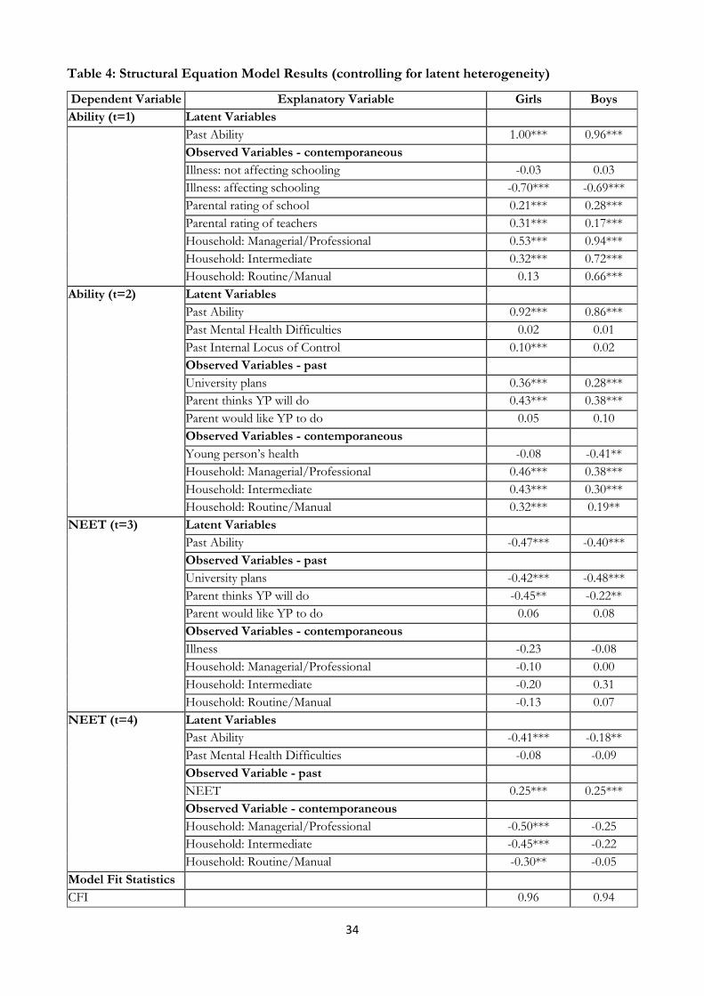
34

Table 4: Structural Equation Model Results (controlling for latent heterogeneity)

Dependent Variable Explanatory Variable Girls Boys

Ability (t=1) Latent Variables

Past Ability 1.00*** 0.96***

Observed Variables - contemporaneous

Illness: not affecting schooling -0.03 0.03

Illness: affecting schooling -0.70*** -0.69***

Parental rating of school 0.21*** 0.28***

Parental rating of teachers 0.31*** 0.17***

Household: Managerial/Professional 0.53*** 0.94***

Household: Intermediate 0.32*** 0.72***

Household: Routine/Manual 0.13 0.66***

Ability (t=2) Latent Variables

Past Ability 0.92*** 0.86***

Past Mental Health Difficulties 0.02 0.01

Past Internal Locus of Control 0.10*** 0.02

Observed Variables - past

University plans 0.36*** 0.28***

Parent thinks YP will do 0.43*** 0.38***

Parent would like YP to do 0.05 0.10

Observed Variables - contemporaneous

Young person’s health -0.08 -0.41**

Household: Managerial/Professional 0.46*** 0.38***

Household: Intermediate 0.43*** 0.30***

Household: Routine/Manual 0.32*** 0.19**

NEET (t=3) Latent Variables

Past Ability -0.47*** -0.40***

Observed Variables - past

University plans -0.42*** -0.48***

Parent thinks YP will do -0.45** -0.22**

Parent would like YP to do 0.06 0.08

Observed Variables - contemporaneous

Illness -0.23 -0.08

Household: Managerial/Professional -0.10 0.00

Household: Intermediate -0.20 0.31

Household: Routine/Manual -0.13 0.07

NEET (t=4) Latent Variables

Past Ability -0.41*** -0.18**

Past Mental Health Difficulties -0.08 -0.09

Observed Variable - past

NEET 0.25*** 0.25***

Observed Variable - contemporaneous

Household: Managerial/Professional -0.50*** -0.25

Household: Intermediate -0.45*** -0.22

Household: Routine/Manual -0.30** -0.05

Model Fit Statistics

CFI 0.96 0.94

35

Dependent Variable Explanatory Variable Girls Boys

RMSEA 0.02 0.02

Notes:

*Significant at 10%; **significant at 5%; ***significant at 1%.

All reported coefficients are standardized. For the continuous covariates, the coefficient represents the change in the dependent variable associated with a 1-SD change in the covariate. For the binary covariates the coefficient represents the change associated with a shift in the variable from 0 to 1.

36

Table 5: Direct and Indirect effects of ability, aspiration, locus of control and health on NEET

Status at age 16/17 (𝒕 = 𝟑) (not controlling for latent heterogeneity)

Variable Girls Boys

Total effect Direct

effect

Indirect

effect

Total effect Direct

effect

Indirect

effect

Ability

Ability (t = 0) -0.16*** - -0.16*** -0.21*** - -0.21***

Ability (t = 1) -0.19*** - -0.19*** -0.25*** - -0.25***

Ability (t = 2) -0.24*** -0.24*** - -0.31*** -0.31*** -

Aspirations

University plans (t=2) -0.08*** - -0.08*** -0.09*** - -0.09***

Parent thinks YP will do (t=2) -0.10*** - -0.10*** -0.12*** - -0.12***

Parent would like YP to do (t=2) -0.01 - -0.01 -0.03 - -0.03

University plans (t=3) 0.39*** 0.39*** - -0.41*** -0.41*** -

Parent thinks YP will do (t=3) 0.41*** 0.41*** - -0.22** -0.22** -

Parent would like YP to do (t=3) 0.02 0.02 - 0.07 0.07 -

Locus of Control

Internal Locus of Control (t=2) -0.02*** -0.02*** -0.01* - -0.01*

Mental Health

Mental Health Difficulties (t=2) 0.02*** - 0.02*** 0.01 - 0.01

General Health

Illness: not affecting schooling (t =1) 0.01 - 0.01 -0.01 - -0.01

Illness: affecting schooling (t =1) 0.14*** - 0.14*** 0.18*** - 0.18***

Young person’s health (t =2) 0.03 - 0.03 0.11** - 0.11**

Illness (t=3) -0.26 -0.26 - -0.02 -0.02 -

Notes: *Significant at 10%; **significant at 5%; ***significant at 1%. All reported coefficients are standardized. For the continuous covariates, the coefficient represents the change in the dependent variable associated with a 1-SD change in the covariate. For the binary covariates the coefficient represents the change associated with a shift in the variable from 0 to 1.

37

Table 6: Direct and Indirect effects of ability and health on NEET Status at age 17/18 (t = 4) (not controlling for latent heterogeneity)

Variable Girls Boys

Total effect Direct

effect

Indirect

effect

Total effect Direct

effect

Indirect

effect

Ability

Ability (t = 0) -0.16*** - -0.16*** -0.11*** - -0.11***

Ability (t = 1) -0.19*** - -0.19*** -0.13*** - -0.13***

Ability (t = 2) -0.24*** -0.15*** -0.09*** -0.16*** -0.02 -0.14***

Aspirations

University plans (t=2) -0.08*** - -0.08*** -0.05*** - -0.05***

Parent thinks YP will do (t=2) -0.10*** - -0.10*** -0.06*** - -0.06***

Parent would like YP to do (t=2) -0.01 - -0.01 -0.01 - -0.01

University plans (t=3) -0.15*** - -0.15*** -0.18*** - -0.18***

Parent thinks YP will do (t=3) -0.16*** - -0.16*** -0.09* - -0.09*

Parent would like YP to do (t=3) 0.01 - 0.01 0.03 - 0.03

Locus of Control

Internal Locus of Control (t=2) -0.02*** - -0.02*** -0.01* - 0.01*

Mental Health

Mental Health Difficulties (t=2) 0.02*** - 0.02*** 0.00 - 0.00

Mental Health Difficulties (t=3) 0.16*** 0.16*** - 0.09** 0.09** -

General Health

Illness: not affecting schooling (t =1) 0.01 - 0.01 0.00 - 0.00

Illness: affecting schooling (t =1) 0.14*** - 0.14*** 0.09*** - 0.09***

Young person’s health (t =2) 0.03 - 0.03 0.06* - 0.06*

Illness (t=3) -0.10 -0.10 - -0.01 -0.01 -

Notes: *Significant at 10%; **significant at 5%; ***significant at 1%.

All reported coefficients are standardized. For the continuous covariates, the coefficient represents the change in the

dependent variable associated with a 1-SD change in the covariate. For the binary covariates the coefficient represents the

change associated with a shift in the variable from 0 to 1.

38

Table 7: Direct and Indirect effects of ability, aspiration, locus of control and health on NEET

Status at age 16/17 (t = 3) (controlling for latent heterogeneity)

Variable Girls Boys

Total effect Direct

effect

Indirect

effect

Total effect Direct

effect

Indirect

effect

Ability

Ability (t = 0) -0.43*** - -0.43*** -0.33*** - -0.33***

Ability (t = 1) -0.43*** - -0.43*** -0.34*** - -0.34***

Ability (t = 2) -0.47*** -0.47*** - -0.40*** -0.40*** -

Aspirations

University plans (t=2) -0.17*** - -0.17*** -0.11*** - -0.11***

Parent thinks YP will do (t=2) -0.20*** - -0.20 -0.15*** - -0.15***

Parent would like YP to do (t=2) -0.02 - -0.02 -0.04 - -0.04

University plans (t=3) -0.42*** -0.42*** - -0.48*** -0.48*** -

Parent thinks YP will do (t=3) -0.45** -0.45** - -0.22** -0.22** -

Parent would like YP to do (t=3) 0.06 0.06 - 0.08 0.08 -

Locus of Control

Internal Locus of Control (t=2) -0.05** - -0.05** -0.01 - -0.01

Mental Health

Mental Health Difficulties (t=2) -0.01 - -0.01 0.00 - 0.00

General Health

Illness: not affecting schooling (t =1) 0.01 - 0.01 -0.01 - -0.01

Illness: affecting schooling (t =1) 0.30*** - 0.30*** 0.24*** - 0.24***

Young person’s health (t =2) 0.04 - 0.04 0.16** - 0.16**

Illness (t=3) -0.23 -0.23 - -0.08 -0.08 -

Notes: *Significant at 10%; **significant at 5%; ***significant at 1%.

All reported coefficients are standardized. For the continuous covariates, the coefficient represents the change in the dependent variable associated with a 1-SD change in the covariate. For the binary covariates the coefficient represents the change associated with a shift in the variable from 0 to 1.

39

Table 8: Direct and Indirect effects of ability and health on NEET Status at age 17/18 (t = 4)

(controlling for latent heterogeneity)

Variable Girls Boys

Total effect Direct

effect

Indirect

effect

Total effect Direct

effect

Indirect

effect

Ability

Ability (t = 0) -0.48*** - -0.48*** -0.23** - -0.23**

Ability (t = 1) -0.48*** - -0.48*** -0.24** - -0.24**

Ability (t = 2) -0.53*** -0.41*** -0.12** -0.28*** -0.18** -0.10**

Aspirations

University plans (t=2) -0.19*** - -0.19*** -0.08** - -0.08**

Parent thinks YP will do (t=2) -0.22*** - -0.22*** -0.11** - -0.11**

Parent would like YP to do (t=2) -0.03 - -0.03 -0.03 - -0.03

University plans (t=3) -0.10** - -0.10** -0.12*** - -0.12***

Parent thinks YP will do (t=3) -0.11* - -0.11* -0.05* - -0.05*

Parent would like YP to do (t=3) 0.02 - 0.02 0.02 - 0.02

Locus of Control

Internal Locus of Control (t=2) -0.05** - -0.05** -0.01 - -0.01

Mental Health

Mental Health Difficulties (t=2) -0.01 - -0.01 0.00 - 0.00

Mental Health Difficulties (t=3) -0.08 -0.08 - -0.09 -0.09 -

General Health

Illness: not affecting schooling (t =1) 0.01 - 0.01 -0.01 - -0.01

Illness: affecting schooling (t =1) 0.34*** - 0.34*** 0.17** - 0.17**

Young person’s health (t =2) 0.04 - 0.04 0.12* - 0.12*

Illness (t=3) -0.06 - -0.06 -0.02 - -0.02

Notes: *Significant at 10%; **significant at 5%; ***significant at 1%.

All reported coefficients are standardized. For the continuous covariates, the coefficient represents the change in the dependent variable associated with a 1-SD change in the covariate. For the binary covariates the coefficient represents the change associated with a shift in the variable from 0 to 1.

40

Appendix

Table A1: Variable Description

Variable (abbreviation) Wave Description

Outcome Variables

English SATs score (English) Prior to

LSYPE

Continuous variable. Higher score indicates better test results.

Maximum score possible is 39. Maths SATs score (Maths)

Science SATs score (Science)

English SATs score (English) 1

Continuous variable. Higher score indicates better test results.

Maximum score possible is 57. Maths SATs score (Maths)

Science SATs score (Science)

GCSE points score (GCSE points) 3

Continuous variable. Higher score indicates better test results.

Maximum varies according to the number of GCSE’s: 12

GCSE’s, all at A*, is equivalent to 696 points.

GCSE English C or above

(GCSE English)

3

Binary Variable (0-1). 1 = if passed.

GCSE Maths C or above

(GCSE Maths)

Not in Education Employment or

Training (NEET)

4, 5 Binary Variable (0-1).

1 = if not in education, employment or training.

Covariates

Child’s birth weight (Birth weight) 1 Continuous variable. Birth weight in kilograms.

Household Socioeconomic Status:

Managerial/Professional

(Household:

Managerial/Professional)

1, 3, 4, 5 Binary Variable (0-1).

1 = if household reference person has an occupation classified

as managerial or professional according to the National Statistics

Socioeconomic Classification.

Household Socioeconomic Status:

Intermediate

(Household: Intermediate)

1, 3, 4, 5 Binary Variable (0-1).

1 = if household reference person has an occupation classified

as Intermediate according to the National Statistics

Socioeconomic Classification.

Household Socioeconomic Status:

Routine/Manual

(Household: Routine/Manual)

1, 3, 4, 5 Binary Variable (0-1).

1 = if household reference person has an occupation classified

as Routine or Manual according to the National Statistics

Socioeconomic Classification.

School Year Month

1 Ordered categorical variable (1-12). 1 is August 1990, 12

September 1989.

Mother’s Highest Qualification: A

level or above

(Mother: A level or above)

1 Binary Variable (0-1). 1 = if Mother’s highest qualification are

A-levels or above.

Mother’s Highest Qualification:

GCSE or lower level qualification

(Mother: GCSE/lower

qualification)

1 Binary Variable (0-1). 1 = if Mother’s highest qualification are

GCSE’s or a lower level qualification.

Parent’s rating of the young

person’s school (Parental rating of

school)

1 Binary Variable (0-1). 1= if parent rates the school as either

good or very good.

Parent’s satisfaction with teachers

(Parental rating of teachers)

1 Binary Variable (0-1). 1= if parent is either satisfied or very

satisfied with the amount of interest teachers show in their

child.

41

Variable (abbreviation) Wave Description

Ethnicity: White (Base Category) 1 Binary Variable (0-1). 1= if young person’s self-designated

ethnic identity is white.

Ethnicity: Mixed 1 Binary Variable (0-1). 1= if young person’s self-designated

ethnic identity is mixed.

Ethnicity: Indian 1 Binary Variable (0-1). 1= if young person’s self-designated

ethnic identity is Indian.

Ethnicity: Pakistani/Bangladeshi 1 Binary Variable (0-1). 1= if young person’s self-designated

ethnic identity is Pakistani or Bangladeshi.

Ethnicity: Caribbean/African 1 Binary Variable (0-1). 1= if young person’s self-designated

ethnic identity is Caribbean.

Ethnicity: Other 1 Binary Variable (0-1). 1= if young person’s self-designated

ethnic identity is neither white nor one of the ethnicities listed

above.

Locus of control: Decide what will

happen in my life (LC: Decide

Happens)

2 Ordered categorical variable (0-4). Designates Young person’s

agreement with statement “I can pretty much decide what will

happen in my life” 0 if strongly disagree, 4 if strongly agree.

Locus of control: If someone is not

a success it’s usually their fault

(LC: Failure is their fault)

2 Ordered categorical variable (0-4). Designates Young person’s

agreement with statement “If someone is not a success in life, it

is usually their own fault” 0 if strongly disagree, 4 if strongly

agree.

Locus of control: If you work hard

at something you’ll usually succeed

(LC: Work hard usually succeed)

2 Ordered categorical variable (0-4). Designates Young person’s

agreement with statement “If you work hard at something you’ll

usually succeed” 0 if strongly disagree, 4 if strongly agree.

Local Index of Multiple

Deprivation

(as above)

2 Higher score indicates greater level of local area deprivation.

Mental Health (GHQ-12) 2, 4

All 12 questions are coded as binary variables (0-1, the value of 0 is given when the respondent replies with one

of the two more positive responses to the question, the value of 1 is given when the respondent replies with one

of the two more negative responses)

Whether recently lost sleep over worry (Recently lost sleep)

Whether recently felt constantly under strain (Recently under strain)

Whether recently felt couldn’t overcome difficulties (Recent difficulties)

Whether recently felt unhappy and depressed (Recently felt unhappy)

Whether recently been losing confidence (Recently losing confidence)

Whether recently been thinking of themselves as a worthless person (Recently felt worthless)

Whether recently been able to concentrate (Recently able to concentrate)

Whether recently felt they have played a useful part in things (Recently not useful)

Whether recently felt capable of making decisions about things (Recently made decisions)

Whether recently been able to enjoy day to day activities (Recently enjoyed activities)

Whether recently been able to face up to problems (Recently faced up to problems)

Whether recently been feeling reasonably happy (Recently felt happy)

General Health

Health problem or disability not

affecting schooling

(Illness not affecting schooling)

1 Binary Variable (0-1). 0 if no health problem or problem affects

schooling; 1 if have a health problem that does not affect

schooling.

42

Variable (abbreviation) Wave Description

Health problem or disability

affecting schooling

(Illness affecting schooling)

1 Binary Variable (0-1). 0 if no health problem or disability that

affects schooling; 1 if health problem or disability does affect

schooling.

Young Person’s Self-Assessed

Health

(Young person’s health)

3 Binary Variable (0-1). 0 if young person self-assesses health as

fairly good or very good; 1 if young person self-assesses health

as not very good or not good at all.

Health problem or disability

(Illness)

4 Binary Variable (0-1):1 if no health problem or problem affects

daily activities; 0 if no health problem.

Aspirations

Likelihood of young person

applying to university

(University plans)

2, 3 Binary Variable (0-1). 1 if the young person thinks it is fairly

likely or very likely that they will apply to university.

What the parent thinks the young

person will do after compulsory

education

(Parent thinks YP will do)

2, 3 Binary Variable (0-1). 1 if parent thinks the young person will

stay in education when they finish compulsory education.

What the parent would like the

young person to do after

compulsory education

(Parent would like YP to do)

2, 3 Binary Variable (0-1). 1 if parent would like the young person

will stay in education when they finish compulsory education.

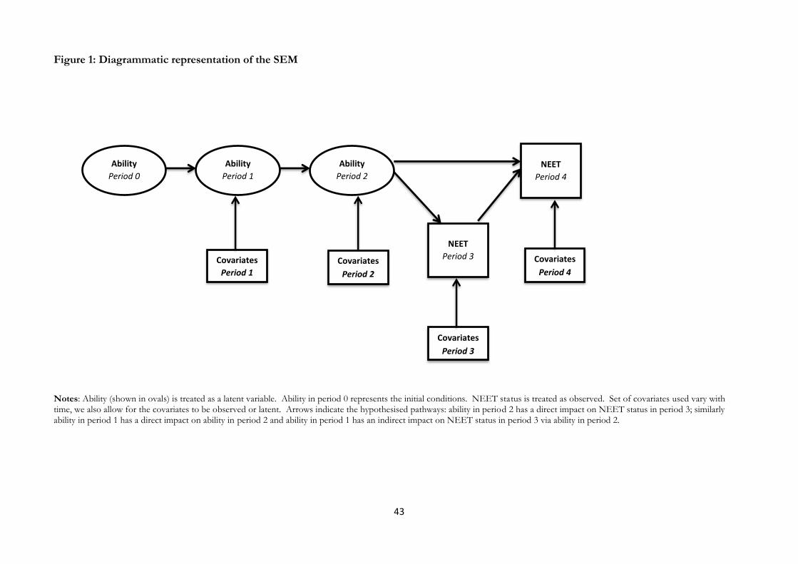
43

Figure 1: Diagrammatic representation of the SEM

Notes: Ability (shown in ovals) is treated as a latent variable. Ability in period 0 represents the initial conditions. NEET status is treated as observed. Set of covariates used vary with time, we also allow for the covariates to be observed or latent. Arrows indicate the hypothesised pathways: ability in period 2 has a direct impact on NEET status in period 3; similarly ability in period 1 has a direct impact on ability in period 2 and ability in period 1 has an indirect impact on NEET status in period 3 via ability in period 2.

Ability

Period 0

Ability

Period 1

Covariates

Period 1

Ability

Period 2

NEET

Period 3

NEET

Period 4

Covariates Period 2

Covariates Period 3

Covariates Period 4

44

Figure 2: Data available across the different waves of the LSYPE

Time t = 0 t = 1 t = 2 t = 3 t = 4

Age 0 to 11 years 11 to 13/14 years 14/15 to 15/16 years 16/17 years 17/18 years

LSYPE wave

Wave 1 Wave 1 Wave 2 Wave 3 Wave 4 Wave 5

Covariates Birth weight

School year month

Mothers education

Ethnicity

Physical Health

Parental rating of school and teachers

Household SES

Mental health

Aspirations

Locus of control

Local index of multiple deprivation

Physical health

Aspirations

Household SES

Mental health

Physical health

Household SES

Household SES

Outcome KS2 (age 11)

(NPD)

KS3 (age 13/14)

(NPD)

KS4-GCSE (age 16/17)

(NPD)

NEET NEET

Notes: SES = Socio economic Status; NPD = National Pupil Database; KS2 = Key Stage 2; KS3 = Key Stage 3; KS4 = Key stage 4; GCSE = General Certificate of Secondary Education; NEET = Not in Education, Employment, or Training.