Journal of Vision (2004) 4, 1120-1135 http://journalofvision.org/4/12/11/ 1120

A detection theory account of change detection

Patrick Wilken Division of Biology, California Institute of Technology,

Pasadena, CA, USA

Wei Ji Ma Division of Biology, California Institute of Technology,

Pasadena, CA, USA

Previous studies have suggested that visual short-term memory (VSTM) has a storage limit of approximately four items. However, the type of high-threshold (HT) model used to derive this estimate is based on a number of assumptions that have been criticized in other experimental paradigms (e.g., visual search). Here we report findings from nine experiments in which VSTM for color, spatial frequency, and orientation was modeled using a signal detection theory (SDT) approach. In Experiments 1-6, two arrays composed of multiple stimulus elements were presented for 100 ms with a 1500 ms ISI. Observers were asked to report in a yes/no fashion whether there was any difference between the first and second arrays, and to rate their confidence in their response on a 1-4 scale. In Experiments 1-3, only one stimulus element difference could occur (T = 1) while set size was varied. In Experiments 4-6, set size was fixed while the number of stimuli that might change was varied (T = 1, 2, 3, and 4). Three general models were tested against the receiver operating characteristics generated by the six experiments. In addition to the HT model, two SDT models were tried: one assuming summation of signals prior to a decision, the other using a max rule. In Experiments 7-9, observers were asked to directly report the relevant feature attribute of a stimulus presented 1500 ms previously, from an array of varying set size. Overall, the results suggest that observers encode stimuli independently and in parallel, and that performance is limited by internal noise, which is a function of set size.

Keywords: feature judgment, visual short-term memory (VSTM), signal detection theory, change blindness, high-threshold theory, capacity limitations

Introduction A critical aspect of any creature’s ability to function ef-

fectively within a changing environment is the facility to efficiently utilize information from a variety of sensory sources in both its present and its immediate past. The high evolutionary value of such information is implied by the ability of human observers to store various perceptual di-mensions, such as spatial frequency, orientation, and hue, with a high degree of fidelity and stability over extended periods of time (Magnussen & Greenlee, 1992; Magnussen, Greenlee, Asplund, & Dyrnes, 1991; Magnussen, Greenlee, & Thomas, 1996; Regan, 1985). It has been shown, for instance, that observers are readily able to detect spatial frequency changes for time periods of upwards of 60 s that are smaller than the Nyquist frequency associated with the spacing between adjacent cones on the fovea (Magnussen, Greenlee, Asplund, & Dyrnes, 1990; Regan, 1985).

In a typical visual short-term memory (VSTM) experiment, observers are presented with two displays, each display composed of a number of spatially distinct stimuli. The two arrays are separated by a short temporal interval, usually greater than 80 ms to avoid attentional capture (Kanai & Verstraten, 2004). Observers are asked to decide whether the two arrays were composed of identical stimuli. Per-formance is believed to be a function of the nature and extent to which a memory of the first display is formed. It is commonly found that an increase in the number of ele-

ments present leads to a monotonic decrease in the sensi-tivity of observers to differences between the two displays; although for experiments employing suprathreshold stim-uli, this decrease is typically only observed after set size has reached around three to four elements (Luck & Vogel, 1997; Pashler, 1988; Vogel, Woodman, & Luck, 2001).

A prominent class of VSTM model proposes that the performance decline associated with increasing set size is caused by a fundamental limit of the number of items that can be encoded, either because the capacity of VSTM itself is limited (Cowan, 2001; Luck & Vogel, 1997; Pashler, 1988; Vogel et al., 2001), or because of a bottleneck in the number of items that can be attended to during the encod-ing process (Rensink, 2000).

This type of model assumes that VSTM is restricted in storage capacity to only a few items, C (often estimated to lie in the range of 4 to 5), within a set size N (Pashler, 1988). The probability that a suprathreshold change will be reported (H) is then

1 for ;

1 for ,

H N C

C CH F NN N

C

= <

= + − ≥

(1)

where F is the probability on a given trial that an observer will incorrectly guess “change” when no change has oc-curred. This model classically envisages VSTM as a single high-level store within which items, often conceived as

doi:10.1167/4.12.11 Received June 28, 2004; published December 29, 2004 ISSN 1534-7362 © 2004 ARVO

Journal of Vision (2004) 4, 1120-1135 Wilken & Ma 1121

bundles of perceptual features, are stored. This type of high-threshold (HT) model has been shown to be based on a num-ber of unattractive assumptions (Macmillan & Creelman, 1991), and its applicability has been questioned for other experimental paradigms, such as visual search (Eckstein, Thomas, Palmer, & Shimozaki, 2000; Palmer, 1995; Palmer, Verghese, & Pavel, 2000). First, it posits that the relevant information used to determine whether a visual object has been seen previously is encoded as a discrete unit within the brain (i.e., the item is simply present or not, in the absence of internal noise). Second, it assumes that the internal state engendered in the absence of an item can never contribute to an “item seen” response (i.e., distracters can never produce enough misleading evidence to elicit a false positive answer). Detection theory accounts, which suggest a continuous model of perceptual encoding, are more natural from a cortical viewpoint (Verghese, 2001). In these models, each encoded item is internally represented by a continuous variable, usually with added Gaussian noise, that is positioned within a multidimensional percep-tual space.

The purpose of the present study was to determine how well a detection theory framework could account for the basic finding of a performance decline as a function of set size reported within the VSTM literature, and whether this type of model offered alternative insights into the processes leading to this limitation. Our findings suggest that theo-retical models that conjecture a high-level storage bottle-neck, such as working memory, are unnecessarily complex, and that the assumption of neuronal noise, in conjunction with a simple decision rule, provides a more satisfactory framework to understand VSTM than current HT ac-counts.

Layout of study This report summarizes the results of nine experiments.

These experiments fall naturally within three groups; each group is composed of three independent experiments in which the critical feature space manipulated was color, ori-entation, or spatial frequency.

The first group involves a standard set-size manipula-tion used in many VSTM experiments (e.g., Luck & Vogel, 1997; Vogel et al., 2001). These results confirmed that our paradigm produces results consistent with those reported previously in the literature. In addition to the standard analysis, confidence ratings were collected, allowing us to generate receiver operating characteristics (ROCs). Compared with the current HT account, detection theory models pro-vided a much better match between theoretical predictions and the observed ROCs. This analysis suggested the key factor limiting performance was an increase in noise in the encoded representation of each stimulus element with in-creasing set size.

The second group of experiments kept set size con-stant, but systematically varied target number, allowing us

to systematically vary performance while keeping encoding noise constant. This allowed a reduction in the necessary parameter space needed to model the empirical ROCs, and thus a stricter evaluation of the detection theory account.

The third group of experiments attempted to measure the encoding noise in a more direct manner. In these ex-periments, rather than requiring observers to report in a yes/no manner whether a change had occurred, observers were asked to manipulate a scalar probe to match the rele-vant feature property of a previously memorized item in an array of variable set size. These experiments, independent of a detection theory analysis, confirmed the increase in noise in the representations of encoded items as a function of set size.

Methods

Participants Fifteen observers participated in each experiment re-

ported in this study. Participants were all students or staff at the California Institute of Technology, aged between 18 and 35 years, with normal or corrected-to-normal acuity, and by self-report normal color vision.

Apparatus Stimuli were generated in Matlab, using Psychophysics

Toolbox extensions (Brainard, 1997; Pelli, 1997), and were presented using an Apple G4 computer, with a 128-bit AGP Graphics card, running Mac OS 9.2.2. They were pre-sented on a 21-inch Apple Studio Design monitor, with a resolution of 1024 x 768 pixels, and a refresh rate of 120 Hz.

Experiments 1-6

Stimuli

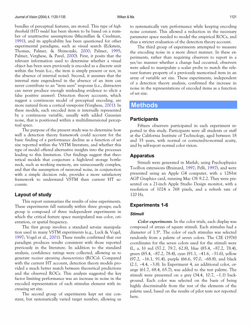
Color experiments. In the color trials, each display was composed of arrays of square stimuli. Each stimulus had a diameter of 1.5º. The color of each stimulus was selected randomly from a palette of seven colors. The CIE (1976) coordinates for the seven colors used for the stimuli were (L, a, b) red (57.2, 79.7, 62.8), blue (85.4, –87.2, 78.4), green (85.4, –87.2, 78.4), cyan (91.1, –41.6, –31.6), yellow (97.2, –16.1, 91.4), purple (66.6, 97.0, –68.8), and black (2.1, –4.4, –3.8). In Experiment 4, an additional color, or-ange (61.7, 68.4, 65.7), was added to the test palette. The stimuli were presented on a grey (34.4, 10.7, –1.1) back-ground. Each color was selected on the basis of being highly discriminable from the rest of the elements of the palette used, based on the results of pilot tests not reported here.

Journal of Vision (2004) 4, 1120-1135 Wilken & Ma 1122

Figure 1. Schematic of a single experiments, the colored square

Orientation and spatial frequency experiments. The orientation and spatial frequency stimulus elements used were Gabor patches. The phase of each Gabor, both within and across arrays, was randomized. The SD of the Gaussian envelope used was 11 pixels, and had a peak amplitude of 32.3 cd/m2.

The orientation stimuli had a wavelength of 16 pix-els/cycle, which was equivalent to 0.2º. In the orientation experiments, the initial orientation of each stimulus ele-ment was assigned at random. If a change occurred to a stimulus element, there was an equal probability of its ori-entation being either incremented or decremented by an angle of π/4 or π/2.

In the spatial frequency experiments, the orientation of each stimulus element was 0º (i.e., vertical). Each stimulus element had an equal probability of being composed of one of three possible wavelengths (8, 16, or 32 pixels/cycle). If a change occurred, there was an equal probability of the change stimulus adopting either of the two remaining spa-tial frequency values.

Placement of stimuli. The head position of observers was unfixed, and viewing distance was on average 66 cm from the display. Stimuli were presented at N equally spaced points, around an imaginary circle of diameter 14.4º (see Figure 1 for a schematic of the placement of the stim-uli). The number of locations, N, within the circle was equal to the maximum possible number of stimuli that could be present within an array from a particular experi-ment (i.e., N = 8 for color and spatial frequency and N = 6 and 5 for orientation, for the set-size and target-number experiments, respectively). If, in Experiments 1-3, less than the maximum number of possible stimuli was present within an array (i.e., set size within a trial was less than N),

the stimuli were placed randomly on a subset of the possi-ble stimulus locations. The minimum spacing between ad-jacent stimuli (i.e., when N = 8) was 6.5º. All stimuli were displayed on a dark grey background (2.3 cd/m2).

Procedure In Experiments 1-3, set size was varied (N = 2, 4, 6, and

8 for color and spatial frequency and N = 2, 3, 4, and 5 for orientation), while number of targets (T = 1) was kept con-stant. In Experiments 4-6, set size was kept constant (N = 8 for color and spatial frequency and N = 6 for orientation), while the number of possible targets was systematically var-ied (T = 1, 2, 3, and 4).

Data were collected from participants over two ses-sions. Each session consisted of five blocks, and each block was composed of 128 trials. The order of trials within all blocks was counterbalanced using an ABBA design. In Ex-periments 1-3, trials were counterbalanced for set size and change/no-change trials; In Experiments 4-6, trials were counterbalanced for target number and change/no-change trials. The position of each stimulus was randomly assigned on a trial-by-trial basis.

Participants were seated in a dimly lit room. Trials be-gan with the presentation of a fixation point, in the form of a small cross (0.2º x 0.2º), placed at the center of the dis-play. At 250 ms after the onset of the fixation cross, the first array of stimuli was presented for 100 ms. After the offset of the first array, the screen remained blank for 1500 ms. Immediately thereafter a second array was pre-sented for 100 ms. Overall there was a probability of .5 that within a particular trial the two arrays would be composed of stimuli identically matched in the appropriate feature dimension. In Experiments 4-6, on any change trial, there was an equal probability that the change would involve one, two, three, or four stimuli.

trial used for the set size and the target number experiments. In the orientation and spatial frequencys were replaced with Gabor patches.

+

+

+100 ms

1500 ms

100 ms

Change?

Confidence?

Journal of Vision (2004) 4, 1120-1135 Wilken & Ma 1123

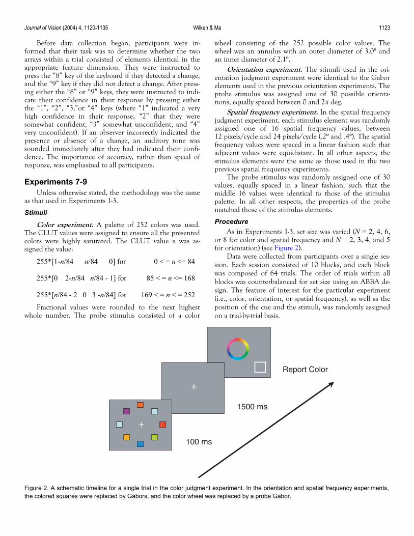
Figure 2. A schematic timeline for a single trial in the color judgment experiment. In the orientation and spatial frequency experiments,the colored squares were replaced by Gabors, and the color wheel was replaced by a probe Gabor.

Before data collection began, participants were in-formed that their task was to determine whether the two arrays within a trial consisted of elements identical in the appropriate feature dimension. They were instructed to press the “8” key of the keyboard if they detected a change, and the “9” key if they did not detect a change. After press-ing either the “8” or “9” keys, they were instructed to indi-cate their confidence in their response by pressing either the “1”, “2”, “3,”or “4” keys (where “1” indicated a very high confidence in their response, “2” that they were somewhat confident, “3” somewhat unconfident, and “4” very unconfident). If an observer incorrectly indicated the presence or absence of a change, an auditory tone was sounded immediately after they had indicated their confi-dence. The importance of accuracy, rather than speed of response, was emphasized to all participants.

Experiments 7-9 Unless otherwise stated, the methodology was the same

as that used in Experiments 1-3.

Stimuli

Color experiment. A palette of 252 colors was used. The CLUT values were assigned to ensure all the presented colors were highly saturated. The CLUT value n was as-signed the value:

255*[1-n/84 n/84 0] for 0 < = n <= 84

255*[0 2-n/84 n/84 - 1] for 85 < = n <= 168

255*[n/84 - 2 0 3 -n/84] for 169 < = n < = 252

Fractional values were rounded to the next highest whole number. The probe stimulus consisted of a color

wheel consisting of the 252 possible color values. The wheel was an annulus with an outer diameter of 3.0º and an inner diameter of 2.1º.

Orientation experiment. The stimuli used in the ori-entation judgment experiment were identical to the Gabor elements used in the previous orientation experiments. The probe stimulus was assigned one of 30 possible orienta-tions, equally spaced between 0 and 2π deg.

Spatial frequency experiment. In the spatial frequency judgment experiment, each stimulus element was randomly assigned one of 16 spatial frequency values, between 12 pixels/cycle and 24 pixels/cycle (.2º and .4º). The spatial frequency values were spaced in a linear fashion such that adjacent values were equidistant. In all other aspects, the stimulus elements were the same as those used in the two previous spatial frequency experiments.

The probe stimulus was randomly assigned one of 30 values, equally spaced in a linear fashion, such that the middle 16 values were identical to those of the stimulus palette. In all other respects, the properties of the probe matched those of the stimulus elements.

Procedure As in Experiments 1-3, set size was varied (N = 2, 4, 6,

or 8 for color and spatial frequency and N = 2, 3, 4, and 5 for orientation) (see Figure 2).

Data were collected from participants over a single ses-sion. Each session consisted of 10 blocks, and each block was composed of 64 trials. The order of trials within all blocks was counterbalanced for set size using an ABBA de-sign. The feature of interest for the particular experiment (i.e., color, orientation, or spatial frequency), as well as the position of the cue and the stimuli, was randomly assigned on a trial-by-trial basis.

+

+

100 ms

1500 ms

Report Color

Journal of Vision (2004) 4, 1120-1135 Wilken & Ma 1124

Trials began with the presentation of a fixation point, in the form of a small cross (0.2º x 0.2º), placed at the cen-ter of the display. At 250 ms after the onset of the fixation cross, the array of stimuli was presented for 100 ms. After the offset of the first array, the screen remained blank for 1500 ms. Immediately thereafter a square cue (3º x 3º, composed of lines 1 pixel wide) was centered around the location of one of the previously presented items. At the same time, a test probe was displayed centrally. Both the test probe and the cue remained present until the trial was finished.

Before data collection began, participants were in-formed that their task was to match as closely as possible the relevant stimulus property of the probe stimulus with that of the stimulus at the cued location. In the color ex-periment, they were asked to indicate the cued stimulus property by using the mouse to point and click at the part of the color-wheel that most closely matched the feature property of the cued stimulus. In the orientation experi-ment, participants were instructed to match the cued fea-ture property by using the right and left arrows on the key-board to rotate the probe Gabor (clockwise and counter-clockwise, respectively). In the spatial frequency experi-ment, participants also used the arrow keys on the key-board to change the spatial frequency of the probe stimulus (the right arrow increasing the spatial frequency, left arrow decreasing it). In the orientation and spatial frequency ex-periments, observers recorded their responses by pressing the space bar on the keyboard. As in previous experiments, the importance of accuracy, rather than speed of response, was emphasized to all participants.

Detection theory models of change Depending on the nature of the decision process, de-

tection theories can be divided into either first-order or sec-ond-order integration models (Shaw, 1982). In first-order inte-gration accounts, the relevant information from each stimulus is pooled, and a single decision is made on that combined information. Conversely, in second-order mod-els, a separate decision is made on each relevant stimulus attribute, and a final response is based on the assimilation of these decisions (Palmer et al., 2000). Here we consider two general accounts of VSTM based on prototypical ex-amples of first-order or second-order integration models. Full technical details of the detection theory and HT mod-els used can be found in Appendix A.

Maximum absolute differences model The maximum absolute differences model (MAD) is a de-

tection theory generalization of an HT account previously reported by one of the authors (Wilken, 2001), and is based closely on Shaw’s (1980) independent decisions model. In this class of second-order integration model (Palmer,

1990; Shaw, 1980), an observer attempting to detect a change among N elements is considered to be monitoring N noisy channels, each channel representing information associated with a single item within the display. A change in an item will be reflected in a change in the signal of one of the channels. If the alteration in this signal is greater than a particular threshold, a change will be reported. It is further assumed that decisions across channels are inde-pendent, and hence N independent decisions are made about N elements within a display. Because the signal in each channel is noisy, there is a certain probability that the signal in a non-change channel will pass above the detec-tion threshold and a change will be reported erroneously.

Here we assume that it is the absolute size of this change that is important for the detection of change, and not its sign (e.g., a change from red to green will be as read-ily detected as a change from green to red). Such a differ-encing operation is common in describing classical same-different tasks (Macmillan & Creelman, 1991), and is the simplest operation of its kind. This assumption of the MAD model leads to a somewhat different mathematical exposition from the max model variant (Eckstein et al., 2000; Palmer, 1990, 1995; Palmer et al., 2000; Shaw, 1980) previously employed to explain performance in visual search tasks.

Moreover, we assume a fixed effective distance in stimulus representation space (and thus sensitivity) between different stimuli at one location in the two displays. It should be noted that by doing this, we collapse all repre-sented magnitudes of individual changes (e.g., a transition from red to green versus one from red to orange); however, we do expect their differences to translate into differences in performance.

Within the MAD model, the typical finding that an in-crease in set size leads to a monotonic decline in perform-ance in VSTM tasks can be attributed to two potential causes. First, increases in the number of channels being monitored will lead to an increase in the likelihood that noise within a non-change channel will be mistakenly at-tributed to an actual change (i.e., decisional noise). Second, independent of decisional noise, increases in set size may amplify the noise present within each channel. For in-stance, the assumption that observers are limited by a fixed number of samples they can extract from a visual scene, N, leads to a prediction from central limit theorem that noise within each (equally) monitored channel will increase pro-portional to N, because the number of samples per channel will then be proportional to 1/N (Palmer, 1990). Naturally, other assumptions will lead to different changes in internal noise as a function of N. Here we take an agnostic viewpoint, and retain a single free parameter as our noise estimate within a single monitored channel. In cases in which change involves a single target element, the MAD model approximates the performance of an ideal observer (Palmer et al., 2000).

Journal of Vision (2004) 4, 1120-1135 Wilken & Ma 1125

High-Threshold

Max Absolute Difference (MAD)

Sum Absolute Difference (SAD)

Absolute Difference

Noisy Internal RepresentationNoisy Internal Representation

DecisionDecisionMAX RuleMAX RuleStimuliStimuli

Absolute Difference

Noisy Internal RepresentationNoisy Internal Representation

DecisionDecisionSUMStimuliStimuli

DecisionStimuliStimuliGuessing

Limited Capacity Store

Sum of absolute differences model In addition to the MAD model, a sum of absolute differ-

ences model (SAD) was assessed. This first-order integration account shares the MAD model’s assumptions that each stimulus attribute is represented by a noisy internal state, and that a stimulus change is represented by an absolute difference between matched states in the first and second displays. It differs from the MAD model in that it presumes that the absolute differences calculated for each stimulus are summated to form the distribution upon which a single decision is based.

Figure 3 offers a schematic of the information flow in the three models examined in this study.

Change detection as a function of set size

The first three experiments performed a set-size ma-nipulation frequently employed in previous VSTM experi-ments (Vogel et al., 2001). This experimental manipulation allowed us to assess whether our experimental methodology produced results broadly consistent with experimental paradigms that have applied an HT account (Luck & Vo-gel, 1997). However, unlike these previous experiments, confidence ratings were also collected allowing us to gener-ate empirical ROCs that could then be compared with theoretical predictions from the MAD and SAD models of change detection.

Results As shown in Figure 4, there was a general decline in

the ability of observers to detect a change between the first and second arrays, with hit rates monotonically decreasing, and false alarm rates monotonically increasing as a function of set size.

An analysis of the color change data using an HT model (Pashler, 1988) implies a capacity estimate C of 3.80 ± .13 (M ± SE), consistent with previous studies that have

suggested visual working memory for color has a storage capacity of three-to-five items (Cowan, 2001; Luck & Vogel, 1997; Pashler, 1988; Wilken, 2001). An HT analysis for the orientation and spatial frequency data yielded a slightly lower estimate for C (2.58 ± .27, 2.51 ± .18, for orientation and spatial frequency, respectively), but one still in general accord with the broadly agreed upon storage limit of VSTM.

Figure 3. A diagram of the information flow in the HT, SAD, and MAD models.

The confidence-interval data were pooled over observ-ers, and empirical ROCs were obtained for all set sizes. For each model tested, the best-fitting parameters were deter-mined through a multidimensional error-minimization procedure. At every iteration of this minimization, two steps were executed. First, the locations of the criteria for all set sizes were estimated using the empirical response frequencies in the no-change condition and the noise dis-tribution from the model with the parameters values at the current iteration. Next, for each set size, a chi-squared sta-tistic was computed between the average numbers of re-sponses for a single observer in each response category in the change condition and the numbers expected from the model signal distribution with the current parameter values and the estimated criterion locations. These chi-squared values were summed over set sizes, and their sum was minimized using an algorithm provided by Matlab (The Mathworks, Inc.) based on the Nelder-Mead simplex (direct search) method. To correct for problems associated with pooling across nonlinear data sets, and to obtain error bars for the parameter estimates, a jackknife procedure was em-ployed (Quenouille, 1949; Tukey, 1958). The goodness of the resulting fit was measured by the above-mentioned total chi-squared statistic.

We first attempted to fit the ROC data using the stan-dard HT model described in Equation 1. As can be seen in Figure 4, the empirical ROCs were regular in shape, quite unlike the theoretical straight lines predicted by HT ac-counts (Swets, 1986a, 1986b). Not surprisingly, as can be seen in Table 1, the resulting HT fit was very poor.

Journal of Vision (2004) 4, 1120-1135 Wilken & Ma 1126

2 4 6 80

0.250.5

0.751

Set Size

Color

0 0.5 10

0.5

1

Hit

Rat

e

0 0.5 10

0.5

1H

it R

ate

0 0.5 10

0.5

1

Hit

Rat

e

0 0.5 10

0.5

1

Hit

Rat

e

False Alarm Rate

Set Size2 4 6 8

00.25

0.50.75

1

Set Size

Spatial Frequency

0 0.5 10

0.5

1

0 0.5 10

0.5

1

0 0.5 10

0.5

1

0 0.5 10

0.5

1

False Alarm Rate

Set Size2 3 4 5

00.25

0.50.75

1

Set Size

Orientation

0 0.5 10

0.5

1

0 0.5 10

0.5

1

0 0.5 10

0.5

1

0 0.5 10

0.5

1

False Alarm Rate

Set Size

Hits &False Alarms

High-ThresholdModel

MAD with Variable Noise

SAD withVariable Noise

MAD withConstant Noise

Figure 4. Raw data plus model fits for the color, orientation, and spatial frequency set-size experiments. Top row shows overall hit rates(solid line) and false alarm rates (dashed line) for 15 observers. In all cases the SE bars fall within the circular symbols. The lower fourrows show example model fits for the HT model, MAD with constant noise and equal variance, and SAD and MAD with the variablenoise and equal variance assumptions. Different symbols represent performance at different set sizes: set-size 2 for color, orientationand SF – red stars; set-size 4 for color and SF, set-size 3 for orientation – green triangles; set-size 6 for color and SF, set-size 4 fororientation – blue circles; set-size 8 for color and SF, set-size 5 for orientation – purple squares.

Type of model Constant noise

Equal variance

Color χ2 (df)

Orientation χ2 (df)

SF χ2 (df)

HT - - >2503 (27) >305 (27) >310 (27)

MAD Yes Yes 120 (27) 50.5 (26) 81.4 (27)

Yes No 119 (26) 48.2 (25) 79.5 (26)

No Yes 32.8 (24) 28.2 (23) 36.0 (24)

No No 26.6 (20) 22.6 (19) 34.3 (20)

SAD Yes Yes 94.4 (27) 53.4 (26) 85.5 (27)

Yes No 43.0 (26) 52.0 (25) 54.6 (26)

No Yes 40.6 (24) 31.0 (23) 60.8 (24)

No No 21.5 (20) 29.6 (19) 27.2 (20)

Table 1. Results of parameter fitting for HT, MAD, and SAD models for the variable set-size experiments.

Journal of Vision (2004) 4, 1120-1135 Wilken & Ma 1127

SDT accounts offer a rich theoretical basis with which to understand the effects of set size on performance in VSTM tasks. We assessed how well decisional noise alone could account for changes in performance with set size (our constant-noise condition), and whether allowing noise to increase with set size generated a significantly better fit for the observed ROCs (our variable-noise condition). In addi-tion, we assessed whether allowing the variances of the change and the no-change distributions to differ provided a significantly better fit to the observed distributions, as previous studies have shown that the assumption of equal variance between signal and noise distributions is often violated (Swets, 1986a, 1986b).

The ROCs in our SDT models are determined by the effective perceptual distance, d, between different stimuli at one location in the two displays (unlike the usual sensitivity parameter d’, this does not assume equal and unitary vari-ances), and the amount of noise in their representations. For color and spatial frequency, all SDT models have a re-dundant scaling parameter, which we use to fix d. In our models, d is assumed to be constant across changes in set size. This leaves our constant-noise model with a single free parameter, the SD of the noise, and for the variable-noise models four parameters, the SDs of the noise associated with each set size. However, for orientation, because the stimulus space is circular, there is no such scaling, and we always estimate the effective distance d together with the parameter(s) of the noise (see Appendix A for a discussion

of the measurement of noise in von Mises distributions). Thus, the SDT models in the orientation paradigm have one degree of freedom less than those in the color and spa-tial frequency paradigms.

Before discussing the relative effectiveness of various SDT models to account for the ROC data, it is important to note that all SDT accounts offered better fits to the ROC data than the standard HT model. Moreover, this result cannot be solely attributed to a larger parameter space used by the SDT accounts. Even when the SDT ac-counts shared the same degrees of freedom as the HT ac-counts, the fit for the SDT models was much better (χ2 equal to 2503 vs. 120 and 94, for HT vs. MAD and SAD for the color experiment; χ2 equal to 305 vs. 50.5 and 53.4 for HT vs. MAD and SAD for the spatial frequency ex-periment).

Next, within-model comparisons were performed to as-sess whether the reduction in the χ2 values associated with rejecting the constant noise assumption could be explained purely as a result of the increase in the parameter space (see Wickens, 2002, for an explanation of this technique). This analysis showed that even when taking the increase in the size of the parameter space into account, for both MAD and SAD, the model fit was significantly better when the assumption of constant noise was relaxed (p < .001 for all comparisons, no correction for multiple comparisons). Figure 5 shows the change in the noise parameter for the MAD model. In all three feature modalities, the increase in

2 4 6 80.2

0.25

0.3

0.35

0.4

0.45

0.5

Set Size

Par

amet

er o

f Noi

se (

units

of

)

Color

2 3 4 50.45

0.5

0.55

0.6

0.65

0.7

0.75

Set Size

Orientation

2 4 6 80.3

0.35

0.4

0.45

0.5

0.55

0.6

Set Size

Spatial Frequency

d

Figure 5. Behavior of the noise estimated from the MAD equal-variance model as a function of set size. For color and spatial fre-quency, the plot shows the SD of the noise in units of the effective distance d described in the text. For orientation, the plot shows theequivalent parameter s (see Appendix A, Equation 5) in units of the estimated d.

Journal of Vision (2004) 4, 1120-1135 Wilken & Ma 1128

noise is monotonic and roughly linear. This strongly sug-gests that as more items are encoded, the encoding of each item becomes noisier.

A similar evaluation was performed to assess the rela-tive improvement in χ2 associated with relaxing the equal variance assumption. In this case, no significant change in χ2 was found for the MAD fits for any of the experiments, or for the SAD fit for orientation (p > .05), whereas a sig-nificant improvement was found for SAD fits for color and spatial frequency (p < .001 for both comparisons).

Change detection as a function of target number

The results of the set-size experiments supported the value of a detection theory approach for modeling per-formance in VSTM tasks, with both the SAD and MAD models providing good fits to the experimental data. These experiments suggest that the noise of the internal percept increases monotonically as a function of set size.

Given these results, we decided to perform a second set

of experiments in which set size was fixed (N = 8 for color and spatial frequency and N = 6 for orientation), but per-formance systematically varied by changing the target num-ber (T = 1, 2, 3, or 4). This manipulation had two main advantages: first, it allowed an assessment of the robustness of the SDT approach when performance was varied in quite different manner; and second, by fixing set size (and therefore, presumably, internal noise) it allowed a substan-tial reduction in the necessary parameter space needed for modeling, in turn allowing a more sensitive comparison between models.

Results Performance improved as a function of the number of

elements changing, as demonstrated by the monotonically increasing hit rates as a function of target number shown in Figure 6.

Experiments 4-6 were analyzed in a similar manner to Experiments 1-3, with the essential difference that only one noise parameter was used for all four ROCs, because set size was kept constant.

2 4 6 80

0.250.5

0.751

Target Number

Color

0 0.5 10

0.5

1

Hit

Rat

e

0 0.5 10

0.5

1

Hit

Rat

e

0 0.5 10

0.5

1

Hit

Rat

e

False Alarm Rate

3 4 5 60

0.250.5

0.751

Target Number

Orientation

0 0.5 10

0.5

1

0 0.5 10

0.5

1

0 0.5 10

0.5

1

False Alarm Rate

2 4 6 80

0.250.5

0.751

Target Number

Spatial Frequency

0 0.5 10

0.5

1

0 0.5 10

0.5

1

0 0.5 10

0.5

1

False Alarm Rate

Hits &False Alarms

High-ThresholdModel

MAD with Variable Noise

SAD withVariable Noise

Figure 6. Raw data plus model fits for the color, orientation, and spatial frequency target-number experiments. Top row shows overallhit rates (solid line) and false alarm rates (dashed line) for 15 observers. In all cases the SE bars fall within the circular symbols. Ex-periments generated only one false alarm rate; for comparison purposes, the same false alarm rate is shown for each target numbercondition. The lower three rows provide example model fits for the HT model, and SAD and MAD with variable noise and unequal vari-ance assumptions. Symbols represent performance in the different target number conditions: one target – red stars; two targets – greentriangles; three targets – blue circles; and four targets – purple squares.

Journal of Vision (2004) 4, 1120-1135 Wilken & Ma 1129

An analysis of the color change data was performed, us-ing a modified form of the HT model (Pashler, 1988) to take into account variations in target number, and this model implied capacity estimates of C of 2.35 ± .14 for color, 1.79 ± .17 for orientation, and 2.27 ± .26 for spatial frequency. These results again are broadly consistent with previous estimates of the storage of visual working memory (Cowan, 2001; Luck & Vogel, 1997; Pashler, 1988; Wilken, 2001).

As can be seen in Figure 6, the empirical ROCs were regular in shape, again quite unlike the straight lines pre-dicted by HT accounts (Swets, 1986b).

An examination of Table 2 makes a number of points immediately apparent. As in the set-size experiments, the fit of the HT model is much worse across all experiments compared to the fits associated with SAD and MAD mod-els. Once more, the MAD model in general offers a better fit for the data than the SAD model (the only exception being the analysis of the orientation experiment, under the equal variance assumption).

Contrasting with the results of the previous set-size ex-periments, a within-model analysis found that there was a significant reduction in χ2 values associated with relaxing the equal variance assumption for all MAD model fits (p < .001 for color and orientation and p < .01 for spatial frequency). Removing the equal variance assumption was also found to significantly improve the SAD model fits for the color (p < .001) and orientation (p < .05) experiments.

Why was there stronger evidence against the equal variance assumption in the target number experiments, than in the set-size experiments? We can think of at least two reasons. First, by keeping the set size constant, we were able to perform a more sensitive test of the change in χ2 values. Perhaps more crucially, it would be expected that if in fact the change and no change distributions were un-equal, that this would become more apparent as the num-ber of targets with the display increased.

An estimation of the internal representation

Explicit within the MAD and SAD models is the as-sumption that change detection is a process of comparison between stored elements of the first array with correspond-ing elements within the second array. As such, the second array can be considered a complex probe into the informa-tion encoded for each element within the first array. This probe is necessarily complex, requiring comparisons across all elements in the first encoded array and their matching elements within the second probe array, with a correspond-ing decision rule needed to determine whether stimulus elements differ between the first and second arrays.

The results of the set-size experiments suggest that change becomes harder to detect as a function of increasing

set

s on the previous set-size experiments, with the

s ee judgment experiments show a consistent pic-

the

all u

size primarily as a function of increasing noise within the stored representation of each stimulus element. Given that the detection theory account is broadly correct, it should be possible to directly show, as a function of set size, an increase in noise for the feature properties of a single encoded element, without inferring these indirectly from the responses generated when observers are required to make comparisons across multiple stimulus elements be-tween arrays.

The following three judgment experiments were essen-tially variation

Type of model

Constant noise

Equal variance

Color χ2 (df)

Orientationχ2 (df)

SF χ2 (df)

HT - - 979 (27) 322 (27) 898 (27)

MAD Yes Yes 66.1 (27) 54.1 (26) 63.4 (27)

Yes No 18.9 (26) 28.6 (25) 57.4 (26)

SAD Yes Yes 138.6 (27) 35.7 (26) 75.5 (27)

Yes No 25.4 (26) 30.7 (25) 74.9 (26)

Table 2. Results of parameter fitting for HT, MAD, and SAD models for variable target number experiments.

following major modification: rather than using a sec-ond array as a probe of change detection, at the time when the second array would have appeared, the location of a single element within the first array was cued, and observ-ers were asked to modify the feature properties of a probe item to match those of the cued element (these experiments were inspired by earlier work by Prinzmetal and colleagues [Prinzmetal, Amiri, Allen, & Edwards, 1998; Prinzmetal, Nwachuku, Bodanski, Blumenfeld, & Shimizu, 1997]). This method greatly simplifies the decision process, and avoids the necessity of observers having to perform multiple comparisons across stored stimulus items. The demonstra-tion of a monotonic increase in noise of a single item as a function of set size in this task would offer strong inde-pendent support for the detection model account of VSTM.

ResultThe thr

ture: with increasing set size, the variance of the estimate of cue feature rises in a monotonic fashion. As shown in

Figure 7, this increase in noise shows an approximately lin-ear trend when measured in terms of standard deviation.

It is important to note that HT accounts predict a very different pattern of results: noise should increase little if at

ntil working memory capacity was full, at which point observer’s judgment noise should show a sudden increase as observers start to guess on a certain proportion of trials the relevant stimulus attribute. No such abrupt change in the noise is evident in the data.

Journal of Vision (2004) 4, 1120-1135 Wilken & Ma 1130

to that observed in the set size

Observers showed no systematic bias in their estimates ientation. Interestingly, observers did

sho

mean. A trivial expla-nation of this result might be expected to hold if observers

wer

an internal template based on prior experience, perh

2 4 6 8

0

20

40

60

80

Set Size

Judg

emen

t Err

or

0

300

Color

0

300

0

300

Fre

quen

cy

-100 -50 0 50 1000

300

Error (clut values)

2 3 4 5

0

20

40

60

Set Size

0

500

Orientation

0

500

0

500

-50 0 500

500

Error (degrees)

2 4 6 80

0.5

1

1.5

2

Set Size

0200

Spatial Frequency

0200

0200

-4 -3 -2 -1 0 1 2 3 40

200

Error (cycles/degree)

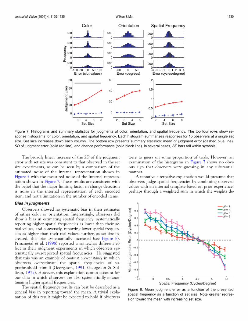
Figure 7. Histograms and summary statistics for judgments of color, orientation, and spatial frequency. The top four rows show re-sponse histograms for color, orientation, and spatial frequency. Each histogram summarizes responses for 15 observers at a single setsize. Set size increases down each column. The bottom row presents summary statistics: mean of judgment error (dashed blue line),SD of judgment error (solid red line), and chance performance (solid black line). In several cases, SE bars fall within symbols.

The broadly linear increase of the SD of the judgment error with set size was consistent

experiments, as can be seen by a comparison of the estimated noise of the internal representation shown in Figure 5 with the measured noise of the internal represen-tation shown in Figure 7. These results are consistent with the belief that the major limiting factor in change detection is noise in the internal representation of each encoded item, and not a limitation in the number of encoded items.

Bias in judgments

of either color or orw a bias in estimating spatial frequency, systematically

reporting higher spatial frequencies as lower than their ac-tual values, and conversely, reporting lower spatial frequen-cies as higher than their real values; further, as set size in-creased, this bias systematically increased (see Figure 8). Prinzmetal et al. (1998) reported a somewhat different ef-fect in their judgment experiments in which observers sys-tematically over-reported spatial frequencies. He suggested that this was an example of contrast overconstancy in which observers overestimate the spatial frequencies of su-prathreshold stimuli (Georgeson, 1991; Georgeson & Sul-livan, 1975). However, this explanation cannot account for our data in which observers are also systematically underes-timating higher spatial frequencies.

The spatial frequency results can best be described as a general bias in reporting toward the

e to guess on some proportion of trials. However, an examination of the histograms in Figure 7 shows no obvi-ous sign that observers were guessing in any substantial manner.

A tentative alternative explanation would presume that observers judge spatial frequencies by combining observed values with

aps through a weighted sum in which the weights de-

2.5 3 3.5 4 4.5 5 5.51

0.8

0.6

0.4

0.2

0

0.2

0.4

0.6

0.8

1

Spatial Frequency (Cycles/Degree)

Mea

n Ju

dgem

ent E

rror

(C

ycle

s/D

egre

e)

= 2 = 4 = 6

= 8

NNNN

Figure 8. Mean judgment error as a function of the presentedspatial frequency as a function of set size. Note greater regres-sion toward the mean with increasing set size.

Journal of Vision (2004) 4, 1120-1135 Wilken & Ma 1131

crease with increasing variance. As set size increases, the variance of the noise in the observations increases, and less weight is given to them. This would increase the magnitude of the shift toward the mean of the template.

General discussion Although HT models are largely discredited for simple

persist in the literature k, 2000; Wolfe, 2003)

and

le that items are encoded in visual mem-ory

arent. Within-mo

the

a first

ethodology, using threshold stim

detection and discrimination, they for both visual search (e.g., Rensin

visual short-term memory (e.g., Alvarez & Cavanagh, 2004; Woodman, Vogel, & Luck, 2001). Recently, a num-ber of authors have criticized the HT explanation of visual search, arguing instead for the advantages offered by a de-tection theory account (Palmer et al., 2000; Verghese, 2001). This study has attempted to show the analogous ad-vantages offered by a detection theory account to under-standing VSTM.

There are good reasons why a detection theory ap-proach is to be preferred over traditional HT accounts. It is neurally implausib

without noise. While most supporters of HT accounts would probably agree with this, they would presumably also argue that the addition of noise does not change the fun-damental fact that VSTM suffers a capacity limit caused by a limited number of slots within a high-level store (see, for instance, Wright, Alston, & Popple, 2002). However, a SDT account of VSTM has little in common with this “slots-plus-noise” sketch. Our analyses suggest that it is un-necessary to postulate a second higher level storage stage to account for the decrease in performance in VSTM tasks with increasing set size. Rather the assumption of neuronal noise, plus a simple decision rule, is sufficient to capture much of the complexity of the VSTM data.

By framing the theoretical account in this alternate manner, a different picture of the underlying processes as-sociated with change detection becomes app

del analyses of both the SAD and MAD detection the-ory accounts consistently show a significantly improved fit for the data when the constant noise assumption is relaxed, even when the resultant increase in the parameter space is taken into account (the correctness of this approach is in-dependently supported by the results for the three judg-ment experiments). By this account, the postulation of a high-level storage bottleneck is unnecessary, and distracts from the underlying cause of the observed capacity limit (i.e., increasing noise as a function of set size). It remains an interesting empirical question whether the changes in noise associated with set size are due to factors prior to encoding (e.g., saliency and/or attentional effects; Braun, Koch, & Davis, 2001) and/or caused by interference between items encoded within memory (Magnussen & Greenlee, 1997).

At first glance, our finding of an increase in noise with set size is perhaps surprising given the common result that set-size effects in visual search tasks can be modeled with

assumption of constant noise (see Eckstein et al., 2000; Palmer et al., 2000). It is certainly possible that this increase in noise is due to memory factors irrelevant to measures of performance in visual search tasks. However, it is important to note that detection theory has been unable to parsimo-niously explain visual search performance in the presence of heterogeneous distracters. In this case, performance de-clines have been observed that are greater than would be expected from a detection theory account assuming deci-sional noise alone (Rosenholtz, 2001), a situation similar to that found in the present change detection experiments.

The main aim in this research has been to show the relative benefits of a detection theory approach for under-standing VSTM. Working on the assumption that for

approach a simple model that fits much of the data is more convincing than a complex model that fits corre-spondingly more, we chose to develop two very simple de-tection theory accounts. While the observed fit to the data for both SDT models was much better than the HT ac-count, it was also apparent, in the target number manipula-tion experiments, that neither model fully captured the structure of the data. It would thus appear that at least one of the underlying assumptions of the MAD and SAD mod-els is wrong. Perhaps the most obvious failure of our ap-proach has been an inability to develop an ideal-observer model for change detection. If human observers are ideal observers, they use a likelihood ratio as a criterion, rather than values of the internal representation itself. For a single detection task, this yields the same ROC, but when one integrates information from multiple items, the ideal ob-server behaves differently from the MAD and SAD models. For a large number of stimuli with one target, the ideal ob-server is very similar to the max rule (Green & Swets, 1978; Palmer et al., 2000). In contrast, if all items are targets, the ideal-observer theory makes the same predictions as the sum rule (Green & Swets, 1966). For the general case of N stimuli and T targets, the ideal observer cannot be analyti-cally computed (Palmer et al., 2000), while numerical calcu-lations are very difficult. The development of an ideal-observer analysis would be an important next step in the development of a full account of the mechanisms associ-ated with change detection.

An examination of the VSTM literature reveals a theo-retical split between those experimenters employing a more traditional psychophysical m

uli (e.g., Magnussen, 2000), and those from a high-level vision background utilizing suprathreshold changes (e.g., Olson & Jiang, 2002). While the latter typically envisage a single high-level limited-capacity store, the former often conceptualize VSTM as a series of parallel, special purpose feature stores, occurring post-V1, but prior to mid-level vi-sion (Magnussen & Greenlee, 1999). When these theoreti-cal differences have been acknowledged, it has typically been argued that threshold and suprathreshold changes map onto different memory systems (Vogel et al., 2001).

Journal of Vision (2004) 4, 1120-1135 Wilken & Ma 1132

Because our experimental methodology utilized su-prathreshold changes, and our detection theory account is compatible with psychophysical accounts of VSTM, it ap-pears unnecessary to propose a dichotomy between the memory systems probed by these two experimental tech-niques.

The HT account of memory that is currently popular in the literature makes an appealingly minimal set of assump-tions. However, it appears unable to account for various empirical findings reported within this study. The assump-tion that change detection is made in the presence of neu-ronal noise, in conjunction with a simple decisional rule, offers a straightforward alternative explanation of perform-ance in these tasks. One conclusion of this approach is that the “four-item limit” commonly reported when using HT models of VSTM does not reflect the number of items held within a high-level store, but rather is an artifact due to mounting noise in internal stimulus representations as set size is increased.

Appendix A

Models Appendix A describes the models discussed. In particu-

sent the predictions that each model makes for urves in our change detection experiments.

store items. The stored items are encoded perfectly, and whether

not can be determined with cer-tain

ways to store non-target items.

lar, we prethe ROC c

High-threshold model In an HT model, there is a limited capacity to

a stored item changed orty. Items that fall outside the capacity limit are subject

to guessing at a fixed rate. We denote the number of chang-ing items in a change trial with T. Suppose first that T = 1. If the capacity is C and the total number of items presented is N, the hit rate H is a linear function of the false alarm rate F (see Equation 1).

If there are T targets, there are N

C

ways to store

C items, and N T−

C

C

ng prediction for the ROC: Therefore, we find the followi

N N T

C C

T−

−

1H FN N

C C

= − +

Signal detection models In signal detection theory, the fundamental assumption

(2)

is that the internal representation of a task-relevant feature (in this study, color, orientation, or spatial frequency) is noisy. We assume that the noise is normally distributed. In

ts, the representation space is perithe orientation experimen

odic, and taken to be [ )0,π . The noise distribution is a normal distribution on the circle, a so-called Von Mises distribution (Mardia, 1972). Its density is given by

( )( )0

2cos 2

0 2

112

p eI

s

s

θ θ

θ−

= π

. (3)

Here, 21s is the concentration parameter and

circular mean. 0I is the modified Bessel function of the Stegun, 1965, pp. 374-

377); ion. When first kind of order 0 (Abramowit

it serves as a normalizatz &

Mises distribution becomes the uniform

0θ is the

s →∞ , the von distribution on [0,

π). W

same-different designs (see Chapter 6, ). For color and spatial fre-

que

hen 0 , it behaves as a normal distribution on the real line with SD .

Absolute difference models We describe the representation of a change as the abso-

lute differen e between the representations of the two items. Differencing models are well known in signal detec-tion treatments of

s →

c

s

Macmillan & Creelman, 1991ncy, we use the absolute difference of two normally dis-

tributed variables with SDs and a distance d between their means. This has the density

( )( ) ( )2 2

2 22 212

x d x d

ds x e eσ σσ

− − − + = + π

, (4)

(5)

Here, 0,2

x π ∈ . In a single change detection task (one

item in the display), the signal is given by ( )ds x for some d > 0, whereas the noise is given by ( )0s x . A “yes” response

is made whenever an internal representation x exceeds a

decision criterion . The hit rate is:

−

( ) ( ) ( )c= = > = − . (7)

c

( ) ( ( )0

' ' | | dh P yes signal P x c signal s x dx= = > ∫ (6)

and the false alarm rate is:

) c=1

00' ' | | 1f P yes noise P x c noise s x dx∫

where [ )0,x∈ ∞

( )

. For orientation, the absolute difference of two Von Mises-distributed variables with an angular dis-tance, d, between their means is given by the density

( ) ( )0 02 2 2

0 2

2cos 2cos1 .12

dx d x d

s x I Is s

Is

− + = + π

Journal of Vision (2004) 4, 1120-1135 Wilken & Ma 1133

this context means that the two assumed to

rule

items exceeds a criterion. This is equivalent to an independent-

hich at each location an inde

“Unequal variances” invariables that are subtracted in the noise are have a different variance than the two variables suin the signal. When there are multiple items, an integration

btracted

is needed. We examine the max and sum rules.

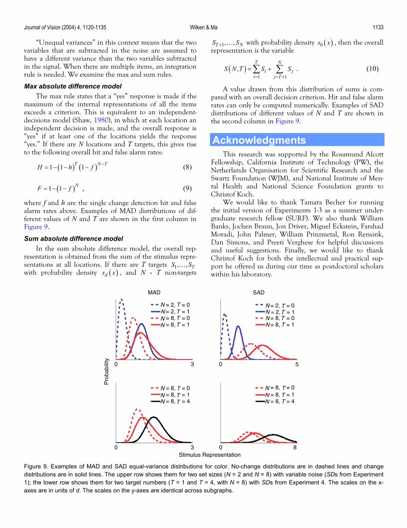
Max absolute difference model The max rule states that a “yes” response is made if the

maximum of the internal representations of all the

decisions model (Shaw, 1980), in wpendent decision is made, and the overall response is

“yes” if at least one of the locations yields the response “yes.” If there are N locations and T targets, this gives rise to the following overall hit and false alarm rates:

( ) ( )1 1 1T N TH h f −= − − − (8)

( )N1 1F f

f and h are the single

= − − , (9)

where alarm rates above. Examples of MAD distributions of dif-

and T are shown in the first colum Figure 9

is obtained from the sum of the stimulus repre-sentations at all locations. If there are T targets 1, , TS S…

with probability density ( )d

change detection hit and false Chr

ferent values of N.

n in

Sum absolute difference model In the sum absolute difference model, the overall rep-

resentation

s x , and N - T non-targets

( )01, ,T NS S+ … with probability density s x , then the overall repr

tri of supared with an overall decision criterion. Hit and false alarm rates be computed numerically. Examples of SAD distr

.

esentation is the variable

( )1 1

,T N

i ji j T

S N T S S= = +

= +∑ ∑ .

A value drawn from this

(10)

ms is com-dis bution

can only ibutions of different val

the second column in Figure 9ues of N and T are shown in

Acknowledgments This research was supported by the Rosamund Alcott

Fellowship, California Institute of Technology (PW), the Netherlands Organisation for Scientific Research and the

ational Institute of Men- Foundation grants to

almer, William Prinzmetal, Ron Rensink, Dan

within his laboratory.

Swartz Foundation (WJM), and Ntal Health and National Science

istof Koch. We would like to thank Tamara Becher for running

the initial version of Experiments 1-3 as a summer under-graduate research fellow (SURF). We also thank William Banks, Jochen Braun, Jon Driver, Miguel Eckstein, Farshad Moradi, John P

Simons, and Preeti Verghese for helpful discussions and useful suggestions. Finally, we would like to thank Christof Koch for both the intellectual and practical sup-port he offered us during our time as postdoctoral scholars

0 3

Pro

babi

lity

MAD

= 2, = 0 = 2, = 1 = 8, = 0 = 8, = 1

0 5

SAD

= 2, = 0 = 2, = 1

= 8, = 0 = 8, = 1

0 3Stimulus Representation

= 8, = 0 = 8, = 1 = 8, = 4

0 8

= 8, = 0 = 8, = 1 = 8, = 4

N

NN

NN

NN

N

NN

NNN

NTT

TTT

T

TT

TTT

T

T T

Figure 9. Examples of MAD and SAD equal-variance distributions for color. No-change distributions are in dashed lines and changedistributions are in solid lines. The upper row shows them for two set sizes (N = 2 and N = 8) with variable noise (SDs from Experiment1); the lower row shows them for two target numbers (T = 1 and T = 4, with N = 8) with SDs from Experiment 4. The scales on the x-axes are in units of d. The scales on the y-axes are identical across subgraphs.

Journal of Vision (2004) 4, 1120-1135 Wilken & Ma 1134

Commercial relationships: none. Corresponding author: Patrick Wilken. Email: patrick.wilken@nat.uni-magdeburg.de. Address: Otto von Guericke Universität, Fakultät für Naturwissenschaften, Universitätplatz 2, D-39106 Magde-burg, Germany.

References Abramowitz, M., & Stegun, I. A. (1965). Handbook of

mathematical functions, with formulas, graphs, and mathe-matical tables. New York: Dover Publications.

nagh, P. (2004). The capacity of vis-emory is set both by visual informa-

tion load and by number of objects. Psychological Sci-

Brain x. Spatial Vision, 10, 433-436. [PubMed]

Brau

Cow mber 4 in short-term

(1), 87-114. [PubMed]

effects of set size on visual search accuracy for feature, con-

Georgeson, M. A. (1991). Contrast overconstancy. Journal

Geor

quency channels. Journal of Physiology, 252(3), 627-656.

Gree Swets, J. A. (1966). Signal detection theory and psychophysics. New York: Wiley.

Gree

Kana erstraten, F. A. J. (2004). Visual transients

(19), 2233-2240. [PubMed]

Luck city of visual working memory for features and conjunctions. Na-

Macer's guide. New York: Cambridge University

Press.

Mag(6), 247-251. [PubMed]

y. Journal of Experimental Psychology: Learning,

Mag

Mag psycho-

Mag pat-

Mag & Dyrnes,

Magnussen, S., Greenlee, M. W., & Thomas, J. P. (1996).

Mard Statistics of directional data. London:

Olso

64(7), 1055-1067.

Palm ntional limits on the perception and

Palm ). Attention in visual search: Distinguishing

Palmarch. Vision Research, 40(10-12),

Pashl69-378. [PubMed]

42. [PubMed]

-

Alvarez, G. A., & Cavaual short-term m

ence, 15(2), 106-111. [PubMed]

ard, D. H. (1997). The Psychophysics Toolbo

n, J., Koch, C., & Davis, J. L. (2001). Visual attention and cortical circuits. Cambridge, MA: MIT Press.

an, N. (2001). The m nuagical memory: A reconsideration of mental storage capacity. Behavioral and Brain Sciences, 24

Eckstein, M. P., Thomas, J. P., Palmer, J., & Shimozaki, S. S. (2000). A signal detection model predicts the

junction, triple conjunction, and disjunction displays. Perception & Psychophysics, 62(3), 425-451. [PubMed]

of the Optical Society of America A, 8(3), 579-586. [PubMed]

geson, M. A., & Sullivan, G. D. (1975). Contrast con-stancy: Deblurring in human vision by fre- spatial

[PubMed]

n , &, D. M.

n, D. M., & Swets, J. A. (1978). Detection and recog-nition. Psychological Review, 85, 192-206.

i, V R., & without feature changes are sufficient for the percept of a change. Vision Research, 44

, S. J., & Vogel, E. K. (1997). The capa

ture, 390, 279-281. [PubMed]

millan, N. A., & Creelman, C. D. (1991). Detection t usheory: A

nussen, S. (2000). Low-level memory processes in vi-sion. Trends in Neuro 23

Magnussen, S., & Greenlee, M. W. (1992). Retention and disruption of motion information in visual short-term memorMemory, and Cognition, 18, 151-156. [PubMed]

nussen, S., & Greenlee, M. W. (1997). Co n mpetitioand sharing of processing resources in visual discrimi-nation. Journal of Experimental Psychology: Human Percep-tion and Performance, 23(6), 1603-1616. [PubMed]

nussen, S., & Greenlee, M. W. (19 e 99). Thphysics of perceptual memory. Psychological Research, 62(2-3), 81-92. [PubMed]

nussen, S., Greenlee, M. W., Asplund, R., & Dyrnes, S. (1990). Perfect short-term memory fo icr periodterns. European Journal of Cognitive Psychology, 2, 245-262.

nussen, S., Gree . W., Asplund, R., nlee, MS. (1991). Stimulus-specific mechanisms of visual short-term memory. Vision Research, 31(7-8), 1213-1219. [PubMed]

Parallel processing in visual short-term memory. Jour-nal of Experimental Psychology: Human Perception and Per-formance, 22(1), 202-212. [PubMed]

ia, K. ).V. (1972Academic Press.

n, I. R., & Jiang, Y. (2002). Is visual short-term mem-ory object based? Rejection of the “strong-object” hy-pothesis. Perception & Psy s, chophysic[PubMed]

er, J. (1990). Attememory of visual information. Journal of Experimental Psychology: Human Perception and Performance, 16(2), 332-350. [PubMed]

e 5r, J. (199four causes of a set-size effect. Current Directions in Psy-chological Science, 4(4), 118-123.

er, J., Verghese, P., & Pavel, M. (2000). The psycho-physics o sef visual 1227-1268. [PubMed]

er, H. (1988). Familiarity and visual change detection. Perception & Psychophysics, 44(4), 3

Pelli, D. G. (1997). The VideoToolbox software for visual psychophysics: Transforming numbers into movies. Spatial Vision -4, 10, 437

Prinzmetal, W., Amiri, H., Allen, K., & Edwards, T. (1998). Phenomenology of attention. 1. C locaolour, tion, orientation and spatial frequency. Journal of Ex-perimental Psychology: Human Perception and Performance, 24, 261-282.

sciences,

Journal of Vision (2004) 4, 1120-1135 Wilken & Ma 1135

Prinzmetal, W., Nwachuku, I., Bodanski, L., Blumenfeld, L., & Shimizu, N. (1997). The phenomenology of at-tention. 2. Brightness and contrast. Consciousness & Cognition, 6(2-3), 372-412. [PubMed]

nouille, M. (19Que 49). Approximate tests of correlation in

Rega Journal of the Op-

Rens of attentional processing. Visual Cogni-

Roseal results and

(4), 985-999. [PubMed]

Shaw s of in-

Swet

ed]

time series. Journal of the Royal Statistical Society (Series B), 11, 68-84.

n, D. (1985). Storage of spatial-frequency information and spatial-frequency discri n.minatio

le sourc

PubMed

PubMed

PubMed

-76. [Pub

PubMed

Wright, M.J., Alston, L., & Popple, A.V. (2002). Set-size effects for spatial frequency change and discrimination in multiple targets. Spatial Vision, 15(2), 157-170. [PubMed]

tical Society of America A, 2(4), 619-621.

ink, R. A. (2000). Visual search for change: A probe into the naturetion, 7(1-3), 345-376.

nholtz, R. (2001). Visual search for orientation among heterogeneous distractors: Experimentimplications for signal-detection theory models of search. Journal of Experimental Psychology: Human Percep-tion and Performance, 27

Shaw, M. L. (1980). Identifying attentional and decision-making components in information processing. In R. S. Nickerson (Ed.), Attention and Performance VIII (pp. 277-295). Hillsdale, NJ: Lawrence Erlbaum Associated.

, M. L. (1982). Attending to multip eformation. Cognitive Psychology, 14, 353-409.

s, J. A. (1986a). Form of empirical ROCs in discrimi-nation and diagnostic tasks: Implications for theory and measurement of performance. Psychological Bulle-tin, 99(2), 181-198. [PubMed]

Swets, J. A. (1986b). Indices of discrimination or diagnostic accuracy: Their ROCs and implied models. Psychologi-cal Bulletin, 99(1), 100-117. [ ]

Tukey, J. W. (1958). Bias and confidence in not quite large samples. Annals of Mathematical Statistics, 29, 614.

Verghese, P. (2001). Visual search and attention: A signal detection theory approach. Neuron, 31(4), 523-535. [ ]

Vogel, E.K., Woodman, G.F., & Luck, S.J. (2001). Storage of features, conjunctions and objects in visual working memory. Journal of Experimental Psychology: Human Per-ception and Performance, 27, 92-114. [ ]

Wickens, T.D. (2002). Elementary signal detection theory. Ox-ford ; New York: Oxford University Press.

Wilken, P. (2001). Capacity limits for the detection and identi-fication of change: Implications for models of visual short-term memory. Unpublished doctoral dissertation, Uni-versity of Melbourne, Melbourne.

Wolfe, J.M. (2003). Moving towards solutions to some enduring controversies in visual search. Trends in Cognitive Sciences, 7(2), 70 M

Woodman, G.F., Vogel, E.K., & Luck, S.J. (2001). Visual search remains efficient when visual working memory is full. Psychological Science, 12(3), 219-224. [ ]