a deep learning approach to species distribution modelling
TRANSCRIPT

HAL Id hal-01834227httpshalarchives-ouvertesfrhal-01834227
Submitted on 10 Jul 2018
HAL is a multi-disciplinary open accessarchive for the deposit and dissemination of sci-entific research documents whether they are pub-lished or not The documents may come fromteaching and research institutions in France orabroad or from public or private research centers
Lrsquoarchive ouverte pluridisciplinaire HAL estdestineacutee au deacutepocirct et agrave la diffusion de documentsscientifiques de niveau recherche publieacutes ou noneacutemanant des eacutetablissements drsquoenseignement et derecherche franccedilais ou eacutetrangers des laboratoirespublics ou priveacutes
A deep learning approach to Species DistributionModelling
Christophe Botella Alexis Joly Pierre Bonnet Pascal Monestiez FranccediloisMunoz
To cite this versionChristophe Botella Alexis Joly Pierre Bonnet Pascal Monestiez Franccedilois Munoz A deep learningapproach to Species Distribution Modelling Alexis Joly Stefanos Vrochidis Kostas Karatzas AriKarppinen Pierre Bonnet Multimedia Tools and Applications for Environmental amp Biodiversity In-formatics Springer pp169-199 2018 Multimedia Systems and Applications Series 978-3-319-76444-3 101007978-3-319-76445-0_10 hal-01834227
[Preprint]A deep learning approach to Species Distribution Modelling
Christophe Botella1235 Alexis Joly1 Pierre Bonnet34 Pascal Monestiez5 and FranccediloisMunoz6
1INRIA Sophia-Antipolis - ZENITH team LIRMM - UMR 5506 - CC 477 161 rue Ada34095 Montpellier Cedex 5 France
2INRA UMR AMAP F-34398 Montpellier France3AMAP Univ Montpellier CIRAD CNRS INRA IRD Montpellier France
4CIRAD UMR AMAP F-34398 Montpellier France5BioSP INRA Site Agroparc 84914 Avignon France
6Universiteacute Grenoble Alpes 621 avenue Centrale 38400 Saint-Martin-drsquoHegraveres France
December 1 2017
Accepted in Multimedia Tools and ApplicationsTitle of Book Multimedia Technologies for Environmental amp Biodiversity Informatics
Abstract
Species distribution models (SDM) are widely used for ecological research and conservationpurposes Given a set of species occurrence the aim is to infer its spatial distribution over a giventerritory Because of the limited number of occurrences of specimens this is usually achievedthrough environmental niche modeling approaches ie by predicting the distribution in thegeographic space on the basis of a mathematical representation of their known distribution inenvironmental space (= realized ecological niche) The environment is in most cases representedby climate data (such as temperature and precipitation) but other variables such as soil type orland cover can also be used In this paper we propose a deep learning approach to the problem inorder to improve the predictive effectiveness Non-linear prediction models have been of interest forSDM for more than a decade but our study is the first one bringing empirical evidence that deepconvolutional and multilabel models might participate to resolve the limitations of SDM Indeedthe main challenge is that the realized ecological niche is often very different from the theoreticalfundamental niche due to environment perturbation history species propagation constraints andbiotic interactions Thus the realized abundance in the environmental feature space can have avery irregular shape that can be difficult to capture with classical models Deep neural networkson the other side have been shown to be able to learn complex non-linear transformations ina wide variety of domains Moreover spatial patterns in environmental variables often containsuseful information for species distribution but are usually not considered in classical models Ourstudy shows empirically how convolutional neural networks efficiently use this information andimprove prediction performance
1 Introduction
11 Context on species distribution models
Species distribution models (SDM) have become increasingly important in the last few decades for thestudy of biodiversity macro ecology community ecology and the ecology of conservation An accurate
1
knowledge of the spatial distribution of species is actually of crucial importance for many concrete sce-narios including the landscape management the preservation of rare andor endangered species thesurveillance of alien invasive species the measurement of human impact or climate change on speciesetc Concretely the goal of SDM is to infer the spatial distribution of a given species based on a setof geo-localized occurrences of that species (collected by naturalists field ecologists nature observerscitizen sciences project etc) However it is usually not possible to learn that distribution directlyfrom the spatial positions of the input occurrences The two major problems are the limited numberof occurrences and the bias of the sampling effort compared to the real underlying distribution In areal-world dataset the raw spatial distribution of the observations is actually highly correlated to thepreference and habits of the observers and not only to the spatial distribution of the species Anotherdifficulty is that in most cases we only have access to presence data but not to absence data Inother words occurrences inform that a species was observed at a given location but never that it wasnot observed at a given location Consequently a region without any observed specimen in the dataremains highly uncertain Some specimens could live there but were not observed or no specimenlive there but this information is not recorded Finally knowing abundance in space doesnrsquot giveinformation about the ecological determinants of species presenceFor all these reasons SDM is usually achieved through environmental niche modeling approachesie by predicting the distribution in the geographic space on the basis of a representation in theenvironmental space This environmental space is in most cases represented by climate data (suchas temperature and precipitation) but also by other variables such as soil type land cover distanceto water etc Then the objective is to learn a function that takes the environmental feature vectorof a given location as input and outputs an estimate of the abundance of the species The mainunderlying hypothesis is that the abundance function is related to the fundamental ecological nicheof the species in the sense of Hutchinson (see Hutchinson [1957]) That means that in theory agiven species is likely to live in a single privileged ecological niche characterized by an unimodaldistribution in the environmental space However in reality the abundance function is expected tobe more complex Many phenomena can actually affect the distribution of the species relative to itsso called abiotic preferences For instance environment perturbations or geographical constraints orinteractions with other living organisms (including humans) might have encourage specimens of thatspecies to live in a different environment As a consequence the realized ecological niche of a speciescan be much more diverse and complex than its hypothetical fundamental niche
12 Interest of deep and convolutional neural networks for SDM
Notations When talking about environmental input data there could be confusions between theirdifferent possible formats Without precisions given x will represent a general input environmentalvariable which can have any format When a distinction is made x will represent a vector while anarray is always noted X To avoid confusions on notations for the differents index kinds we note thespatial site index as superscript on the input variable (xk or Xk for kth site) and the component indexas subscript (so xkj for the jth component of kth site vector xk isin Rp or for the array Xk isinMdep(R)Xkj is the j
th matrix slice taken on its second dimension) When we denote an input associated witha precise point location taken in a continuous spatial domain the point z is noted as argument x(z)
Classical SDM approaches postulate that the relationship between output and environmentalvariables is relatively simple typically of the form
g(E[y|x]) =sumj
fj(xj) +sumjjprime
hjjprime(xj xjprime) (1)
where y is the response variable targeted a presence indicator or an abundance in our case thexj rsquos are components of a vector of environmental variables given as input for our model fj are real
2
monovariate functions of it hjjprime are bivariate real functions representing pairwise interactions effectsbetween inputs and g is a link function that makes sure E[y|x] lies in the space of our responsevariable y State-of-the-art classification or regression models used for SDM in this way include GAM(Hastie amp Tibshirani [1986]) MARS (Friedman [1991]) or MAXENT (Phillips et al [2004]Phillipset al [2006]) Thanks to fj we can isolate and understand the effect of the environmental factor xjon the response Often pairwise effects form of hjjprime is restricted to products like it is the case inthe very popular model MAXENT It facilitates the interpretation and limits the dimensionality ofmodel parameters However it sets a strong prior constraint without a clear theoretical founding asthe explanatory factors of a species presence can be related to complex environmental patternsTo overcome this limitation deep feedforward neural networks (NN) (Goodfellow et al [2016]) aregood candidates because their architecture favor high order interactions effects between the inputvariables without constraining too much their functional form thanks to the depth of their architec-ture To date deep NN have shown very successful applications in particular image classification(Krizhevsky et al [2012]) Until now to our knowledge only one-layered-NNrsquos have been testedin the context of SDM (eg in Lek et al [1996] or Thuiller [2003]) If they are able to capture alarge panel of multivariate functions when they have a large number of neurons their optimizationis difficult and deep NN have been shown empirically to improve optimization and performance (seesection 641 in Goodfellow et al [2016]) However NN overfit seriously when dealing with smalldatasets which is the case here (asymp 5000 data) for this reason we need to find a way to regularizethose models in a relevant way An idea that is often used in SDM (see for example Leathwick et al[2006]) and beyond is to mutualize the heavy parametric part of the model for many species responsesin order to reduce the space of parameters with highest likelihood To put it another way a NN thatshares last hidden layer neurons for the responses of many species imposes a clear constraint theparameters must construct high level ecological concepts which will explain as much as possible theabundance of all species These high-level descriptors whose number is controlled should be seen asenvironmental variables that synthesize the most relevant information in the initial variablesAnother limitation of models described by equation (1) is that they donrsquot capture spatial autocor-relation of species distribution nor the information of spatial patterns described by environmentalvariables which can impact species presence In the case of image recognition where the explanatorydata is an image the variables the pixels are spatially correlated as are the environmental variablesused in the species distribution models Moreover the different channels of an image RGB can notbe considered as being independent of the others because they are conditioned by the nature of thephotographed object We can see the environmental variables of a natural landscape in the same wayas the channels of an image noting that climatic soil topological or land use factors have strongcorrelations with others they are basically not independent of each other Some can be explained bycommon mechanisms as is the case with the different climatic variables but some also act directly onothers as is the case for soil and climatic conditions on land use in agriculture or the topology on theclimate These different descriptors can be linked by the concept of ecological environment Thusthe heuristic that guides our approach is that the ecological niche of a species can be more effectivelyassociated with high level ecological descriptors that combine non linearly the environmental variableson one hand and the identification of multidimensional spatial patterns of images of environmentaldescriptors on the other hand Convolutional neural networks (CNN see LeCun et al [1989]) appliedto multi-dimensional spatial rasters of environmental variables can theoretically capture those whichmakes them of particular interest
13 Contribution
This work is the first attempt in applying deep feedforward neural networks and convolutional neuralnetworks in particular to species distribution modeling It introduces and evaluates several architec-tures based on a probabilistic modeling suited for regression on count data the Poisson regressionIndeed species occurrences are often spatially degraded in publicly available datasets so that it isstatistically and computationally more relevant to aggregate them into counts In particular our
3
experiments are based on the count data of the National Inventory for Nature Protection (INPN1)for 50 plant species over the metropolitan French territory along with various environmental dataOur models are compared to MAXENT which is among the most used classical model in ecologyOur results first show how mutualizing model features for many species prevent deep NN to overfitand finally allow them to reach a better predictive performance than the MAXENT baseline Thenour results show that convolutional neural networks performed even better than classical deep feed-forward networks This shows that spatially extended environmental patterns contain relevant extrainformation compared to their punctual values and that species generally have a highly autocorre-lated distribution in space Overall an important outcome of our study is to show that a restrictednumber of adequately transformed environmental variables can be used to predict the distribution ofa huge number of species We believe the study of the high-level environmental descriptors learnedby the deep NNs could help to better understand the co-abundance of different species and wouldbe of great interest for ecologists
2 A Deep learning model for SDM
21 A large-scale Poisson count model
In this part we introduce the statistical model which we assume generates the observed data Ourdata are species observations without sampling protocol and spatially aggregated on large spatialquadrat cells of 10x10km Thus it is relevant to see them as counts
To introduce our proposed model we first need to clarify the distinction between the notion ofobsvered abundance and probability of presence Abundance is a number of specimens relativelyto an area In this work we model species observed abundance rather than probability of presencebecause we work with presence only data and without any information about the sampling processUsing presence-absence models such as logistic regression could be possible but it would require toarbitrarily generate absence data And it has been shown that doing so can highly affect estimationand give biased estimates of total population Ward et al [2009] Working with observed abundancedoesnrsquot bias the estimation as long as the space if homogeneously observed and we donrsquot look forabsolute abundance but rather relative abundance in spaceThe observed abundance ie the number of specimens of a plant species found in a spatial area isvery often modeled by a Poisson distribution in ecology when a large number of seeds are spreadin the domain each being independent and having the same probability of growing and being seenby someone the number of observed specimens in the domain will behave very closely to a Poissondistribution Furthermore many recent SDM models especially MAXENT as we will see later arebased on inhomogeneous Poisson point processes (IPP) to model the distribution of species specimensin an heterogeneous environment However when geolocated observations are aggregated in spatialquadrats (asymp 10km x 10km each in our case) observations must be interpreted as count per quadrats Ifwe considerK quadrats named (s1 sK) (we will call them sites from now) with empty intersectionand we consider observed specimens are distributed according to IPP(λ) where λ is a positivefunction defined on Rp and integrable over our study domain D (where x is known everywhere) weobtain the following equation
forallk isin [|1K|] N(sk) sim P(int
sk
λ(x(z))dz
)(2)
Now in a parametric context for the estimation of the parameters of λ we need to evaluate theintegral by computing a weighted sum of λ values taken at quadrature points representing all thepotential variation of λ As our variables x are constant by spatial patches we need to computeλ on every point with a unique value of x inside sk and to do this for every k isin [|1K|] Thiscan be very computationally and memory expensive For example if we take a point per square
1httphttpsinpnmnhnfr
4
km (common resolution for environmental variables) it would represent 518100 points of vector orpatch input to extract from environmental data and to handle in the learning process At the sametime environmental variables are very autocorrelated in space so the gain estimation quality canbe small compared to taking a single point per site Thus for simplicity we preferred to make theassumption albeit coarse that the environmental variables are constant on each site and we take thecentral point to represent it Under this assumption we justify by the following property the Poissonregression for estimating the intensity of an IPP
Property The inhomogeneous Poisson process estimate is equivalent to a Poisson regression esti-mate with the hypothesis that x(z) is constant over every site
Proof We note z1 zN isin D the N species observations points K the number of disjoints sitesmaking a partition of D and assumed to have an equal area We write the likelihood of z1 zNaccording to the inhomogeneous poisson process of intensity function λ isin (R+)D
p(z1 zN |λ) = p(N |λ)Nprodi=1
p(zi|λ)
=(intD λ)
N
N exp
(minusintDλ
) Nprodi=1
λ(x(zi))intD λ
=exp
(minusintD λ)
N
Nprodi=1
λ(x(zi))
We transform the likelihood with the logarithm for calculations commodity
log(p(z1 zN |λ)) =Nsumi=1
log (λ(x(zi)))minusintDλminus log(N )
We leave the N term as it has no impact on the optimisation of the likelihood with respect to theparameters of λ
Nsumi=1
log (λ(x(zi)))minusintDλ =
Nsumi=1
log (λ(x(zi)))minussum
kisinSites
|D|Kλ(xk)
=sum
kisinSites
nk log(λ(xk)
)minus |D|
Kλ(xk)
Where nk is the number of species occurrences that fall in site k We can aggregate the occurrencesthat are in a same site because x is the same for them We can now factorize |D|K on the wholesum which brings us up to the factor to the the poisson regression likelihood with pseudo-countsKnk|D|
=|D|D
sumkisinSites
Dnk|D|
log(λ(xk)
)minus λ(xk)
So maximizing this log-likelihood is exactly equivalent to maximizing the initial Poisson process like-lihood
Proof uses the re-expression of the IPP likelihood inspired from Berman amp Turner [1992] as that ofthe associated Poisson regression In the following parts we always consider that for a given speciesthe number y of specimens observed in a site of environmental input x is as follows
5
y sim P(λmθ(x)) (3)
Where m is a model architecture with parameters θFrom equation (3) we can write the likelihood of counts on K different sites (x1 xK) for Nindependently distributed species with abundance functions (λmiθi)iisin[|1N |] isin (R+)R
p respectivelydetermined by models (mi)iisin[|1N |] and parameters (θi)iisin[|1N |]
p((yik)iisin[|1N |]kisin[|1K|]|(λmiθi)iisin[|1N |]
)=
Nprodi=1
Kprodk=1
(λmiθi(xk))yik
yikexp(minusλmiθi(xk))
Which gives when eliminating log(yik) terms (which are constant relatively to models parameters)the following negative log-likelihood
L((yik)iisin[|1N |]kisin[|1K|]|(λmiθi)iisin[|1N |]
)=
Nsumi=1
Ksumk=1
λmiθi(xk)minus yik log(λmiθi(xk)) (4)
Following the principle of maximum likelihood for fitting a model architecture we minimize theobjective function given in equation (4) relatively to parameters θ
22 Links with MAXENT
For our experiment we want to compare our proposed models to a state of the art method commonlyused in ecology We explain in the following why and how we can compare the chosen referenceMAXENT with our models
MAXENT (Phillips et al [2004]Phillips et al [2006]) is a popular SDM method and relatedsoftware for estimating relative abundance as a function of environmental variables from presenceonly data points This method has proved to be one of the most efficient in prediction P Andersonet al [2006] while guaranteeing a good interpretability thanks to the simple elementary form of itsfeatures and its variable selection procedure The form of the relative abundance function belongs tothe class described in Equation 1 More specifically
log (λMAXθ(x)) = α+
psumj=1
Ssums=1
fsj (x(j)) +sumjltjprime
βjjprimexjxprimej (5)
where x(j) is the jth component of vector x The link function is a logarithm and variablesinteractions effects are product interactions If xj is a quantitative variable the functions (fs)sisin[|1S|]belongs to 4 categories linear quadratic threshold and hinge One can get details on the hingesfunctions used in MAXENT in Phillips amp Dudiacutek [2008] If xj is categorical then fj takes a differentvalue for every category with one zero categoryIt has been shown that MAXENT method is equivalent to the estimation of an IPP intensity functionwith a specific form and a weighted L1 penalty on its variables Fithian amp Hastie [2013] Letrsquos callλMAXθ(x) the intensity predicted by MAXENT with parameters θ at x Last property says thaton any given dataset θ estimated from a Poisson regression (aggregating observations as counts persite) is the same as the one of the IPP (each observation is an individual point even when there areseveral at a same site) In our experiments we ran MAXENT using the maxnet package in R Phillipset al [2017] with the default regularization and giving to the function
1 A positive point per observation of the species
2 A pseudo-absence point per site
6
MAXENT returns only the parameters of the (fsj )sj and the (βjjprime)jltjprime but not the interceptα as it is meant to only estimate the absolute abundance We donrsquot aim at estimating absoluteabundance either however we need the intercept to measure interesting performance metrics acrossall the compared models To resolve this for each species we fitted the following model using theglm package in R as a second step
y sim P (exp(α+ log(p)))
Where α is our targeted intercept p is the relative intensity prediction given by MAXENT at thegiven site and y is the observed number of specimens at this site
23 SDM based on a fully-connected NN model
We give in the following a brief description of the general structure of fully-connected NN modelsand how we decline it in our tested deep model architecture
General introduction of fully-connected NN models A deep NN is a multi-layered modelable to learn complex non-linear relationship between an input data which in our case will be avector x isin Rp of environmental variables that is assumed to represent a spatial site and outputvariables y1 yN which in our case is species counts in the spatial site The classic so called fully-connected NN model is composed of one or more hidden layer(s) and each layer is composedof one or more neuron(s) We note n(lm) the number of neurons of layer l in model architecturem m parameters are stored in θ In the first layer each neuron is the result of a parametric linearcombination of the elements of x which is then transformed by an activation function a So for aNN m a1jm (x θ) = a(xT θ1j ) is called the activation of jth neuron of the first hidden layer of m whenit is applied to x Thus on the lth layer with l gt 1 the activation of the jth neuron is a((θlj)
Talminus1m )Now we understand that the neuron is the unit that potentially combines every variables in x andits activation inducing a non-linearity to the parametric combination it can be understood as a par-ticular basis function in the p dimensional space of x Thus the model is able to combine as manybasis functions as there are neurons in each layer and the basis functions become more and morecomplex when going to further layers Finally these operations makes m theoretically able to closelyfit a broad range of functions of xLearning of model parameters is done through optimization (minimization by convention) of an ob-jective function that depends on the prediction goal Optimization method for NN parameters θ isbased on stochastic gradient descent algorithms however the loss function gradient is approximatedby the back-propagation algorithm Rumelhart et al [1988]Learning a NN model lead to a lot of technical difficulties that have been progressively dealt withduring last decade and through many different techniques We present some that have been of par-ticular interest in our study A first point is that there are several types of activation functions thefirst one introduced being the sigmoid function However the extinction of its gradient when xT θ1j issmall or big has presented a serious problem for parameters optimization in the past More recentlythe introduction of the ReLU (Nair amp Hinton [2010]) activation function helped made an importantstep forward in NNs optimization A second point is that when we train a NN model simultaneouschanges of all the parameters lead to important change in the distribution (across the dataset) of eachactivation of the model This phenomenon is called internal covariate shift and perturbs learningimportantly Batch-Normalization (Ioffe amp Szegedy [2015]) is a technique that significantly reducesinternal covariate shift and help to regularize our model as well It consists of a parameterized cen-tering and reduction of pre-activations This facilitates optimization and enables to raise the learningrate leading to a quicker convergence At the same time it has a regularization effect because thecentering and reduction of a neuron activation is linked to the mini-batch statistics The mini-batchselection being stochastic at every iteration a neuron activation is stochastic itself and the model
7
will not rely on it when it has no good effect on prediction
Models architecture in this study For a given species i When we know the model parameterθ we can predict the parameter of the Poisson distribution of the random response variable yi isin Nie the count of species i conditionally on its corresponding input x with the formula
λmθ(x) = exp(γTi aNhm (x θ)) (6)
For this work we chose the logarithm as link function g mentioned in 12 It is the conventional linkfunction for the generalized linear model with Poisson family law and is coherent with MAXENTγi isin Rn(Nhm) is included in θ It does the linear combinations of last layer neurons activations for thespecific response i If we set n(Nhm) = 200 as we do in the following experiments there are only 200parameters to learn per individual species while there are a lot more in the shared part of the modelthat builds aNh
m (x θ) Now for model fitting we follow the method of the maximum likelihood theobjective function will be a negative-loglikelihood but it could otherwise be some other predictionerror function Note that we will rather use the term loss function than negative loglikelihood forsimplicity We chose the ReLU as activation function because it showed empirically less opti-mization problems and a quicker convergence Plus we empirically noticed the gain in optimizationspeed and less complications with the learning rate initialization when using Batch-NormalizationFor this reason Batch-Normalization is applied to every pre-activation (before applying the ReLU)to every class of NN model in this paper even with CNNs We give a general representation of theclass of NN models used in this work in Figure 1
Figure 1 A schematic representation of fully-connected NN architecture Except writings imagecomes from MichaelregNielsen3
24 SDM based on a convolutional NN model
A convolutional NN (CNN) can be seen as a extension of NN that are particularly suited to deal withcertain kind of input data with very large dimensions They are of particular interest in modelingspecies distribution because they are able to capture the effect of spatial environmental patternsAgain we will firstly describe the general form of CNN before going to our modeling choices
General introduction of CNN models CNN is a form of neural network introduced in LeCunet al [1989] It aims to efficiently apply NN to input data of large size (typically 2D or 3D arrayslike images) where elements are spatially auto-correlated For example using a fully-connected neural
8
network with 200 neurons on an input RGB image of dimensions 256x256x3 would imply around4 lowast 107 parameters only for the first layer which is already too heavy computationally to optimizeon a standard computer these days Rather than applying a weight to every pixel of an input arrayCNN will apply a parametric discrete convolution based on a kernel of reasonable size ( 33por 55p are common for NNp input arrays) on the input arrays to get an intermediate featuremap (2D) The convolution is applied with a moving windows as illustrated in Figure 2 -B NotingX isin Mddp an input array we simplify notations in all that follows by writing CV(X kγ(c)) theresulting feature map from applying the convolution with (c c p) kernel of parameters γ isin Rc2p Ifthe convolution is applied directly on X the sliding window will pass its center over every Xij fromthe up-left to the bottom-right corner and produce a feature map with a smaller size than the inputbecause c gt 1 The zero-padding operation removes this effect by adding (cminus 1)2 layers of 0 onevery side of the array After a convolution there can be a Batch-Normalization and an activationfunction is generally applied to each pixel of the features maps Then there is a synthesizing stepmade by the pooling operation Pooling aggregates groups of cells in a feature map in order to reduceits size and introduce invariance to local translations and distortions After having composed theseoperations several times when the size of feature maps is reasonably small (typically reaching 1 pixel)a flattening operation is applied to transform the 3D array containing all the feature maps into avector This features vector will then be given as input to a fully-connected layer as we described inlast part The global concept underlying convolution layers operations is that first layers act as lowlevel interpretations of the signal leading to activations for salient or textural patterns Last layerson their side are able to detect more complex patterns like eyes or ears in the case of a face pictureThose high levels features have much greater sense regarding predictions we want to make Plus theyare of much smaller dimension than the input data which is more manageable for a fully-connectedlayer
Constitution of a CNN model for SDM The idea which pushes the use of CNN models forSDM is that complex spatial patterns like a water network a valley etc can affect importantly thespecies abundance This kind of pattern canrsquot be really deducted for punctual values of environmentalvariables Thus we have chosen to build a SDM model which takes as input an array with a mapof values for each environmental variable that is used in the other models This way we will beable to conclude if there is extra relevant information in environmental variables spatial patterns topredict better species distribution In 2 -A we show for a single site a subsample of environmentalvariables maps taken as input by our CNN model To provide some more detail about the modelarchitecture the input array X is systematically padded such that the feature map resulting fromthe convolution is of same size as 2 first dimensions of the input ((c minus 1)2 cells of 0 after on thesides of the 2 dimensions) To illustrate that our padding policy is the same as the one illustratedin the example given in Figure 2 -B However notice that the kernel size can differ and the thirddimension size of input array will be the number of input variables or feature maps For an exampleof For the reasons described in 23 we applied a Batch-Normalization to each feature map(same normalization for every pixels of a map) before the activation which is still a ReLU For thepooling opreation we chose the average pooling which seems intuitively more relevant to evaluatean abundance (=concentration) The different kinds of operations and their succession in our CNNmodel are illustrated in the Figure 2 -C
3 Data and methods
31 Observations data of INPN
This paper is based on a reference dataset composed of count data collected and validated by Frenchexpert naturalists This dataset referred as INPN4 for national inventory of natural heritage
4httpsinpnmnhnfr
9
Figure 2 (a) Examples of input environmental data (b) for convolution pooling and flattening processin our (c) Convolutional Neural Network architecture
Dutregraveve B [2016] comes from the GBIF portal5 It provides access to occurrences data collectedin various contexts including Flora and regional catalogs specific inventories field note books andprospections carried out by the botanical conservatories In total the INPN data available on theGBIF contains 20999334 occurrences covering 7626 species from which we selected 1000 speciesThe assets of this data are the quality of their taxonomic identification (provided by an expertnetwork) their volume and geographic coverage Its main limitation however is that the geolocationof the occurrences was degraded (for plant protection concerns) More precisely all geolocations were
5httpswwwgbiforg
10
aggregated to the closest central point of a spatial grid composed of 100 km2 quadrat cells (ie sitesof 10times10km) Thus the number of observations of a species falling in a site gives a countIn total our study is based on 5181 sites which are split in 4781 training sites for fitting modelsand 400 test sites for validating and comparing models predictions
32 Species selection
For the genericity of our results and to make sure they are not biased by the choice of a particularcategory of species we have chosen to work with a high number of randomly chosen species Fromthe 7626 initial species we selected species with more than 300 observations We selected amongstthose a random subset of 1000 species to constitute an ensemble E1000 Then we randomly selected200 species amongst E1000 to constitute E200 and finally randomly selected 50 in E200 which gaveE50 E50 being the main dataset used to compare our model to the baselines we provide in Figure 1the list of species composing it The full dataset with species of E1000 contains 6134016 observationsin total (see Table 1 for the detailed informations per species)
33 Environnemental data
In the following we denote by p the number of environmental descriptors For this study we gath-ered and compiled different sources of environmental data into p = 46 geographic rasters containingthe pixel values of environmental descriptors presented in the table 2 with several resolutions na-ture of values but having a common cover all over the metropolitan French territory We chosesome typical environmental descriptors for modeling plant distribution that we believe carry relevantinformation both as punctual and spatial representation They can be classified as bioclimatic topo-logical pedologic hydrographic and land cover descriptors In the following we briefly describe thesources production method and resolution of initial data and the contingent specific post-processfor reproducibility
331 Climatic descriptors Chelsea Climate data 11
Those are raster data with worldwide coverage and 1km resolution A mechanistical climatic modelis used to make spatial predictions of monthly mean-max-min temperatures mean precipitations and19 bioclimatic variables which are downscaled with statistical models integrating historical measuresof meteorologic stations from 1979 to today The exact method is explained in the reference papersKarger et al [2016b] and Karger et al [2016a] The data is under Creative Commons Attribution40 International License and downloadable at (httpchelsa-climateorgdownloads)
332 Potential Evapotranspiration CGIAR-CSI ETP data
The CGIAR-CSI distributes this worldwide monthly potential-evapotranspiration raster data It ispulled from a model developed by Antonio Trabucco (Zomer et al [2007] Zomer et al [2008]) Thoseare estimated by the Hargreaves formula using mean monthly surface temperatures and standarddeviation from WorldClim 14 (httpwwwworldclimorgversion1) and radiation on top ofatmosphere The raster is at a 1km resolution and is freely downloadable for a nonprofit use athttpwwwcgiar-csiorgdataglobal-aridity-and-pet-databasedescription
333 Pedologic descriptors The ESDB v2 - 1kmx1km Raster Library
The library contains multiple soil pedology descriptor raster layers covering Eurasia at a resolutionof 1km We selected 11 descriptors from the library More precisely those variables have ordinalformat representing physico-chemical properties of the soil and come from the PTRDB The PTRDBvariables have been directly derived from the initial soil classification of the Soil Geographical DataBase of Europe (SGDBE) using expert rules SGDBE was a spatial relational data base relating spatial
11
Table 1 List of species in E50 with the total number of observations and prevalence in the fulldatabase
12
Name Description Nature Values ResolutionCHBIO_1 Annual Mean Temperature quanti [-106184] 30CHBIO_2 Mean of monthly max(temp)-min(temp) quanti [78210] 30CHBIO_3 Isothermality (100chbio_2chbio_7) quanti [412600] 30CHBIO_4 Temperature Seasonality (std dev100) quanti [302778] 30CHBIO_5 Max Temperature of Warmest Month quanti [36462] 30CHBIO_6 Min Temperature of Coldest Month quanti [-28253] 30CHBIO_7 Temp Annual Range (5- 6) quanti [167420] 30CHBIO_8 Mean Temp of Wettest Quarter quanti [-142230] 30CHBIO_9 Mean Temp of Driest Quarter quanti [-177265] 30CHBIO_10 Mean Temp of Warmest Quarter quanti [-28265] 30CHBIO_11 Mean Temp of Coldest Quarter quanti [-177118] 30CHBIO_12 Annual Precipitation quanti [3182543] 30CHBIO_13 Precip of Wettest Month quanti [4302855] 30CHBIO_14 Precip of Driest Month quanti [301356] 30CHBIO_15 Precip Seasonality (Coef of Var) quanti [82265] 30CHBIO_16 Precipitation of Wettest Quarter quanti [121855] 30CHBIO_17 Precipitation of Driest Quarter quanti [20421] 30CHBIO_18 Precip of Warmest Quarter quanti [1988517] 30CHBIO_19 Precip of Coldest Quarter quanti [6055204] 30etp Potential Evapo Transpiration quanti [1331176] 30alti Elevation quanti [-1884672] 3awc_top Topsoil available water capacity ordinal 0 120 165 21030bs_top Base saturation of the topsoil ordinal 35 62 85 30cec_top Topsoil cation exchange capacity ordinal 7 22 50 30crusting Soil crusting class ordinal [|0 5|]dgh Depth to a gleyed horizon ordinal 20 60 140 30dimp Depth to an impermeable layer ordinal 60 100 30erodi Soil erodibility class ordinal [|0 5|] 30oc_top Topsoil organic carbon content ordinal 1 2 4 8 30pd_top Topsoil packing density ordinal 1 2 30text Dominant surface textural class ordinal [|05|] 30proxi_eau lt50 meters to fresh water bool 0 1 30arti Artificial area clc isin 1 10 bool 0 1 30semi_arti Semi-artificial area clc isin 2 3 4 6 bool 0 1 30arable Arable land clc isin 21 22 bool 0 1 30pasture Pasture land clc isin 18 bool 0 1 30brl_for Broad-leaved forest clc isin 23 bool 0 1 30coni_for Coniferous forest clc isin 24 bool 0 1 30mixed_for Mixed forest clc isin 25 bool 0 1 30nat_grass Natural grasslands clc isin 26 bool 0 1 30moors Moors clc isin 27 bool 0 1 30sclero Sclerophyllous vegetation clc isin 28 bool 0 1 30transi_wood Transitional woodland-shrub clc isin 29 bool 0 1 30no_veg No or few vegetation clc isin 31 32 bool 0 1 30coastal_area Coastal area clc isin 37 38 39 42 30 bool 0 1 30ocean Ocean surface clc isin 44 bool 0 1 30
Table 2 Table of 46 environmental variables used in this study
13
units to a diverse pedological attributes of categorical nature which is not useful for our purpose Formore details see Panagos [2006] Panagos et al [2012] and Van Liedekerke et al [2006] The datais maintained and distributed freely for scientific use by the European Soil Data Centre (ESDAC) athttpeusoilsjrceceuropaeucontenteuropean-soil-database-v2-raster
334 Altitude USGS Digital Elevation data
The Shuttle Radar Topography Mission achieved in 2010 by Endeavour shuttle managed to measuredigital elevation at 3 arc second resolution over most of the earth surface Raw measures have beenpost-processed by NASA and NGA in order to correct detection anomalies The data is availablefrom the US Geological Survey and downloadable on the Earthexplorer (httpsearthexplorerusgsgov) One can refer to httpsltacrusgsgovSRTMVF for more informations
335 Hydrographic descriptor BD Carthage v3
BD Carthage is a spatial relational database holding many informations on the structure and natureof the french metropolitan hydrological network For the purpose of plants ecological niche we focuson the geometric segments representing watercourses and polygons representing hydrographic freshsurfaces The data has been produced by the Institut National de lrsquoinformation Geacuteographique etforestiegravere (IGN) from an interpretation of the BD Ortho IGN It is maintained by the SANDREunder free license for non-profit use and downloadable at httpservicessandreeaufrancefrtelechargementgeoETHBDCarthageFX From this shapefile we derived a raster containing thebinary value of variable proxi_eau ie proximity to fresh water all over France We used qgisto rasterize to a 125 meters resolution with a buffer of 50 meters the shapefile COURS_D_EAUshpon one hand and the polygons of SURFACES_HYDROGRAPHIQUESshp with attribute NATURE=Eaudouce permanente on the other hand We then created the maximum raster of the previous ones(So the value of 1 correspond to an approximate distance of less than 50 meters to a watercourse orhydrographic surface of fresh water)
336 Land cover Corine Land Cover 2012 version 1851 122016
It is a raster layer describing soil occupation with 48 categories across Europe (25 countries) at aresolution of 100 meters This classification is the result of an interpretation process from earth surfacehigh resolution satellite images This data base of the European Union is freely accessible online for alluse at httplandcopernicuseupan-europeancorine-land-coverclc-2012 and commonlyused for the purpose of plant distribution modeling For a need of meaningfull variables at ourscale and reduced memory consumption we reduced the number of categories to 14 following mainlythe procedure of They eliminate some categories of few interest too rare or inaccurate and groupscategories that are associated with similar plant communities In addition we introduce a categorySemi artificial surfaces which regroups perturbed natural areas interesting for the study of alieninvasive species We keep the Corine Land Cover category called Sea and ocean that can be animportant contextual variable for the convolutional neural network model and The final categoriesgroups are detailed in the table 2 for each of the retain categories we created a raster of the sameresolution as the original one where the value 1 means the pixel belongs to the category or the valueis 0 otherwise
337 Environmental variables extraction and format
When creating the p global GeoTIIF rasters as the original coordinate system of the layer vary amongsources we change it if necessary to WGS84 using rgdal package on R which is the coordinatesystem INPN occurrences databases As explained previously for computational reasons consideringthe scale and simplicity we chose to represent each site by a single geographic point and chose thecenter of the site We are going to compare two types of models For a site k the first takes as input
14
a vector of p elements which values are those of the environmental variables taken at the geolocationof the center of the site k while the other takes p rasters of size (dd) cropped (with package raster)from the global raster of each environmental descriptors and centered at the center of k If we denotereslonj the spatial resolution in longitude of global raster of the jth environmental descriptor andreslatj its resolution in latitude the spatial extent of Xk
j is (dreslatjtimesdreslonj) As a consequencethe extents are heterogeneous across environmental descriptors In this study we experimented themethod with d = 64 so the input data items Xk learned by our convolutional model is of dimension64times 64times 46
34 Detailed models architectures and learning protocol
MAXENT is learned independently on every species of E50 Similarly we fit a classic loglinear modelto give a naive reference Then two architectures of NN are tested one with a single hidden layer(SNN) one with six hidden layers (DNN) Those models take a vector of environmental variables xk
as input As introduced previously we want to evaluate if training a multi-response NN model iea NN predicting several species from a single aNh(m)
m (x θ) can prevent overfitting One architectureof CNN is tested which takes as input an array Xk Hereafter we described more precisely thearchitecture of those models
341 Baseline models
bull LGL Considering a site k and its environmental variables vector xk the output function λLGL ofthe loglinear model parametrized by β isin Rp is simply the exponential of a scalar product between xk
and β
λLGL(xk β) = exp
(βTxk
)As LGL has no hidden layer we learned a multi-response model which is equivalent to fitting the
50 mono-response models independently
bull MAXENT
342 Proposed models based on NN
bull SNN has only 1 hidden layer (Nh = 1) with 200 neurons (|a1SNN | = 200) all batch-normalizedand the activation function is ReLU As the architecture is not deep it makes a control exampleto evaluate when stacking more layers SNN is tested in 3 multi-response versions on E50 E200 orE1000
bull DNN is a deep feedforward network with Nh = 6 hidden layers and n(lDNN) = 200 foralll isin [|1 6|]Every pre-activation is Batch-normalized and has a ReLU activation DNN is tested in 4 versionsthe mono-response case fitted independently on each species of E50 like MAXENT and LGL and themulti-response fitted on E50 E200 or E1000
bull CNN is composed of two hidden convolutional layers and one last layer fully connected with 200neurons exactly similar to previous ones The first layer is composed of 64 convolution filters ofkernel size (3 3) and 1 line of 0 padding The resulting feature maps are batch-normalized (samenormalization for every pixels of a feature map) and transformed with a Relu Then an averagepooling with a (8 8) kernel and (8 8) stride is applied The second layer is composed of 128 convolutionfilters of kernel size (5 5) and 2 lines of padding plus Batch-Normalization and ReLU After that asecond average pooling with a (8 8) kernel and (8 8) kernel and (8 8) stride reduces size of the 128feature maps to one pixel Those are collected in a vector by a flattening operation preceding the fullyconnected layer This architecture is not very deep However considered the restricted number of
15
samples a deep CNN would be very prone to over fitting CNN is tested in multi-responses versionson E50 E200 and E1000
343 Models optimization
Our experiments were conducted using the R framework (version 332) on a Windows 10 machinewith 2 CPUs with 260 GHz and 4 cores each and one GPU NVIDIA Quadro M1000M mxnet (Chenet al [2015]) is a convenient C++ library for learning deep NN models and is deployed as an Rpackage It integrates a high level symbolic language for quickly building customized models and lossfunctions and automatically distributes calculations under CPUs or GPUsWe fit the MAXENT model for every species of E50 with the recently released R package maxnetPhillips et al [2017] and the vector input variablesThe LGL model was fitted with the package mxnet The loss being convex we used a simple gradientdescent algorithm and stopped when the gradient norm was close to 0 The learning took around2 minutesSNN DNN and CNN models are fitted with the package mxnet All model parameters were initial-ized with a uniform distribution U(minus003 003) then we applied a stochastic gradient descentalgorithm with a momentum of 09 a batch-size of 50 (batch samples are randomly chosen ateach iteration) and an initial learning rate of 10minus8 The choice of initial learning rate was critical fora good optimization behavior A too big learning rate can lead to training loss divergence whereaswhen it is too small learning can be very slow We stopped when the average slope of the trainingmean loss had an absolute difference to 0 on the last 100 epochs inferior to 10minus3 The learning tookapproximately 5 minutes for SNN 10 minutes for DNN and 5 hours for CNN (independently of theversion)
35 Evaluation metrics
Predictions are made for every species of E50 and several model performance metrics are calculated foreach species and for two disjoints and randomly sampled subsets of sites A train set (4781 sites) whichis used for fitting all models and a test set (400 sites) which aims at testing models generalizationcapacities Then train and test metrics are averaged over the 50 species The performance metricsare described in the following
Mean loss Mean loss just named loss in the following is an important metric to consider becauseit is relevant regarding our ecological model and it is the objective function that is minimized duringmodel training The Mean loss of model m on species i and on sites 1 K is
Loss(m i 1 K) = 1
K
Ksumk=1
λmθi(xk)minus yik log(λmθi(xk))
In Table 3 the loss is averaged over species of E50 Thus in the case of a mono-response modelwe averaged the metric over the 50 independently learned models In the multi-response case weaveraged the metric over each species response of the same model
Root Mean Square Error (Rmse) The root mean square error is a general error measure whichin contrary to the previous one is independent of the statistical model
Rmse(m i 1 L) =
radicradicradicradic 1
K
Ksumk=1
(yik minus λmθi(xk)
)2In Table 3 the average of the Rmse is computed over species of E50 Mono-response models aretreated as explained previously
16
Accuracy on 10 densest quadrats (A10DQ) It represents the proportion of sites whichare in the top 10 of all sites in term of both real count and model prediction This is a meaningfulmetric for many concrete scenarios where the regions of a territory have to be prioritized in terms ofdecision or actions related to the ecology of species However we have to define the last site rankedin the top 10 for real counts which is problematic for some species because of ex-aequo sites Thatis why we defined the following procedure which adjust for each species the percentage of top cellssuch that the metrics can be calculated and the percentage is the closest to 10 Denoting y thevector of real counts over sites and y the model prediction
A10DQ(y y) =Npampc(y y)
Nc(y)(7)
Where Npampc(y y) is the number of sites that are contained in the Nc(y) highest values of both yand y
Calculation of Nc(y) We order the sites by decreasing values of y and note Ck the value ofthe kth site in this order Noting d = round(dim(y)10) = round(dim(y)10) as we are interestedin the sites ranked in the 10 highest if Cd gt Cd+1 we simply set Nc(y) = d Otherwise ifCd = Cd+1 (ex-aequo exist for dth position) we note Sup the position of the last site with valueCd+1 and Inf the position of the first site with count Cd The chosen rule is to take Nc(y) such thatNc(y) = min(|Supminus d| |Infminus d|)
4 Results
In the first part we describe and comment the main results obtained from performance metrics Thenwe illustrate and discuss qualitatively the behavior of models from the comparison of their predictionsmaps to real counts on some species
41 Quantitative results analysis
Table 3 provides the results obtained for all the evaluated models according to the 3 evaluationmetrics The four main conclusions that we can derive from that results are that (i) performances ofLGL and mono-response DNN are lower than the one of MAXENT for all metrics (ii) multi-responseDNN outperforms SNN in every version and for all metrics (iii) multi-response DNN outperformsMAXENT in test Rmse in every version (iv) CNN outperforms all the other models in every versions(CNN50 200 1000) and for all metricsAccording to these results MAXENT shows the best performance amongst mono-response modelsThe low performance of the baseline LGL model is mostly due to underfitting Actually the evaluationmetrics are not better on the training set than the test set Its simple linear architecture is not ableto exploit the complex relationships between environmental variables and observed abundance DNNshows poor results as well in the mono-response version but for another reason We can see thatits average training loss is very close to the minimum which shows that the model is overfittingie it adjusts too much its parameters to predict exactly the training data loosing its generalizationcapacity on test dataHowever for multi-responses versions DNN performance increases importantly DNN50 shows betterresults than MAXENT for the test Loss and test Rmse while DNN200 and DNN1000 only show betterRmse To go deeper we notice that average and standard deviation of test rmse across E50 speciesgoes down from DNN1 to DNN1000 showing that model becomes less sensitive to species data Stilltest loss and A10DQ decrease so there seems to be a performance trade-off between the differentmetrics as a side effect of the number of responsesWhatever is the number of responses for SNN the model is under-fitting and its performance arestable without any big change between SNN50 200 and 1K This model doesnrsquot get improvementfrom the use of training data on a larger number of species Furthermore its performance is always
17
lower than DNNrsquos which shows that stacking hidden layers improves the model capacity to extractrelevant features from the environmental data keeping all others factors constantThe superiority of the CNN whatever the metric is a new and important result for species distributionmodeling community Something also important to notice as for DNN is the improvement of itsperformance for teLoss and teRmse when the number of species in output increases Those resultssuggest that the multi-response regularization is efficient when the model is complex (DNN) or theinput dimensionality is important (CNN) but has no interest for simple models and small dimensioninput (SNN) There should be an optimal compromise to find between model complexity in term ofnumber of hidden layers and neurons and the number of species set as responsesFor the best model CNN1000 it is interesting to see if the performance obtained on E50 could begeneralized at a larger taxonomic scale Therefore we computed the results of the CNN1000 on the1000 plant species used in output Metrics values are
bull Test Loss = -1275463 (minimum=-195)
bull Test Rmse = 2579596
bull Test A10DQ = 058
These additional results show that the average performance of CNN1000 on E1000 remains close fromthe one on E50 Furthermore one can notice the stability of performance across species Actuallythe test Rmse is lower than 3 for 710 of the 1000 species That means that the learned environmentalfeatures are able to explain the distribution of a wide variety of species According to the fact thatFrench flora is compound of more than 6000 plant species the potential of improvement of CNNpredictions based on the use of this volume of species could be really important and one of the firstat the country level (which is costly in terms of time with classical approaches)
We can go a bit deeper in the understanding of model performances in terms of species typesFigure 3 provides for CNN1000 and MAXENT the test Rmse as a function of the species percentageof presence sites It first illustrates the fact that all SDMs are negatively affected by an higher per-centage of presence sites even the best which is a known issue amongst species distribution modelersActually the two models have quite similar results for species with high percentage of presence sitesMoreover CNN1000 is better for most species compared to Maxent and especially for species withlow percentage of presence sites For those species we also notice that CNNrsquos variance of Rmse ismuch smaller than MAXENT there is no hard failing for CNN
42 Qualitative results analysis
As metrics are only summaries visualization of predictions on maps can be useful to make a cleareridea of the magnitude and nature of models errors We took a particular species with a spatiallyrestricted distribution in France Festuca cinerea in order to illustrate some models behavior thatwe have found to be consistent across this kind of species in E50 The maps of real counts andseveral models predictions for this species are shown on Figure 4 As we can note on map A ofFestuca cinerea was only observed in the south east part of the French territory When we comparethe different models prediction CNN1000 (B) is the closest to real counts though DNN50 (C) andMAXENT (E) are not far Clearly DNN1000 (E) and LGL (F) are the models that over estimate themost the species presence over the territory Another thing relative to DNN behavior can be noticedregarding Figure 4 DNN1000 has less peaky punctual predictions than DNN50 it looks weatheredThis behavior is consistent across species and could explain that the A10DQ metric is weak forDNN1000 (and DNN200) compared to DNN50 A contraction of predicted abundance values towardthe mean will imply less risk on prediction errors but predictions on high abundance sites will be lessdistinguished from others
18
speciesin output Archi Loss on E50 Rmse on E50 A10DQ on E50
tr(min-190) te(min-156) tr te tr te
1MAX -143 -0862 224 318 0641 0548LGL -111 -0737 328 398 0498 0473DNN -162 -0677 300 352 0741 0504
50SNN -114 -0710 314 305 0494 0460DNN -145 -0927 294 261 0576 0519CNN -182 -0991 118 238 0846 0607
200SNN -109 -0690 325 303 0479 0447DNN -132 -0790 516 251 0558 0448CNN -159 -1070 204 234 0650 0594
1KSNN -113 -0724 327 303 0480 0455DNN -138 -0804 386 250 0534 0467CNN -170 -109 151 220 0736 0604
Table 3 Train and test performance metrics averaged over all species of E50 for all tested modelsFor the single response class the metric is averaged over the models learnt on each species
Figure 3 Test Rmse plotted versus percentage of presence sites for every species of E50 with linearregression curve in blue with Maxent model in red with CNN1000
Good results provided in Table 3 can hide bad behavior of the models for certain species Indeedwhen we analyze on Figure 5 the distribution predicted by Maxent and CNN1000 for widespreadspecies such as Anthriscus sylvestris (L) and Ranunculus repens L we can notice a strong diver-gence with the INPN data These 2 species with the most important number of observation andpercentage of presence sites in our experiment (see Table 1) are also the less well predicted by allmodels For both species MAXENT shows very smooth variations of predictions in space which is
19
sharply different from their real distribution If CNN1000 seems to better fit to the presence area ithas still a lot of errors
As last interesting remark we note that a global maps analysis on more species than the onesillustrated here shows a consistent stronger false positive ratio for models under-fitting the data orwith too much regularization (high number of responses in output)
42
44
46
48
50
minus5 0 5Longitude
Latit
ude
vale
(minus2minus01]
(minus0105]
(051]
(12]
(23]
(34]
(46]
(610]
(1016]
(1625]
(2540]
(4063]
(63100]
(100158]
Counts of Festuca cinerea Vill in INPN
Values
42
44
46
48
50
minus5 0 5Longitude
Latit
ude
vale
(minus2minus01]
(minus0105]
(051]
(12]
(23]
(34]
(46]
(610]
(1016]
(1625]
(2540]
(4063]
(63100]
(100158]
Counts of Festuca cinerea Vill in INPN
Values
42
44
46
48
50
minus5 0 5Longitude
Latit
ude
vale
(minus2minus01]
(minus0105]
(051]
(12]
(23]
(34]
(46]
(610]
(1016]
(1625]
(2540]
(4063]
(63100]
(100158]
Counts of Festuca cinerea Vill in INPN
Values
42
44
46
48
50
minus5 0 5Longitude
Latit
ude
vale
(minus2minus01]
(minus0105]
(051]
(12]
(23]
(34]
(46]
(610]
(1016]
(1625]
(2540]
(4063]
(63100]
(100158]
Counts of Festuca cinerea Vill in INPN
42
44
46
48
50
minus5 0 5Longitude
Latit
ude
vale
(minus2minus01]
(minus0105]
(051]
(12]
(23]
(34]
(46]
(610]
(1016]
(1625]
(2540]
(4063]
Counts of Festuca cinerea Vill in patch_CNN1000
42
44
46
48
50
minus5 0 5Longitude
Latit
ude
vale
(minus2minus01]
(minus0105]
(051]
(12]
(23]
(34]
(46]
(610]
(1016]
(1625]
(2540]
(4063]
(63100]
Counts of Festuca cinerea Vill in vector_DDNN50
42
44
46
48
50
minus5 0 5Longitude
Latit
ude
vale
(minus2minus01]
(minus0105]
(051]
(12]
(23]
(34]
(46]
(610]
(1016]
(1625]
(2540]
(4063]
(100158]
Counts of Festuca cinerea Vill in vector_DDNN1000
42
44
46
48
50
minus5 0 5Longitude
Latit
ude
vale
(minus2minus01]
(minus0105]
(051]
(12]
(23]
(34]
(46]
(610]
(1016]
(1625]
(2540]
(4063]
(63100]
Counts of Festuca cinerea Vill in model
42
44
46
48
50
minus5 0 5Longitude
Latit
ude
vale
(minus2minus01]
(minus0105]
(051]
(12]
(23]
(34]
(46]
(610]
(1016]
(1625]
(2540]
(4063]
(63100]
Predicted counts of Festuca cinerea Vill with MAXENT
Counts ofFestuca cinerea VillinINPN
Counts ofFestuca cinerea Villwith DNN50
Counts ofFestuca cinerea Villwith CNN1000
Counts ofFestuca cinerea Villwith DNN1000
Counts ofFestuca cinerea Villwith LGLCounts ofFestuca cinerea Villwith MAXENT
A) B)
C) D)
E) F)
Figure 4 Real count of Festuca cinerea Vill and prediction for 5 different models Test sites areframed into green squares A) Number of observations in INPN dataset and geographic distributionpredicted with B) CNN1000 C)DNN50 D)DNN1000 E) Maxent F)LGL
20
42
44
46
48
50
minus5 0 5Longitude
Latit
ude
vale
(minus2minus01]
(minus0105]
(051]
(12]
(23]
(34]
(46]
(610]
(1016]
(1625]
(2540]
(4063]
(63100]
(100158]
Counts of Festuca cinerea Vill in INPN
Values
42
44
46
48
50
minus5 0 5Longitude
Latit
ude
vale
(minus2minus01]
(minus0105]
(051]
(12]
(23]
(34]
(46]
(610]
(1016]
(1625]
(2540]
(4063]
(63100]
(100158]
Counts of Anthriscus sylvestris (L) Hoffm in INPN
42
44
46
48
50
minus5 0 5Longitude
Latit
ude
vale
(minus2minus01]
(minus0105]
(051]
(12]
(23]
(34]
(46]
(610]
(1016]
(1625]
(2540]
(4063]
(63100]
Predicted counts of Anthriscus sylvestris (L) Hoffm with MAXENT
42
44
46
48
50
minus5 0 5Longitude
Latit
ude
vale
(minus2minus01]
(minus0105]
(051]
(12]
(23]
(34]
(46]
(610]
(1016]
(1625]
(2540]
(4063]
(63100]
Counts of Anthriscus sylvestris (L) Hoffm in patch_CNN1000
42
44
46
48
50
minus5 0 5Longitude
Latit
ude
vale
(minus2minus01]
(minus0105]
(051]
(12]
(23]
(34]
(46]
(610]
(1016]
(1625]
(2540]
(4063]
(63100]
(100158]
(158251]
(251398]
Counts of Ranunculus repens L in INPN
42
44
46
48
50
minus5 0 5Longitude
Latit
ude
vale
(minus2minus01]
(minus0105]
(051]
(12]
(23]
(34]
(46]
(610]
(1016]
(1625]
(2540]
(4063]
(63100]
(100158]
(158251]
Predicted counts of Ranunculus repens L with MAXENT
42
44
46
48
50
minus5 0 5Longitude
Latit
ude
vale
(minus2minus01]
(minus0105]
(051]
(12]
(23]
(34]
(46]
(610]
(1016]
(1625]
(2540]
(4063]
(63100]
(100158]
(158251]
Counts of Ranunculus repens L in patch_CNN1000
Predicted counts ofAnthriscussylvestris with CNN1000
Predicted counts ofAnthriscussylvestris with MAXENT
Counts ofAnthriscus sylvestrisinINPN
Predicted counts ofRanunculusrepenswith CNN1000
Predicted counts ofRanunculusrepenswith MAXENT
Counts ofRanunculus repensinINPN
A)
B)
Figure 5 A) Species occurrences in INPN dataset and geographic distribution predicted with Maxentand CNN1000 for Anthriscus sylvestris (L) Hoffm B) Species occurrences in INPN dataset andgeographic distribution predicted with Maxent and CNN1000 for Ranunculus repens L
5 Discussion
The performance increase with multi-responses models shows that multi-responses architecture arean efficient regularization scheme for NNs in SDM It could be interesting to evaluate the perfor-mance impact of going multi-response on rare species where data are limited We have systematicallynoticed false predicted presence for species that are not in the Mediterranean region It could bedue to a high representativity of species from this region in France In the multi-response modelingthe Mediterranean species could favor prediction in this area through neurons activations rather thanother areas where few species are present inducing bias Thus the distributions complementaritybetween selected species could be an interesting subject for further research
Even if our study presents promising results there are still some open problems A first one isrelated to the bias in the sampling process that is not taken into account in the model Indeed evenif the estimation of bias in the learning process is difficult this could strongly improve our results Biascan be related to the facts that (i) some regions and difficult environments are clearly less inventoriedthan others (this can be seen with empty region in South western part of the country in Figure 4and 5) (ii) some regions are much more inventoried than others according to the human capacitiesof the National botanical conservatories which have very different sizes (iii) some common and lessattractive species for naturalists are not recorded even if they are present in prospected areas whichis a bias due to the use of opportunistic observations rather than exhaustive count data
In the NN models learning there is still work to be done on quick automated procedure for tun-ing optimization hyper-parameters especially the initial learning rate and we are looking for a moresuited stopping rule On the other hand in the case of models of species distributions we can imagineto minimize the number of not null connections in the network to make it more interpretable andintroduce an L1-type penalty on the network parameters This is a potential important perspective
21
of future works
One imperfection in our modeling approach that induces biased distribution estimate is that therepresentation (vector or array of environmental variables) of a site is extracted from its geographiccenter MAXENT SNN and DNN models typically only integrate the central value of the environ-mental variables on each site omitting the variability within the site Instead of that an unbiaseddata generation would sample for each site many representations uniformly in its spatial domain andin number proportional to its area This way it would provide richer information about sites and atthe same time prevent NN model over-fitting by producing more data samples
A deeper analysis of the behavior of the models according to the ecological preferences of the speciescould be of a strong interest for the ecological community This study could allow to see dependencesof the models to particular spatial patterns andor environmental variables Plus it would be inter-esting to check if NN perform better when the species environmental niche is in the intersection ofvariables values that are far from their typical ranges into the study domain which is something thatMAXENT cannot fit
Another interesting perspective for this work is the fact that new detailed fine-scale environmentaldata become freely available with the development of the open data movement in particular thanksto advances in remote sensing methods Nevertheless as long as we only have access to spatiallydegraded observations data at kilometer scales like here it is difficult to consistently estimate theeffect of variables that vary at high frequency in space For example the informative link betweenspecies abundance and land cover proximity to fresh water or proximity to roads is very blurredand almost lost To overcome this difficulty there is much hope in the high flow of finely geolocatedspecies observations produced by citizen sciences programs for plant biodiversity monitoring like TelaBotanica 6 iNaturalist 7 Naturgucker 8 or PlntNet 9 From what we can see on the GBIF10 the first three already have high resolution and large cover observation capacity they have accu-mulated around three hundred thousand finely geolocated plant species observations just in Franceduring last decade Citizen programs in biodiversity sciences are currently developing worldwide Weexpect them to reach similar volumes of observations to the sum of national museums herbaria andconservatories in the next few years while still maintaining a large flow of observations for the futureWith good methods for dealing with sampling bias those fine precision and large spatial scale datawill make a perfect context for reaching the full potential of deep learning SDM methods Thus NNmethods could be a significant tool to explore biodiversity data and extract new ecological knowledgein the future
6 Conclusion
This study is the first one evaluating the potential of the deep learning approach for species distribu-tions modeling It shows that DNN and CNN models trained on 50 plant species of French flora clearlyovercomes classical approaches such as Maxent and LGL used in ecological studies This result ispromising for future ecological studies developed in collaboration with naturalists expert Actuallymany ecological studies are based on models that do not take into account spatial patterns in envi-ronmental variables In this paper we show for a random set of 50 plant species of the French florathat CNN and DNN when learned as multi-species output models are able to automatically learn
6httpwwwtela-botanicaorgsiteaccueil7httpswwwinaturalistorg8httpnaturguckerdeenjoynaturenet9httpsplantnetorgen
10httpswwwgbiforg
22
non-linear transformations of input environmental features that are very relevant for every specieswithout having to think a priori about variables correlation or selection Plus CNN can capture extrainformation contained in spatial patterns of environmental variables in order to surpass other classicalapproaches and even DNN We also did show that the models trained on higher number of species inoutput (from 50 to 1000) stabilize predictions across species or even improve them globally accordingto the results that we got for several metrics used to evaluate them This is probably one the mostimportant outcome of our study It opens new opportunities for the development of ecological studiesbased on the use of CNN and DNN (eg the study of communities) However deeper investigationsregarding specific conditions for models efficiency or the limits of interpretability NN predictionsshould be conducted to build richer ecological models
23
References
Berman Mark amp Turner T Rolf 1992 Approximating point process likelihoods with GLIM AppliedStatistics 31ndash38
Chen Tianqi Li Mu Li Yutian Lin Min Wang Naiyan Wang Minjie Xiao Tianjun Xu BingZhang Chiyuan amp Zhang Zheng 2015 Mxnet A flexible and efficient machine learning libraryfor heterogeneous distributed systems arXiv preprint arXiv151201274
Dutregraveve B Robert S 2016 INPN - Donneacutees flore des CBN agreacutegeacutees par la FCBN Version 11 SPN- Service du Patrimoine naturel Museacuteum national drsquoHistoire naturelle Paris
Fithian William amp Hastie Trevor 2013 Finite-sample equivalence in statistical models for presence-only data The annals of applied statistics 7(4) 1917
Friedman Jerome H 1991 Multivariate adaptive regression splines The annals of statistics 1ndash67
Goodfellow Ian Bengio Yoshua amp Courville Aaron 2016 Deep Learning MIT Press httpwwwdeeplearningbookorg
Hastie Trevor amp Tibshirani Robert 1986 Generalized Additive Models Statistical Science 1(3)297ndash318
Hutchinson G Evelyn 1957 Cold spring harbor symposium on quantitative biology Concludingremarks 22 415ndash427
Ioffe Sergey amp Szegedy Christian 2015 Batch normalization Accelerating deep network training byreducing internal covariate shift Pages 448ndash456 of International Conference on Machine Learning
Karger Dirk N Conrad Olaf Boumlhner Juumlrgen Kawohl Tobias Kreft Holger Soria-Auza Ro-drigo W Zimmermann Niklaus E Linder H Peter amp Kessler Michael 2016a CHELSA clima-tologies at high resolution for the earthrsquos land surface areas (Version 11)
Karger Dirk Nikolaus Conrad Olaf Boumlhner Juumlrgen Kawohl Tobias Kreft Holger Soria-AuzaRodrigo Wilber Zimmermann Niklaus Linder H Peter amp Kessler Michael 2016b Climatologiesat high resolution for the earthrsquos land surface areas arXiv preprint arXiv160700217
Krizhevsky Alex Sutskever Ilya amp Hinton Geoffrey E 2012 Imagenet classification with deepconvolutional neural networks Pages 1097ndash1105 of Advances in neural information processingsystems
Leathwick JR Elith J amp Hastie T 2006 Comparative performance of generalized additive mod-els and multivariate adaptive regression splines for statistical modelling of species distributionsEcological modelling 199(2) 188ndash196
LeCun Yann et al 1989 Generalization and network design strategies Connectionism in perspec-tive 143ndash155
Lek Sovan Delacoste Marc Baran Philippe Dimopoulos Ioannis Lauga Jacques amp AulagnierSteacutephane 1996 Application of neural networks to modelling nonlinear relationships in ecologyEcological modelling 90(1) 39ndash52
Nair Vinod amp Hinton Geoffrey E 2010 Rectified linear units improve restricted boltzmann ma-chines Pages 807ndash814 of Proceedings of the 27th international conference on machine learning(ICML-10)
24
P Anderson Robert Dudiacutek Miroslav Ferrier Simon Guisan Antoine J Hijmans RobertHuettmann Falk R Leathwick John Lehmann Anthony Li Jin G Lohmann Lucia et al 2006 Novel methods improve prediction of speciesrsquo distributions from occurrence data Ecography29(2) 129ndash151
Panagos Panos 2006 The European soil database GEO connexion 5(7) 32ndash33
Panagos Panos Van Liedekerke Marc Jones Arwyn amp Montanarella Luca 2012 European SoilData Centre Response to European policy support and public data requirements Land Use Policy29(2) 329ndash338
Phillips Steven J amp Dudiacutek Miroslav 2008 Modeling of species distributions with Maxent newextensions and a comprehensive evaluation Ecography 31(2) 161ndash175
Phillips Steven J Dudiacutek Miroslav amp Schapire Robert E 2004 A maximum entropy approach tospecies distribution modeling Page 83 of Proceedings of the twenty-first international conferenceon Machine learning ACM
Phillips Steven J Anderson Robert P amp Schapire Robert E 2006 Maximum entropy modeling ofspecies geographic distributions Ecological modelling 190(3) 231ndash259
Phillips Steven J Anderson Robert P Dudiacutek Miroslav Schapire Robert E amp Blair Mary E 2017Opening the black box an open-source release of Maxent Ecography
Rumelhart David E Hinton Geoffrey E Williams Ronald J et al 1988 Learning representationsby back-propagating errors Cognitive modeling 5(3) 1
Thuiller Wilfried 2003 BIOMODndashoptimizing predictions of species distributions and projectingpotential future shifts under global change Global change biology 9(10) 1353ndash1362
Van Liedekerke M Jones A amp Panagos P 2006 ESDBv2 Raster Library-a set of rasters derivedfrom the European Soil Database distribution v2 0 European Commission and the European SoilBureau Network CDROM EUR 19945
Ward Gill Hastie Trevor Barry Simon Elith Jane amp Leathwick John R 2009 Presence-onlydata and the EM algorithm Biometrics 65(2) 554ndash563
Zomer Robert J Bossio Deborah A Trabucco Antonio Yuanjie Li Gupta Diwan C amp SinghVirendra P 2007 Trees and water smallholder agroforestry on irrigated lands in Northern IndiaVol 122 IWMI
Zomer Robert J Trabucco Antonio Bossio Deborah A amp Verchot Louis V 2008 Climate changemitigation A spatial analysis of global land suitability for clean development mechanism afforesta-tion and reforestation Agriculture ecosystems amp environment 126(1) 67ndash80
25
- Introduction
-
- Context on species distribution models
- Interest of deep and convolutional neural networks for SDM
- Contribution
-
- A Deep learning model for SDM
-
- A large-scale Poisson count model
- Links with MAXENT
- SDM based on a fully-connected NN model
- SDM based on a convolutional NN model
-
- Data and methods
-
- Observations data of INPN
- Species selection
- Environnemental data
-
- Climatic descriptors Chelsea Climate data 11
- Potential Evapotranspiration CGIAR-CSI ETP data
- Pedologic descriptors The ESDB v2 - 1kmx1km Raster Library
- Altitude USGS Digital Elevation data
- Hydrographic descriptor BD Carthage v3
- Land cover Corine Land Cover 2012 version 1851 122016
- Environmental variables extraction and format
-
- Detailed models architectures and learning protocol
-
- Baseline models
- Proposed models based on NN
- Models optimization
-
- Evaluation metrics
-
- Results
-
- Quantitative results analysis
- Qualitative results analysis
-
- Discussion
- Conclusion
-
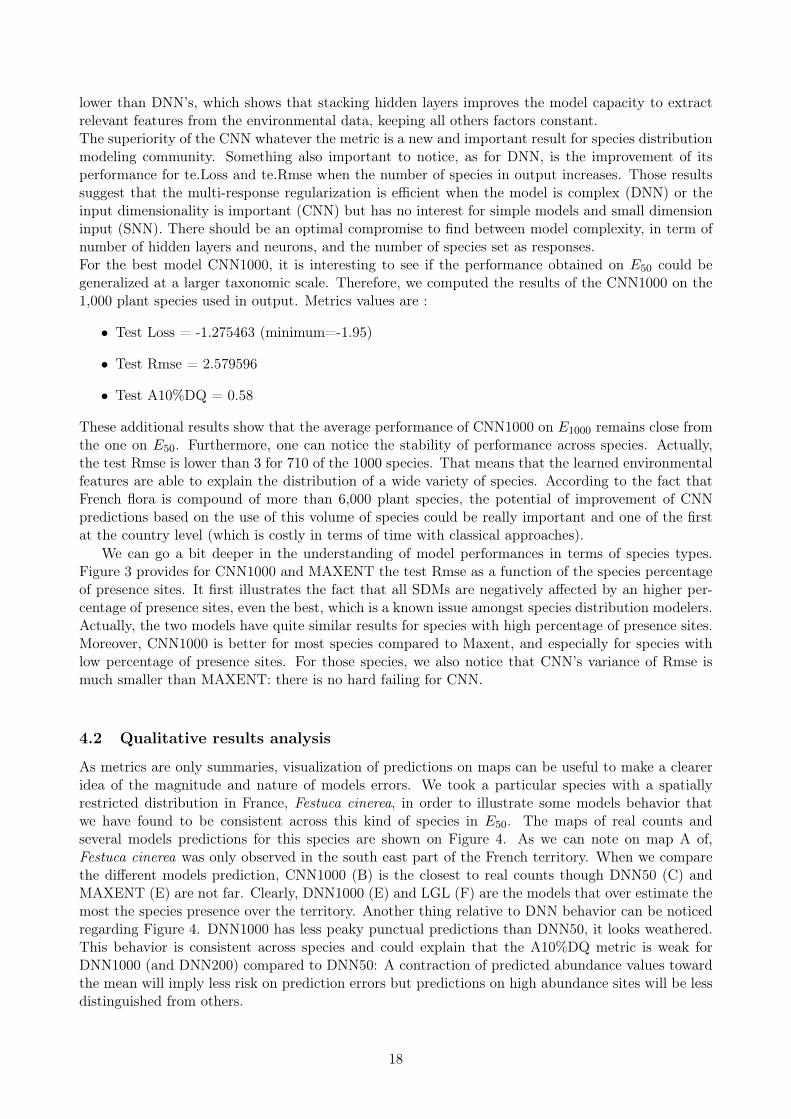

42
44
46
48
50
minus5 0 5Longitude
Latit
ude
vale
(minus2minus01]
(minus0105]
(051]
(12]
(23]
(34]
(46]
(610]
(1016]
(1625]
(2540]
(4063]
(63100]
(100158]
Counts of Festuca cinerea Vill in INPN
Values
42
44
46
48
50
minus5 0 5Longitude
Latit
ude
vale
(minus2minus01]
(minus0105]
(051]
(12]
(23]
(34]
(46]
(610]
(1016]
(1625]
(2540]
(4063]
(63100]
(100158]
Counts of Anthriscus sylvestris (L) Hoffm in INPN
42
44
46
48
50
minus5 0 5Longitude
Latit
ude
vale
(minus2minus01]
(minus0105]
(051]
(12]
(23]
(34]
(46]
(610]
(1016]
(1625]
(2540]
(4063]
(63100]
Predicted counts of Anthriscus sylvestris (L) Hoffm with MAXENT
42
44
46
48
50
minus5 0 5Longitude
Latit
ude
vale
(minus2minus01]
(minus0105]
(051]
(12]
(23]
(34]
(46]
(610]
(1016]
(1625]
(2540]
(4063]
(63100]
Counts of Anthriscus sylvestris (L) Hoffm in patch_CNN1000
42
44
46
48
50
minus5 0 5Longitude
Latit
ude
vale
(minus2minus01]
(minus0105]
(051]
(12]
(23]
(34]
(46]
(610]
(1016]
(1625]
(2540]
(4063]
(63100]
(100158]
(158251]
(251398]
Counts of Ranunculus repens L in INPN
42
44
46
48
50
minus5 0 5Longitude
Latit
ude
vale
(minus2minus01]
(minus0105]
(051]
(12]
(23]
(34]
(46]
(610]
(1016]
(1625]
(2540]
(4063]
(63100]
(100158]
(158251]
Predicted counts of Ranunculus repens L with MAXENT
42
44
46
48
50
minus5 0 5Longitude
Latit
ude
vale
(minus2minus01]
(minus0105]
(051]
(12]
(23]
(34]
(46]
(610]
(1016]
(1625]
(2540]
(4063]
(63100]
(100158]
(158251]
Counts of Ranunculus repens L in patch_CNN1000
Predicted counts ofAnthriscussylvestris with CNN1000
Predicted counts ofAnthriscussylvestris with MAXENT
Counts ofAnthriscus sylvestrisinINPN
Predicted counts ofRanunculusrepenswith CNN1000
Predicted counts ofRanunculusrepenswith MAXENT
Counts ofRanunculus repensinINPN
A)
B)
Figure 5 A) Species occurrences in INPN dataset and geographic distribution predicted with Maxentand CNN1000 for Anthriscus sylvestris (L) Hoffm B) Species occurrences in INPN dataset andgeographic distribution predicted with Maxent and CNN1000 for Ranunculus repens L
5 Discussion
The performance increase with multi-responses models shows that multi-responses architecture arean efficient regularization scheme for NNs in SDM It could be interesting to evaluate the perfor-mance impact of going multi-response on rare species where data are limited We have systematicallynoticed false predicted presence for species that are not in the Mediterranean region It could bedue to a high representativity of species from this region in France In the multi-response modelingthe Mediterranean species could favor prediction in this area through neurons activations rather thanother areas where few species are present inducing bias Thus the distributions complementaritybetween selected species could be an interesting subject for further research
Even if our study presents promising results there are still some open problems A first one isrelated to the bias in the sampling process that is not taken into account in the model Indeed evenif the estimation of bias in the learning process is difficult this could strongly improve our results Biascan be related to the facts that (i) some regions and difficult environments are clearly less inventoriedthan others (this can be seen with empty region in South western part of the country in Figure 4and 5) (ii) some regions are much more inventoried than others according to the human capacitiesof the National botanical conservatories which have very different sizes (iii) some common and lessattractive species for naturalists are not recorded even if they are present in prospected areas whichis a bias due to the use of opportunistic observations rather than exhaustive count data
In the NN models learning there is still work to be done on quick automated procedure for tun-ing optimization hyper-parameters especially the initial learning rate and we are looking for a moresuited stopping rule On the other hand in the case of models of species distributions we can imagineto minimize the number of not null connections in the network to make it more interpretable andintroduce an L1-type penalty on the network parameters This is a potential important perspective
21
of future works
One imperfection in our modeling approach that induces biased distribution estimate is that therepresentation (vector or array of environmental variables) of a site is extracted from its geographiccenter MAXENT SNN and DNN models typically only integrate the central value of the environ-mental variables on each site omitting the variability within the site Instead of that an unbiaseddata generation would sample for each site many representations uniformly in its spatial domain andin number proportional to its area This way it would provide richer information about sites and atthe same time prevent NN model over-fitting by producing more data samples
A deeper analysis of the behavior of the models according to the ecological preferences of the speciescould be of a strong interest for the ecological community This study could allow to see dependencesof the models to particular spatial patterns andor environmental variables Plus it would be inter-esting to check if NN perform better when the species environmental niche is in the intersection ofvariables values that are far from their typical ranges into the study domain which is something thatMAXENT cannot fit
Another interesting perspective for this work is the fact that new detailed fine-scale environmentaldata become freely available with the development of the open data movement in particular thanksto advances in remote sensing methods Nevertheless as long as we only have access to spatiallydegraded observations data at kilometer scales like here it is difficult to consistently estimate theeffect of variables that vary at high frequency in space For example the informative link betweenspecies abundance and land cover proximity to fresh water or proximity to roads is very blurredand almost lost To overcome this difficulty there is much hope in the high flow of finely geolocatedspecies observations produced by citizen sciences programs for plant biodiversity monitoring like TelaBotanica 6 iNaturalist 7 Naturgucker 8 or PlntNet 9 From what we can see on the GBIF10 the first three already have high resolution and large cover observation capacity they have accu-mulated around three hundred thousand finely geolocated plant species observations just in Franceduring last decade Citizen programs in biodiversity sciences are currently developing worldwide Weexpect them to reach similar volumes of observations to the sum of national museums herbaria andconservatories in the next few years while still maintaining a large flow of observations for the futureWith good methods for dealing with sampling bias those fine precision and large spatial scale datawill make a perfect context for reaching the full potential of deep learning SDM methods Thus NNmethods could be a significant tool to explore biodiversity data and extract new ecological knowledgein the future
6 Conclusion
This study is the first one evaluating the potential of the deep learning approach for species distribu-tions modeling It shows that DNN and CNN models trained on 50 plant species of French flora clearlyovercomes classical approaches such as Maxent and LGL used in ecological studies This result ispromising for future ecological studies developed in collaboration with naturalists expert Actuallymany ecological studies are based on models that do not take into account spatial patterns in envi-ronmental variables In this paper we show for a random set of 50 plant species of the French florathat CNN and DNN when learned as multi-species output models are able to automatically learn
6httpwwwtela-botanicaorgsiteaccueil7httpswwwinaturalistorg8httpnaturguckerdeenjoynaturenet9httpsplantnetorgen
10httpswwwgbiforg
22
non-linear transformations of input environmental features that are very relevant for every specieswithout having to think a priori about variables correlation or selection Plus CNN can capture extrainformation contained in spatial patterns of environmental variables in order to surpass other classicalapproaches and even DNN We also did show that the models trained on higher number of species inoutput (from 50 to 1000) stabilize predictions across species or even improve them globally accordingto the results that we got for several metrics used to evaluate them This is probably one the mostimportant outcome of our study It opens new opportunities for the development of ecological studiesbased on the use of CNN and DNN (eg the study of communities) However deeper investigationsregarding specific conditions for models efficiency or the limits of interpretability NN predictionsshould be conducted to build richer ecological models
23
References
Berman Mark amp Turner T Rolf 1992 Approximating point process likelihoods with GLIM AppliedStatistics 31ndash38
Chen Tianqi Li Mu Li Yutian Lin Min Wang Naiyan Wang Minjie Xiao Tianjun Xu BingZhang Chiyuan amp Zhang Zheng 2015 Mxnet A flexible and efficient machine learning libraryfor heterogeneous distributed systems arXiv preprint arXiv151201274
Dutregraveve B Robert S 2016 INPN - Donneacutees flore des CBN agreacutegeacutees par la FCBN Version 11 SPN- Service du Patrimoine naturel Museacuteum national drsquoHistoire naturelle Paris
Fithian William amp Hastie Trevor 2013 Finite-sample equivalence in statistical models for presence-only data The annals of applied statistics 7(4) 1917
Friedman Jerome H 1991 Multivariate adaptive regression splines The annals of statistics 1ndash67
Goodfellow Ian Bengio Yoshua amp Courville Aaron 2016 Deep Learning MIT Press httpwwwdeeplearningbookorg
Hastie Trevor amp Tibshirani Robert 1986 Generalized Additive Models Statistical Science 1(3)297ndash318
Hutchinson G Evelyn 1957 Cold spring harbor symposium on quantitative biology Concludingremarks 22 415ndash427
Ioffe Sergey amp Szegedy Christian 2015 Batch normalization Accelerating deep network training byreducing internal covariate shift Pages 448ndash456 of International Conference on Machine Learning
Karger Dirk N Conrad Olaf Boumlhner Juumlrgen Kawohl Tobias Kreft Holger Soria-Auza Ro-drigo W Zimmermann Niklaus E Linder H Peter amp Kessler Michael 2016a CHELSA clima-tologies at high resolution for the earthrsquos land surface areas (Version 11)
Karger Dirk Nikolaus Conrad Olaf Boumlhner Juumlrgen Kawohl Tobias Kreft Holger Soria-AuzaRodrigo Wilber Zimmermann Niklaus Linder H Peter amp Kessler Michael 2016b Climatologiesat high resolution for the earthrsquos land surface areas arXiv preprint arXiv160700217
Krizhevsky Alex Sutskever Ilya amp Hinton Geoffrey E 2012 Imagenet classification with deepconvolutional neural networks Pages 1097ndash1105 of Advances in neural information processingsystems
Leathwick JR Elith J amp Hastie T 2006 Comparative performance of generalized additive mod-els and multivariate adaptive regression splines for statistical modelling of species distributionsEcological modelling 199(2) 188ndash196
LeCun Yann et al 1989 Generalization and network design strategies Connectionism in perspec-tive 143ndash155
Lek Sovan Delacoste Marc Baran Philippe Dimopoulos Ioannis Lauga Jacques amp AulagnierSteacutephane 1996 Application of neural networks to modelling nonlinear relationships in ecologyEcological modelling 90(1) 39ndash52
Nair Vinod amp Hinton Geoffrey E 2010 Rectified linear units improve restricted boltzmann ma-chines Pages 807ndash814 of Proceedings of the 27th international conference on machine learning(ICML-10)
24
P Anderson Robert Dudiacutek Miroslav Ferrier Simon Guisan Antoine J Hijmans RobertHuettmann Falk R Leathwick John Lehmann Anthony Li Jin G Lohmann Lucia et al 2006 Novel methods improve prediction of speciesrsquo distributions from occurrence data Ecography29(2) 129ndash151
Panagos Panos 2006 The European soil database GEO connexion 5(7) 32ndash33
Panagos Panos Van Liedekerke Marc Jones Arwyn amp Montanarella Luca 2012 European SoilData Centre Response to European policy support and public data requirements Land Use Policy29(2) 329ndash338
Phillips Steven J amp Dudiacutek Miroslav 2008 Modeling of species distributions with Maxent newextensions and a comprehensive evaluation Ecography 31(2) 161ndash175
Phillips Steven J Dudiacutek Miroslav amp Schapire Robert E 2004 A maximum entropy approach tospecies distribution modeling Page 83 of Proceedings of the twenty-first international conferenceon Machine learning ACM
Phillips Steven J Anderson Robert P amp Schapire Robert E 2006 Maximum entropy modeling ofspecies geographic distributions Ecological modelling 190(3) 231ndash259
Phillips Steven J Anderson Robert P Dudiacutek Miroslav Schapire Robert E amp Blair Mary E 2017Opening the black box an open-source release of Maxent Ecography
Rumelhart David E Hinton Geoffrey E Williams Ronald J et al 1988 Learning representationsby back-propagating errors Cognitive modeling 5(3) 1
Thuiller Wilfried 2003 BIOMODndashoptimizing predictions of species distributions and projectingpotential future shifts under global change Global change biology 9(10) 1353ndash1362
Van Liedekerke M Jones A amp Panagos P 2006 ESDBv2 Raster Library-a set of rasters derivedfrom the European Soil Database distribution v2 0 European Commission and the European SoilBureau Network CDROM EUR 19945
Ward Gill Hastie Trevor Barry Simon Elith Jane amp Leathwick John R 2009 Presence-onlydata and the EM algorithm Biometrics 65(2) 554ndash563
Zomer Robert J Bossio Deborah A Trabucco Antonio Yuanjie Li Gupta Diwan C amp SinghVirendra P 2007 Trees and water smallholder agroforestry on irrigated lands in Northern IndiaVol 122 IWMI
Zomer Robert J Trabucco Antonio Bossio Deborah A amp Verchot Louis V 2008 Climate changemitigation A spatial analysis of global land suitability for clean development mechanism afforesta-tion and reforestation Agriculture ecosystems amp environment 126(1) 67ndash80
25
- Introduction
-
- Context on species distribution models
- Interest of deep and convolutional neural networks for SDM
- Contribution
-
- A Deep learning model for SDM
-
- A large-scale Poisson count model
- Links with MAXENT
- SDM based on a fully-connected NN model
- SDM based on a convolutional NN model
-
- Data and methods
-
- Observations data of INPN
- Species selection
- Environnemental data
-
- Climatic descriptors Chelsea Climate data 11
- Potential Evapotranspiration CGIAR-CSI ETP data
- Pedologic descriptors The ESDB v2 - 1kmx1km Raster Library
- Altitude USGS Digital Elevation data
- Hydrographic descriptor BD Carthage v3
- Land cover Corine Land Cover 2012 version 1851 122016
- Environmental variables extraction and format
-
- Detailed models architectures and learning protocol
-
- Baseline models
- Proposed models based on NN
- Models optimization
-
- Evaluation metrics
-
- Results
-
- Quantitative results analysis
- Qualitative results analysis
-
- Discussion
- Conclusion
-