a decision support system for selecting it audit areas

A decision support system for selecting IT audit areas using a capital budgeting

approach

DP Pieters

20795017

Dissertation submitted in partial fulfilment of the requirements for the degree Magister Scientiae in Computer Science at the

Potchefstroom Campus of the North-West University

Supervisor: Prof HA Kruger

Co-supervisor: Mr WD Kearney

May 2015

i

ABSTRACT

Internal audit departments strive to control risk within an organization. To do this they

choose specific audit areas to include in an audit plan. In order to select areas, they usually

focus on those areas with the highest risk. Even though high risk areas are considered, there

are various other restrictions such as resource constraints (in terms of funds, manpower and

hours) that must also be considered. In some cases, management might also have special

requirements. Traditionally this area selection process is conducted using manual processes

and requires significant decision maker experience. This makes it difficult to take all

possibilities into consideration while also catering for all resource constraints and special

management requirements. In this study, mathematical techniques used in capital

budgeting problems are explored to solve the IT audit area selection problem. A DSS is

developed which implements some of these mathematical techniques such as a linear

programming model, greedy heuristic, improved greedy heuristic and evolutionary heuristic.

The DSS also implements extensions to the standard capital budgeting model to make

provision for special management requirements. The performance of the mathematical

techniques in the DSS is tested by applying different decision rules to each of the techniques

and comparing those results. The DSS, empirical experiments and results are also presented

in this research study. Results have shown that in most cases a binary 0-1 model

outperformed the other techniques. Internal audit management should therefore consider

this model to assist with the construction of an IT internal audit plan.

Keywords: IT audit plan, capital budgeting, linear programming, integer programming,

heuristics, decision support system (DSS).

ii

OPSOMMING

Interne oudit departemente streef daarna om risiko binne 'n organisasie te beheer. Om dit te

doen kies hulle spesifieke oudit areas om in te sluit in 'n oudit plan. Die keuse van areas is

gewoonlik gefokus op die areas met die hoogste risiko. Selfs al word hoë risiko areas

oorweeg, is daar verskeie ander beperkinge soos beperkte hulpbronne (in terme van fondse,

mannekrag en ure) wat ook in ag geneem moet word. In sommige gevalle kan bestuur ook

spesiale vereistes hê. Tradisioneel word die kies van areas uitgevoer met behulp van hand

seleksie prosesse en vereis betekenisvolle besluitnemerservaring. Hierdie manier van

seleksie maak dit moeilik om alle moontlikhede in ag te neem, aangesien daar ook

voorsiening gemaak moet word vir beperkte hulpbronne en spesiale bestuursvereistes. In

hierdie studie word wiskundige tegnieke verken wat in kapitaalbegroting probleme gebruik

word, om die IT-oudit areaseleksie probleem op te los. 'n Besluitnemingsondersteuning-

stelsel is ontwikkel wat sommige van hierdie wiskundige tegnieke, soos 'n lineêre

programmeringsmodel, gulsig heuristiek, verbeterde gulsig heuristiek en evolusionêre

heuristiek te implementeer. Die besluitnemingsondersteuningstelsel implementeer ook

uitbreidings van die standaard kapitaalbegrotingsmodel om voorsiening te maak vir spesiale

bestuursvereistes. Die wiskundige tegnieke in die besluitnemingsondersteuningstelsel word

getoets deur verskillende besluitnemingsreëls toe te pas op elke tegniek en die resultate te

vergelyk en te evalueer. Die besluitnemingsondersteuningstelsel, empiriese eksperimente en

resultate word ook in hierdie navorsingstudie voorgehou. Resultate het aangetoon dat „n

binêre 0-1 model in meeste gevalle beter vaar as die ander tegnieke. Die bestuur van „n

interne oudit departement behoort dus hierdie tipe model te oorweeg as hulpmiddel vir die

opstelling van „n IT interne oudit plan.

Sleutelwoorde: IT-oudit plan, kapitaalbegroting, lineêre programmering, heeltallige

programmering, heuristieke, besluitnemingsondersteuningstelsel.

iii

ACKNOWLEDGEMENTS

I would like to thank my supervisor, Prof. H.A. Kruger for all his input, advice, expertise and

guidance throughout this study. I would also like to acknowledge my co-supervisor, Mr W.D.

Kearney for his input, as well as thank the Australian company that provided me with the

dataset without which this study would not have been possible.

Furthermore, I would like to thank my family and friends who supported and inspired me

during this study.

Above all, I give praise to my Lord and Saviour for giving me the capability and endurance to

complete this research project.

iv

Table of Contents

1. Introduction and problem statement ........................................................... 1

1.1 Introduction ................................................................................................................ 1

1.2 Problem statement ...................................................................................................... 1

1.3 Study objectives ........................................................................................................... 2

1.4 Research methodology ................................................................................................ 3

1.5 Chapter overview......................................................................................................... 3

1.6 Chapter summary ........................................................................................................ 4

2. Literature review and background ............................................................... 5

2.1 Introduction ................................................................................................................ 5

2.2 Definition of internal auditing .................................................................................... 5

2.3 Information technology auditing ................................................................................ 6

2.3.1 Introduction and definition ................................................................................. 6

2.3.2 Information technology audit planning............................................................... 6

2.3.2.1 Understand the business .................................................................................. 8

2.3.2.2 Defining the IT universe ................................................................................... 9

2.3.2.3 Risk assessment................................................................................................ 9

2.3.2.4 Formalize audit plan ........................................................................................ 9

2.4 Risk assessment ........................................................................................................ 10

2.4.1 Introduction and definition ............................................................................... 10

2.4.2 Quantitative and qualitative methods to determine risk .................................... 11

2.5 Capital budgeting ...................................................................................................... 14

2.5.1 Introduction and definition ............................................................................... 14

2.5.2 Capital budgeting evaluation techniques........................................................... 15

2.5.2.1 Net present value ............................................................................................ 16

2.5.2.2 Internal rate of return .................................................................................... 17

2.5.2.3 Discounted payback ....................................................................................... 18

2.5.2.4 Payback period ............................................................................................... 18

2.5.2.5 Profitability index ........................................................................................... 19

2.5.2.6 Accounting rate of return ...............................................................................20

2.5.3 Related work using capital budgeting techniques ............................................. 21

2.6 Chapter summary ...................................................................................................... 22

3. Mathematical programming techniques .................................................... 24

3.1 Introduction .............................................................................................................. 24

3.2 Linear programming ................................................................................................. 24

3.2.1 Introduction ....................................................................................................... 24

v

3.2.2 Linear program model formulation ................................................................... 25

3.2.3 Basic assumptions of a linear programming model .......................................... 26

3.2.4 Methods to solve ................................................................................................ 27

3.2.4.1 Graphical methods ......................................................................................... 27

3.2.4.1.1 Iso-profit line method ............................................................................ 27

3.2.4.1.2 Corner point method ............................................................................. 28

3.2.4.1.3 Special cases .......................................................................................... 29

3.2.4.2 Simplex Method ............................................................................................. 33

3.2.5 Sensitivity analysis ............................................................................................. 35

3.3 Integer programming ................................................................................................ 36

3.3.1 Introduction ....................................................................................................... 36

3.3.2 Integer programming model formulation ......................................................... 36

3.3.3 Methods to solve ................................................................................................ 37

3.3.3.1 Cutting plane technique ................................................................................. 37

3.3.3.2 Enumerative methods .................................................................................... 38

3.3.4 Logical conditions .............................................................................................. 39

3.3.4.1 Limit the number of alternatives ................................................................... 39

3.3.4.2 Dependent selections .................................................................................... 40

3.3.4.3 Lot size constraints ........................................................................................ 40

3.3.4.4 K of m constraints .......................................................................................... 41

3.4 Capital budgeting ...................................................................................................... 41

3.4.1 Capital budgeting extensions ............................................................................. 42

3.4.1.1 Projects of different lengths ........................................................................... 43

3.4.1.2 Adding capital inflows from completed projects ........................................... 43

3.4.1.3 Projects with staged returns ........................................................................... 44

3.4.1.4 Carrying unused capital forward from year to year ....................................... 44

3.4.1.5 Mutually exclusive and sequential projects ................................................... 44

3.4.1.6 Projects with different start/end dates .......................................................... 45

3.4.1.7 Projects with a time window for the start time .............................................. 45

3.5 The capital budgeting problem applied to the selection of IT audit areas................ 45

3.6 Chapter summary ...................................................................................................... 46

4. Heuristic programming techniques ........................................................... 47

4.1 Introduction .............................................................................................................. 47

4.2 Heuristic methods ..................................................................................................... 47

4.2.1 Greedy heuristic methods .................................................................................. 47

4.2.1.1 Greedy heuristic ............................................................................................. 48

4.2.1.2 Improved greedy heuristic ............................................................................. 49

vi

4.2.1.3 „Greedy and swap‟ heuristic to solve integer programming problems ........... 50

4.2.2 Evolutionary heuristic method .......................................................................... 51

4.2.3 Motivation for selecting heuristics to be included in DSS ................................. 55

4.3 Chapter summary ...................................................................................................... 57

5. DSS for selecting IT audit areas ................................................................. 58

5.1 Introduction .............................................................................................................. 58

5.2 Decision support systems.......................................................................................... 58

5.3 DSS development ...................................................................................................... 67

5.3.1 Normal analysis .................................................................................................68

5.3.1.1 Include areas .................................................................................................. 69

5.3.1.2 Exclude areas .................................................................................................. 71

5.3.1.3 Include/exclude multiple IT audit areas from sub lists ................................. 71

5.3.1.4 Dependencies ................................................................................................. 72

5.3.1.4.1 Normal dependencies ............................................................................ 72

5.3.1.4.2 Risk dependencies ................................................................................. 73

5.3.2 Grouped analysis ............................................................................................... 75

5.3.2.1 Include groups of areas .................................................................................. 75

5.3.2.2 Exclude groups of areas.................................................................................. 78

5.4 Chapter summary ...................................................................................................... 79

6. Empirical experiments and results ............................................................ 80

6.1 Introduction ............................................................................................................. 80

6.2 Data collection and processing ................................................................................ 80

6.3 Comparative criteria ................................................................................................. 83

6.3.1 Risk coverage ..................................................................................................... 83

6.3.2 Resource utilization ........................................................................................... 84

6.3.3 Model formulation complexity .......................................................................... 84

6.3.4 Baseline computation time deviation ................................................................ 85

6.4 The experiments ........................................................................................................86

6.4.1 Experiment 1 (Normal analysis) – No decision rules ........................................ 87

6.4.2 Experiment 2 (Normal analysis) – Exclude specific IT audit areas ................. 90

6.4.3 Experiment 3 (Normal analysis) – Include specific IT audit areas ................... 94

6.4.4 Experiment 4 (Normal analysis) – Include/Exclude a number of ........................

IT audit areas .....................................................................................................98

6.4.5 Experiment 5 (Normal analysis) – Add normal dependencies among .................

specific IT audit areas ...................................................................................... 101

6.4.6 Experiment 6 (Normal analysis) – Add risk dependencies among .......................

specific IT audit areas ...................................................................................... 104

vii

6.4.7 Experiment 7 (Grouped analysis) .................................................................... 109

6.5 General discussion, recommendations and contribution ....................................... 109

6.5.1 The use of a mathematical technique to construct an IT audit plan ............... 109

6.5.2 The decision support system (DSS) .................................................................. 111

6.6 Chapter summary ..................................................................................................... 113

7. Summary and conclusions ........................................................................ 114

7.1 Introduction ............................................................................................................. 114

7.2 Objectives of the research study............................................................................... 114

7.3 Problems experienced .............................................................................................. 117

7.4 Possible further research ......................................................................................... 117

7.5 Chapter summary .................................................................................................... 118

Appendix A ..................................................................................................... 119

A.1 DSS system requirements ........................................................................................ 119

Bibliography .................................................................................................. 120

viii

List of Figures

Chapter 2: Literature review and background

Figure 2.1: Logical work-flow progression for an IT audit plan process .................................. 7

Chapter 3: Mathematical programming techniques

Figure 3.1: Graphical solution to example 1 ............................................................................ 29

Figure 3.2: Infeasible solution ................................................................................................30

Figure 3.3: Unboundedness .................................................................................................... 31

Figure 3.4: Redundancy .......................................................................................................... 32

Figure 3.5: Alternate optimal solutions .................................................................................. 33

Chapter 5: DSS for selecting IT audit areas

Figure 5.1: Business Pressures-Responses-Support Model .................................................... 59

Figure 5.2: Decision making process ...................................................................................... 62

Figure 5.3: Ideal characteristics and capabilities of a DSS ..................................................... 63

Figure 5.4: DSS - schematic view. ........................................................................................... 66

Figure 5.5: High level structure of the DSS ............................................................................68

Chapter 6: Empirical experiments and results

Figure 6.1: Experiment 1 - Model formulation complexity .....................................................89

Figure 6.2: Experiment 1 – DSS results ..................................................................................89

Figure 6.3: Experiment 2 - Model formulation complexity .................................................... 92

Figure 6.4: Experiment 2 - DSS results .................................................................................. 93

Figure 6.5: Experiment 3 - Model formulation complexity .................................................... 96

Figure 6.6: Experiment 3 – DSS results ................................................................................. 97

Figure 6.7: Experiment 4 - Model formulation complexity .................................................. 100

Figure 6.8: Experiment 4 – DSS results ............................................................................... 100

Figure 6.9: Experiment 5 - Model formulation complexity .................................................. 103

Figure 6.10: Experiment 5 – DSS results .............................................................................. 104

Figure 6.11: Experiment 6 - Model formulation complexity ................................................ 107

Figure 6.12: Experiment 6 – DSS results .............................................................................. 108

ix

List of Tables

Chapter 2: Literature review and background

Table 2.1: Advantages and disadvantages of quantitative and qualitative methods .............. 13

Table 2.2: Comparison of capital budgeting process stages ................................................... 15

Table 2.3: Classification of capital budgeting evaluation techniques ..................................... 16

Table 2.4: Advantages and disadvantages of payback evaluation technique ......................... 19

Table 2.5: Advantages and disadvantages of the accounting rate of return evaluation

technique................................................................................................................20

Chapter 3: Mathematical programming techniques

Table 3.1: Initial simplex tableau ............................................................................................ 34

Table 3.2: Projects‟ characteristics ......................................................................................... 42

Chapter 4: Heuristic programming techniques

Table 4.1: Initial population .................................................................................................... 52

Table 4.2: Crossover and Mutation ......................................................................................... 53

Table 4.3: New Population ...................................................................................................... 53

Table 4.4: Differences between classical and genetic algorithms ........................................... 54

Table 4.5: List of IT audit areas .............................................................................................. 54

Chapter 5: DSS for selecting IT audit areas

Table 5.1: Reasons for using computerized DSS‟s ................................................................. 60

Table 5.2: IT audit areas to include ........................................................................................ 69

Table 5.3: List of IT audit areas available for selection .......................................................... 70

Table 5.4: List of IT audit areas after adding risk dependency .............................................. 74

Table 5.5: IT audit areas to include ........................................................................................ 76



Chapter 6: Empirical experiments and results

Table 6.1: IT audit area dataset ............................................................................................... 83

Table 6.2: Experiments conducted .........................................................................................86

Table 6.3: Experiment 1 – Comparative criteria results ........................................................ 88




Table 6.7: Experiment 5 – Comparative criteria results ....................................................... 103

Table 6.8: Experiment 6 – Comparative criteria .................................................................. 107

1

Chapter 1

1. Introduction and problem statement

1.1 Introduction

All modern organizations have internal audit departments, and some of the goals of an

internal audit department is to monitor and control risks (Sobel, 2011). This is usually done

by choosing specific audit areas, including IT audit areas, with high risks. These selected

audit areas will then be presented in an audit plan, after which the audit will be focused on

the areas with the highest risk. The choice of areas to be included in the IT audit plan relies

heavily on discussions between the stakeholders as well as the experience of the decision

makers. The quality of the decisions has a great impact on the outcome of the audit. To

make quality decisions require assessment and analysis of data which will either lead to a

good or a bad decision. A good decision is mostly obtained through following a sequence of

analytical steps by using quantitative approaches. A decision support system (DSS) provides

an efficient, effective and user friendly way to implement mathematical techniques that

apply a quantitative approach to decision making, which can optimize stakeholder decision

making. Currently, mathematical techniques to assist with the construction of audit plans,

i.e. the selection of suitable audit areas, are not utilized widely in internal audit

environments. They are, however, utilized in capital budgeting problems where a selection

of projects from a proposed list of projects has to be made. This implies the maximization of

the value of the projects selected subject to certain limitations such as a budget and

manpower. This approach relates closely to the selection of IT audit areas for inclusion in an

IT audit plan. It therefore makes sense to adapt the mathematical models used in capital

budgeting and implement these adapted models in a DSS to assist with the process of

selecting IT audit areas.

The purpose of this chapter is to present an introduction to the research project by

explaining the problem statement, objectives of the study and the methodology that will be

followed. A layout of the study, explaining the purpose of each chapter, is also presented.

1.2 Problem statement

When an audit plan is constructed, audit resources are usually constrained. This means that

not all audit areas can be audited every year and therefore only those with a high risk should

be selected (Roslewicz, 1994). Even if there is a risk factor available for each of the audit

2

areas, it is still difficult to choose the right areas. The reason for this is twofold. Firstly, the

costs to audit different areas, the amount of resources (number of workers) needed to

conduct the audits and the time (number of hours) required to audit different areas, may

differ. Regardless of these differences, management also has specific requirements (e.g.

some of the audit areas are related to each other so that when one area is audited, it may lead

to a lowering of another audit area‟s risk factor). These requirements (decision rules) are

very difficult to implement using the traditional manual processes followed. Secondly, audit

plans are customarily created through discussions and agreement between the organization‟s

stakeholders. Although this decision is normally based on a risk rating process, it only

distinguishes between high, medium and low risk and relies heavily on the experience of the

decision makers. Therefore, the selection of areas to include in the IT audit plan is not

necessarily the optimal or best combination of areas (taking into account all resource

constraints and unique requirements) and might be improved using mathematical

techniques.

To address these problems, the research study will adapt and evaluate different

mathematical and heuristic programming techniques usually used for capital budgeting

problems, and apply them in internal auditing to select appropriate IT areas for audit. This

will be implemented in a DSS. To cater for special management requirements, the DSS

allows the decision maker to add unique requirements such as to include or exclude specific

IT audit areas, or to add relationships (dependencies) among areas. These unique

requirements will be implemented by taking possible extensions of a capital budgeting

approach and adapting them to fit the IT audit area selection problem.

1.3 Study objectives

The primary objective of the study is to develop a DSS that employs different mathematical

techniques, based on a capital budgeting approach, to solve the IT audit area selection

problem. In order to achieve this, the following five secondary research objectives will be

addressed:

gain a good understanding of the audit area selection problem;

gain a good understanding of capital budgeting problems and existing evaluation

techniques;

investigate possible mathematical techniques in order to identify feasible

techniques for implementation in the DSS;

gain a clear understanding of DSS‟s and develop a DSS to construct an IT audit

plan using mathematical techniques; and

3

evaluate how the mathematical techniques perform using real world data and

scenarios.

1.4 Research methodology

The research study consists of four parts namely a literature study, mathematical technique

investigation, a DSS development phase and an empirical study. The literature review

provides an overview of auditing, capital budgeting and DSS‟s. The mathematical technique

study investigates the mathematical programming techniques, heuristic programming

techniques and extensions based on the capital budgeting approach in order to select

mathematical techniques for implementation in the DSS. It also includes the modification of

the general capital budgeting approach to fit the IT audit area selection problem. This will be

followed by the DSS development and implementation of the mathematical techniques and

extensions in the DSS. Lastly, empirical experiments will be conducted to evaluate the

performance of the mathematical techniques implemented in the DSS when specific

requirements (extensions) exist, using real world data and requirements.

1.5 Chapter overview

This section outlines the purpose and structure of each chapter.

Chapter 2 presents a literature overview of auditing and capital budgeting. IT audits and the

construction of an IT audit plan will be briefly looked at, followed by an overview of risk-

based auditing and some of the existing methods to compute an audit area‟s risk. The

chapter will also discuss capital budgeting and techniques to evaluate capital budgeting

problems.

Chapter 3 investigates linear programming models. The basic assumptions of linear

programming models and different existing mathematical methods to solve linear

programming models will be discussed. Different types of integer models will also be

presented. Logical conditions which form an important part of the study will be explained.

The standard linear programming model and different extensions to solve a capital

budgeting problem will be discussed using examples. The chapter will also discuss how the

capital budgeting approach will be applied to the selection of IT audit areas.

Chapter 4 introduces and investigates several heuristic programming techniques used in

capital budgeting. The implementation of these heuristic techniques will be discussed, after

which a motivation will be provided to clarify which of these heuristic techniques were

implemented in the DSS with appropriate reasons.

4

Chapter 5 applies the adapted capital budgeting model to the IT audit area selection problem

by developing a DSS. A brief overview of DSS‟s provides background information. The

implementation of the chosen mathematical techniques will be described as well as how

these techniques handle each of the different decision rules in the DSS. Appropriate

examples and mathematical formulations will also be presented where necessary.

Chapter 6 presents the real world data and explains the experiments and their results. The

results of the empirical study will be evaluated, after which a general discussion and

recommendations are provided.

Finally, Chapter 7 summarizes all objectives set out for the study and how these were

addressed and achieved. The chapter will also present the problems experienced during the

study and point out opportunities for further studies.

1.6 Chapter summary

Chapter 1 provided an introduction to the research study by explaining the problem

statement, objectives and research methodology that will be followed. A layout of the study,

explaining the purpose of each chapter, was also presented. The next chapter will present a

literature overview of auditing and capital budgeting.

5

Chapter 2

2. Literature review and background

2.1 Introduction

The primary objective of this study is to investigate the use of capital budgeting techniques to

select IT audit areas from an internal IT audit plan. To gain a good understanding of the

concepts and techniques that will be used in the subsequent chapters, this chapter will act as

an introductory overview to internal auditing, risk assessment and capital budgeting.

The chapter starts with a definition of internal auditing and will describe and define IT

auditing, which is a newer arrival to the auditing world. A description of an audit plan will

be given, including the steps that should be followed to create an IT audit plan. Next, a

definition of risk and risk-based auditing will be discussed, followed by an introduction to

some of the existing methods used to compute the risk of an audit area. An explanation of

the risk assessment process for auditing will also be given. Lastly, capital budgeting will be

discussed, including the techniques used to evaluate capital budgeting problems.

2.2 Definition of internal auditing

Internal audit is a control function that can be found in all major organizations. The main

purpose of internal auditing is to help organizations achieve their objectives by evaluating

and improving certain processes such as risk management, governance and more.

Furthermore, different types of audits exist namely financial, operational and IT audits.

Each type of audit may be defined differently.

Chou et al. (2007) defines auditing as “a process that estimates the degree to which the

assertions of a corporation correspond with certain established criteria, such as specific

corporate rules, policies and constraints, or generally accepted accounting principles

(GAAP) that are established by the Financial Accounting Standards Board (FASB) and

other authoritative bodies.” To organize and execute this auditing process, constraints such

as labour and cost are required. Auditors will not monitor every single business transaction,

but instead they rely on supporting evidence known as audit evidence in order to test and

assure the trustworthiness and relevance of information. A similar definition for auditing

can be found in the ISO 19011 (2011) standard which describes an audit to be a “systematic,

independent and documented process for obtaining audit evidence and evaluating it

objectively to determine the extent to which the audit criteria are fulfilled”.

6

Stated earlier, there are different types of audits. One important type that stands out is IT

auditing. IT auditing is important for this study. As mentioned in Chapter 1, this research

study is focused on the selection of IT audit areas by making use of certain mathematical

models. IT audit areas are at the heart of this study and will therefore be discussed in more

detail in the following section.

2.3 Information technology auditing

2.3.1 Introduction and definition

Information technology auditing has become one of the most important control functions

within organizations. The advancements in computer technology lead to organizations

becoming increasingly more dependent on computer information systems to perform

business operations. This increase in the use of information technology also increased the

vulnerabilities and threats organizations have to manage effectively. Each of these

vulnerabilities pose a risk to the organization and thus, choosing which IT audit areas to

audit in an IT audit plan, requires taking these risk factors into account (ASOSAI, 2003). In

this section a short definition of IT auditing will be given, followed by a discussion on IT

audit planning.

IT auditing involves the examination of all the IT business processes and data that integrate

with an organization‟s systems and can be defined as “carefully planned processes that focus

on high-risk areas within the organization” (Carlin & Gallegos, 2007). The ISO 19011

(2002) standard also defines an IT audit as “a systematic, independent and documented

process for obtaining audit evidence and evaluating it objectively to determine the extent to

which the audit criteria are fulfilled”. ISO 19011‟s definition speaks of obtaining audit

evidence which can also be found in the definition given by Weber (1999), who defines an IT

audit as “the process of collecting and evaluating evidence to determine whether a

computer system safeguards assets, maintains data integrity, allows organizational goals

to be achieved effectively and uses resources efficiently”.

To conduct an IT audit effectively and precise, there must be a clear understanding of the

strategy the organization follows. This can be accomplished by preparing an IT audit plan,

which will be described in the next section.

2.3.2 Information technology audit planning

IT audit planning has significant importance in the auditing process. This importance is

comprehensively explained in the ISO 19011 (2011) standard and includes the following

aspects.

7

An audit plan ensures that audit assistants can be properly utilized and that the work to be

done can be coordinated. Using an audit plan enables the auditor to conduct audits

effectively and in a timely and efficient manner, because it ensures that important areas of

the audit receive appropriate attention. It ensures that potential problems can quickly be

identified and that the work to be done is completed on time. Audit planning is also

important because it aids the auditor in acquiring adequate knowledge of the client business

in order to be able to assess both the accounting estimates and management representations‟

reasonableness.

Other researchers and sources also consistently points out the importance of an audit plan,

for example, Rehage et al. (2008) points to the fact that an IT audit plan provides sufficient

coverage on areas of greatest risk as well as those that can add value to an organization.

An audit plan can be defined as a “description of the activities and arrangements for an

audit” (ISO 19011, 2011). According to ISA 300 (2009), an audit plan is a detailed

programme that gives instructions on how to conduct each area of the audit, which means

that it provides details on the specific procedures that need to be carried out.

In order to define an annual IT audit plan, it is important to use a systematic process which

ensures that all necessary business aspects and IT-service support activities are considered

and understood (Rehage et al., 2008). Figure 2.1 depicts an IT audit plan process.

Figure 2.1: Logical work-flow progression for an IT audit plan process (Rehage et al., 2008)

From Figure 2.1 it can be seen that four major steps have to be completed during the

planning process. The following paragraphs will briefly look at each of these four steps.

8

2.3.2.1 Understand the business

Step one in defining the IT audit plan is to understand the business. It is therefore

important to start with the right perspective, which is that technology exists only to support

and further the objectives of the organization and also that technology poses a risk to the

organization as soon as its failure could result in an inability of the business to achieve its

objectives. This means it is important to understand the objectives, business model and

strategies of the organization as well as the role technology plays in supporting the business.

To do this, the risks imposed by the technologies used need to be identified as well as how

each of those risks might prevent the organization‟s achievement of the business objectives.

Every organization differs in terms of business models, IT environments, objectives, delivery

models and organizational structures. Audit plans should therefore be uniquely defined for

each organization. This leads to each organization having a unique set of business risks. It is

also important to understand the structure of the business processes as well as the

organization‟s entity-level strategic objectives, so that auditors can become familiar with the

organization.

Next, the key processes, critical to the success of the objectives, need to be identified.

Processes where failure can prevent an organization from achieving its strategic objectives

are usually considered the key processes. After the key processes have been identified, the

auditors have to outline significant applications and their supporting critical IT

infrastructure. Supporting IT processes such as operations, system development life cycles,

security activities and change management underlie these IT infrastructures and

applications. Therefore, it is critical to examine the operating environment. It will aid the

auditors in understanding and inventorying each of the critical components. An all-inclusive

understanding of technology factors that has an influence on, and helps categorize

organizational risks, is needed to fully comprehend the operating environment and its

associated risks.

There are several different analysis techniques and factors that have to be considered in

order to comprehend the operational environment and its unique risks. The reason for this

is that an organization‟s control environment complexity will have a direct effect on its

overall risk profile and system of internal control. The following eight IT environment

factors have to be taken into consideration:

The degree of system and geographic centralization;

The technologies deployed;

The degree of customization;

9

The degree of formalized company policies and standards;

The degree of regulation and compliance;

The degree and method of outsourcing;

The degree of operational standards; and

The level of reliance on technology.

These factors, in conjunction with the systematic process, can be used to gain a good

understanding of the organization‟s IT infrastructure and operations. Without this

information auditors will not be able to define the IT audit universe and perform the risk

assessment process (Rehage et al., 2008). The next step in constructing an audit plan is to

define the IT universe.

2.3.2.2 Defining the IT universe

According to Rehage et al. (2008), an IT universe is “a finite and all-encompassing

collection of audit areas, organizational entities, and locations identifying business

functions that could be audited to provide adequate assurance on the organization’s risk

management level.” In this phase potential audit areas have to be identified within the IT

universe independently from the risk assessment process. It is important for auditors to be

conscious of what audits can be performed before the process of assessing and ranking risks

can be done. The IT environment has to be divided up into individual audit subjects to

provide audits that are most effective and efficient. Personal preferences could influence

these choices.

2.3.2.3 Risk assessment

After establishing an IT universe inventory, a risk rating needs to be assigned to all sub-

categories which include applications, computer operations and infrastructure. This step is

followed by the ranking of these sub-categories according to the impact they might have on

the organization, as well as the likelihood of the risk occurring. Each of these risks may

differ in terms of their significance or weights across the IT audit universe. Risk assessment

will be discussed in more detail later on in Section 2.4.

2.3.2.4 Formalize audit plan

The final step in defining and creating the audit plan is formalizing the audit plan. This

includes selecting the audit subjects, determining the audit cycle and frequency, adding the

appropriate engagements that are based on the management‟s opportunities and requests,

and validating the plan with the business management. An in depth discussion of this step

can be found in Rehage et al. (2008).

10

To produce an efficient and effective audit plan, all four steps have to be completed

successfully. The third step, risk assessment, appears to be a very significant step in the

process as the selection of audit areas for the final plan relies heavily on a proper risk

assessment. Due to this apparent importance, the next section will elaborate on the risk

assessment stage.

2.4 Risk assessment


To develop an audit plan one has to make use of risks, and in order to be able to use these

risks, one must first understand what risk is. According to Vallabhaneni (1989), risk is “a

potential damaging event that, if it occurs, can produce losses”. Another definition can be

found in the ISO 19011 (2011) standard, which defines risk as an “effect of uncertainty on

objectives”. Ramona (2011) confirms the above mentioned definitions of risk by defining it

as “the potential that a chosen action or activity will lead to a loss”. Combining risks with

auditing has led to a newer arrival to the auditing area namely „risk-based auditing‟ (Lovaas,

2009). According to Ashmore (2011), risk-based auditing is “an approach that focuses on

the response of the organization to the risks it faces in achieving its goals and objectives.

Unlike other forms of audit, risk-based auditing starts with business objectives and their

associated risks rather than the need for controls. It aims to give independent assurance

that risks are being managed to an acceptable level and to facilitate improvements where

necessary”. Other authors, such as Griffiths (2012), describe risk-based auditing as being a

“process, an approach, a methodology and an attitude of mind, rolled into one”. By taking

these definitions into consideration, the concept of risk-based auditing can be understood as

an audit of those things that matter most to an organization which guarantees that a residual

risk falls within the appropriate boundary levels. Except for its role in controlling the

residual risk, risk-based auditing also ensures that an organization conforms to its tolerable

level of risk after the implementation of controls (Griffiths, 2006). The fact that risk-based

auditing focuses on areas in terms of risk instead of concentrating on controls, leads it to

extend and improve the risk assessment process.

For this study the focus does not fall on risk-based auditing but only on risk ratings.

Therefore, only a short definition and description of risk-based auditing was given. An in

depth discussion on risk-based auditing can be found in Griffiths (2006).

Risk ratings that will be used in this study are dependent on the execution of risk

assessments of which a short overview will be given in the following paragraphs.

11

To develop an audit plan includes doing a risk assessment. According to Vallabhaneni

(1989), risk assessment is “an analysis of system assets and vulnerabilities to establish an

expected annual loss or equivalent for certain events based on costs and estimated

probabilities of the occurrence or ranking of the categories of risk of those events”.

Vallabhaneni extends the definition by also describing it as “an analysis of an organization’s

information resources, its existing controls, and its remaining organization and computer

system vulnerabilities. It combines the loss potential for each resource or combination of

resources with an estimated rate of occurrence to establish a potential level of damage to

assets or resources in terms of dollars or other assets”.

To perform the risk assessment process, several steps need to be conducted. According to

Vallabhaneni, the process involves the following steps:

1. Identifying the assets and activities that need protection;

2. Analysing those assets and activities‟ threats and risks;

3. Address these threats and risks by inventorying the controls in place;

4. Match the controls to the risk levels;

5. Perform a cost benefit analysis; and

6. Make recommendations to reduce existing risks and threats.

Step two requires analysis of the possible threats and risks that assets and activities might

impose. This step also involves determining risk ratings by conducting a risk analysis. Two

different approaches, namely a quantitative and qualitative approach, exist to perform this

risk analysis and will be discussed briefly in the next section.

2.4.2 Quantitative and qualitative methods to determine risk

Two different approaches exist to determine risks, namely a qualitative and quantitative

approach. Quantitative approaches use numerical values and assign these values to elements

of the risk assessment. This approach is based on statistical information and is thus

regarded as being more objective than a qualitative approach (PCI SSC, 2012). Using the

quantitative approach, the threats, vulnerabilities and impacts that are associated with an

event, if realized, are presented in the form of an exposure factor. The exposure factor

represents the loss of a resource‟s value in terms of percentage if a threatening event occurs.

Except for the exposure factor, the quantitative approach also takes into account the

probability of an incident occurring. Probability is dependent on the vulnerabilities and

threats with its observation typically taking place within a given time period of valid risk

quantification. The quantitative approach can mathematically be applied to IT risk

assessment as follows (Rot, 2008)

12

(2.1)

(2.2)

where:

– The risk value;

– Probability of an incident occurring and causing loss of assets value within a defined

period of time;

–Predicted loss of an asset‟s value due to a single incident occurrence;

– Threat occurrence frequency; and

– Information system‟s susceptibility on a threat.

Several methods exist to perform risk analysis using a quantitative approach. One of the

most commonly used quantitative methods for risk assessment is the Annual Loss Expected

(ALE) model. As the name states, this model is based on expected loss which is the product

of the probability of occurrence of those events that have a negative impact on IT and values.

This model can mathematically be presented as (Rot, 2008)

∑

(2.3)

where:

– Set that represents the negative effects of events;

– Loss resulting from event , expressed as a value; and

– Frequency of event .

Using this model, an organization‟s annual loss can be determined by the sum of all the

predicted annual losses. Many other models exist to evaluate and assess IT risks which are

based on this ALE method and which are also adapted to fit the specific needs and situations

of organizations. Some of these methods include Courtney‟s model, Information Security

Risk Analysis method and more. A more detailed discussion on these two models can be

found in Rot (2008).

As opposed to the quantitative approach, the qualitative approach uses categorization to

categorize risk parameters according to the impact or intensity level they might have on an

asset. This method does not evaluate the risk in an organization with statistical values, but

instead it uses relative values to act as data entries for the value of possible loss (Ramona,

2011). In short, this means that the qualitative approach does not have numeric values and

13

is an opinion based approach with its results usually summarized using words like „low‟,

„medium‟ or „high‟ (Yazar, 2002).

As with a quantitative approach, the qualitative approach also has several risk assessment

methods available. One such method is called a Risk Classification Matrix (RCM). This

method represents a simple way to rank different potential projects, or in the case of

auditing, audit areas, in terms of their potential benefit and the risks or costs that are likely

to occur when these projects are implemented or audit areas are not audited. Therefore, risk

is not measured, but instead derived from frequency and severity inputs by using the

following formula (Cioacă, 2011)

. (2.4)

In comparing the use of quantitative and qualitative methods, several advantages and

disadvantages come to light. Table 2.1 summarizes some of these advantages and

disadvantages.

Advantages Disadvantages

Quantitative

methods

Allow for definition of consequences

of incident occurrence in a

quantitative way, which facilitates

realization of costs and benefits

analysis during selection of

protections; and

Provides an accurate image of the

risk.

It is dependent on the accuracy and

scope of the defined measurement

scale;

Analysis results may be confusing and

imprecise;

Enrichment of normal methods is

required in qualitative description; and

It is usually more expensive to conduct

such analysis and requires advanced

tools and greater experience.

Qualitative

methods

Risks can be ordered according to

their priority;

Areas that pose a greater risk can be

determined in a short time without

expenditures rising; and

Analysis is cheap and easy to do.

Numerical measures cannot be used to

determine probabilities and results; and

Analysis of costs and benefits is more

difficult during selection of protections.

Table 2.1: Advantages and disadvantages of quantitative and qualitative methods (Rot, 2008)

This section concluded the discussion on IT audit and risk. In Section 2.5 the focus falls on

capital budgeting, which forms another important part of this study.

14

2.5 Capital budgeting

This study uses a capital budgeting technique to select IT audit areas that should be included

in an audit plan. Therefore, the main goal of this section is to provide background

information on capital budgeting. In this section a short discussion on capital budgeting

problems will be given, as well as how this concept can be defined. This will be followed by a

short description of different evaluation techniques for capital budgeting, while the section

will be concluded with a few references to related work found in the literature.


Top management of companies has a demanding responsibility to make choices concerning

long term investments. In order to make these choices, management uses a capital

budgeting approach. One reason for this is because capital budgeting‟s main focus is

allocation of financial resources between alternative uses over time, with the aim being to

achieve some specified rates of return on current investments in the future (Dayananda et

al., 2002). Another concept that closely relates to capital budgeting is portfolio selection.

Definitions of capital budgeting and portfolio selection show the relations between these two

approaches.

According to Hermes et al. (2007), capital budgeting is “the process of determining which

investment projects result in the maximum of shareholder value”. Capital budgeting can

also be defined as an investment analysis to determine which proposal delivers the best

return in future cash flows (Brewer et al., 2005). As mentioned, portfolio selection relates

closely to capital budgeting and is defined by Huang (2008) as the problem of how one‟s

capital should be allocated to a large number of securities so that the investments can bring a

most profitable return. A similar definition can be found in Ghasemzadeh & Archer (2000)

who describe project portfolio selection as a periodic activity that involves the selection of a

portfolio of projects that does not exceed the organization‟s available resources, and that

meets the objectives stated by the organization.

Taking these definitions into consideration, it becomes clear that both capital budgeting and

portfolio selection play an important role in companies to aid management in making

investment decisions. Capital budgeting ensures that profitable capital projects are selected

and that capital expenditure can effectively be controlled by long-term forecasting of

financial requirements. Another reason that states the importance of using this approach is

that it helps to allocate the available investable funds and in doing so, also ensures that profit

is maximized. This approach also makes estimations on capital expenditure during the

budget period and ensures that the benefits and costs may be measured in terms of cash

15

flow. Capital budgeting decisions involve long-term implications for the firm and influence

its risk complexion and involve the commitment of large amounts of funds. Finally, it

ensures that the correct source of finance is selected at the right time (Periasamy, 2010).

Like risk assessment, the capital budgeting process can be described as an activity that

consists of multiple facets and according to Houlis (2009), is made up by several sequential

stages. Mintzberg et al. (1976) describe capital budgeting as a four stage process, while

Peterson & Fabozzi (2002) describe it as a process having five stages. Table 2.2 provides a

summary of these stages.

Mintzberg (1976) Peterson and Fabozzi (2002)

1. Identification of an investment

opportunity;

2. Development of an initial idea into a

specific proposal;

3. Selection of a project; and

4. Control, including post audit, to

assess forecast accuracy.

1. Investment screening and

selection;

2. Capital budget proposal;

3. Budgeting approval and

authorization;

4. Project tracking; and

5. Post completion audit.

Table 2.2: Comparison of capital budgeting process stages (Mintzberg et al., 1976; Peterson & Fabozzi, 2002)

Capital budgeting is used by many organizations to determine which of the possible

investment opportunities will yield the maximum return on investment, if selected. To do

this, capital budgeting can be viewed as a process which includes several sequential stages

that need to be conducted. In order to perform such a capital budgeting process, there are

several different evaluation techniques from which to choose. These techniques are used to

evaluate a possible investment proposal and will be described briefly in the next section.

2.5.2 Capital budgeting evaluation techniques

In capital budgeting, the capital investment proposals need to be evaluated in order to select

a subset of possible projects that will yield the maximum return on investment. This

evaluation can be conducted by using several methods such as net present value, internal

rate of return, discounted payback, profitability index, payback method and accounting rate

of return (Bester, 2008). Capital budgeting techniques can further be categorized into two

groups, namely unsophisticated techniques and sophisticated techniques. Sophisticated

techniques consider a project‟s expected risk-adjusted discounted net cash flows which in

turn means that these techniques consider risk, time value of money and cash flows (Pike,

1984). Sophisticated capital budgeting techniques that are frequently used are internal rate

of return and net present value (Haka et al., 1985; Sandahl & Sjögren, 2003). On the other

16

hand, unsophisticated techniques are those that do not take into consideration the risk, time

value of money and cash flows. Frequently used unsophisticated techniques are payback

period and accounting rate of return (Sandahl & Sjögren, 2003). Bester (2008) categorizes

these six techniques under sophisticated and unsophisticated techniques, as summarized in

Table 2.3.

Sophisticated Unsophisticated

Profitability index;

Internal rate of return;

Net present value; and

Discounted payback.

Accounting rate of return; and

Payback method.

Table 2.3: Classification of capital budgeting evaluation techniques (Bester, 2008)

Each of the above mentioned evaluation techniques differ from one another in some or other

way. This means that the choice of evaluation technique will also differ from one investment

proposal to another. For each of these evaluation techniques, there is another factor that

must be considered and plays a role in deciding whether to accept or reject an investment

proposal, namely the nature of the possible investment. The nature of an investment

proposal can be independent or mutually exclusive. Bester (2008) defines independent

proposals as “proposals that are evaluated individually and more than one proposal can be

accepted or rejected”. Bester also defines mutually exclusive proposals as proposals of which

“only the best proposal can be accepted and all other proposals need to be rejected”. By

taking these definitions into consideration, a basic description of each of the above

mentioned evaluation techniques will be given in the next few paragraphs.

2.5.2.1 Net present value

According to Horngren et al. (2003) net present value can be defined as “the net projected

future cash flows, discounted back to the present value by using the minimum required rate

of return”. To calculate the net present value, the initial investment cost is subtracted from

the gross present value (sum of discounted future cash flows).

A project will be chosen or accepted if it has a positive net present value. For a project to

have a positive net present value, the initial investment or cash outflow must be exceeded by

the sum of all the discounted cash inflows. For a subset of projects that are independent of

each other, every project in the subset with a positive net present value can be chosen or

accepted. In the case of a subset of projects being mutually exclusive, only the specific

project in that subset that has the highest positive net present value can be chosen. Projects

with negative net present values must not be accepted, seeing as a positive net present value

17

describes a project that will increase the wealth of a shareholder (Drury, 2004; Garrison &

Noreen, 2003).

Periasamy (2010) states that using the net present value method has a few advantages.

Firstly, it can be classified as being a scientific approach because it recognizes that money

has time value. Secondly, it uses the projects‟ entire lifetimes‟ cash flows to do calculations.

Thirdly, it strives to maximize the wealth of the owner by depicting the present value of

proposals.

The disadvantages of using this method include being difficult to use and understand as well

as it yielding unsatisfying results when different amounts of investments are involved per

project.

2.5.2.2 Internal rate of return

Internal rate of return can be defined as the discount rate at which the present value of the

projected future cash flow calculated for each project equals the present value of the initial

investment, causing the net present value of the project to equal zero (Maher et al., 1997;

McWatters et al., 2001; Weetman, 1996). This discount rate is the highest rate of return that

will cause no harm to the shareholders‟ wealth.

In using the internal rate of return method, projects must be chosen when the required rate

of return is less than the internal rate of return. This is because a positive net present value

will be generated seeing as the project will return more than the required rate of return. If

the required rate of return exceeds the internal rate of return, the project must not be chosen

as the return that is expected from the project would be less than the rate of return that is

required, and therefore will lead to a negative net present value. This means that with

independent projects, all projects with an internal rate of return that exceeds the required

rate of return can be chosen. For mutually exclusive projects, as with the net present value

method, only the specific project with the highest internal rate of return can be chosen and

all others rejected (Garrison & Noreen, 2003; Seitz & Ellison, 2005).

The internal rate of return method has several advantages. First of all, the time value of

money is considered. This method also takes the cash flow of each projects‟ entire lifespan

into account (Periasamy, 2010).

Except for these virtues, the internal rate of return method also has a few limitations. One

such limitation is that this method is difficult to understand and involves computations that

are complicated. Another limitation is that the internal rate of return method cannot

18

distinguish between borrowing and lending, which means a high internal rate of return is not

desirable (Periasamy, 2010).

2.5.2.3 Discounted payback

According to Hirsch (1994) and Peterson & Fabozzi (2002), discounted payback is the time it

takes to recover or pay back the initial investment in terms of discounted future cash flows.

Drury (2007) and Firer et al. (2004) agree that the initial investment must be equal to the

sum of the discounted future cash flows. This means that the time it takes the cash flows to

be equal to the initial investment and the cut-off time period which is predetermined, has to

be compared. For a project to be chosen, the cut-off period has to exceed the time period. If

that is not the case and the cut-off period is less than the time period, the project should not

be chosen. As with the previous methods, the nature of the investment proposal influences

how projects can be chosen. For projects that are independent of each other, all projects

with a time period that is less than its predetermined cut-off period can be chosen. In the

case of mutually exclusive projects, only the specific project that will pay back in the shortest

period can be chosen and all others rejected.

2.5.2.4 Payback period

This method is very similar to the discounted payback method, with the only difference being

that with the payback method, the time value of money is not accounted for, whereas with

the discounted payback method, it is taken into consideration. Peterson & Fabozzi (2002)

and Drury (2007) define the payback period as the time it takes to pay back the initial

investment. The initial investment is paid back when the sum of the cash inflows is equal to

the initial cash outflow.

In using this method, two time periods should be taken into consideration and has to be

compared with one another, namely the randomly predefined cut-off period and the period

of time it takes to pay back the initial investment. As with the discounted payback method

when it comes to independent projects, those with a cut-off period greater than the time

period can be chosen. With mutually exclusive projects, only the specific project that will

pay back within the shortest time period can be chosen and all other projects rejected

(Garrison & Noreen, 2000; Seitz & Ellison, 2005).

Using the payback period evaluation method has several advantages as well as disadvantages

that have to be taken into account when choosing an evaluation method. Periasamy (2010)

gives the following advantages and disadvantages of using the payback period method which

is depicted in Table 2.4:

19


This method acts as a guide to the

investment policy;

Calculating the payback period is easy to

do and this method is easily understood;

A firm‟s liquidity and solvency can be

determined;

It helps to measure the profitable

internal investment opportunities;

It facilitates the ranking of competitive

projects;

Reduces capital expenditure cost; and

Helps to select investments which have a

quick payback on cash funds.

Income beyond the payback period is not

considered;

Projects that have different economic

lives are not values;

Profitability of projects are not measured;

It does not give proper weight to timing

of cash flows;

Very important factors necessary to make

thorough investment decisions such as

interest factor and cost of capital is not

considered; and

A project‟s relative profitability is ignored

and indications to maximize value are

nonexistent.

Table 2.4: Advantages and disadvantages of payback evaluation technique (Periasamy, 2010)

2.5.2.5 Profitability index

The profitability index is defined by Correia et al. (2001), Drury (2004), Firer et al. (2004)

and Peterson & Fabozzi (2002) as the change in the net projected future cash inflows,

discounting back the present value by using the required rate of return, and dividing the sum

of the discounted cash inflows by the cost of the initial investment. This definition can be

easier understood by depicting the profitability index evaluation technique as a

mathematical equation, such as (Bester, 2008)

(2.5)

According to Garrison & Noreen (2003) and Seitz & Ellison (2005), if the profitability index

of a project is equal to or greater than one, the project can be chosen. Thus, projects with a

profitability index of less than one could not be chosen. Taking the nature of the investment

proposal into account when it comes to projects that are independent of each other, all

projects with an outcome greater than or equal to one can be chosen. For projects that are

mutually exclusive, only the specific project with the largest outcome can be chosen

assuming that the outcome is greater than or equal to one. By making use of the profitability

index method, investment projects that will maximize the shareholders‟ wealth can be

identified.

20

Periasamy (2010) states that the profitability index recognizes the time value of money

properly. Another advantage is that less time is required to do calculations in comparison to

the internal rate of return method. It aids investment decisions by ranking projects. A final

benefit of using this method is that it can choose between mutually exclusive projects,

because this method can calculate incremental benefit cost ratios.

2.5.2.6 Accounting rate of return

The accounting rate of return technique is similar to the financial accounting ratio called

return on investment ratio, and can be calculated by dividing the average investment by the

average net profit (Correia et al., 2001; Seitz & Ellison, 2005; Upchurch, 2002).

Correia et al. (2001) describes two things that have to be compared to each other, namely the

accounting rate of return and the predetermined cut-off accounting rate of return. Projects

can be chosen when the predetermined cut-off accounting rate of return is less than the

accounting rate of return. This means that, when the nature of the investment proposal is

taken into consideration for independent projects, all projects with an accounting rate of

return higher than the predetermined cut-off accounting rate of return can be chosen. In the

case of mutually exclusive projects, only the project with the highest accounting rate of

return can be chosen and all others rejected.

As with all other methods, the accounting rate of return has several advantages and

disadvantages to consider. These are described by Bester (2008) and are depicted in Table

2.5.


The method considers profitability;

It considers the full life of the project

wherein it is useful; and

Easy to understand and calculations

are simple.

Requires a predetermined cut-off

accounting rate of return;

Values are based on accounting values

instead of market values and cash

flows; and

It does not account for the time value

of money

Table 2.5: Advantages and disadvantages of the accounting rate of return evaluation technique

(Bester, 2008)

21

2.5.3 Related work using capital budgeting techniques

Capital budgeting can be used to solve a wide variety of problems. In the literature several

different approaches to capital budgeting can be found, of which a few will be briefly

discussed in the following paragraphs.

In Salehi & Tavakkoli-Moghaddam (2008), a fuzzy TOPSIS technique was used for project

selection. The study involved executing two steps. In the first they used a pairwise

comparison matrix which consisted of criteria namely net present value, rate of return,

benefit-cost analysis and payback period, in a triangular fuzzy format from which numbers

could be gained. Having this, the weight of each criterion was computed using fuzzy set

theory. This step also involved evaluating all projects using each criterion with optimistic,

likely and pessimistic estimates. The next step of their methodology involved using the

results of the first step as input weights. The technique considered an ideal as well as non-

ideal solution, which helped decision makers evaluate ranking projects in order to select the

best one.

Ghorbani & Rabbani (2009) proposed a multi-objective meta-heuristic for portfolio

selection. Their approach included two objective functions, which maximized the selected

projects‟ total expected benefit while it also minimized the sum of the absolute variation in

the allocation of resources between each successive time period. It also included a planning

horizon which consisted of multiple time periods while each project had a certain duration.

In their model the postponement of the implementation of a project lead to a decrease in the

expected benefit of a project. Ghorbani & Rabbani also proposed a methodology to execute

this meta-heuristic of which a full description can be found in Ghorbani & Rabbani (2009).

Golmohammadi & Pajoutan (2011) developed a portfolio selection model, which considered

cost dependency as well as stochastic revenue for projects. To make the model more

compatible with real world problems, they also considered risk as a constraint. They solved

this capital budgeting problem using two algorithms, namely the electromagnetism-like

(EM-like) algorithm and a genetic algorithm. For the EM-like algorithm they had to make a

few modifications because it had never been used to solve capital budgeting problems before.

With regards to the genetic algorithm, no modifications where needed. After solving the

problem using both algorithms, results showed that the genetic algorithm yielded better

quality solutions than the EM-like algorithm. An in-depth discussion as well as illustrations

on how these algorithms were implemented can be found in Golmohammadi & Pajoutan

(2011).

22

Earlier studies also showed the implementation of capital budgeting approaches to solve a

variety of problems. In Brown et al. (1991) a capital budgeting approach, called mixed-

integer linear programming (MILP) was used. A model was created to plan for an army

procurement schedule stretching over 25 years. The MILP incorporated several factors such

as the amount of resources available, vehicle lifetime, costs and force structure requirements

and produced procurement expenditures, force composition changes as well as retirement

schedules.

Another implementation of capital budgeting was used by Loerch et al. (1999). They used a

different approach called value-added-analysis (VAA). The problem to solve was bringing

new technology into the army‟s inventory. The VAA model estimated the value of different

procurement programmes added, as well as their costs. This was done by using a family of

statistical, decision-analytic and simulation methods or models. Optimization techniques

were then developed, which allowed them to identify a theoretically desired mix of

equipment and systems. Trade-offs between the systems were also evaluated by using

parametric analysis.

Jackson et al. (1999) used a capital budgeting technique to estimate the value of a project,

and then selected a set of projects which consisted of the optimal projects. Three measures

were used which supported their objectives, namely the time needed for implementation,

risk and the life-cycle cost. To quantify these identified measures, exponential and unit-

variant utility-functions were implemented. To illustrate the technology choice dominance,

cumulative frequency distributions were used for cost, time and risk. During analysis they

captured a portfolio of technologies which allowed them to consider continual funding of

several technologies, while dominating technologies were eliminated.

Another technique that is often employed in capital budgeting is the use of chance-

constraints. Examples of how this is applied can be found in De et al., (1982) and Keown &

Taylor (1980).

On reviewing the literature, it has become clear that capital budgeting approaches can be

implemented to solve a wide variety of problems where it is necessary to select the best

combination of items that will yield the best results.

2.6 Chapter summary

The primary goal of this chapter was to provide background information on concepts and

techniques that will be used in the subsequent chapters in order to gain a good

understanding of these concepts. A definition and short description of the concepts of

23

internal auditing, IT auditing and IT audit planning were presented. This was followed by a

discussion on risk assessment, which included a brief description of the different

quantitative and qualitative evaluation techniques that exist. Next, a definition and

discussion on capital budgeting and capital budgeting evaluation techniques were presented.

Finally, the chapter was concluded with a brief description on related work done using

capital budgeting techniques.

Chapter 3 will present the mathematical models which will be used during the rest of this

research study.

24

Chapter 3

3. Mathematical programming techniques

3.1 Introduction

In this study, the selection of IT audit areas is done by using mathematical techniques used

in capital budgeting problems. These techniques are based on linear programming

techniques and especially the use of integer models. Therefore, the goal of this chapter is to

provide background on these mathematical models.

The chapter starts with an introduction to linear programming, which includes brief

discussions on the general formulation of linear programming models, the assumptions

made when using linear programming models and the different existing mathematical

methods used to solve linear programming models. Next, a discussion on integer

programming models will be given. Different types of integer models will be presented as

well as an example of the branch-and-bound method used to solve integer programming

problems. Logical conditions form an important part of this study and will also be discussed,

followed by examples. Finally, standard linear programming models to solve the capital

budgeting problem will be presented. This discussion will also include the formulation of

possible extensions to the standard model.

3.2 Linear programming

3.2.1 Introduction

Many organizations have to make resource allocation decisions which involve making the

most effective use of their available resources. These resources generally include money, raw

materials, machinery and time, as well as warehouse space, and may be used to produce

products or provide services such as furniture or investment decisions. This production of

products or service rendering can be described as part of an organization‟s objective (Render

et al., 2011). One of the most common objectives of an organization is to maximize their

profit or minimize their costs, based on the number of products produced, subject to the

resource limitations (Taylor, 2013). To accomplish these objectives, managers use

mathematical modelling techniques to aid them in decision making relative to resource

allocation. Linear programming is one such mathematical modelling technique and is widely

used to help managers plan for and make decisions on resource allocation problems (Render

25

et al., 2011). A linear programming model can therefore be defined as a mathematical model

consisting of linear relationships, which represents an organization‟s decisions, given an

objective and resource constraints (Taylor, 2013).

The remainder of Section 3.2 will present a brief overview of the main aspects of linear

programming models.

3.2.2 Linear program model formulation

All linear programs have certain common components. These components include an

objective function, decision variables and constraints. The decision variables can be

described as mathematical symbols that represent activity levels. For example, a car

manufacturing company desires to produce hatchbacks, bakkies, and SUV‟s, where

, and are variables representing unknown quantities of each item. The objective

function is a linear relationship that reflects an operation‟s objective. This objective function

can either be the minimization or maximization of some value. For example, maximizing the

profit or minimizing the cost of producing bakkies. The constraints consist of parameters

and decision variables and can also be described as linear relationships of the decision

variables. Constraints place restrictions on the decision making and can exist in one of two

forms, namely limited resources or restrictive guidelines. For example, only 10 workers are

available to produce bakkies during production (Taylor, 2013).

A general or standard formulation for any linear program is given by Moore & Weatherford

(2001) as

(3.1)

(3.2)

, (3.3)

(3.4)

(3.5)

(3.6)

where is the objective function to be minimized. The

coefficients are the (known) cost coefficients while are the (unknown) decision

variables. The inequality ∑ denotes the th constraint and the right-hand-side

vector is represented by .

26

Linear programming models can also be formulated in matrix notation as follows

(3.7)

(3.8)

(3.9)

where denotes the row vector . The column vectors and and the

matrix can be denoted by

*

+

[

]

[

] (3.10)

The term linear refers to properties of the objective function and the constraints. These

linear functions imply five technical requirements or assumptions that will be briefly

highlighted in the next section.

3.2.3 Basic assumptions of a linear programming model

Linear programming model formulation has five assumptions that are implicit. These

assumptions have to be highlighted in order to evaluate how well linear programming

applies to a given problem. The following assumptions are common among all linear

programming problems (Hillier & Lieberman, 2002):

Proportionality. This assumption concerns both the objective function as well as the

functional constraints. Each activity contributes to the objective function . This

contribution is proportional to the level of the activity , which is represented in the

objective function , by the term. Similarly, each activity contributes to the left-

hand side of each functional constraint, which is also proportional to the level of the

activity , as represented in the constraint by the term. For example, if 3 hours

is used to produce 1 unit of a product, then 30 hours will be used to produce 10 units

of a product.

Additivity. The additivity assumption rules out cross-product terms. It assumes that

every function is equal to the sum of the individual contributions of the

corresponding activities for the respective function. The activities have no

interaction effects among each other. For example, if 1 product generated R5 profit

and the production of another product generated R10 profit, the total profit

generated would amount to R15.

27

Certainty. Certainty assumes that the coefficients , and of the objective

function, functional constraints and right-hand side of the functional constraints are

known and do not change during the period it is being studied.

Divisibility. Here, any values are allowed as decision variables. This includes non-

integer values, as long as they satisfy the non-negativity and functional constraints.

If a fraction or part of a product cannot be purchased on its own, an integer

programming approach (see Section 3.3) needs to be taken.

Non-negativity. It is assumed that all variables and answers are non-negative

because negative values of physical quantities are not possible. For example, you

cannot produce -3 units of a product.

3.2.4 Methods to solve

Different methods to solve linear programming problems exist. Graphical methods can, for

example, be used to solve problems with two decision variables, whereas the simplex method

can be used for solving larger problems (Luenberger & Ye, 2008). A brief explanation and

illustration of these methods will follow in the next two subsections.

3.2.4.1 Graphical methods

When solving a linear programming problem and only two decision variables and need

to be taken into consideration, the simplest way is by a graphical representation in the form

of a two-dimensional graph (Baker, 2011). Two methods that can be used to solve such

linear programming problems are the iso-profit line and the corner point methods.

3.2.4.1.1 Iso-profit line method

Moore & Weatherford (2001) define the iso-profit line as being a contour of a profit function.

The iso-profit line method steps that should be followed are as follows:

Step 1: Find the feasible region by graphing all the constraints;

Step 2: Find the slope by selecting a specific profit (or cost) line and graphing it;

Step 3: Maintain the slope and move the objective function line in the direction of an

increasing profit or decreasing cost. The optimal solution will be given by the last

point it touches; and

Step 4: Once this last point has been found, find the values of the decision variables

at that point and compute the profit (or loss).

An in depth discussion on these steps can be found in Render et al. (2011).

28

3.2.4.1.2 Corner point method

According to Render et al. (2011), when this method is used, the optimal solution to any

problem will lie at the corner point or extreme point of the feasible region. This means that

it is only necessary to find each corner‟s variable values because one or more of them will be

the optimal solution. To apply this method to a two variable problem involves the following

steps:

Step 1: Find the feasible region by graphing all the constraints;

Step 2: Find the corner points of the feasible region;

Step 3: For each of the feasible corner points, compute the profit (or cost); and

Step 4: Select the corner point with the best value of the objective function found in

step 3. This is the optimal solution.

An in depth discussion on these steps can be found in Render et al. (2011).

To explain these two graphical methods an example will be presented. Consider the

following linear programming model which will be solved graphically

(3.11)

(3.12)

(3.13)

(3.14)

To solve this linear programming problem, values need to be chosen for the decision

variables. The chosen values have to maximize the objective function and should be located

within the feasible region. The iso-profit line (or objective function) can graphically be

moved parallel to itself from the origin. This can be done until it reaches the feasible region‟s

extreme point. As soon as it moves beyond the feasible region, the constraints will be

violated by the decision variables‟ values.

In Figure 3.1 the feasible region is depicted within the corner points C1, C2, C3 and C4. The

dotted line represents the iso-profit line (or objective function), and the solid lines represent

the constraints. Figure 3.1 shows C2 to be the optimum point with equal to 30 and

equal to 40. By substituting the solution values into the equation, a maximum profit of

is found. Any points outside the feasible region will lead to the solution being infeasible.

29

Figure 3.1: Graphical solution to example 1

All the other corner points C1 (0, 80), C3 (50, 0) and C4 (0, 0) give a value to the objective

function which is smaller than the value at point C2. The goal is to maximize the profit and

therefore the optimum lies at point C2.

3.2.4.1.3 Special cases

There are four special cases that may arise in linear programming models, namely

infeasibility, unboundedness, redundancy and alternate optimal solutions (Render et al.,

2011).

Infeasibility:

A linear programming problem for which no solution exists while all constraints are

satisfied, is not feasible and thus has no feasible solution. Graphically, this means that there

is no feasible solution area, which might be due to the existence of conflicting constraints.

For example, if one constraint states that at least 20 units of a product must be produced (

≥ 20) and a second constraint is that no more than 15 units should be produced ( ≤ 15), the

result is an infeasible solution region because these two constraints are conflicting. As a

graphic illustration of an infeasible solution, consider adding the constraint ( ≥ 70) to the

example presented in Section 3.2.4.1.2. This is presented in Figure 3.2 below.

C4 (0, 0) C3 (50, 0)

C2 (30, 40)

C1 (0, 80)

0

20

40

60

80

100

120

0 10 20 30 40 50 60 70

𝑋

𝑋

Feasible region

30

Figure 3.2: Infeasible solution

Unboundedness:

In some cases it is possible for a linear program to have no finite solution. When solving

such a problem graphically, it will lead to the feasible region being open-ended without

violating any of the constraints. For example, when a production problem is formulated

improperly, it may lead to a solution stating that an infinite number of units of a variable

can be produced. This, however, is impossible because no manufacturer has infinite

resources available. Graphically, this can be illustrated by considering the following example

(3.15)

(3.16)

, (3.17)

(3.18)

(3.19)

Figure 3.3 shows the feasible region for this maximization problem. In this problem the

feasible region extends infinitely to the right and therefore an unbounded solution exists.

0

20

40

60

80

100

120

0 10 20 30 40 50 60 70 80

Infeasible

𝑋

𝑋

31

Figure 3.3: Unboundedness

Redundancy:

When linear programming formulations are large, redundant constraints may occur.

Redundant constraints do not cause problems when the linear program is solved, because it

does not affect the feasible solution region. For example, a constraint which states that no

more than 25 units of a product should be produced ( ≤ 25) is a redundant constraint if

more restrictive constraints exist in the linear program. The following model causes

redundancy

(3.20)

(3.21)

(3.22)

25, (3.23)

≥ (3.24)

Figure 3.4 shows the feasible region as well as the redundant constraint.

0

2

4

6

8

10

12

0 2 4 6 8 10 12

Feasible region

Unbounded

𝑋

𝑋

32

Figure 3.4: Redundancy

Alternate optimal solutions:

It is possible for a linear programming problem to have two or more alternate optimal

solutions. This occurs when one of the problem‟s constraints run perfectly parallel to the

objective function‟s iso-profit or iso-cost line. The existence of more than one optimal

solution allows for flexibility in decision making. To see why, consider the following

mathematical model to be solved graphically

(3.25)

≤ (3.26)

≤ (3.27)

≥ (3.28)

As Figure 3.5 shows, the iso-profit lines L1 (red dotted line) exist parallel to the constraint

line L2 (black solid line). Any point on the line between point A and B will provide an

optimal and combination. This allows for different combinations to be chosen, which

will yield the same profit at each alternate option.

0

5

10

15

20

25

30

35

0 5 10 15 20 25 30

Feasible region

Redundant

constraint

𝑋

𝑋

33

Figure 3.5: Alternate optimal solutions

Although graphical methods offer a very good theoretical base for solving linear

programming problems, real world problems have numerous variables and constraints,

which are usually solved by using a solution procedure called the simplex method, which will

be described in the next section.

3.2.4.2 Simplex Method

The graphical techniques presented in the previous section are not sufficient to solve larger

problems that contain thousands of variables. For instances of this sort a more powerful

technique called the simplex method, can be used. George B. Dantzig developed this method

in 1947 and it is still an effective tool for solving optimization problems (Bazaraa et al.,

2005). The concept of this method is rather simple; find an optimal solution by examining

the corner points iteratively and systematically. The area of the feasible solution forms a

multi-sided, multi-dimensional figure and it is at one of the corner points of this area where

the optimal solution will lie. Each iteration results in an increase of the objective value,

which moves it closer to the optimal solution.

Consider the linear programming model example presented in Section 3.2.4.1.2. The first

step is to construct an initial simplex tableau. To do this, the model must first be converted

A (0, 6)

B (3, 1.5)

0

1

2

3

4

5

6

7

0 1 2 3 4 5

L1

L2

Feasible region

𝑋

𝑋

34

to a standard form by adding slack variables and to convert inequalities to equalities.

This is done as follows

= (3.29)

= (3.30)

≥ (3.31)

Unused resources are presented by the slack variables and , so at the start of the

problem, all resources are unused and an initial solution can be obtained by setting decision

variables and equal to 0 ( ) where and .

Next, the initial simplex tableau must be set up. Table 3.1 shows the initial simplex tableau

for this model. , , and show the decision variables and slack variable columns in

order of their subscript magnitude. Column represents the profit for each unit. The „Basic

Variables‟ column shows the decision variables currently in the production mix, whereas

their respective values of 240 and 100 are shown in the „Quantity‟ column. The first row

depicts the profit for each decision variable in the objective function, while rows 3 and 4

report the constraint equations as presented in the standard form of the model. For rows 5

and 6, the in row 5 represents the gross profit for the solution and the net profit.

7 5 0 0

Basic Variables Quantity

0 240 4 3 1 0

0 100 2 1 0 1

0 0 0 0 0

7 5 0 0

Table 3.1: Initial simplex tableau

After the initial simplex tableau has been completed, the following 5 steps should be followed

to construct subsequent tableaus until an optimal solution has been reached.

1. Determine the pivot column (entering solution mix variable) by selecting the column

with the largest positive row value;

2. Determine the leaving basic solution variable, also known as the pivot row. Divide

the column values of the „Quantity‟ column by the pivot column values. Select the

row with the smallest non-negative calculated number;

3. Calculate new values for the pivot row by dividing the old tableau pivot row values by

the pivot number;

4. Calculate all other row values by using the following formula

35

=

(

) (

)

5. Calculate the new values for and rows. Check the optimality of the new

solution by looking at the row values. If all values are 0 or negative, the

solution is optimal. On the other hand, if a positive value is present, go to step 1 and

repeat the simplex steps.

Complete worked examples can be found in Nabli (2009) and Padney & Punnen (2007).

When an optimal solution is found, it is important to know how sensitive the solution is to

changes in the data, such as an increase in the model costs or other parameters. The task of

evaluating the sensitivity of data changes is called sensitivity analysis. The main aspects of

sensitivity analysis are presented briefly in the next section.

3.2.5 Sensitivity analysis

An optimal solution is assumed to be of complete certainty in terms of the data and

relationships of the problem. This means, for example, that the resources are known and

prices are fixed. In real world problems, however, conditions change constantly and are

dynamic. This raises the question to whether changes in the data will cause the optimal

solution to change. Sensitivity analysis helps with this and can be defined as the analysis of

parameter changes and the effects these changes have on the model solution (Taylor, 2013).

It is based on the proposition that one parameter value in the model is changed, while all

other parameter values are held fixed (Moore & Weatherford, 2001).

To determine how sensitive an optimal solution is to changes in the non-fixed parameters,

two approaches can be taken. Firstly, a trial-and-error approach could be taken where the

entire problem is resolved over and over again while changing one parameter on every run.

Secondly, an analytic post optimality method could be used. This method involves using the

linear programming solution obtained to determine a range of values for each of the solution

parameters that will not affect the optimal solution. This means that sensitivity analysis

must be used to determine how much an objective function‟s parameter coefficients can

change before causing the objective value to change. Changes in the resource values, such as

manpower limitations, can produce a different optimal solution and therefore, determining

how much these resource values can change before affecting the optimal solution, can also be

done by using the analytic post optimality method.

For an in-depth discussion on sensitivity analysis, see Anderson et al. (2011).

36

3.3 Integer programming

3.3.1 Introduction

Despite the fact that linear programming models can be used to solve a wide variety of

problems, it becomes unsolvable in situations where the decision variables are required to be

integers. For example, an organization cannot order 4.55 computers or select 6.77 projects

to audit; there has to be an exact amount such as 4, 5, 6 or any other integer amount (Moore

& Weatherford, 2001). For this reason integer programming models exist and can be

described as an extension of linear programs that require integer solutions (Render et al.,

2011). Three basic types of integer programming problems exist, namely pure integer

problems, mixed integer problems and binary 0-1 integer problems. Firstly, with pure

integer problems, all variables are required to have integer values. Secondly, with mixed

integer programming problems some, but not all, of the decision variables are required to

have integer values. Lastly, with binary 0-1 integer programming problems all decision

variables are required to have an integer solution value of either 0 or 1. Typical applications

where binary 0-1 integer programming is used are capital budgeting problems, problems that

require the limitation of selected alternatives, problems consisting of dependencies, fixed

charge problems and financial investments problems. Examples of such applications can be

found in Render et al. (2011).

3.3.2 Integer programming model formulation

Integer linear programming models are formulated in the same way as linear programming

models, which mean that an integer linear program has the same constraints and objective

functions as a normal linear program with additional constraints that some, or all of the

variables, are integers (Moore & Weatherford, 2001).

An integer program can be formulated in matrix notation as follows (Salkin & Mathur,

1989)

(3.32)

(3.33)

(3.34)

(3.35)

where:

is an row vector;

37

is an row vector;

is an × matrix;

is an × matrix;

is an column vector of constants (the right-hand side);

is an vector of integer variables; and

is an vector of continuous variables.

When , the continuous variable disappears and an integer program is left. If ,

there are no integer variables and the problem reduces to a linear program.

3.3.3 Methods to solve

Several approaches for solving integer programming problems exist, including cutting plane

techniques, enumerations methods, decomposition methods, the group theoretic approach

and heuristic methods (Abdul-Hamid, 1995). Two of these methods will be briefly discussed

in the remainder of this section with the main focus on the implicit enumerative method,

called the branch-and-bound method.

3.3.3.1 Cutting plane technique

The general intent of cutting plane algorithms is to deduce supplementary inequalities, or

"cuts", from the integrality and constraint requirements which, when added to the existing

constraints, eventually produce a linear program which optimal solution is an integer in the

integer constrained variables (Van der Westhuizen, 2011).

Salkin & Mathur (1989) describe the basic approach for an integer program to involve the

following steps:

Step 1: Starting with an all integer tableau, solve the integer program as a linear one.

If it is infeasible, so is the integer problem and the problems must therefore be

terminated. If the optimal solution is all integer, the integer program is solved and

the problem must once again be terminated. Otherwise, go to Step 2.

Step 2: Derive a new inequality constraint (or "cut") from the integrality and current

constraint requirements which "cuts off" the (current) optimal point, but does not

eliminate any integer solution. Add the new inequality to the bottom of the simplex

tableau, which then exhibits primal infeasibility. Go to Step 3.

Step 3: Use the dual simplex method and re-optimize the new linear program. If the

new linear program is infeasible, the integer problem has no solution and the

38

problem must be terminated. If the new optimum is in integers, the integer program

is solved and the problem must once again be terminated. Otherwise, go to Step 2.

3.3.3.2 Enumerative methods

The main idea behind enumerative algorithms is to enumerate all feasible solutions of a

problem systematically, followed by an evaluation of the objective function, in order to

choose the optimal one that maximizes the objective function. This can be done implicitly or

explicitly (Nemhauser & Wolsey, 1988) and will be discussed briefly in the following

paragraphs.

Two enumerative approaches to solve integer programming problems exist, namely explicit

enumerative methods and implicit enumerative methods. To solve an integer problem by

explicit enumeration, all feasible solutions must be listed. Next, the objective value for each

of the solutions must be computed in order to find the optimal one with the best objective

function (Salkin & Mathur, 1989). Only instances with relative small data sets can be solved

by using this method, making it difficult and sometimes impossible to solve larger problems

(Nemhauser & Wolsey, 1988).

An implicit enumerative method that exists is the branch-and-bound method. The basic idea

of this method is based on the partitioning of the total set of feasible solutions into smaller

subsets of solutions, so that they can systematically be evaluated until the best solution is

found (Taylor, 2006). This is only done on variables that are of integer value. Bounds for

each of these subsets are developed by using bounding. Each of these bounds or objective

values are then compared to one another in order to eliminate certain subsets that might be

feasible solutions, but do not improve the current solution. By taking this basic concept of

how branch-and-bound methods work into consideration, this method can be used to solve

maximization problems as well as minimization problems.

For a maximization problem, the branch-and-bound method involves the following steps to

compute the optimal integer solution (Taylor, 2006):

Step 1: Solve the linear programming relaxation and find the optimal solution;

Step 2: Let the upper bound be the relaxed solution and the lower bound the

rounded-down value at node one;

Step 3: Select the variable with the greatest fractional part for branching. Create two

new constraints for this variable reflecting the partitioned integer values. The result

will be a new constraint and a new constraint;

Step 4: Create two new nodes, one for each of these constraints;

39

Step 5: Solve the relaxed linear programming model with the new constraint added

at each of these nodes;

Step 6: The upper bound at each node is the relaxed solution, whereas the existing

maximum integer solution is the lower bound;

Step 7: If a feasible solution is produced that has the greatest upper bound value of

any of the ending nodes, this will be the optimal integer solution. If no feasible

integer solution emerges, branching should start from the node with the greatest

upper bound; and

Return to step 3.

To solve minimization problems, the upper and lower bounds are reversed and the relaxed

solution is rounded up.

Other techniques for solving integer linear programs will not be discussed in this project.

Detailed discussions on such techniques, e.g. group theoretic and partitioning algorithms,

can be found in Salkin & Mathur (1989).

3.3.4 Logical conditions

It is often necessary to impose constraints that arise from logical conditions. This is

particularly important in this study where logical conditions will be used in the selection of

IT audit areas.

Logical conditions can be described as providing true/false conditions and is implemented

through the use of binary variables. These conditions allow one to add limitations to items

within a subset of items, such as to limit the number of items selected in that subset or to add

dependent items. For example, if item A is selected, item B must also be selected. Several

kinds of logical conditions can be used in binary 0-1 programming problems (Moore &

Weatherford, 2001).

Consider the following scenario for the two logical constraints: Limit the number of

alternatives and dependent selections. A firm has a group of 40 projects from which to select

for implementation. Let if project is selected

otherwise

3.3.4.1 Limit the number of alternatives

If the firm wants to select any number of projects up to 35 projects to implement out of the

40 available projects, they could add as a constraint, which implies

that at most 35 projects can be selected. To add conditions which state that an exact number

40

of projects must be selected or that more than a specific number of projects should be

selected, it can be formulated in the same way as the above mentioned constraint, with the

only difference being the operator used (e.g. or ).

3.3.4.2 Dependent selections

Binary 0-1 variables can be used to force dependent relationships among two or more items.

This may occur when a decision to select one item is dependent on the selection of another

item. It is especially true for real world problems such as selecting audit areas, where the

selection of one audit area may directly affect another audit area, which must then be

selected as well. For example, project 20 can only be selected for implementation if project 1

is also selected. This statement could be forced by adding the constraint or

equivalently . Project 20 can now be selected or not selected whenever project 1

is selected.

3.3.4.3 Lot size constraints

Lot size constraints, also known as “batch size” constraints, will be explained using the

following example (Moore & Weatherford, 2001):

Consider a portfolio manager with the following two constraints: (a) If security is

purchased, at least 100 shares of security must be purchased; and (b) no more than 500

shares of security may be purchased. Let be the number of shares purchased of security

. Constraint (a) is called the minimum lot size constraint. However, when using the

constraint , is forced to always be at least 100 which is not what is required.

must either be purchased or not, which requires to be either if not purchased or

if purchased. This variable is defined as follows

- If , then security must be purchased,

- If , then security must not be purchased.

The following two constraints can now be considered

(3.36)

(3.37)

By using these constraints it is clear that if security is purchased ( ), then the

constraints 3.36 and 3.37 imply that . On the other hand, if security is not

purchased ( ), constraint 3.36 and 3.37 imply that and respectively, and

therefore .

41

The 3.36 inequality guarantees that if security is purchased because and

cannot both be true. Taking this into consideration, it can be said that the inequalities

3.36 and 3.37 together guarantee this example‟s “batch size” constraint.

3.3.4.4 K of m constraints

These kinds of conditions are models in which a number of constraints are available with the

goal being to satisfy a certain number of these constraints. As the name states, the number

of available constraints can be defined by the term , whereas the number of constraints

that must be satisfied within the set of constraints can be represented by the term . An in

depth discussion on this can be found in Moore & Weatherford (2001).

3.4 Capital budgeting

In many firms decisions on capital investments are made annually. These decisions are

called capital budgeting decisions and in its simplest form is the process of choosing projects

to invest in among a group of available projects in order to maximize the return, usually in

the form of net present values. The problem, however, is that the amount of capital available

for investment is limited and as the projects usually extend over a few years, each year also

has its own specific budget (Moore & Weatherford, 2001). Apart from all heuristic solving

methods, this is a classic problem which can be solved using a mathematical programming

model. These types of problems are usually formulated as binary 0-1 problems because

yes/no decisions are required and fall in the class of knapsack problems. A knapsack

problem is an optimization problem that is subject to constraints and is used to select a

subset from possibilities that will maximize an objective while satisfying a constraint

(Merkhofer, 2002). The standard formulation of a capital budgeting problem is given by

Merkhofer (2002) as

∑

(3.38)

∑

(3.39)

(3.40)

where:

is the number of projects under consideration;

is a project in the collection of projects;

42

represents the net present value for project ;

represents the capital required to fund project ;

is the total budget available for all projects; and

represents a decision variable with a value equal to 1 or 0.

Real world complexities can cause the standard capital budget model to be extended to fit

the specific needs of the problem. The rest of this section will provide a brief overview of

some of these extensions.

3.4.1 Capital budgeting extensions

Several extensions to the standard capital budgeting model exist such as projects with

different lengths, projects with different start and end dates, adding capital inflows from

completed projects, projects with staged returns, carrying unused capital forward from year

to year, mutually exclusive and sequential projects, multi-period planning and a project‟s

sensitivity to delays (Beasley, 2014; Merkhofer, 2002).

To illustrate how these extensions can be implemented, consider the following example:

Suppose there are four possible projects which each run for 3 years and have the following

characteristics (Table 3.2):

Capital requirements

Projects Return Year 1 Year 2 Year 3

1 0.2 0.5 0.1 0.2

2 0.3 1.0 0.6 0.1

3 0.5 1.5 1.3 0.3

4 0.1 0.1 0.2 0.5

Available capital 3.1 2.5 0.4

Table 3.2: Projects’ characteristics

The standard formulation for this problem (using the model presented above) is as follows

(3.41)

(3.42)

(3.43)

(3.44)

or . (3.45)

This formulation will now be used to describe the possible extensions and to show how the

formulation can be adapted to cater for these specific situations.

43

3.4.1.1 Projects of different lengths

In some cases projects might have different lengths. This can be dealt with by setting the

project‟s capital required in any year the project does not exist, equal to zero. For example, if

project 1 only runs for 2 instead of 3 years and finishes in year 2, the capital requirement for

year 3 can thus be formulated as

(3.46)

3.4.1.2 Adding capital inflows from completed projects

Projects may end in any year of the capital budgeting period and when this happens, all of

the return of that project needs to be available as capital in the following year. To do this, the

capital requirement constraint for the year after the project has finished must be changed by

setting the capital requirements of that project to zero, seeing as it already finished in the

previous year and will not require any further capital. Next, the return of that project should

be added to the available capital for that year. For example, if project 1 ends in year 2 with

all of its return available as capital in year 3, the capital requirement constraint for year 3

needs to be changed as follows

(3.47)

With this formulation, the question arises of whether the return from a project should be

counted in the objective function if it is put into the capital for future years. This can be dealt

with by splitting the return into two parts so that one part represents the return taken into

the objective function, whereas the other part is taken as return and used for future capital.

This can be addressed for project 1 by splitting the return into two where one part, , is

counted as return taken into the objective and the other part, , is taken as return used for

future capital in year 3. To correctly account for the return a balancing equality equation

must be added, since project 1 may be chosen or not as follows

(3.48)

As mentioned, the return should be taken into the objective function, which causes it to take

on the following formulation

(3.49)

To account for return declared as profit, the following constraint should also be added

(3.50)

44

3.4.1.3 Projects with staged returns

With this extension, it is possible that a project might give a return at several stages during

its lifetime, which could be used in a later stage as capital to fund new projects. For example,

suppose project 1 gives a total return of 0.2. At the end of year 2, this project gives a return

of 0.15 and the remaining return of 0.05 in year 3. Suppose now that the return in year 2 can

be used as available capital in year 3. A formulation for this constraint in year 3 can thus be

given as

(3.51)

3.4.1.4 Carrying unused capital forward from year to year

This extension caters for the possibility of projects not using all the available capital in a

specific year. It also assumes that any unused capital in a specific year can be carried

forward to the next year. For example, in the model presented, the available capital for each

year is 3.1 in year 1, 2.5 in year 2 and 0.4 in year 3. In any particular year the chosen projects

may not consume all of the capital. Suppose that a constant of 25% of any unused capital in

any year can be carried forward to the next year. In order to formulate constraints for this,

linear fractional variables and are introduced, where represents the unused capital

in year 1 and is the unused capital in year 2. The constraints can then be formulated as

(Year 1) (3.52)

(Year 2) (3.53)

(Year 3) (3.54)

3.4.1.5 Mutually exclusive and sequential projects

Suppose that either project 3 or project 4 can be chosen, but not both. This is a typical

situation of mutually exclusive projects and relates to the logical conditions discussed in

Section 3.3.4. This problem constraint can be formulated as follows

(3.55)

Doing exactly one of the two projects, the constraint can be modified as follows

(3.56)

45

3.4.1.6 Projects with different start/end dates

This type of extension can be dealt with in a similar way as projects of different lengths, by

setting the project capital requirements to zero in any year they do not exist. For example,

suppose project 1 starts and ends in year 2, project 2 starts in year 2 and project 4 ends in

year 2. The capital requirement constraints can be formulated as

(Year 1) (3.57)

(Year 2) (3.58)

(Year 3) (3.59)

3.4.1.7 Projects with a time window for the start time

Suppose project 1 can start either in year 1 or in year 2. The return stays the same at 0.2, but

the capital requirement for year 2 and year 3 are 0.1 and 0.2 respectively. To formulate this,

a new zero-one variable must be added. If , project 1 is chosen to start in year 2

whereas means project 1 is not chosen to start in year 2. These capital requirement

constraints for year 2 and 3 can now be formulated as

(Year 2) (3.60)

(Year 3) (3.61)

3.5 The capital budgeting problem applied to the selection of

IT audit areas

In this study, IT audit areas will be selected for inclusion in an IT audit plan using a capital

budgeting mathematical model. The model, as well as some of the extensions, will be used to

investigate the appropriateness of applying it to the IT audit area selection problem.

The adaption of the capital budgeting model to an IT audit selection model can be described

as follows:

Instead of choosing among possible projects to fund or invest in, a choice among possible IT

audit areas will be made. The objective function of maximizing a net present value in capital

budgeting will be replaced by the maximization of a risk level attached to each IT audit area.

The goal is to include IT audit areas in the audit plan in order to cover the maximum amount

of risk posed to an organization. In the capital budgeting model the constraints are related

to the cost (normally for a couple of years) of implementing a specific capital project. For the

IT audit area selection problem the constraints will be related to manpower, hours and cost

of the possible audit projects. In addition, the model will also provide for other requirements

46

such as mutually exclusive and sequential projects. The logical conditions presented earlier,

will play a key role in the model to provide for limiting the choice of audit areas, dependency

among audit areas, etc.

Apart from implementing and testing an integer programming model, this study will also

investigate the feasibility of using certain heuristics to solve the IT audit area selection

problem. The heuristics include a greedy heuristic, improved greedy heuristic, greedy and

swap method and evolutionary heuristic. Chapter 4 will provide details on the different

heuristics.

3.6 Chapter summary

The primary goal of this chapter was to provide an introductory overview of the concepts and

mathematical techniques that will be used in the subsequent chapters, in order to gain a

good understanding of how these techniques are used to solve mathematical programming

problems. A discussion on linear programming was given and included an overview of the

general linear programming problem formulation, linear programming assumptions,

different methods used to solve linear programming problems as well as an introductory

overview of sensitivity analysis. This was followed by a description of what integer

programming models are, how they can be formulated, which methods can be used to solve

them and what the importance of logical conditions are in integer programming models,

especially in binary 0-1 programs. Next, capital budgeting problems were discussed in terms

of how they are generally formulated and what extensions can be added to this general

formulation. Finally, this chapter was concluded with an explanation of how this study

intend to apply a capital budgeting approach to the selection of IT audit areas.

Chapter 4 will present and explain the different heuristic mathematical modelling techniques

considered in this study.

47

Chapter 4

4. Heuristic programming techniques

4.1 Introduction

In Chapter 3, a background was given on linear programming mathematical modelling

techniques. The aim of this chapter is to introduce and explain the heuristic algorithms

considered in this study to select IT audit areas and to gain a sound understanding as to why

these heuristics may be implemented in DSS‟s. The heuristic algorithms will be used in

conjunction with an ordinary mixed integer linear program (MILP) to determine which

algorithm or mathematical model will be most efficient under specific circumstances.

The different heuristics considered in this study will be presented and explained. Finally, an

explanation will be given to clarify which of the heuristics were implemented in the DSS and

why they were chosen.

4.2 Heuristic methods

In some cases mathematical models proposed for real world problems may be too large,

complicated or time consuming to solve using traditional algorithms such as linear

programming techniques. This has led to the development of heuristic programming, which

employs a heuristic algorithm. A heuristic algorithm provides an approximate solution to a

given model. This means that it always produces a good solution. However, this solution

might not necessarily be the optimal solution (Moore & Weatherford, 2001). The following

section describes the different heuristic methods considered in this study.

4.2.1 Greedy heuristic methods

There are a large number of heuristic algorithms that can be employed to solve integer

programming problems such as the IT audit selection problem. In addition to the usual

mathematical programming models presented in Chapter 3, this study will also focus on the

implementation of a greedy heuristic, an improved greedy heuristic and an evolutionary

technique. Other techniques such as ant colony optimization, the artificial bee colony

algorithm, the firefly algorithm etc., were not considered in this study. In depth discussions

on these and other available techniques can be found in Bai (2010), Pal et al. (2012) and

Karaboga & Akay (2009).

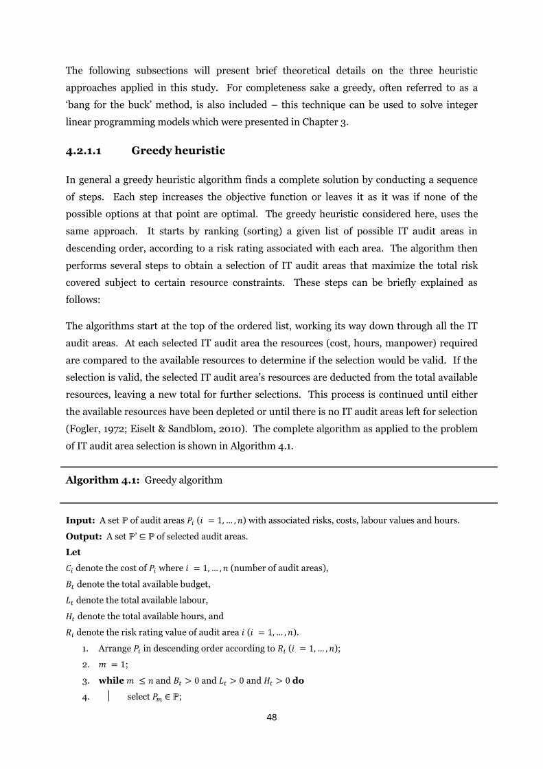
48

The following subsections will present brief theoretical details on the three heuristic

approaches applied in this study. For completeness sake a greedy, often referred to as a

„bang for the buck‟ method, is also included – this technique can be used to solve integer

linear programming models which were presented in Chapter 3.

4.2.1.1 Greedy heuristic

In general a greedy heuristic algorithm finds a complete solution by conducting a sequence

of steps. Each step increases the objective function or leaves it as it was if none of the

possible options at that point are optimal. The greedy heuristic considered here, uses the

same approach. It starts by ranking (sorting) a given list of possible IT audit areas in

descending order, according to a risk rating associated with each area. The algorithm then

performs several steps to obtain a selection of IT audit areas that maximize the total risk

covered subject to certain resource constraints. These steps can be briefly explained as

follows:

The algorithms start at the top of the ordered list, working its way down through all the IT

audit areas. At each selected IT audit area the resources (cost, hours, manpower) required

are compared to the available resources to determine if the selection would be valid. If the

selection is valid, the selected IT audit area‟s resources are deducted from the total available

resources, leaving a new total for further selections. This process is continued until either

the available resources have been depleted or until there is no IT audit areas left for selection

(Fogler, 1972; Eiselt & Sandblom, 2010). The complete algorithm as applied to the problem

of IT audit area selection is shown in Algorithm 4.1.

Algorithm 4.1: Greedy algorithm

Input: A set ℙ of audit areas ( ) with associated risks, costs, labour values and hours.

Output: A set ℙ‟ ⊆ ℙ of selected audit areas.

Let

denote the cost of where (number of audit areas),

denote the total available budget,

denote the total available labour,

denote the total available hours, and

denote the risk rating value of audit area ( ).

1. Arrange in descending order according to ( );

2. ;

3. while and and and do

4. select ℙ;

49

5. , and ;

6. ℙ‟ ← ;

7. ;

8. end

The greedy heuristic presented here is a simple and easy to use heuristic that simply selects

from the top of the ordered list. Fogler (1972) proposed an improvement to this simple

heuristic, which was also considered in this study. The next section details the suggested

improvement.

4.2.1.2 Improved greedy heuristic

The improved greedy heuristic presented by Fogler (1972) was the result of a relative

efficiency test conducted on a ranking technique for capital budgeting problems. The

improved algorithm follows the same steps as the simple greedy algorithm presented in the

previous section, with the only difference being the value used to rank (sort) the projects.

Instead of using the net present value to rank capital projects, a profitability index is

calculated for each project as follows

(4.1)

where:

denotes the profitability index, where ;

is the present value of project , where ; and

denotes the cash outlay for project , within the time period , where

and

The calculated profitability index is then used to rank the projects in descending order. This

technique can now be applied to the IT audit area selection problem by substituting the

appropriate variables into the capital budgeting problem. Algorithm 4.2 presents the

detailed improved greedy algorithm for the IT audit area selection problem. It should be

noted again that the only difference between the greedy and improved greedy algorithm is

the way the ordered list is constructed.

50

Algorithm 4.2: Improved greedy algorithm

Input: A set ℙ of audit areas ( ) with associated risks, costs, manpower values and hours.

Output: A set ℙ‟ ⊆ ℙ of selected audit areas.

Let

denote the total available budget,

denote the total available manpower,

denote the total available hours,

denote the cost of where (number of audit areas),

denote the required hours to audit area , where

denote the required manpower to audit area , where

denote the risk rating value of audit area ( )

1. for do

2.

3. end

4. Arrange in descending order according to ( );

5. ;

6. while and and and do

7. select ℙ;

8. , and ;

9. ℙ‟ ← ;

10. ;

11. end

4.2.1.3 ‘Greedy and swap’ heuristic to solve integer programming

problems

An integer programming model (presented in Chapter 3) is one of the alternatives

considered as a solution for the IT audit area selection problem. These types of models are

usually solved by exact techniques such as the branch-and-bound technique. However, exact

methods may not always be able to solve a given integer linear programming problem within

a reasonable time frame. For this reason heuristic techniques may be used to find a

reasonably good solution quickly. A greedy and swap heuristic, sometimes called „bang for

the buck‟ method, will be presented in this section. It should be noted that this heuristic was

not implemented in the final DSS developed in this research project. The integer

programming models used in the DSS were solved using the branch-and-bound technique.

51

The greedy and swap heuristic can be summarized as follows:

A „value per weight‟ ratio is computed for each decision variable. This can be done by

dividing each variable‟s contribution to the objective function by the coefficients in the

constraint. The variables are then ranked in non-increasing order using these ratios. Once

an ordered list of variables has been constructed, all values are set to zero. The algorithm

then increases the values of variables one by one, starting with the highest rank, as long as

resources are available. As soon as the availability of resources is exceeded, the current

solution and the associated objective function value is taken as the initial solution. The

second phase of the algorithm then raises an arbitrarily chosen variable from zero to one (a

variable entering the solution) and at the same time decreasing another arbitrarily chosen

variable from one to zero (variable that leaves the solution). If this swap is feasible and

increases the value of the objective function, it becomes the new solution. The procedure will

terminate when all feasible pairwise exchanges result in decreases of the value of the

objective function.

A complete worked example of the greedy and swap heuristic for solving an integer linear

programming model can be found in Eiselt & Sandblom (2010).

It should be noted that this heuristic may result in poor solutions. Eiselt & Sandblom (2010)

present a numerical example, showing that poor answers may be obtained in certain cases.

4.2.2 Evolutionary heuristic method

Evolutionary or genetic algorithms are heuristic techniques based on the principle of

evolution. This means that these types of algorithms mimic processes in biological

reproduction by applying a „survival of the fittest‟ principal. These techniques are usually

used to solve models which cannot be optimized in any other way and differs from other

techniques in its implementation and design. They can be applied to very difficult

optimization problems, but being such powerful methods also has its setbacks when it comes

to producing an optimal solution. Because evolutionary algorithms are best suited for use in

problems with non-smooth objective functions, they permit more flexibility than the linear

programming model presented in Chapter 3. This flexibility, however, comes at a price of

not finding an optimal solution, with the reason for this being that evolutionary heuristics do

not make assumptions about the nature of a problem‟s objective function. (Powell & Baker,

2010)

A typical evolutionary genetic algorithm follows a sequence of stages. These stages

correspond to generations in a biological population and within each generation a

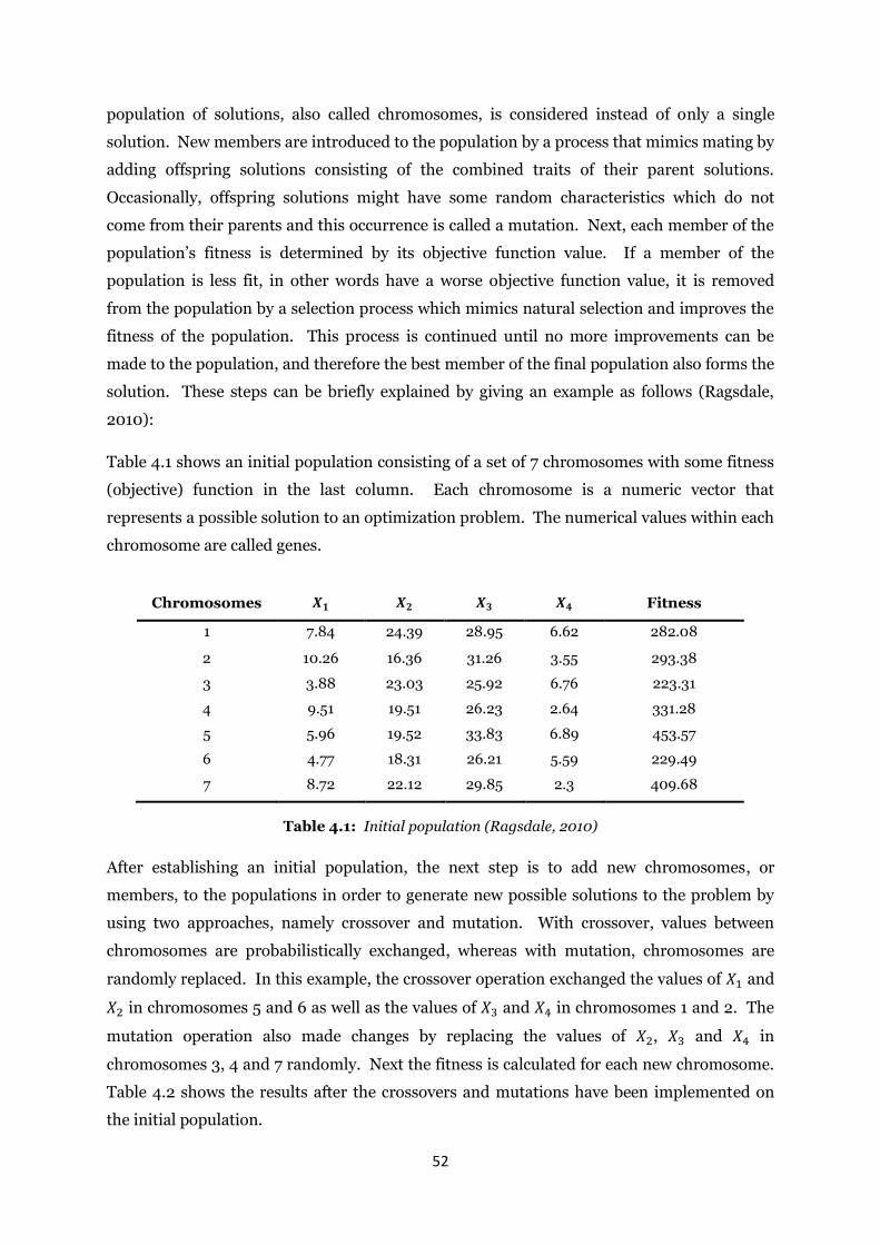
52

population of solutions, also called chromosomes, is considered instead of only a single

solution. New members are introduced to the population by a process that mimics mating by

adding offspring solutions consisting of the combined traits of their parent solutions.

Occasionally, offspring solutions might have some random characteristics which do not

come from their parents and this occurrence is called a mutation. Next, each member of the

population‟s fitness is determined by its objective function value. If a member of the

population is less fit, in other words have a worse objective function value, it is removed

from the population by a selection process which mimics natural selection and improves the

fitness of the population. This process is continued until no more improvements can be

made to the population, and therefore the best member of the final population also forms the

solution. These steps can be briefly explained by giving an example as follows (Ragsdale,

2010):

Table 4.1 shows an initial population consisting of a set of 7 chromosomes with some fitness

(objective) function in the last column. Each chromosome is a numeric vector that

represents a possible solution to an optimization problem. The numerical values within each

chromosome are called genes.

Chromosomes Fitness

1 7.84 24.39 28.95 6.62 282.08

2 10.26 16.36 31.26 3.55 293.38

3 3.88 23.03 25.92 6.76 223.31

4 9.51 19.51 26.23 2.64 331.28

5 5.96 19.52 33.83 6.89 453.57

6 4.77 18.31 26.21 5.59 229.49

7 8.72 22.12 29.85 2.3 409.68

Table 4.1: Initial population (Ragsdale, 2010)

After establishing an initial population, the next step is to add new chromosomes, or

members, to the populations in order to generate new possible solutions to the problem by

using two approaches, namely crossover and mutation. With crossover, values between

chromosomes are probabilistically exchanged, whereas with mutation, chromosomes are

randomly replaced. In this example, the crossover operation exchanged the values of and

in chromosomes 5 and 6 as well as the values of and in chromosomes 1 and 2. The

mutation operation also made changes by replacing the values of , and in

chromosomes 3, 4 and 7 randomly. Next the fitness is calculated for each new chromosome.

Table 4.2 shows the results after the crossovers and mutations have been implemented on

the initial population.

53

Chromosomes Fitness

1 7.84 24.39 31.26 3.55 334.28

2 10.26 16.36 28.95 6.62 227.04

3 3.88 19.75 25.92 6.76 301.44

4 9.51 19.51 32.23 2.64 495.52

5 4.77 18.31 33.83 6.89 332.38

6 5.96 19.52 26.21 5.59 444.21

7 8.72 22.12 29.85 4.60 478.93

Table 4.2: Crossover and Mutation (Ragsdale, 2010)

After applying crossover and mutation and calculating the fitness of each new chromosome,

the new fitness is compared to the corresponding chromosome‟s fitness in the initial

population. On each comparison, only the chromosome which is most fit survives and is

therefore used in the next population. Table 4.3 shows the new computed population, which

will form the new initial population for the next iteration of the described process.

Chromosomes Fitness

1 7.84 24.39 31.26 3.55 334.28

2 10.26 16.36 31.26 3.55 293.38

3 3.88 19.75 25.92 6.76 301.44

4 9.51 19.51 32.23 2.64 495.52

5 5.96 19.52 33.83 6.89 453.57

6 5.96 19.52 26.21 5.59 444.21

7 8.72 22.12 29.85 4.60 478.93

Table 4.3: New Population (Ragsdale, 2010)

Note that several procedures exist to implement crossover, mutation and survival of the

fittest and that this example only served as a general explanation of how the genetic

algorithm works.

As mentioned, the genetic algorithm is different from other optimization methods. To see

how it differs from classical, derivative-based optimization algorithms, consider Table 4.4

below, which shows the two main differences that separate these algorithms (MathWorks,

2013).

Crossover

Crossover

Mutation

54

Classical Algorithm Genetic Algorithm

At each iteration, a single point

is created. The sequence of

points approach an optimal

solution.

At each iteration, a population

of points are generated. The

best point in the population

approaches an optimal

solution.

Selects the next point in the

sequence by deterministic

computation.

Selects the next population by

computation, which uses

random number generators.

Table 4.4: Differences between classical and genetic algorithms

These advantages also cause the genetic algorithm to work better when certain types of

constraints are present in a mathematical optimization model. One such type of constraint is

when dependencies are added among items in such a way that the selection of one item will

influence the value added to the objective function by another item. When applied to a

capital budgeting problem, these constraints can be added to a model by using non-smooth

functions, which make the model inappropriate to solve using a linear programming model.

The genetic algorithm, however, is perfect for these situations, but because these algorithms

are less efficient when constraints are present, one change is needed in order to implement

dependencies among items. Instead of adding an explicit dependency constraint, a new term

is added to the objective function. This term is called a penalty function and is subtracted

from the objective function and therefore „penalizes‟ the solution whenever a resource

constraint is violated.

To see how penalty functions can be used in the selection of IT audit areas, consider the

following simplistic example which uses the same approach used for capital budgeting

problems described above. Table 4.5 shows 3 IT audit areas that can be selected for audit,

with associated risk and cost values:

Audit Area Risk

Rating Cost

Logical Access 0.83 500

Administrator Rights 0.95 400

Backup and Recovery Review 0.60 100

Table 4.5: List of IT audit areas

55

Consider the following mathematical formulation for the information presented in Table 4.5

above

(4.2)

(4.3)

(4.4)

A penalty function can be implemented to penalize the solution whenever the cost constraint

is violated. This penalty function must be assigned a penalty value ( which is subtracted

from the objective value whenever the cost constraint is violated. It is important that the

penalty value is large enough to show a substantial disincentive in the objective value.

Therefore, a penalty value of 99 was selected to be subtracted from the objective value if the

cost constraint is violated.

Let represent the cost to audit Backup and Recovery Review. Suppose a dependency

exists among Logical Access ( and Backup and Recovery Review ( in such a way that

if Logical Access is selected for audit , it changes from its original value of to a

new value of . Using Microsoft Excel‟s “IF” notation, a penalty function can now be

added to the model where . The model can be formulated as

follows

(4.5)

(4.6)

where:

- ;

- ; and

- .

The genetic algorithm can now be applied to this model.

4.2.3 Motivation for selecting heuristics to be included in DSS

For this study, only the greedy, improved greedy and evolutionary heuristics were

implemented, together with a mixed integer linear programming model, to select IT audit

areas.

The goal of the DSS is to select the best combination of IT audit areas, based on a risk rating,

to audit. In order to select a combination of areas among a group of areas, requires binary 0-

1 selection algorithms used in capital budgeting and portfolio investment problems as

56

explained in Chapter 3. To test the performance and efficiency of several algorithms used in

capital budgeting problems and applied to this study, a combination of heuristic methods,

which do not necessarily yield the optimal value, and a linear programming method, which

always gives the optimal solution, is used. Of the heuristic methods described in this section,

the simple greedy heuristic, improved greedy heuristic and the evolutionary algorithm are

implemented in the DSS.

The simple greedy heuristic method was chosen because of its simplicity, speed and that it

requires little computing resources. Being a greedy algorithm, it does not always deliver an

optimal solution, but it is effective for acquiring a good solution fast.

The improved greedy heuristic algorithm was chosen for the same reason as the simple

greedy heuristic. The fact that the objective value weights used for sorting in this algorithm,

are computed in a different way, adds a new dimension to the greedy method which might

yield a different ranking order of audit areas. This may lead to the improved greedy heuristic

yielding a different and hopefully a better solution.

Evolutionary heuristics work well with complex search spaces. This motivates the

implementation of this algorithm in the DSS, taking into consideration that logical operators

will be used to add restrictions for including and excluding selected IT audit areas from the

audit, as well as adding dependencies among the IT audit areas. In doing so, the search

space may become complex to solve and might lead to the evolutionary algorithm producing

better solutions than the greedy methods described above. This is particularly appropriate in

this study where the selection of one area may cause the risk rating of another audit area to

change.

The greedy and swap method is not implemented in the DSS due to the complexity of

creating a programmatic model to solve problems by using the „swap‟ procedure described in

Section 4.2.1.3.

Chapter 3, Section 3.2 described a linear programming method for solving binary 0-1 integer

problems. This method, despite of not being a heuristic method, is also implemented in the

DSS‟s. The implementation is due to several reasons. First of all, the linear programming

method ensures that all possible solutions are generated in order to choose an optimal

solution. Linear programming methods always produce an optimal solution and are

therefore desirable to implement in the DSS. The linear programming method is also robust

and therefore produces the same solution on every run for a specific problem which

increases the quality of this method.

57

4.3 Chapter summary

The aim of this chapter was to introduce and explain the heuristic algorithms studied for the

selection of IT audit areas to audit. It also included the reasons for implementing or not

implementing these heuristic algorithms in the DSS.

Chapter 5 will present an introductory overview of DSS‟s as well as an overview of the DSS

developed in this study.

58

Chapter 5

5. DSS for selecting IT audit areas

5.1 Introduction

Chapter 4 presented and explained the heuristic algorithms considered in this study and

clarified which heuristics were selected for implementation in the DSS. This chapter will

focus on providing sufficient background information and literature on DSS‟s and will

present the DSS developed for the study.

A brief theoretical background on DSS‟s will be presented, after which the actual DSS that

was developed will be will be presented and explained. Finally, the different decision rules

(or requirements) implemented in the DSS will be discussed by using appropriate examples

to show how these requirements were implemented in the DSS for the respective

mathematical techniques.

5.2 Decision support systems

In the past few years the business environment has been changing, which makes operation

within this environment more complex. These changes are caused by factors such as

globalization, customer demands, changing markets, new and improved technologies and

societal changes. Except for these factors, reduced budgets and increased pressures from top

management to perform and increase profits also cause problems. In some cases the

problems created by a changing business environment also generates opportunities, for

example globalization creates opportunities because it allows business to be conducted on a

global scale which might save money and up sales, but on the other hand, globalization leads

to more competition. In order to counter the problems or pressures, organizations need to

respond. Different actions can be used to respond to these factors which are unique to each

business environment and situation. Most of these actions require computerized support

which can be enabled by computerized DSS‟s (Turban et al., 2010).

The remainder of this theoretical overview of DSS‟s is mainly based on the work of Turban et

al. (2010). Some of the work and figures are therefore quoted from his source without

referencing it continuously.

One of the goals of computerized decision support is helping organizations to increase their

current performance in order to reach their desired performance as the organization‟s

59

objectives, goals, mission and strategy express it. Figure 5.1 below gives a schematic

presentation of the three components described, namely business pressures, organizational

response to these pressures and the computerized support which enhance organizations‟

response actions.

Figure 5.1: Business Pressures-Responses-Support Model

Computerized systems have moved from applications that monitor activities and process

transactions to applications that facilitate problem analysis with much of the activities being

done by web-based technologies. In today‟s business world managers have to make

important business decisions. In order to make these decisions they use information

systems, business intelligence tools and the web to assist them. These tools and technologies

play a key role in modern management decision making, and there are several reasons why

computerized systems can be used to support decision making, which are summarized in

Table 5.1.

Capability Description

Speed Computer can perform many computations and evaluate thousands of

alternatives very quickly at a low cost

Communication and

collaboration

Improves the communication and collaboration among group members

situated in different locations by using web-based tools

Group member

productivity Software optimization tools increase productivity of group members

Data management

Improves data management because computers can search, store and

transmit data in different databases very fast and economically while

keeping the data secure and transparent

Organization

Responses

Decisions and

Support

Globalization

Customer demand

Government regulations

Market conditions

Competition

Etc.

Strategy

Partners’ collaboration

Real-time response

Agility

Increased productivity

New vendors

New business models

Etc.

Analysis

Predictions

Decisions

Integrated

Computerized

decision support

Business

intelligence

Business

Environmental Factors

Pressures

Opportunities

60

Management of

gigantic data

warehouses

Computers provide great storage capabilities for large amounts of digital

information, which can then be very speedily accessed, mined and searched

Quality support

Improves the quality of decisions made due to computer systems‟ capability

to performing complex simulations, check many possible scenarios and

assess diverse impacts quickly and economically

Agility support Decision support technologies allow organizations to adapt quickly to rapidly

changing environments and allow for good decisions to be made quickly

Processing and storing

information

Computerized systems are not limited to accessing and processing large

amounts of stored information as people are and therefore overcome the

cognitive limits that people have

Web usage

The internet, web servers and tools enable decision makers to collaborate

with remote partners, provide access to large amounts of information across

the world and intelligent search tools lower the cost of and time to find

information managers need

Overall support Wireless technology allows decision makers to access, interpret and analyze

information and data anywhere and anytime.

Table 5.1: Reasons for using computerized DSS’s

The earliest definition for the concept of DSS‟s can be found in Gorry & Scott-Morton (1971)

who defined it as “interactive computer-based systems, which help decision makers utilize

data and models to solve unstructured problems”. Keen & Scott-Morton (1978) went on to

extend this concept by stating that “decision support systems couple the intellectual

resources of individuals with the capabilities of the computer to improve the quality of

decisions. It is a computer-based support system for management decision makers who

deal with semistructured problems”. Note that the term „DSS‟ can have different meanings

to different people and that no general definition exists. It can therefore be seen as an

umbrella term to describe any computerized system which aid organizations in decision

making. The scope of this term can also be narrowed down so that the term can be referred

to as the process of building custom applications for problems that are unstructured and

semistructured, or to the DSS being the application itself.

Except for the concept of DSS‟s being an umbrella term and also being referred to as the

application building process or the application itself, another important aspect of this

concept is its architecture, which comprises of several components (Druzdzel & Flynn,

2007). The first component is data management, which is concerned with storing data

relevant to the situation, as well as adding capabilities to access internal and external data. A

second component is model management, which delivers the analytical capabilities of the

61

system by manipulating the data related to a specific situation. These models can either be

customized or standard. The third component only exists in some systems and is known as

the knowledge component. Another vital component is the users. The users communicate

directly with the system by using a user interface which forms the fifth and final component

of a DSS‟s architecture. In order to fully understand the concept of DSS‟s, it should also be

known that many types of DSS‟s exist with the two major types being model-oriented and

data-oriented DSS‟s (Power & Sharda, 2007). Model-oriented DSS‟s are based on

quantitative models which recommend a solution to a problem, whereas data-oriented DSS‟s

allow for reporting and query functionalities.

DSS‟s usually include models. A model is a “simplified representation, or abstraction of

reality” and is simplified because problems in reality are too complex to explain. With

DSS‟s, analysis is performed on these models of reality and not on reality itself. Models

represent problems and each problem has a degree of abstraction which is used to classify

the model into four groups: iconic, analogue, mental and mathematical models. Iconic

models are small physical replications of original systems and are the least abstract of all

models. Analogue models on the other hand only behave like the real systems but have a

different shape. Mental models are usually used when mostly qualitative factors play a role

in making decisions and are subjective descriptions of individuals‟ thinking process about

situations. The final type of models, mathematical models, are more abstract than all other

models and are usually used in situations where relationships in systems are too complex to

represent using the other models. Analysis in DSS‟s is usually executed numerically using

quantitative models, such as mathematical models, which comprise of three variables: a

decision, an uncontrollable and a result. Relationships exist among these three variables.

(Turban et al., 2008)

Decision making is a process which consists of four major phases: intelligence, design, choice

and implementation phase. Figure 5.2 shows the process followed in computer-based

decision making. The first phase in the decision making process is intelligence. This phase

involves examining a situation in order to identify and define the problem while also

establishing the problem ownership. The second phase is design and involves constructing a

model for the problem identified in the first phase. To construct a model, the reality is

simplified by making assumptions, and relationships among variables are conveyed. This

phase also involves validation of the model and identification of evaluation criteria for all

possible solutions. After phase two the process enters the choice phase. Here a solution is

chosen and tested to see if the solution is feasible. A feasible solution leads to the fourth

phase called implementation. If the implementation is successful, the problem is solved.

62

However, if the implementation fails, the process can return to any of the previous three

phases. (Turban et al., 2008)

Figure 5.2: Decision making process

As mentioned earlier, no general definition for DSS‟s exist. This means that no standard set

of characteristics and capabilities exist for DSS‟s. Figure 5.3 presents a set of 14 ideal

capabilities and characteristics DSS‟s consist of.

Reality Intelligence Phase

Organization objectives

Search and scanning procedures

Data collection

Problem identification

Problem ownership

Problem classification

Problem statement

Design Phase

Formulate a model

Set criteria for choice

Search for alternatives

Predict and measure outcomes

Choice Phase

Solution to the model

Sensitivity analysis

Selection of the best (good)

alternative(s)

Plan for implementation

Implementation

of solution

Simplification

Assumptions

Validation of the model

Verification, testing of proposed

solution

Success

Failure

Problem Statement

Alternatives

63

Figure 5.3: Ideal characteristics and capabilities of a DSS

In order to understand the characteristics and capabilities presented in Figure 5.3, a brief

explanation for each of the 14 characteristics, as numbered in Figure 5.3 above, is presented

below.

1. Supports decision makers in semistructured and unstructured situations to solve

problems that cannot be solved using standard quantitative methods and tools by

combining computerized information and human judgment.

2. Supports all levels of management.

Decision Support Systems

Semistructured or unstructured

problems Support

managers at all levels

Support individuals and

groups

Interdependent or sequencial

decisions

Support intelligence

design, choice, and

implementation

Support a variety of decision

processes and styles

Adaptable and flexible

Interactive, ease of use

Effectiveness and efficiency

Humans control the process

Ease of development by

end users

Modelling and analysis

Data access

Stand-alone, integration, and

web-based

1

2

3

4

5

6

7

8

9

10

11

12

13

14

64

3. Supports individual decision making as well as groups consisting of several

individuals from different departments or organizations through virtual teams and

collaborative web tools.

4. Supports decisions that are interdependent and sequential.

5. Support is given in all phases of the decision making process.

6. Supports a wide range of decision making styles and processes.

7. DSS‟s are flexible and can easily be modified to solve other problems.

8. DSS‟s can be made more effective by implementing a natural language interactive

human-machine interface, as well as strong graphical capabilities and web-based

interfaces.

9. Deployment of DSS‟s might slow down the problem solving process, but at the same

time it improves the effectiveness of decision making by making better decisions.

10. Supports the decision maker in all steps of the decision making process rather than

replacing the decision maker.

11. Simplifies system development for end users.

12. Models are used in analysis to experiment with different strategies and

configurations, which sets DSS‟s apart from other management information systems.

13. Provides access to various data sources.

14. DSS‟s can be used by individuals as a stand-alone tool, it can be integrated with other

systems or distributed using the web.

The operation, implementation and designing process of a DSS is dependent on the type of

DSS involved. Most of these different types fit into a classification model created by Power

(2001) which includes five categories: model-driven, data-driven, document-driven,

communication-driven and group, and knowledge-driven DSS‟s.

Model-driven DSS‟s give emphasis to the access and manipulation of models, such as

financial, optimization and representational models. These systems are developed around

one or more model which includes activities such as the formulation, maintenance and

management of models as well as what-if analysis. Therefore, the main goal of these systems

is to optimize an objective or objectives by using models. This category uses quantitative

tools to provide basic level functionality. Data and parameters are used to analyse situations,

but model driven DSS‟s do not require large databases as they are not data intensive (Power,

2001).

In data-driven models, structured data including time-series of internal and external data

can be accessed, manipulated, processed and analysed by using computerized techniques.

The main purpose of these systems is to process the data into information to represent to

65

decision makers. The data is stored on simple file systems and accessed by using retrieval

and query tools, which provide the basic level functionality. Online analytical processing, on

the other hand, provides the highest level of functionality and decision support linked to

analysing large amounts of historical data. DSS‟s developed in online analytical processing

and data mining software systems usually form part of this category. Also, the prominence

of using mathematical models in this category of systems is minimal. (Mohemad et al.,

2010; Power, 2001)

Document-driven DSS‟s allow integration of document databases and processing

technologies so that decision makers can access, retrieve, manage and analyse these

unstructured documents. These type of systems put little emphasis on the utilization of

mathematical models. Search engines and the web acts as a helping tool and provides access

to large databases of documents such as text documents, images, sounds and videos.

Essentially all DSS‟s that are text based, fall into this category such as Knowledge

Management Systems. (Mohemad et al., 2010; Power, 2001)

A fourth category is knowledge-driven DSS‟s which use inference engines to understand a

problem. These systems solve a problem domain and suggest actions in order to aid decision

makers. This decision making process is automated by using rules. Methods such as rule-

based, statistical based, object-based and logic-based methods help to store knowledge about

a certain domain in a reusable form. All artificial intelligence-based DSS‟s fall into this

category. (Mohemad et al., 2010)

Lastly, communication-driven and group DSS‟s allow interactive communication with the

system by geographically dispersed decision makers through networking technology. This

category essentially includes all kinds of DSS‟s where group work is present. (Mohemad et

al., 2010)

Note that except for these five categories, two or more of these categories can also be

combined to form a hybrid category called compound DSS‟s.

A DSS is made up of several components. These components integrate with each other and

include a database management subsystem, a model management subsystem, a user-

interface subsystem and a knowledge-based management subsystem. Figure 5.4 shows a

schematic view of the general structure of a DSS and its components.

66

Figure 5.4: DSS - schematic view.

The database management subsystem contains all the data used in the decision making

process and can be interconnected with a data warehouse, which is a source of relevant

decision making data. This data is stored in a database which is managed by a database

management system (DBMS). The model management subsystem on the other hand, is a

software package that holds all the quantitative models used by the system and which

provide analytical capabilities and software management. The model management system

includes modelling languages that can be utilized to build custom models and can also be

connected to models stored externally. The third component is the user-interface

management subsystem which acts as a communication channel between the user and the

DSS, wherein the user is considered part of the system. One of the most consistent graphical

user interfaces used in DSS‟s is web browsers, but for locally used DSS‟s a similar consistency

in user interfaces is given by spread sheets. The last component is a knowledge-based

management subsystem which can act independently or support any of the other

subsystems. This component can be interconnected with the knowledge repository of a

corporation which may be accessed through a web server. Also, it is not compulsory for a

DSS to have a knowledge-based management subsystem, but if it does exist, it provides

intelligence in the other three components.

The DSS developed in this study optimizes an objective (maximizing the risk) using different

mathematical techniques and can therefore be categorized as a model-driven DSS. In the

next section, the DSS that was developed will be presented. The different types of decision

Other computer-based

systems

Internet, intranet,

extranet

Data

management

Model

management External models

Knowledge-based

subsystems

User interface

Manager (user) Organizational

Knowledge Base

ERP/POS

Legacy

Web, etc.

Data: external

and/or internal

67

rules (or constraints) implemented will be explained as well as how these decision rules were

implemented for each of the mathematical techniques used in the DSS.

5.3 DSS development

The DSS for selecting IT audit areas to audit was created by developing a desktop application

that integrates with Microsoft Excel Solver. The system and all of its models were

programmed in C# and VB (Visual Basic) using Microsoft Visual Studio Ultimate 2012 and

Microsoft Excel 2010 Macro Designer respectively. A CD containing the developed DSS for

selecting IT audit areas to audit and the dataset used in this study is included with the

dissertation. The system requirements for the developed DSS can be found in Appendix A,

Section A.1.

The DSS developed in this study receives as input the IT audit area details from a Microsoft

Excel file. This Excel file contains a specific number of sheets, each with a predetermined

structure and layout, as well as a few pre-programmed VB macros needed to link the

information in the Excel file with the DSS. These macros also make it possible to use

Microsoft Excel‟s Solver function efficiently and effectively from within the DSS.

The user is expected to select and open this Excel file from within the DSS. The data

contained in this file can then be used by one of 4 available methods. As mentioned in

Chapter 4, Section 4.2.3, the four different approaches included in this system is the greedy

heuristic, improved greedy heuristic, 0-1 binary model and evolutionary heuristic.

Each of these approaches can analyse the data input by using one of two options. The first is

called grouped analysis, where a group of IT audit areas can be created consisting of a

combination of IT audit areas (e.g. A group called Systems group can be created which

contain the IT audit areas: Financial Systems, Financial Systems Interfaces and

Engineering Systems). The second option is normal analysis, where no groups of IT audit

areas are created and each IT audit area is considered on its own.

For each of these analysis options, either no decision rules or several different decision rules

can be added. The decision rules allow the user to add constraints to the mathematical

techniques in order to restrict the IT audit area selection. Although thousands of

combinations of decision rules can be built in, only a finite number of decision rules were

built into the DSS in this study. Therefore, a selection of decision rules was made and only

those rules are included. The selection of decision rules to include is based on

correspondence with the audit manager who provided the data, and is also the most common

cases that occur. For grouped analysis, the decision rules that were added are include groups

68

of areas (include specific groups or a number of IT audit areas within a group) and exclude

groups of areas (exclude specific groups or IT audit areas within a group). For normal

analysis, the decision rules that were added are include areas (include specific IT audit

areas), exclude areas (exclude specific IT audit areas), dependencies (add dependencies

among IT audit areas) and include/exclude multiple IT audit areas from sub lists (include or

exclude a certain number of IT audit areas within a sub list of IT audit areas). Figure 5.5

below shows the high level structure of the DSS as described above.

Input of IT audit area details from Excel file

Normal analysis

Grouped analysis

Include areas

Exclude areas

Dependencies

Include group of areas

Exclude group of areas

Include/Exclude multiple IT audit

areas

Analysis

Binary 0-1 model

Evolutionary model

Improved greedy heuristic

Greedy heuristic

Figure 5.5: High level structure of the DSS

The remainder of this chapter is dedicated to explaining the normal and grouped analysis,

and the different decision rules that exist in the DSS for each of these analysis options.

5.3.1 Normal analysis

In Section 5.3, four different types of rules were presented that can be added when normal

analysis is used. These rules include: include areas, exclude areas, include/exclude multiple

areas from sub lists and dependencies. The next few paragraphs will explain each of these

decision rules in more detail and describe why and how they were implemented in the DSS.

69

5.3.1.1 Include areas

When IT audit plans are compiled it is often necessary to include specific management

requirements into the audit plan. This means that normal selection procedures, usually

based on risk ratings, are bypassed and the inclusion of specific audit areas becomes

mandatory. For example, management might want the following four IT audit areas to be

included in the audit plan: Human Resources Systems Interfaces, Financial Systems,

Logical Access and Engineering systems. To ensure that these areas are included in the final

selection, decision rules (constraints) are added to force the mathematical technique used to

select these areas during the selection process. It is important to note that the four selection

models in the DSS differ in terms of how they handle or enforce these decision rules.

0-1 Binary model and evolutionary heuristic:

The 0-1 binary model and the evolutionary heuristic are both binary selection models and to

enforce the inclusion of specific audit areas, a simple logical condition (see Section 3.3.4) can

be implemented.

For example:

Let: If audit area is selected ( (5.1)

otherwise (5.2)

Suppose that the inclusion of two IT audit areas, Logical Access (audit area number 1) and

Change Control (audit area number 4) is mandatory. Consider Table 5.2 below which

presents a short list of available IT audit areas.

Audit Area

Logical Access

Administrator Rights

Backup and Recovery Review

Change Control

Business Continuity

Disaster Recovery

Human Resources


Table 5.2: IT audit areas to include

70

The following two constraints will accomplish this:

= (5.3)

= (5.4)

Greedy heuristic and improved greedy heuristic:

The greedy heuristic and improved greedy heuristic handle the inclusion of IT audit areas in

a different manner. Each IT audit area that must be included in the audit plan should be

selected from the list of IT audit areas and removed from the list before selection on the

remaining IT audit areas can be performed.

As an example consider Table 5.3 which presents a short list of available IT audit areas with

their associated risk ratings, cost, manpower requirements and hours required to perform

the audit.

Audit Area Risk

Rating Cost

Man-power

Hours

Logical Access 0.83 32550 3 175

Administrator Rights 0.95 16182 1 87

Backup and Recovery Review 0.60 32550 6 175

Change Control 0.45 65100 4 350

Business Continuity 0.80 95025 3 525

Disaster Recovery 0.20 32550 4 175

Human Resources 0.50 31675 5 175

Table 5.3: List of IT audit areas available for selection

If the areas Change Control and Logical Access have to be included, both heuristics will

simply find them in the list and remove them from the list. The total risk rating, cost,

manpower and hours available will be adjusted accordingly and a new list with the remaining

5 IT audit areas will then be created. The two heuristics will then proceed to select from the

new list according to the specific heuristic‟s rules.

It should be noted that the same approach (removing areas from the initial list) can in some

of the scenarios also be applied to the 0-1 binary model and the evolutionary heuristic. The

objective is however to apply the models and not to manipulate the input data. For the

greedy and improved greedy heuristics there is no other suitable option than to pre-select (or

pre-exclude) some of the areas and remove them from the initial dataset. The manipulation

of the input dataset and the application of the mathematical models will again be highlighted

in Chapter 6 where the empirical experiments are discussed.

71

5.3.1.2 Exclude areas

Similar to the inclusion of specific areas, management may decide to exclude specific IT

audit areas from an IT audit plan. This implies that they should not be considered for the IT

audit plan.


These two models will implement again a simple logical condition to handle the exclusion of

areas. To exclude the two IT audit areas, Logical access (audit area number 1) and Change

Control (audit area number 4), the following two constraints are added:

= (5.5)

= (5.6)


The IT audit areas that must be excluded is simply removed from the initial list of available

IT audit areas.

5.3.1.3 Include/exclude multiple IT audit areas from sub lists

To include and exclude areas described above can easily be extended to include or exclude a

specific number of IT audit areas from a shorter sub-list of available IT audit areas.


The following constraints serve as examples of how this was implemented in the 0-1 binary

model and evolutionary heuristic

∑

(select exactly areas) (5.7)

∑

(select at least areas) (5.8)

∑

(select at most areas) (5.9)

72


The sub-list will be treated as an initial list where (or at least or at most ) will be selected

from, with values of resources adjusted accordingly. The applicable IT audit areas will then

be removed from the main list and selection can then resume from this new main list.

5.3.1.4 Dependencies

IT audit areas are often linked together and performing an audit on one area may impact

another area. This implies that the audit of a specific IT audit area is dependent on whether

an audit is conducted in another IT audit area. There are two basic dependencies that were

built into the DSS. A normal dependency refers to selecting an IT audit area based on

whether another one was selected or not. It can also refer to either selecting or not selecting

an IT audit area based on whether another one was selected (this scenario is not considered

for this study, although a DSS resolution thereof is presented below). Secondly, a risk

dependency means that the risk rating of an IT audit area will change depending on whether

another IT audit area was chosen or not. These two dependencies will be discussed briefly in

the next few paragraphs.

5.3.1.4.1 Normal dependencies

Consider the following two related IT audit areas: Disaster Recovery (audit area number 6)

and Business Continuity (audit area number 5).


Suppose that a decision was taken that Disaster Recovery should be included in the IT audit

plan if Business Continuity was chosen for inclusion. This would result in the following

constraint in the 0-1 binary model and evolutionary heuristic

(5.10)

If there is a choice to select or not select Disaster Recovery when Business Continuity was

selected, the constraint can be changed to

(5.11)


In the case where one area should be selected if the other one was selected, the heuristics will

proceed as normal and as soon as one of the linked areas is selected, the other one will

73

immediately be selected subject to availability of resources. If there is a choice to select or

not select the one when the other one is selected, the heuristics will proceed in their normal

manner – if one area is selected it will keep working through the list and it may or may not

select the other one, depending on resources.

5.3.1.4.2 Risk dependencies

Every IT audit area has an associated risk rating which represents the threat posed by an

individual area if it is not audited. Different IT audit areas are often related and the auditing

of one area may influence the risk rating of another area. For example, if the IT audit area

Disaster Recovery is audited, the risk posed by the IT audit area Backup and Recovery

Review will decrease because of related aspects between the two areas. This means that the

risk rating of the IT audit area Backup and Recovery Review will change (decrease) because

of the selection of the IT audit area Disaster Recovery for inclusion in the IT audit plan.

There is therefore a risk dependency between the two IT audit areas. It should be noted that

the result of an audit effects how the risk rating of a dependent area will change. In some

cases the risk rating may increase and not decrease e.g. when the results of the Disaster

Recovery audit is bad, it will have a negative influence on related IT audit areas. This study

deals with the construction of an IT audit plan (before the outcome of a specific audit is

known) and therefore only decreasing risk ratings were considered.

Consider the following risk dependency example. If Disaster Recovery (audit area number

6) is selected for inclusion in the IT audit plan, the risk rating for Backup and Recovery

Review (audit area number 3) will decrease from an initial rating of 0.60 to 0.20. This was

dealt with as follows by the two mathematical techniques.


A new, additional, IT audit area has to be added to the list of available IT audit areas. This

new area (audit area number 8) is a replica of the old Backup and Recovery Review area

except for the risk rating which is now 0.20 – see Table 5.4 below.

74

Audit Area Risk

Rating Cost

Man-power

Hours









Table 5.4: List of IT audit areas after adding risk dependency

Two additional constraints are now needed to provide for the changing of the risk rating,

depending on the selection or no selection of the Disaster Recovery area

(5.12)

(5.13)

These two constraints have the following effect:

If Disaster Recovery is selected ( ), then the original Backup and Recovery

Review area with a risk rating of 0.60 cannot be selected ( ); and the new

Backup and Recovery Review area with a risk rating of 0.20 can either be selected or

not selected ( ).

If Disaster Recovery is not selected ( ), then the original Backup and Recovery

Review area with a risk rating of 0.60 can either be selected or not selected (

); and the new Backup and Recovery project with a risk rating of 0.20 cannot

be selected ( )

The net effect of a risk dependency in these mathematical techniques is twofold. First, the

list of available IT audit areas are expanded – a new IT audit area has to be added for each

risk dependency. If there are many risk dependencies, it means that the list of available IT

audit areas will become very long and may add to the complexity of selecting suitable areas

for inclusion in the IT audit plan. Secondly, for every risk dependency two additional logical

constraints have to be added to the model. This may have an impact on the complexity and

time to solve the model.

75


A new, additional IT audit area will be added to the list of available IT audit areas for

selection. As with the 0-1 binary model and evolutionary heuristic, this new IT audit area

(audit area number 8) is an exact replica of the old Backup and Recovery Review area, but

has a new risk rating of 0.20 (refer to Table 5.4 above).

The heuristics will proceed in their normal manner until they find Disaster Recovery and

will either select, or not select it, subject to resource availability. This could have one of the

following effects:

If Disaster Recovery is selected, then the original Backup and Recovery Review area

will simply be removed from the list, which leaves the new Backup and Recovery

Review area with a risk rating of 0.20 in the list and available for selection.

If Disaster Recovery is not selected, then the new Backup and Recovery area with a

risk rating of 0.20 will be removed from the list, which leaves the original Backup

and Recovery Review area with a risk rating of 0.60 in the list and available for

selection.

With these heuristics, when risk dependencies are added, the list of IT audit areas available

for selection also expands. As with the 0-1 binary model and evolutionary heuristic a new IT

audit area is added to the list of available IT audit areas for each risk dependency that exists.

This causes the list of available IT audit areas to become very long and might make the

selection of suitable areas to include in the IT audit plan more complex.

5.3.2 Grouped analysis

Section 5.3 presented two different decision rules that can be added when grouped analysis

is used. These rules are: include groups of areas and exclude groups of areas. The remainder

of this chapter will present more detailed explanations for each of these decision rules and

will describe why and how they were implemented in the DSS.

5.3.2.1 Include groups of areas

When management have specific requirements, these requirements need to be included in

the IT audit plan when it is compiled. When grouped analysis is used, management might

want to include one of two things. Firstly, the specific management requirements might

state that a group of IT audit areas should be included. For example, management might

want to include the Systems group containing 6 IT audit areas. Secondly, the requirements

can be to include the best possible number of IT audit areas within a specific group. For

76

example, management may want to include the best 3 IT audit areas out of the 6 IT audit

areas in the Systems group. As with normal analysis, decision rules (constraints) can be

added to ensure that the mathematical techniques used include these areas in the final

selection. Note that with grouped analysis, as with normal analysis, the four selection

approaches also differ in the way that they handle and enforce these decision rules.


As mentioned in Section 5.3.1.1, both the 0-1 binary model and evolutionary heuristic are

binary selection models and can therefore handle the inclusion of a specific group of IT audit

areas by implementing a simple logical condition.

For example:

Let: If audit area is selected ( (5.14)

otherwise (5.15)

Suppose that IT audit areas Logical Access (audit area number 1), Administration Rights

(audit area number 2), Change Control (audit area number 4) and Disaster Recovery (audit

area number 6) form a group called Access Control and that the inclusion of this group is

mandatory. Consider Table 5.5 below which presents a short list of available IT audit areas.

Audit Area

Logical Access

Administrator Rights


Change Control

Business Continuity

Disaster Recovery

Human Resources


Table 5.5: IT audit areas to include

This inclusion can be accomplished by adding the following constraint

= (5.16)

The following constraints serve as an example of how exactly, at least or at most 3 IT audit

areas within Access Control can be included

(select exactly 3 areas) (5.17)

77

(select at least 3 areas) (5.18)

(select at most 3 areas) (5.19)


The greedy heuristic and improved greedy heuristic handle the inclusion of IT audit areas in

a group differently. To include a group of IT audit areas in the audit plan, each IT audit area

in the group should be selected from the list of IT audit areas and removed from the list

before selection on the remaining IT audit areas can be performed.

As an example, consider Table 5.6, which presents a short list of available IT audit areas with

their associated risk ratings, cost, manpower requirements, and hours required to perform

the audit, with the group Access Control, as used in the 0-1 binary model and evolutionary

heuristic example above, to be included.

Audit Area Risk

Rating Cost

Man-power

Hours









Both heuristics will simply find the IT audit areas Logical Access (audit area number 1),

Administration Rights (audit area number 2), Change Control (audit area number 4) and

Disaster Recovery (audit area number 6) that are in the group Access Control, and remove

them from the list while adjusting the total risk rating, cost, manpower and hours available

accordingly. This will create a new list with the remaining 3 IT audit areas. The two

heuristics will then proceed to select from the new list according to the specific heuristic‟s

rules.

To include exactly, less than or more than IT audit areas in a group, the list of IT audit

areas should first be sorted in descending order of the risk rating. Consider Table 5.7 below

showing a sorted representation of Table 5.6 presented above.

78

Audit Area Risk

Rating Cost

Man-power

Hours









Both heuristics will select exactly, less than or more than IT audit areas out of the IT audit

areas Logical Access (audit area number 2), Administration Rights (audit area number 1),

Change Control (audit area number 6) and Disaster Recovery (audit area number 7). They

will then remove the chosen areas from the list of IT audit areas, and adjust the total risk

rating, cost, manpower and hours available accordingly. A new list with the remaining IT

audit areas will then be created, from which selection on the remaining areas can be

performed by the specific heuristic.

It is important to note that if not all of the areas in the group Access Control can be included

according to the constraints given, the algorithms will not remove any of these areas from

the initial list, and no adjustments will be made to the to the risk rating, cost, manpower or

hours available.

5.3.2.2 Exclude groups of areas

As with inclusion of groups or a number of IT audit areas within a group, management might

decide to exclude a specific group of IT audit areas or a number of IT audit areas within a

specific group from an IT audit plan. These areas should therefore not be considered for the

IT audit plan.


The 0-1 binary model and evolutionary heuristic handle the exclusion of a group or specific

number of IT audit areas within a group by implementing a simple logical condition. To

exclude Access Control implies that Logical Access (audit area number 1), Administration

Rights (audit area number 2), Change Control (audit area number 4) and Disaster Recovery

(audit area number 6) should be excluded from the IT audit plan and can be accomplished by

adding the following constraint

79

= (5.20)


To exclude a group of IT audit areas, both heuristics will simply remove the IT audit areas in

the group from the initial list of available areas. When specific IT audit areas within a group

must be excluded, the heuristics will again remove the areas from the initial list of available

areas. In this case, the removed IT audit areas will not exist in the group anymore.

5.4 Chapter summary

In this chapter an introductory overview of DSS‟s was presented. The DSS that was

developed in this study was also presented to gain a good understanding of how the DSS is

structured. Two types of analysis, normal and grouped analysis used in the DSS, were

explained. For each of these types, the different decision rules implemented in the DSS were

discussed as well as how each mathematical technique implements them.

Chapter 6 will present the empirical experiments conducted with the different decision rules.

80

Chapter 6

6. Empirical experiments and results

6.1 Introduction

In the previous chapter, the linear programming model and the different heuristics that were

used in this study were presented and explained. The heuristics include the greedy,

improved greedy and evolutionary heuristic algorithms. In this chapter, a detailed

discussion will be given on the data collected, the different experiments conducted and the

results obtained from these experiments.

The chapter starts out with an explanation of the data set used after which the comparative

criteria for comparing experiment results will be presented. Next, the different experiments

will be presented and explained, and finally, the chapter will be concluded with a general

discussion and recommendations based on the experiment results.

6.2 Data collection and processing

The data used in this study was collected from a large well-established organisation in order

to obtain trustworthy real world data. The organisation in question is a large multi-billion

dollar Australian company with over 3500 IT users. The company is a geographically

dispersed utility and supply essential services to over 2 million customers. The organisation

set up a list of 41 possible IT audit areas that can be included in their annual IT audit plan.

Each IT audit area in this list has 5 data fields. For each of these data fields, the data was

given directly by the organisation. The 5 data fields provided by the organisation are as

follows:

Risk rating: Each IT audit area has a risk rating assigned to it which represents the

risk the area poses to the organization. Risk is presented as a value between 0

(lowest risk) and 1 (highest risk) or similarly between 0% and 100%. For example, if

the IT audit area Logical Access has a risk rating of 0.83, it means that Logical Access

has a high risk of 0.83 (or 83%) on a scale of 0-1 (or 0-100%).

Cost: Each IT audit area has a cost assigned to it which shows how much it will cost

the organization to perform an audit on the specific area. If the IT audit area Logical

Access has a cost of 4 300, it means that it will cost the organization 4 300 Australian

dollars to audit Logical Access.

81

Manpower: When an IT audit area is audited, the audit is conducted by a certain

number of people. Therefore, each IT audit area has a manpower assigned to it which

represents the number of people needed to audit each specific area. As an example, if

IT audit area Logical Access has a manpower of 3, it means that 3 people are needed

to audit Logical Access.

Hours: Represents the number of hours it will take to audit an IT audit area.

Consider an IT audit area Logical Access with an hour‟s value of 48. This means that

it will take 48 hours to audit Logical Access.

Dependencies: Dependencies may exist among two or more IT audit areas in such a

way that if one area is audited, it has an effect on another IT audit area‟s risk rating.

The audit area Administrator Rights in Table 6.1 below is dependent on another

audit area, namely Logical Access. If the area Logical Access is audited,

Administrator Rights’ risk rating changes from the original risk rating of 0.95 to a

new risk rating of 0.75. In some cases a single audit area can also have more than

one dependent area (See Section 5.3.1.4 for further explanation).

Table 6.1 shows the dataset used in this study.

Audit Area Risk

Rating Cost

Man-power

Hours Dependencies

# Areas

Risk Rating

1 Logical Access 0.83 32550 3 175 - -

2 Administrator Rights 0.95 16182 1 87 Logical Access

0.75

3 Physical Access 0.55 16182 2 87 - -

4 Change Control 0.45 65100 4 350 - -

5 Business Continuity 0.80 95025 3 525

Disaster Recovery, Backup and Recovery Review

0.50

6 Disaster Recovery 0.20 32550 4 175 Backup and Recovery Review

0.10

7 Human Resources 0.50 31675 5 175 - -

8 Human Resources Systems Interfaces

0.75 32550 3 175 Human Resources

0.25

9 Financial Systems 0.30 95025 6 525 - -

10 Financial Systems Interfaces

0.82 32550 4 175 - -

11 Engineering Systems 0.40 95025 5 525 - -

12 Antivirus Management

0.33 31675 2 175 - -

13 Software License Fees Review

0.15 16182 1 87 - -

14 Incident and Problem Management

0.73 31675 3 175 - -

82

15 IT Capacity Management

0.35 16182 4 87 - -

16 IT Risk Management 0.90 23711 3 131 - IT

Governance 0.75

17 Electronic Fund Transfers

1.00 32550 5 175 - -

18 IT Security Awareness

0.80 63350 3 350 - Logical

Access 0.75

19 Problem Management

0.38 65100 4 350 - -

20 Patch Management 0.28 7783 2 43 - -

21 Network Security Baseline Review

0.25 31675 4 175 - -

22 Network Penetration Testing

0.89 63350 6 350 - -

23

IT Governance (New Systems Implementation Policies and Procedures)

1.00 65100 5 350 - -

24 IT Hardware and Software Standards

0.10 31675 2 175 - -

25 Backup and Recovery Review

0.60 32550 6 175 - -

26 ICT Legislation Compliance Review

0.79 15747 3 87 - IT

Governance 0.55

27 King lll, or Aus Equivalent, Compliance Review

0.81 15747 2 87 - -

28 User Training on IT Systems

0.29 24366 1 131 - -

29 E-Approval of Contracts

0.91 7783 1 43 - -

30 Software Inventory Management

0.28 16182 2 87 - -

31 Hardware Inventory Management

0.63 15747 2 87 - -

32 CICS or Any Operating System Environment

0.22 63350 6 350 - -

33 Data Base Management

0.21 63350 7 350 - -

34 Data Integrity 0.86 192675 7 525

- Logical Access, Financial Systems Interfaces

0.60

35 Privacy of Customer Records and Information

0.92 31675 3 175 - -

36 Use of Illegal or Non Standard Software

0.52 32550 1 175

- Change Control, IT Hardware and Software Standards, Software Inventory Management

0.25

37 Time and Attendance 0.51 63350 5 350 - -

38 Mobile Applications 0.74 63350 7 350 - -

83

39 Business Fit or IT Architecture

0.58 31675 3 175 - IT

Governance 0.40

40 Impact of BYO Devices on Security

0.73 32550 4 175

- Procurement and Control of Mobile Equipment (iPhones, Laptops)

0.68

41

Procurement and Control of Mobile Equipment (iPhones, Laptops)

0.74 32550 4 175 - -

Table 6.1: IT audit area dataset

6.3 Comparative criteria

The goal of the experiments is to investigate which of the heuristic methods or mathematical

model perform the best when certain circumstances exist. These circumstances relate to real

world problems or constraints that usually exist when selecting IT audit areas for inclusion

in an IT audit plan. To reach this goal, a number of experiments were set up to test certain

measureable values, after which the results of these experiments were then compared in

terms of certain criteria to see which model or heuristic performs best under which

circumstances. The criteria that will be used to compare the experiment results are as

follows:

6.3.1 Risk coverage

As mentioned in Section 6.2 and shown in Table 6.1, each IT audit area in the dataset has a

risk value assigned to it. This risk rating represents a figure showing how important it is for

an IT audit area to be audited or, in other words, the need to be audited. In this study a

maximization approach was used in order to maximize the amount of risk covered by the

combination of IT audit areas selected by the mathematical model and heuristics. If the total

computed risk value is low, it means that the combination of IT audit areas selected by the

algorithm is poor, whereas a high total risk value means the algorithm covered a high

amount of risk by the specific combination of IT audit areas it selected.

The maximum risk covered by the mathematical model and heuristics will be compared in

the form of a percentage, which represents the percentage of risk covered out of the total

possible coverable risk.

84

6.3.2 Resource utilization

Only a limited amount of funds, manpower and hours are available for conducting the IT

audits. An additional goal of each heuristic and the mathematical model, will be to utilize as

much of these available resources as possible. If this is not the case, resources would have

been wasted and this will also have a declining effect on the total computed risk value

mentioned in the previous paragraph. Taking this into consideration it can be stated that the

resources that will be needed to conduct the selected IT audit, must be as close as possible or

equal to the total available resources in order for an algorithm to perform well.

The mathematical model and heuristics will be compared in terms of their resource

utilization to determine which of them use the available resources most effectively. The

resource utilization will be calculated as a percentage of the total available funds, hours and

manpower used. Resource utilization will be calculated for each individual resource used,

namely funds, hours and manpower as

(6.1)

6.3.3 Model formulation complexity

To measure the complexity of formulating the mathematical model and heuristics for each

experiment, two quantifiable measures, namely programmatic complexity and model

complexity, were developed.

Programmatic complexity is a score-based variable and measures how difficult it is to

programmatically implement the heuristics or model in the DSS under certain conditions.

The effect of this complexity has already been mentioned in Chapter 4, Section 4.2.3 where

the „greedy and swap‟ heuristic method proved to be too difficult in specific instances to

programmatically implement in the DSS. Therefore, for every experiment, the 0-1 binary

model and each of the heuristics will be given a score between 0 and 10, with 0 being very

simple and 10 extremely difficult to programmatically implement.

The programmatic complexity plays a very significant role, as some of the constraints added

in the different experiments may be very basic formulations. However, the programming of

these constraints and implementation thereof in a DSS is often not that straightforward and

may cause a number of programming complexities.

Model complexity measures how difficult it is to set up and solve the mathematical model

and heuristics when a specific decision rule exists. While some decision rules can be

85

implemented easily (without complicating the manner in which a problem is solved), others

can cause the model or heuristics to become so complex that in some cases the problem

becomes intractable. As with programmatic complexity, the mathematical model and

heuristics for each experiment will be given a score between 0 and 10.

The model formulation complexity is calculated as a percentage where 0% represents the

easiest and 100% the most complex as

(6.2)

6.3.4 Baseline computation time deviation

The computation time before a mathematical model or heuristic produces an answer, needs

to be considered. This time depends on the complexity and number of operations that need

to be executed, as well as the ability of the specific model or heuristic to solve a certain

scenario. Another important factor is the processing capacity of the computer used. The

experiments might therefore have different computation times if conducted using another

computer than those documented in this study. However, the times will still show the same

results for the heuristics and mathematical model relative to each other. In saying that, the

number and type of constraints added will also affect the time each heuristic and the

mathematical model takes before finding the best possible solution. Therefore, the

computation time for solving the IT audit area selection problem without adding any

additional constraints will be used as baseline to measure how much the addition of

constraints in each experiment, increase or decrease (or deviates from) the baseline

computation time for the mathematical model and each heuristic. The computation time for

the mathematical model and each heuristic in Experiment 1 (to be explained in Section

6.4.1), will therefore be used as the baseline computation time.

To measure how much a specific set of constraints deviates from the baseline computation

time, a percentage is calculated. This is the percentage of the baseline computation time that

the specific set of constraints adds on top of the baseline. As an example, suppose the

baseline computation time for the 0-1 binary model is 1 second. After adding 3 additional

constraints to the model, the computation time becomes 1.5 seconds. This means the 3

constraints increased the baseline computation time by 0.5 seconds, which is a 50% increase

(deviation) and in effect also means the model is 50% slower than the baseline. Note that a

decrease in computation time will be presented as a negative percentage in the experiment

86

results. A negative percentage therefore represents an improvement (faster computation

time).

In this study, the computation time measurement starts as soon as the user clicks on the

“Solve” button. This sets off a programmatic stopwatch timer which keeps on running until

the best possible answer is found, at which point the stopwatch is stopped.

6.4 The experiments

Overall 7 experiments were conducted. The first 6 experiments relate to normal analysis

(when no groups consisting of several IT audit areas exist), as explained in Chapter 5 Section

5.3.1. The last experiment relates to group analysis (when a number of groups exist, each

consisting of several IT audit areas), as explained in Chapter 5 Section 5.3.2.

The main goal of the experiments is to see which of the different heuristics or mathematical

model presented in Chapters 3 and 4 performs the best when several different decision rules

exist, as presented in Chapter 5, Section 5.3. Therefore, an experiment was created for each

of the decision rules that exist and is outlined in Table 6.2 below. Each of these experiments

will be discussed in more detail later on in Section 6.4.1-6.4.7.

Experiments

Experiment 1 No decision rules

Experiment 2 Exclude specific IT audit areas

Experiment 3 Include specific IT audit areas

Experiment 4 Include/Exclude multiple IT audit

areas

Experiment 5 Normal dependent areas

Experiment 6 Risk dependent areas

Experiment 7 Grouped analysis

Table 6.2: Experiments conducted

Each experiment produces results for each of the heuristics and mathematical model used.

The results relate to 5 measures which will be used to calculate the values for each of the

comparative criteria in Section 6.3. The 5 measures are as follows:

Computation time: Measures the time taken to compute results.

Number of areas selected: Measures the number of IT audit areas selected for

inclusion in the audit plan.

87

Risk covered: The goal is to maximize the risk covered by all the IT audit areas

selected for inclusion in the IT audit plan. Therefore the sum of the risk ratings of all

the IT audit areas selected for inclusion will be used to compare the four techniques

and determine which of them covers the most risk.

Funds not utilized: With this measure, the model and heuristics will be compared to

see which of them utilizes the total available budget most effectively.

Hours not utilized: For each of the four techniques, it provides an indication of the

amount of hours out of the total number of hours available not utilized efficiently.

Manpower not utilized: This measure will be used to compare the model and

heuristics to see which of them utilized the total available manpower most

effectively.

The remainder of this chapter is dedicated to presenting each experiment conducted and

results obtained, followed by a summarized overview of all the experiment results.

6.4.1 Experiment 1 (Normal analysis) – No decision rules

Experiment description: In experiment 1, there are no rules or requirements and the 0-1

binary model and heuristics simply take the given data set and try to choose as many IT audit

areas as possible to cover as much as possible risk. This is the simplest scenario and as

mentioned in Section 6.3.4, the computation time of this experiment will also be used as a

baseline for all subsequent experiments. Therefore, the baseline computation time deviation

in this experiment is 0% for all techniques. Table 6.3 below presents the results. Here, each

measure in which the techniques performed best is highlighted. This will henceforth be true

for all subsequent experiment results. Also, the graphical representation of the results in this

experiment and all experiments to follow is depicted in two separate figures. This is to

separate the model formulation complexity (which is not a result produced by the DSS) from

the risk coverage and resource utilization results (which are produced by the DSS). Due to

the scale used to graphically represent the DSS results, the values of the baseline

computation time deviation is too small to depict on the same graph as the risk coverage and

resource utilization. Therefore it will only be available in the results table of each

experiment.

88

Experiment Results

Measures Greedy

Heuristic

Improved

Greedy

Heuristic

0-1 Binary

Model

Evolutionary

Heuristic

Computation time (Milliseconds) 0.001 0.001 1436 73205

Number of areas selected 26 29 30 30

Risk covered (Total Rating) 19.71 19.64 20.29 20.29

Funds not utilized (Rands) 230808 228770 229645 229645

Hours not utilized (Hours) 35 37 37 37

Manpower not utilized (People) 3 9 0 0

Comparative Criteria Results

Criteria Greedy

Heuristic

Improved

Greedy

Heuristic

0-1 Binary

Model

Evolutionary

Heuristic

Total Risk coverage 81.95% 81.66% 84.37% 84.37%

Funds utilized effectively 82.51% 82.67% 82.60% 82.60%

Hours utilized effectively 99.36% 99.32% 99.32% 99.32%

Manpower utilized effectively 96.88% 90.63% 100% 100%

Model formulation

complexity 5.00% 6.00% 7.50% 8.50%

Baseline computation time

deviation 0% 0% 0% 0%

Table 6.3: Experiment 1 – Comparative criteria results

The programmatic complexity for all four approaches is fairly simple because no decision

rules exist and therefore it makes the programming straightforward. However, the 0-1

binary model and evolutionary model is slightly more difficult to program, because the DSS

for these techniques interfaces with Microsoft Excel‟s Solver and requires more specialized

coding. Due to this a programmatic complexity rating of 1, 1.2, 1.5 and 1.7 out of 10 was

given to the greedy heuristic, improved greedy heuristic, 0-1 binary model an evolutionary

heuristic respectively (as discussed in Section 6.3.3). In terms of the model complexity, no

decision rules are added and therefore there is nothing in this experiment to measure this

against (as discussed in Section 6.3.3). Therefore, a score of 0 out of 10 was given to every

technique. The total model formulation complexity percentages, as in Table 6.3, were

calculated by adding up the programmatic and model complexity for each technique and

dividing it by 20.

Note that the same calculation method is used to calculate the total model formulation

complexity percentages in all subsequent experiments.

89

The final complexity calculations in Table 6.3 can be graphically presented as in Figure 6.1

below.

Figure 6.1: Experiment 1 - Model formulation complexity

Figure 6.2 below presents the risk coverage and resource utilization efficiency graphically.

Figure 6.2: Experiment 1 – DSS results

0.00%

5.00%

10.00%

15.00%

20.00%

25.00%

Model formulation complexity

Greedy Heuristic

Improved GreedyHeuristic

0-1 Binary Model

Evolutionary Heuristic

74.00%75.00%76.00%77.00%78.00%79.00%80.00%81.00%82.00%83.00%84.00%85.00%86.00%87.00%88.00%89.00%90.00%91.00%92.00%93.00%94.00%95.00%96.00%97.00%98.00%99.00%

100.00%

Total Riskcoverage

Fundsutilized

effectively

Hoursutilized

effectively

Manpowerutilized

effectively

Greedy Heuristic


0-1 Binary Model


90

In the simplest scenario where there are no rules and IT audit areas are simply chosen, the

evolutionary heuristic and 0-1 binary model fared the best in terms of the risk covered.

Although the greedy and improved greedy heuristic did not cover the highest risk, they both

are very similar in utilizing the available resources. While the improved greedy heuristic

performed best in utilizing the available funds, the greedy heuristic is better than all

techniques when it comes to utilizing hours efficiently. Manpower was best utilized by the

evolutionary heuristic.

The results indicated that in the case where there are no rules or requirements, any one of

the approaches may be used. One may select the 0-1 binary model or evolutionary heuristic

which both cover the highest risk. On the other hand one may instead select the greedy

heuristic as this technique has the lowest complexity.

6.4.2 Experiment 2 (Normal analysis) – Exclude specific IT audit

areas

Experiment description: Experiment 2 deals with the case where specific IT audit areas

should be excluded. This scenario often occurs when management, for example, decides to

exclude audit areas, or when they do not have the specific expertise to conduct the audit at

that stage. Audit areas that were recently audited are also candidates for exclusion. It was

decided, for testing purposes, to exclude 7 areas in this experiment. These 7 areas were

randomly chosen from the dataset presented in Table 6.1 using Excel's random number

function. The areas selected by Excel were areas number 9, 13, 14, 18, 23, 30 and 39 in Table

6.1 (the dataset). The requirement to exclude IT audit areas causes changes to the 0-1 binary

model and evolutionary heuristic, because an additional constraint had to be added. With

regards to the other heuristics, the areas that should be excluded are simply removed from

the dataset, after which the heuristics are applied as in Experiment 1. The detail of the

additional constraint is as follows:

Let be the set of excluded areas. The additional constraint is then formulated as

∑

(6.3)

(Only for the binary 0-1 model and evolutionary algorithm)

It should be noted that the 0-1 binary model and the evolutionary heuristic may be handled

in the same way as the greedy algorithms, i.e. removing the areas to be excluded from the

dataset and then performing experiment 1 again with the reduced dataset. This option,

however, was not preferred and not tested due to the following reasons:

91

The objective is to evaluate capital budgeting models for IT audit area selection and

not to manipulate the dataset. The manipulation of the dataset for the greedy and

improved greedy heuristic forms part of the heuristic;

The DSS is designed to formulate models and perform selections based on rule

specification of a user and not to manipulate the input dataset; and

The additional constraint generated here forms the basis (programmatically) for

other requirements, where a minimum or maximum number of areas have to be

excluded. See for example experiment 4 in Section 6.4.4. In this case it is impossible

to remove them before a solution has been obtained.

Table 6.4 below shows the results obtained.

Experiment Results

Measures Greedy

Heuristic

Improved

Greedy

Heuristic

0-1 Binary

Model

Evolutionary

Heuristic








Criteria Greedy

Heuristic

Improved

Greedy

Heuristic

0-1 Binary

Model

Evolutionary

Heuristic




Manpower utilized effectively 96.88% 98.96% 100% 100%

Model formulation

complexity 7.50% 8.50% 20.00% 21.00%


deviation 0.00% 0.00% -2.72% 0.16%


Table 6.4 shows that the programmatic complexity of all four techniques has increased when

IT audit areas are excluded, as opposed to experiment 1, where no decision rules were added.

This is due to decision rules or constraints that must be added. The 0-1 binary model and

92

evolutionary heuristic is almost two times more difficult to program than the other

heuristics. This is because a constraint must be constructed in the DSS for the 0-1 binary

model and evolutionary heuristic, which is not easy to program. On the other hand, to

exclude IT audit areas using the greedy (which has the lowest model formulation complexity)

and improved greedy heuristic, requires a small addition of fairly simple code. Therefore the

greedy heuristic, improved greedy heuristic, 0-1 binary model and evolutionary heuristic

were assigned programmatic complexity scores of 1.5, 1.7, 3 and 3.2 out of 10 respectively.

To exclude IT audit areas is very easily implemented in the greedy and improved greedy

heuristic and the model complexity for both received a score of 0 out of 10. To set up the

models for the 0-1 binary model and evolutionary heuristic, an additional constraint must be

added which increase their model formulation complexity. They were both assigned a score

of 1 out of 10. The model formulation complexity scores given in Table 6.4 are graphically

presented in Figure 6.3 below.


A graphical representation of the DSS results (as in Table 6.4) can be seen in Figure 6.4.

0.00%

5.00%

10.00%

15.00%

20.00%

25.00%


Greedy Heuristic


0-1 Binary Model


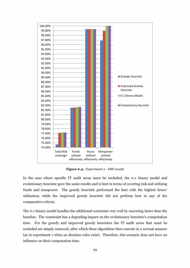
93

Figure 6.4: Experiment 2 - DSS results

In the case where specific IT audit areas must be excluded, the 0-1 binary model and

evolutionary heuristic gave the same results and is best in terms of covering risk and utilizing

funds and manpower. The greedy heuristic performed the best with the highest hours‟

utilization, while the improved greedy heuristic did not perform best in any of the

comparative criteria.

The 0-1 binary model handles the additional constraint very well by executing faster than the

baseline. The constraint has a degrading impact on the evolutionary heuristic‟s computation

time. For the greedy and improved greedy heuristics the IT audit areas that must be

excluded are simply removed, after which these algorithms then execute in a normal manner

(as in experiment 1 when no decision rules exist). Therefore, this scenario does not have an

influence on their computation time.

74.00%

75.00%

76.00%

77.00%

78.00%

79.00%

80.00%

81.00%

82.00%

83.00%

84.00%

85.00%

86.00%

87.00%

88.00%

89.00%

90.00%

91.00%

92.00%

93.00%

94.00%

95.00%

96.00%

97.00%

98.00%

99.00%

100.00%

Total Riskcoverage

Fundsutilized

effectively

Hoursutilized

effectively

Manpowerutilized

effectively

Greedy Heuristic


0-1 Binary Model


94

It should be noted that the figures for the resources may be different, even if the number of

areas selected are the same (as in Table 6.4). This is due to the fact that different techniques

may select different areas, but the same number of areas.

To outline the above, when IT audit areas must be excluded, the 0-1 binary model and

evolutionary heuristics may be considered. The 0-1 binary model and evolutionary heuristic

produce the exact same results, but the binary model has a lower model formulation

complexity and a negative deviation from the baseline computation time. The greedy

heuristic should only be considered when the objective is to utilize the available hours

effectively.

6.4.3 Experiment 3 (Normal analysis) – Include specific IT audit

areas

Experiment description: This experiment describes a scenario where specific IT audit

areas must be included for audit. This is often the case when specific management

requirements exist, when statutory requirements exist which state that an area must be

audited, when an area was audited long ago or when there was a significant recent change

and management wants to audit it. The experiment will use the same set of 7 IT audit areas

used in experiment 2 (where specific IT audit areas were excluded). These are areas number

9, 13, 14, 18, 23, 30 and 39 in Table 6.1 (the dataset). As in experiment 2, the inclusion of IT

audit areas cause changes to the 0-1 binary model and evolutionary heuristic, because an

additional constraint had to be added. For the other two heuristics, the IT audit areas that

should be included are chosen immediately, after which they are removed from the dataset.

The greedy and improved greedy heuristics are then simply applied as in experiment 1

(where no decision rules were added). The detail of the additional constraint is as follows:

Let be the set of areas to be included. The additional constraint is then formulated as

∑

(6.4)

(Only for the binary 0-1 model and evolutionary algorithm)

It should once again be noted that for the 0-1 binary model and the evolutionary heuristic

the areas to be included can be selected immediately, then removed from the dataset and

then perform the same experiment as experiment 1 with this new (reduced) dataset. This

option was again not further explored. The reasons for not exploring this option are the

same as explained in experiment 2 (Section 6.4.2).

95

Table 6.5 below presents the experiment results.

Experiment Results

Measures Greedy

Heuristic

Improved

Greedy

Heuristic

0-1 Binary

Model

Evolutionary

Heuristic








Criteria Greedy

Heuristic

Improved

Greedy

Heuristic

0-1 Binary

Model

Evolutionary

Heuristic




Manpower utilized effectively 93.75% 89.58% 96.88% 96.88%

Model formulation

complexity 18.50% 19.50% 20.00% 21.00%


deviation 0.00% 0.00% 0.91% -6.65%


Table 6.5 shows that for the greedy and improved greedy heuristics, the inclusion decision

rule is about twice as complex to program than in experiment 2. Inclusion requires

additional calculations that must be programmed to cater for the actual selection of these

areas in the DSS. The programmatic complexity ratings for the greedy and improved greedy

heuristics are 1.7 and 1.9. The 0-1 binary model and evolutionary heuristic, however, was

assigned the same programmatic complexity score as in experiment 2, where these areas

were excluded. This is because there is no difference in programmatically adding the

constraint to these two techniques when areas are included or excluded. Programmatic

complexity scores of 3 and 3.2 were given to the 0-1 binary model and evolutionary heuristic

respectively. The models of the greedy and improved greedy heuristics are more complex

than that of the 0-1 binary model and evolutionary heuristic. In order to include areas, the

greedy and improved greedy heuristics must first select the areas to include, subject to the

availability of resources, and thus increase their model complexity. A model complexity

96

rating of 2 out of 10 was given for the greedy and improved greedy heuristics. For the 0-1

binary model and evolutionary heuristic, the model complexity is similar to when areas are

excluded. This is because the model is set up in the same way with only a simple change

required in the constraint. Therefore, a model complexity rating of 1 out of 10 was given for

both.

The model formulation complexity presented in Table 6.5 can be graphically depicted as in

Figure 6.5 below.


0.00%

5.00%

10.00%

15.00%

20.00%

25.00%


Greedy Heuristic


0-1 Binary Model


97


When IT audit areas must be included, the techniques give quite different results. Figure 6.5

and Figure 6.6 show that the 0-1 binary model performed best in terms of risk covered and

manpower utilized but was altogether the worst in using funds and hours effectively. The

evolutionary heuristic did the best in using manpower, but selected fewer areas than the 0-1

binary model and covered a lower risk. Even though the improved greedy heuristic chose the

same number of areas as the evolutionary heuristic, the combination of areas selected proved

to be weaker because it covered a lower risk. It also did not perform best in any criteria. On

the other hand, the greedy heuristic covered the lowest risk but utilized both funds and hours

most efficiently. It also has the smallest model formulation complexity.

In Table 6.5, one can see the 0-1 binary model has a small positive baseline computation

time deviation. It therefore performs slightly slower than the baseline (as in experiment 1

where no decision rules exist). On the other hand, the evolutionary heuristic performed

much quicker than the baseline, as presented by the negative baseline computation time

deviation. Once again there is no deviation in the baseline computation time for the greedy

and improved greedy heuristics.

74.00%75.00%76.00%77.00%78.00%79.00%80.00%81.00%82.00%83.00%84.00%85.00%86.00%87.00%88.00%89.00%90.00%91.00%92.00%93.00%94.00%95.00%96.00%97.00%98.00%99.00%

100.00%

Total Riskcoverage

Fundsutilized

effectively

Hoursutilized

effectively

Manpowerutilized

effectively

Greedy Heuristic


0-1 Binary Model


98

To summarize, it may be said the 0-1 binary model is the best option when IT audit areas

should be included. If only manpower is taken into account however, the evolutionary

heuristics might also be selected. Although the greedy heuristic is the simplest in this

scenario, it should only be considered in situations where the use of the available hours or

funds is the main goal, due to its low risk coverage and manpower utilization. The improved

greedy heuristic did not perform best in any of the comparative criteria and should therefore

not be considered.

6.4.4 Experiment 4 (Normal analysis) – Include/Exclude a number

of IT audit areas

Experiment description: Experiment 4 describes an extension on experiments 2 and 3.

In experiment 4 it is assumed that a sub-set of areas exist and that an exact number of areas,

or a minimum number of areas, or a maximum number of areas have to be included or

excluded from this pre-defined sub-set. This type of scenario may exist due to the same

reasons explained for experiments 2 and 3. This extension means that for the greedy and

improved greedy heuristics, the sub-set is treated as an initial list of areas to select from.

Once this selection has been made, the sub-set is simply removed from the main dataset and

the heuristics are then applied to the remaining areas in the same manner as in experiment

1. In terms of the 0-1 binary model and evolutionary heuristic, additional constraints have to

be added. These constraints can be formulated as follows:

Let be the subset of areas from which an exact number of areas have to be selected. The

constraint to be added is as follows

∑

(6.5)

where is the number of areas to be selected from and ;

Let be the subset of areas from which at least of areas should be selected. The

constraint then becomes

∑

(6.6)

where is the minimum number of areas to select from and ;

Finally, let be the subset of areas from which at most of areas should be selected. The

additional constraint is then formulated as

99

∑

(6.7)

where is the maximum number of areas to select from and ;

To implement and test these extensions it was decided to populate with the same 7 areas

used in experiment 2 and 3, and and with 7 other areas that were randomly selected

from the main dataset. This random selection was also performed using Excel‟s random

number function. For a value of was selected; for a value of ; and for a

value of . The results for the experiment using these values are presented in Table 6.6

and Figures 6.7 and 6.8.

Experiment Results

Measures Greedy

Heuristic

Improved

Greedy

Heuristic

0-1 Binary

Model

Evolutionary

Heuristic








Criteria Greedy

Heuristic

Improved

Greedy

Heuristic

0-1 Binary

Model

Evolutionary

Heuristic


Funds used effectively 82.58% 82.48% 82.55% 82.68%

Hours used effectively 99.36% 99.34% 99.34% 99.34%

Manpower used effectively 95.83% 81.25% 98.96% 100%

Model formulation

complexity 35.00% 36.00% 35.00% 36.00%


deviation 0.00% 0.00% 1.39% -5.73%


100



34.40%

34.60%

34.80%

35.00%

35.20%

35.40%

35.60%

35.80%

36.00%

36.20%


Greedy Heuristic


0-1 Binary Model


70.00%71.00%72.00%73.00%74.00%75.00%76.00%77.00%78.00%79.00%80.00%81.00%82.00%83.00%84.00%85.00%86.00%87.00%88.00%89.00%90.00%91.00%92.00%93.00%94.00%95.00%96.00%97.00%98.00%99.00%

100.00%

Total Riskcoverage

Fundsutilized

effectively

Hoursutilized

effectively

Manpowerutilized

effectively

Greedy Heuristic


0-1 Binary Model


101

As experiment 4 is an extension of experiments 2 and 3, the results are also more or less in

line with the results of experiments 2 and 3. The 0-1 binary model still performs the best. It

should be noted, however, that there was a significant increase in the model formulation

complexity. This is due to the programmatic complexity that was increased by adding

additional constraints. Inserting these constraints dynamically into the DSS complicated the

programming to a large degree.

The results from Table 6.6 indicate that it is safe to use the 0-1 binary model for the scenario

described in this section.

6.4.5 Experiment 5 (Normal analysis) – Add normal dependencies

among specific IT audit areas

Experiment description: Experiment 5 deals with the case where two or more IT audit

areas are linked together. This means that if one of the linked IT audit areas is selected, the

other area must also be selected (forced dependency). Audit areas are normally linked when

the areas are closely related or when audit assurance is required for a broader area. For

example, the audit areas Business Continuity and Disaster Recovery are very closely related

and in some instances cover the same risk areas. Therefore it makes sense to audit the

controls of Disaster Recovery at the same time when the area Business Continuity is

audited. In these cases management may instruct their Internal Audit department to select a

specific audit area(s) based on the selection of another one.

The organization who provided the main dataset also specified 11 specific links which are

used in their environment. The 11 links are as follows:

If (Administrator Rights) is selected, then (Logical Access) must also be

selected.

If (Business Continuity) is selected, then (Disaster Recovery) and

(Backup and Recovery Review) must also be selected.

If (Disaster Recovery) is selected, then (Backup and Recovery Review)

must also be selected.

If (Human Resources Systems Interfaces) is selected, then (Human

Resources) must also be selected.

If (IT Risk Management) is selected, then (IT Governance) must also be

selected.

If (IT Security Awareness) is selected, then (Logical Access) must also be

selected.

102

If (ICT Legislation Compliance Review) is selected, then (IT Governance)

must also be selected.

If (Data Integrity) is selected, then (Logical Access) and (Financial

Systems Interfaces) must also be selected.

If (Use of Illegal or Non Standard Software) is selected, then (Change

Control), (IT Hardware and Software Standards) and (Software Inventory

Management) must also be selected.

If (Business Fit or IT Architecture) is selected, then (IT Governance) must

also be selected.

If (Impact of BYO Devices on Security) is selected, then (Procurement and

Control of Mobile Equipment) must also be selected.

All 11 dependencies were implemented in experiment 5. The greedy and improved greedy

heuristics are applied in the same manner as in experiment 1, but as soon as one of the

linked areas is selected, the other area(s) will automatically be selected depending on the

availability of resources. Should the resources not be sufficient to select the linked area(s),

adjustments have to be implemented to reverse the appropriate selections and allocated

resources. This has a major impact on the programmatic complexity of the otherwise simple

and straightforward greedy and improved greedy heuristics. It also makes it very difficult to

set up the models for the greedy and improved greedy heuristics.

For the 0-1 binary model and evolutionary heuristic, an additional constraint has to be added

for each link. As with the other experiments, these additional constraints are fairly simple,

but to incorporate them dynamically into the DSS greatly increases programmatic and model

complexity. The additional constraints for the 0-1 binary model and evolutionary heuristic

can be formulated as follows:

If there is a link between only 2 audit areas (If is selected then must also be selected,

)

and . (6.8)

If one audit area is linked to more than one other audit area, the constraint to be added is:

Let be the set of audit areas that is linked to. and

∑

(6.9)

103

The result for experiment 5 is presented in Table 6.7 and Figures 6.9 and 6.10 below.

Experiment Results

Measures Greedy

Heuristic

Improved

Greedy

Heuristic

0-1 Binary

Model

Evolutionary

Heuristic








Criteria Greedy

Heuristic

Improved

Greedy

Heuristic

0-1 Binary

Model

Evolutionary

Heuristic




Manpower used effectively 100% 95.83% 100% 89.58%

Model formulation

complexity 85.00% 86.00% 62.50% 64.50%


deviation 0.00% 0.00% 32.59% -1.10%



0.00%

10.00%

20.00%

30.00%

40.00%

50.00%

60.00%

70.00%

80.00%

90.00%

100.00%


Greedy Heuristic


0-1 Binary Model


104


The results of experiment 5 once again show that the 0-1 binary model outperforms the other

approaches in most of the criteria. What is of particular interest is the high level of risk

covered and the effective use of funds and manpower. Contrary to expectations it was also

relatively easier to set up the 0-1 binary model than the other techniques. The evolutionary

heuristic required the implementation of penalty functions (for each additional constraint)

while changes to the greedy and improved greedy heuristic algorithms becomes difficult to

implement programmatically.

6.4.6 Experiment 6 (Normal analysis) – Add risk dependencies

among specific IT audit areas

Experiment description: Experiment 6 deals with situations where certain audit areas

are related in such a way that the auditing of one area will influence the risk rating of another

area. For example, the auditing of Business Continuity may influence the risk rating of

Disaster Recovery, as some of the controls audited in Business Continuity also apply to

50.00%

52.00%

54.00%

56.00%

58.00%

60.00%

62.00%

64.00%

66.00%

68.00%

70.00%

72.00%

74.00%

76.00%

78.00%

80.00%

82.00%

84.00%

86.00%

88.00%

90.00%

92.00%

94.00%

96.00%

98.00%

100.00%

Total Riskcoverage

Fundsutilized

effectively

Hoursutilized

effectively

Manpowerutilized

effectively

Greedy Heuristic


0-1 Binary Model


105

Disaster Recovery. This influence may be positive (i.e. positive audit results may reduce the

risk of a related audit area) or it may be negative (i.e. negative audit results may increase the

risk of a related audit area). In this study only positive influences (reduced risk rating for a

related audit area) were considered. For the purpose of this study it is assumed that a new

IT audit plan is constructed. This means that there are no prior audits or audit results that

can have a negative influence on any of the linked audit areas. In experiment 6 it was

therefore assumed that a positive influence (reduced risk ratings) will occur. The DSS can

easily be adapted to provide for a negative influence if necessary.

The scenario described here is an important one and occurs often in the construction of audit

plans where audit areas have to be selected. Although the required changes to the different

solution approaches may sound trivial, the implementation is fairly complicated.

For the greedy and improved greedy heuristics the implementation is as follows:

Suppose audit area 1 (risk rating 0.85) and audit area 2 (risk rating 0.75) is related. If audit

area 1 is selected, the risk rating of audit area 2 will decrease to 0.60. An additional audit

area (risk rating 0.60) is now added to the sorted list of possible audit areas. This

additional audit area represents audit area 2 with a reduced risk rating. The heuristics are

now applied as in experiment 1. If audit area 1 (which is related to audit area 2) is selected,

then the original audit area 2 (risk rating 0.75) is removed from the list and the algorithm

may or may not choose audit area with the reduced risk rating. If audit area 1 is not

selected, the additional audit area , with the reduced risk rating, is removed from the list

and the algorithm may or may not select the original audit area 2. In all cases the resources

must continually be adjusted to reflect the adding and removing of audit areas.

To implement these risk dependency cases in the 0-1 binary model and evolutionary

heuristic, a number of additional constraints and variables need to be added. Consider the

same example as above. An additional audit area is again added to the list of possible audit

areas and the following two constraints are added

(6.10)

(6.11)

where is an additional variable representing the additional audit area .

These constraints will ensure that whenever is selected, cannot be selected and may

or may not be selected. If is not selected the audit area may or may not be selected

while cannot be selected.

106

In cases where there are more than one dependency (i.e. selection of audit area 1 will reduce

the risk rating of audit area 2 and audit area 3), an additional audit area, reflecting the lower

risk ratings for both dependencies as well as additional variables, are added. The constraints

are then adapted to make provision for the multiple dependencies, e.g. for two dependencies

the constraints become

(6.12)

. (6.13)

The organization which provided the data for the study also provided 11 risk dependencies

(see Table 6.1) that occur in their business. These risk dependencies were included in this

experiment and are as follows:

If (Administrator Rights) is selected, the risk rating of (Logical Access) becomes

.

If (Business Continuity) is selected, the risk rating of (Disaster Recovery) and

(Backup and Recovery Review) becomes .

If (Disaster Recovery) is selected, the risk rating of (Backup and Recovery

Review) becomes .

If (Human Resources Systems Interfaces) is selected, the risk rating of (Human

Resources) becomes .

If (IT Risk Management) is selected, the risk rating of (IT Governance)

becomes .

If (IT Security Awareness) is selected, the risk rating of (Logical Access)

becomes .

If (ICT Legislation Compliance Review) is selected, the risk rating of (IT

Governance) becomes .

If (Data Integrity) is selected, the risk rating of (Logical Access) and

(Financial Systems Interfaces) becomes .

If (Use of Illegal or Non Standard Software) is selected, the risk rating of

(Change Control), (IT Hardware and Software Standards) and (Software

Inventory Management) becomes .

If (Business Fit or IT Architecture) is selected, the risk rating of (IT

Governance) becomes .

If (Impact of BYO Devices on Security) is selected, the risk rating of

(Procurement and Control of Mobile Equipment) becomes .

107

Results of the risk dependent audit area experiment are presented in Table 6.8 and Figures

6.11 and 6.12.

Experiment Results

Measures Greedy

Heuristic

Improved

Greedy

Heuristic

0-1 Binary

Model

Evolutionary

Heuristic








Criteria Greedy

Heuristic

Improved

Greedy

Heuristic

0-1 Binary

Model

Evolutionary

Heuristic




Manpower used effectively 94.79% 94.79% 98.96% 100%

Model formulation

complexity 90.00% 91.00% 80.00% 82.00%


deviation 600.00% 1000.00% 67.69% 31.91%

Table 6.8: Experiment 6 – Comparative criteria


74.00%

76.00%

78.00%

80.00%

82.00%

84.00%

86.00%

88.00%

90.00%

92.00%


Greedy Heuristic


0-1 Binary Model


108


The results of this experiment indicated that the model formulation complexity of the models

have increased dramatically. This is due to the programmatic complexity of the greedy and

improved greedy heuristics as well as the constraints and variables for the other two

techniques (as described above). There is no specific approach that outperforms all other

approaches in all areas. If the main criteria is total risk covered, then the 0-1 binary model,

which is also the least complex, should be selected. The greedy heuristic has done well in

terms of the effective use of resources such as funds and hours, but is very complex to

implement programmatically in the DSS. The poor performance of the evolutionary

heuristic is a result of the many penalty functions that had to be added to provide for the

constraints. In large datasets with a large number of risk dependencies the evolutionary

heuristic may perform even worse. The impact of risk dependencies is also reflected in the

baseline computation time deviation, where all techniques are much slower, especially the

greedy and improved greedy heuristics, than when any other decision rules exit.

74.00%

75.00%

76.00%

77.00%

78.00%

79.00%

80.00%

81.00%

82.00%

83.00%

84.00%

85.00%

86.00%

87.00%

88.00%

89.00%

90.00%

91.00%

92.00%

93.00%

94.00%

95.00%

96.00%

97.00%

98.00%

99.00%

100.00%

Total Riskcoverage

Fundsutilized

effectively

Hoursutilized

effectively

Manpowerutilized

effectively

Greedy Heuristic


0-1 Binary Model


109

6.4.7 Experiment 7 (Grouped analysis)

In practice it often happens that audit areas are grouped together and that a complete group

has to be dealt with in a certain way. For example, all financial related audit areas may be

grouped into one group and management may decide that this specific group must be

excluded (e.g. when the group was audited recently) or included (e.g. when the group has not

been audited recently). To evaluate these grouped scenarios, three further experiments were

conducted in the same manner as the experiments already discussed. This was done as

follows:

Experiment 2 was extended to exclude specific groups of audit areas instead of

specific audit areas;

Experiment 3 was extended to include specific groups of audit areas instead of

specific audit areas; and

Experiment 4 was extended to include/exclude a number of audit areas within a

specific group.

In all three cases the constraints and changes required to the heuristics were virtually the

same as in experiments 2 to 4. There were therefore no significant changes in the results of

these “grouped” experiments, and the tables and graphs, which were presented for the first 6

experiments, are therefore omitted.

6.5 General discussion, recommendations and contribution

Section 6.5 will present a general discussion and recommendations following the empirical

experiments and the development of the DSS. First, comments will be made regarding the

application of the techniques in the area of internal auditing. This will be followed by some

remarks pertaining to the development of the DSS.

6.5.1 The use of a mathematical technique to construct an IT audit

plan

Traditionally, audit plans are constructed through discussions and consensus by

stakeholders. These decisions are normally based on a risk rating process that distinguishes

only between high, medium and low risk. The objective of this research project was

therefore to investigate the use of mathematical techniques which are based on capital

budgeting models. Four techniques have been identified as feasible for use in an audit

environment and were implemented in a DSS. The techniques were then tested to evaluate

their performance and to determine whether a specific technique should be used under

110

specific circumstances. The four techniques are a greedy heuristic, improved greedy

heuristic, 0-1 binary model and an evolutionary heuristic. The following comments are

based on the results of the empirical experiments.

The techniques studied in this research project are all theoretically easy to

understand and easy to apply (building a formal DSS that makes provision for all

possible options, however, is a considerably more complex task).

The use of the techniques (especially the 0-1 binary model) provides for a myriad of

options that would be difficult to take into account with a manual operation. E.g. the

dependencies (reduced risk ratings of audit areas when selecting other specific audit

areas) are common problems in the construction of audit plans. These important

problems are traditionally solved by using manual techniques while relying heavily

on the experience of the decision maker. Using, for example, the 0-1 binary model,

these types of problems are easily solved with a few simple constraints.

The greedy heuristic. The greedy heuristic appears to be the least complex of the

tested techniques and models – using a sorted list and selecting from the top until the

resources are depleted, is easy. However, with the exception of experiment 3, this

heuristic never really performed well. The greedy heuristic was not able to achieve

the highest risk coverage in any of the experiments. Although the technique is easy

and simple, it has a major drawback in terms of complexity when there are specific

requirements such as dependencies. It becomes almost impossible to manually keep

track of the resource utilization and it is therefore also complex to program this in a

DSS. This problem will become even more serious with larger datasets and a larger

number of specific rules that must be added. If there are not many additional rules or

requirements, and if no other model is available, then the greedy heuristic can be

considered. In general, however, it should not be considered for constructing an IT

audit plan.

The improved greedy heuristic. The same comments apply here as with the greedy

heuristic. The two heuristics are the same and differ only in the way the initial list of

audit areas is sorted. This heuristic performed poor in all the experiments and

appears to be inadequate in an auditing environment.

The 0-1 binary model. The results of the experiments indicated that the 0-1 binary

model proved to be the preferred model to use for constructing an audit plan. Except

for experiment 3, where the greedy heuristic performed better in terms of resource

usage, the 0-1 binary model performed consistently the best. This was expected, as

the nature of the model is to provide an optimal solution. The initial concern was

that the model would become too large and complex to solve when adding additional

111

constraints. The dataset used for the experiments was, however, easily handled and

solved in seconds – even with all the additional constraints to provide for eleven

dependencies. Modern software packages are so powerful that very large problems

can be solved in a reasonable time. As explained in Section 6.2, the organization

where the data was obtained is a very large company – it is therefore doubted that

much larger datasets than this one will occur. Even if they do, it will still be possible

to solve. A drawback might be the fact that someone with enough expertise is needed

to formulate the model – this problem was solved by building the DSS that can be

used without any knowledge of linear programming techniques. The 0-1 binary

model is therefore the one that is recommended in all circumstances, as it

outperformed all the other tested techniques. The nature of the binary variables

makes it easy to add other rules and requirements (not tested in this study) to the

model through the use of additional constraints.

The evolutionary heuristic. The evolutionary heuristic was included in the study as it

can make provision for the unique requirements (i.e. dependencies) which changes

the linear nature of the 0-1 binary model whenever “IF” conditions are encountered

(e.g. IF area 1 is selected, then the risk rating of area 2 changes). This heuristic

performed fairly well in experiments 1 and 2 but was generally outperformed by the

0-1 model. This was due to the fact that penalty functions have to be built into the

evolutionary model for each rule or requirement. These additional penalty functions

increased the complexity of the technique and slowed down its performance. It

should be noted that different system parameters (i.e. time to complete, number of

iterations etc.) can be varied to try and improve the performance. This was not done

in this study and it was also not built into the DSS. If there are no or very little

special requirements and only a straightforward selection of audit areas is required,

the evolutionary heuristic may be considered, otherwise it should not be used.

6.5.2 The decision support system (DSS)

This section presents some general comments and recommendations based on the

development and testing of the DSS.

For this study, a DSS was developed to implement the four selected mathematical

techniques. The system makes provision for special requirements in an easy and user

friendly manner. It therefore simplifies the normal proceedings, followed by management to

incorporate unique requirements and easily constructs an IT audit plan that includes these

requirements. To use the system is straightforward and does not require any prior linear

112

programming and heuristic algorithm knowledge or expertise. The following general

comments and recommendations are based on the development of the DSS.

To implement the four techniques in the DSS was much more complex than

theoretically portrayed. This is especially true when special requirements are built

into the system.

The development of the 0-1 binary model and the evolutionary heuristic in the DSS

was not too complicated. Code was developed to build the models based on the

requirements (rules) and the models were then passed on to the standard Microsoft

Excel Solver to be solved. Using this standard optimization software package

provides additional certainty that results are trustworthy and correct. No standard

software for the greedy and improved greedy heuristics could be found. The

algorithms for these two heuristics had to be developed from scratch. This was done

in C# and was quite complex when the requirements included dependencies.

The greedy heuristic. The greedy heuristic was easy to implement programmatically

in the DSS. Simple constraints, such as to include or exclude areas, was also simple

to implement. However, when more additional rules are present, it becomes more

complex to program and set up the model. When specific requirements, such as

dependencies, exist, it becomes almost impossible to program. This is due to the fact

that the DSS must keep track of the existing links between dependent areas

throughout the execution lifecycle. It must keep track of each dependent area‟s

original and new assigned risk ratings, and must also re-sort the whole list of

available areas each time a linked area is selected. Another programmatic

complication is that the DSS must be able to reverse any selections (i.e. change the

risk rating to its original value and reverse resources already subtracted) when only

one of the linked areas was selected due to resource limitations. This is extremely

difficult to program in the DSS.

The improved greedy heuristic. The improved greedy heuristic is implemented

programmatically in the exact same way as the greedy heuristic. These heuristics

only differ in the ranking approach used. Therefore, the same comments apply here

as for the greedy heuristic. The experiment results indicated that the improved

greedy heuristic is slightly more complex to program than the greedy heuristic in all

cases. This is because additional code had to be written in the DSS to implement the

ranking approach used by the improved greedy heuristic, which increases its

complexity slightly.

The 0-1 binary model. As mentioned, the 0-1 binary model was solved using an

existing optimization software package. This reduced the complexity of

113

implementing the 0-1 model in the DSS considerably. However, this does not mean

it is a simple technique to implement. The models to solve have to be built from

scratch by the DSS and then interfaced into Microsoft Excel Solver. This was

relatively simple to program when basic or no decision rules exist. When there are

unique requirements, however, it becomes much more difficult to construct the

constraints in the DSS. With risk dependencies for example, two additional

constraints as well as additional variables have to be built into the DSS for each

dependency added. This increased the complexity even more. On the other hand,

the 0-1 binary model was still less complex to implement in the DSS than the greedy,

improved greedy and evolutionary heuristics when unique requirements are present.

The evolutionary heuristic. The programming and development of the evolutionary

heuristic took place in the same manner as described for the 0-1 binary model.

There is, however, two additional programming tasks required in the DSS that

makes it more complex to develop. Firstly, to set up the evolutionary heuristic‟s

model in Microsoft Excel, an additional penalty function has to be added to the

model for each constraint required. Due to their nature, these penalty functions also

caused a change in the objective value to be maximized. In the DSS additional code

was written to handle and add the penalty functions to the model. This was fairly

difficult to program and therefore made the heuristic more difficult to implement in

the DSS. Secondly, the code that executes the evolutionary heuristic in Microsoft

Excel Solver required additional lines of code. This was due to different system

parameters which have to be set. This also adds to the complexity of programming

the evolutionary heuristic in a DSS. For the purpose of this study these parameters

were kept to the default values.

6.6 Chapter summary

Chapter 6 presented and explained the data that was used in this study. Four comparative

criteria were used to compare the 0-1 binary model, evolutionary heuristic, greedy heuristic

and improved greedy heuristic, namely risk coverage, resource utilization, model

formulation complexity and computation time. Seven empirical experiments were

performed and each experiment and its results were discussed. Lastly, a general discussion

and recommendations was provided, based on the experiment results.

The next chapter presents the final summary and conclusions for this study.

114

Chapter 7

7. Summary and conclusions

7.1 Introduction

Chapter 7 presents the final comments and concluding remarks for the study. A summary of

how the objectives of the study were achieved will be presented, followed by an outline of

new problems and research opportunities identified during the research project.

7.2 Objectives of the research study

In Chapter 1 the primary and secondary objectives of the study were established. The

primary objective of the study was to develop a DSS that employs different mathematical

techniques, based on a capital budgeting approach, to solve the IT audit area selection

problem. In order to achieve this, five secondary research objectives was defined. These

objectives were to:

gain a good understanding of the audit area selection problem;

gain a good understanding of capital budgeting problems and existing evaluation

techniques;

investigate possible mathematical techniques in order to identify feasible

techniques for implementation in the DSS;

gain a clear understanding of DSS‟s and develop a DSS to construct an IT audit

plan using mathematical techniques; and

evaluate how the mathematical techniques perform using real world data and

scenarios.

Below follows a summary of how these objectives were addressed and accomplished.

Gain a good understanding of the audit area selection problem.

This objective was addressed by providing an introductory overview to internal auditing

(Chapter 2, Section 2.2). Different types of audits were mentioned of which information

technology audits were explained in more detail. It included discussions on how information

technology audits are conducted. An IT audit plan which outlines the auditing strategy

followed by an organization was described along with the four main steps of constructing an

IT audit plan (Chapter 2, Section 2.3). This includes a risk assessment. Risk assessments

115

and the qualitative and quantitative approaches to determine and assign risk ratings to IT

audit areas were then presented and explained (Chapter 2, Section 2.4).

Gain a good understanding of capital budgeting problems and existing evaluation

techniques.

Capital budgeting problems were discussed and conceptualized in Chapter 2, Section 2.5. To

solve these kinds of problems consists of several steps which were presented in Chapter 2,

Section 2.5.1. In capital budgeting problems a subset of possible projects was selected using

an evaluation technique. The different evaluation techniques for capital budgeting was

presented and explained (Chapter 2, Section 2.5.2). An investigation into the different

approaches to capital budgeting explained how this approach has and could be used to solve

a variety of problems (Chapter 2, Section 2.5.3).

Investigate possible mathematical techniques in order to identify feasible techniques for

implementation in the DSS.

This objective was addressed by discussing the basic fundamentals of linear programming.

Different methods of solving linear programming problems with appropriate examples were

presented (Chapter 3, Section 3.2). Capital budgeting problems are integer models and

integer programming including some of the methods and logical constraints available to

solve integer problems were discussed in Section 3.3 of Chapter 3. Chapter 3, Section 3.4

presented the standard model formulation of a capital budgeting problem and explained the

implementation of several extensions to the model. These extensions are common to similar

situations experienced when selecting IT audit areas for inclusion in an IT audit plan.

Section 3.5 of Chapter 3 explained how the capital budgeting mathematical approach can be

adapted and applied to the IT audit area selection problem.

In Chapter 4, Section 4.2 four heuristic methods (greedy heuristic, improved greedy

heuristic, greedy and swap heuristic and evolutionary heuristic) to solve the IT audit area

selection problem were presented and investigated. Out of these four only three heuristics

were selected for implementation in the DSS due to several reasons explained in Chapter 4,

Section 4.2.3.

Gain a clear understanding of DSS’s and develop a DSS to construct an IT audit plan using

mathematical techniques.

In order to address this objective, a theoretical background of DSS‟s was given, explaining

the characteristics of a DSS, how decision making is conducted, the types of DSS‟s that exist

and what components a general DSS consist of (Chapter 5, Section 5.2). In Chapter 5, the

116

DSS for this study was developed. Section 5.3 of Chapter 5 described the high level structure

of the developed DSS and presented the two different options available to analyse data input.

These two options, normal and grouped analysis, were discussed in detail with regards to the

different decision rules they respectively implement. Finally, the way in which the DSS

implements each of these rules using the greedy heuristic, improved greedy heuristic, 0-1

binary model and evolutionary heuristic, was explained in Sections 5.3.1-5.3.2 by providing

appropriate examples.

Evaluate how the mathematical techniques perform using real world data and scenarios.

To obtain real world data for the study, a dataset of 41 IT audit areas with related data fields

was obtained from a large well-established organization. These areas and values reflect the

IT audit areas that the organization can include in their annual IT audit plan (Chapter 6,

Section 6.2). In Section 6.3 of Chapter 6 the comparative criteria namely risk coverage,

resource utilization, model formulation complexity and baseline computation time deviation

was explained. In order to evaluate the performance of the 4 techniques with an IT audit

area selection problem, 7 experiments were set up (Chapter 6, Section 6.4). Each of these

experiments implemented a different decision rule related to a real world scenario. The

results of the techniques were compared according to the 4 comparative criteria in each

experiment (Chapter 6, Section 6.4.1-6.4.7). General discussion and recommendations were

then provided based on the empirical results obtained (Chapter 6, Section 6.5).

In summary, all objectives initially set out in Chapter 1 were addressed. Therefore, based on

the results, discussions and recommendations presented in Chapter 6, Section 6.5, the

following was concluded:

It is feasible to apply a capital budgeting approach to the IT audit area selection

problem using several different mathematical techniques.

Extensions to the capital budgeting approach relate to specific requirements (e.g.

dependencies among audit areas) in the auditing environment. They can therefore be

implemented to cater for specific management requirements when constructing an

audit plan using mathematical techniques.

The use of mathematical techniques simplify and optimize the construction of IT

audit plans by providing a variety of options otherwise difficult to take into account

when using manual techniques (which are mostly based on the decision maker‟s

experience).

The greedy and improved greedy heuristics are the least complex to use when specific

requirements such as dependencies do not exist. However, when these requirements

do exist, they become severely complex to implement manually as well as in a DSS.

117

This notion is aggravated by a larger dataset and when the number of specific rules

becomes large. In general, they performed poorly in covering risk and should only be

considered when no other techniques are available.

The 0-1 binary model outperforms all other techniques consistently. It is therefore

also the recommended technique in all circumstances, based on the empirical results

and due to its nature to always provide an optimal solution. If not implemented in a

DSS, the model setup for this approach requires specialized expert skills. However, if

implemented in a DSS, no knowledge of linear programming is required and it can

easily be used to construct an audit plan within a reasonable time which implements

complex requirements.

Even though the evolutionary heuristic makes provision for unique requirements

(such as “IF” conditions or in other words dependencies), it did not perform well

when the number of unique requirements are many. The number of unique

requirements increase the number of penalty functions, which in turn increases the

complexity of the technique and degrades its performance. The evolutionary

heuristic is not suited for large sized IT audit area selection problems with many

unique constraints, and should only be used for straightforward selection of IT audit

areas, or when very little unique requirements exist.

7.3 Problems experienced

Problems experienced were mainly related to the technical development and implementation

of the DSS. While the DSS interfaces with Microsoft Excel Solver to set up and solve the

mathematical models for the 0-1 binary model and evolutionary heuristics, no such function

exists for the greedy and improved greedy heuristics. This significantly increased the ease

with which the 0-1 binary model and evolutionary heuristic could be implemented in the

DSS. Some decision rules, especially normal and risk dependencies, are very difficult to

incorporate programmatically for the greedy and improved greedy heuristic.

7.4 Possible further research

The techniques implemented in the DSS for this study will perform differently when other

rules and requirements (not considered in this study) are added. The effect on the

performance of the greedy and improved greedy heuristics when other ranking techniques

are used can be investigated. Due to the manner in which these heuristics execute different

ranking approaches will yield different results (This can be seen from the different results

obtained by the greedy and improved greedy heuristics). The performance of the

evolutionary heuristic when different system parameters (from the default ones used in this

118

study) are applied may be further investigated. In this case, the evolutionary heuristic will

perform different from this study, even if the same dataset presented in Chapter 6, Section

6.2 and scenarios presented in Chapter 6, Section 6.4.1-6.4.7 are used.

The DSS developed in this study offers a number of further research possibilities. The

following can be further investigated and implemented.

The construction of long term audit plans that span several years instead of a once off

audit plan as described in this study.

The inclusion of other general constraints can be investigated, e.g. only select audit

areas with a risk rating higher that a specific threshold. This may cater for the high,

medium and low categories that auditors are used to.

The DSS may assist with the risk ratings by changing risk ratings dynamically based

on selection or no selection of audit areas.

Expanding the code to provide interface capabilities to different optimization

software and be able to run on different platforms.

7.5 Chapter summary

As the final chapter, Chapter 7 presented the research objectives set out in Chapter 1 and

explained how they were addressed. Following a summary of the study findings, the

problems experienced and realized opportunities for further research were outlined.

119

Appendix A

A.1 DSS system requirements

The DSS developed in this study has specific system requirement that must be met in order

for it to work properly. These requirements can be divided into two categories namely

hardware and software requirements. The system requirements for each respective category

are presented below.

Hardware requirements:

CPU: Intel Core i3 2.0 GHz or higher;

Memory: 1 GB RAM; and

Hard drive: 15 MB of available hard disk space.

Software requirements:

Operating System: Windows 7 64bit version;

Framework: .NET Framework 4.5;

Application: Microsoft Office Excel 2010 and Visual Studio Ultimate 2012;

Tools: Microsoft Visual Studio 2010 Tools for Office Runtime Redistributable; and

Add-In: Microsoft Excel Solver Add-In.

Except for meeting the system requirements listed above, one also has to copy the DSS folder

provided on the CD to the user desktop before opening the DSS. This is due to the fact that

the DSS executes read and write instructions which cannot be performed when the

application is opened from the CD.

120

Bibliography

Abdul-Hamid, F. 1995. An investigation of algorithms for the solution of integer

programming problems. London: Brunel University. (Thesis - PhD).

Anderson, D.R., Sweeney, D.J., Williams, T.A., Camm, J.D. & Martin, R.K. 2011. An

Introduction to management science: quantitative approaches to decision making. 13th ed.

Mason, OH: South-Western/Cengage Learning. p. 92-152.

Ashmore, V. 2011. Risk based auditing. http://www.arun.gov.uk/main.cfm?type=

RISKBASEDAUDITING&objectid=3663&searchtermredirect=Risk%20based%20auditing

Date of access: 28 Apr. 2014.

ASOSAI (Asian Organization of Supreme Audit Institutions). 2003. 6th asosai research

project: it audit guidelines. http://www.asosai.org/system/upload_file/function/_2009

1218135249.pdf Date of access: 28 Apr. 2014.

Bai, Q. 2010. Analysis of particle swarm optimization algorithm. Computer information

science, 3(1).

Baker, K.R. 2011. Optimization modelling with spreadsheets. 2nd ed. Hoboken, NJ: John

Wiley & Sons.

Bazaraa, M.S., Jarvis, J.J. & Sherali, H.D. 2005. Linear programming and network flows. 3rd

ed. Hoboken, NJ: Wiley-Interscience.

Beasley, J.E. 2014. Project selection - integer programming. https://files.nyu.edu/

jeb21/public/jeb/or/ipexten.html Date of access: 08 May. 2014.

Bester, L. 2008. An empirical study of capital budgeting evaluation techniques used by firms

in the nelson mandela metropole. Port Elizabeth: Nelson Mandela Metropolitan University.

(Dissertation - MSc).

Brewer, P.C., Garrison, R.H. & Noreen, E.W. 2005. Introduction to managerial accounting.

2nd ed. New York, NY: McGraw-Hill.

Brown, G.G., Clemence, R.D., Teufert, W.R. & Wood, R.K. 1991. An optimization model for

modernizing the army‟s helicopter fleet. Interfaces, 21(4):39-52.

Carlin, A. & Gallegos, F. 2007. IT audit: a critical business process. Computer, 40(7):87-89.

121

Chou, C.L., Du, T. & Lai, V.S. 2007. Continuous auditing with multi-agent system. Decision

Support Systems, 42(4):2274-2292.

Cioacă, C., Coandă, H. & Romania, B. 2011. Qualitative risk analysis methods in aviation

projects. Journal of defense resources management, 2(1).

Correia, C., Flynn, D., Uliana, E. & Wormald, M. 2001. Financial management. 4th ed. Cape

Town: Juta.

Dayananda, D., Irons, R., Harrison, S., Herbohn, J. & Rowland, P. 2002. Capital budgeting:

financial appraisal of investment projects. Cambridge, UK: Cambridge University Press.

http://catdir.loc.gov/catdir/samples/cam033/2002019249.pdf Date of access: 29 Apr. 2014.

De, P.K., Acharya, D. & Sahu, K.C. 1982. A chance-constrained goal programming model for

capital budgeting. The journal of operational research society, 33(7):635-638.

Drury, C. 2004. Management and cost accounting. 6th ed. London, UK: Thomson Learning.

Drury, C. 2007. Management and cost accounting. 7th ed. London, UK: Thomson Learning.

Druzdzel, M.J. & Flynn, R.R. 2007. Decision support systems. (In Drake, M., ed.

Encyclopedia of library and information science, second edition - volume 2. New York, NY:

Taylor & Francis. p. 794-802).

Eiselt, H.A. & Sandblom, C. 2010. Operations research: a model-based approach.

Heidelberg: Springer.

Firer, C., Ross, S.A., Westerfield, R.W. & Jordan, B.D. 2004. Fundamentals of corporate

finance. 3rd ed. New York, NY: McGraw-Hill.

Fogler, H.R. 1972. Ranking techniques and capital budgeting. American accounting

association, 47(1):134-143.

Garrison, R.H. & Noreen, E.W. 2000. Managerial accounting. 9th ed. New York, NY:

McGraw-Hill.

Garrison, R.H. & Noreen, E.W. 2003. Managerial accounting. 10th ed. New York, NY:

McGraw-Hill.

Ghasemzadeh, F. & Archer, N.P. 2000. Project portfolio selection through decision support.

Decision Support Systems, 29(1):73-88.

Ghorbani, S. & Rabbani, M. 2009. A new multi-objective algorithm for a project selection

problem. Advances in engineering software, 40(1):9-14.

122

Golmohammadi, A. & Pajoutan, M. 2011. Meta heuristics for dependent portfolio selection

problem considering risk. Expert systems with applications, 38(5):5642-5649.

Gorry, G.A. & Scott-Morton, M.S. 1971. A framework for management information systems.

Sloan management review, 13(1).

Griffiths, D. 2006. Risk based internal auditing. http://www.internalaudit.biz/files/

implementation/Implementing%20RBIA%20v1.1.pdf Date of access: 28 Apr. 2014.

Griffiths, P. 2012. Risk-based auditing. Aldershot: Gower Publishing, Ltd. http://librafalass.

weebly.com/uploads/3/8/1/2/3812579/____risk_based_auditing.pdf Date of access: 28

Apr. 2014.

Haka, F.S., Lawrence, A.G. & George, E.P. 1985. Sophisticated capital budgeting selection

techniques and firm performance. The accounting review, 60(4):651-669.

Hermes, N., Smid, P. & Yao, L. 2007. Capital budgeting practices: A comparative study of the

Netherlands and China. International Business review, 16(5):630-654.

Hillier, F.S. & Lieberman, G.J. 2002. Introduction to operations research. 7th ed. New York,

NY: McGraw-Hill.

Hirsch, M.L. 1994. Advanced management accounting. 2nd ed. Cincinnati, OH: Thomson.

Horngren, C.T., Datar, S.M. & Foster, G. 2003. Cost accounting: A managerial emphasis. 11th

ed. Upper Saddle River, NJ: Prentice Hall.

Houlis, P. 2009. Quantitative methods in capital budgeting & real options techniques.

Athens: Athens Information Technology. (Thesis - MSc).

Huang, X. 2008. Portfolio selection with a new definition of risk. European journal of

operational research, 186(1):351-357.

ISA 300 (International Standard of auditing). 2009. Planning an audit of financial

statements. New York, NY: ISSAI, International Standards of Supreme Audit Institutions.

(ISA 300).

ISO 19011 (International Standard). 2002. Guidelines for quality and/or environmental

management systems auditing. ISO, International Organization for Standardization. (ISO

19011:2002).

ISO 19011 (International Standard). 2011. Guidelines for auditing management systems.

International Organization for Standardization. (ISO 19011:2011).

123

Jackson, J., Kloeber, J., Ralston, B. & Deckro, R. 1999. Selecting a portfolio of technologies:

an application of decision. Decision Sciences, 30(1):217-238.

Karaboga, D. & Akay, B. 2009. A comparative study of artificial bee colony algorithm.

Applied mathematics and computation, 214(1):108-132.

Keen, P.G.W. & Scott-Morton, M.S. 1978. Decision support systems: an organizational

perspective. 1st ed. Reading, MA: Addison-Wesley.

Keown, A.J. & Taylor, B.W. 1980. A chance-constrained integer goal programming model for

capital budgeting in the production area. The journal of operational research society,

31(7):579-589.

Loerch, A., Koury, R.R. & Maxwell, D.T. 1999. Value added analysis for Army equipment

modernization. Naval research logistics, 46(3):233-253.

Lovaas, P. 2009. A comprehensive risk-based auditing framework for small- and medium-

sized financial institutions. Issues in Information Systems. http://iacis.org/iis/2009/P2009

_1313 .pdf Date of access: 28 Apr. 2014

Luenberger, D.G. & Ye, Y. 2008. Linear and nonlinear programming. New York, NY:

Springer. (International series in operations research & management science, 116).

Maher, M.W., Stickney, C.P. & Weil, R.L. 1997. Managerial accounting: an introduction to

concepts, methods, and uses. 6th ed. Orlando, FL: Harcourt Brace.

MathWorks. 2013. What is the genetic algorithm. http://www.mathworks.com/help/gads/

what-is-the-genetic-algorithm.html Date of access: 29 Apr. 2014.

McWatters, C.S., Morse, D.C. & Zimmerman, J.L. 2001. Management accounting: a strategic

approach. 1st ed. Cincinnati, OH: Thomson.

Merkhofer, L.M.W. 2002. Mathematical theory for prioritizing projects and optimally

allocating capital. www.prioritysystem.com/mathematics.html Date of access: 17 May. 2014.

Mintzberg, H., Raisinghani, D. & Theoret, A. 1976. The structure of "unstructured" decision

support process. Administrative science quarterly, 21(2):246-275.

Mohemad, R., Hamdan, A.R., Ali Othman, Z. & Mohamad Noor, N.M. 2010. Decision

support systems (DSS) in construction tendering processes. International Journal of

Computer Science Issues, 7(2):35-45.

124

Moore, J.M. & Weatherford, L.R. 2001. Decision modelling with microsoft excel. 6th ed.

Upper Saddle River, NJ: Prentice Hall.

Nabli, H. 2009. An overview on the simplex algorithm. Applied mathematics and

computation, 210(2):479-489.

Nemhauser, G.L. & Wolsey, L.A. 1988. Integer and combinatorial optimization. 1st ed. New

York, NY: John Wiley & Sons.

Padney, P. & Punnen, A.P. 2007. Continuous optimization: a simplex algorithm for

piecewise-linear fractional programming problems. European journal of operational

research, 178(2):343-358.

Pal, S.K., Rai, C.S. & Singh, A.P. 2012. Comparative study of firefly algorithm and particle

swarm optimization for noisy non-linear optimization problems. International journal of

intelligent systems and applications, 4(10):50-57.

PCI SSC (PCI Security Standards Council). 2012. Information supplement: pci dss risk

assessment guidelines. Date of access: 28 Apr. 2014.

Periasamy, P. 2010. A textbook of financial, cost and management accounting. 1st ed.

Mumbai: Himalaya Publishing House.

Peterson, P.P. & Fabozzi, F.J. 2002. Capital budgeting theory and practice. 1st ed. New York,

NY: Wiley.

Pike, R.H. 1984. Sophisticated capital budgeting systems and their association with

corporate performance. Managerial and decision economics, 5(2):91-97.

Powell, S.G. & Baker, K.R. 2010. Management science: the art of modelling with

spreadsheets. 3rd ed. New York, NY: John Wiley & Sons.

Power, D.J. 2001. Supporting Decision-Makers: An Expanded Framework. (In Harriger, A.,

ed. e-Proceedings Informing Science Conference. Santa Rosa, CA: Informing Science

Institute. p. 431-436).

Power, D.J. & Sharda, R. 2007. Model-driven decision support systems: concepts and

research directions. Decision support systems, 43(3):1044-1061.

Ragsdale, C.T. 2010. Spreadsheet modelling & decision analysis: a practical introduction to

management science. 6th ed. Eagan, MN: South-Western Cengage Learning.

125

Ramona, S.E. 2011. Advantages and disadvantages of quantitative and qualitative

information risk approaches. Chinese business review, 10(12):1106-1110.

Rehage, K., Hunt, S. & Nikitin, F. 2008. Developing the IT audit plan. Altamonte Springs,

FLA: The Institute of Internal Auditors. (Global technology audit guide, 11).

Render, B., Stair, R.M. & Hanna, M.E. 2009. Quantitative analysis for management. 10th ed.

Upper Saddle River, NJ: Pearson Prentice-Hall.

Render, B., Stair, R.M. & Hanna, M.E. 2011. Quantitative analysis for management. 11th ed.

Upper Saddle River, NJ: Prentice Hall.

Roslewicz, T.D. (1994). The audit process. Department of health & human services, USA.

1(1), pp. 17.

Rot, A. 2008. IT risk assessment: quantitative and qualitative approach. (In Ao, S.I.,

Douglas, C., Grundfest, W.S., Schruben, L. & Burgstone, J., eds. Proceedings of the World

Congress on Engineering and Computer Science 2008. San Francisco, USA: Newswood

Limited. p. 1073-1078).

Salehi, M. & Tavakkoli-Moghaddam, R. 2008. Project selection by using a fuzzy TOPSIS

technique. World academy of science, engineering and technology, 2(4):85-90.

Salkin, H.M. & Mathur, K. 1989. Foundations of integer programming. 1st ed. New York, NJ:

North-Holland.

Sandahl, G. & Sjögren, S. 2003. Capital budgeting. Capital budgeting methods among

Sweden's largest groups of companies. The state of the art and a comparison with earlier

studies, 84(1):51-69.

Seitz, N. & Ellison, M. 2005. Capital budgeting and long-term financing decisions. 4th ed.

Mason, OH: Thomson South Western.

Sobel, P.J. 2011. Internal auditing‟s role in risk management. The institute of internal

auditors research foundation. 1(1), pp. 5.

Taylor, B.W. 2006. Introduction to management science. 9th ed. Virginia, VA: Prentice Hall.

Taylor, B.W. 2013. Introduction to management science. 9th ed. Virginia, VA: Pearson.

Turban, E., Leidner, D., McLean, E.R. & Wetherbe, J.C. 2008. Information technology for

management: transforming organizations in the digital economy. 6th ed. New York, NY:

John Wiley & Sons.

126

Turban, E., Sharda, R. & Delen, D. 2010. Decision support and business intelligence systems.

9th ed. Upper Saddle River, NJ: Pearson Prentice Hall.

Upchurch, A. 2002. Cost accounting principles and practice. 1st ed. London: Pearson.

Vallabhaneni, S.R. 1989. Auditing computer security: a manual with case studies. 1st ed. New

York, NY: Wiley.

Van der Westhuizen, M.M. 2011. Robust techniques for regression models with minimal

assumptions. Potchefstroom: North-West University. (Dissertation - MSc).

Weber, R. 1999. Information systems control and audit. 1st ed. Upper Saddle River, NJ:

Prentice hall.

Weetman, P. 1996. Management accounting: an introduction. 1st ed. London: Pitman.

Yazar, Z. 2002. Risk analysis and management tool cramm. http://www.sans.org/reading-

room/whitepapers/auditing/qualitative-risk-analysis-management-

toolcramm83?show=qualitative-risk-analysis-management-tool-cramm-83&cat=auditing

Date of access: 28 Apr. 2014.

a decision support system for selecting it audit areas

Documents